BioOne sees sustainable scholarly publishing as an inherently collaborative enterprise connecting authors, nonprofit publishers,academic institutions, research libraries, and research funders in the common goal of maximizing access to critical research.

A Statistical Model to Select Densities of Apis mellifera Bees inConducting Laboratory ExperimentsAuthor(s): M.A. Cirillo & J.G. CespedesSource: African Entomology, 21(1):333-342. 2013.Published By: Entomological Society of Southern AfricaDOI: http://dx.doi.org/10.4001/003.021.0223URL: http://www.bioone.org/doi/full/10.4001/003.021.0223

BioOne (www.bioone.org) is a nonprofit, online aggregation of core research in thebiological, ecological, and environmental sciences. BioOne provides a sustainable onlineplatform for over 170 journals and books published by nonprofit societies, associations,museums, institutions, and presses.

Your use of this PDF, the BioOne Web site, and all posted and associated content indicatesyour acceptance of BioOne’s Terms of Use, available at www.bioone.org/page/terms_of_use.

Usage of BioOne content is strictly limited to personal, educational, and non-commercial use.Commercial inquiries or rights and permissions requests should be directed to the individualpublisher as copyright holder.

A statistical model to select densities of Apis mellifera bees in conductinglaboratory experiments

M.A. Cirillo1* & J.G. Cespedes2

1Exact Sciences Department, Federal University of Lavras, Caixa Postal 3037, CEP 37200-000, Lavras, MG, Brazil2Science and Technology Institute, Federal University of São Paulo, Rua Talim 330, CEP 12231-280,São José dos Campos, SP, Brazil

The survival of Apis mellifera Linnaeus, 1758 adults under laboratory conditions is notensured only by a well-balanced diet during the larval stage and the first days after emer-gence; their population density in each experimental unit also affects the longevity of theseinsects. In this context, where statistical techniques allow considering random effects, fixedand different, covariance structures are interesting to build models that add information tobees confined to the laboratory. The goal of this paper was to study bee mortality in anexperiment with different densities in each experimental unit observed over time. Thestatistical analyses used a mixed model with a covariance structure AR(1) and concluded thatthe average mortality rate for the bees is less progressive when considering densities with50 individuals in each experimental unit.

Key words: dependence, correlation, longevity, longitudinal linear mixed model, beemortality.

INTRODUCTION

Honeybees have been the object of intensivestudies due to their ecological importance. The beeshave one of the most complex social organizations.According to Kronenberg & Heller (1982) Apismellifera holds a prominent position in social, eco-nomic and ecological aspects. These authors assertthat the keeping of these bees is an importantactivity in our society, not only for the productionof honey and other products, but also for themaintenance of plant life through pollination,contributing considerably to increased agricul-tural productivity.

Considering these promising features that thekeeping of the honeybee A. mellifera provides tosociety, there is still a wide field of research relatedto their increased longevity. Numerous factorsinfluence their life span, including keeping themin a laboratory. Brighenti et al. (2007) reported thatthe survival of A. mellifera adults under laboratoryconditions is not only guaranteed by a well-balanced diet during the larval stage and thefirst days after emergence, but also that the popu-lation density of individuals in an experimentalunit affects the longevity of these insects. This wasconfirmed by Rinderer & Baxter (1978), who con-cluded that groups of 10 bees had a reduced lon-gevity compared to other groups set at 20, 30, 40,50, and 100 insects per replicate. According to

Alaux et al. (2010), global pollinators such as hon-eybees are declining in abundance and diversity,something that can adversely affect natural eco-systems and agriculture. The magnitude of thispollinator crisis is believed to not only have a deepimpact on agriculture and its related economy(Gallai et al. 2009) but also on plant diversity(Biesmeijer et al. 2006) and landscapes (Rickettset al. 2008).

Honeybees, specifically, can withstand severetemperature variations throughout the year. How-ever, a mechanism of colony survival is the abilityto take refuge in the nest during winter and summerwhere food is stored for the entire year (Heinrich1979; Harrison 1987). Social life also contributessignificantly to thermoregulation in these honey-bees as warmth builds up when they grouptogether in colonies, and thus population densityis an important factor to be considered in thelongevity of these insects.

As regards beehive maintenance, a study byBurges (1978) showed that, in high-density colo-nies, combs are not harmed. In this situation thebees repel moths, and even in the presence ofmoth caterpillars, bees readily perform the clean-ing of the comb to prevent their development.However, in a low-density scenario, this mainte-nance was found to be poor.

Another factor inherent to population density,

African Entomology 21(1): 333–342 (2013)

*Author for correspondence. E-mail: macufla@gmail.com

mentioned by Carvalho (2009), is the flight activityof these insects, which may be affected by environ-mental conditions and biotic factors, exemplifiedby the availability and characteristics of foodsources, and the size of the colony itself.

In laboratory experiments, each experimentalunit consists of a group of bees confined in cages.However, it is reasonable to assume that the mor-tality of a number of bees belonging to the samecage can influence the mortality of bees in othercages, due to factors such as the release of toxin intoxicity experiments, or the lowering of tempera-ture due to the decrease in the number individualsper cage (Brighenti et al. 2008).

Owing to these factors the path suggested is tocarry out a statistical analysis whose modellingmay consider that the observations collected in thesame experimental unit (cages), over time, tend tobe correlated. In this context, the mixed modelapproach is promising, not only for allowing theevaluation of covariance in different structures,but also contemplating the construction of theirmodel, the intra-experimental units (which includesmeasuring error and/or errors due to fluctuationsseen in individual insects) and the variationamong experimental units (as bee mortality ineach cage is likely to be observed).

However, this paper studies the mortality ofA. mellifera depending on the effect of populationdensity, using a linear mixed model. The resultswere obtained by conducting a laboratory bioassay,in which the experimental units, named in thiscontext as cages, were exposed to bee populationdensities.

MATERIAL AND METHODS

In line with the proposed objective, the materialsand methods used in this paper are described intwo steps: 1) description of the experiment and theobtaining of the experimental results and 2) esti-mation of mixed models with different covariancestructures.

Description of the experimentThe experiment was conducted at the Insect

Biology Laboratory of the Department of Ento-mology at the Federal University of Lavras, state ofMinas Gerais, Brazil.

In this experiment we used newly emerged bees,obtained from a central hive apiary, as samplingunits. They were placed in a cylindrical PVC cage

(experimental unit), 15 cm in diameter and 10 cmhigh, with its top partly covered with a very thinnet material and its lower part lined with organza.The experimental units were kept in appropriateenvironmental conditions of 28 ± 2 °C and 70 ±10 % RH.

The experimental design was of a completelyrandomized nature, with 10 replications and sixtreatments represented by different bee densitiesin each cage. These densities (treatment) were setat 5, 10, 20, 30, 40 and 50 bees, and 10 replicates. Itshould be noted that each experimental unit (cage)had a wad of cotton soaked with distilled waterand a plastic cover, 25 mm in diameter and 5 mmhigh, with crystallized honey.

The results of this experiment were obtained bycounting the dead bees at every 12 hours to com-pletion of the final period of observation, set at120 hours, following the recommendations set byBrighenti et al. (2010) making it possible to observesome characteristic behaviours of the bees such as:(a) aggregation happened during the night, show-ing that in spite of the brightness due to filming inthe acclimatized room, the individuals held a syn-chronism with the scale of real time; (b) ventilation(constant beat of the wings) during the evening,showing one of the most common tasks accom-plished in a beehive; (c) grooming which showedthe hygienic behaviour among the individuals;(d) trophallaxis, which is the mouth-to-mouthtransfer of food or other fluids (Fig. 1).

Building the mixed model for repeated datameasurement

Let random variable Yi denote the count of deadinsects in the ith cage measured in time tij, i = 1,…,60 and j = 1,…, 12, that is, where Yi represents themeasure of each cage in time. As described byVerbeke & Molenbergh (2009), for the use of themixed model it is necessary in some situations totransform the response variable, as it is not possibleto estimate the random effect bi directly from thedata; however, with the use of a transformation wehave that Yi is conditional on random effects bi

follows a normal distribution with mean µ = XiÄ +Zi bi and covariance matrix. Given this explana-tion, we used the arcsine transformation given by

Y Yii

∗ = ⎛⎝⎜

⎞⎠⎟

arcsine 1 .

Considering the transformed data, the first stageof the approach assumes that Yi

∗ satisfies the linearregression model (Equation 1):

334 African Entomology Vol. 21, No. 2, 2013

Yi∗ = +Zi ib ei , (1)

where Zi is a (12 × 2) matrix of known covariates,used to model how Yi

∗ evolves over time; Äi is atwo-dimensional vector specific to the ith cageand finally e e ei i i= ( ,... , )1 12 is a vector for residualcomponents where it is assumed that they areindependent and normally distributed with a zeromean and covariance matrix pi, in this study, andwe assume that the correlation matrix can be givenby the structures: independent, uniform, andAR(1), which allowed the studying of variability inthe cages, described in the section ‘incorporationof covariance structure’.

In a second stage, a multivariate regressionmodel (Equation 2) was used to explain the ob-served variability between the cages:

b bi i iK b= + , (2)

where Ki is a (2 × 2) matrix of covariates (interceptand density); Ä is a two-dimensional vector ofunknown parameters and bi is a residual vectorthat is assumed to be independent, following a

two-dimensional normal distribution with zeromean vector and general covariance matrix D.

With the substitution of Equation 2 in Equation1, it produced the mixed linear model whoseexpression matrix is given by Equation 3:

Y X Z bi i i i i= + +b e , (3)

where Ä is a fixed effect vector, bi is a random effectvector representing the variability between cages,Xi is a design matrix for the fixed effects on the ithcage, Z is a design matrix for the random effects,and Éi is a vector that represents the variabilitywithin the cages.

Incorporation of the covariance structureIn order to facilitate the understanding used in

the repeated measures mixed model given inEquation 3 in a multivariate approach, we rewritethe model (Equation 3) as Equation 4:

y dikj k ki j kj ikj* ( )= + + + + +m a t at e , (4)

where y*ikj is the response at time j on cage i in

Cirillo & Cespedes: Statistical selection of Apis mellifera densities for laboratory experiments 335

Fig. 1. Images of Apis mellifera showing behaviours of (a) aggregation; (b) ventilation, (c) grooming and (d)trophallaxis.

density k, µ is the overall mean, ~k is a fixed effect ofdensity k, dki is a random effect of density k in cagei; íj is a fixed effect of time j; (~í)kj is a fixed interac-tion effect of density k with time j, and Éikj is therandom error at time j in cage i in density k. Interms of the general linear mixed model (Equa-tion 3), the vector Ä contains the fixed effectparameters, µ, ~k, íj and (~í)kj. The random vectorbi contains the between-cage random effectvariables dki, and É contains the within-cageresidual errors Éikj.

Littell et al. (1998) mentioned that the structure ofrepeated measures involves both dki and Éijk.Usually, the dki are assumed independent withvariance sd

2 . The Éikj in the same cage is assumedcorrelated, but Éikj on different cages are uncorre-lated. That is,

cov( , )’ ’ ’e eijk i j k = 0 , (5)

if either i◊i’ or k◊k’, the data in cage i in density kare y*ik1,...,y*ik12, where 12 is the number ofmeasurements for each cage. The covariancebetween responses as times j an l in cage i indensity k is given by Equation 6:

cov( , ) cov( , )’ ’y y d dikj ikl ki ikj ki ikl∗ ∗ = + +e e

= +V dki ikj ikl( ) cov( , )’e e

= 2s e ed + cov( , ) .’ikj ikl

(6)

The covariance structures may be imposed onthe Éikj of the same cage, for Autoregressivemodel AR(1) as a linear process given by Equation7:

V ikj ikj iklj l( ) ; cov( , )e s e e s r= = −2 2 . (7)

where|j – 1| is the lag between times j and l. Thusthe variance of an observation y*ikj is given byEquation 8:

V y V dikj ki ikjj l( ) ( ) ,∗ −= + =e s r2 (8)

and the covariance between two observations attimes k and l in the same cage is given by Equation9:

cov( , ) cov( , ) ,y y d dikj ikl ki ikj ki ikl∗ ∗ = + +e e

= d2s s r+ −2 j l .

(9)

The compound symmetric covariance structureis given in Equations 10 and 11:

cov( , )’e e sikj ikl b= 2 (10)

cov( , ) ( ) .’e e e s sikj ikj ikj bV= = +2 2 (11)

Thus, the covariance between two measures inthe same cage is given by Equation 12,

cov( , ) cov( , )’ ’y y d dikj ikl ki ikj ki ikl∗ ∗ = + +e e

= +V dki ikj ikl( ) cov( , )’e e

= 2s sd + b2 .

(12)

and the variance of an observation is given byEquation 13:

V y V dikj ki ikj d b( ) ( )∗ = + = + +e s s s2 2 2 . (13)

Based on this discussion, the models wereadjusted considering only the main effects andlinear interactions, that is, assuming only thehypothesis of linearity between the effects ofdensity against time. Based on the model whoseassumed correlation structure was independent,likelihood ratio (LR) tests were conducted, com-paring this model with the other ones, character-ized by different correlation structures. TheAkaike information criterion (AIC) and Bayesianinformation criterion (BIC) were also adopted inmodel selection.

For the estimation of variance components weused the method of restricted maximum likelihood(REML) to consider intercept and slope coefficientsas random effects. A program was constructed insoftware R version 2.11.1 (R Development CoreTeam 2010), as described in the Appendix.

RESULTS AND DISCUSSION

As mentioned before in Methods, each replicateof a bioassay consists of a group of bees confined incages. However, it is reasonable to assume that themortality of a number of bees belonging to thesame cage may influence the mortality of others,due to factors such as the release of toxin in toxicityexperiments or the temperature decrease due tothe smaller number of individuals per cage. There-fore, it is suggested that a statistical analysis ismade, whose modelling can consider that theobservations collected in the same experimentalunit (cage) over time tend to be correlated (Brighentiet al. 2008). Thus, numerous structures in temporalcorrelation may be evaluated to add informationto further analysis, and inferences regarding themodel parameters are made assuming an appro-priate correlation structure.

According to Cheng et al. (2010) mixed effectsmodels have become very popular, especially forthe analysis of longitudinal data. One challenge ishow to build a good enough mixed-effects model.

336 African Entomology Vol. 21, No. 2, 2013

The discussion of the hybrid model proposed inthis paper, originally took place with the selectionof a model that incorporates a covariance structurebest suited to represent the variability of individualswithin the cages. Thus, maintaining this specifica-tion, three linear mixed models were compared,considering the following structures’ covariance:Independent Uniform and AR(1). The interpreta-tion given for each model considering these struc-tures in the context of this study corresponded tothe following statements, which can be found inDiggle (2002):• The independent structure state that leads to say

that measurements repeated over time are inde-pendent from each other.

• The uniform structure where, considering ahigh value estimated for the correlation, it isstated that the measurements obtained over timeshowed a higher variability among cages vari-ability within the cages.

• The AR(1) structure, that leads to claims thatthe measures taken at near moments are morecorrelated when compared to measurementsobtained at more distant moments.Based on this discussion, the models were ad-

justed considering only the main effects and linearinteractions, that is, assuming only the hypothesisof linearity between the effects of density againsttime. Based on the model whose assumed correla-tion structure was independent, likelihood ratio(LR) tests were conducted, comparing this modelwith the other ones, characterized by different cor-relation structures. The AIC and BIC informationcriteria were also adopted in model selection, asper results shown in Table 1.

The results shown in Table 1 justify the choice ofthe linear mixed model, assuming the correlationstructure AR(1) to be considered in the longitudi-nal study conducted in this work. However, itshould be noted that the regression lines aregenerally adjusted for each individual and regres-sion coefficients are admitted, randomly varyingbetween individuals. This variation occurs in asimple way, at the intercepts or in a more complexmanner on the slopes. When considering modelselection the results are shown in Table 2.

Brighenti et al.(2008) studied the effect of lightingon bee mortality, where they were submitted todifferent photoperiods with experimental condi-tions similar to those of experiment in this work,

Cirillo & Cespedes: Statistical selection of Apis mellifera densities for laboratory experiments 337

Table 1. Results for the Akaike information criterion (AIC), Bayesian information criterion (BIC) and likelihood ratio(LR) test criteria used to select models, comparing different covariance structures.

Model Correlation structures d.f. AIC BIC LR test P-value

1 Independent 6 199.3147 225.6964

2 Uniform 2 201.3148 232.0933 1 vs 2 1

3 AR(1) 2 193.5515 224.3300 1 vs 3 0.0053

Table 2. Estimates for the mixed linear model with covariance structure AR(1).

Fixed effects

Parameter Estimate Standard error P-value

(Intercept) 0.008661040 0.18629500 0.8523

Density 0.000731956 0.00150894 0.6278

Time 0.010908740 0.00062439 0.0000

Density:time 0.000021702 0.00002027 0.2847

Random effects

Intercept 0.0177ê 0.1177

Residual 0.2823

Unit of variables is given in transformed scale.

338 African Entomology Vol. 21, No. 2, 2013

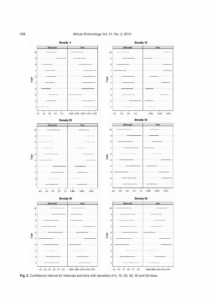
Fig. 2. Confidence interval for intercept and time with densities of 5, 10, 20, 30, 40 and 50 bees.

and in using longitudinal analysis done by thegeneralized estimating equations (GEE) it was notpossible to identify a correlation structure to explainthe possible temporal dependence mortality causedby A. mellifera confined within the same cages overtime. Therefore, there is evidence to say that themixed model approach through the study of theeffect of density performed better in detecting atemporal correlation structure for studies of thisnature, involving A. mellifera

Depending on the adjusted model (Table 2), theresults shown in Fig. 2 correspond to the confi-dence intervals for the individual profiles (cages),each adjusted by density. Thus, it is noted that forlow densities 5, 10 and 20 bees (Fig. 2) there isevidence that the random effect of time is mostpronounced in relation to the effect of the inter-cept in estimating the mean mortality for the beesstudied in each cage. However, when increasingthe density to 30, 40 and 50 individuals (Fig. 2) therandom time effect was almost similar to the inter-cept effect. This fact was apparent for all cages,specifically at higher densities.

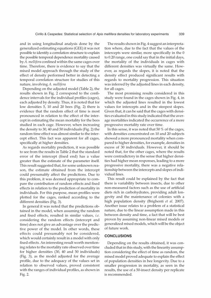
As regards mortality prediction, it was possibleto see from the results in Table 2 that the standarderror of the intercept (fixed end) has a valuegreater than the estimate of the parameter itself.This result suggested that, for some unknown rea-son, the estimate obtained from the interceptcould presumably affect the predictions. Due tothis problem, it was deemed appropriate to com-pare the contribution of random effects and fixedeffects in relation to the prediction of mortality inindividuals. For this purpose, mean profiles wereplotted for the cages, ranked according to thedifferent densities (Fig. 3).

In general it was noted that the predictions ob-tained in the model, when assuming the randomand fixed effects, resulted in similar values, i.e.considering the random effects (intercept andtime) does not give an advantage over the predic-tive power of the model. In other words, theseeffects could presumably not be considered,which would certainly result in a model with onlyfixed effects. An interesting result worth mention-ing relates to the mortality rate observed over timefor higher densities (30, 40 and 50 individuals)(Fig. 3), as the model adjusted for the averageprofile, due to the adequacy of the values set inrelation to observed values, proved consistentwith the ranges of individual profiles, as shown inFig. 2.

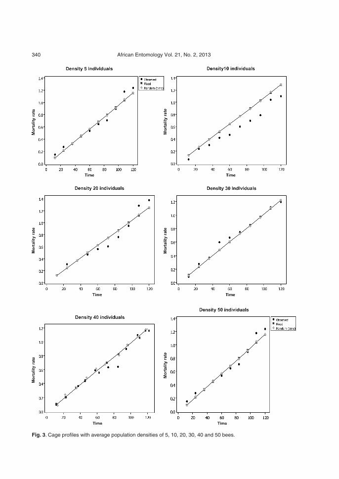
The results shown in Fig. 4 suggest an interpreta-tion where, due to the fact that the values of theintercepts were similar, more specifically in the 0to 0.20 range, one could say that in the initial days,the mortality of the individuals in cages withdifferent densities was virtually the same. How-ever, as regards the slopes, it is noted that thedensity effect produced significant results withregards to mortality progression. This situationwas inferred by the adjusted lines in each density,for all cages.

The most promising results considered in thisstudy were found in the cages shown in Fig. 4, inwhich the adjusted lines resulted in the lowestvalues for intercepts and in the steepest slopes.Given that, it can be said that the cages with densi-ties evaluated in this study indicated that the aver-age mortalities indicated the occurrence of a moreprogressive mortality rate over time.

In this sense, it was noted that 50 % of the cages,with densities concentrated on 10 and 20 subjectsshowed a more pronounced mortality when com-pared to higher densities, for example, densities inexcess of 30 individuals. However, it should benoted that, for the other cages, where the resultswere contradictory in the sense that higher densi-ties had higher mean responses, leading to a moreprogressive mortality, there was a negative rela-tionship between the intercepts and slopes of indi-vidual lines.

This result could be explained by the fact thatthere is variability between insects, due to othernon-measured factors such as the use of artificialdiets rich in carbohydrates, providing adult lon-gevity and the maintenance of colonies with ahigh population density (Brighenti et al. 2007).Another issue relates to a problem of a statisticalnature, due to the linear assumption made in thisbetween density and time, a fact that will be bestproven by assuming non-linear mixed models orgeneralized mixed models, which will be the objectof future work.

CONCLUSIONS

Depending on the results obtained, it was con-cluded that in this study, with the linearity assump-tion considering the effect of time as random, themixed model proved adequate to explain the effectof population densities in bee longevity. Due to asmaller progression in mortality, as seen in theresults, the use of a 50-insect density per replicateis recommended.

Cirillo & Cespedes: Statistical selection of Apis mellifera densities for laboratory experiments 339

340 African Entomology Vol. 21, No. 2, 2013

Fig. 3. Cage profiles with average population densities of 5, 10, 20, 30, 40 and 50 bees.

REFERENCES

ALAUX, C., BRUNET, J., DUSSAUBAT, C., MONDET, F.,TCHAMITCHAN, S., COUSIN, M., BRILLARD, J.,BALDY, A., BELZUNCES, L.P. & CONTE, Y.L. 2010.Interactions between Nosema microspores and aneonicotinoid weaken honeybees (Apis mellifera).Environmental Microbiology 12(3): 774–782.

BIESMEIJER, J.C., ROBERTS, S.P., REEMER, M.,OHLEMULLER, R., EDWARDS, M., PEETERS, T.,SCHAFFERS, Z.P., POTTS, S.G., KLEUKERS, R.,THOMAS, C.D., SETTELE, J. & KUNIN, W.E. 2006.Parallel declines in pollinators and insect-pollinatedplants in Britain and the Netherlands. Science 313:351–354.

BRIGHENTI, D.M., CARVALHO, C.F., CARVALHO,G.A., BRIGHENTI, C.R.G. & CARVALHO, S.M. 2007.Bioatividade do Bacillus thuringiensis var. kurstaki(Berliner, 1915) para adultos de Apis mellíferaLinnaeus, 1758 (Hymenoptera: Apidae). Ciência eAgrotecnologia [online], 31(2): 279–289.

BRIGHENTI, C.R.G., CIRILLO, M.A. & BRIGHENTI,D.M. 2008. Análise longitudinal na determinaçãodo foto período adequado para criação de abelhasem laboratório. Biometric Brazilian Journal 26(3):111–124.

BRIGHENTI, D.M., BRIGHENTI, C.R.G., CIRILLO, M.A.& SANTOS, C.M.B. 2010. Optimization of the compo-

Cirillo & Cespedes: Statistical selection of Apis mellifera densities for laboratory experiments 341

Fig. 4. Individual profile for cages 3, 5, 6, 8 and 10 at different densities.

nents of an energetic diet for Africanized beesthrough the modelling of mixtures. Journal ofApicultural Research 49(4): 326–333.

BURGES, H.D. 1978. Control of wax moths: physical,chemical and biological methods. Bee World 59(4):129–138.

CARVALHO, M.D.F. 2009. Temperatura da superfíciecorpórea e perda de calor por conveção emabelhas(Apis mellifera) em uma região semiárida. Dissertaçãode Mestrado, Universidade Federal Rural do Semi-Árido, Mossoró, Rio Grande do Norte, Brazil.

CHENG J., EDWARDS, L.J., MALDONADO-MOLINA,M.M., KOMROC, K.A. & MULLERA, K.E. 2010. Reallongitudinal data analysis for real people: building agood enough mixed model. Statistics in Medicine 29:504–520.

DIGGLE, P.J., HEAGERTY, P., LIANG, K.Y. & ZEGER,S.L. 2002. Analysis of Longitudinal Data. 2nd Edn.Clarendon Press, Oxford, U.K.

GALLAI, N., SALLES, J.M., SETTELE, J. & VAISSIERES,B.E. 2009. Economic valuation of the vulnerability ofworld agriculture confronted with pollinator decline.Ecological Economics 68: 810–821.

HARRISON, J.M. 1987. Roles of individual honeybeeworkers and drones in colonial thermogenesis.Journal of Experimental Biology 129: 53–61.

HEINRICH, B. 1979. Thermoregulation of African and

European honeybees during foraging attack andhive exits and returns. Journal of Experimental Biology80: 217–229.

KRONENBERG, F. & HELLER, C. 1982.Colonialthermoregulation in honey bee (Apis mellifera). Jour-nal of Comparative Physiology 148: 65–76.

LITTELL, R.C., HENRY, P.R. & AMMERMAN, C.B. 1998.Statistical analysis of repeated measures data usingSAS procedures. Journal of Animal Science 76: 1216–1231.

R DEVELOPMENT CORE TEAM. 2010. R: A Languageand Environment for Statistical Computing. R Founda-tion for Statistical Computing, Vienna, Austria. On-line at: http://www.R-project.org

RICKETTS, T.H., REGETZ, J., STEFFAN-DEWENTER, I.,CUNNINGHAM, S.A., KREMEN, C., BOGDANSKI,A., GEMMILL-HERREN, B., GREENLEAF, S.S.,KLEIN, A.M., MAYFIELD, M.M., MORANDIN, L.A.,OCHIENG, A., POTTS, S.G. & VIANA, B.F. 2008.Landscape effects on crop pollination services: arethere general patterns? Ecology Letters 11(5): 499–515.

RINDERER, T.E. & BAXTER, J.R. 1978. Honey bees:the effect of group size on longevity and hoarding inlaboratory cages. Annals of the Entomological Society ofAmerica 71(5): 732–732.

VERBEKE, G. & MOLENBERGHS, G.2009. Linear MixedModels for Longitudinal Data. 2nd Edn. Springer Seriesin Statistics and Computing, New York, U.S.A.

Accepted 4 May 2013

342 African Entomology Vol. 21, No. 2, 2013