SSCL-Preprint-52

Superconducting Super Colli<ier Laboratory

.: .... .......

........ .... .

.....

......

:.. .... :: ........ : ... .

. ............ ,,' . •.....

.;:' .:)(;: .... ::;:::::: ........ . "': ,:' ..... "',' < ..

" ...... :... . .. / ..... " ..... : .. ,.'

~ ... ~ .. .....

/ ..:'

.... , . ..:" .......•••..• . .. :':'

A Statistical Rationale for Establishing Process Quality Control Limits Using

Fixed Sample Size, for Critical Current Verification of SSC Superconducting Wire

D. A. Pollock, G. Brown, D. W. Capone II, D. Christopherson, J. M. Seuntjens, and J. Woltz

March 1992

To be published in Supercollider 4

A Statistical Rationale for Establishing Process Quality Control Limits Using

Fixed Sample Size, for Critical Current Verification of sse Superconducting Wire·

D. A. Pollock, G. Brown, D. W. Capone n, D. Christopherson, J. M. Seuntjens, and J. Woltz

Superconducting Super Collider Laboratoryt 2550 Beckleymeade Ave.

Dallas, TX 75237

March 1992

SSCL-Preprint-52

·Presented at the International Industrial Symposium on the Super Collider, New Orleans, March 4-6,1992.

tOperated by the Universities Research Association, Inc., for the U.S. Department of Energy under Contract No. DE-AC35-89ER40486.

A STATISTICAL RATIONALE FOR ESTABLISHING PROCESS QUALITY CONTROL LIMITS USING FIXED SAMPLE SIZE, FOR CRITICAL CURRENT VERIFICATION OF SSC SUPERCONDUCTING WIRE

D. A. Pollock, G. Brown, D. W. Capone II, D. Christopherson, J.~.Seungens,J. Woltt

Superconducting Super Collider Laboratory * 2550 Beckleymeade Avenue Dallas, Texas 75237

INTRODUCTION

Quality verification of a design characteristic of a manufactured product is typically achieved through inspection or sampling. In the case of superconducting wire critical current, the product of one billet is presently required to be verified by testing one sample from each piece of wire generated by the supplier's process. In some cases. the number of tests per billet is very large. (i.e.>40). It is expected that once the Phase I part of the Vendor Qualification Program is complete. fewer samples per billet will be necessary. both by choice and because of anticipated improvements in manufacturing methods. As a tool for monitoring process uniformity. current SS~ plans call for applying statisticallUnits to each supplier's process. after a sufficient number of billets have been produced to establish process expectations. This paper addresses two questions regarding the issue of sampling frequency and process control. First, how many wire piece measurements from one billet (or production unit 1) are sufficient for verifying billet performance to specification? Second. how far can the measured average and range for a billet be from the established process center and standard deviation before it is considered non-representative of the stable process expectations?

The purpose of this paper is to demonstrate a statistical method for verifying superconducting wire process stability as represented by Ie. The paper does not propose changing the Ie testing frequency for wire during Phase I of the present Vendor Qualification Program. The actual statistical limits demonstrated for one supplier's data are not expected to be suitable for all suppliers. However. the method used to develop the limits and the potential for improved process through their use. may be applied equally.

Implementing the demonstrated method implies that the current practice of testing all pieces of wire from each billet, for the purpose of detecting manufacturing process errors (i.e. missing a heat-treatment cycle for a part of the billet, etc.) can be replaced by other less costly process control measures. As used in this paper process control limits for critical current are quantitative indicators of the source manufacturing process unifonnity. The limits serve as alanns indicating the need for manufacturing process investigation.

* Operated by the Universities Research Association. Inc., for the U.S. Department of Energy under Contract No. DE-AC35-89ER40486.

1

Upstream sequences in the process are not pan of this discussion, however they are equally in need of direct on-line control, to the extent that they can be shown to influence product performance.

SAMPLING THEORY AND STATISTICAL SIGNIFICANCE

Two parameters are typically used to describe the center and the magnitude of variability in the distribution of a continuous variable, the mean UL. simple average) and the standard deviation (a, a measure of distribution dispersion).2 When the observations of interest confonn to a known probability distribution (i.e. Nonnal, Exponential, etc.), a significant amount of information may be inferred from J.1 and a. Given an approximately normal distribution, the likelihood (probability) that a given observation from the distribution will fall within a panicular range of the mean may be predicted, as a function of J.1 and a, and is typically stated as a proportion of the area under the nonnal curve with a range of 0 to 1. 3

In their fonnal sense, J.1 and a are based on full or complete information from the source population. When a collection of observations consists of a partial accounting, the collection is a sample. The corresponding sample distribution parameters, mean and standard deviation are identified XBAR (J.1X> and S (ax). 4 Any number of Ie measurements from one billet is a sample. Practical sample size is limited to the number of pieces generated from each billet. Economic sample size is based on: 1.) the cost of sampling; 2.) the properties of the process distribution; and 3.) the level of security and sensitivity to change that is necessary.

The Shewhart XBAR RControl Chart

Statistical Quality Control (SQC) methods have been developed to test the performance of samples against their expected population parameters. The methods diseused in this paper were developed by Walter Shewhart in the 1920's, from procedures for confidence interval estil1UUion and statistical hypothesis testing. S In the generalized method, one compares a sample parameter (typically average and range, or standard deviation) for a given number of observations (a subgroup) to the expected population value. If the population parameters are unknown, they must first be estimated by means of an evaluation of recent data from a stable process. Given the sample is a true representative of the population, the parameter may be expected to fall within a certain distance of the population center line. The allowable distance from the center is based on the level of control desired, the subgroup size and the value of the population mean and standard deviation. If the sample parameter falls outside the defined control limits, the method indicates that the product represented by the sample is lilcely from an alternate population, (i.e. a statistically significant assignable cause change has occUl'l'Cd). 6

One of the basic statistical tools for monitoring a process, called the XBAR R chart, will be demonstrated. The application of this method involves taking samples from a process at fixed intervals. The sample is made up of a fixed number of measurements called a subgroup. The subgroup average (J.1x) and the range (R) are calculated and compared to the established control limits for the sample average and the Range. For the critical current case, the logical sampling interval is each billet (or production unit) and the subgroup is the number of measurements performed to verify the product. Assuming the manufacturer produces billets as single production units, the subgroup average is a measure of between billet variation, and R is a measure of within billet variation.

2

Factors in Determining Acceptable Control Limits

The XBAR R procedure defines limits for the variability of sample averages and ranges based on the level of natural variation in the process and choices made when designing the chart. The key choices are the level of risk one is willing to tolerate (designated Cl and 13 probabilities), and the subgroup size (n) selected for each sample. The probability that a given sample average will be inside the selected control limits is defined by 1 - Cl. As Cl is increased for a fixed n, the control limits move closer to the center line, and the tolerance for allowed process drift is reduced, but the probability that a sample average will be within the limits is also reduced. (i.e. more false alarms may be expected to occur). 13 is a measure of the sensitivity of the control limits to systematic process drift, it is the probability that a sample mean will be within the control limits when in fact it is really a representative of an alternate process mean and should be rejected by the model. As n is increased for a fixed Cl,

the control limits for sample average are narrowed while the 13 probability is reduced. Larger subgroup size improves the overall performance of the XBAR R model, but with the negative effect of increased sampling cost. Balancing sampling risk against cost is the challenge for those implementing process controls.

THE REFERENCE DATA SET

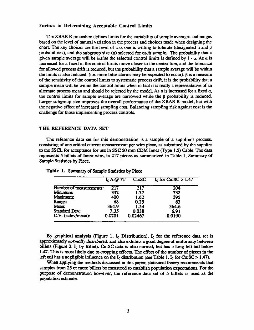
The reference data set for this demonstration is a sample of a supplier's process, consisting of one critical current measurement per wire piece, as submitted by the supplier to the SSCL for acceptance for use in sse 50 mm COM Inner (Type 1.5) Cable. The data represents 5 billets of Inner wire, in 217 pieces as summarized in Table 1, Summary of Sample Statistics by Piece.

Table 1. Summary of Sample Statistics by Piece

Number of tneaSUl'e1l1Cnts: Minimum: Maximmn: Range: Mean: StandaId Dev: C.V. (stdev/mean):

IeA@7T

217 332 400

68 364.9 7.35

0.0201

Cu:se

217 1.37 1.62 0.25 1.54

0.038 0.02467

Ie for Cu:se > 1.47

204 332 395 63

364.6 6.91

0.0190

By graphical analysis (Figure 1. Ie Distribution), Ie for the reference data set is approximately normally distributed, and also exhibits a good degree of uniformity between billets (Figure 2. Ie by Billet). cu:se data is also normal, but has a long left tail below 1.47. This is most likely due to cropping effects. The effect of the number of pieces in the left tail has a negligible influence on the Ie distribution (see Table I, Ie for Cu:se > 1.47).

When applying the methods discussed in this paper, statistical theory recommends that samples from 25 or more billets be measured to establish population expectations. For the purpose of demonstration however, the reference data set of 5 billets is used as the population estimate.

3

=: < = =: ~ /:1.0

Z 0 -1-0 =: 0 /:1.0 0 =: /:1.0

60 0.25

50 0.20 40 0.15 30

0.10 20

0.05 10

330 344 358 372 386 400

Ie FOR ALL PIECES. (A @ 1T. 0=211)

Figure 1. Ie Distribution. A frequency histogram of the source data Ie distribution.

n 0 c: :z: -i

u -

405

385

34S

325

0

•

,~~~ ~ 0

ABC D E

BILLET

Figure 2. Ie by Billet A Box Plot of Ie variation within and between billets.

PRELIMINARY XBAR CONTROL LIMIT CALCULATION

The following example describes the general method for calculating control limits when J.L and a are known. The text references should be consulted for a fuller treatment of the method for calculating limits where J.L and a are estimated from process data. The example calculates ±3alimits for XBAR. 7.8

Process Control limits = [J.L ± (Z a/2 ) • ( a/..Jn)] ; for J.L and a known.

z = [(x - J.L) /a], the "standard normal deviate". Z aI2 = the value of Z to the right or left of J.L which delimits the area under the normal curve at a/2. For 3a control limits Z a/2 = 3. Given that J.L = 364.9 A @ 7T ,a = 7.35 A, n = 30, and a = 0.0027:

J.L Upper Control Limit = 368.93 A @ 7T J.L Lower Control Limit = 360.87 A @ 7T

These limits mean that if the true process mean is J.L and the standard deviation is a, a sample of 30 randomly selected wire measmements from the process is expected to have an average which falls between 360.87 A and 368.9 A, 99.73 times out of 100.

The Effect of a and n on the Control Limits

As mentioned earlier, a risk and subgroup size (n) have an effect on the width of the calculated control limits. A demonstration of their effect is presented in Figures 3 and 4. Figure 3, Subgroup Size Effect, plots XBAR upper control limits as a function of n, using the general formula and the expected process J.L and a, for subgroups n = 1,2,3 ... 30. Figure 4. Effect of a on Control Limits shows how control limits change with a risk, for a < 0.40. Both Figure 3 and 4 use J.L = 364.9 and a = 7.35. 1- a is a measure of the probability that a given XBAR will be inside the designated control limits. In figure 4, sigma limits for XBAR are labeled for frequently used a levels. Typically 2CJ (a = 0.0455) or 3a (a = 0.0027) conttollimits are selected for manufacturing process control purposes, since they provide a good level of confidence without expecting a large number of out-of-

4

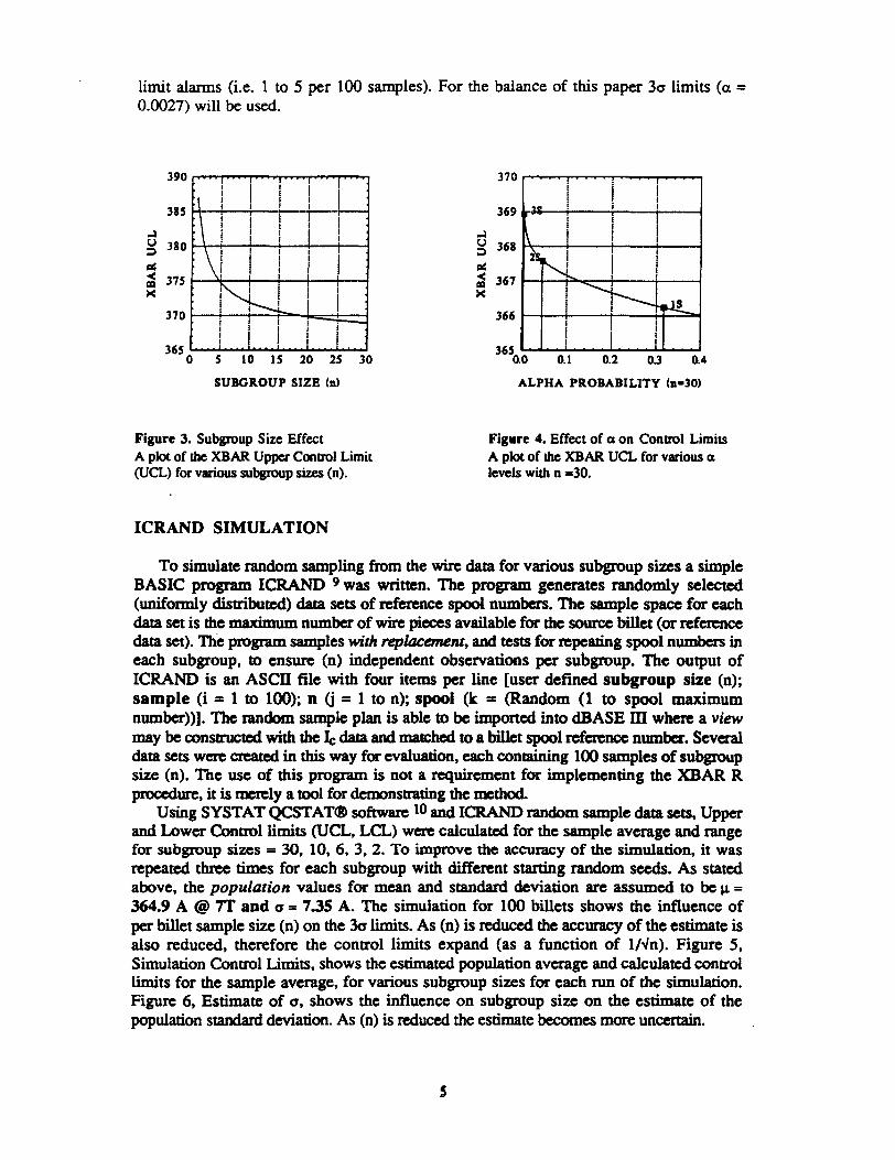
limit alarms (i.e. 1 to 5 per 100 samples). For the balance of this paper 30' limits (a = 0.(027) will be used.

390

385

...:a u 380 ::> II1II -< 375 CD ><

370

365 0 5 10 15 20 25 30

SUBGROUP SIZE (n)

Figure 3. Subgroup Size Effect A plot of die XBAR Upper Conb"Ol Limit (UCL) for various subgroup sizes (D).

ICRAND SIMULATION

...:a u ::> II1II -< CD ><

370

369

368

367

366

365 0.0 0.1 0.2 0.3 0.4

ALPHA PROBABILITY (n-30l

Figure 4. Effect of a 00 Coob"Ol Limits A plot of die XBAR UCL for various a levels with 0 =30.

To simulate random sampling from the wire data for various subgroup sizes a simple BASIC program ICRAND 9 was written. The program generates randomly selected (uniformly disaibuted) data sets of reference spool numbers. The sample space for each data set is the maximum number of wire pieces available for the source billet (or reference data set). The program samples with replacement, and tests for repeating spool numbers in each subgroup, to ensure (n) independent observations per subgroup. The output of ICRAND is an ASCn file with four items per line [user defined subgroup size (n); sample (i = 1 to 100); n (j = 1 to n); spool (k = (Random (1 to spool maximum number»]. The random sample plan is able to be imported into dBASE m where a view may be constructed with the Ie data and matched to a billet spool reference number. Several data sets were created in this way for evaluation, each containing 100 samples of subgroup size (n). The use of this program is not a requirement for implementing the XBAR R procedure, it is merely a tool for demonsttating the method.

Using SYSTAT QCSTAT® software 10 and ICRAND random sample data sets, Upper and Lower Control limits (UCL, LCL) were calculated for the sample average and range for subgroup sizes = 30, 10, 6, 3, 2. To improve the accuracy of the simulation, it was repeated three times for each subgroup with different starting random seeds. As stated above, the population values for mean and standard deviation arc assumed to be J1 = 364.9 A @ 7T and 0' = 7.35 A. The simulation for 100 billets shows the influence of per billet sample size (n) on the 30" limits. As (n) is reduced the accuracy of the estimate is also reduced, therefore the control limits expand (as a function of INn). Figure 5, Simulation Control Limits, shows the estimated population average and calculated control limits for the sample average, for various subgroup sizes for each run of the simulation. Figure 6, Estimate of 0', shows the influence on subgroup size on the estimate of the population standard deviation. As (n) is reduced the estimate becomes more uncertain.

1= 390 ... ® ~ 380

r: :E 370 ::i ~ 0 360 III

'"' Z; 0

350 CJ III < III

340 ~ 0 5 10 15 20 2S

SAMPLE SUBGR.OUP SIZE CD)

Figure S. Simulation Control Limits Simulation results for the estimate of J.l.

c MEAN v LCL AUCL

30

and UCI./LCL for various subgroup sizes (n).*

1= 10 ... ® < 9 C > III Q <It I g,; 0 !s < 7 :E 0 ;; 6 110 C 0

5 5 0 6 12 11 24

SAMPLE SUBGR.OUP SIZE CD)

Figure 6. Estimate of a Simulation results for the estimate of a. for various subgroup sizes (n). *

* Based on 100 random samples of subgroup size n. selected from the reference data seL

SENSITIViTy OF THE LIMITS TO PROCESS DRIFT

30

A rationale for selecting the acceptable subgroup size should include a consideration of the sensitivity of the limits to systematic process change (or drift). If the process mean shifts up or down, what is the probability the change will be detected by the XBAR model? The answer again depends on J1, a, n, a, as well as a concept from hypothesis testing known as the power of the test, denoted 1 - ~. 11 Table 2, Possible Decisions in Hypothesis Testing, describes the choices that may be made when applying statistical significance tests. 12 HO is the null hypothesis (i.e. J1 = 365) and HA is the alterntJte hypothesis (i.e. J1 ~ 365). When a statistical decision is made, it is subject to a and ~ error probabilitie~, also only one state can be a trUe representative of the process. The power concept provides a means of quantifying ~ error probabilities.

Table 2. Possible Decisions in Hypothesis Testing

STATE -. TRUE Situation

DECISION J.

ACCEPT He

REJECT He

(Ho is Correct)

Correct Decision P(Ho)-(l-a)

IncolTect Decision P( a ) ; Type I E"or

TRUE Situation (HA is Correct)

InCOlTCCt Decision P( IS ) ; Type II Error

Correct Decision P(HA> = ( 1 - IS )

The power of the test (1 -~) against HA at the a significance level is the probability that a normal deviate (Z) lies in one of the two regions: Z < Z 1 or Z > Zl. 13

1 - ~ = P(HA> = [P(Z < Zl> + P( Z> ZV] where: Zl= (- .In/a)*{J1A - JJO) - Za and Z2= (- .In/a)*{J1A - JJO) + Za

For He: J1 = 365, n = 30, a = 7.564, a = 0.0027, the probability that He will be rejected (i.e. the sample average will fall outside the 365 ± 3c:r limits) if HA: the actual or True process mean drifts 1.4% to 360 is 0.80. For the reference data set, to have a probability better than 0.80 of detecting a change in the process mean, with a one billet sample of 6

6

measurements, the process mean would have to shift by more than ± 3.3%, (± 12 A). For a sample subgroup size of 3 (as currently defined in the SSC wire specification 14) the process center would have to drift by ± 4.4%, (± 16 A) for I-P = 0.80. An Operating Characteristic curve is useful for visualizing IJ risk. is See Figure 7, OC Curve (n = 30 and n = 6, a = 0.(027), in which p probabilities are shown as a function of alternate means.

1.0

f! 2 0.1 :3 Z ;: 0.6 !: ~

0.0 ................................................................................. ......... 350 355 360 365 370 375 310

TllUE PllOCESS MEAN

Figure 7. OC Curve (n := 30 and n ... 6, a := 0.00(7) The Operating Characteristic: curve plots ~ against possible alternate means, where ~ is the probability that an alternate mean will be accepted by the J.IO control limits.

Testing the Control Limits

To demonstrate the sensitivity of the limits to a change in JJ. a sample data set was made by adding 3% to the Ie's from a source billet The artificial billet data was then tested against the population estimate. As may be expected, for a process with the UCL 2.5% above the process center, the majority of the observations from the artificial data set were above the upper limit, (see Figure 8. Effect of +3% Process Shift). From the OC Curve for the process with an alternate mean of 376 and n = 6, it is expected that 25.5% of the J1x'S will be within the J.IO = 365 limits. The simulation had 4 (16%) sample averages with the limits. So. using only 2S samples of subgroup size 6. the simulation confirms the model expectations. Had this data been from a real billet (with only 6 short sample measurements randomly selected from the finished wire). there is a relatively strong probability ( 1- P ~ 0.745) that the process shift of 3% would have been detected.

390

380 i-o .... @)

< 370

u -360

350 0

. . .: ..

. .

5 10

: .

. . .. •

15

SAMPLE (nz 6)

. . • ••

20

Figure 8. Effect of + 3% Process Shift

7

ua. -"4

LCL - lSi

2S

Figure 8 shows both the individual observations (filled box) and the J.1x's (open box with connecting line), to demonstrate the sensitivity of the XBAR model to a 3% shift in the mean. In practice the individuals would not be plotted. Note that all of the J.1x's are at or above the upper conttollimit, indicating a significant change has occurred.

CONCLUSION

This work has demonstrated the statistical concepts behind the XBAR R method for detennining sample limits to verify billet Ie performance and process unifonnity. Using a preliminary population estimate for J1 and a from a stable production lot of only S billets, we have shown that reasonable sensitivity to systematic process drift and random within billet variation may be achieved, by using per billet subgroup sizes of moderate proportions. The effects of subgroup size (n) and sampling risk (a and p) on the calculated conttollimits have been shown to be important factors that need to be carefully considered when selecting an actual number of measurements to be used per billet, for each supplier process. Given the present method of testing in which individual wire samples are ramped to Ie only once, with measurement uncenainty due to repeatability and reproducibility (typically> 1.4%) 16, large subgroups (i.e. >30 per billet) appear to be unnecessary, except as an inspection tool to confirm wire process history for each spool. The introduction of the XBAR R method or a similar Statistical Quality Control procedure is recommend for use in the superconducting wire production program, particularly when the program transitions from requiring tests for all pieces of wire to sampling each production unit.

REFERENCES

1. SS(1 document, M35-000014: NbTi Superconducting Wire For SSC Dipole Magnets (1.3 Grade Inner), paragraph 3.3.1 and 4.4.2.

2. D. C. Montgomery, "Introduction To Statistical Quality Control", John Wiley & Sons, New Yorlc, 1991, pp. 34 ff.

3. E. L. Grant and R. S. Leavenworth, "Statistical Quality Control", McGraw-Hill, New York, 1988, pp. SO ff.

4. ibid Montgomery, p. 60. S. ibid Montgomery, p. 105. 6. ibid Montgomery, p. 103. 7. ibid Montgomery, pp. 203 ff. 8. ibid. Grant, pp. 78 ff. 9. D. Pollock and G. Brown, ICRAND.BAS program. 10. H. Stenson, "QCSTAT version 1.1: A Supplementary Module for SYSTAT",

SYSTAT, Inc., Evanston, n... 1990, pp. 37 ff. 11. M. Ben-Horim and H. Levy, "Statistics: Decisions And Applications In Business

And Economics", Random House. New York, 1984, p. 444. 12. ibid. p. 424. 13. G. W. Snedecor and W. G. Cochran, "Statistical Methods", Iowa State University

Press, Ames, Iowa, 1980, p. 69. 14. ibid. SS(1 document, M3S-()()()()14, paragraph 4.4.2. IS. J. M. Juran and F. M. Gryna. "Juran's Quality Control Handbook", McGraw-Hill,

New York, 1988, pp. 24.10 ff. 16. M.J. Erdmann, D. A. Pollock, and D.W. Capone II, "Quantification of Systematic

Error in Ie Testing", Supercollider 3, Plenum Press, New York, 1991, pp. 713 ff.

8