1

This is an Author’s Accepted Manuscript of an article published in

The Journal of Quantitative Linguistics, 2010, Vol. 17, p191-211.

(Copyright: Taylor and Francis)

Available on line at

http://www.tandfonline.com/10.1080/09296174.2010.485445

A STATISTICAL STUDY OF FAILURES

IN SOLVING CROSSWORD PUZZLES

S. Naranan

20 A/3, Second Cross Street,

Jayaramnagar, Thiruvanmiyur,

CHENNAI 600-041,

India.

e-mail: snaranan@gmail.com

10 January 2010

Revised: 16 July 2010.

2

ABSTRACT

Crossword puzzles are the most popular form of linguistic puzzles; for the

solver they are intellectually challenging and entertaining as well. An interesting

exercise for this author, a keen solver of the British style ‘cryptic’ crossword puzzles,

has been the statistical distribution of the number of unsolved clues (x) in a puzzle.

Data are cumulated over a decade (total number of puzzles 3404). The large sample

size makes it possible to examine the tail of the distribution at large x, up to 12. It is

found that the Poisson Distribution with one free parameter (λ) is inadequate, but the

Negative Binomial Distribution (NBD) with two free parameters (p,k) fits the

distribution well as vouched by a χ2-test. The NBD can be interpreted as a “mixture”

of Poisson and Gamma Distributions . It is suggested that this is an appropriate model

for the distribution of x.

Surprisingly, a 3-parameter Lognormal Distribution (LND2) also fits the

observed distribution of x equally well. The popular model for LND – ‘theory of

proportional effect’ – does have some relevance for the crossword puzzle solving. It

appears that the dichotomy (NBD and LND2) exists only for a limited range of (p,k)

of the NBD. Both the NBD and LND2 have wide application in many branches of

science. It is conjectured that NBD may apply to all crossword puzzles and all

solvers. The present work has relevance to linguistics, especially the co-existence of

random and orderly features as reflected in the many statistical regularities of

language texts.

3

1. INTRODUCTION

Crossword puzzles are the most popular word puzzles and are daily features in

almost all the widely read newspapers and magazines in the world. Typically a

puzzle consists of a square grid (say 15 x 15) with words, ‘across’ and ‘down’

(crosswords) delineated by a symmetrically-placed set of black squares. The number

of words is about 30 (28 to 34 in most 15 x 15 grids) roughly shared equally by

‘across’ and ‘down’ and each crossword is the solution of a ‘clue’ accompanying the

grid. Occasionally a clue can include more than one crossword. The placement of the

black squares is subject to the condition that the grid pattern remains the same when

rotated by 1800. To begin with, the grid is blank and the solver has to fill in the words

with the help of the clues.

Crossword puzzles can be broadly classified into two types: (1) the American

style and (2) the British style (cryptic). There is considerable difference between the

two in the grid structure, types of words and the style of the clues. In Britain, Europe

and India the cryptic puzzles are very popular. The puzzle described in the previous

paragraph is an example of cryptic puzzle.

In this study we consider only the cryptic crossword puzzles. An interesting

statistic worthy of investigation by a solver is the probability distribution of the

number of unsolved clues in the grid or the number of incomplete words (“failures”).

The distribution clearly depends on many factors including the skills of the composer

and the solver and the clueing style. But these are not generally relevant for the

purely statistical study. We will discuss this aspect later.

2. CROSSWORD PUZZLES: DATA ON FAILURES IN SOLUTION.

I have been an enthusiastic solver of crossword puzzles for over 40 years. In

my active professional life in Mumbai, the puzzles were from the daily ‘Times of

India’ and later after my retirement in Chennai, from the daily ‘The Hindu’. When

the idea of a statistical study of failures arose about 25 years ago, I started to

standardize my style and strategy of solving and recorded the number of unsolved

4

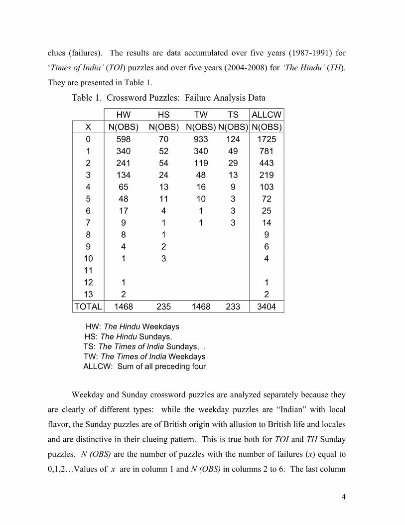
clues (failures). The results are data accumulated over five years (1987-1991) for

‘Times of India’ (TOI) puzzles and over five years (2004-2008) for ‘The Hindu’ (TH).

They are presented in Table 1.

Table 1. Crossword Puzzles: Failure Analysis Data

HW HS TW TS ALLCW X N(OBS) N(OBS) N(OBS) N(OBS) N(OBS) 0 598 70 933 124 1725 1 340 52 340 49 781 2 241 54 119 29 443 3 134 24 48 13 219 4 65 13 16 9 103 5 48 11 10 3 72 6 17 4 1 3 25 7 9 1 1 3 14 8 8 1 9 9 4 2 6 10 1 3 4 11 12 1 1 13 2 2

TOTAL 1468 235 1468 233 3404

HW: The Hindu Weekdays HS: The Hindu Sundays, TS: The Times of India Sundays, . TW: The Times of India Weekdays ALLCW: Sum of all preceding four

Weekday and Sunday crossword puzzles are analyzed separately because they

are clearly of different types: while the weekday puzzles are “Indian” with local

flavor, the Sunday puzzles are of British origin with allusion to British life and locales

and are distinctive in their clueing pattern. This is true both for TOI and TH Sunday

puzzles. N (OBS) are the number of puzzles with the number of failures (x) equal to

0,1,2…Values of x are in column 1 and N (OBS) in columns 2 to 6. The last column

5

is for the totality of puzzles (sum of columns 2 to 5). We note at a first glance: (1) the

number of failures can be as high as 10 – the distribution in x has long tails. For

example for ALLCW, out of a total of 3404 puzzles only 1725 (about 50 %) account

for no failures (x = 0) and about 1 % account for x ≥ 7. (2) There is considerable

variation in the distribution of x in the four categories HW, HS, TW and TS.

3. NEGATIVE BINOMIAL DISTRIBUTION FOR THE PROBABILITY OF

FAILURES.

We can consider the observations as an example of random count data of

integer values (x = 0,1,2….). The first choice to fit such a distribution is usually the

Poisson Distribution (PD), which depends only on one parameter λ.

PD: Prob (x) = e-λ λx / x! (λ > 0, x = 0,1,2…) (1)

(Verify that the sum of Prob (x) over all possible integer values of x is 1). Given a

numerical value for λ the PD can be obtained for all x. The two most fundamental

measures of any frequency distribution are the mean (m = <x>) the weighted average

of x and the standard deviation s (=√ (<x2> - <x>2)). For PD it is easily seen that

m = s2 and further both equal λ. So the Poisson parameter λ is actually the mean m

of the distribution. (See for example Feller 1972)

When variance s2 exceeds m the data is ‘over dispersed’ with a long tail and

an additional parameter, besides λ is required to characterize the distribution. The

Negative Binomial Distribution (NBD) is often invoked for such data (Feller 1972).

The probability distribution or the density function is given by

NBD: P(x) = Prob (x) ={Γ(k+x)/[ Γ(k) x!]} pk qx (k > 0, x = 0,1,2…) (2)

where p and k are the two parameters and q = 1 – p. Here Γ(k) is the Gamma

function defined by

Γ(k) = (k – 1) Γ(k – 1) for k > 1

When k is an integer Γ(k) = k(k-1)(k-2) ….1 = k!. Γ(1) = 1.

6

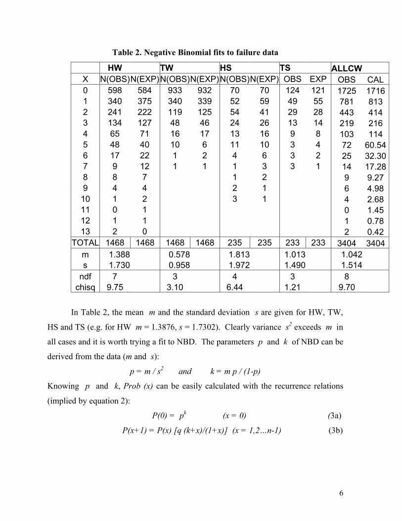
Table 2. Negative Binomial fits to failure data

HW TW HS TS ALLCW X N(OBS) N(EXP) N(OBS) N(EXP) N(OBS) N(EXP) OBS EXP OBS CAL 0 598 584 933 932 70 70 124 121 1725 1716 1 340 375 340 339 52 59 49 55 781 813 2 241 222 119 125 54 41 29 28 443 414 3 134 127 48 46 24 26 13 14 219 216 4 65 71 16 17 13 16 9 8 103 114 5 48 40 10 6 11 10 3 4 72 60.54 6 17 22 1 2 4 6 3 2 25 32.30 7 9 12 1 1 1 3 3 1 14 17.28 8 8 7 1 2 9 9.27 9 4 4 2 1 6 4.98 10 1 2 3 1 4 2.68 11 0 1 0 1.45 12 1 1 1 0.78 13 2 0 2 0.42

TOTAL 1468 1468 1468 1468 235 235 233 233 3404 3404 m 1.388 0.578 1.813 1.013 1.042 s 1.730 0.958 1.972 1.490 1.514

ndf 7 3 4 3 8 chisq 9.75 3.10 6.44 1.21 9.70

In Table 2, the mean m and the standard deviation s are given for HW, TW,

HS and TS (e.g. for HW m = 1.3876, s = 1.7302). Clearly variance s2 exceeds m in

all cases and it is worth trying a fit to NBD. The parameters p and k of NBD can be

derived from the data (m and s):

p = m / s2 and k = m p / (1-p)

Knowing p and k, Prob (x) can be easily calculated with the recurrence relations

(implied by equation 2):

P(0) = pk (x = 0) (3a)

P(x+1) = P(x) [q (k+x)/(1+x)] (x = 1,2…n-1) (3b)

7

These probabilities are multiplied by NT (total number of puzzles in the category

given in the last row of Table 1) and given in Table 2 as N (EXP) (columns

3,5,7,9,11). It is a pure coincidence that NT is the same for HW and TW (1468) .

Even a casual comparison of N (OBS) (repeated from Table 1) and N (EXP)

suggests very good agreement between the two since in most cases the absolute

difference |N (EXP) – N (OBS)| < √N (EXP), the sampling error. However, a more

objective test for ‘goodness of fit of a hypothesis’ – in this case the NBD – to

observed data is the ‘χ2-test’(chi squared test). The χ2 is given in a quasi-symbolic

form as (O-E)2/E summed over all the observed (O) and expected (E) values of N for

x = 0,1,2… The χ2 values and the number of degrees of freedom ndf are given in

Table 2. Here ndf = n-1-l where n is the number of pairs (O, E) and l is the number

of parameters derived from the data (Cramer 1955). Here l = 2 and ndf = n – 3. For

example for HW, χ2 = 9.75 and ndf = 7. From the χ2 tables (Cramer 1955) one finds

that for ndf = 7, χ2 will exceed 12.00 with a probability 0.1 (a value generally adopted

for testing goodness of fit). Similarly for ndf =8, 4, 3, χ2 will exceed 13.4, 7.8 and

6.25 respectively with probability 0.1. Therefore the observed χ2 values (9.75, 3.10,

6.44, 1.21 and 9.70) in Table 2 are all acceptable. In other words the hypothesis of

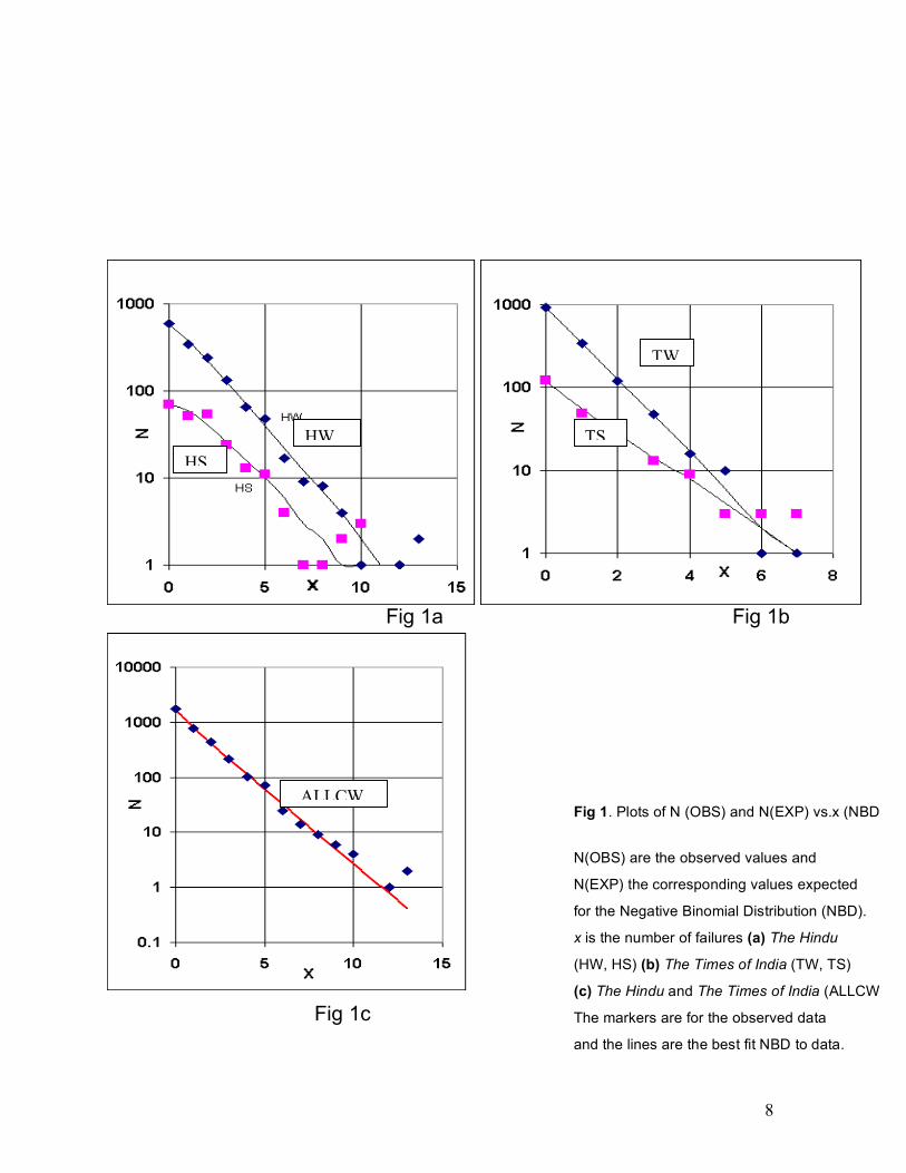
NBD cannot be rejected. In Figure 1 are given the N (OBS) and N (EXP) vs. x for

all the five sets of data.

4. WHY IS THE NBD A CLOSE FIT TO CROSSWORD PUZZLE FAILURE

DATA ?

To understand the effectiveness of NBD for the distribution of the number of

failures in crossword puzzles, we have to first understand the genesis of the Poisson

Distribution based on the concept of Bernoulli trials. Consider repeated independent

trials (or experiments) with only two possible outcomes: failure with probability u

and success with probability v (=1-u). Such trials are called Bernoulli trials. In a

string of n trials the probability of x failures and n-x successes is given by the

Binomial Distribution (BD):

8

Fig 1a Fig 1b

FIG 1b

FIG 1a

Fig 1. Plots of N (OBS) and N(EXP) vs.x (NBD).

N(OBS) are the observed values and

N(EXP) the corresponding values expected

for the Negative Binomial Distribution (NBD).

x is the number of failures (a) The Hindu

(HW, HS) (b) The Times of India (TW, TS)

(c) The Hindu and The Times of India (ALLCW) Fig 1c The markers are for the observed data

and the lines are the best fit NBD to data.

TWWWWW

TS

ALLCW

HW HS

9

BD: Prob(x,n) = ( n x) ux vn-x (x = 0,1,2…) (4)

The name Binomial Distribution (BD) arises from the fact that the above is the xth

term in the binomial expansion (u+v)n. We note incidentally that when summed over

all x we get (u+v)n = 1, since v = 1-u.

When the number of trials n is large and u is low so that nu=λ is a small

number, then the BD becomes the PD (Cramer 1955) as in equation (1)

PD: Prob (x) = e-λ λx / x! (λ > 0, x = 0,1,2….)

It is a remarkable fact that PD has universal application: e.g. radioactive

disintegration, bomb hits of London during the war, wrong connections in telephone

exchange, bacteria cluster counts in blood samples etc, (Feller 1972). Note that PD is

a discrete distribution, only for integral values of x. The key requirements for PD are

low constant probability of failure (u), large sample size (n) and the independent

nature of the trials.

It is clear that PD is inadequate for our data (Section 3 para 3) because the

number of crosswords in a puzzle is small and more importantly the probability of

failure u is not the same for all puzzles because of their in-built diversity, e.g.

different composers, styles of cluing, deliberate introduction of variation in the

complexity of a puzzle. Such variability is reflected in the real world of crossword

puzzles and the observed data will include a mixture of numerous PD’s with different

characteristic parameters (say λ1,λ2,λ3,λ4……). One can model this fact by postulating

that λ is distributed with a probability density function g(λ) with λ > 0. Note λ is a

real number, not just an integer. Then the probability of failures for a given x will be

the sum of probabilities contributed by PD’s with different λ’s weighted by their

density g(λ). So we have Prob(x), which is a ‘mixture distribution’ (MD):

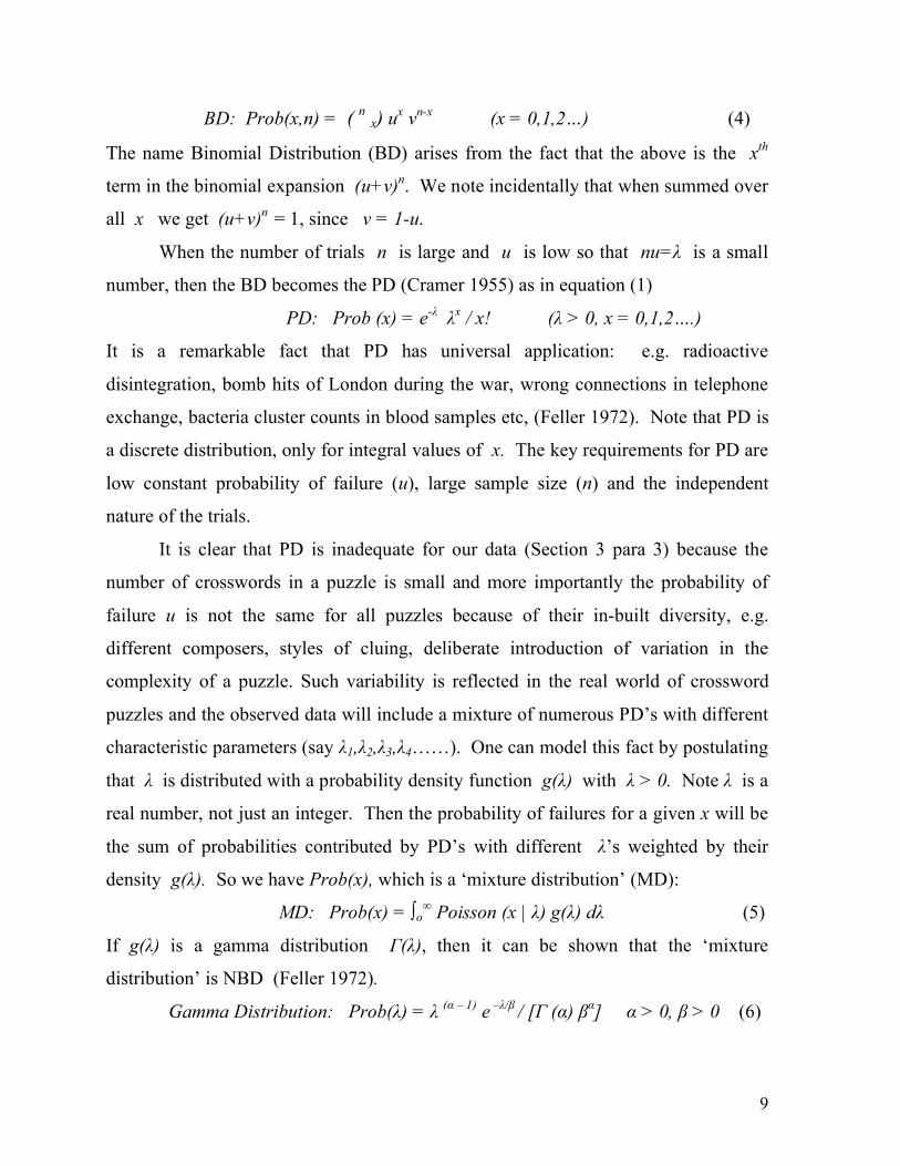
MD: Prob(x) = ∫o∞ Poisson (x | λ) g(λ) dλ (5)

If g(λ) is a gamma distribution Γ(λ), then it can be shown that the ‘mixture

distribution’ is NBD (Feller 1972).

Gamma Distribution: Prob(λ) = λ (α – 1) e –λ/β / [Γ (α) βα] α > 0, β > 0 (6)

10

It has two parameters: α the shape parameter and β the scale parameter. The choice

of a Γ-distribution for g(λ) is very appropriate because it is very similar to the PD; in

fact one may regard the Γ-distribution as - in some sense - a generalization of PD for

a continuous variable (λ). Compare equations (1) and (6); by setting β=1 and noting

that Γ- function is the factorial function. Equation (5) becomes

MD: Prob(x) = {Γ(α+x) / [Γ(α) x!]} (1+β)-α {1-(1/(β+1)}x (7)

By averaging over λ, λ drops out of equation (7) and the NBD depends only on α,β

of the Γ-distribution.

Comparing equations (7) and (2) we note that α,β are related to p,k as

follows.

α = k and β = (1-p)/p

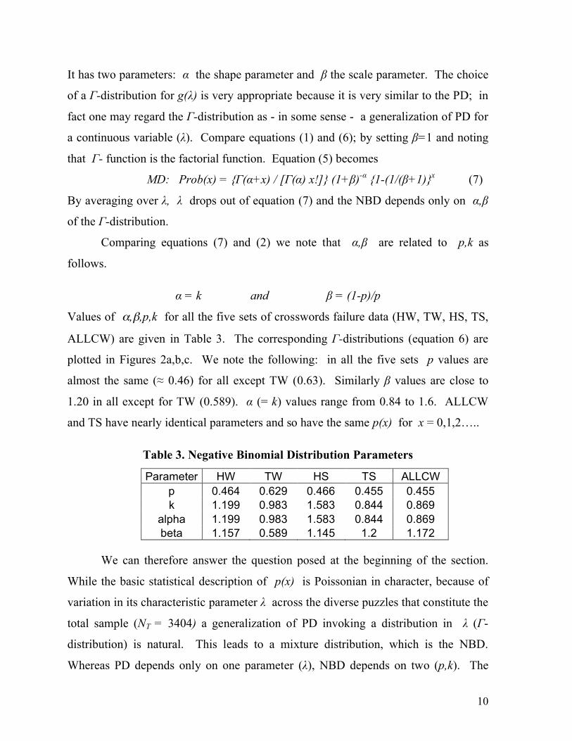
Values of α,β,p,k for all the five sets of crosswords failure data (HW, TW, HS, TS,

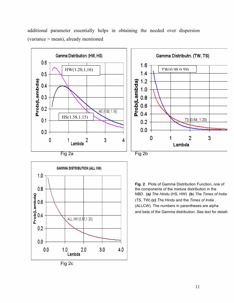
ALLCW) are given in Table 3. The corresponding Γ-distributions (equation 6) are

plotted in Figures 2a,b,c. We note the following: in all the five sets p values are

almost the same (≈ 0.46) for all except TW (0.63). Similarly β values are close to

1.20 in all except for TW (0.589). α (= k) values range from 0.84 to 1.6. ALLCW

and TS have nearly identical parameters and so have the same p(x) for x = 0,1,2…..

Table 3. Negative Binomial Distribution Parameters

Parameter HW TW HS TS ALLCW p 0.464 0.629 0.466 0.455 0.455 k 1.199 0.983 1.583 0.844 0.869

alpha 1.199 0.983 1.583 0.844 0.869 beta 1.157 0.589 1.145 1.2 1.172

We can therefore answer the question posed at the beginning of the section.

While the basic statistical description of p(x) is Poissonian in character, because of

variation in its characteristic parameter λ across the diverse puzzles that constitute the

total sample (NT = 3404) a generalization of PD invoking a distribution in λ (Γ-

distribution) is natural. This leads to a mixture distribution, which is the NBD.

Whereas PD depends only on one parameter (λ), NBD depends on two (p,k). The

11

additional parameter essentially helps in obtaining the needed over dispersion

(variance > mean), already mentioned

Fig 2a Fig 2b Fig 2b Fig 2b Fig. 2. Plots of Gamma Distribution Function, one of the components of the mixture distribution in the NBD. (a) The Hindu (HS, HW) (b) The Times of India (TS, TW) (c) The Hindu and the Times of India . (ALLCW). The numbers in parentheses are alpha and beta of the Gamma distribution. See text for details. Fig 2c

HW(1.20,1,16)

HS(1.58,1.15)

TW(0.98,0.59)

12

(Section 3) whereas in PD, variance = mean. When interpreted as a ‘mixture

distribution’ the NBD is equivalently characterized by α,β (instead of p,k), which

determine the Γ-distribution.

Now we ask: “Is it reasonable to expect NBD to apply for every solver?”

According to the model described, the complexity of crossword puzzles and their

variability will depend both on the solver and the composer(s). There is no reason to

suppose the NBD will not apply universally to all crossword puzzles and solvers. So,

for each solver of crossword puzzles, one can expect NBD to apply, each with a

characteristic pair of parameters (p,k) that quantifies the gap between the skills of the

composer and solver. For the author (p,k) = (0.455, 0.869) (Table 3 ALLCW).

Some readers will be curious about the term “negative” in NBD. It turns out

that equation 2 (NBD) can be rewritten as pk times (-kx) (-q)x

. The latter part is the xth

term in the binomial expansion of (1-q)-k, which has a negative power index.

5. NBD MODELS IN SCIENCE

NBD has diverse applications in behavioral science, e.g. in insurance industry

and marketing of branded products. Car accidents are modeled by NBD, which is

used in determining the insurance premium rates known as “tarification” in insurance

industry (Dionne and Vanasse 1988). In general the number of accidents – low

probability events – among a group of people is not a PD but an NBD (Greenwood

and Yule 1920). In marketing, in a given period the purchases of a branded product

by a random group of consumers follows NBD, which is used to predict purchase

patterns (Ehrenberg 1990). For a comprehensive treatment of NBD and its

applications see the recent “Book of Negative Binomial Regression” by Joseph M.

Hilbe (2007). For a lucid exposition of NBD modeling see Johnson and Vieux

(2006). As an example from physical sciences: in High Energy Particle Physics:

when two energetic elementary particles (like protons from an accelerator) collide, the

13

multiplicity distribution of the newly produced secondary particles in the collision

conforms to NBD (Reference).

There are numerous ways of modeling statistical data or even a particular

distribution like NBD. It is claimed “there are at least a dozen distinct probabilistic

processes that give rise to NBD” (Boswell and Patil 1970). The “mixture

distribution” (Poisson-cum-Gamma distribution) model is only one of them.

Likewise it is possible some probability distribution, other than NBD can also fit the

failure data in crossword puzzles. Note the cautious claim made in section 3 that the

“hypothesis of NBD cannot be rejected” implying that there may exist other

hypotheses which meet the test criteria.

In the next section we pursue this idea further. It is to be emphasized that large

sample sizes help in reducing uncertainties in modeling statistical data. The present

sample size (3404) is modest, but it is 10 years worth of patient work in documenting

the failure data in crossword puzzles. I believe this data is perhaps unique in puzzle

solving behavior although it pertains to an individual (in this case the author).

In early stages of my investigation (about 20 years ago) of crossword puzzle

failure data in a year (small sample size of about 300), it appeared that a lognormal

distribution would fit the data (Aitchison and Brown 1957). As the sample size

increased over the years, it was clear that a simple lognormal distribution (2-

parameter) is not a good fit to the observations. Then it was discovered that NBD

would work! However I never gave up trying lognormal type of distributions since

they have some attractive features in modeling. Actually it turns out that a 3-

parameter lognormal distribution will satisfy the observed data with χ2 values

comparable to those obtained with NBD.

6. THE LOGNORMAL DISTRIBUTION

The normal density function (ND) is given by

ND: Prob(x) = (1/σ√2π ) exp [-(x-m)2/2σ2] -∞ < x < ∞ (8)

14

where m is the mean and σ is the standard deviation. The function is symmetric

about x = m and is “bell-shaped”. An important variant of the ND is the lognormal

distribution (LND); in LND, ln x is normally distributed:

LND1: Prob(x) = (1/σ√2π )(1/x) exp [-( ln x-m)2/2σ2] x >0 (9)

Here ln x is the natural logarithm of x. Unlike ND, LND is skewed with a long tail -

just like the NBD – with two parameters (m,σ). Yet another version of LND is the 3-

parameter function in which ln (x+Xo) is normally distributed.

LND2: Prob(x) = (1/σ√2π )[1/(x+Xo)] exp {-[ ln( x+Xo) - m]2/2σ2} x > Xo

(10)

Xo can be positive or negative (Cramer 1955). When Xo = 0, LND2 reduces to

LND1.

To fit ND to an observed probability distribution p(x) we proceed as follows.

Rewriting equation (8)

ND: Prob(x) = (1/σ√2π ) exp (-z2/2) where z = (x-m)/σ -∞ < z < ∞ (11)

Here z is the standardized normal variable. The cumulative probability p (x≤X) is

G(X) = (1/σ√2π )∫X-∞ exp (-z2/2) dz (11a)

For a given G(X) there is a corresponding unique value Z(X) which can be obtained

from standard tables of ND (Cramer 1955). From the observed probability

distribution p(x) we obtain the cumulative probability

p(x≤X) = p(0) + p(1) + p(2) +……………p(X)

By setting the above equal to G(X) in equation (11a) we obtain the corresponding

Z(X).

From equation (11)

Z = (X – m)/σ or X = σ Z + m (12)

A plot of X vs. Z is linear with the intercept on X-axis equal to m and slope σ.

Observationally a number of pairs (Z,X) can be plotted and the constants m,σ

obtained by linear regression analysis.

For LND1 equation (12) becomes

ln X = σ Z + m (12a)

15

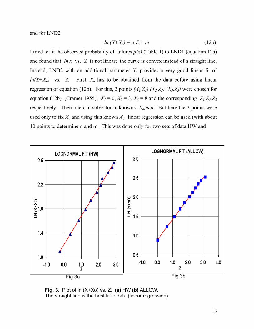
and for LND2

ln (X+Xo) = σ Z + m (12b)

I tried to fit the observed probability of failures p(x) (Table 1) to LND1 (equation 12a)

and found that ln x vs. Z is not linear; the curve is convex instead of a straight line.

Instead, LND2 with an additional parameter Xo provides a very good linear fit of

ln(X+Xo) vs. Z. First, Xo has to be obtained from the data before using linear

regression of equation (12b). For this, 3 points (X1,Z1) (X2,Z2) (X3,Z3) were chosen for

equation (12b) (Cramer 1955); X1 = 0, X2 = 3, X3 = 8 and the corresponding Z1,Z2,Z3

respectively. Then one can solve for unknowns Xo,m,σ. But here the 3 points were

used only to fix Xo and using this known Xo, linear regression can be used (with about

10 points to determine σ and m. This was done only for two sets of data HW and

Fig 3a Fig 3b Fig. 3. Plot of ln (X+Xo) vs. Z. (a) HW (b) ALLCW. The straight line is the best fit to data (linear regression)

16

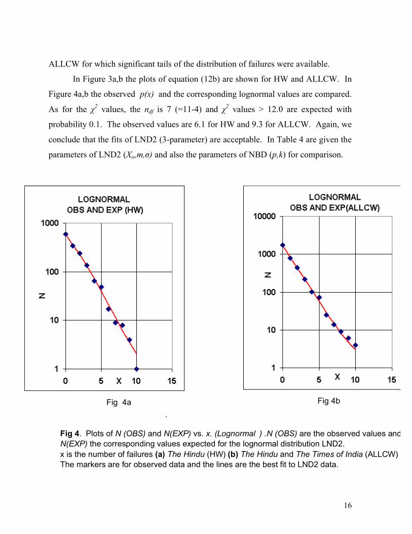
ALLCW for which significant tails of the distribution of failures were available.

In Figure 3a,b the plots of equation (12b) are shown for HW and ALLCW. In

Figure 4a,b the observed p(x) and the corresponding lognormal values are compared.

As for the χ2 values, the ndf is 7 (=11-4) and χ2 values > 12.0 are expected with

probability 0.1. The observed values are 6.1 for HW and 9.3 for ALLCW. Again, we

conclude that the fits of LND2 (3-parameter) are acceptable. In Table 4 are given the

parameters of LND2 (Xo,m,σ) and also the parameters of NBD (p,k) for comparison.

Fig 4a Fig 4b .

Fig 4. Plots of N (OBS) and N(EXP) vs. x. (Lognormal ) .N (OBS) are the observed values and N(EXP) the corresponding values expected for the lognormal distribution LND2. x is the number of failures (a) The Hindu (HW) (b) The Hindu and The Times of India (ALLCW) The markers are for observed data and the lines are the best fit to LND2 data.

17

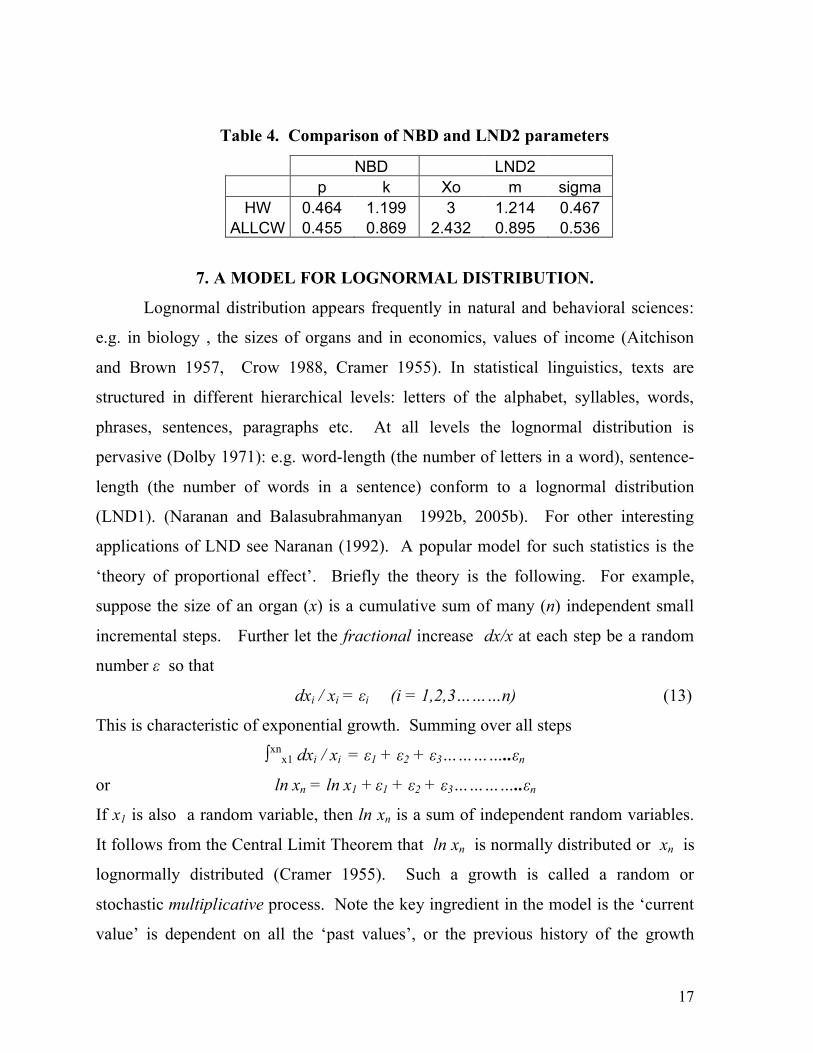
Table 4. Comparison of NBD and LND2 parameters

NBD LND2 p k Xo m sigma

HW 0.464 1.199 3 1.214 0.467 ALLCW 0.455 0.869 2.432 0.895 0.536

7. A MODEL FOR LOGNORMAL DISTRIBUTION.

Lognormal distribution appears frequently in natural and behavioral sciences:

e.g. in biology , the sizes of organs and in economics, values of income (Aitchison

and Brown 1957, Crow 1988, Cramer 1955). In statistical linguistics, texts are

structured in different hierarchical levels: letters of the alphabet, syllables, words,

phrases, sentences, paragraphs etc. At all levels the lognormal distribution is

pervasive (Dolby 1971): e.g. word-length (the number of letters in a word), sentence-

length (the number of words in a sentence) conform to a lognormal distribution

(LND1). (Naranan and Balasubrahmanyan 1992b, 2005b). For other interesting

applications of LND see Naranan (1992). A popular model for such statistics is the

‘theory of proportional effect’. Briefly the theory is the following. For example,

suppose the size of an organ (x) is a cumulative sum of many (n) independent small

incremental steps. Further let the fractional increase dx/x at each step be a random

number ε so that

dxi / xi = εi (i = 1,2,3………n) (13)

This is characteristic of exponential growth. Summing over all steps

∫xnx1 dxi / xi = ε1 + ε2 + ε3…………..εn

or ln xn = ln x1 + ε1 + ε2 + ε3…………..εn

If x1 is also a random variable, then ln xn is a sum of independent random variables.

It follows from the Central Limit Theorem that ln xn is normally distributed or xn is

lognormally distributed (Cramer 1955). Such a growth is called a random or

stochastic multiplicative process. Note the key ingredient in the model is the ‘current

value’ is dependent on all the ‘past values’, or the previous history of the growth

18

process. In contrast a random additive process (i.e. dxi = εi instead of dxi / xi = εi

from equation 13) leads to the normal distribution for xn.

The above model can be suitably modified for the 3-parameter LND2

(equation 10) by postulating

dxi /( xi+Xo) = εi (i = 1,2,3………n) (13a)

to replace equation (13), leading to a lognormal distribution for ( xi+Xo), where X0 is

a constant. This implies dxi is proportional to ( xi+Xo) and not xi ; in other words,

both additive and proportionate effects are in operation.

Does the theory of proportionate effect have any relevance for the distribution

of the number of failures in crosswords, p(x)? There is a feature in the accumulation

of ‘failures’ in a puzzle, which has some resemblance to the proportional effect. The

first failure occurs at random in the grid (x = 1). But when x = 2, the second failure is

more likely to occur in a crossword that intersects the first failure, because it gets no

help from the first failure (which is an unknown word). Similarly when x = 3 the third

failure is more likely to be one of the words intersecting either or both the first and

second failures. It is clear that there is a semblance of proportional effect here

although it is difficult to quantify. The proportional effect is only partial since a new

failure can also occur in a random crossword on the grid. This additive effect may

also contribute to the ‘evolution’ of the number of failures. Observationally too, I

have noticed that failures have a tendency to occur in one or more clusters in the grid.

The LND2 with an extra parameter Xo may be a good way to model this fact.

Admittedly the model is semi-quantitative at best. It is worth citing here an analysis

of the popular board game “Snakes and Ladders”. It is claimed that the number of

moves to reach the end of the game – after ascending the ladders and descending the

snakes – is a lognormal distribution. In this game, it is obvious that the ‘current

position’ of a player on the board depends on all the previous moves, although each

move is decided randomly by throwing a dice.

19

8. COMPARISON OF NEGATIVE BINOMIAL AND LOGNORMAL

DISTRIBUTION MODELS.

It is not often that we find observations that are equally well described by two

different well-known and popular statistical distributions. Here we have the

distribution p(x) of x the number of unsolved clues in a crossword puzzle, satisfying

the ‘goodness of fit of hypothesis’ test – the χ2 test – of two different hypothetical

statistical distributions equally well. They are the 2-parameter NBD and the 3-

parameter LND2. Can we choose one as better than the other? Obviously, the 2-

parameter NBD has one free parameter less than the 3-parameter LND2 for adjusting

the data to theory, and is the preferred one. It is possible that an increase in sample

size NT will help resolve the dichotomy. (I have already mentioned that small

samples of data seem to fit a 2-parameter LND1). But this requires more data from

more solvers.

It appears that LND2 may mimic NBD in a narrow range of values of the

parameters p and k characterizing the NBD. Here we have p ≈ 0.46 and k = 0.9 – 1.2

(Table 4) characteristic of the solver (author). For other values of (p,k) – other solvers

and/or puzzles – the correspondence of NBD and LND2 may not hold. In other

words, NBD may be the only one that is relevant for all puzzles and solvers.

Viewing the same set of observations from two different angles will add to our

understanding of the underlying mechanisms governing them. Both NBD and LND

have wide ranging applications and are well supported by robust theory. Robustness

is also evident in the data since the totality of data (ALLCW) as well as its 4

constituents (HW,HS,TW,TS) all conform to NBD (Tables 2,3). Similarly ALLCW

and its constituent HW both conform to LND2 (Table 4). This suggests that

superposition of multiple sets of data still conforms to the same distribution (NBD

and LND2) that applies to the individual sets.

As regards the modeling of data: NBD offers a straightforward and plausible

interpretation as a mixture of Poisson and Gamma Distributions. For LND2 there is

20

some indication of the applicability of the theory of proportional effect. In summary

the NBD has a clear advantage over the LND2.

9. CONCLUSIONS AND SUMMARY.

I believe the observation on the distribution of the number of unsolved clues in

cryptic crossword puzzles presented here is perhaps unique in behavioral science, e.g.

the puzzle-solving behavior of linguistic puzzles. The sample size of total data (3404)

- gathered over a decade by the author - is substantial enough to examine the tails of

the distribution. Considering that crossword puzzle solving is a major recreational

and intellectual activity in the masses, the study is likely to be important for

understanding the nature of puzzle solving. It is pertinent to note that crossword

puzzle solving is a recommended pursuit for helping ward off dementia in old age.

The investigation is also of linguistic significance since the clues reflect creative and

innovative aspects of word usage in syntactic and semantic sense. For a novice, the

cryptic crossword clues make little sense and even appear ‘insane’ and ‘crazy’. The

composer revels in various tricks of word play: anagrams, puns, reversals, words

nested in words etc. (See for example Sandy Balfour, 2008). In this the British

cryptics differ from their American counterpart. The grids are dense in the American

puzzles and skeletal in the cryptics. There are 70-80 crosswords in a 15 x 15

American puzzle compared to 28 – 34 in cryptic puzzles. The denser packing of

words in the American version is made possible by resorting to words (as solutions)

that are very rare and unfamiliar – most of them not in dictionaries – acronyms etc.

But to compensate for the challenge, the clueing is straightforward unlike the

convoluted and sometimes “Rube-Goldberg” style of clueing in cryptics (Matt

Gaffney 2006).

Language as a tool for communication – its most compelling rationale – is

simple, direct and lucid in normal usage; as a puzzle it is meant to intrigue and

entertain. For the solver it is not only an intellectual challenge, but also enjoyable. At

the other extreme is secret coded communication or cryptography. Simon Singh

21

(2000) alludes to a connection between skills in crossword puzzle solving and code-

breaking (cryptanalysis). In 1942 during the World War II, the British Government

recruited staff for the project to crack the German secret code, the Enigma. One of

the main criteria for eligibility was the ability to completely solve a crossword puzzle

in 12 minutes or less. The British crossword puzzles perhaps derive their popular label

‘cryptic’ from cryptography.

Just as in linguistics there are surprising regularities such as Zipf’s Law of

word frequencies (Zipf 1949, Baayen 2001), in the solving of crossword puzzles too

there are statistical regularities as demonstrated in this article. Both linguistic

discourses and the sets of clues in crossword puzzles are free creations of the mind,

yet they exhibit some regular and universal statistical behavior. Randomness plays an

important role in puzzle solving as exemplified in the NBD model, which is an

extension of the Poisson Distribution characteristic of random counting. This is

interesting because the puzzles themselves are purely games of skill and not chance

and the word solutions to clues are unique.

Many complex systems, well-organized hierarchical structures like a language

text or a DNA sequence for example, exhibit coexisting order and randomness. For a

detailed discussion see Balasubrahmanyan and Naranan (1996, 2005a).

What are the desirable future investigations in crossword puzzle solving? A

large sample size (NT) is crucial for statistical analysis of data with long tails. This

can be achieved in three ways: (A) many crossword puzzles and one solver, (B) one

crossword puzzle and many solvers and (C) many puzzles and many solvers. The

present attempt is an example of (A). To achieve (B), the following is suggested. A

composer of a published puzzle can add a footnote requesting each solver, who tried

to complete the puzzle, to send his number of unsolved clues by SMS to him. The

composer can then make the data collected available to anyone interested in analyzing

it. Repetition of (A) and or (B) will make up category (C). There is a case for an

organized group of solvers undertaking the exercise. With many crossword puzzle

aficionados in long-standing pursuit of the hobby there is great potential for immense

22

volume of statistical data. It will be interesting to see if the American type puzzles

too show similar statistical properties.

In summary, solutions to cryptic crossword puzzle accumulated over a decade

by the author (total sample 3404) yield a probability distribution p(x) of the number

of failures. First the total sample is divided into 4 groups and each analyzed

separately for fit to a statistical distribution. The Poisson Distribution with a single

parameter (λ) is a poor fit to p(x). The Negative Binomial Distribution (NBD), a

generalization of the Poisson Distribution with two parameters (p,k) fits very well all

the sets of data separately and in totality (Table 2,3; Figures 1,2). The pair (p,k) is

characteristic of the solver; in this case the author has (p,k) = (0.455, 0.869). When a

group of puzzles of varying complexity is involved their combined effect on p(x) can

be regarded as yielding a mixture distribution of x, in which a fixed λ is replaced by a

varying λ distributed according to the Gamma distribution.

The p(x) is also equally well fit by a 3-parameter lognormal distribution. For

total data (ALLCW) the three parameters (Xo,m,σ) are (2.42,0.895,0.536). It is

suggested that the dichotomy – two different statistical distributions fitting the same

data – may be true only for a narrow range of (p,k) values. For another solver with

different (p,k) only the NBD may be a valid choice. Further, NBD is the preferred

distribution because it has only 2 free parameters instead of 3. The mixture

distribution model of NBD is a plausible one reflecting reality, whereas the model for

LND based on the theory of proportional effect is somewhat qualitative.

This investigation is new in behavioral science (linguistics, word puzzle

solving) and warrants more data gathering from a group of puzzle solvers. I conclude

with a conjecture that is prompted by the model proposed for the observations

(section 3). Negative Binomial Distribution will prove to be appropriate for all

crossword puzzles and all solvers and therefore universal.

23

Acknowledgement.

When my brother S. Srinivasan learnt about my unusual and very personal

project on crosswords, he convinced me that the results deserved to be shared with the

public. I thank him for his interest and encouragement. I thank my daughter Gomathy

Naranan for a critical reading of the draft manuscript and her suggestions for

improvement.

24

REFERENCES

Aitchison, J. and Brown, J.A.C. (1957). The Lognormal Distribution. Cambridge

University Press, Cambridge.

Baayen, R.H. (2001). Word Frequency Distributions. Dordrecht: Kluwer Academic

Publishers.

Balasubrahmanyan, V.K . & Naranan, S. (1996). Quantitative linguistics and

complex system studies. Journal of Quantitative Linguistics 3, 177-228.

Balasubrahmanyan, V.K. & S. Naranan (2000). Information theory and

algorithmic complexity: Applications to language discourses and DNA

sequences as complex systems: Part II: Complexity of DNA sequences,

analogy with linguistic discourses. Journal of Quantitative Linguistics 7, 153-

183.

Balasubrahmanyan, V.K. & S. Naranan (2005). Entropy, Information and

Complexity. In R. Kohler, G. Altmann, R.G. Piotrowski (Eds.). An

International Handbook of Quantitative Linguistics (pp 878-891). Berlin/New

York: de Gruyter.

Balfour, S. (2008). A Clue to our lives: 85 years of the “Guardian” Cryptic

Crosswords. Gwynedd, UK: Guardian Books.

Boswell, M.T and Patil, G.P. (1970). Chance mechanisms generating the Negative

Binomial Distributions. Retrieved January 5, 2010 from

http://libra.msra.cn/Paper/2822010.aspx.

Cramer, H. (1955). The Elements of Probability Theory and Some of its Applications.

New York/London/Sydney: John Wiley & Sons, Inc..

Crow, E.L. and Shimuzu, K. (Eds.) (1988). Lognormal Distribution: Theory and

Applications. New York: Marcel Dekker.

Dionne, G. and Vanasse, C. (1990) In: Workshop on “A Generalization of

Automobile Insurance Rating Models: The Negative Binomial Distribution

with a Regression Component”. Montreal: University of Montreal.

25

Dolby, J.A. (1971). Programming languages in mechanized documentation. Journal

of Documentation, 27, 136-155.

Ehrenberg, A.S.C. (1988). Repeat Buying: Facts, theory and Applications. Oxford:

Oxford University Press.

Feller, W. (1972). An Introduction to Probability Theory and its applications. Vol. 1.

New Delhi, India: Wiley Eastern Private Ltd.

Gaffney, M. (2005). Gridlock. New York: Thunder’s Mouth Press.

Greenwood, M. and Yule, G.U. (1920). An inquiry into the nature of the frequency

distribution of multiple happenings. Journal of Royal Statistical Society A83,

255-279.

Hilbe, J.M. (2007). Book of Negative Binomial Regression. Cambridge: Cambridge

University Press.

Johnson, P. and Vieux, A. (2006). “Negative Binomial”. Retrieved January 5, 2010

from http://pj.freefaculty.org/stat/Distributions/NegativeBinomial.pdf.

Naranan, S. (1992) Statistical laws in Information Science, Language and system of

Natural numbers: Some striking similarities. Journal of Scientific and

Industrial Research, 51, 736-755.

Naranan, S. and Balasubrahmanyan, V.K. (1992). Information theoretic models in

statistical linguistics. Part II: Word frequencies and hierarchical structure in

language – statistical tests. Current Science, 63, 297-306.

Naranan, S. and Balasubrahmanyan, V.K. (2005). Power laws in statistical

linguistics and related systems. In R. Kohler, G. Altmann, R.G. Piotrowski

(Eds.).An International Handbook of Quantitative Linguistics. 716-738.

Berlin/New York, de Gruyter.

Singh, S. (2000). The Code Book. London: Ted Smart.

Zipf, G.K. (1949). Human behavior and principle of least effort. Reading: Addison-

Wesley.