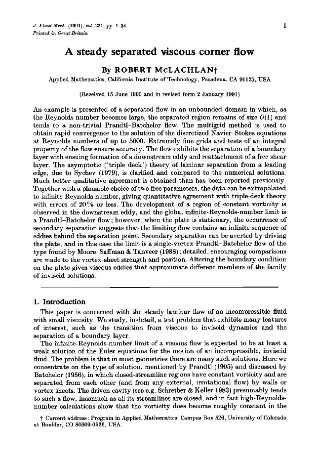
J . Fluid Mech. (1991), vol. 231, p p . 1-34

Printed in areat Britain 1

A steady separated VJscous corner flow

By ROBERT McLACHLANt Applied Mathematics, California Institute of Technology, Pasadena, CA 91 125, USA

(Received 15 June 1990 and in revised form 2 January 1991)

An example is presented of a separated flow in an unbounded domain in which, as the Reynolds number becomes large, the separated region remains of size 0(1) and tends to a non-trivial Prandtl-Batchelor flow. The multigrid method is used to obtain rapid convergence to the solution of the discretized NavierStokes equations at Reynolds numbers of up to 5000. Extremely fine grids and tests of an integral property of the flow ensure accuracy. The flow exhibits the separation of a boundary layer with ensuing formation of a downqtream eddy and reattachment of a free shear layer. The asymptotic ('triple deck') theory of laminar separation from a leading edge, due to Sychev (1979), is clarified and compared to the numerical solutions. Much better qualitative agreement is' obtained than has been reported previously. Together with a plausible choice of two free parameters, the data can be extrapolated to infinite Reynolds number, giving quantitative agreement with triple-deck theory with errors of 20?4 or less. The development,of a region of constant vorticity is observed in the downstream eddy, and the global infinite-Reynolds-number limit is a Prandtl-Batchelor flow ; however, when the plate is stationary, the occurrence of secondary separation suggests that the limiting flow contains an infinite sequence of eddies behind the separation point. Secondary separation can be averted by driving the plate, and in this case the limit is a single-vortex Prandtl-Batchelor flow of the type found by Moore, Saffman & Tanveer (1988) ; detailed, encouraging comparisons are made to the vortex-sheet strength and position. Altering the boundary condition on the plate gives viscous eddies that approximate different members of the family of inviscid solutions.

1. Introduction This paper is concerned with the steady laminar flow of an incompressible fluid

with small viscosity. We study, in detail, a test problem that exhibits many features of interest, such as the transition from viscous to inviscid dynamics and the separation of a boundary layer.

The infinite-Reynolds-number limit 'of a viscous flow is expected to be at least a weak solution of the Euler equations for the motion of an incompressible, inviscid fluid. The problem is that in most geometries there are many such solutions. Here we concentrate on the type of solution, mentioned.by Prandtl (1905) and discussed by Batchelor (1956), in which closed-streamline regions have constant vorticity and are separated from each other (and from any external, irrotational flow) by walls or vortex sheets. The driven cavity (see e.g. Schreiber & Keller 1983) presumably tends to such a flow, inasmuch as all its streamlines are closed, and in fact high-Reynolds- number calculations show that the vorticity does become roughly constant in the

t Current address : Program in Applied Mathematics, Campus Box 526, University of Colorado at Boulder, CO 80309-0526, USA.

2 R. McLachlan

main vortex. However, no Batchelor flows have been calculated in a square (perhaps because of the profusion of walls and vortex sheets!), so detailed comparisons cannot be made. Another candidate for a Batchelor flow as a limit was found by Milos, Acrivos & Kim (1987). In their geometry, straight channels in a periodic array join over a vertical step. For certain values of the ratio of channel widths before and after the step, it appeared that the downstream eddy eventually stopped growing as the Reynolds number increased. Once again, no inviscid calculation has been performed, although it would be easier to do in this case.

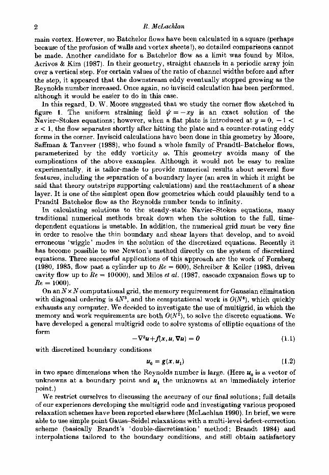
In this regard, D. W. Moore suggested that we study the corner flow sketched in figure 1. The uniform straining field $ = -xy is an exact solution of the Navier-Stokes equations; however, when a flat plate is introduced at y = 0, - 1 < x < 1, the flow separates shortly after hitting the plate and a counter-rotating eddy forms in the corner. Inviscid calculations have been done in this geometry by Moore, Saffman & Tanveer (1988), who found a whole family of Prandtl-Batchelor flows, parameterized by the eddy vorticity w. This geometry avoids many of the complications of the above examples. Although it would not be easy to realize experimentally, it is tailor-made to provide numerical results about several flow features, including the separation of a boundary layer (an area in which it might be said that theory outstrips supporting calculations) and the reattachment of a shear layer. It is one of the simplest open flow geometries which could plausibly tend to a Prandtl-Batchelor flow as the Reynolds number tends to infinity.

In calculating solutions to the steady-state Navier-Stokes equations, many traditional numerical methods break down when the solution to the full, time- dependent equations is unstable. In addition, the numerical grid must be very fine in order to resolve the thin boundary and shear layers that develop, and to avoid erroneous ‘wiggle’ modes in the solution of the discretized equations. Recently it has become possible to use Newton’s method directly on the system of discretized equations. Three successful applications of this approach are the work of Fornberg (1980, 1985, flow past a cylinder up to Re = 600), Schreiber & Keller (1983, driven cavity flow up to Re = lOOOO), and Milos et al. (1987, cascade expansion flows up to Re = 1000).

On a n N x N computational grid, the memory requirement for Gaussian elimination with diagonal ordering is 4N3, and the computational work is O(N4), which quickly exhausts any computer. We decided to investigate the use of multigrid, in which the memory and work requirements are both O ( N 2 ) , to solve the discrete equations. We have developed a general multigrid code to solve systems of elliptic equations of the form

(1.1) with discretized boundary conditions

uo = g(x, u,) (1.2)

-VZu+flx, u, VU) = 0

in two space dimensions when the Reynolds number is large. (Here uo is a vector of unknowns at a boundary point and u1 the unknowns at an immediately interior point.)

We restrict ourselves to discussing the accuracy of our final solutions ; full details of our experiences developing the multigrid code and investigating various proposed relaxation schemes have been reported elsewhere (McLachlan 1990). In brief, we were able to use simple point Gauss-Seidel relaxations with a multi-level defect-correction scheme (basically Brandt ’s ‘ double-discretisation ’ method ; Brandt 1984) and interpolations tailored to the boundary conditions, and still obtain satisfactory

A steady separated viscous corner flow 3

convergence factors (or error reduction per iteration) of 0.34.4. The discrete equations are linearized a t a grid point, and up-wind differencing suppresses quasi- temporal instabilities ; second-order accuracy and artificial-viscosity-free solutions are then restored by defect correction. The small memory requirement (4N2 locations) enables very fine grids to be, used, and the fast relaxations mean that solutions can be obtained in about eight minutes on a workstation (we used a DEC 3100 throughout).

However, we did eventually experience convergence problems, and could not obtain a solution at a Reynolds number of 6000. Although multigrid methods are extremely promising, they are not yet fully understood in all situations.

The corner flow sketched in figure 1 was first studied by Leal (1973), who obtained solutions up to a Reynolds number of 400, based on a reference velocity of 1 and the plate semilength, 1, at which point the eddy still appeared to be fully viscous. In $2, we extend the calculations to a Reynolds number of 5000, and by then the transition to a largely inviscid eddy is clear. Extensive checks of convergence and accuracy are made, including a test of the integral property of the steady-state NavierStokes equations that the total flux of vorticity through a closed streamline is zero. Most flow quantities are accurate to within a few tenths of a percent or less. The development of the flow is described in $3.

In $4 we turn our attention to the primary separation of the flow. The currently accepted explanation of this phenomenon is given by triple-deck theory, first developed using the method of matched asymptotic expansions by Sychev (1972) for separation from bluff bodies, and later extended to the case of separation from a leading edge, as here (Sychev 1979). The flow structure is essentially the same in both cases, except that the expansion proceeds in powers of Re-; in the latter case, rather than Re-&. This makes the proposed effects easier to see. The Sychev model holds that separation is governed by a free interaction.between the boundary layer and the external flow, with the large pressure gradient acting over a small distance being just that required to prevent a singularity. More specifically, the external flow is assumed to be locally a Prandtl-Batchelor flow, which has a singularity in the pressure gradient at separation ; the form of that singularity is then used to derive the scale of the small interaction region. One is left with the standard boundary-layer equation with unusual boundary conditions (the ‘lower-deck problem ’), which was first solved by Smith (1977).

Previous comparisons to triple-deck theory have been either misleading, as in the interaction at the trailing edge of a flat plate (McLachlan 1990, 1991), or have at best indicated that separation is plausibly a local phenomenon (Smith 1977, 1979, 1981). In addition, it is not clear that the appropriate limiting inviscid flow (which supplies two parameters in scaling from the outer variables to the triple deck) has been considered. One notably successful test of modern asymptotics is the work of Dennis & Smith (1980), who considered separation in a tube upstream of a constriction. In that problem separation took place in a fairly large region, of non- dimensionalized streamwise extent O( l), and the small parameter appearing in the asymptotic expansion, Re+, was fortunately small.

We examine the dependence of various flow quantities near separation on the Reynolds number. It is found that the skin friction and the pressure gradient scale almost exactly as predicted by triple-deck theory. This is the best agreement yet obtained (for example, it is not evident in the bluff-body separation results of Fornberg 1985). In addition, the flow profiles are qualitatively similar to the lower- deck solution. Encouraged by this, we next attempt to make a detailed comparison

4 R . McLachlan

by determining the two constants in the theory which are supplied by the global inviscid flow. Apparent quantitative discrepancies can be resolved by considering higher-order terms in the asymptotic expansion.

In the corner flows described in $3, secondary boundary-layer separation at the wall means that the global inviscid limit cannot be one of the one-eddy flows computed by Moore et al. (1988). To sidestep this difficulty, in $5 we change the boundary condition a t the wall to prevent secondary separation. With u(x,O) = up > 0, the reverse boundary layer is accelerated instead of retarded by the wall, and remains attached. This also strengthens the main eddy considerably, causing the emergence of inviscid behaviour in the corner at a lower Reynolds number, and pushes the primary separation point upstream to just ahead of the plate. The eddy now looks almost identical to those of Moore et al. and we make encouraging comparisons of the eddy shapes and the vortex sheet strengths with Prandtl- Batchelor flows. By changing the wall boundary condition, flows with different levels of the constant interior vorticity can be found. We conclude that a simple Prandtl-Batchelor flow is the infinite-Reynolds-number limit in this case.

2. Flow geometry and numerical solution The flow geometry is sketched in figure 1 (a) , and the quadrant in which we solve

the equations in figure 1 (b). The flow is completely specified by the plate, the lines of symmetry on the axes, and the uniform strain in the far field. In the absence of the plate, $ = -xy is an exact solution of the Navier-Stokes equations with velocity u = -x, v = 0 on the x-axis.

We use the stream function-vorticity representation of the flow, in which the velocities are related to the stream function $ by u = $cry, v = - $$ and the vorticity w is defined by w = v,-uy. Non-dimensionalizing lengths by the position of the leading edge, 1, and velocities by the undisturbed velocity at the leading edge, 1, the Navier-Stokes equations for incompressible, steady flow are

VZ$ = - w , ( 2 . 1 ~ )

v 2 w = Re($yW,-$zwy), (2.1 b )

where the Reynolds number Re = 1 / v and v is the kinematic viscosity. Following Leal (1973), we transform to elliptical cylindrical coordinates with x = cosh Ecosq, y = sinhtsinq, in which (2.1) can be written

( 2 . 2 ~ )

(2 .2b )

where J(E,7) = +(cash 25- cos 27) is the Jacobian of the transformation and now V2 = a,+ a,,,,. The quarter-plane x 2 0, y 2 0 maps to the semi-infinite strip E 2 0,O < 7 < in, with the plate at 0 < x < 1, y = 0 mapping to the 7-axis (5 = 0,O < 7 < in).

The x- and y-axes are streamlines so we have $ = 0 there. The symmetry condition is easily written as w = 0. The no-slip condition at the plate, $cry = 0, transforms to $6 = 0.

The boundary conditions in the computational coordinates are

+-xy = -+sinh2(sin27, o+O as t+ 00, ( 2 . 3 ~ )

$&O, 7) = $.CO,q) = 0 for 0 < 7 < in, (2.36)

(2 .3~) $(5,0) = $(& in) = w(5 , 0) = w(6, in) = 0 for 6 > 0.

A steady separated viscous corner $ow 5

\ I / FIGURE 1. Corner flow geometry: (a) entire plane; ( b ) local geometry.

Let the grid spacing be h in the [-direction, and k in the q-direction. Because of the coordinate mapping, the grid spacing on the plate near the leading edge is Ax - i k2 . This concentrates grid points in the region we are interested in, and also reduces the spatial extent of errors caused by the leading-edge singularity. The actual singular point, [ = q = 0, is never used in the relaxations.

The no-slip boundary condition @ - 0 was transformed using the expansion of Woods (1954), in which the surface vorticity is written as a function of the adjacent stream function and vorticity. The Taylor expansions of @ and w with respect to [ are written out at [ = 0, and the first three derivatives of 1cr eliminated using the boundary conditions and (2.2a). This gives

6 -.

n

where wj = w( jh , 7). In some problems, a drawback of this method is that it destroys the expansion of the truncation error in powers of h2 (useful in Richardson extrapolation) which can be obtained using an O(h) approximation for the surface vorticity. However, in solving model problems, (2.4) was found to be much more accurate than other expansions at the values of h used in practice. In any event, the defect correction process will introduce new errors of order h2 and every higher order.

In the far field away from x = 0, the vorticity decays exponentially and we can set w = 0 at [ = 6,. The stream function does not decay exponentially to its free stream value; however, we are fortunate that in this problem it is still sufficient to set $ = -a sinh Z[ sin 27 at [ = 6,. The exponential grid stretching at large [ makes it easy to check the effect of the finite domain; this is shown below to be negligible. Asymptotic boundary conditions are not required.

Close to the y-axis a wake persists, and the vorticity is not exponentially small. It has a similarity form in y % 1 :

w = ay-2g(Reix), g(w) = we-wa/2, (2.5)

where a is a constant. The wake has constant width as y --f rn : the outward diffusion ofvorticity is just balanced by the inward compression of the flow. In the wake we impose the decay w K Y - ~ .

The equations (2.2), together with boundary conditions (2.3) and (2.4), are now in

6 R . McLachlan

Re

150 400

1000 2000 3000 4000 5000

N

160 160 160 320 320 320 320

Vorticity at centre

Coarse Fine Richardson

0.670 0.667 0.666 1.313 1.293 1.285 1.616 1.583 1.572 1.818 1.777 1.762 1.979 1.912 1.889 2.105 2.014 1.984 2.200 2.105 2.074

- Coarse

0.006 0.013 0.058 0.048 0.091 0.148 0.193

Flux error

Fine Richardson

0.004 0.004 0.012 0.007 0.008 0.007 0.019 0.007 0.034 0.006 0.045 0.007

Relative errors in final Re = 5000 solution

Quantity Re-dependence Relative error

1 - Xaep Re0.5 5 x 10-4 "c Re'.3 1.5 x 10-3 7,(xSep 1 Re'.o 1.3 x 10-3 PZ(%,P) Re'." 3 x 10-3 max P z Re'." 3 x 10-2

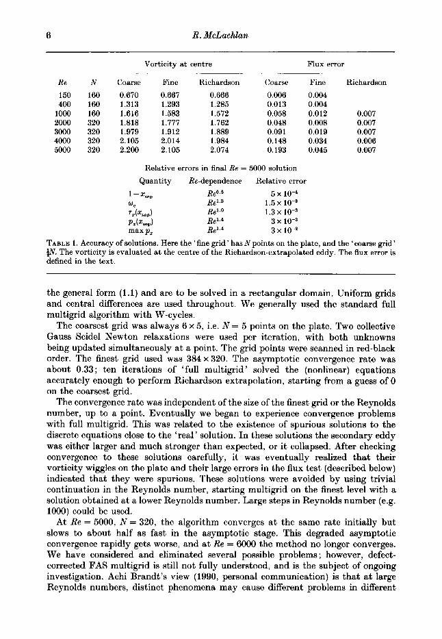
TABLE 1 . Accuracy of solutions. Here the 'fine grid' has Npoints on the plate, and the 'coarse grid' 18. The vorticity is evaluated at the centre of the Richardson-extrapolated eddy. The flux error is defined in the text.

the general form (1 .1) and are to be solved in a rectangular domain. Uniform grids and central differences are used throughout. We generally used the standard full multigrid algorithm with W-cycles.

The coarsest grid was always 6 x 5 , i.e. N = 5 points on the plate. Two collective Gauss-Seidel-Newton relaxations were used per iteration, with both unknowns being updated simultaneously at a point. The grid points were scanned in red-black order. The finest grid used was 384 x 320. The asymptotic convergence rate was about 0.33 ; ten iterations of 'full multigrid ' solved the (nonlinear) equations accurately enough to perform Richardson extrapolation, starting from a guess of 0 on the coarsest grid.

The convergence rate was independent of the size of the finest grid or the Reynolds number, up to a point. Eventually we began to experience convergence problems with full multigrid. This was related to the existence of spurious solutions to the discrete equations close to the 'real' solution. In these solutions the secondary eddy was either larger and much stronger than expected, or i t collapsed. After checking convergence to these solutions carefully, it was eventually realized that their vorticity wiggles on the plate and their large errors in the flux test (described below) indicated that they were spurious. These solutions were avoided by using trivial continuation in the Reynolds number, starting multigrid on the finest level with a solution obtained at a lower Reynolds number. Large steps in Reynolds number (e.g. 1000) could be used.

At Re = 5000, N = 320, the algorithm converges at the same rate initially but slows to about half as fast in the asymptotic stage. This degraded asymptotic convergence rapidly gets worse, and a t Re = 6000 the method no longer converges. We have considered and eliminated several possible problems ; however, defect- corrected PAS multigrid is still not fully understood, and is the subject of ongoing investigation. Achi Brandt's view (1990, personal communication) is that at large Reynolds numbers, distinct phenomena may cause different problems in different

A steady separated viscous corner $ow 7

parts of the flow field, so that to achieve increased performance it will be necessary for the program to recognize the local nature of the flow (e.g. inviscid, a shear layer, or fully viscous) and to take action accordingly.

The errors due to the finite domain are extremely small. At Re = 1000, N = 160, moving the outer boundary from 6, = 1.767 (y, = 2.84) to 6, = 2.356 ( y , = 5.23) changed the reconnection point yrec by only - 2 YO of the discretization error. Accordingly, all runs used 6, = 1.767 for Re > 1OOO.

Originally, we examined the dependence of the solutions on h by repeatedly doubling N and checking that they were in fact second-order accurate. This confirmed that the errors were O(h2) throughout the flow field. In most cases the errors increased faster than the Reynolds number - this is shown in table 1. Since Vw = O(Re) in the boundary layers, and the vorticity transport equation has terms proportional to ReVw, we might expect discretization errors of order O(Re2); fortunately, it appears that these thin layers do not excessively pollute the rest of the solution. However, instead of presenting these results, we concentrate here on a test that checks a known property of incompressible steady flows against the numerical solutions.

The Kirchhoff circulation theorem for steady flow (Batchelor 1967) states that

Vxwds=O ( = ~ [ ~ , V x w d s ’ ) , v.l-c where the integral is taken around any closed streamline ; that is, the total flux of vorticity through any material surface is zero. This conservation law is clearly not built into our numerical solution, so we can use (2.6) to see how well we have satisfied the Navier-Stokes equations globally. We take C to be the contour surrounding the main eddy :

c = u {(x, 0) : 0 < x < xsep,

(0, Y ) Yrec 2 Y 2 0)-

(x, y ) : $(x, y ) = 0 separating streamline,

(2.7)

C‘ is the same contour in the computational coordinates. This includes the entire shear layer, which is where the greatest errors are expected. The entire contour is contained in boundary layers of thickness O(Re-i) (except at its corners), so we expect the local flux of vorticity to be O(Re) - hence the normalizing v in (2.6).

The integral (2.6) is evaluated to second-order accuracy. The position of $ = 0 and ’the flux there are found using linear interpolation from adjacent points. The discretization error incurred in computing the integral is much smaller than that in the integrand. Here the flux of vorticity is directed into the eddy on the separating streamline, and out of the eddy on x = 0 and y = 0. We estimate the relative error as the total flux divided by the absolute flux in or out of the eddy. It would be useful to compare our errors with those in other numerical NavierStokes solutions, but tests such as (2.6) are not frequently applied. Fornberg (1985), in his study of flow past a cylinder, calculated the pressure by integrating along coordinate lines, and found that the error could be up to 9% (at Re = 600) if the path of integration coincided with part of the shear layer ; but his domain was much larger than ours. Carpenter & Homsy (1990) studied a thermally driven flow in a square cavity, also using Newton’s method. They found discrepancies in integral properties of the flow of 3 Yo a t a local Reynolds number of Re I),,, - 300 with h = &.

8 R. McLachlan

(a) Main eddy

Re

150 Leal 400 Leal

1000 2000 3000 4000 5000

x*ep

0.5696 0.58 0.6968 0.70 0.7814 0.8278 0.8497 0.8633 0.8729

Yrec

0.3902 0.39 0.5321 0.515 0.6191 0.6678 0.6908 0.7069 0.7165

YreclX,,p

0.685 0.68 0.764 0.735 0.792 0.807 0.813 0.819 0.821

2,

0.1695

0.1524

0.1524 0.1657 0.1705 0.1755 0.1755

-

-

Y C

0.2010

0.2766

0.2766 0.2337 0.2289 0.2287 0.2287

-

-

*C

0.0031 0.003 0.0083 0.0072 0.0140 0.0182 0.0205 0.0221 0.0234

"c

0.667

1.285

1.572 1.762 1 .889 1.984 2.074

-

-

x c / x * , YCIY* (0.53,0.62) (0.52,0.63) (0.47, 0.62) (0.52,0.63) (0.41, 0.55) (0.39, 0.48) (0.38, 0.45) (0.40, 0.46) (0.39, 0.45)

( b ) Secondary eddy

Re %ep Xrec XC Y c lo4*, WC

- - 0 0 2250 -0.38 - 3000 0.3307 0.4556 0.4055 0.0295 -0.47 -0.347 4000 0.3052 0.4894 0.4239 0.0542 -2.96 -0.760 5000 0.2896 0.5126 0.4371 0.0497 -4.34 -0.733

TABLE 2. Primary eddy characteristics. All data taken from Richardson-extrapolated solutions. $c

and w, are values at the centre of the eddy. See figure 1 ( b ) for more information. Some data from Leal (1973) are included for comparison.

Table 1 gives the flux errors for various mesh sizes and Reynolds numbers. Although (2.6) might accidentally be very small in a particular case, the consistent results indicate that this is not happening, and the relative error is O(h2). Having found these solutions, we bicubically interpolate the coarse-grid solution to the finest grid (introducing small O(h4) errors) and eliminate the leading-order error using Richardson extrapolation, leaving an error of O(h3). (It is essential to know the solution on the finest grid so that the vorticity fluxes can be accurately computed.) The recomputed flux errors are about 0.7 %. Also note that the integrand is the third derivative of the stream function, evaluated in a thin boundary layer, and is expected to have much larger errors than those in ~ and w .

Finally, we have estimated the relative error in our final solution a t Re = 5000, as follows. First the dependence of the errors on Reynolds number was estimated for each quantity. Then the coefficient of h3 in the Richardson-extrapolated solutions was found at Re = 400 (from N = 40, N = 80, and N = 160 calculations), and this result extrapolated to Re = 5000 using the observed power-law dependence. The relative errors are given in table 1 and are mostly a few tenths of a percent. The error is larger in max (p,) because the maximum occurs near the leading-edge singularity, where the finite differences break down.

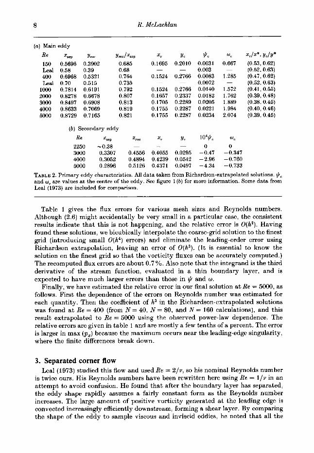
3. Separated corner flow Leal (1973) studied this flow and used Re = 2/v, so his nominal Reynolds number

is twice ours. His Reynolds numbers have been rewritten here using Re = 1 / v in an attempt to avoid confusion. He found that after the boundary layer has separated, the eddy shape rapidly assumes a fairly constant form as the Reynolds number increases. The large amount of positive vorticity generated at the leading edge is convected increasingly efficiently downstream, forming a shear layer. By comparing the shape of the eddy to sample viscous and inviscid eddies, he noted that all the

A steady separated viscous corner $ow 9

\ .- \ -- 1

1 1 -

Re = 400 \ \ \

Y

1 X

0

w

X 1

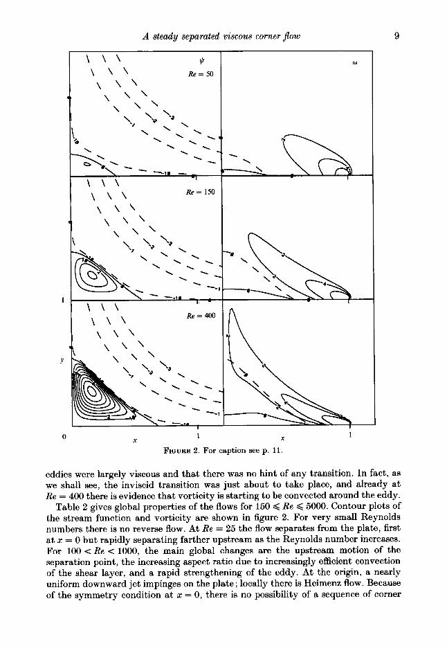
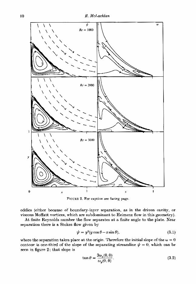
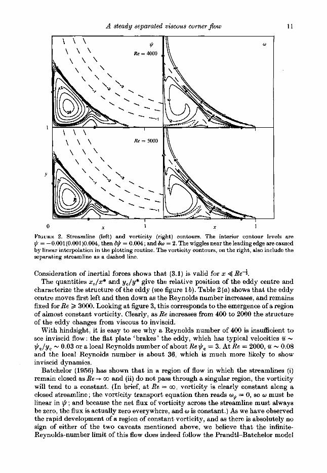
FIGURE 2. For caption see p. 11.

eddies were largely viscous and that there was no hint of any transition. In fact, as we shall see, the inviscid transition was just about to take place, and already a t Re = 400 there is evidence that vorticity is starting to be convected around the eddy.

Table 2 gives global properties of the flows for 150 <Re < 5000. Contour plots of the stream function and vorticity are shown in figure 2. For very small Reynolds numbers there is no reverse flow. At Re = 25 the flow separates from the plate, first at x = 0 but rapidly separating farther upstream as the Reynolds number increases. For 100 <Re < 1000, the main global changes are the upstream motion of the separation point, the increasing aspect ratio due to increasingly efficient convection of the shear layer, and a rapid strengthening of the eddy. A t the origin, a nearly uniform downward jet impinges on the plate; locally there is Heimenz flow. Because of the symmetry condition at x = 0, there is no possibility of a sequence of corner

10 R. McLachlan

1

Y

0 X 1 X 1

FIGURE 2. For caption see facing page.

eddies (either because of boundary-layer separation, as in the driven cavity, or viscous Moffatt vortices, which are subdominant to Heimenz flow in this geometry).

A t finite Reynolds number the flow separates at a finite angle to the plate. Near separation there is a Stokes flow given by

I+ = y2(ycos0-xsin8), (3.1)

where the separation takes place at the origin. Therefore the initial slope of the o = 0 contour is one-third of the slope of the separating streamline @ = 0, which can be seen in figure 2 ; that slope is

A steady separated viscous corner $ow

1

Y

0 X 1 X 1

11

I

FIGURE 2. Streamline (left) and vorticity (right) contours. The interior contour levels are $ = - 0.001 (0.001)0.004, then 8$ = 0.004; and 80 = 2. The wiggles near the leading edge are caused by linear interpolation in the plotting routine. The vorticity contours, on the right, also include the separating streamline as a dashed line.

Consideration of inertial forces shows that (3.1) is valid for x < Re-;. The quantities x,,x* and yJy* give the relative position of the eddy centre and

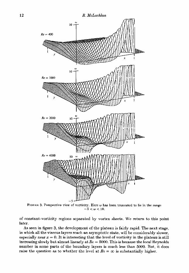
characterize the structure of the eddy (see figure 1 b ) . Table 2 (a) shows that the eddy centre moves first left and then down as the Reynolds number increases, and remains fixed for Re 2 3000. Looking a t figure 3, this corresponds to the emergence of a region of almost constant vorticity. Clearly, as Re increases from 400 to 2000 the structure of the eddy changes from viscous to inviscid.

With hindsight, it is easy to see why a Reynolds number of 400 is insufficient to see inviscid flow : the flat plate ‘brakes ’ the eddy, which has typical velocities ti - @ J y , - 0.03 or a local Reynolds number of about Re $, = 3. A t Re = 2000, ti - 0.08 and the local Reynolds number is about 36, which is much more likely to show inviscid dynamics.

Batchelor (1956) has shown that in a region of flow in which the streamlines (i) remain closed as Re + co and (ii) do not pass through a singular region, the vorticity will tend to a constant. (In brief, a t Re = 00, vorticity is clearly constant along a closed streamline ; the vorticity transport equation then reads wlt = 0, so w must be linear in @; and because the net flux of vorticity across the streamline must always be zero, the flux is actually zero everywhere, and w is constant.) As we have observed the rapid development of a region of constant vorticity, and as there is absolutely no sign of either of the two caveats mentioned above, we believe that the infinite- Reynolds-number limit of this flow does indeed follow the Prandtl-Batchelor model

12 R . McLachlan

FIQURE 3. Perspective view of vorticity. Here w has been truncated to lie in the range -5 < w < 10.

of constant-vorticity regions separated by vortex sheets. We return to this point later.

As seen in figure 3, the development of the plateau is fairly rapid. The next stage, in which all the viscous layers reach an asymptotic state, will be considerably slower, especially near 2 = 0. It is interesting that the level of vorticity in the plateau is still increasing slowly but almost linearly at Re = 5000. This is because the local Reynolds number in some parts of the boundary layers is much less than 5000. But, it does raise the question as to whether the level at Re = co is substantially higher.

A steady separated viscous corner $ow 13

t 1 -0.4 1 I L I I I I

0 0.2 0.4 0.6 0.8 1 .o X

1.2 I I I I

-0.2 I I I I I

0 0.2 0.4 0.6 0.8 1 .o

FIGURE 4 (a, b ) . For caption see next page. X

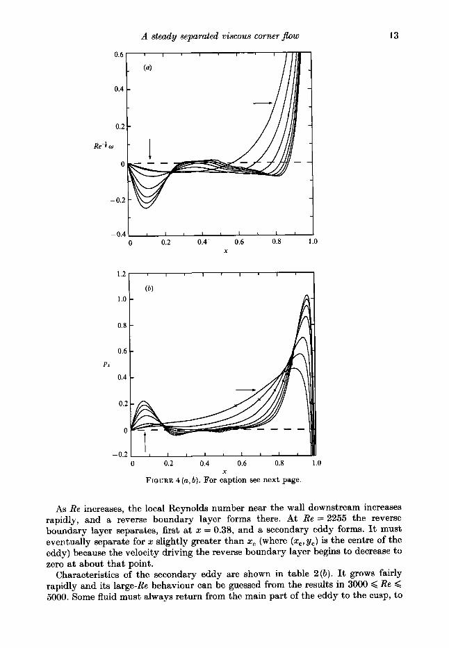
As Re increases, the local Reynolds number near the wall downstream increases rapidly, and a reverse boundary layer forms there. At Re = 2255 the reverse boundary layer separates, first at x = 0.38, and a secondary eddy forms. It must eventually separate for x slightly greater than x, (where (x,, y,) is the centre of the eddy) because the velocity driving the reverse boundary layer begins to decrease to zero at about that point.

Characteristics of the secondary eddy are shown in table 2(b) . It grows fairly rapidly and its large-Re behaviour can be guessed from the results in 3000 <Re < 5000. Some fluid must always return from the main part of the eddy to the cusp, to

14 R. McLachlan

U

0.6

0.4

0.2

0

-0.2

-0.4 I I I I I I

0 0.2 0.4 0.6 0.8 1 .o X

0.2

0.1

Re-' w,

0

-0.1 I I I I I

0 0.2 0.4 0.6 0.8 I .o Y

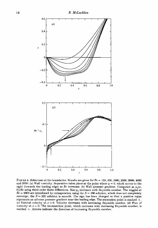
FIGURE 4. Behaviour at the boundaries. Results are given for Re = 150,400, 1000,2000,3000,4000 and 5000. ( a ) Wall vorticity. Separation takes place at the point where w = 0, which moves to the right (towards the leading edge) as Re increases. ( b ) Wall pressure gradient. Computed as wy(x, O)/Re using third-order finite differences. Max p , increases with Reynolds number. The wiggles a t Re = 5000 are introduced by extrapolation using the N = 160 solution, which does not completely converge; the N = 320 solution is smooth. The sign has been changed so that a positive value represents an adverse pressure gradient near the leading edge. The separation point is marked x . (c) Vertical velocity at x = 0. Velocity decreases with increasing Reynolds number. ( d ) Flux of vorticity at x = 0. The reconnection point, which increases with increasing Reynolds number, is marked x . Arrows indicate the direction of increasing Reynolds number.

A steady separated viscous corner flow 15

supply the mass entrained by the shear layer. It appears, though, that as the secondary eddy grows, this return takes place in an O(Re&) shear layer next to the main, outgoing one. Interestingly, all the calculations show a third, weak centre in this layer ; possibly it disappears as Re --f 00 . Velocities are very small, about 0.03, in the region between separation and the secondary reconnection, but it seems inevitable that a tertiary eddy will form there eventually. (A flattening of w in this region is already evident at Re = 5000; see figure 4a.) The inviscid limit would thus consist of an infinite sequence of eddies behind the separation point, each one containing still finer structure. The rapidly decreasing velocities mean that the number of eddies will grow very slowly with the Reynolds number, probably logarithmically.

The separation of the boundary layer will be discussed in detail in $4. With increasing Reynolds number, the reconnection point continues to increase, but the aspect ratio of the eddies levels off sharply once inviscid behaviour has set in. Figure 4 (a) shows the vorticity a t the wall (proportional to shear stress) divided by Re;, the expected asymptotic growth for a simple boundary layer. Although the scaled value is roughly O( l ) , the boundary layer is still developing at Re = 5000. Note that the incipient secondary separation is already hinted at Re = 400: w has a local maximum. The pressure gradient in the boundary layer (equal to the flux of vorticity at the wall divided by Re) is shown in figure 4 ( b ) . There is a Carrier-Lin (1948) singularity at the leading edge, followed by an adverse pressure gradient that increases slowly with Reynolds number, falling to near zero behind separation. Figure 4(c) shows the vertical velocity (v = 0 corresponding to reconnection), and 4(d) the scaled vorticity flux (or p, ) at x = 0. They are still changing at Re = 5000 because the shear layer has diffused considerably by the time it reaches the y-axis.

We note that figures 4(c) and 4(d) are strongly supportive of a triple-deck-like interaction as the smallest scale phenomenon at reconnection, as suggested by Daniels (1979). The vertical velocity gradient vy at separation is proportional to Re0.31, and the scaled vorticity flux to Re0*O6, both exponents being close to their triple-deck values off and i, respectively. However, yrec increases only slowly : if we assume that the inviscid flow reconnects at y = 1, then 1 -ysep K Re-0.'76. This is believed to be due to a relatively large-scale inviscid interaction caused by the shear layer, which rapidly broadens as it nears reconnection. A fully self-consistent description of reconnection has not yet been found. Some discussion of reconnection in free-streamline flows can be found in Cheng & Smith (1982), Cheng (1984), and Cheng & Lee (1985), and an overview in F. T. Smith (1986). The numerical results clearly suggest that it is possible for the shear layer to reattach in an orderly fashion.

J. H. B. Smith (1986) reviews the possibility of a Prandtl-Batchelor limit of a viscous flow. He points out that in many geometries (such as most external and grooved-channel flows) there are serious objections to this model. Our flow was designed to be extremely likely to have an O(1) eddy as Re +- 00 and therefore be a candidate for an external flow with a Prandtl-Batchelor limit.

A family of rotational corner flows was found by Moore et al. (1988, hereinafter referred to as MST), which had internal vorticity 0 < w < 6.11+. (One member of this family was first found by Chernyshenko 1984.) The corresponding flow separating at x = L, say, would have vorticity w and would reconnect at y = L, since only symmetric eddies were found to exist. If such a flow is to be the limit of viscous flow as Re --f 00, the viscous flow would presumably have a core of constant vorticity, with thin O(Re-i) boundary layers near the walls to satisfy the extra boundary condition not present in inviscid flow, and with the vortex sheet being replaced by a shear layer

16 R. McLachlan

0.9

0.8 1, 0.7

0.6

y 0.5

0.4

0.3

0.2

0.1

0 0.1 0.2 0.3 0.4 0.5 0.6 0.7 0.8 0.9 1.0 1.1 X

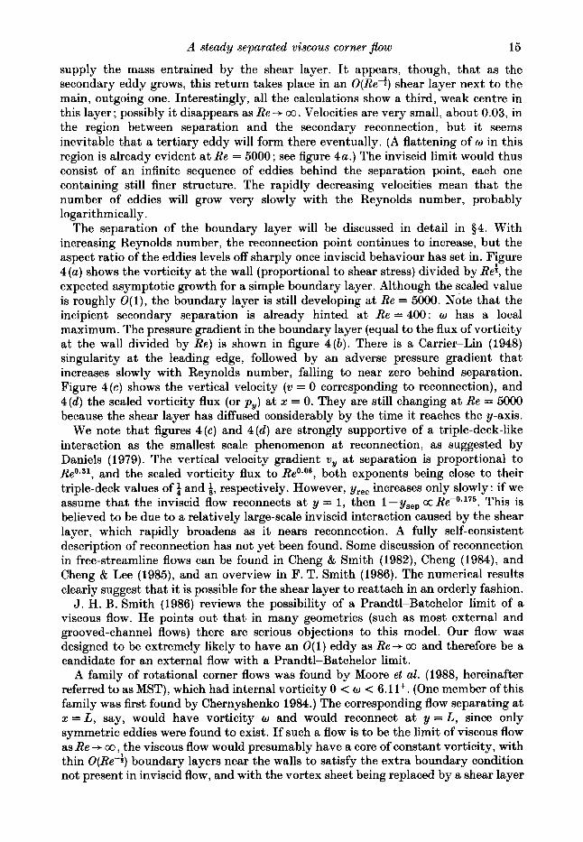
FIQURE 5. Separating streamlines in a corner eddy. The inner solid line is the $ = 0 streamline at Re = 1O00, and the outer line is $ = 0 at Re = 5000. The dashed lines are inviscid vortex-sheet positions, as explained in the text.

with velocity jump y. L and w would then be determined by the wall boundary conditions.

The flow discussed here shows a transition to a largely inviscid eddy that cannot, however, be an MST vortex, because of the finite-sized secondary separation. There are probably more inviscid solutions, consisting of several regions of constant vorticity, each bounded by a vortex sheet. This certainly breaks the symmetry of the 1-region family. However, there is no reason to suppose that tertiary separation is avoided either, which in principle can give rise to an infinite sequence of eddies in the cusp, as suggested by Messiter (1975). Since u(x, 0) = o(1 -x), the Reynolds number necessary to form each successive eddy would increase. This sequence could terminate if the velocity in the cusp decreased with increasing Reynolds number, but this is not indicated by the Re = 5000 results.

Despite these problems, the eddy shapes are rather similar to the MST vortices. Figure 5 shows the separating streamline at Re = 1000 and 5000, compared to the MST vortex with constant vorticity 2 separating a t the same position as the viscous flow. At Re = 1000, the flow near separation is different, but a t Re = 5000 the agreement is encouraging, and surprising in view of the secondary separation - although the secondary eddy may interfere with the external flow as it continues to grow in strength. Certainly the difference is less than the thickness of the shear layer.

Batchelor (1967, plate 7) includes a photograph of an experiment in which a splitter plate is introduced in front of a stagnation point. The main changes from our flow are that the free stream has uniform flow, rather than uniform strain, and that there is also a wall at x = 0, apparently extending to y = 0.55. The Reynolds number is not given. The similarity with our flows is striking. The experimental flow appears to separate at x = 0.81, and the eddy centre in the top eddy is a t x, = 0.23, yc = 0.13 - less than our value because of the different oncoming flow. Secondary separation occurs at x = 0.33. These values suggest that the Reynolds number is between 1000 and 2000. However, there are two strong secondary eddies in y > 0 and several weaker ones, in contrast to our results. Because there is not exact symmetry between

A steady separated viscous corner jlow 17

the two halves of the flow, we believe that these eddies are due to unsteadiness. There may well exist time-periodic flows there in which a sequence of secondary eddies appears a t much smaller Reynolds numbers than in our steady flows.

This idea is supported by the calculations of PQpin (1990) of the flow past an impulsively started cylinder. There, secondary separation has already occurred a t Re = 550. At Re = 3000 two more separations (regions of locally reversed flow) appear when the cylinder has been displaced by 2.75 radii, but these disappear as time increases. Unsteady flows thus appear to be much more susceptible to separation than steady ones.

4. Laminar separation from a leading edge The importance of steady laminar massive separation, in which the disturbance to

the external flow changes from thickness O(Re-5) upstream to O(1) downstream, was first realized by Prandtl (1905). The triple-deck description of this process was developed by Sychev in 1972 for separation from a bluff body, and in 1979 for separation from the leading edge of a flat plate. The latter paper contains an error in the final scaling of the lower-deck equations, which results in an incorrect prediction of which properties of separation are fixed locally and which are supplied by the external flow. We give the correct result below.

We do not reproduce the complete matched asymptotic expansion here; for details, see the Sychev papers, the review by Stewartson (1974), or McLachlan (1990a). J. H. B. Smith (1982, 1986) has reviewed this problem and many more modern applications of high-Reynolds-number theory.

The basic problem in incompressible, large-Reynolds-number flows is that the limiting inviscid solution is not known. Usually there are many solutions that fit the boundary conditions. Which one is selected in the limit Re -+ co remains (except in a few simple cases) an open question. However, the most promising candidate in our case is a Prandtl-Batchelor flow. Although the one-eddy model is not correct for the stationary plate, the global shape does seem to be roughly correct.

Two aspects of the inviscid solution are used in deriving the asymptotic theory. One is the local form of the separating streamline. This will not be affected by changes in the downstream eddy, such as asymmetry or more complicated structure (although certain coefficients could change). The other is the flow in the cusp just behind separation, which supplies a boundary condition for the triple deck. This is discussed below.

In a Prandtl-Batchelor flow separating at x = xsep, the pressure gradient in the inviscid solution just ahead of that point is given by

p , - c(xSep - x)+ as x + xiep. (4.1)

The constant c cannot be negative or zero, because some adverse pressure gradient is required for separation to take place; but c > 0 and an unbounded gradient appears to imply separation upstream of xsep, a contradiction. In the case of bluff- body separation, the resolution is that c is positive but tends to zero as Re +. 00 - it turns out to be O(Re-h). However, in leading-edge separation (Sychev 1979), there is no contradiction because the separation point can move up to the leading edge as Re + co ; c is then a positive constant determined by the global geometry.

Thus, in contrast to the bluff-body case, where c is given by triple-deck theory and the dependence of xsep on c by inviscid theory (e.g. as in Brodetsky 1923), here xSep is determined once c is supplied.

18 R. McLachlan

V

FIGURE 6. Flow structure near separation. I. Lower deck - viscous boundary-layer equations hold. 11. Middle deck - inviscid, vorticity present. 111. Upper deck - inviscid, linearized Euler equations hold. IV. Blasipls boundary layer. V. External inviscid flow. VI. Fully viscous - Navier-Stokes equations hold.

The local flow situation is sketched in figure 6, along with the various regions of the flow in which distinct approximations to the Navier-Stokes equations are valid. The small, fully viscous region at the leading edge has a purely local effect and will not be considered further here. The leading edge is situated a t x = 0. Conventionally, the speed of the external flow is taken to be positive, so that the x-coordinate of 52 must be reversed.

Let v be the kinematic viscosity, and suppose that lengths have been non- dimensionalized by a characteristic length I, velocities by a characteristic undisturbed speed Urn, and pressure pV,. Then the relevant Reynolds number is Re = Urn I l v , and our results will be expressed in terms of the same quantities that are computed numerically.

The leading-order outer solution is taken as a Prandtl-Batchelor flow separating at xSep. However, we assume that the change in its behaviour from the equivalent flow separating a t the leading edge is a higher-order correction, and use the properties of the latter.

Let U, be the velocity of the external flow a t the leading edge. It is initially unknown, since the upstream flow is affected by the (also unknown) eddy shape. It will probably be less than the undisturbed velocity U,. For example, Uo = $ for the irrotational corner eddy. The inviscid pressure gradient and separating streamline are given by

Define

Other authors have used a Reynolds number based on the local free-stream speed U,. However, U, is not known a priori, and i t seems desirable we should a t least know the small parameter.

The scalings of variables in the lower deck (region I in figure 6) are

(4.4)

u = EU = Eqp-IU, = E 3 V = €3qP-tV,

p = $pI = &p+p-$p,

x-xsep = e4X' = e4u-t ?I. y = E S U ' = &,l;%puty,

0

O P

where p = (0112~). Here primed coordinates can be calculated directly from the

A steady separated viscous corner jlow 19

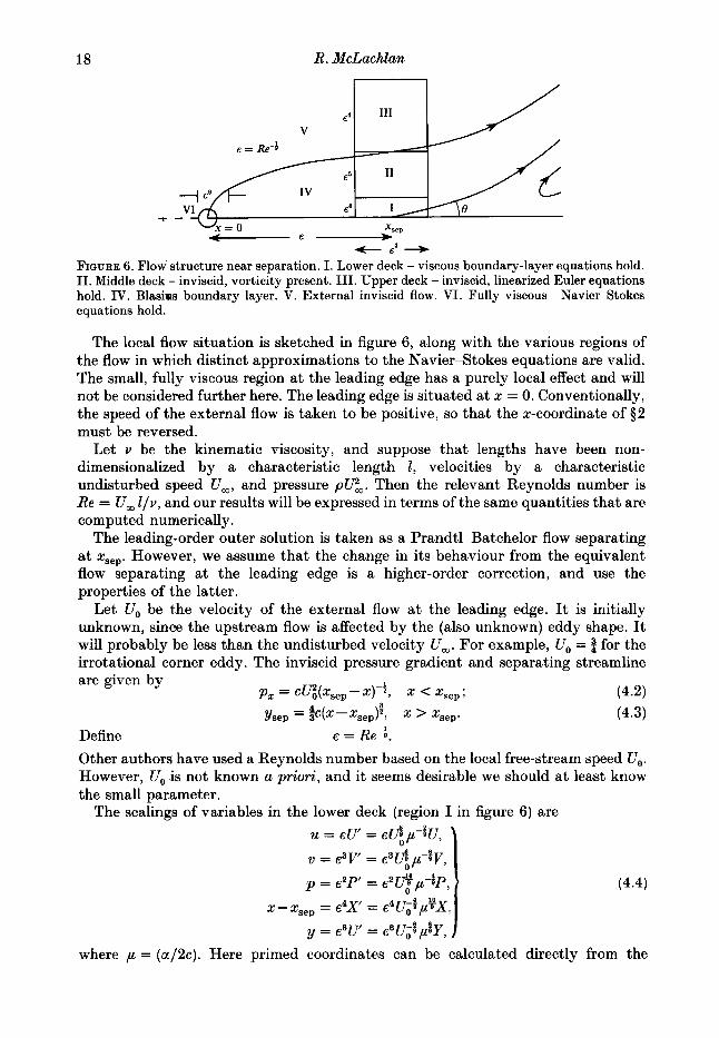
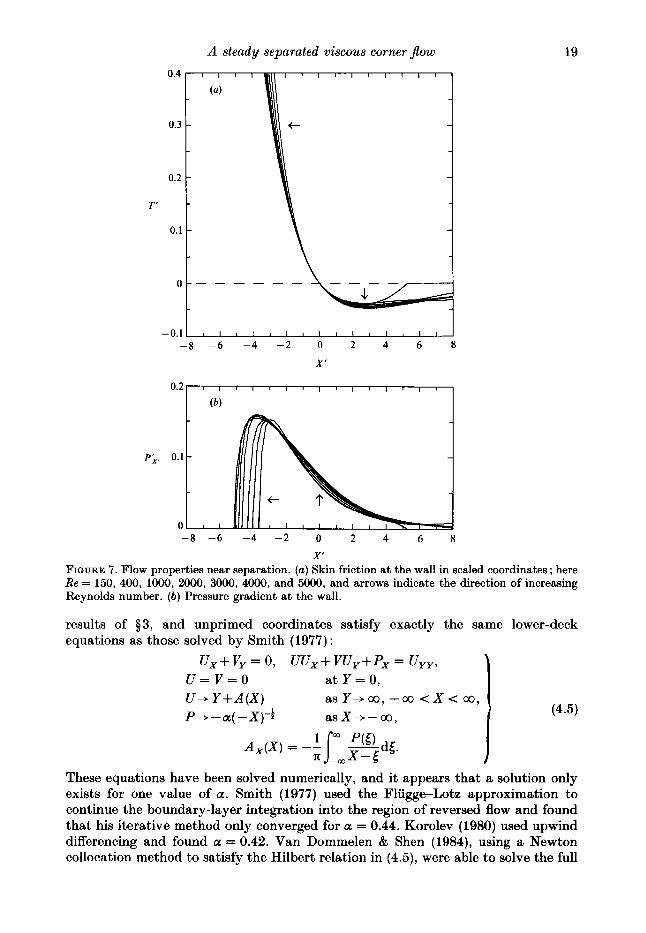
-8 -6 -4 -2 0 2 4 6 8

X' FIGURE 7. Flow properties near separation. (a) Skin friction at the wall in scaled coordinates ; here Re = 150, 400, 1000, 2000, 3000, 4000, and 5000, and arrows indicate the direction of increasing Reynolds number. ( b ) Pressure gradient at the wall.

results of $3, and unprimed coordinates satisfy exactly the same lower-deck equations as those solved by Smith (1977) :

(4.5)

ux+vy = 0, UUX+VU,+PX = uyy, u=v=o at Y = 0, u+ Y + A ( X ) P + -a( -X)- i asX+-co,

as Y + co, - co < X < 00,

These equations have been solved numerically, and it appears that a solution only exists for one value of a. Smith (1977) used the Flugge-Lotz approximation to continue the boundary-layer integration into the region of reversed flow and found that his iterative method only converged for a = 0.44. Korolev (1980) used upwind differencing and found a = 0.42. Van Dommelen & Shen (1984), using a Newton collocation method to satisfy the Hilbert relation in (4.5), were able to solve the full

20 R. McLachEan

equations directly for a, giving a = 0.415. (We use u = 0.42 throughout.) The lower- deck problem is thus regarded as solved.

These three solutions are all qualitatively similar and are summarized in table 3. Unfortunately, in some quantities which we would like to evaluate, they disagree with one another substantially.

The asymptotic distance to separation is

where a, = 0.3321. The presence of vorticity in the limiting flow does not appear to alter asymptotic

structure outlined above. Inviscid considerations were discussed by J. H. B. Smith (1982). In the external flow, the addition of a flow with vorticity is subdominant a t separation to the irrotational flow ; in the cusp, although vorticity gives a different matching condition, the final result (4.3) for the separating streamline is unaltered. The cusp is too small for vorticity to have a local effect.

Consider an inviscid flow with internal vorticity wo and external vorticity w l . When viscosity is present, the change in velocities in the main deck ahead of separation is O(w, y) = O(e5), much smaller than the O(e*) perturbations induced by the free interaction. Downstream, typical velocities inside the wedge 0 < y < ysep = O ( ( x - z , , , ) ~ ) are O(wo ysep). In the irrotational theory, there is a slow return flow near the wall of magnitude O ( B ~ ( X - X ~ , ~ ) - ~ ) . (This is required to supply the mass for the outgoing shear layer; details are in Sychev 1979). Comparing these two quantities, it is clear that the latter becomes dominant well before the interaction region x- x,,, = O(e4) is reached. Thus, vorticity in the cusp does not alter the matching procedure of the triple deck.

In our case, and apparently in all cases of massive steady separation, secondary eddies appear downstream. These may alter U, and c slightly, but their main effect is on the downstream matching of the triple deck. We believe that there is no local change: velocities in the cusp are always extremely small, and because the return flow required by the triple deck is accelerating, it will dominate any effect which tends to zero in the cusp, There could, however, be a change farther downstream, in a region in which these two effects are of the same order.

Previous comparisons of the incompressible triple deck with experiments or calculations have found that, while separation was plausibly a local phenomenon, there was no numerical agreement in detail. Smith (1979, 1981) compares the behaviour at separation with experiments (up to Re = 50) and calculations (up to Re = 300). The results are consistent with the theory but the crucial dependence of scales and quantities on the Reynolds number cannot be determined. (Explanations of larger-scale features of the flow are much more successful.)

For example, in Fornberg’s (1985) calculation of uniform flow past a cylinder up to Reynolds number 600 (based on cylinder diameter), the skin friction a t separation behaves roughly like Reo.ss, instead of the bluff-body triple-deck dependence Re:; and the pressure gradient at separation actually decreased over the entire range of Reynolds numbers considered, roughly like instead of the gradual Re: increase expected. (We have estimated these results from graphs in Fornberg 1985.) Numerical comparisons are difficult because the limiting flow is unknown. In a bluff- body flow, one might take U, = 1 as in the Kirchhoff-Helmholtz model ; and Smith (1979) calculates the extra parameter (the scaled skin friction A ) in this case. However, in a Prandtl-Batchelor flow, U,, A, and the limiting separation point are determined by the vorticity in the eddies; from a local point of view, we have two free parameters.

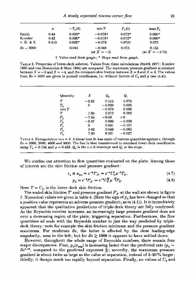
A steady separated viscous corner j o w 21

a -T,(O) min T PX(0) max Px

Korolev 0.42 0.036* -0.078t 0.072* 0.086* v. D. & S. 0.415 0.025* -0.079 0.072t 0.075

Re = 5000 - 0.045 -0.048 0.075 0.155

Smith 0.44 0.033* -0.079t 0.073* 0.090*

(at X = -3) (at X' = -3.75)

t Value read from graph ; * Slope read from graph.

TABLE 3. Properties of lower-deck solution. Values from three calculations (Smith 1977 ; Korolev 1980 and van Dommelen & Shen 1984) are compared. The maximum pressure gradient is attained between X = -3 andX = -4, and the minimum skin friction between X = 6 and X = 8. The values from Re = 5000 itre given in primed coordinates, i.e. without factors of Uo and p (see (4.4)).

Quantity X QO Qi

T -3.82 0.113 0.078 TX 0 -0.030 0.025 min T -0.078 0.092 T 7.65 0.072 0.082 P X -7.65 -0.08 > O PX -3.82 0.099 -0.039 P X 0 0.091 -0.107 P X 3.82 0.049 -0.065 P X 7.65 0.021 -0.027

TABLE 4. Extrapolation to E = 0. A linear best fit was made of various quantities against E , through Re = 2000, 3000, 4000 and 5000. The line is then transformed to standard lower-deck coordinates using Uo = 0.734 and ,u = 0.493. Qo is the E = 0 intercept and Q, is the slope.

We confine our attention to flow quantities evaluated on the plate. Among those of interest are the skin friction and pressure gradient :

Here T = U, is the lower-deck skin friction. The scaled skin friction T' and pressure gradient Pk, at the wall are shown in figure

7. Numerical values are given in table 4. (Here the sign ofpx has been changed so that a positive value represents an adverse pressure gradient, as in (4.1)). It is immediately apparent that the qualitative predictions of triple-deck theory are fully confirmed. As the Reynolds number increases, an increasingly large pressure gradient does act over a decreasing region of the plate, triggering separation. Furthermore, the flow quantities all scale with the Reynolds number in just the way predicted by triple- deck theory : note for example the skin friction minimum and the pressure gradient maximum. For moderate Re, the latter is affected by the close leading-edge singularity, seen to the left; but for Re 2 lo00 it appears to have settled down.

However, throughout the whole range of Reynolds numbers, there remain four major discrepancies. First, px(xSep) is increasing faster than the predicted rate (p, - ReQ.34 , compared to the predicted exponent 3 ) ; secondly, the maximum pressure gradient is about twice as large as the value at separation, instead of 5-20 YO larger ; thirdly, it decays much too rapidly beyond separation. Finally, no values of UQ and

22 R. McLachlan

0.4 c I I I I I 1 I I I I

0 0.1 0.2 0.3 0.4 0.5 0.6

E = Re-i

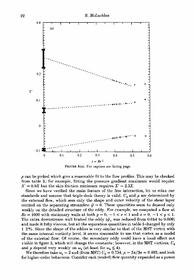
FIGURE 8(a) . For caption see facing page.

p can be picked which give a reasonable fit to the flow profiles. This may be checked from table 3; for example, fitting the pressure gradient maximum would require X = 0.9X but the skin-friction minimum requires X' = 2.3X.

Since we have verified the main feature of the free interaction, let us relax our standards and assume that triple-deck theory is valid. lJo and p are determined by the external flow, which sees only the shape and outer velocity of the shear layer centred on the separating streamline $ = 0. These quantities seem to depend only weakly on the detailed structure of the eddy. For example, we computed a flow a t Re = 1000 with stationary walls a t both y = 0, - 1 < x < 1 and x = 0, - 1 < y < 1. The extra downstream wall braked the eddy ($c was reduced from 0.014 to 0.009) and made i t fully viscous, but all the separation quantities in table 5 changed by only 1-2 %. Since the shape of the eddies is very similar to that of the MST vortex with the same internal vorticity level, it seems reasonable to use that vortex as a model of the external flow. Of course, the secondary eddy could have a local effect not visible in figure 5, which will change the constants ; however, in the MST vortices, Uo and p depend very weakly on wo (at least for wo 5 4).

We therefore take wo = 2 and (from MST) U, = 0.734, p = 2a/3a = 0.493, and look for higher-order behaviour. Consider each (scaled) flow quantity expanded as a power

A steady separated viscous corner $ow 23

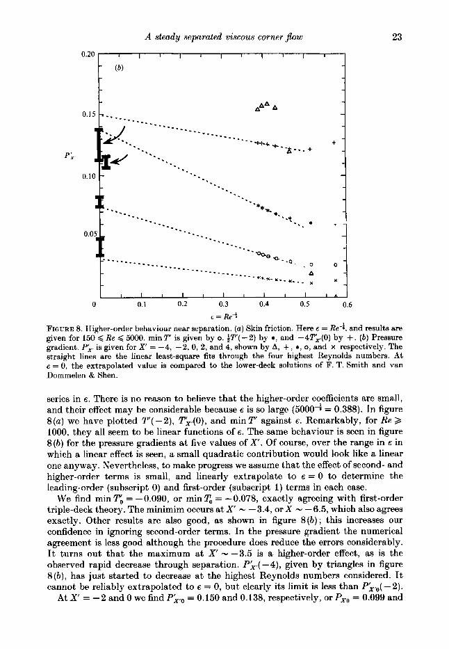
0.20 I I I I I I I I I I I I

0.10 t

. * - - - - .- I- -..

... ... .... '*.

..... ._ -. + -.

O . O I . . .......

*

0

A ' X

I I I I I I I I I I I I *

0 0.1 0.2 0.3 0.4 0.5 0.6

FIGURE 8. Higher-order behaviour near separation. (a) Skin friction. Here E = Re-:, and results are given for 150 < Re < 5000. minT is given by 0. tT( -2) by *, and -4T'.(O) by +. (a) Pressure gradient. Px, is given for X' = -4, - 2 , O , 2, and 4, shown by A, +, *, 0, and x respectively. The straight lines are the linear least-square fits through the four highest Reynolds numbers. At E = 0, the extrapolated value is compared to the lower-deck solutions of F. T. Smith and van Dommelen & Shen.

= Re-!

series in e. There is no reason to believe that the higher-order coefficients are small, and their effect may be considerable because e is so large (5000-i = 0.388). In figure 8 ( a ) we have plotted T(-2) , Tx(0), and minT against e. Remarkably, for Re > 1000, they all seem to be linear functions of e. The same behaviour is seen in figure 8 ( b ) for the pressure gradients at five values of X . Of course, over the range in e in which a linear effect is seen, a small quadratic contribution would look like a linear one anyway. Nevertheless, to make progress we assume that the effect of second- and higher-order terms is small, and linearly extrapolate to E = 0 to determine the leading-order (subscript 0) and first-order (subscript 1) terms in each case.

= -0.078, exactly agreeing with first-order triple-deck theory. The minimim occurs at X - -3.4, orX - -6.5, which also agrees exactly. Other results are also good, as shown in figure 8 ( b ) ; this increases our confidence in ignoring second-order terms. In the pressure gradient the numerical agreement is less good although the procedure does reduce the errors considerably. It turns out that the maximum at X - -3.5 is a higher-order effect, as is the observed rapid decrease through separation. P>,( -4), given by triangles in figure 8 ( b ) , has just started to decrease at the highest Reynolds numbers considered. It cannot be reliably extrapolated to E = 0, but clearly its limit is less than - 2).

A t x' = -2 and 0 we find Px,o = 0.150 and 0.138, respectively, or P,, = 0.099 and

We find min To = -0.090, or min

24 R. McLmhlan

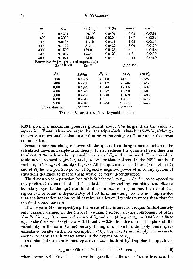
Re Xsep -7z(xsep)

150 0.4304 6.106 400 0.3032 15.96

1000 0.2185 41.12 2000 0.1722 84.44 3000 0.1503 129.9 4000 0.1367 175.7 5000 0.1271 223.0

Power-law fit [us. predicted exponents] Re-0.34 [-1/91 Re1.05 I11

Re

150 400

1000 2000 3000 4000 5000

Power-law fit:

Pz(Xsep)

0.1828 0.2298 0.2999 0.3693 0.4208 0.4618 0.4978

Re0.34 [2/91

- T ( O )

0.0407 0.0399 0.041 1 0.0422 0.0433 0.0439 0.0446

P X W 0.0600 0.0607 0.0646 0.0682 0.0710 0.0731 0.0750

min 7

-0.63 - 1.07 -1.92 -3.00 -3.91 -4.81 - 5.45

max P z

0.4651 0.5745 0.7005 0.8628 0.9459 0.9951 1.0261

Re0.24 [2/91

TABLE 5. Separation at finite Reynolds number

min T

-0.0391 -0.0384 -0.0413 -0.0439 -0.0458 -0.0479 -0.0480

max P x

0.1527 0.1517 0.1509 0.1593 0.1596 0.1575 0.1546

0.091, giving a maximum pressure gradient about 9% larger than the value a t separation. These values are larger than the triple-deck values by 15-25 %, although this error is much smaller than in our first-order matching. At X' = 2 and 4 the errors are much less.

Second-order matching removes all the qualitative disagreements between the calculated flows and triple-deck theory. It also reduces the quantitative differences to about 20% or less when plausible values of U, and ,LA are used. This procedure could never be used to Jind U, and ,LA (or a, for that matter). In the MST family of vortices, dU,/dw, < 0 and dp/dw, < 0. All the quantities of interest (see (4.4), (4.7) and (4.8)) have a positive power of U, and a negative power of p, so any system of equations designed to match them would be very ill-conditioned.

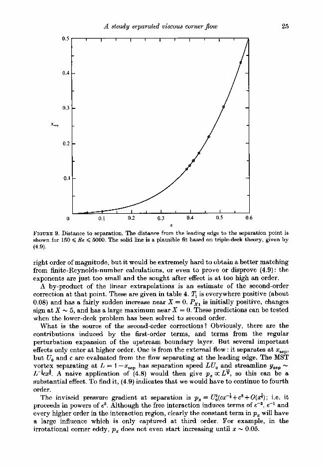
The distances to separation (see table 5 ) behave like xsep - Re-0.34, as compared to the predicted exponent of -0. The latter is derived by matching the Blasius boundary layer to the upstream limit of the interaction region, and the size of that region can be found independently of that final matching. So it is not implausible that the interaction region could develop at a lower Reynolds number than that for the final behaviour (4.6).

If we regard (4.6) as specifying the onset of the interaction region (unfortunately only vasuely defined in the theory), we might expect a large component of order X = Re-3 in xSep. Our assumed values of U, and p in (4.6) give xsep = 0.0325s. A fit to zSep of the form as+ be4 gives a = 0.14 and b = 3.26, but this does not explain all the variability in the data. Unfortunately, fitting a full fourth-order polynomial gives unrealistic results (with, for example, a < 0). Our results are simply not accurate enough to capture this many terms in the expansion of xsep.

One plausible, accurate least-squares fit was obtained by dropping the quadratic term :

where Jerrorl < 0.0004. This is shown in figure 9. The linear coefficient here is of the

xSep = 0.0501s+ 1 .2042e3 + 1 .6244~~ +error, (4.9)

A steady separated viscous corner $ow 25

0.5

0.4

0.3

xsep

0.2

0.1

0 0.1 0.2 0.3 0.4 0.5 0.6

FIGURE 9. Distance to separation. The distance from the leading edge to the separation point is shown for 150 < R e < 5000. The solid line is a plausible fit based on triple-deck theory, given by (4.9).

6

right order of magnitude, but it would be extremely hard to obtain a better matching from finite-Reynolds-number calculations, or even to prove or disprove (4.9) : the exponents are just too small and the sought after effect is at too high an order.

A by-product of the linear extrapolations is an estimate of the second-order correction at that point. These are given in table 4. is everywhere positive (about 0.08) and has a fairly sudden increase near X = 0. P,, is initially positive, changes sign at X N 5 , and has a large maximum near X = 0. These predictions can be tested when the lower-deck problem has been solved to second order.

What is the source of the second-order corrections? Obviously, there are the contributions induced by the first-order terms, and terms from the regular perturbation expansion of the upstream boundary layer. But several important effects only enter at higher order. One is from the external flow : it separates at xSepr but U, and c are evaluated from the flow separating at the leading edge. The MST vortex separating at L = 1-xSep has separation speed LU, and streamline ysep - L-kcxg. A naive application of (4.8) would then give p , o c L ~ , so this can be a substantial effect. To find it, (4.9) indicates that we would have to continue to fourth order.

The inviscid pressure gradient a t separation is p , = U~,(CX-; + c2 + O(&) ; i.e. it proceeds in powers of e2. Although the free interaction induces terms of E - ~ , e-' and every higher order in the interaction region, clearly the constant term in p , will have a large influence which is only captured at third order. For example, in the irrotational corner eddy, p , does not even start increasing until x N 0.05.

26 R. McLachlan

1 I \ \ \ \ \ \ \

Y

1

Y

I

Y

1 X

Re = 1000

\ 1

Re = 3000

I X

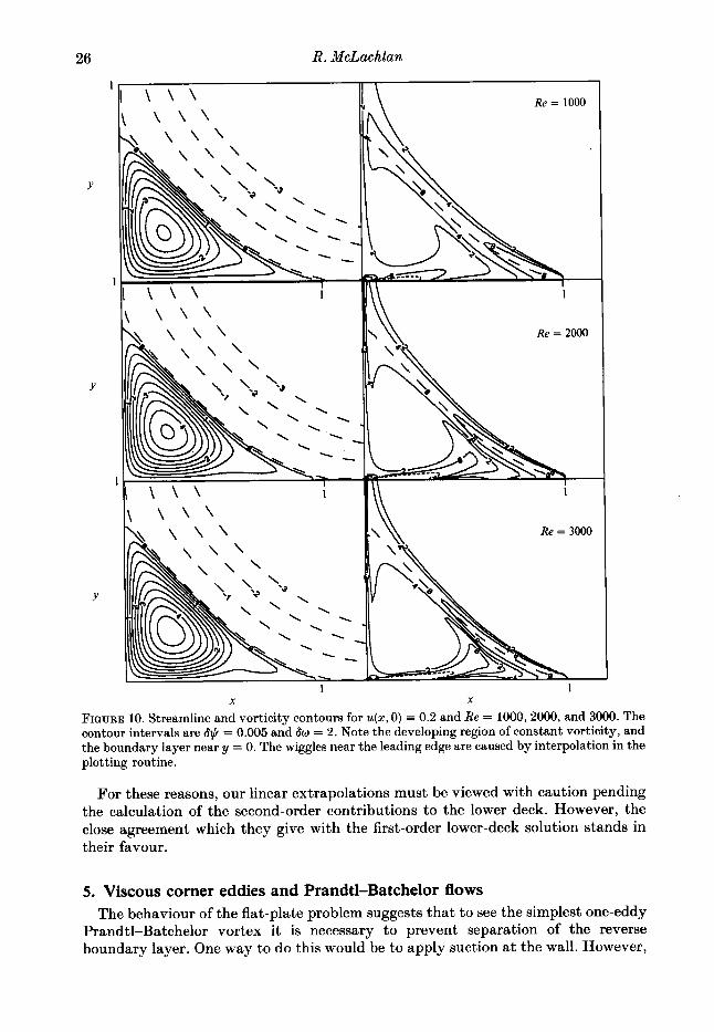
FIGURE 10. Streamline and vorticity contours for u(z,O) = 0.2 and Re = 1000,2000, and 3000. The contour intervals are &$ = 0.005 and So = 2. Note the developing region of constant vorticity, and the boundary layer near y = 0. The wiggles near the leading edge are caused by interpolation in the plotting routine.

For these reasons, our linear extrapolations must be viewed with caution pending the calculation of the second-order contributions to the lower deck. However, the close agreement which they give with the first-order lower-deck solution stands in their favour.

5. Viscous corner eddies and Prandtl-Batchelor flows The behaviour of the flat-plate problem suggests that to see the simplest one-eddy

Prandtl-Batchelor vortex it is necessary to prevent separation of the reverse boundary layer. One way to do this would be to apply suction a t the wall. However,

A steady separated viscous corner $ow (a)

27

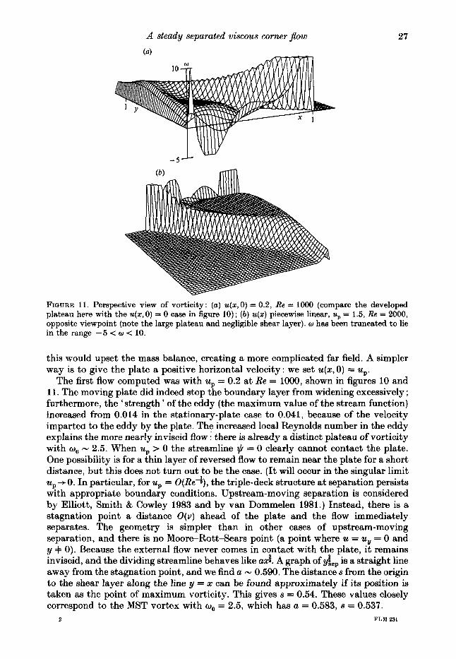
FIGURE 11. Perspective view of vorticity: (a) u(s,O) = 0.2, Re = lo00 (compare the developed plateau here with the u(z, 0) = 0 case in figure 10) ; ( b ) u(z) piecewise linear, up = 1.5, Re = 2000, opposite viewpoint (note the large plateau and negligible shear layer). o has been truncated to lie in the range -5 < w < 10.

this would upset the mass balance, creating a more complicated far field. A simpler way is to give the plate a positive horizontal velocity : we set u ( x , 0) = up.

The first flow computed was with up = 0.2 at Re = 1000, shown in figures 10 and 11. The moving plate did indeed stop the boundary layer from widening excessively ; furthermore, the ‘strength ’ of the eddy (the maximum value of the stream function) inoreased from 0.014 in the stationary-plate case to 0.041, because of the velocity imparted to the eddy by the plate. The increased local Reynolds number in the eddy explains the more nearly inviscid flow : there is already a distinct plateau of vorticity with wo - 2.5. When up > 0 the streamline $ = 0 clearly cannot contact the plate. One possibility is for a thin layer of reversed flow to remain near the plate for a short distance, but this does not turn out to be the case. (It will occur in the singular limit up + O . In particular, for up = O(Re-)), the triple-deck structure at separation persists with appropriate boundary conditions. Upstream-moving separation is considered by Elliott, Smith & Cowley 1983 and by van Dommelen 1981.) Instead, there is a stagnation point a distance O(v) ahead of the plate and the flow immediately separates. The geometry is simpler than in other cases of upstream-moving separation, and there is no Moore-Rott-Sears point (a point where u = uy = 0 and y + 0). Because the external flow never comes in contact with the plate, it remains inviscid, and the dividing streamline behaves like a d . A graph of yiep is a straight line away from the stagnation point, and we find a - 0.590. The distance s from the origin to the shear layer along the line y = x can be found approximately if its position is taken as the point of maximum vorticity. This gives s = 0.54. These values closely correspond to the MST vortex with wo = 2.5, which has a = 0.583, s = 0.537.

2 FLM 231

28 R . McLachlan

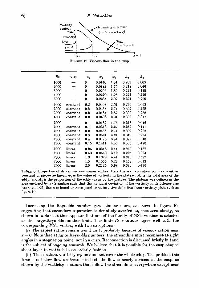
fi = 0, y - a(1 -xp

laver I \ \ y - y * :/I I-

I I

Xlelt *right x = l

FIQURE 12. Viscous flow in the cusp.

Re u ( 4 up $c wo A, A , 1000 - 0 0.0140 1.61 0.203 0.005 2000 - 0 0.0182 1.75 0.218 0.046 3000 - 0 0.0205 1.89 0.221 0.145 4000 - 0 0.0220 1.98 0.221 0.226 5000 - 0 0.0234 2.07 0.221 0.260

1000 constant 0.2 0.0408 2.51 0.296 0.068 2000 constant 0.2 0.0458 2.74 0.302 0.222 3000 constant 0.2 0.0484 2.87 0.302 0.288 4000 constant 0.2 0.0498 2.94 0.303 0.317

2000 0 0.0182 1.75 0.218 0.046 2000 constant 0.1 0.0313 2.27 0.262 0.141 2000 constant 0.2 0.0458 2.74 0.302 0.222 2000 constant 0.3 0.0621 3.21 0.340 0.294 2000 constant 0.4 0.0776 3.51 0.379 0.346 2000 constant 0.75 0.1414 4.53 0.506 0.476

2000 linear 0.25 0.0346 2.44 0.252 0.187 2000 linear 0.50 0.0550 3.19 0.295 0.324 2000 linear 1.0 0.1028 4.41 0.376 0.527 2000 linear 1.5 0.1555 5.26 0.458 0.613 2000 linear 2.0 0.2125 5.98 0.540 0.430

TABLE 6. Properties of driven viscous corner eddies. Here the wall condition on u(z) is either constant or piecewise linear, wo is the value of vorticity in the plateau, A, is the total area of the eddy, and A, is the proportion of the eddy taken by the plateau. The plateau was defined as the area enclosed by a streamline such that the standard deviation of the vorticity in its interior was less than 0.05; this was found to correspond to an intuitive definition from vorticity plots such aa figure 10.

Increasing the Reynolds number gave similar flows, as shown in figure 10, suggesting that secondary separation is definitely averted. wo increased slowly, as shown in table 6. It thus appears that one of the family of MST vortices is selected as the large-Reynolds-number limit. The finite-Re solutions agree well with the corresponding MST vortex, with two exceptions :

(i) The aspect ratios remain less than 1, probably because of viscous action near x = 0. Note that at finite Reynolds numbers, the streamline must reconnect at right angles in a stagnation point, not in a cusp. Reconnection is discussed briefly in sand is the subject of ongoing research. We believe that it is possible for the cusp-shaped shear layer to reattach in an orderly fashion.

(ii) The constant-vorticity region does not cover the whole eddy. The problem this time is not slow flow upstream - in fact, the flow is nearly inviscid in the cusp, as shown by the vorticity contours that follow the streamlines everywhere except near

A steady separated viscous corner $ow 29

Re 1 -zlert Ratio 1-zIigh, Ratio A&-: 1000 0.609 0.362 2000 0.553 0.908 0.337 0.931 0.891 3000 0.531 0.960 0.311 0.923 0.935

TABLE 7. Turning points of w = 2 contour: ‘ratio’ is the distance at that value of Re divided by the distance at the next smallest Re; the distances are predicted to go like Re-r.

the wall. Instead, disturbances generated in the downstream boundary layer are swept away from the wall by the natural motion of the eddy.

This effect can be estimated as follows. Consider the Batchelor flow with internal vorticity w . The equation for the stream function in the cusp is approximately Ic.,, = -w, with @ = 0 at y = 0 and at y = ysep = ax:, so

II. = + Y ( Y s e p - ~ ) . (5.1)

Thus the streamlines turn around (see figure 12) when u = 0, or

x = (SY, measuring distance from the leading edge. Now suppose that viscous effects do not greatly alter the flow field. Downstream, in the boundary layer, $ = u9 y+O(y2) and y = O(Red) . So streamlines (or, equivalently, vorticity contours) originating in the boundary layer will turn around when x = O(Re-i) ; the constant-vorticity region will enter the cusp very slowly. Table 7 shows that u = 0 when x = O(Re-0.135), in close agreement with the above description.

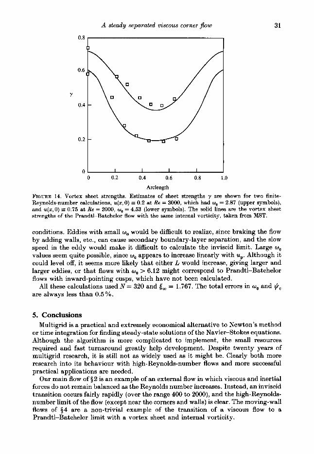
By altering the boundary condition on the plate, different members of the family of MST vortices can be found. The first set of solutions was found by setting u = up and increasing up at Re = 2000. Solutions could be found up to up = 0.85 and are shown in figure 13 (a). The flows behaved roughly like the MST family, with the eddy bulging out as wo increased, but because of the large velocity enforced near x = 1 - not present in a Prandtl-Batchelor flow - the correspondence of eddy shapes is not exact. However, the sheet strength was estimated in two cases and is shown in figure 14. The numerical values disagree by about lo%, but the broad features are correct, including a weak sheet with a boundary layer at the cusp when wo is large.

To see if fmite-Reynolds-number eddies could be found that corresponded even more closely to Prandtl-Batchelor flows, the (somewhat artificial) boundary condition was chosen in which u(x, 0) is piecewise linear, and u(0) = u(1) = 0, .(a) =

up. The lengthscale L of the corresponding Prandtl-Batchelor flow was estimated by extrapolating the y - x; behaviour to the x-axis. The dividing streamlines for six up values are shown against the position of the vortex sheet in figure 13(b) . Considering that the width of the shear layer in these cases is more than 0.1, the agreement is extremely good, and it must be concluded that for this geometry, the limit of small viscosity is indeed a Prandtl-Batchelor flow.

The results for different wall conditions are summarized in table 6. Both the internal vorticity and the relative size of the plateau region increase roughly linearly with up, the latter confirming that the presence of inviscid dynamics is controlled by the local Reynolds number.

The question arises as to whether all of the MST vortices are possible large- Reynolds-number limits of Navier-Stokes solutions with appropriate boundary

2-2

30

Y

R. McLachlan

0 0.1 0.2 0.3 0.4 0.5 0.6 0.7 0.8 0.9 1.0 1.1 X

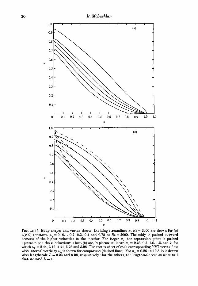
FIQURE 13. Eddy shapes and vortex sheets. Dividing streamlines at Re = 2000 are shown for (a) u(x,O) constant, up = 0, 0.1, 0.2, 0.3, 0.4 and 0.75 a t Re = 2000. The eddy is pushed outward because of the h i g F velocities in the interior. For larger up, the separation point is pushed upstream and the d behaviour is lost. (b) u(s,O) piecewise linear, u, = 0.25, 0.5, 1.0, 1.5, and 2, for which wo = 2.44, 3.19,4.41,5.26 and 5.98. The vortex sheet of each corresponding MST vortex flow with internal vorticity wo is shown for comparison (dashed lines). For up = 0.25 and 0.5, it is drawn with lengthscale L = 0.93 and 0.96, respectively; for the others, the lengthscale was so close to 1 that we used L = 1 .

A steady separated viscous corner $ow

o.8 3 31

I 1 I I

0 0.2 0.4 0.6 0.8 1 .O

Arclength

FIQURE 14. Vortex sheet strengths. Estimates of sheet strengths y are shown for two finite- Reynolds-number calculations, u(r, 0) = 0.2 a t Re = 3000, which had wo = 2.87 (upper symbols), and u(r,O) = 0.75 at Re = 2000, wo = 4.53 (lower symbols). The solid lines are the vortex sheet strengths of the Prandtl-Batchelor flow with the same internal vorticity, taken from MST.

conditions. Eddies with small uo would be difficult to realize, since braking the flow by adding walls, etc., can cause secondary boundary-layer separation, and the slow speed in the eddy would make it difficult to calculate the inviscid limit. Large oo values seem quite possible, since wo appears to increase linearly with up. Although it could level off, it seems more likely that either L would increase, giving larger and larger eddies, or that flows with wo > 6.12 might correspond to Prandtl-Batchelor flows with inward-pointing cusps, which have not been calculated.

All these calculations used N = 320 and 6, = 1.767. The total errors in wo and @c

are always less than 0.5 YO.

5. Conclusions Multigrid is a practical and extremely economical alternative to Newton’s method

or time integration for finding steady-state solutions of the Navier-Stokes equations. Although the algorithm is more complicated to implement, the small resources required and fast turnaround greatly help development. Despite twenty years of multigrid research, it is still not as widely used as it might be. Clearly both more research into its behaviour with high-Reynolds-number flows and more successful practical applications are needed.

Our main flow of $2 is an example of an external flow in which viscous and inertial forces do not remain balanced as the Reynolds number increases. Instead, an inviscid transition occurs fairly rapidly (over the range 400 to ZOOO), and the high-Reynolds- number limit of the flow (except near the corners and walls) is clear. The moving-wall flows of $4 are a non-trivial example of the transition of a viscous flow to a Prandtl-Batchelor limit with a vortex sheet and internal vorticity.

32 R. McLachlan

Although the geometry could be realized experimentally, in practice the flow would undergo a bifurcation (at a Reynolds number less than those we have considered) in which symmetry about the y-axis is lost. Nevertheless, it is essential to consider such ' artificial ' problems to get clear results, valid beyond this particular example, about high-Reynolds-number flows. For example, placing a wall at x = 0, - 00 < y < m, might be considered a more practical flow. But the extra wall brakes the eddy and the inviscid transition is not seen clearly at accessible Reynolds numbers. In addition, nested secondary eddies (as seen in the driven cavity) and Moffatt vortices complicate the corner region.

The specially chosen geometry is largely responsible for our success in confirming the Sychev triple-deck model of laminar separation. There remain questions about the effects of the complicated downstream flow, but they are most likely to be felt outside the relatively small interaction region.

This work could not have been completed without the help of my thesis advisor, H. B. Keller. I would also like to thank P. G. Saffman, for discussions on the physical basis of triple-deck theory ; D. W. Moore, for suggesting the corner flow as worthy of study, to which I owe any positive results; S. J. Cowley, for suggesting the integral test of $2.4; E. F. van de Velde, for providing me with his clearly coded multigrid Poisson solver (Velde & Keller 1987) ; and the referees for aiding the presentation. This work was supported in part by contracts DOE DE-FG03-89ER25073 and ARO DAAL03-89-K-0014, and by a New Zealand University Grants Committee Scholarship.

Addendum After this paper was completed, the work of Suh & Liu (1990) appeared. They

study the flow with walls at x = 0, - m < y < co and y = 0, 0 < x < 1. They take $ + - 2xy, so their Reynolds number Re,, is half our Re. Taking this into account, we agree with their asymptotic distance to separation in the case of a stagnant vortex (a special case of our (3.6)). But their equation (17) (used in their (18) and figure 10) gives the interaction lengthscale as Re-, whereas the correct behaviour is x -xSep - Re-:, due to Sychev (1979). We agree with their lower-Reynolds-number results, but their discretization errors appear to grow to up to 20% (in, for example, the maximum pressure gradient) at Re,, = 1600.

We disagree with their conclusion that the flow will tend to that given by the free- streamline model. Such a conclusion must be based on insufficient resolution and (local) Reynolds numbers too low to see the inviscid transition. We find no evidence of decreasing eddy velocities in any similar flow.

R E F E R E N C E S

BATCHELOR, G. K. 1956 A proposal concerning laminar wakes behind bluff bodies at large

BATCHELOR, G. K. 1967 A n Introduction to Fluid Mechanics. Cambridge University Press. BRANDT, A. 1984 Multigrid methods: 1984 Guide with Applications to Fluid Dynamics. Rehovot,

BRODETSKY, S. 1923 Discontinuous fluid motion past circular and elliptic cylinders. Proc. R. SOC.

CARPENTER, M. t HOMSY, G. M. 1990 High Marangoni number convection in a square cavity:

Reynolds number. J . Fluid Mech. 1, 38CF398.

Israel : Weizmann Institute of Science.

L d . A 102, 542-553.

Part 11. Phys. Fluids A 2 , 137-149.

A steady separated viscous corner flow 33

CARRIER, G. F. & LIN, C. C. 1948 On the nature of the boundary layer near the leading edge of a flat plate. Q. Appl. Maths 6 , 63-68.

CHENG, H. K. 1984 Laminar separation from airfoil beyond trailing edge stall. AIAA Paper 84- 1612.

CHENG, J. K. & LEE, C. J. 1985 Laminar separation studied as an airfoil problem. In Proc. Symp. Numer. Phys. Aspects Aerodyn. Flouls III (ed. T. Cebeci). Springer.

CHENG, J. K. & SMITH, F. T. 1982 The influence of airfoil thickness and Reynolds number on separation. J. Appl. Math. Phys. 33, 151-180.

DANIELS, P. G. 1979 Laminar boundary layer reattachment in supersonic flow. J. Fluid Mech. 90, 289-303.

DENNIS, S.C. R. & SMITH, F.T. 1980 Steady flow through a channel with a symmetrical constriction in the form of a step. Proc. R . SOC. Lond. A 372, 393414.

DOMMELEN, L. L. VAN 6 SHEN, S. F. 1984 Interactive separation from a fixed wall. In Proc. Symp. Numer. Phys. Aspects Aerdyn. Flows, 2nd Long Beach Conf. (ed. T. Cebeci), Springer.

ELLIOTT, J. W., SMITH, F. T. & COWLEY, S. J. 1983 Breakdown of boundary layers: (i) on moving surfaces ; (ii) in semi-similar unsteady flow; (iii) in fully unsteady flow. Geophys. Astrophys. Fluid Dyn. 25, 77-138.

FORNBERG, B. 1980 A numerical study of steady viscous flow past a circular cylinder. J. Fluid Mech. 98, 81S855.

FORNBERG, B. 1985 Steady viscous flow past a circular cylinder up to Reynolds number 600. J . Comput. Phys. 61, 297-320.

KOROLEV, C. P. 1980 TsAGI, Uch. Zpp, 11, 7-16. LEAL, L. G. 1973 Steady separated flow in a linearly decelerated free stream. J . Fluid Mech. 59,

MCLACHLAN, R. I. 1990 Separated viscous corner flows via multigrid. Ph.D. thesis, California

MCLACHLAN, R. I. 1991 The boundary layer on a finite flat plate. Phys. Fluids A 3, 341-348. MESSITER, A. F. 1975 Laminar separation - a local asymptotic flow description for constant

pressure downstream. AGARD Symp. on Separated Flows. MILOS, F. S., ACRIVOS, A. & KIM, J. 1987 Steady flow past sudden expansions a t large Reynolds

number 11. NavierStokes solutions for the cascade expansion. Phys. Fluids 30, 7-18. MOORE, D. W., SAFFMAN, P. G. 6 TANVEER, S. 1988 The calculation of some Batchelor flows: the

Sadovskii vortex and rotational corner flow. Phys. Fluids 31, 978-990 (referred to herein as MST) .

PEPIN, F. M. 1990 Simulation of the flow past an impulsively started cylinder using a discrete vortex method. Ph.D. thesis, GALCIT, California Institute of Technology.

PRANDTL, L. 1905 Motion of fluids with very little viscosity. Gottingen; transl. in NACA TM-452 (1928).

SCHREIBER, J. & KELLER, H. B. 1983 Driven cavity flows by efficient numerical techniques. J. Comput. Phys. 49, 310-333.

SMITH, F. T. 1977 The laminar separation of an incompressible fluid streaming past a smooth surface. Proc. R . SOC. Lond. A 356, 443-463.

SMITH, F. T. 1979 Laminar flow of an incompressible fluid past a bluff body: the separation, reattachment, eddy properties and drag. J. Fluid Mech. 92, 17 1-205.

SMITH, F. T. 1981 Comparisons and comments concerning recent calculations for flow past a circular cylinder. J. Fluid Mech. 113, 407410.

SMITH, F. T. 1986 Steady and unsteady boundary-layer separation. Ann. Rev. Fluid Mech. 18,

SMITH, F. T. 1987 Theory of high-Reynolds-number flow past a blunt body. In Studies of Vortex

SMITH, J. H. B. 1982 The representation of planar separated flow by regions of uniform vorticity.

SMITH, J. H. B. 1986 Vortex flows in aerodynamics. Ann. Rev. Fluid Mech. 18, 221-242.

513-535.

Institute of Technology.

197-220.

Dominated Flows (ed. M. Y. Hussaini & X. Salas). Springer.

In Vortex Motion, pp. 157-172. Vieweg.

34 R. McLachlan

STEWARTSON, K. 1974 Multistructured boundary layers on flat plates and related bodies. Adv. Appl. Mech. 14, 145.

SUH, Y. K. & LIU, C. S. 1990 Study on the flow structure around a flat plate in a stagnation flow field. J. Fluid Mech. 214, 489487.

SYCHEV, V. V. 1972 Concerning laminar separation. Izv. Akad. Nauk. SSSR, Mekh. Zhid. Gaza 3 , 47-59.

SYCHEV, V. V. 1979 Boundary layer separation from a plane surface. TsAGI, Uch. Zap. 9,20-29; (transl. in NASA TM-75828).

VELDE, E. F. VAN DE & KELLER, H. B. 1987 The parallel solution of nonlinear elliptic equations. In Parallel Computations and Their Impact ME Mechanics (ed. A. K. Noor), pp. 127-153.

WOODS, L. C. 1954 Aeronaut. Q. 5, 176-184.