A Step towards Automated Design of Side Actions in Injection Molding of Complex Parts

Ashis Gopal Banerjee1 and Satyandra K. Gupta2

1,2Department of Mechanical Engineering and The Institute for Systems Research

University of Maryland College Park, MD 20742, USA

1ashis@umd.edu2skgupta@eng.umd.edu

Abstract. Side actions contribute to mold cost by resulting in an additional manufacturing

and assembly cost as well as by increasing the molding cycle time. Therefore, generating shapes of side actions requires solving a complex geometric optimization problem. Different objective functions may be needed depending upon different molding scenarios (e.g., prototyping versus large production runs). Manually designing side actions is a challenging task and requires considerable expertise. Automated design of side actions will significantly reduce mold design lead times. This paper describes algorithms for generating shapes of side actions to minimize a customizable molding cost function.

1 Introduction

Injection molding is one of the most widely used plastic manufacturing processes nowadays [1]. It is a near net-shape manufacturing process that can produce parts having good surface quality and accuracy. Moreover, this process is suitable for mass volume production due to fast cycle time. Often complex injection molded parts include undercuts, patches on the part boundaries that are not accessible along the main mold opening directions. Undercuts are molded by incorporating side actions in the molds. Side actions are secondary mold pieces (core and cavity form the two main mold pieces) that are removed from the part using translation directions that are different from the main mold opening direction (also referred as parting direction). Use of side actions is illustrated in Fig. 1.

Significant progress has been made in the field of automated mold design. Chen et al [2] linked demoldability (i.e. the problem of ejecting all the mold pieces from the mold assembly such that they do not collide with each other and with the molded part) to a problem of partial and complete visibility as well as global and local interference. If a surface is not completely visible, then either it is blocked locally by parts of the same surface, or globally by other surfaces. They reduced global accessibility of undercuts (or pockets that are the non-convex regions of a part) to a local problem and used visibility maps. Hui [3] classified undercuts into external and internal, which require side and split cores for removing them from the main mold pieces respectively. He primarily focused on obtaining optimal parting directions from a set of heuristically generated candidate directions by minimizing the number of such side and split cores. Since then, Yin et al [4] have tried to recognize undercut features for near net-shape manufactured parts by using local freedom of sub-assemblies in

2

directed blocking graphs. Another way of recognizing and especially categorizing undercuts was put forward by Fu et al. [1]. A ray tracing/intersection method for finding out release directions in injection-molded components was suggested by Lu et al. [5]. Chen and Rosen [6] suggested partitioning part faces into regions, consisting of generalized pockets and convex faces, each of which can be formed by a single mold piece.

Mold piece touching facets on this hole cannot be moved in + d or – d. Facets in the hole are undercut

facets

- d

Main mold opening

directions

Side action

Removal direction of side action is different

from + d or - d

Part + d

Fig. 1. Side action to remove the undercut facets in a direction different from the main mold opening direction

Dhaliwal et al. [7] described exact algorithms for computing global accessibility

cones for each face of a polyhedral object. Using these, Priyadarshi and Gupta [8] developed algorithms to design multi-piece molds. Ahn et al. [9] have given theoretically sound algorithms to test whether a part is castable along a given direction in O(n log n) time and compute all such possible directions in O(n4) time. Building on this, Elber et al. [10] have developed an algorithm based on aspect graphs to solve the two-piece mold separability problem for general free-form shapes, represented by NURBS surfaces. Recently, researchers [11, 12] have presented new programmable graphics hardware accelerated algorithms to test the moldability of parts and help in redesigning them by identifying and graphically displaying all the mold regions (including undercuts) and insufficient draft angles.

Due to space restrictions, it is difficult to present a detailed review of all the other work in the mold design area. So, we will identify some of the important work in this field. Representative work in parting surface and parting line design includes [13] and [14] respectively. Representative work in the area of undercut feature recognition was done by [15], whereas same in the area of side core design includes [16].

Thus, we can summarize that the problem of finding optimum parting direction has been studied extensively and is very useful in casting applications. However, in case of injection molded plastic parts, most designers develop part designs with a mold opening direction in mind. This is because mold opening direction influences all aspects of part design. Typically, plastic parts are either flat or hollow-box shaped and they need to have relatively thin sections. These shapes have an implied mold opening direction. Moreover, they cannot have vertical walls; and some amount of taper has to

3

be imparted to them in order to remove them from the mold assembly. Therefore the main tasks in injection mold design automation are (1) determination of the main parting line and parting surface, (2) recognition of undercuts, and (3) design of side actions. Existing methods for the first two tasks provide satisfactory solutions.

However, existing techniques for side action design do not work satisfactorily if a complex undercut region (1) needs to be partitioned to generate side actions, or (2) has finite accessibility. Fig. 2 shows two parts for which generating side actions is challenging due to these two reasons. In this paper, we present a new algorithm to handle these types of cases. We currently only consider those types of side actions that are retracted from the undercut in a direction perpendicular to the main mold opening direction. In fact, majority of side actions used in industrial parts meet this restriction. Typically, a single side action produces a connected undercut region. Therefore, we treat each connected undercut independently and generate appropriate number of side actions for molding it.

Fig. 2. Parts that pose challenges for existing side action design algorithms

Undercut has finite accessibility

(b)

Connected undercut region needs partitioning

(a)

2 Problem Formulation and Theoretical Foundations

Retraction is defined by a point (x, y) in R2. We are interested in two types of retractions namely, core-retractions and cavity-retractions.

Retraction length is defined as the length of the position vector of the 2D point that defines the corresponding retraction.

A given retraction (x, y) is a feasible core retraction for an undercut facet f, if

sweeping f first by a translation vector and then by another one t l , (where is a large positive number) does not result in any intersection with the part. Fig. 3 shows examples of a feasible and an infeasible core retraction.

^ ^

1t x i y→

= + j k→

=

i y j→

= + l k→

= −

^

2 a

al

A given retraction (x, y) is a feasible cavity retraction for an undercut facet f, if

sweeping f first by a translation vector t x and then by another one t , does not result in any intersection with the part.

^ ^

1

^

2 a

4

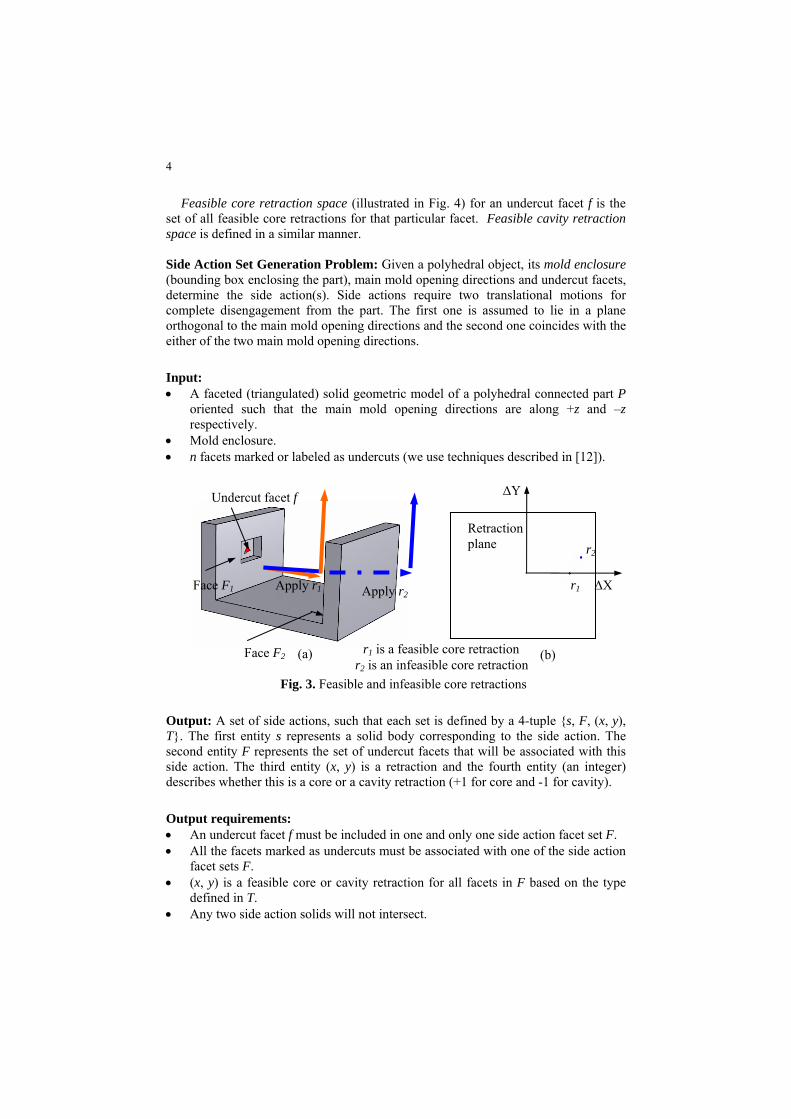
Feasible core retraction space (illustrated in Fig. 4) for an undercut facet f is the set of all feasible core retractions for that particular facet. Feasible cavity retraction space is defined in a similar manner.

Side Action Set Generation Problem: Given a polyhedral object, its mold enclosure (bounding box enclosing the part), main mold opening directions and undercut facets, determine the side action(s). Side actions require two translational motions for complete disengagement from the part. The first one is assumed to lie in a plane orthogonal to the main mold opening directions and the second one coincides with the either of the two main mold opening directions.

Input: • A faceted (triangulated) solid geometric model of a polyhedral connected part P

oriented such that the main mold opening directions are along +z and –z respectively.

• Mold enclosure. • n facets marked or labeled as undercuts (we use techniques described in [12]).

Fig. 3. Feasible and infeasible core retractions

(a)

Apply r2Apply r1Face F1

Face F2

ΔX

(b)

Retraction plane

r1 is a feasible core retraction

r1

r2

r2 is an infeasible core retraction

ΔY Undercut facet f

Output: A set of side actions, such that each set is defined by a 4-tuple {s, F, (x, y), T}. The first entity s represents a solid body corresponding to the side action. The second entity F represents the set of undercut facets that will be associated with this side action. The third entity (x, y) is a retraction and the fourth entity (an integer) describes whether this is a core or a cavity retraction (+1 for core and -1 for cavity).

Output requirements: • An undercut facet f must be included in one and only one side action facet set F. • All the facets marked as undercuts must be associated with one of the side action

facet sets F. • (x, y) is a feasible core or cavity retraction for all facets in F based on the type

defined in T. • Any two side action solids will not intersect.

5

• The side actions generated will minimize the following objective (molding cost) function:

^ ^ ^ ^/

1 1

kN N

i i i ii i

C x i y j NC x i y jγ χ= =

= + + + +∑ ∑ (1)

where is the cardinality of the output set, N ( ),i ix y is the retraction in the ith

element of the set, and γ , , , k /C χ are molding parameters. Here γ is a proportionality constant that relates the machining cost to the complexity of the solid shape, is an exponent (obtained experimentally) associating shape complexity with the retraction length, is the cost of actuating and assembling side action associated with core or cavity-retraction and

k/C

χ relates retraction length to the cost incurred due to increase in molding cycle time. It is important to note that depending on the geographical region and the nature of the molding operation, values of these parameters will be significantly different for the same part. In other words, these parameters might have altogether different values for production-run molds and prototyping molds even for the same part.

Maximum error is equal to half the greatest length possible for any cell edge

ΔX

ΔY

Retraction plane

Boundary due to face F1

Feasible retraction space

Boundary due to face F2

Fig. 4. Feasible core retraction space Fig. 5. Maximum error in retraction length

For each undercut facet we will compute its feasible retraction space (see Section 3 for details on this step) that can be represented as a set of one or more disjoint polygons in 2D translation space (ΔXY plane). This translation space can be bounded on all the four sides by the mold enclosure and is termed as the retraction plane. Eventually, we get a set of feasible retraction spaces on the retraction plane. The objective function for this problem calls for minimizing the number of side actions as

Optimum retraction

Cell

ΔX

ΔY

Boundary due to the other faces (side walls) of the undercut

Retraction returned by our algorithm Boundary so that feasible retraction comprises of a

single horizontal translation vector along with another vertical translation vector

6

well as the retraction lengths. Therefore, usually a compromise needs to be worked out by identifying a suitable set of feasible retractions.

The set of feasible retraction spaces can be partitioned into a set of cells and let A to be the spatial (planar) arrangement defined by them. This arrangement A is computed by intersecting and splitting the feasible retraction spaces for all the facets. Hence, for each cell a in A, the set of undercut facets for which this cell will be a subset of its corresponding feasible retraction space is known. This set of facets is termed as the retractable facets for the cell a. In other words, all retractions defined by points located within a are feasible for all the retractable facets. Since by selecting such a retraction, we will be able to deal with a large number of retractable facets at one go, we will then perform a search over all cells and find the optimal combination of retractions.

Although, we follow the described methodology in spirit, an attempt to explicitly generate A leads to implementation challenges due to robustness problems. Hence, we focus on finding a discrete set of promising retractions and performing search over them. In the following sections, we explain our methodology to do the same. But before we proceed, let us establish some important foundations and properties.

Lemma 1: Let r be a retraction used in the optimal solution and F be the set of

facets associated with r. Then r will lie on the boundary of a cell in A. Proof: Since we are minimizing the objective (molding cost) function, if retraction

r belongs to the optimal solution, then the corresponding retraction length must have the least possible value. Since the associated facet set F corresponds to a particular cell in A, r must lie on the boundary of that cell, as the point having minimum distance from the origin (i.e. retraction length) for any polygonal cell will be a boundary point. Hence the assertion of lemma directly follows from this observation.

This lemma clearly points out that we only need to consider the boundary of the

cells in A and hence the interior of the cells can be safely ignored. Now let us consider a set R that consists of two types of elements - the original corner vertices of all the feasible retraction space polygons and the intersection points obtained by pair-wise intersection of all edges in the feasible retraction space polygons. This set R includes all the vertices of the arrangement A.

Lemma 2: Let F be a facet group in the optimal solution. Then there will exist a

retraction r in R such that r is a feasible retraction for all facets in F. Proof: Since F is a facet group present in the optimal solution, if retraction r is a

feasible retraction for all facets in F, then it must be contained (either on the boundary or within the interior) in the particular cell corresponding to F (see Lemma 1).

Now, the set of retractable facets corresponding to a particular cell does not change within its interior. It definitely changes at the 0-faces, i.e. at the original corner vertices of the free space polygons or at the intersection points. The status of the edges is rather hard to determine. While the boundary edges (edges belonging to a single cell only) have the same set of facets as the respective cell interiors, edges that are common to multiple cells have an ambiguous status. However, this is immaterial here since any change in the retractable facet set along an edge is already accounted

7

by the two vertices forming the edge. Since the set R encompasses all the 0-faces of the cells, r is bound to be present in R and thus, the lemma follows.

Based on Lemma 2, we can utilize R as our search space instead of actually

computing A. However, if the solution actually lies on the edge of a cell, we might not get the optimal solution. In order to minimize this error, we facet the edges of the feasible retraction space polygons a priori (before computing the line segment intersections) so that no two neighboring vertices are more than ε apart from each other on any of the sides. Still the retraction lengths in our solution might be marginally greater than or equal to the optimum retraction lengths. However, Theorem 1 formalizes that such an error will be bounded.

Theorem 1: Let S* be the optimal solution and let S’ be a solution that has the

same facet sets but each retraction length is increased by 0.5ε . Then the solution produced by our algorithm will be no worse than S’.

Proof: As Fig. 5 points out, maximum error in retraction length occurs when the optimum solution lies at the mid-point of an edge and the solution explored by our algorithm by searching over the set R, corresponding to the same facet set is obviously one of the edge vertices. If the optimum retraction corresponds to any other point on the edge, then the closer neighboring vertex will be considered by our algorithm. There are two possibilities. First, our algorithm will return this solution, resulting in a small error. This difference is, of course, bounded by half the maximum possible edge length, i.e. by 0.5 ε . Second, our algorithm will find a better solution than this one.

From the above argument, it easily follows that since solution S/ has identical facet sets as the optimum solution S*, but each retraction length is increased by 0.5ε , our algorithm will not generate solution worse than S/.

Choosing ε to be equal to 1 mm, there is very little qualitative difference between

the solution generated by our algorithm and the optimum one. Practically this error has no effect, since a discrepancy of 0.5mm in the retraction length hardly matters due to use of fast actuators attached to side actions. Thus, this error is insignificant.

3 Constructing Feasible Retraction Space

From the discussion in the previous section, it is clear that we first need to construct the feasible retraction space for every individual undercut facet. This is done in two stages. Initially, a feasible space needs to be computed on the retraction plane such that a single horizontal translation vector can pull the facet there without being obstructed by any other facet lying on the way. So, all the potential facets capable of causing obstruction need to be identified. Since the translation vector in our case is restricted to lie in a horizontal plane, it makes sense to consider all the facets lying partially or completely within the z-range of the undercut facet under consideration as potential obstacles. Z-range refers to the 3D space bounded by the maximum and the minimum z coordinate values of the facet vertices. In case a facet does not lie

8

completely within the z-range, only the part of it lying inside is considered. This involves truncation of triangular facets to form convex polygons of 3, 4 or 5 sides.

According to Aronov and Sharir [17], 3D free configuration space FP of a convex “robot” B moving in space occupied by k/ obstacles {A1, …, Ak

/} is given as the

complement C of U, where be the union of the so-called expanded

obstacles P

/

1

k

ii

U=

=UP

i. Here Pi is the Minkowski sum of Ai and – B, for i = 1,…, k/. Collision polyhedron for a facet f with respect to another facet f/ is defined as the

set of points in 3D translation space such that if corresponding translations are applied to f, then the translated f intersects with f/.

Collision polygon for a facet f with respect to another facet f/ is defined as the set of points in 2D translation space such that if corresponding translations are applied to f, then the translated f intersects with f/.

In this case, replacing B by the undercut facet under consideration and Ais by the k/

facets falling within its z-range, set of collision polyhedrons are obtained. This Minkowski sum is computed easily by obtaining the convex hull of the vector differences of each pair of vertices,. The collision polyhedrons are then intersected by a horizontal plane located at Δ z = 0 to obtain collision polygons in the retraction plane. However, the fact that the facet must be able to reach this feasible space by means of a single translation vector also needs to be taken into account here. That is why, mere construction of Minkowski polyhedrons and then intersection with a horizontal plane do not give the final obstructed space.

Sweep-based collision polygon for a facet f with respect to another facet f/ is defined as the set of points in 2D translation space such that if corresponding

translations are applied to f, the swept polygon P will intersect ft→

/, where

. }10,:{ ≤≤∈+=→

ξξ fptpPCollision free 2D translation space for a facet f is defined as the set of points in 2D

translation space such that if corresponding translations are applied to f, the swept polygon P (defined as before) will not intersect with any of the collision facets f

t→

/. The hard shadows of all the k/ collision polygons need to be computed in order to

determine the sweep-based collision polygons. Alternatively, same thing is done by plane sweeping the collision polygons until they reach the retraction plane boundaries. Lastly, the collision free 2D translation space is obtained by subtracting the union of the forbidden spaces from the bounded retraction plane. The steps are schematically shown in Fig. 6.

In order to ensure that the horizontally translated undercut facet can also be pulled vertically, it is necessary to construct another feasible space on the retraction plane. This transformation space is called 2D translation space for upward vertical accessibility for a facet f. It is defined as the set of points in 2D translation space such that if this translation is applied to f, then it can be released vertically upwards. Similarly, a 2D translation space for downward vertical accessibility can also be defined for facet f. This direction of possible release provides a natural way of classifying feasible retractions into feasible core retractions and feasible cavity retractions. In order to compute this space, the entire mold free space (regularized

9

Boolean difference between the mold enclosure and the part) is voxelized. Each voxel is then analyzed for vertical accessibility and a procedure similar to the previous one is adopted. Finally, the intersection of the collision-free 2D translation space and the 2D translation space for upward (or downward) vertical accessibility is taken to identify the feasible core (or cavity) retraction space for every individual undercut facet. If voxels are accessible along both +z as well as –z directions, then they are either merged with voxels accessible along +z or –z depending upon the nature of the neighboring voxels. In general we prefer feasible cavity retractions because side actions associated with cavity retractions are easier to realize in practice.

Sweep-based collision polygon (only w.r.t. f2)

Find Minkowski sum, transform to retraction plane and sweep it Part

Cross-sectional view

Find facets lying within z-range of f1f1 f2

ΔX

ΔY

Repeat these steps for all undercut facets

Collision polygon w. r. t. f2 (shown by

dotted lines)

ΔX

ΔY Undercut facet d

Compute the union and take complement

- z f1

+z

Collision-free 2D translation space (all the facets taken into account)

Main mold opening directions

Fig. 6. Constructing collision-free 2D translation space

4 Computing Discrete Set of Candidate Retractions

As discussed in Section 2, the aim is to obtain the discrete set of all possible retractions. Firstly, edge faceting is carried out on all the feasible retraction space polygons if necessary and then all the line segment intersection points are computed. The corner points of all the retraction space polygons are also retained. Next we need to prune the set of retractions to obtain a so-called non-dominated set. Such a set will only consist of those retractions which are better than any other in the entire set with respect to either the retraction length or the number of associated facets. This is done by first sorting all the retractions in order of increasing retraction lengths. Then we search for all the retractions that have identical retraction lengths and again sort them

10

in order of their number of retractable facets. We delete all the retractions that have lesser number of associated facets than the current maximum value. Initially, this current maximum is equal to zero and we keep on updating it as we progressively consider one retraction length bucket after another.

Once all the non-redundant retractions have been computed, we can start constructing a tree to represent our feasible solution space. In order to do that, we need to sort the undercut facets in a particular way, so that the process of placing the nodes gets facilitated. A heap is built for the n undercut facets where they are arranged depending upon their minimum retraction lengths (with highest preference being given to those having maximum values of minimum retraction lengths). Ties are broken on the basis of lesser number of associated retractions. This heap is used as an efficient priority queue.

Moreover, a linked list is used so that access from facets to retractions can be done easily in constant time. For a particular element in the linked list, i.e. an undercut facet, all the associated retractions are maintained in a sorted order depending upon their lengths, with highest preference being given to the one(s) having least magnitude. This is utilized while placing the actual nodes in the search tree. All these data structures are created so that queries become efficient while traversing the search tree to obtain an optimal solution to the undercut region grouping problem. They ensure that we do not need to perform more than O(n log n) computations at any node in any level of the tree, instead of the usual O(n2) calculations necessary if we carry out exhaustive comparisons and enumerations.

5 Generating Side Actions

A depth-first branch and bound algorithm is used to determine the optimal set of undercut regions. This requires us to employ intelligent heuristics to quickly steer search to a good initial solution, limit branching, and prune as many search paths as possible. The notion of a bottleneck facet plays a key role in realizing these heuristics. It may be observed that certain facets become the main bottlenecks in generating a solution. These facets have very limited number of feasible solutions and they impose constraints on the goodness of the overall solution. The overall solution has to address these facets and hence it is desirable to process them first. These facets belong to the category such that the minimum retraction length for them is maximum among all the facets. On top of this, they must have rather narrow feasible retraction spaces, which, in turn, will be reflected in the fact that they will have smaller number of retractions associated with them.

Once bottleneck facets have been identified, we will start constructing the search space with any one of them. An empty node is created as the root node and all the vertices associated with the chosen bottleneck facet (highest priority element in our heap) are placed as top level nodes in the search space. Since we will access the vertices directly using the linked list, they will be placed in order of increasing retraction lengths. If we consider a particular retraction, its associated retractable facets form the first undercut region. In the next level, we need to determine the bottleneck facets among the remaining ones and place the vertices attached to any one

11

of them as nodes. We proceed in this manner until all facets are covered. Of course, we need to be careful not to include two vertices such that the horizontal translation vectors corresponding to the retractions intersect with each other in the final solution. Such a path, if encountered, will be termed as infeasible and will be pruned. If some of the retractable facets associated with a retraction are already covered then they will not be added to this solution.

We keep track of the current best solution. If during the search, cost of a partial solution exceeds the cost of current best solution, then this path is pruned. If during the search a better solution than the current best solution is found then the current best solution is updated. Search can terminate in two ways. Firstly, it terminates when all promising nodes have been explored. In this case it produces a solution very close to the optimal solution. Secondly, it stops when the user specified time limit has been exceeded. In this case search returns the current best solution.

The bottleneck facet scheme restricts the amount of branching (or number of nodes) at a particular search level. Now coming to the tree depth issue, it is rare to find parts in which a connected undercut region requires more than three side actions. Usually cost function parameters are such that solutions involving N + 1 side actions are more expensive than a solution involving N side actions. Our heuristics enable us to quickly locate feasible solutions and once a feasible solution has been found, very few nodes are explored at the next depth level. Hence, for virtually all practical parts we should be able to find optimal solutions in a reasonable amount of time. As with any depth first branch and bound algorithm, the time complexity increases exponentially with the depth of the search tree. However, since we do not expect practical cases involving more than three side actions for a single undercut region, the exponential growth is not much of a concern in this particular application.

Once all the regions have been generated, they are swept along the associated horizontal translation vectors (corresponding to the retractions) and additional patches are included at the top, bottom and the arrow-tip end of the vector to form a compact, 2-manifold solid. These capping patches consist of planar faces only. The boundaries of these solids are then triangulated to represent them in a faceted format and they form the desired set of side actions.

6 Results

All the algorithms were implemented in C++ using Visual Studio.NET 2003 in Windows XP Professional operating system. CGAL [18] version 3.0.1 was used as the geometric kernel. In order to speed up computation, all the vertex coordinates were first converted into integral values and then the Cartesian kernel with int number type was used. CAD model for every part was triangulated and converted into .stl format which was then taken as input by the program. The main mold opening direction was inputted separately. A preprocessor program was written to recognize all undercut facets. All the programs were run in a Pentium M processor machine having 512 MB of RAM and processor clock speed of 1.6 GHz.

A series of computational experiments have been carried out on 4 parts to characterize the performance of the algorithms. Since we cannot compare time values

12

across different parts, we decided to facet each part using four different levels of accuracy. Now comparisons with respect to computation time, number of nodes in search space and so on can be made for the same part having varying number of facets. Results of these experiments for γ = 200 (in $/mm2), = 2, = 5,000 or 10,000 (in $) depending upon whether it is a cavity or core retraction, and

k /Cχ = 18.227

(in $/mm) are shown in Table 1 below. These values are based on a specific injection molding scenario. The side action solids generated for the four test parts have been displayed in Fig. 7.

Certain basic trends are discernible from the values in the table. Of course, both the feasible retraction space and candidate retraction computation times increase as we go for higher number of facets to represent the part. However, for parts A and B where the numbers of undercut facets remain same, although the overall numbers of facets increase, this trend is markedly different from parts C and D. The retraction space computation time increases linearly, whereas candidate retraction calculation time remains more or less constant in the former case. In the latter case, feasible retraction space construction time increases almost quadratically, while the retraction computation time increases at a rate slightly greater than linear, but less than quadratic, indicating possibly a linear-logarithmic growth. Overall an optimal set of 2 or 3 side actions were generated for four sample parts in about 30-50s. This is a reasonably good performance and can serve as the foundation step towards our eventual goal of fully automatic side action design.

Table 1. Results of computational experiments

Part Model Total # of

facets

# of undercut

facets

Feasible retraction

space computation time (in s)

Candidate retraction generation time (in s)

Depth-first branch and

bound computation time (in s)

# 1 224 36 3.5 2.2 27.0 # 2 256 36 4.0 2.4 28.0 # 3 336 36 4.8 2.8 30.0

A

# 4 568 36 6.1 3.3 32.0 # 1 378 122 6.0 5.2 36.0 # 2 570 122 7.4 5.5 36.0 # 3 716 122 8.5 5.7 36.5

B

# 4 882 122 10.0 5.8 37.0 # 1 414 175 5.9 6.4 2.3 # 2 478 188 6.3 6.5 2.3 # 3 576 194 7.1 6.7 2.4

C

# 4 882 249 12.2 7.6 2.5 # 1 376 60 0.3 3.5 3.2 # 2 814 122 1.0 5.9 3.3 # 3 1324 156 2.1 9.0 3.5

D

# 4 2002 218 4.4 16.3 3.9

13

A B

C D

Fig. 7. Side action solids for 4 different test parts (A, B, C, D) shown in retracted state

7 Conclusions

New algorithms to automatically generate shapes of side actions have been presented in this paper. The major contributions of our work can be summarized as follows. It is capable of designing side actions for complex undercuts that are finitely accessible. Then it successfully partitions connected undercut regions (for which no single side action exists) into smaller regions, such that each of them can be molded by separate side actions and a customizable molding cost function is minimized. Many of the steps in the computation of feasible retraction space and discrete set of candidate retractions have linear or linear-logarithmic worst-case asymptotic time complexities. Few grow quadratically with an increase in the total number of part facets as well the number of undercut facets. Finally, if a connected undercut region can be molded by 3 or fewer number of side actions, then empirical results suggest that our algorithm is capable of finding a solution very close to the optimal solution in a reasonable amount of time for most practical parts.

This paper focuses on a particular type of side action, commonly known as side core in molding terminology. Further work needs to be done to generalize our method to design other kinds of side actions, namely, split cores, lifters etc. We will also continue working on improving our edge-faceting scheme, so that we can come up with stronger theoretical results to rule out such operations for a majority of feasible retraction space polygonal edges. In addition, we plan to incorporate better forward looking cost bounding functions to prune larger number of nodes in the search tree.

14

Acknowledgements: This work has been supported by NSF grant DMI-0093142.

However, the opinions expressed here are those of the authors and do not necessarily reflect that of the sponsor. We would also like to thank the reviewers for their comments that improved the exposition.

References

[1] Fu, M. W., Fuh, J. Y. H., Nee, A. Y. C.: Undercut feature recognition in an injection mould design system. Computer Aided Design, Vol. 31, No. 12, (1999), 777-790

[2] Chen, L-L., Chou, S-Y., Woo, T. C.: Partial Visibility for Selecting a Parting Direction in Mould and Die Design. Journal of Manufacturing Systems, Vol. 14, No. 5, (1995), 319-330

[3] Hui, K. C.: Geometric aspects of the mouldability of parts. Computer Aided Design, Vol. 29, No. 3, (1997), 197-208

[4] Yin, Z. P., Ding, H., Xiong, Y. L.: Virtual prototyping of mold design: geometric mouldability analysis for near net-shape manufactured parts by feature recognition and geometric reasoning. Computer Aided Design, Vol. 33, No. 2, (2001), 137-154

[5] Lu, H. Y., Lee, W. B.: Detection of interference elements and release directions in die-cast and injection-moulded components. Proceedings of the Institution of Mechanical Engineers Part B Journal of Engineering Manufacture, Vol. 214, No. 6, (2000), 431-441

[6] Chen, Y., Rosen, D. W.: A Region Based Method to Automated Design of Multi-Piece Molds with Application to Rapid Tooling, Journal of Computing and Information Science in Engineering, Vol. 2, No. 2, (2002), 86-97

[7] Dhaliwal, S., Gupta, S. K., Huang, J., Priyadarshi, A.: Algorithms for Computing Global Accessibility Cones. Journal of Computing and Information Science in Engineering, Vol. 3, No. 3, (2003), 200-209

[8] Priyadarshi, A.K., Gupta, S. K.: Geometric algorithms for automated design of multi-piece permanent molds. Computer Aided Design, Vol. 36, No. 3, (2004), 241-260

[9] Ahn, H-K., de Berg, M., Bose, P., Cheng, S-W., Halperin, D., Matousek, J., Schwarzkopf, O.: Separating an object from its cast. Computer Aided Design, Vol. 34, No. 8, (2002), 547-559

[10] Elber, G., Chen, X., and Cohen, E.: Mold Accessibility via Gauss Map Analysis. Journal of Computing and Information Science in Engineering, Vol. 5, No. 2, (2005), 79-85

[11] Kharderkar, R., Burton G., McMains, S.: Finding Feasible Mold Parting Directions Using Graphics Hardware. In Proceedings of the 2005 ACM symposium on Solid and Physical Modeling, Cambridge, MA, (2005), 233-243

[12] Priyadarshi, A.K., Gupta, S. K.: Finding Mold-Piece Regions Using Computer Graphics Hardware. In Proceedings of Geometric Modeling and Processing, Pittsburgh, PA, (2006)

[13] Ravi, B., and Srinivasan, M. N.: Decision criteria for computer-aided parting surface design. Computer Aided Design, Vol. 22, No. 1, (1990), 11-18

[14] Wong, T., Tan, S. T., Sze, W. S.: Parting line formation by slicing a 3D CAD model. Engineering with Computers, Vol. 14, No. 4, (1998), 330-343

[15] Ye, X. G., Fuh, J. Y. H., Lee, K. S.: A hybrid method for recognition of undercut features from moulded parts. Computer Aided Design, Vol. 33, No. 14, (2001), 1023-1034

[16] Shin, K. H., Lee, K.: Design of Side Cores of Injection Mold from Automatic Detection of Interference Faces. Journal of Design and Manufacturing, Vol. 3, No. 4, (1993), 225-236

[17] Aronov, B., Sharir, M.: On Translational Motion Planning of a Convex Polyhedron in 3-Space. Siam Journal of Computing, Vol. 26, No. 6, (1997), 1785-1803

[18] Cgal.org.: Computational Geometry Algorithms Library. http://www.cgal.org, (2004)