1

A Stochastic Approach for Resource Allocationwith Backhaul and Energy Harvesting Constraints

Javier Rubio, Olga Munoz, and Antonio Pascual-IserteDepartment of Signal Theory and Communications

Universitat Politecnica de Catalunya (UPC), Barcelona, SpainEmails:{javier.rubio.lopez, olga.munoz, antonio.pascual}@upc.edu

Abstract—We propose a novel stochastic radio resource al-location strategy that achieves long-term fairness consideringbackhaul and air-interface capacity limitations. The base stationis powered only with a finite battery that is recharged by anenergy harvester. The energy harvesting is also taken into accountin the proposed resource allocation strategy. The constrainedscenario is often found in remote rural areas where the backhaulconnection is limited and the base stations are fed with solarpanels of reduced size. Our results show that the proposed schemeachieves higher fairness among the users and provides greaterworst-user rate and sum-rate if an average backhaul constraintis considered.

I. INTRODUCTION

We consider a downlink (DL) radio resource allocationstrategy for a system with limited backhaul capacity in whichthe base station (BS) is equipped with a finite battery rechargedby an energy harvester. Although backhaul availability hasbeen taken for granted in conventional systems, backhaul is, ingeneral, a limited resource. This is the case of the deploymentplanned in the European TUCAN3G project (http://www.ict-tucan3g.eu). This project studies, from both the technologicaland socio-economical perspectives, the progressive introduc-tion of mobile telephony and data services in isolated ruralareas of developing countries. In particular, remote locations inPeru are considered. In such locations, three main challengesarise: backhaul capacity, cost of BS’s, and business modelsadapted to people with low incomes. The solution adoptedin TUCAN3G consists of an access network based on 3Gfemtocells (and its evolution to 4G) empowered by solarpanels of limited size in outdoor scenarios, as well as WiLD(WiFi for Long Distances) - WiMAX - VSAT heterogeneous

Copyright (c) 2015 IEEE. Personal use of this material is permitted.However, permission to use this material for any other purposes must beobtained from the IEEE by sending a request to pubs-permissions@ieee.org.

J. Rubio, O. Munoz, and A. Pascual-Iserte are with the Department of SignalTheory and Communications, Universitat Politecnica de Catalunya, Barcelona,Spain e-mails: {javier.rubio.lopez, olga.munoz, antonio.pascual}@upc.edu

The research leading to these results has received funding from theEuropean Commission in the framework of the FP7 Network of Excellencein Wireless COMmunications NEWCOM# (Grant agreement no. 318306) andthe project TUCAN3G (Grant agreement no. ICT-2011-601102), from theSpanish Ministry of Economy and Competitiveness (Ministerio de Economıay Competitividad) through the project TEC2011-29006-C03-02 (GRE3N-LINK-MAC), project TEC2013-41315-R (DISNET), and FPI grant BES-2012-052850, and from the Catalan Government (AGAUR) through the grant2014 SGR 60.

backhauling.1

The resource allocation strategy considered in this paper isdeveloped with this scenario in mind, for which the limitedcapacity of the backhaul may have a huge impact on perfor-mance. The proposed strategy is described for 3G femtocells(based on WCDMA) as it is the solution initially consideredin TUCAN3G (since it allows the use of cheap BS’s and ter-minals). Nevertheless, the concept and methodology proposedin the paper can be extended to 4G femtocells (based on LTE),as will be described below in the problem formulation.

In addition to the backhaul limitation, the energy available atthe BS may be a very limited resource as well. If the BS is onlypowered with batteries (as may happen in rural environments,for instance in the TUCAN3G deployments described above),then the battery status as well as the harvesting capabilities(if any) should also be explicitly considered in the schedulingstrategy if we want to optimize the performance subject to theenergy limitations. In the scenario that we will consider in thispaper, the BS will be powered only by a limited battery and anenergy harvesting device, e.g., solar panels that will rechargethe batteries [1].

A. Related Work

With the advent of heterogeneous networks consisting oflarge and small cells, backhaul capacity limitations have beenconsidered in the recent literature. For example, in [2], theauthors developed a strategy to design the precoder and thepower allocation in a DL scenario considering limited back-haul capacity. In [3], the authors proposed a simple schemethat performs Wyner-Ziv compress-and-forward relaying ona per-BS basis in an uplink multicell scenario where theBS’s are connected to a centralized processor via rate-limitedbackhaul links. In [4] a strategy is developed to efficientlymanage the backhaul capacity among a group of picocells.Specifically, a backhaul scheduling approach is proposed basedon traffic demands along with an underlying optimum physicallayer transmission scheme that maximizes the picocell utility.Sum-rate optimization with limited backhaul capacity in a

1The WiFi-LD network is already deployed and is currently in use toprovide connectivity to health centers in remote areas of Peru. It will alsobe used to provide 3G connectivity (voice and data) to the general populationin the area, once the access network is deployed. Such a solution meets the lowenergy consumption and low maintenance/installation cost constraints requiredin the project while allowing for an easy and progressive network upgrade astraffic demand increases.

2

network-MIMO setup and in a coordinated multipoint (CoMP)setup was considered in [5] and [6]. A joint beamformingand clustering strategy was presented in [7]. The scenario ofthis work is a DL network-MMO scenario, where BS’s areconnected to a central processor with rate-limited backhaullinks. A heuristic scheme that jointly optimizes user schedulingand power control was proposed in [8] where, cooperationamong BS’s via capacity-limited backhaul links was consid-ered. Finally, a joint user association and resource allocationstrategy in a multicell heterogeneous network was presentedin [9], where each BS was provided with a limited backhaulcapacity link.

In the previous works, the backhaul capacity limitation isintroduced by imposing a maximum instantaneous aggregatetraffic constraint. However, limiting the sum-rate instanta-neously at each specific scheduling period to match the in-stantaneous backhaul rate may hamper the performance of thesystem in terms of the achievable long-term rates. In thesecircumstances, it seems less limiting to use high data ratesin the access network whenever the channel conditions allow(possibly using greater instantaneous values than the averageconstraint imposed by the backhaul) provided that the averagebackhaul rate constraint is met when averaging the trafficserved. That is the strategy that we follow in this paper andit is the main difference with respect to the works presentedbefore. Note that the backhaul constraint in terms of averagetraffic is suitable if we assume that queues are implemented atthe entrance of the access network. Note also that this relaxedconstraint will increase latency on the backhaul, which we donot consider in our analysis.

B. Main Contribution

The main contribution of this paper is a fair schedulingalgorithm considering a long-term backhaul constraint, thebattery status of the BS, and the energy that it is beingharvested. To maximize the achievable long-term rates underaverage traffic constraints we derive an online algorithm basedon stochastic optimization tools [10]. Although not explicitlydescribed in the paper, the conventional proportional fair (PF)is extended to incorporate instantaneous backhaul capacityconstraints. Its performance is then compared with the stochas-tic algorithm proposed for which the average traffic servedmeets the average backhaul constraint, while taking advantagein an opportunistic way of the instantaneous good wirelesschannel conditions and also with the stochastic proposedscheme considering instantaneous backhaul constraints.

C. Organization of the Paper

The remainder of this paper is organized as follows. InSection II we describe the system model. Section III presentsthe resource allocation strategy developed in the paper. Thenumerical evaluation, presented in Section IV, has been carriedout using models taken from remote rural locations in theforest in Peru. Finally, conclusions are drawn in Section V.

II. SYSTEM MODEL

A. System Description

Let us consider a DL scenario composed of a single BS andseveral users. Because we focus on providing 3G connectivity,the system is based on WCDMA technology and two differenttypes of users coexist: voice users and data users. The set ofvoice and data users are defined by KV and KD, respectively,and it is assumed that voice users request a fixed service ratewhereas data users request a flexible service rate.

Users in WCDMA are multiplexed using codes [11]. Weassume that the network operator has already reserved a set ofcodes for the voice users and the remaining codes are to beallocated among the data users. Thus, the amount of availablecodes in each set is known and fixed at the BS.

The BS is powered only with a battery and an energyharvester. The energy harvester allows the BS to collectenergy from the environment and recharge the battery (forexample, solar panels). This is especially important in ruralareas, where the access to the power grid may be impossibleor too expensive. We consider that only causal informationis available for the resource allocation strategy, i.e., onlyinformation of the past and current harvesting collections andbattery dynamics will be available to execute the schedulingstrategy at each particular scheduling period, yielding to anonline approach.

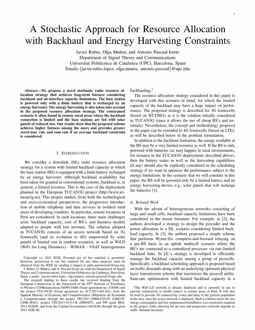
One of the novelties of this work is that we account fora maximum backhaul rate constraint. However, instead oflimiting the instantaneous access network data rates as themaximum flow allowed by the backhaul, as in [2], [3], and [9],we limit the average throughput served by the access network.That means that we allow the instantaneous rate in the accesswireless links to surpass the backhaul limitation at certain timeinstants. This can be done whenever we have queues at theentrance of the access network and such queues are stable(which, in fact, is guaranteed by imposing that the averageaggregated rate is not higher than the backhaul capacity).As we focus on fairness, in the resource allocation problemthe long-term backhaul capacity is equally divided among theusers with the same type of service. Accordingly, we considerin the access network resource allocation problem that thebackhaul capacity is equally divided among the users with thesame type of service. Fig. 1 presents the system architectureof the target rural scenario.

B. Power Consumption Model and Battery Dynamics

In this subsection, we introduce the power consumption andbattery model considered in this paper. The overall powerconsumption at the BS is modeled as the addition of theradiated power, which is divided into the power devoted topilot channels (PCPICH assumed to be fixed) and the powerconsumed by the traffic channels (PBS(t)), and a fixed powerconsumed by the electronics of the BS (Pc), where t denotesthe scheduling period. The model considered for the last termis based on [12] and includes the power consumption of theradio frequency (RF) chains, the baseband power consumption,and the consumption of the cooling systems. The maximum

3

core network

coverage area of the access BS

Fig. 1. Architecture of the target rural scenario under consideration in thepaper. The BS is powered with a solar panel and a battery and the backhaulconsidered is based on WiFi-LD. The specific details of the real deploymentas well as the location are explained in the simulation section.

traffic power will depend on the current battery level of theBS, as will be described in more detail later.

The overall energy consumption by the BS during the t-thscheduling period is

E(t) , Ts · (PCPICH + PBS(t) + Pc) , ∀t, (1)

where Ts is the duration of the scheduling period. Due tophysical constraints of the amplifiers of the BS, the amount ofpower available for traffic services is limited, and it is denotedas Pmax

BS , so PBS(t) ≤ PmaxBS .

Let B(t) be the energy stored at the battery of the BS atthe beginning of the scheduling period t. Then at period t+1,the battery level is updated in general as

B(t+ 1) = f(B(t), E(t), H(t)), ∀t, (2)

where H(t) is the energy harvested in Joules during thescheduling period t and the function f(·) : R+ × R+ ×R+ → R+ depends upon the battery dynamics, such asstorage efficiency and memory effects. A common practiceis to consider the following battery update:

B(t+ 1) = (B(t)− E(t) +H(t))Bmax

0 , ∀t, (3)

where (x)ba is the projection of x onto the interval [a, b],i.e., (x)ba = min{max{a, x}, b}, which accounts for possiblebattery overflows and assures that the battery levels are non-negative, and Bmax is the battery capacity. Notice that thewhole harvesting collected during period t is assumed to beavailable in the battery at the end of the period for simplicity.In general, the total energy consumed by the BS during oneperiod will be limited by a function of the current battery levelas

Ts · (PCPICH + PBS(t) + Pc) ≤ g(B(t)), ∀t, (4)

where the function g(·) is defined as g(B(t)) ,min{Ts (PCPICH + Pmax

BS + Pc) , w(B(t))}, and w(·) : R+ →R+ a generic continuous increasing function that satisfiesw(B(t)) ≤ B(t), ∀t. For example, if all the battery is allowedto be spent during one particular epoch, then w(B(t)) = B(t).Nevertheless, the approach followed in this paper is to limitthe amount the battery that can be used in order to keep more

energy in the battery over long periods of time. Thus, only agiven fraction of the battery is allowed to be used during aparticular scheduling period, i.e.,

w(B(t)) = α ·B(t), 0 ≤ α ≤ 1. (5)

C. Energy Harvesting Model

We assume a discretized model for the energy arrivals [13]where H(t) is modeled as an ergodic Bernoulli process (whichis a particular case of a Markov chain). As a result, only twovalues of harvested energy are possible, i.e., H(t) ∈ {0, e},where e is the amount of Joules contained in an energypacket. The probability of receiving an energy harvestingpacket during one scheduling period depends on the actualharvesting intensity (in the case of solar energy, it dependson the particular hour of the day) and is denoted by p(t).Note that a higher value of p(t) will be obtained in schedulingperiods where the harvesting intensity is higher, e.g., duringsolar presence such as during the day, and a lower value ofp(t) will be obtained during periods of solar absence, such asduring the night.

D. System Assumptions

Let us collect all the channel gains, hk, that includes theantenna gains, the path loss, and the fading, in h = {hk, ∀k ∈KV ∪ KD}. Generally, the wireless channels depend on thespecific scheduling period, h(t), as they vary over time but,for simplicity in the notation, we will just refer to them as hthroughout the paper. The traffic power, PBS(t) from (1), canbe split into power for voice and data connections as PBS(t) =∑k∈KV pk(h) +

∑k∈KD pk(h), where pj(h) and pk(h) are

the instantaneous powers corresponding to the transmissiontoward the j-th and k-th voice and data user, respectively. LetPRAD(t) = PBS(t) + PCPICH be the overall radiated power bythe BS.

The voice users request a fixed data rate and we assume thatjust one WCDMA code is assigned to them. This is translatedinto a minimum signal to interference and noise ratio (SINR)requirement as follows:

MV pk(h)hkθ(PRAD(t)− pk(h))hk + σ2

≥ Γ, ∀k ∈ KV , (6)

where MV is the spreading factor for voice codes, θ is theorthogonality factor among DL codes [11], and σ2 is the noisepower. For simplicity in the notation and tractability, we willconsider the following approximation2:

θ(PRAD(t)− pk(h))hk + σ2 ≈ θPRAD(t)hk + σ2. (7)

On the other hand, the data users request a flexible servicerate. The instantaneous throughput in the wireless accesschannel achieved during one particular scheduling period bythe k-th user, rk(h), is upper bounded by the maximum

2If the number of users is relatively high, then PRAD(t) � pk , and theapproximation is fair. In any case, the approximation provides a lower boundof the actual SINR value.

4

achievable rate that the access network is able to provide,which is formulated as

rk(h) ≤ nk(h)W

MDlog2

(1 +

MDpk(h)hknk(h)(θPRAD(t)hk + σ2)

),

(8)where MD is the spreading factor for data codes, W is thechip rate, and nk(h) is the number of codes assigned to userk. Notice that we have also approximated the denominatorwithin the logarithm as in (7).

III. PROBLEM FORMULATION

Let us introduce the following set of definitions: r ,{rk(h), ∀k ∈ KD}, p , {pk(h), ∀k ∈ KV }, p ,{pk(h), ∀k ∈ KD}, n , {nk, (h) ∀k ∈ KD}. We formulatean optimization problem for the resource allocation strategywith backhaul and energy constraints to be executed at thebeginning of each particular scheduling period, which involvesfinding the optimum resource allocation variables, r, p, p, andn that maximize the minimum of the expected throughputs(note that if a scheduling criterion different from the maximinapproach is to be taken, problem (9) could be extended by justreformulating the objective function accordingly):

maximizer, p, p, n, PRAD(t)

mink∈KD

Eh[rk(h)] (9)

subject to

C1 :MV pk(h)hk

θPRAD(t)hk + σ2≥ Γk, ∀k ∈ KV

C2 : Eh[rk(h)] ≤ RBH − RBH(|KV |)ξ|KD|

, ∀k ∈ KD

C3 : rk(h) ≤ nk(h)W

MDlog2

(1 +

MDpk(h)hknk(h)(θPRAD(t)hk + σ2)

)C4 : Ts

( ∑k∈KV

pk(h) +∑k∈KD

pk(h)

)≤ φ (B(t))

C5 :∑k∈KD

nk(h) ≤ Nmax

C6 : rk(h) ≥ 0, pk(h) ≥ 0, nk(h) ≥ 0, ∀k ∈ KDC7 : PRAD =

∑k∈KV

pk(h) +∑k∈KD

pk(h)

where ξ, (ξ > 1), is an overhead considered for the datatransmissions to be sent through the backhaul, RBH(|KV |) isthe backhaul capacity used by the voice users3, |KV | being thenumber of voice users, RBH is the overall backhaul capacity,Γ is the target SINR for the voice users, the function φ(·) is re-lated to g(·) in (4) as φ (B(t)) = g(B(t))−Ts ·(PCPICH + Pc),and Nmax is the number of available codes for the data users.Although all the variables in the optimization problem (9)depend on the scheduling period t, we only keep such explicitdependence w.r.t. time in the variable PRAD(t) to make explicitthat the temporal evolution of the battery levels has a direct

3The overall backhaul capacity required to provide voice service generallydepends on the current number of voice users being served. In some cases,voice users can be jointly encoded and, thus, the overall overhead for voiceusers may be reduced as the number of voice users increases. Anyway, inthe problem formulation and the for the sake of generality, we just use thenotation RBH(|KV |).

impact on the maximum power to be spent for the voice anddata traffic, which is not constant over time.

It is important to realize that problem (9) may not be feasibledue to constraint C1 as it may happen that there could not beenough power to satisfy all the target SINRs simultaneously.However, let us consider initially through the developmentthat the problem is feasible (the feasibility condition willbe developed later on). Notice that, at the optimum, C4 isattained with equality; otherwise, we could re-scale all thepower variables with a common positive factor higher than1 until C4 is fulfilled with equality. This would increase theobjective function and all the other constraints would still befulfilled. Because of this, we can assume that the optimumvalue of PRAD(t) is P ?RAD(t) = φ(B(t))

Ts+ PCPICH and we can

eliminate constraint C7 from problem (9). Constraint C2 statesthat the average throughput that a user is experiencing in theaccess network should not exceed the maximum backhaul rateassigned to this user (every user has been already assigned aportion of the backhaul, as commented above). If this is notthe case, then C2 could be rewritten as

∑k∈KD Eh[rk(h)] ≤

RBH−RBH(|KV |)ξ . In any case, notice that the instantaneous

rates allocated to one user in the access network can be higherin some scheduling periods than the maximum backhaul per-user rate

(RBH−RBH(|KV |)

ξ|KD|

)thanks to the fact that queues are

considered at the entrance of the access network. The averagerate constraint C2 assures that the queues will be stable.

Notice that the problem is separable into voice and datausers without loss of optimality. This is because the voiceusers do not affect explicitly the optimal value of the objectivefunction. Thus, we can obtain the optimum power variables forthe voice users (i.e., the minimum power required to satisfyconstraints C1) and, then, assign the rest of the resources tothe data users. Hence, we will start by analyzing the resourceallocation for the voice users in Section III-A.

Let us first provide the guidelines to reformulate the prob-lem presented in (9) for an LTE system, which uses OFDMAas the underlying physical multiple access technology. Theobjective function could be expressed as it is. Constraints C2,C4, and C6 would remain equal (in fact, in C6 nk(h) wouldhave to be changed by the variable representing the number ofcarriers). Constraint C1 needs to be modified. Neither the codegain (MV ) nor the intra-cell interference (as the access is noworthogonal) should be considered. We need to reformulate C3completely. A possible candidate for the power-rate expressionwould be

∑Nj=1 β

jkW log

(1 +

pjk(h)hjkσ2

), where βjk is a new

binary optimization variable that takes a value equal to 1if carrier j is assigned to user k and and value equal to 0otherwise, pjk(h) represents the power per carrier, and W is thecarrier bandwidth. Finally, C5 and C7 would not be present.New constraints would have to be added:

∑∀j,∀k β

jk ≤ N ,

where N is number of available carriers,∑∀k β

jk = 1, ∀j,

and βjk = {0, 1}.

5

A. Resource Allocation for Voice Users

Voice users must satisfy a minimum SINR constraint thatis related to the target data rate service:

MV pk(h)hkθP ?RAD(t)hk + σ2

≥ Γ, ∀k ∈ KV . (10)

It is straightforward to obtain the optimum power allocationfor each voice user as follows (realizing that at the optimum,constraints C1 are fulfilled with equality):

p?k(h) =Γ(θP ?RAD(t)hk + σ2)

MV hk, ∀k ∈ KV . (11)

At this point, we could check the feasibility of (9). Theproblem is feasible if

Ts∑k∈KV

p?k(h) ≤ φ(B(t)), (12)

which could also be written only in terms of the channels ofthe voice users, the current battery level, and some constantsas follows: ∑

k∈KV

1

hk≤ κ1φ(B(t))− κ2, (13)

where κ1 = MV −|KV |θΓσ2TsΓ

and κ2 = |KV |θPCPICHσ2 . If the problem

is not feasible, then we should consider reducing such mini-mum SINR requirements (which would increase the constantterm κ1), dropping out some voice users in the schedulingperiod, or increasing φ(B(t)) by taking a higher value for α,but always guaranteeing that the maximum radiated constraintPmax

BS is not exceeded.

B. Resource Allocation for Data Users

Now that we have considered the voice users, we cantackle the resource allocation problem for the data users bysolving problem (9). Note that problem (9) is convex oncewe know P ?BS(t). To solve problem (9), we will reformulate itby introducing the slack variable s, which preserves convexity[14], as

maximizes, r, p, n

s (14)

subject to C2, . . . , C6 of problem (9)C8 : s ≤ Eh[rk(h)], ∀k ∈ KD

C9 : 0 ≤ s ≤ RBH − RBH(|KV |)ξ|KD|

.

Notice that we have introduced an additional constraint,C9. As is clear from the formulation, this constraint doesnot affect the optimum solution, but it will help in thenumerical search of the optimum value of the new slackvariable s. Notice also that the previous optimization problemis time-coupled (we require the future channel realizationsdue to the expectation operator appearing in C8). In orderto deal with such a difficult problem involving expectations,we propose to use a stochastic approximation [10]. In thisapproach, the constraints involving expectations are dualized,and their Lagrange multipliers are estimated stochasticallyat each period. Let us start by dualizing constraint C8. Let

λ , {λk, ∀k ∈ KD} be the vector of Lagrange multipli-ers associated with C8. The partial Lagrangian is given byLC8(s,λ) = −s+

∑k∈KD λk (s− Eh[rk(h)]). In order to find

the optimum s we have to perform the following minimization:

minimize0≤s≤RBH−RBH (|KV |)

ξ|KD|

LC8(s,λ). (15)

According to [10], when the objective function is lin-ear in the optimization variable, the stochastic primal-dualalgorithms present some numerical problems. This can beavoided by transforming the objective function introducing ageneral differentiable monotonically increasing cost functionU(·) (e.g., the logarithm). Note that the introduction of thisfunction does not modify the optimal value of the optimizationvariables (i.e., the solution is the same). Given that, setting thegradient to zero, ∇sLC8(s,λ) = 0 and solving yields:

s?(λ) =

((U)−1

( ∑k∈KD

λk

))RBH−RBH (|KV |)ξ|KD|

0

, (16)

where U(·) is the derivative of U(·) and (U)−1(·) is theinverse function of U(·). Once we know the optimum s?, theproblem (14) is updated as follows (where we have skippedin the objective function the term that does not depend on theoptimization variables remaining in the optimization problem):

maximizer, p, n

∑k∈KD

λkEh[rk(h)] (17)

subject to C2, . . . , C6 of problem (9).

Now, we proceed to dualize constraint C2. Let µ , {µk, ∀k ∈KD} be the vector of Lagrange multipliers associated with C2.The partial Lagrangian is

LC2(rk(h);λ,µ) = (18)

−∑k∈KD

λkEh[rk(h)]

+∑k∈KD

µk

(Eh[rk(h)]− RBH − RBH(|KV |)

ξ|KD|

),

=−Eh

[ ∑k∈KD

(λk − µk)rk(h)

](19)

−∑k∈KD

µk

(RBH − RBH(|KV |)

ξ|KD|

).

For given Lagrange multipliers λ and µ, the optimizationproblem (14) is equivalently reformulated as (where we haveskipped again in the objective function the term that doesnot depend on the optimization variables remaining in theoptimization problem):

maximizer, p, n

∑k∈KD

(λk − µk)rk(h) (20)

subject to C3, . . . , C6 of problem (9).

Notice that the expectations are no longer present in theformulation because the remaining constraints C3 − C6 areapplied to instantaneous resource allocation variables (with-out expectations) and also because the maximization of the

6

λ(q+1)k =

(λ

(q)k + ε

(s?(λ(q))− Eh

[r?k

(h;λ(q),µ(q)

)]))∞0, ∀k, (21)

µ(q+1)k =

(µ

(q)k + ε

(Eh

[r?k

(h;λ(q),µ(q)

)]− RBH − RBH(|KV |)

ξ|KD|

))∞0

, ∀k, (22)

λk(t+ 1) = (λk(t) + ε (s?(λ(t))− r?k(h;λ(t),µ(t))))∞0 , ∀k, (23)

µk(t+ 1) =

(µk(t) + ε

(r?k(h;λ(t),µ(t))− RBH − RBH(|KV |)

ξ|KD|

))∞0

, ∀k. (24)

maximizep, n

∑k∈KD

(λk(t)− µk(t))nkW

MDlog2

(1 +

MDpkhknk(θP ?RAD(t)hk + σ2)

)(25)

subject to C4, . . . , C6 of problem (9).

expected value of the objective function with respect to r, p,and n in the current scheduling period, in this case, is thesame as the maximization of the term within the expecta-tion. The problem now resides in the computation of theoptimum Lagrange multipliers which requires knowing thestatistics of rk(h). If we solve the dual problem of (20), i.e.,supλ�0,µ�0 inf L(r, p, n,λ,µ), where � means element-wise inequality and the Lagrangian, L, is defined in AppendixA, using a gradient approach, the optimum multipliers could becalculated recursively as shown in (21) and (22) [14], where εis the step size. Note that it is not possible to compute the valueof the Lagrange multipliers in real time and then solve (20),as they depend on the statistics of rk(h) that is a function notknown a priori (it is the solution of the optimization problemitself). In this situation, we propose to follow a stochasticapproximation [10] and eliminate this uncertainty constraintby estimating the multipliers stochastically at each schedulingperiod (with a noisy instantaneous unbiased estimate of thegradient) as shown in (23) and (24) (note that this philosophyis similar to the instantaneous estimation of the gradient in theclassical LMS algorithm [15]).

The advantages of the stochastic techniques are threefold:i) the computational complexity of the stochastic technique issignificantly lower than that of their off-line counterparts; ii)stochastic approaches can deal with non-stationarity environ-ments; iii) the distribution of the involved random variables his not required.

Once we update the values of the Lagrange multipliers,problem (20) can be solved using, for example, a primal-dual approach. Notice that constraint C3 can be putdirectly in the objective function as, at the optimum,it is fulfilled with equality, i.e., r?k(h;λ(t),µ(t)) =

n?k(h;λ(t),µ(t)) WMD

log2

(1 +

MDp?k(h;λ(t),µ(t))hk

n?k(h;λ(t),µ(t))(θP?RAD(t)hk+σ2)

).

Thus, the resource allocation problem to be solved at thebeginning of the scheduling period t is the one shown in (25).Notice that we have not considered the dependency of theoptimization variables with respect to the channels explicitlyfor the sake of simplicity in the notation. Problem (25) canbe solved using, for example, a primal-dual approach, as it isdescribed in Appendix A.

It can be shown that the sample average of the stochasticrates, r?k(h;λ(t),µ(t)), satisfies all the constraints in (9) andincurs minimal performance loss relative to the optimal (off-line) solution of (9). This can be stated rigorously as follows:define F (t) , mink∈KD

1t

∑tτ=1 r

?k(h;λ(τ),µ(τ)) and f? as

the minimum value of the objective function in (9). Then, itholds with probability one that as t → ∞: i) the solutionis feasible; and ii) F (t) ≤ f? + δ(ε), where δ(ε) → 0 asε → 0. A proof of this result is not presented here due tospace limitations but it can be derived following [10]. Letus introduce some important remarks here regarding problem(25):

Remark 1: the values of {λk} measure how far the averagerate s?(λ(t)) is from the instantaneous rates served to theusers in the access network. If the quality of the channelsor the available powers are such that the instantaneous ratesserved in the access network are far from the target averagerate s?(λ(t)) for all the users, the sum of {λk} will increaseand the system will reduce the target average rate s?(λ(t)).

Remark 2: in the access network, the values of {λk} arein charge of ensuring that all average rates tend to growsimultaneously (maximin objective function). Note that, ifat any temporal period s?(λ(t)) > r?k(h;λ(t),µ(t)), thenλk(t+ 1) grows and the priority of the k-th user to be servedincreases.

Remark 3: if at any temporal period r?k(h;λ(t),µ(t)) >RBH−RBH(|KV |)

ξ|KD| , then µk(t + 1) > µk(t). For a fixed set of{λk}, if λk(t+ 1)−µk(t+ 1) decreases, the user will have alower priority to be served in the next period. The same reason-ing could be applied if r?k(h;λ(t),µ(t)) < RBH−RBH(|KV |)

ξ|KD|to deal with the reverse situation.

C. Resource Allocation Algorithm

In this subsection, we present the overall algorithm thatsolves the resource allocation for the voice and data usersbased on the approaches presented in previous sections. Thisalgorithm should be solved by the BS at the beginning of eachscheduling period (whose duration is chosen usually accordingto the channel dynamics). The algorithm is summarized inTable I. Notice that in the algorithm, steps 7 to 15 correspond

7

TABLE IALGORITHM FOR SOLVING RESOURCE ALLOCATION PROBLEM (9)

1: initialize λk(t) ≥ 0, µk(t) ≥ 0, ∀k ∈ KD2: compute P ?RAD(t) = φ(B(t))

Ts+ PCPICH

3: Voice users4: compute p?k(h) =

Γ(θP?RAD(t)hk+σ2)

MV hk, ∀k ∈ KV

5: if Ts∑k∈KV

p?k(h) > φ(B(t)) −→ drop some voice users or reduce Γ, then go to 46: Data users7: repeat8: initialize n � 0

9: repeat10: p

(q,k+1)k = p?k

(n(q,k), β(q),λ(t),µ(t)

)using (27), ∀k ∈ KD

11: n(q,k+1)k = n?k

(n(q,k), p(q,k+1), ϕ(q),λ(t),µ(t)

)using fixed-point iteration in (28), ∀k ∈ KD

12: until p(q,k+1)k and n(q,k+1)

k converge13: update the dual variables, β(q+1) and ϕ(q+1), using p(q)

k and n(q)k with (30) and (31)

14: until β(q+1) and ϕ(q+1) converge15: compute r?k(h;λ(t),µ(t)) with p?k(n, β) and n?k(p, n, ϕ)

16: update (dualized) primal variable:

17: s?(λ(t)) =(

(U)−1(∑

k∈KDλk(t)

))RBH−RBH (|KV |)ξ|KD|

0

18: update stochastic dual variables:19: λk(t+ 1) = (λ(t) + ε (s?(λ(t))− r?k(h;λ(t),µ(t))))∞0

20: µk(t+ 1) =(µ(t) + ε

(r?k(h;λ(t),µ(t))− RBH−RBH (|KV |)

ξ|KD|

))∞0

21: update battery with consumed energy and harvesting:22: B(t+ 1) = (B(t)− E(t) +H(t))B

max

0

23: t←− t+ 1 and go to 2

to the steps presented in Appendix A to solve the convexoptimization problem (25). Note also that the computationalburden of the proposed scheme is similar to the one of theconventional PF approach [16]. In steps 10 and 11, we needto solve two waterfilling-like expressions, and the rest of thesteps are just simple updates.

IV. NUMERICAL EVALUATION

In this section we evaluate the performance of the proposedstrategy. The scenario under consideration is composed of 1BS, 3 voice users, and 6 data users. The maximum radiatedpower is Pmax

BS = 9 dBm, the pilot power is PCPICH = 4 dBm(which represents the 13% of the maximum radiated power,as we considered in [17]), and the fixed power is Pc = 3 dBm(considering the model in [12], which was applied in [17]).The number of available codes for data transmission servicesis Nmax = 15. All the users are mobile with a speed of 3m/s. The instantaneous channel gain, hk, incorporates antennagains, Rayleigh fading with unitary power, and the path loss.The path losses correspond to a town in Peru known as SanJuan (see details in [17]). The orthogonality factor is θ = 0.35.The code gain of data codes MD = 16 and the minimum SINRnormalized with code gain for voice users is, Γ

MV= −13.7 dB

which corresponds to a rate of 12.2 Kbps. The noise power isσ2 = −102 dBm. The battery capacity is Bmax = 410 µJ, theenergy packet size is e = 30 µJ, and α = 0.3 unless otherwisestated. The scheduling period for the data users and voice usersare 2ms and 20ms, respectively, thus, Ts = 2 ms. The utility

function is U(·) = log(·). Two backhaul capacities have beenconsidered in the simulations: RBH = 2 Mbps and RBH =500 Kbps. The amount of backhaul capacity required by the3 voice users considered in this deployment is RBH(|KV |) =173 Kbps. The overhead for the data transmissions is ξ = 1.2.The step size for the update of the stochastic multipliers isε = 10−3. For a more detailed description of the simulationparameters see [17].

In the simulations, we consider as a benchmark the casewhere the BS is connected to the electric grid (which meansequivalently that the battery remains full of energy for thewhole simulation). For comparison purposes, we also show theresource allocation of the proposed strategy and the PF strat-egy both with an instantaneous per-user backhaul constraintrk(h) ≤ RBH−RBH(|KV |)

ξ|KD| . Thanks to this, we can comparethe performance of the stochastic maximin strategy with well-known scheduling strategies and we can directly measure theimprovement of the proposed stochastic scheme when weallow instantaneous access data rates to surpass the backhaulcapacity. The effective length of the exponential window in thePF scheme has been set to Tc = 500 [16]4. In the figures, PErefers to the solution of Algorithm 9, PI refers to the strategyfrom (9) but replacing constraint C2 by an instantaneousbackhaul constraint, and PF refers to the proportional fair.

4The weights of the PF scheduler are calculated as ωk(t) = 1Tk(t)

,where Tk(t) is the average throughput of user k computed as Tk(t) =(1− 1

Tc)Tk(t− 1) + 1

Tcrk(t).

8

0 1000 2000 3000 4000 50000

2

4

6

8 x 106

Scheduling periods

bit/s

Instantaneous rate user 1Backhaul rate per user

0 1000 2000 3000 4000 50000

2

4

6

8 x 106

Scheduling periods

bit/s

Instantaneous rate user 2Backhaul rate per user

0 1000 2000 3000 4000 50000

2

4

6

8 x 106

Scheduling periods

bit/s

Instantaneous rate user 4Backhaul rate per user

0 1000 2000 3000 4000 50000

2

4

6

8 x 106

Scheduling periods

bit/s

Instantaneous rate user 6Backhaul rate per user

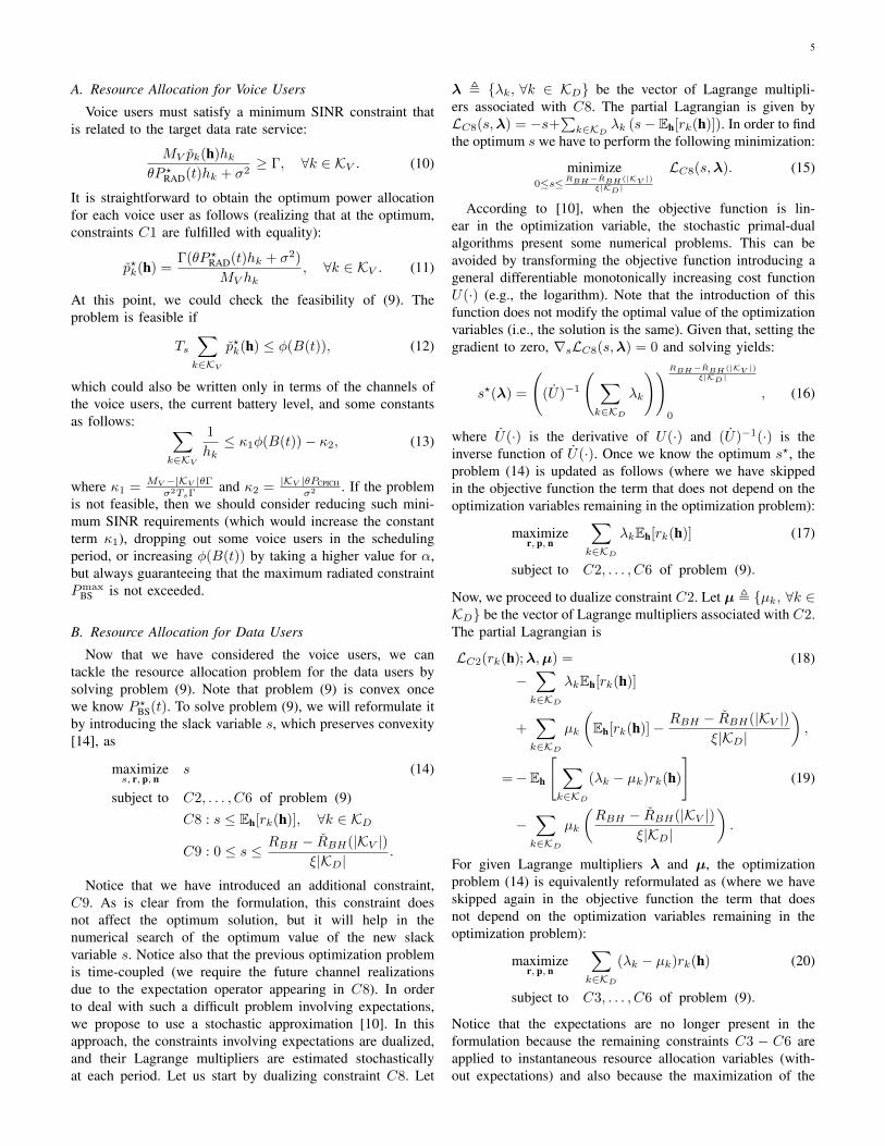
Fig. 2. Time evolution of the instantaneous data rates served at the accessnetwork and the backhaul capacity limitation per user with a backhaul capacityof 2 Mbps.

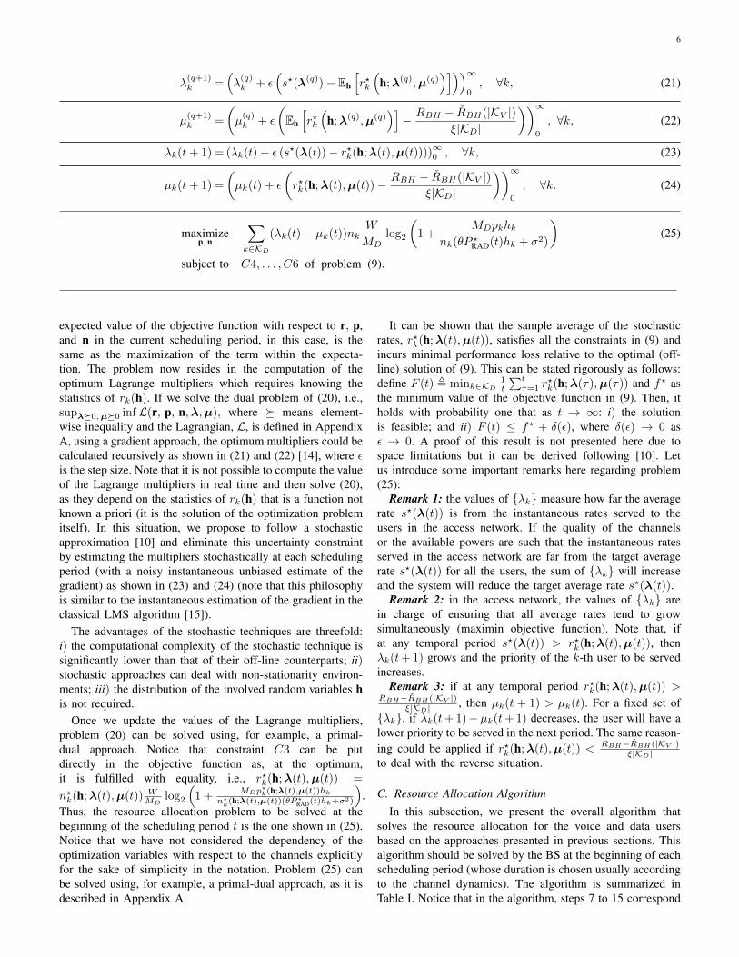
Fig. 2 presents the instantaneous data rates served at theaccess network of four data users out of the six. In this case,the BS is connected to the electric power grid. As we cansee, the instantaneous rates are able to exceed the backhaulcapacity in particular scheduling periods whereas, at the sametime, the average rates fulfills the maximum backhaul capacityas it is shown in Fig. 3. Fig. 3 shows the time evolutionof the expected data rates of the three approaches. At anytime instant the expected rates have been estimated usingrk(t) = 1

t

∑tτ=1 rk(τ). We also plot the time evolution of

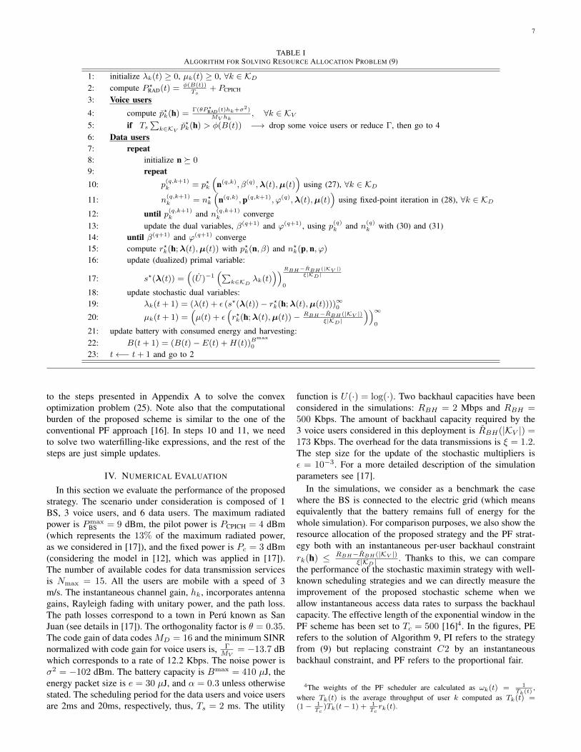
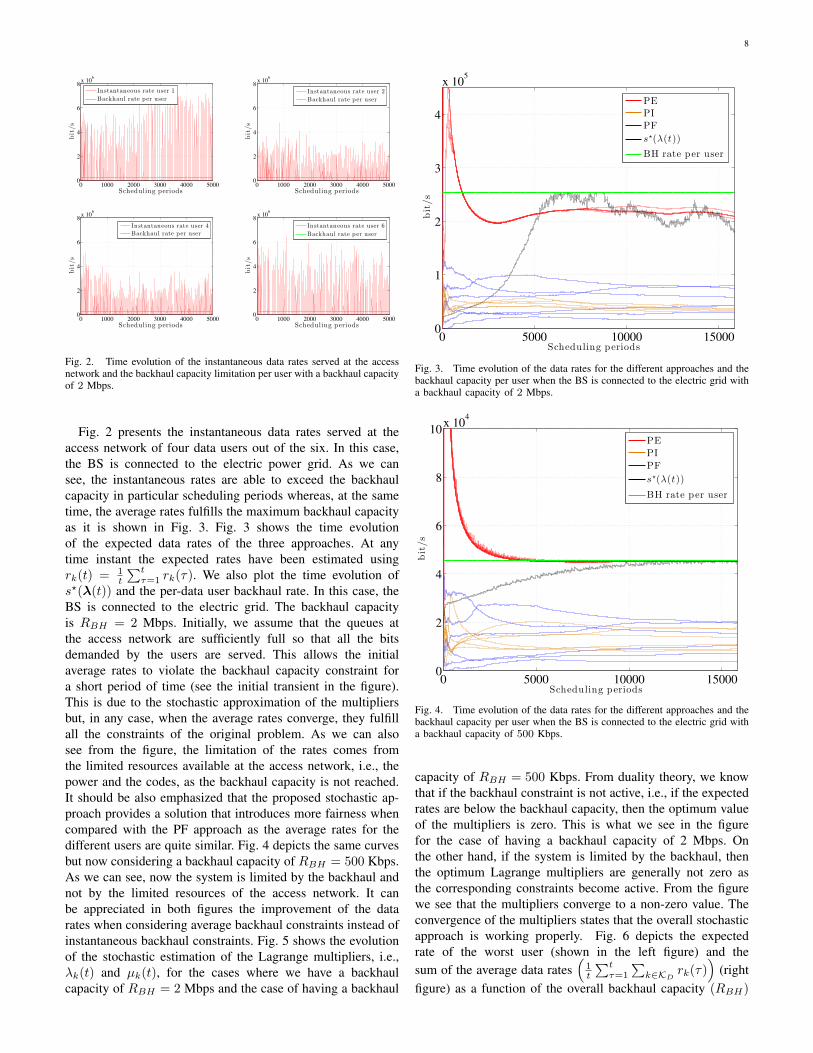
s?(λ(t)) and the per-data user backhaul rate. In this case, theBS is connected to the electric grid. The backhaul capacityis RBH = 2 Mbps. Initially, we assume that the queues atthe access network are sufficiently full so that all the bitsdemanded by the users are served. This allows the initialaverage rates to violate the backhaul capacity constraint fora short period of time (see the initial transient in the figure).This is due to the stochastic approximation of the multipliersbut, in any case, when the average rates converge, they fulfillall the constraints of the original problem. As we can alsosee from the figure, the limitation of the rates comes fromthe limited resources available at the access network, i.e., thepower and the codes, as the backhaul capacity is not reached.It should be also emphasized that the proposed stochastic ap-proach provides a solution that introduces more fairness whencompared with the PF approach as the average rates for thedifferent users are quite similar. Fig. 4 depicts the same curvesbut now considering a backhaul capacity of RBH = 500 Kbps.As we can see, now the system is limited by the backhaul andnot by the limited resources of the access network. It canbe appreciated in both figures the improvement of the datarates when considering average backhaul constraints instead ofinstantaneous backhaul constraints. Fig. 5 shows the evolutionof the stochastic estimation of the Lagrange multipliers, i.e.,λk(t) and µk(t), for the cases where we have a backhaulcapacity of RBH = 2 Mbps and the case of having a backhaul

0 5000 10000 150000

1

2

3

4

x 105

Scheduling periods

bit/s

PEPIPF

s⋆(λ(t))

BH rate per user

Fig. 3. Time evolution of the data rates for the different approaches and thebackhaul capacity per user when the BS is connected to the electric grid witha backhaul capacity of 2 Mbps.

0 5000 10000 150000

2

4

6

8

10x 10

4

Scheduling periods

bit/s

PEPIPF

s⋆(λ(t))

BH rate per user

Fig. 4. Time evolution of the data rates for the different approaches and thebackhaul capacity per user when the BS is connected to the electric grid witha backhaul capacity of 500 Kbps.

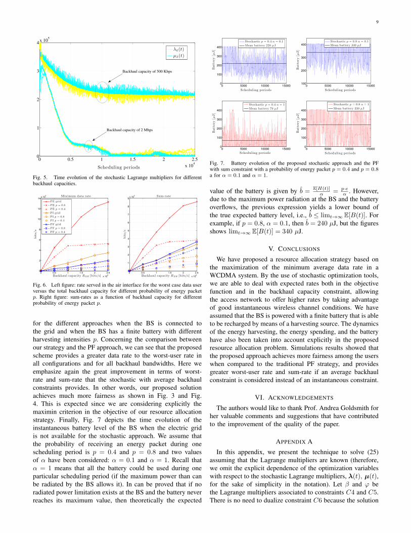
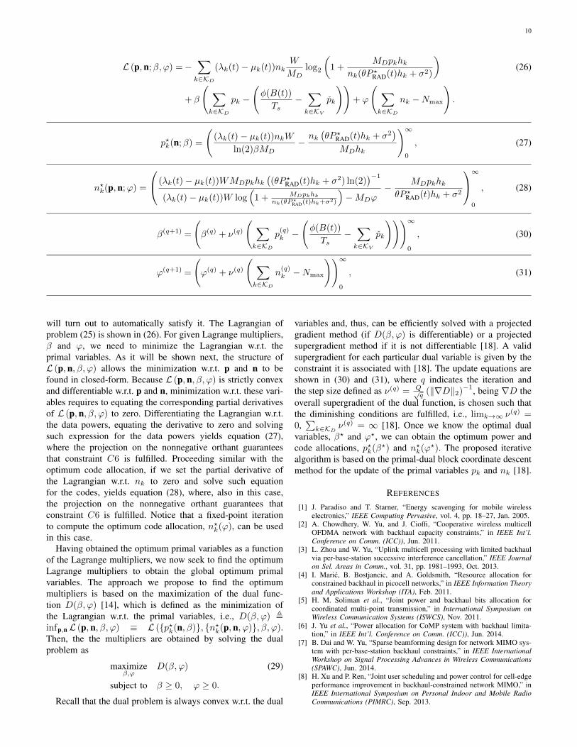
capacity of RBH = 500 Kbps. From duality theory, we knowthat if the backhaul constraint is not active, i.e., if the expectedrates are below the backhaul capacity, then the optimum valueof the multipliers is zero. This is what we see in the figurefor the case of having a backhaul capacity of 2 Mbps. Onthe other hand, if the system is limited by the backhaul, thenthe optimum Lagrange multipliers are generally not zero asthe corresponding constraints become active. From the figurewe see that the multipliers converge to a non-zero value. Theconvergence of the multipliers states that the overall stochasticapproach is working properly. Fig. 6 depicts the expectedrate of the worst user (shown in the left figure) and thesum of the average data rates

(1t

∑tτ=1

∑k∈KD rk(τ)

)(right

figure) as a function of the overall backhaul capacity (RBH)

9

0 0.5 1 1.5 2 2.5

x 104

0

1

2

3

4x 10

5

Scheduling periods

λk(t)

µk(t)

Backhaul capacity of 500 Kbps

Backhaul capacity of 2 Mbps

Fig. 5. Time evolution of the stochastic Lagrange multipliers for differentbackhaul capacities.

0 0.5 1 1.5 2 2.5

x 106

0

2

4

6

8

10

12

14x 10

4

bits/s

Backhaul capacity RBH [bits/s]

Minimum data rate

0 0.5 1 1.5 2 2.5

x 106

0

1

2

3

4

5

6

7

8

9x 10

5

bits/s

Backhaul capacity RBH [bits/s]

Sum-rate

PE grid

PE p = 0.8

PE p = 0.4

PI grid

PI p = 0.8

PI p = 0.4

PF grid

PF p = 0.8

PF p = 0.4

Fig. 6. Left figure: rate served in the air interface for the worst case data userversus the total backhaul capacity for different probability of energy packetp. Right figure: sum-rates as a function of backhaul capacity for differentprobability of energy packet p.

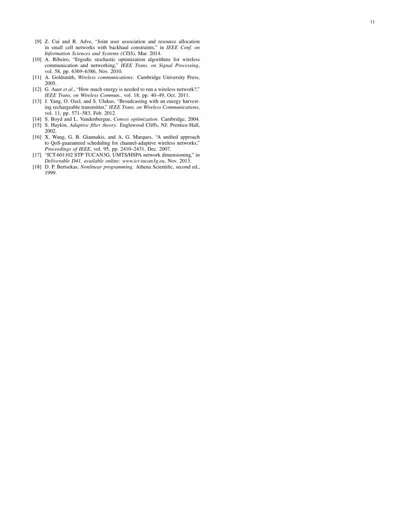
for the different approaches when the BS is connected tothe grid and when the BS has a finite battery with differentharvesting intensities p. Concerning the comparison betweenour strategy and the PF approach, we can see that the proposedscheme provides a greater data rate to the worst-user rate inall configurations and for all backhaul bandwidths. Here weemphasize again the great improvement in terms of worst-rate and sum-rate that the stochastic with average backhaulconstraints provides. In other words, our proposed solutionachieves much more fairness as shown in Fig. 3 and Fig.4. This is expected since we are considering explicitly themaximin criterion in the objective of our resource allocationstrategy. Finally, Fig. 7 depicts the time evolution of theinstantaneous battery level of the BS when the electric gridis not available for the stochastic approach. We assume thatthe probability of receiving an energy packet during onescheduling period is p = 0.4 and p = 0.8 and two valuesof α have been considered: α = 0.1 and α = 1. Recall thatα = 1 means that all the battery could be used during oneparticular scheduling period (if the maximum power than canbe radiated by the BS allows it). In can be proved that if noradiated power limitation exists at the BS and the battery neverreaches its maximum value, then theoretically the expected

0 5000 10000 150000

100

200

300

400

Scheduling periods

Battery[µ

J]

0 5000 10000 150000

100

200

300

400

Scheduling periods

Battery[µ

J]

0 5000 10000 15000100

200

300

400

Scheduling periods

Battery[µ

J]

0 5000 10000 150000

100

200

300

400

Scheduling periods

Battery[µ

J]

Stochastic p = 0.4 α = 0.1

Mean battery 220 µJ

Stochastic p = 0.4 α = 1Mean battery 70 µJ

Stochastic p = 0.8 α = 0.1Mean battery 340 µJ

Stochastic p = 0.8 α = 1

Mean battery 230 µJ

Fig. 7. Battery evolution of the proposed stochastic approach and the PFwith sum constraint with a probability of energy packet p = 0.4 and p = 0.8a for α = 0.1 and α = 1.

value of the battery is given by b = E[H(t)]α = p·e

α . However,due to the maximum power radiation at the BS and the batteryoverflows, the previous expression yields a lower bound ofthe true expected battery level, i.e., b ≤ limt→∞ E[B(t)]. Forexample, if p = 0.8, α = 0.1, then b = 240 µJ, but the figuresshows limt→∞ E[B(t)] = 340 µJ.

V. CONCLUSIONS

We have proposed a resource allocation strategy based onthe maximization of the minimum average data rate in aWCDMA system. By the use of stochastic optimization tools,we are able to deal with expected rates both in the objectivefunction and in the backhaul capacity constraint, allowingthe access network to offer higher rates by taking advantageof good instantaneous wireless channel conditions. We haveassumed that the BS is powered with a finite battery that is ableto be recharged by means of a harvesting source. The dynamicsof the energy harvesting, the energy spending, and the batteryhave also been taken into account explicitly in the proposedresource allocation problem. Simulations results showed thatthe proposed approach achieves more fairness among the userswhen compared to the traditional PF strategy, and providesgreater worst-user rate and sum-rate if an average backhaulconstraint is considered instead of an instantaneous constraint.

VI. ACKNOWLEDGEMENTS

The authors would like to thank Prof. Andrea Goldsmith forher valuable comments and suggestions that have contributedto the improvement of the quality of the paper.

APPENDIX A

In this appendix, we present the technique to solve (25)assuming that the Lagrange multipliers are known (therefore,we omit the explicit dependence of the optimization variableswith respect to the stochastic Lagrange multipliers, λ(t), µ(t),for the sake of simplicity in the notation). Let β and ϕ bethe Lagrange multipliers associated to constraints C4 and C5.There is no need to dualize constraint C6 because the solution

10

L (p,n;β, ϕ) =−∑k∈KD

(λk(t)− µk(t))nkW

MDlog2

(1 +

MDpkhknk(θP ?RAD(t)hk + σ2)

)(26)

+ β

( ∑k∈KD

pk −

(φ(B(t))

Ts−∑k∈KV

pk

))+ ϕ

( ∑k∈KD

nk −Nmax

).

p?k(n;β) =

((λk(t)− µk(t))nkW

ln(2)βMD−nk(θP ?RAD(t)hk + σ2

)MDhk

)∞0

, (27)

n?k(p,n;ϕ) =

(λk(t)− µk(t))WMDpkhk((θP ?RAD(t)hk + σ2) ln(2)

)−1

(λk(t)− µk(t))W log(

1 + MDpkhknk(θP?RAD(t)hk+σ2)

)−MDϕ

− MDpkhkθP ?RAD(t)hk + σ2

∞0

, (28)

β(q+1) =

(β(q) + ν(q)

( ∑k∈KD

p(q)k −

(φ(B(t))

Ts−∑k∈KV

pk

)))∞0

, (30)

ϕ(q+1) =

(ϕ(q) + ν(q)

( ∑k∈KD

n(q)k −Nmax

))∞0

, (31)

will turn out to automatically satisfy it. The Lagrangian ofproblem (25) is shown in (26). For given Lagrange multipliers,β and ϕ, we need to minimize the Lagrangian w.r.t. theprimal variables. As it will be shown next, the structure ofL (p,n, β, ϕ) allows the minimization w.r.t. p and n to befound in closed-form. Because L (p,n, β, ϕ) is strictly convexand differentiable w.r.t. p and n, minimization w.r.t. these vari-ables requires to equating the corresponding partial derivativesof L (p,n, β, ϕ) to zero. Differentiating the Lagrangian w.r.t.the data powers, equating the derivative to zero and solvingsuch expression for the data powers yields equation (27),where the projection on the nonnegative orthant guaranteesthat constraint C6 is fulfilled. Proceeding similar with theoptimum code allocation, if we set the partial derivative ofthe Lagrangian w.r.t. nk to zero and solve such equationfor the codes, yields equation (28), where, also in this case,the projection on the nonnegative orthant guarantees thatconstraint C6 is fulfilled. Notice that a fixed-point iterationto compute the optimum code allocation, n?k(ϕ), can be usedin this case.

Having obtained the optimum primal variables as a functionof the Lagrange multipliers, we now seek to find the optimumLagrange multipliers to obtain the global optimum primalvariables. The approach we propose to find the optimummultipliers is based on the maximization of the dual func-tion D(β, ϕ) [14], which is defined as the minimization ofthe Lagrangian w.r.t. the primal variables, i.e., D(β, ϕ) ,infp,n L (p,n, β, ϕ) ≡ L ({p?k(n, β)}, {n?k(p,n, ϕ)}, β, ϕ).Then, the the multipliers are obtained by solving the dualproblem as

maximizeβ,ϕ

D(β, ϕ) (29)

subject to β ≥ 0, ϕ ≥ 0.

Recall that the dual problem is always convex w.r.t. the dual

variables and, thus, can be efficiently solved with a projectedgradient method (if D(β, ϕ) is differentiable) or a projectedsupergradient method if it is not differentiable [18]. A validsupergradient for each particular dual variable is given by theconstraint it is associated with [18]. The update equations areshown in (30) and (31), where q indicates the iteration andthe step size defined as ν(q) = Q√

q (‖∇D‖2)−1, being ∇D the

overall supergradient of the dual function, is chosen such thatthe diminishing conditions are fulfilled, i.e., limk→∞ ν(q) =0,∑k∈KD ν

(q) = ∞ [18]. Once we know the optimal dualvariables, β? and ϕ?, we can obtain the optimum power andcode allocations, p?k(β?) and n?k(ϕ?). The proposed iterativealgorithm is based on the primal-dual block coordinate descentmethod for the update of the primal variables pk and nk [18].

REFERENCES

[1] J. Paradiso and T. Starner, “Energy scavenging for mobile wirelesselectronics,” IEEE Computing Pervasive, vol. 4, pp. 18–27, Jan. 2005.

[2] A. Chowdhery, W. Yu, and J. Cioffi, “Cooperative wireless multicellOFDMA network with backhaul capacity constraints,” in IEEE Int’l.Conference on Comm. (ICC)), Jun. 2011.

[3] L. Zhou and W. Yu, “Uplink multicell processing with limited backhaulvia per-base-station successive interference cancellation,” IEEE Journalon Sel. Areas in Comm., vol. 31, pp. 1981–1993, Oct. 2013.

[4] I. Maric, B. Bostjancic, and A. Goldsmith, “Resource allocation forconstrained backhaul in picocell networks,” in IEEE Information Theoryand Applications Workshop (ITA), Feb. 2011.

[5] H. M. Soliman et al., “Joint power and backhaul bits allocation forcoordinated multi-point transmission,” in International Symposium onWireless Communication Systems (ISWCS), Nov. 2011.

[6] J. Yu et al., “Power allocation for CoMP system with backhaul limita-tion,” in IEEE Int’l. Conference on Comm. (ICC)), Jun. 2014.

[7] B. Dai and W. Yu, “Sparse beamforming design for network MIMO sys-tem with per-base-station backhaul constraints,” in IEEE InternationalWorkshop on Signal Processing Advances in Wireless Communications(SPAWC), Jun. 2014.

[8] H. Xu and P. Ren, “Joint user scheduling and power control for cell-edgeperformance improvement in backhaul-constrained network MIMO,” inIEEE International Symposium on Personal Indoor and Mobile RadioCommunications (PIMRC), Sep. 2013.

11

[9] Z. Cui and R. Adve, “Joint user association and resource allocationin small cell networks with backhaul constraints,” in IEEE Conf. onInformation Sciences and Systems (CISS), Mar. 2014.

[10] A. Ribeiro, “Ergodic stochastic optimization algorithms for wirelesscommunication and networking,” IEEE Trans. on Signal Processing,vol. 58, pp. 6369–6386, Nov. 2010.

[11] A. Goldsmith, Wireless communications. Cambridge University Press,2005.

[12] G. Auer et al., “How much energy is needed to run a wireless network?,”IEEE Trans. on Wireless Commun., vol. 18, pp. 40–49, Oct. 2011.

[13] J. Yang, O. Ozel, and S. Ulukus, “Broadcasting with an energy harvest-ing rechargeable transmitter,” IEEE Trans. on Wireless Communications,vol. 11, pp. 571–583, Feb. 2012.

[14] S. Boyd and L. Vandenbergue, Convex optimization. Cambridge, 2004.[15] S. Haykin, Adaptive filter theory. Englewood Cliffs, NJ: Prentice-Hall,

2002.[16] X. Wang, G. B. Giannakis, and A. G. Marques, “A unified approach

to QoS-guaranteed scheduling for channel-adaptive wireless networks,”Proceedings of IEEE, vol. 95, pp. 2410–2431, Dec. 2007.

[17] “ICT-601102 STP TUCAN3G, UMTS/HSPA network dimensioning,” inDeliverable D41, available online: www.ict-tucan3g.eu, Nov. 2013.

[18] D. P. Bertsekas, Nonlinear programming. Athena Scientific, second ed.,1999.