A stochastic indicator for sovereign debt sustainability

Jasper Lukkezen and Hugo Rojas-Romagosa*

15 July 2016

AbstractWe propose a stochastic indicator to assess government debt sustainabil-

ity. This indicator combines the effect of economic uncertainty –representedby stochastic simulations of interest and growth rates– with the expected fiscalresponse that provides information on the long-term country specific attitudetowards fiscal sustainability. We apply our framework on post-war data fornine OECD countries and find that our indicator –the potential increase indebt in bad states of the world– distinguishes countries that have sustainabilityconcerns: Italy, Spain, Portugal and Iceland, from those that do not: UnitedStates, United Kingdom, Netherlands, Belgium and Germany.

Keywords: public debt, fiscal policy, debt sustainability, stochastic simulationsJEL Classification: H6, H3, E6

1 IntroductionWhether government debt –and fiscal policy in general– is sustainable in the mediumand long-term has been one of the main topics of debate in the current Euro crisis.An assessment of debt sustainability is a key input in decisions concerning the speedof fiscal consolidation, the need for reform and the determination of risk premia ongovernment debt. Furthermore, fiscal surveillance is a key concern within a mone-tary union, where unsustainable public finances may cause significant cross-borderspillovers.1 There is considerable debate, however, on how to measure debt sustain-

*Lukkezen: Utrecht University Kriekenpitplein 21-22, 3584EC Utrecht, The Netherlands(j.h.j.lukkezen@uu.nl) and Economisch Statistische Berichten; Rojas-Romagosa: CPB NetherlandsBureau for Economic Policy Analysis, Postbus 80510, 2508GM The Hague, The Netherlands(h.rojas-romagosa@cpb.nl). Acknowledgements: The authors would like to thank Nico van Leeuwenfor excellent research assistance; Oscar Bajo Rubio, Henning Bohn, Frits Bos, Carlos Marinheiroand Jan Luijten van der Zanden for making their data available; and two anonymous referees andthe editor of this journal, as well as Leon Bettendorf, Adam Elbourne, Casper van Ewijk, ClemensKool, Catherine Mathieu, Ruud Okker, Bert Smid, Paul Veenendaal and participants at CPB, UUseminars and the Euroframe 2012 conferences, for providing suggestions for improvement. All errorsare our own.

1For an overview of direct spillovers see Lejour et al. (2011), for spillovers via contagion seeArezki et al. (2011) and for spillovers via monetary policy see Beetsma and Giuliodori (2010) andreferences therein.

1

ability. The original sustainability norms envisaged at the creation of the EuropeanMonetary Union (EMU) were to follow the Maastricht Treaty criteria: ceilings of3% and 60% on government deficits and debt-to-GDP ratios, respectively. However,these criteria have proven to be inadequate as several countries violated these cri-teria without consequences, while others that met them have been nonetheless hitby the crisis. In particular, Spain had debt-to-GDP ratios and budget deficits wellbelow these Maastricht limits, but has still suffered sovereign debt problems.

The objective of this paper is to find more informative economic indicators thatprovide guidance on medium- and long-term fiscal sustainability. We develop adynamic framework for the assessment of sustainability of public finances and focuson the question whether governments can be expected to be "in control" of publicfinances. Our approach entails a simple and practical stochastic simulation whichtakes into account the response of fiscal policy to the state of public finances.

Our methodology has two steps. First, we follow Bohn (1998, 2008) and esti-mate a fiscal reaction function (FRF), which provides information on the long-termcountry-specific behaviour of that country’s government and its attitudes towardsfiscal sustainability. A positive and significant FRF coefficient denotes a country thathas been committed to reduce or maintain steady debt-to-GDP ratios conditionalon short-term economic fluctuations and temporary government expenditures.2 Inthe second step, the estimated FRF is combined with the stochastic debt simulationmethod proposed by Celasun et al. (2006) and Budina and van Wijnbergen (2008),which uses historic volatility of interest and growth rates to generate a distributionof future expected debt levels. We then simulate this model ten thousand times togenerate a distribution of debt paths, which can be used to analyse the effect offiscal responses and interest and growth rate volatility on debt-to-GDP ratios.3

The main contribution of this paper is that using this framework we derive astochastic indicator for the assessment of sustainability of government debt. Ourindicator provides insight into the question whether a country is "in control" of itspublic finances. In practical terms, debt can be regarded as sustainable if it doesnot lead to ever diverging debt ratios in the long run –i.e. if the simulated debt-to-GDP distribution is properly defined and bounded (Hall, 2013). We define oursustainability indicator to assess the upward risk associated with the distributionof the simulated future debt levels. In particular, our indicator measures the devi-

2In particular, a positive and significant FRF coefficient can be interpreted as a government thatengages in fiscal austerity to reduce debt levels even when markets are not specifically concernedabout those debt levels, nor is there international pressure (e.g. EU institutions) to reduce them. Areason for engaging in austerity even when not forced might be that fiscally responsible politicianshave larger re-election probabilities in advanced economies (Brender and Drazen, 2005, 2008).

3Medeiros (2012) also combines a VAR with a fiscal reaction function. However, he relies onshorter time series and is therefore restricted to estimate a panel fiscal reaction function that yieldsthe average fiscal response. This approach thus has the limitation that it assumes that each countryhas the same fiscal response, irrespective of institutional settings, policy-maker attitudes towardsdebt and historical precedents. Berti (2013) uses a VAR to capture the shocks as well, she howeverhas no endogenous fiscal response, yet focuses on incorporating central projections for fiscal policy.

2

ation of the distribution’s upper bound with respect to its median.4 Note that weexplicitly avoid using any limit or critical debt level as part of our sustainabilityindicator.5 If the upward risk is large –as reflected in our sustainability indicator–default fears cannot be dismissed as irrational, since after all, the debt level couldrise significantly. A stronger FRF limits upward risk and leads to lower indicatorvalues, reflecting the confidence by market participants that the government willtake the actions necessary to restore financial stability.6 Conversely, more volatileinterest and growth rates increase upward risk as they lead to more uncertainty.

Given the long-term character of a fiscal response, we collected annual historicdata on GDP and government finances for nine OECD countries spanning over acentury: United States, United Kingdom, Netherlands, Belgium, Germany, Italy,Spain, Portugal and Iceland. In this paper we focus on the post Second WorldWar period, using the pre-war data as a robustness check. We find that until the1980s, public debt was reduced by real growth and relatively low -and at timesnegative- real interest rates. In practical terms, this means that in this period itwas not necessary to implement fiscal austerity plans to substantially reduce publicdebt. With financial liberalisation from the 1980s onwards, however, governmentsare less capable of controlling real interest rates and this increased the importance offiscal policy for debt sustainability. We find that for the United States, the UnitedKingdom, the Netherlands, Belgium and Germany the fiscal response to increasesin the debt-to-GDP ratio has been robust and positive for the whole sample aswell as the post-war period. On the other hand, Spain, Portugal and Iceland havenon-significant fiscal responses in the post-war period, which creates doubts abouttheir capacity to reduce debt by fiscal austerity. Italy has a positive and significantfiscal response coefficient, yet has debt sustainability concerns as its high currentdebt level makes it very susceptible to fluctuations in interest and growth rates. Forinstance, the simulated future debt paths for Italy, Spain, Portugal and Iceland showthat their larger interest and growth rate variance requires a relatively large fiscalresponse to prevent debt levels from becoming unsustainable.

Finally, we show that our debt sustainability indicator ("DSI") performs well asan early-warning indicator. When we use only data until 2007 (i.e. prior to thefinancial crisis), we find that our indicator is highly correlated with sovereign risk

4For example, if the distribution of the simulated debt levels is relatively wide, then the probabil-ities of future debt levels to increase substantially are higher than when the distribution is relativelynarrow. This upward risk is captured by a higher level of our sustainability indicator. Technically,our indicator is defined as the difference between the 97.5% upper bound minus the median of thesimulated debt distribution. The use of the 97.5% level is arbitrary, but using values of 95% and99% yield the same qualitatively results.

5Several papers find that debt above a certain level has negative consequences for economicgrowth (Reinhart and Rogoff, 2010; Cecchetti et al., 2011; Checherita-Westphal and Rother, 2012;Égert, 2012; Baum et al., 2013). However, the causality between debt and growth is difficult toestablish and critical debt levels are generally country-specific (e.g. Japan has debt levels wayabove any critical level mentioned in the literature, while other countries had debt crisis well belowthese critical levels), which makes the cross-country results from these studies not informative inan indicator when applied to different countries.

6Bursian et al. (2015) study the role of trust on fiscal reaction functions.

3

premia between 2009 and 2012. Our indicator thus clearly identifies those countriesthat were later hit by the debt crisis: Portugal, Iceland, Italy and Spain. Moreover,it outperforms market based indicators prior to the crisis such as CDS rates in 2007.

An assessment of debt sustainability using this approach can complement exist-ing indicators. Static sustainability indicators, such as the size of public debt orthe budget balance are often used to assess government finances in the short- andmedium term (European Commission, 2012b).7 While these indicators are straight-forward and unambiguous, they provide little information on the uncertainties publicfinances face in the near future. Moreover, these indicators neglect the role of thepolicy maker in controlling public debt. There is ample evidence, however, that theresponsiveness of fiscal policy to economic setbacks and the quality of fiscal institu-tions are essential to debt sustainability. Our approach contributes to this literatureby explicitly modelling the effect of economic uncertainty on medium/long term debtsustainability. Nevertheless, it is important to note that our results are not informa-tive over short-term developments. In particular, our analysis is based on ex-postdata (at least a year old) that already accounts for any endogenous behaviour be-tween fiscal policy, financial markets and the real economy –but these mechanismsare still at play in any short-term debt sustainability assessment and thus, they arebeyond the scope of our analysis.8

The paper is organised as follows. Section 2 presents the theoretical backgroundon debt sustainability. Section 3 describes the data. In Section 4 we elaborate onour empirical strategy and present country-specific econometric results. Section 5describes our stochastic analysis and Section 6 explains how we construct our debtsustainability indicator and how to apply it as an early-warning indicator. Section7 summarises our main results.

2 Fiscal reaction functions and debt sustainabilityWe analyse debt sustainability using the approach developed by Bohn (1998, 2008).In essence, Bohn equates fiscal sustainability with the stationarity of the debt-to-GDP time series –i.e. when the debt-to-GDP time series is stationary over time, thedebt is sustainable. His approach uses historical information on government financesand identifies the channels that determine the path of the debt-to-GDP ratio overtime.

Bohn’s approach uses two equations to determine the evolution of the debt-to-GDP ratio: the accounting equation for debt and a behavioural equation for pri-mary surplus. Both equations are specified with an error-correction for the primary

7See http://ec.europa.eu/economy_finance/economic_governance/index_en for an overviewof European regulations and directives based on such indicators. For the long term, the EuropeanCommission employs projections to assess the sustainability of public finances against the back-ground of ageing populations (European Commission, 2012a).

8Readers interested in short-term behaviour should use indicators from the signals approach(Berti et al., 2012) or resort to structural modelling.

4

surplus-to-GDP ratio and the debt-to-GDP ratio. First, the accounting equation:

𝑑𝑡+1 = 1 + 𝑟𝑡

1 + 𝑦𝑡(𝑑𝑡 − 𝑠𝑡), (1)

which says that the debt-to-GDP ratio at the beginning of period 𝑡 + 1, 𝑑𝑡+1, equalsthe debt-to-GDP ratio at the beginning of period 𝑡 minus the primary surplus-to-GDP ratio over period 𝑡, 𝑠𝑡, times the gross interest rate factor over period 𝑡, 1 + 𝑟𝑡,divided by the change in the GDP over period 𝑡, 1 + 𝑦𝑡.9 For our analysis we usereal growth and interest rates.10

Second, we estimate a behavioural equation for the primary surplus-to-GDPratio, which tells us how the government’s budget responds to debt accumulationgiven a structure of shocks occurring in the background. We estimate the followingregression:

𝑠𝑡 = 𝛼 + 𝜌𝑑𝑡 + 𝛽Z𝑡 + 𝜀𝑡, (2)

where 𝜌 is the fiscal reaction parameter, which indicates whether the governmenthas increased its primary surplus as a reaction to an increase in the debt-to-GDPratio, Z is a set of other primary surplus determinants and 𝜀𝑡 is an error term. Wewill refer to this equation as the fiscal reaction function (FRF).1112

The use of Z is crucial to account for shocks and it consists of two variables:YVAR, a measure of cyclical fluctuations in output (e.g. business cycles); andGVAR, a measure of temporary government spending (e.g. military expenditureduring war periods).13 The presence of these shocks makes it difficult to detect if𝑑 is stationary. Including these variables, hence, is crucial for the results (Bohn,1998).14

9Throughout this paper stock variables are defined at the beginning of the period, whereas flowvariables are defined over the period. Interest rates refer to effective interest rates defined as theproportion of interest payments to the overall government debt level.

10We could have used nominal growth and interest rates as well. Note that the nominal interestrate is given by 𝑖 = (1 + 𝑟)(1 + 𝜋) − 1 with 𝜋 inflation, and the nominal GDP growth rate is givenby 𝑔 = (1 + 𝑦)(1 + 𝜋) − 1. In equation (1) they cancel out to the first order.

11Note that it is also possible to postulate an auto-regressive process for 𝑠𝑡, as in Bartoletto et al.(2013). Then the actual fiscal response is captured by a combination of an auto-regressive and aresponse to debt parameter. We prefer to stay as close as possible to Bohn’s approach and proceedby calculating our fiscal response using autocorrelation consistent estimators in Section 4.

12There is a potential bias in equation (2), which is of limited consequence. If the debt-to-GDPratio has a unit root, the estimated fiscal response coefficient will be biased downwards towardszero. Then, the parameter 𝛿 (to be introduced later) will be biased upwards and we will concludewith even more certainty that debt is not sustainable. If the debt-to-GDP ratio does not have aunit root, our results are unbiased and this does not matter. We added text to bring this pointacross.

13Bohn (1998) uses Barro (1979)’s classical tax-smoothing theory to underpin the use of thesevariables as temporary government expenses and the effects of business cycle slow-downs should befinanced by a higher budgetary deficit.

14From our empirical estimations, however, we find that the crucial variable is YVAR. In oursensitivity analysis, when we drop GVAR and use only YVAR, our main results hold (see Section4.4). Moreover, our results are also robust to the use of lagged YVAR and GVAR variables tocontrol for an unknown form of endogeneity in Equation 2.

5

Substituting equation (2) in (1) yields an expression for the evolution of the debtlevel:

𝑑𝑡+1 = 𝛾𝑡(1 − 𝜌)𝑑𝑡 − 𝛾𝑡 (𝛼 + 𝛽Z𝑡 + 𝜀𝑡) , (3)

where 𝛾 summarises the relationship between interest rates, growth rates and infla-tion:

𝛾𝑡 = 1 + 𝑟𝑡

1 + 𝑦𝑡.

As 𝐸(Z𝑡) = 0, debt sustainability becomes a function of 𝛾 and 𝜌. When we use av-erage values for interest and growth rates (𝑟 and 𝑦, respectively), we can summarisethis information using the parameter 𝛿, such that:

𝛿 = 𝛾(1 − 𝜌) = 1 + 𝑟

1 + 𝑦(1 − 𝜌) (4)

We distinguish three cases:

∙ 𝛿 < 1 implies stationary debt-to-GDP ratios.15 16

∙ 𝛿 > 1 but with 0 < 𝜌 < 𝑟 − 𝑦 implies mildly explosive paths for debt-to-GDPratios (but growing slowly enough to be consistent with IBC).17

∙ 𝛿 > 1 with 𝜌 < 0 and 𝑟 − 𝑦 > 0 characterises exponentially growing debt.

We require, following Bohn (1998, 2008) and Ghosh et al. (2013), a stationaryprocess for the debt-to-GDP ratio – thus 𝛿 < 1. By doing so, we deviate from theliterature that uses unit root or cointegration tests to test whether the intertemporalbudget constraint (IBC) holds.18 As the intertemporal budget constraint holdswhenever there is any corrective action (𝜌 > 0), a mildly explosive debt path is notruled out. This can be problematic as a mildly explosive debt path implies a mildlyexplosive path for the fiscal response (𝜌 times 𝑑) and hence primary surplus as well(Bohn, 2007).

Requiring a stricter condition on sustainability makes the features of the FRFtest not less convenient. Mendoza and Ostry (2008) describe in detail the benefitsand limitations of the FRF analysis. First, it does not require knowledge of the

15Bohn (1998) argues that the coefficient estimates of equation (2) are unbiased if 𝛿 < 1. Heassumes that 𝛾 and 𝛼 + 𝛽Z𝑡 + 𝜀𝑡 are stationary and states that if (1 − 𝜌)𝛾 < 1 then 𝑑 should bestationary. If 𝑑 is stationary, the debt-to-GDP ratio follows a auto-regressive process with near unitroot behaviour and OLS coefficient estimates are unbiased. If (1 − 𝜌)𝛾 > 1, estimates of 𝜌 may bebiased towards zero, which makes debt look even more non-stationary.

16The deterministic steady state debt level can be obtained by writing equation (3) in firstdifferences:

Δ𝑑𝑡+1 = − (1 − 𝛿) 𝑑𝑡 − 𝛾𝛼,

where we use that, by construction, 𝐸(Zt) = 𝐸(𝜀𝑡) = 0. Then the deterministic steady state yields𝑑 = (1 − 𝛿)−1 𝛾𝛼.

17See Bohn (2007) for a formal proof. At the boundary between the first and the second case liesa difference-stationary debt (this is the most studied scenario in the unit root literature).

18See Afonso (2005) for a survey of these type of studies.

6

specific set of government policies on debt, taxes and expenditures. The FRF testdetermines whether the outcome of a given set of policies implicit in the past primarybalance and debt data is in line with fiscal solvency, without knowing the specificsof those policies. Second, since asset pricing applies to all kinds of financial assets,the analysis does not require particular assumptions about debt management, orthe composition of debt in terms of maturity or denomination structure. Third,it relies entirely on ex-post realisations of all our variables. This means that italready contains the outcomes of the endogenous process that interacts governmentalpolicies, financial market assessments and the response of the real economy in theshort-run.

A final remark concerning the FRF analysis is that a time-invariant conditionalresponse of the primary balance to the debt level (𝜌) alone is a sufficient but nota necessary condition for debt sustainability. A non-linear and/or time varyingresponse can also generate fiscal solvency as long as the response is strictly positiveabove a certain debt-to-GDP threshold ratio. This implies that countries withouta positive 𝜌 and with 𝛾 > 0 do not necessarily have unsustainable governmentfinances. Theoretically, they could have a response that kicks in at some higher,not yet reached, debt level or specific set of government policies that will likelyimprove primary surplus in the future. In practical terms, this refers to non-linearrelationships in equation (2), for which we test in our empirical analysis.

What does this analysis tell us about the channels through which the debt levelis controlled? From equation (4) we see that the evolution of the debt ratio is drivenby three contributing channels:19

1. Fiscal reactions. These are captured by the estimated coefficient (𝜌) of theFRF and provide information on the historical fiscal reaction of governments(i.e. changes in primary surpluses) to changes in the debt-to-GDP ratio. Apositive and significant FRF coefficient denotes a country that has been histor-ically committed to reduce or maintain steady debt-to-GDP ratios conditionalon short-term economic fluctuations and temporary government expenditures(e.g. military expenditures during wars).20 The estimated FRF coefficient isa long-term country-specific institutional indicator that provides informationon the fiscal behaviour of that country’s government and its attitudes towardsfiscal sustainability.21

2. Real growth dividend. This term has a beneficial effect on the debt-to-GDPratios when real GDP growth (𝑦) is positive and sustained over time. There-

19We depart slightly from Bohn’s classification, who defined "growth dividend" as the differencebetween real interest rates on government debt and real GDP growth rates.

20For instance, in terms of the recent Euro crisis, a positive FRF coefficient can be interpretedas a government that engages in fiscal austerity to reduce debt levels even when fiscal policy isnot pro-cyclical, or markets are not specifically concerned about those debt levels, nor is thereinternational pressure (e.g. EU institutions) to reduce them.

21A probable reason why these fiscal reactions could be persistent is that in advanced economiesfiscally responsible politicians at the national level have larger re-election probabilities (Brenderand Drazen, 2005, 2008).

7

fore, this term groups governmental policies –such as structural reforms– andexternal factors –such as technological innovations– on the real economy thathave a medium- to long-term effect on real growth rates.

3. Real effective interest rates (𝑟) on government debt. This is the differencebetween the nominal interest and the inflation rate. Thus, this category groupsthe monetary and financial policy instruments available to governments toreduce debt levels.22

If economic growth 𝑦 is larger than the effective interest rate 𝑟, then 𝛾 < 1 andthe debt-to-GDP ratio decreases over time and a positive fiscal response is notneeded to assure debt sustainability. This is also known as the "Aaron condition"(Aaron, 1966). If this condition is not met (e.g. 𝑦 < 𝑟 and thus, 𝛾 > 1) then debtsustainability depends on the fiscal reaction function: primary surpluses should besufficiently responsive to the debt-to-GDP ratio to arrive at a stationary debt-to-GDP level.

3 DataWe analyse countries with historical time series of at least 70 years.23 The coun-tries in our sample are: the United States (USA), the United Kingdom (GBR), theNetherlands (NLD), Belgium (BEL), Germany (DEU), Italy (ITA), Spain (ESP),Portugal (PRT) and Iceland (ISL). Long-time series are necessary as reliable esti-mates of the FRF should span several business cycles and contain periods of increas-ing and decreasing debt levels.

As most countries were affected significantly by the Second World War, the end ofthe war provides a natural starting point for our main sample.24 In this period, ourestimations can be directly related to the current institutional settings in our nineOECD countries. Thus, using the post-war sample we can abstract from consideringother institutional settings that may have been present if we used the full historicalsample –that includes data as far back as 1691 for the United Kingdom. Therefore,we only use the full-sample results as a robustness check for the post-war sub-sample.

We use the following time series: nominal GDP, real GDP, GDP deflator, grossdebt, primary surplus, interest payments on gross debt and government expendi-tures.25 YVAR is obtained from the real GDP series and GVAR from government

22These policies are also linked to the term "financial repression" coined by Reinhart and Sbrancia(2011), who define it as policies that depress real interest rates –while the extreme case of periodswith negative real interest rates is defined as "liquidation years".

23With the exception of Germany, for which we only have complete data from 1970 onwards.24The exact initial year of the sample varies between countries because of particular data limita-

tions.25The last variables are all in nominal terms.

8

expenditures as a percentage of GDP. The sources and the assumptions we madewhile preprocessing the data are fully described in Appendix C.26

In Figure 1 we show the debt level per country in the post-war sample. Fivecountries: the United States, the United Kingdom, the Netherlands, Belgium andSpain begin with high debt levels after the Second World War. These levels declinedsharply afterwards, but have increased again in the later period –especially in thelast decade. The other countries: Germany, Italy, Portugal and Iceland began theperiod with relatively low debt levels and have experienced steady debt increases.

As is shown in Figure 6 in the Appendix real growth rates have declined onaverage for all countries since the Second World War. Italy, Spain and Portugal,however, experienced a growth boom in the 1960s, while Iceland did so in the late1970s. To identify periods with low real interest rates, Figure 7 in the Appendixplots nominal interest rates against inflation (estimated from the GDP deflator).Low real interest rates were experienced in all countries until at least the 1980sand was largest for Iceland, Italy, Portugal and Spain. This is consistent with thefindings in Reinhart and Sbrancia (2011).

Figures 8 to 12 in the Appendix show the time series for the debt-to-GDP ratio,the primary surplus to GDP ratio, and 𝛾 per country for the post-war sample. Inaddition, we show the military expenditure for the US and the UK.

Finally, Table 3 in the Appendix shows the results of standard unit root tests.They confirm our expectations from the previous section: the presence of a unitroot is firmly rejected in primary surplus, YVAR and GVAR for most countries, yetcannot be ruled out in the debt-to-GDP time series. This is a result of the low powerof standard unit root tests in distinguishing unit root from near unit root processes.

4 Estimating fiscal reaction functionsOur empirical strategy is straightforward and consists of two main components.First, we estimate equation (2) for all countries to obtain the fiscal response pa-rameter 𝜌. Second, we calculate the average values for the real interest rates andreal growth rates and use these values to obtain 𝛾. With both sets of informationwe then estimate 𝛿 as defined in equation (4). Using this information we analyse ifgovernment finances have been sustainable and if it was due to prudent fiscal policy,low real interest rates or the growth dividend.

We also tried a panel analysis. However, this approach is highly problematic.First, we find them non-informative due to large cross-country heterogeneity inresponse to fiscal policy, business cycles and temporary expenditure spells. Second,the results yield a country-average assessment of debt sustainability, while debtsustainability concerns are mainly country-specific.

26Table 14 presents a short summary of the available data. Furthermore, unit root tests rejectthe presence of a unit root for all variables, except the debt-to-GDP ratio series. This is howeverclosely related to the topic of the paper and treated extensively in Section 2.

9

Figure 1: Debt-to-GDP ratios in the post-war period.

0

.3

.6

.9

1.2

De

bt

/ G

DP

1945 1965 1985 2005

United States

0

.5

1

1.5

2

2.5

Deb

t / G

DP

1945 1965 1985 2005

United Kingdom

0

.5

1

1.5

2

2.5

De

bt

/ G

DP

1945 1965 1985 2005

Netherlands

0

.4

.8

1.2

1.6

Deb

t / G

DP

1945 1965 1985 2005

Belgium

0

.2

.4

.6

.8

Deb

t / G

DP

1945 1965 1985 2005

Germany

0

.3

.6

.9

1.2

Deb

t / G

DP

1945 1965 1985 2005

Italy

0

.2

.4

.6

.8

Deb

t / G

DP

1945 1965 1985 2005

Spain

0

.3

.6

.9

1.2

Deb

t / G

DP

1945 1965 1985 2005

Portugal

0

.3

.6

.9

1.2

De

bt

/ G

DP

1945 1965 1985 2005

Iceland

Notes: Data sources are provided in the online Appendix.

10

4.1 Linear regressions

The fiscal response coefficients are estimated on the post-war period using both OLSand autocorrelation and heteroskedasticity consistent estimators. As control vari-ables we use the indicator of fluctuations in income growth (YVAR) and fluctuationsin government expenditures (GVAR), given the importance of these two variablesfor the analysis (cf. Bohn, 1998).27

Analogous to Bohn (2008), we use an HP-filter (𝜆 = 100) to extract the trendcomponent of log real GDP and define YVAR as the gap between the actual valueand this trend in percentage points of GDP.28 We extract GVAR analogously toYVAR by using the cyclical component of government spending.29 These linearmultivariate regressions are the core of our empirical analysis, but we check therobustness of these results in Section 4.4.

4.2 Non-linear regressions

We also examine whether the response of the primary surplus to an increase in thedebt-to-GDP ratio is non-linear. There are different ways, however, to interpretthese non-linearities. On one hand, non-linearities may arise because –above a cer-tain debt-to-GDP ratio– the incentives for policy makers to increase the primarysurplus are missing, causing a debt overhang problem. This concept was introducedby Krugman (1988) and confirmed empirically by Callen et al. (2003) and Mendozaand Ostry (2008) for emerging market economies. On the other hand, non-linearitiesmay arise because policy makers get increasingly nervous about the possibility oflosing access to capital markets. In that case there are larger fiscal responses athigher debt levels. For instance, high debt levels can raise financing difficulties forthe government. Bohn (1998, 2008) finds that for the United States the conditionalresponse of primary surplus to debt is stronger when the debt-to-GDP ratio is highby historical standards. In their recent study on fiscal space Ghosh et al. (2013)combine both views.

We test for non-linearities using two approaches. First, we add the quadraticterms: 𝑑2

𝑡 and (𝑑𝑡 −𝑑)2 as explanatory variables in equation (2), where 𝑑 is the meanvalue of 𝑑. Second, we examine if the fiscal response is different above a certain levelof debt-to-GDP. To test this we create three dummy variables: 𝑑𝑚𝑎𝑥, 𝑑𝑚𝑎𝑥40 and𝑑𝑚𝑎𝑥60, where 𝑑𝑚𝑎𝑥 = 1 if the debt-to-GDP ratio is above the historical debtaverage, and otherwise 𝑑𝑚𝑎𝑥 = 0. Accordingly, 𝑑𝑚𝑎𝑥40 and 𝑑𝑚𝑎𝑥60 are equalto one if 𝑑 is above 40% and 60%, respectively. We add each additional variableseparately in equation (2), but only present the results for 𝑑2

𝑡 and 𝑑𝑚𝑎𝑥60.27The univariate regressions are available upon request.28A more structural way is to estimate potential GDP first and then define the difference between

actual and potential GDP as the output gap. This is used by the OECD (2005). We do not applythis method due to data limitations. However, the HP-filter generates an output gap comparableto those in OECD (2005), so the potential measurement error is small.

29Mendoza and Ostry (2008) also use this approach. Their results are robust to different specifi-cations for extracting the cyclical component.

11

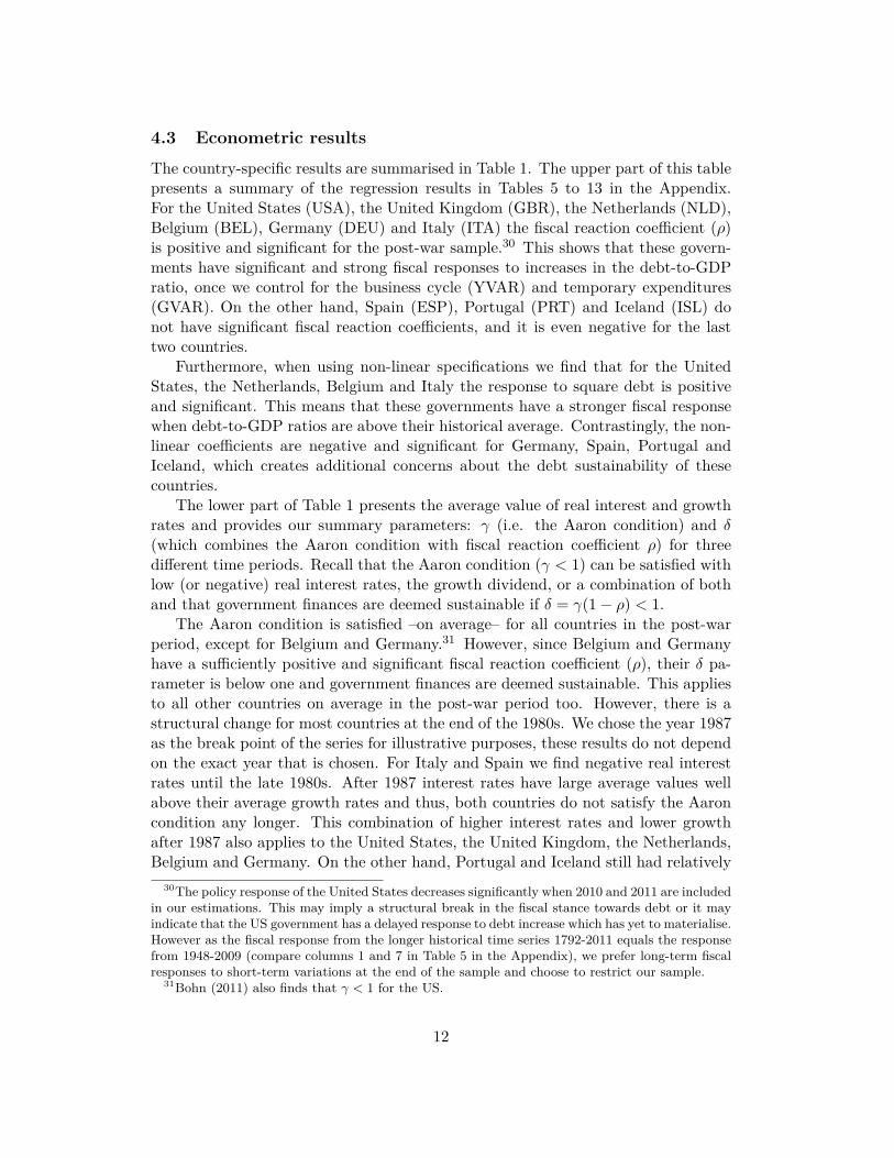
4.3 Econometric results

The country-specific results are summarised in Table 1. The upper part of this tablepresents a summary of the regression results in Tables 5 to 13 in the Appendix.For the United States (USA), the United Kingdom (GBR), the Netherlands (NLD),Belgium (BEL), Germany (DEU) and Italy (ITA) the fiscal reaction coefficient (𝜌)is positive and significant for the post-war sample.30 This shows that these govern-ments have significant and strong fiscal responses to increases in the debt-to-GDPratio, once we control for the business cycle (YVAR) and temporary expenditures(GVAR). On the other hand, Spain (ESP), Portugal (PRT) and Iceland (ISL) donot have significant fiscal reaction coefficients, and it is even negative for the lasttwo countries.

Furthermore, when using non-linear specifications we find that for the UnitedStates, the Netherlands, Belgium and Italy the response to square debt is positiveand significant. This means that these governments have a stronger fiscal responsewhen debt-to-GDP ratios are above their historical average. Contrastingly, the non-linear coefficients are negative and significant for Germany, Spain, Portugal andIceland, which creates additional concerns about the debt sustainability of thesecountries.

The lower part of Table 1 presents the average value of real interest and growthrates and provides our summary parameters: 𝛾 (i.e. the Aaron condition) and 𝛿(which combines the Aaron condition with fiscal reaction coefficient 𝜌) for threedifferent time periods. Recall that the Aaron condition (𝛾 < 1) can be satisfied withlow (or negative) real interest rates, the growth dividend, or a combination of bothand that government finances are deemed sustainable if 𝛿 = 𝛾(1 − 𝜌) < 1.

The Aaron condition is satisfied –on average– for all countries in the post-warperiod, except for Belgium and Germany.31 However, since Belgium and Germanyhave a sufficiently positive and significant fiscal reaction coefficient (𝜌), their 𝛿 pa-rameter is below one and government finances are deemed sustainable. This appliesto all other countries on average in the post-war period too. However, there is astructural change for most countries at the end of the 1980s. We chose the year 1987as the break point of the series for illustrative purposes, these results do not dependon the exact year that is chosen. For Italy and Spain we find negative real interestrates until the late 1980s. After 1987 interest rates have large average values wellabove their average growth rates and thus, both countries do not satisfy the Aaroncondition any longer. This combination of higher interest rates and lower growthafter 1987 also applies to the United States, the United Kingdom, the Netherlands,Belgium and Germany. On the other hand, Portugal and Iceland still had relatively

30The policy response of the United States decreases significantly when 2010 and 2011 are includedin our estimations. This may imply a structural break in the fiscal stance towards debt or it mayindicate that the US government has a delayed response to debt increase which has yet to materialise.However as the fiscal response from the longer historical time series 1792-2011 equals the responsefrom 1948-2009 (compare columns 1 and 7 in Table 5 in the Appendix), we prefer long-term fiscalresponses to short-term variations at the end of the sample and choose to restrict our sample.

31Bohn (2011) also finds that 𝛾 < 1 for the US.

12

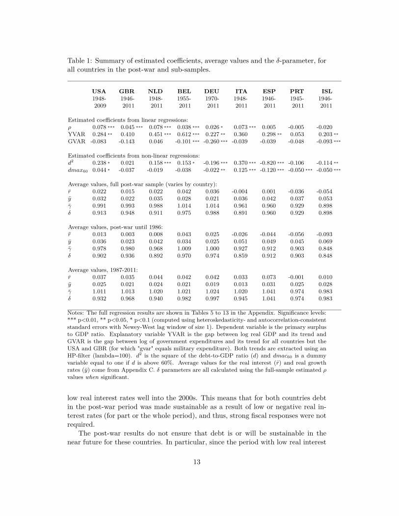
Table 1: Summary of estimated coefficients, average values and the 𝛿-parameter, forall countries in the post-war and sub-samples.

USA GBR NLD BEL DEU ITA ESP PRT ISL1948-2009

1946-2011

1948-2011

1955-2011

1970-2011

1948-2011

1946-2011

1945-2011

1946-2011

Estimated coefficients from linear regressions:𝜌 0.078 *** 0.045 *** 0.078 *** 0.038 *** 0.026 * 0.073 *** 0.005 -0.005 -0.020YVAR 0.284 ** 0.410 0.451 *** 0.612 *** 0.227 ** 0.360 0.298 ** 0.053 0.203 **

GVAR -0.083 -0.143 0.046 -0.101 *** -0.260 *** -0.039 -0.039 -0.048 -0.093 ***

Estimated coefficients from non-linear regressions:𝑑2 0.238 * 0.021 0.158 *** 0.153 * -0.196 *** 0.370 *** -0.820 *** -0.106 -0.114 **

𝑑𝑚𝑎𝑥60 0.044 * -0.037 -0.019 -0.038 -0.022 ** 0.125 *** -0.120 *** -0.050 *** -0.050 ***

Average values, full post-war sample (varies by country):𝑟 0.022 0.015 0.022 0.042 0.036 -0.004 0.001 -0.036 -0.054𝑦 0.032 0.022 0.035 0.028 0.021 0.036 0.042 0.037 0.053𝛾 0.991 0.993 0.988 1.014 1.014 0.961 0.960 0.929 0.898𝛿 0.913 0.948 0.911 0.975 0.988 0.891 0.960 0.929 0.898

Average values, post-war until 1986:𝑟 0.013 0.003 0.008 0.043 0.025 -0.026 -0.044 -0.056 -0.093𝑦 0.036 0.023 0.042 0.034 0.025 0.051 0.049 0.045 0.069𝛾 0.978 0.980 0.968 1.009 1.000 0.927 0.912 0.903 0.848𝛿 0.902 0.936 0.892 0.970 0.974 0.859 0.912 0.903 0.848

Average values, 1987-2011:𝑟 0.037 0.035 0.044 0.042 0.042 0.033 0.073 -0.001 0.010𝑦 0.025 0.021 0.024 0.021 0.019 0.013 0.031 0.025 0.028𝛾 1.011 1.013 1.020 1.021 1.024 1.020 1.041 0.974 0.983𝛿 0.932 0.968 0.940 0.982 0.997 0.945 1.041 0.974 0.983

Notes: The full regression results are shown in Tables 5 to 13 in the Appendix. Significance levels:*** p<0.01, ** p<0.05, * p<0.1 (computed using heteroskedasticity- and autocorrelation-consistentstandard errors with Newey-West lag window of size 1). Dependent variable is the primary surplusto GDP ratio. Explanatory variable YVAR is the gap between log real GDP and its trend andGVAR is the gap between log of government expenditures and its trend for all countries but theUSA and GBR (for which "gvar" equals military expenditure). Both trends are extracted using anHP-filter (lambda=100). 𝑑2 is the square of the debt-to-GDP ratio (𝑑) and 𝑑𝑚𝑎𝑐60 is a dummyvariable equal to one if 𝑑 is above 60%. Average values for the real interest (𝑟) and real growthrates (𝑦) come from Appendix C. 𝛿 parameters are all calculated using the full-sample estimated 𝜌values when significant.

low real interest rates well into the 2000s. This means that for both countries debtin the post-war period was made sustainable as a result of low or negative real in-terest rates (for part or the whole period), and thus, strong fiscal responses were notrequired.

The post-war results do not ensure that debt is or will be sustainable in thenear future for these countries. In particular, since the period with low real interest

13

rates ended, the importance of fiscal responses has greatly increased. Countriesthat lack a significant fiscal response may then have difficulties to maintain debt-to-GDP ratios at sustainable levels. Moreover, the absence of a linear fiscal response,in conjunction with a negative non-linear response for Germany, Spain, Portugaland Iceland rises the concern that debt may not be sustainable in these countries.Our stochastic analysis in Section 6 will use this information combined with a VARanalysis to provide our early-warning sustainability indicator.

4.4 Sensitivity analysis

In this section we test the robustness of our econometric results and present theoutcomes per country in Tables 5 to 13 in the Appendix.

First, we employ alternative definitions of GVAR, for some countries, and YVARfor all countries. For the United States and the United Kingdom –where militaryspending has been historically a big driver of temporary government spending– wedefine GVAR as the military spending-to-GDP ratio.32 For the Netherlands we usegas revenue as a proxy for GVAR following Wierts and Schotten (2008). Moreover,we run the regressions without any GVAR term (only YVAR) and the estimated𝜌 values remain significant (with the exception of Germany) and with qualitativelysimilar values. For YVAR we employ instead of the difference of actual real GDPfrom a trend extracted by an HP-filter the difference of actual real GDP from amoving average of 8 years, where assess a mid-point moving average, which uses3 years prior to the current year, the current year and four years after, and anend-point moving average, which uses the previous 8 years and corrects for averagegrowth. In the last case the fiscal response increases significantly for Belgium andItaly.

Second, we include the real interest rate as an explanatory variable in equation(2). The intuition is that the primary surplus can also react to changes in real interestrates. For instance, when governmental policies generate negative real interest rates(e.g. through financial repression) the government faces less pressure to reduce thedebt with fiscal responses. Also, high real interest rates can force the governmentto apply fiscal austerity, even when the debt-to-GDP level is not that high. For theUnited States, Bohn (1998) found that interest rates are not a significant controlvariable. We find similar results for all countries but Germany, where the inclusion ofthe real interest rates yields a non-significant 𝜌 parameter. We also include inflationas an additional variable as high inflation allows for a less responsive fiscal policy.Inflation turns out to be insignificant in most cases, and when it is significant it doesnot change the fiscal response parameter.

Third, we assess the stability of the fiscal response over time. The most obviouschoice is to include the full historical sample available and not only the post-war

32This is comparable to Bohn (2008) who defines GVAR as the gap between a permanent com-ponent of military outlays to GDP from an estimated AR(2) process and the actual values. Ourapproach probably overestimates temporary military spending by a constant term, which likely hasno impact on our estimate of 𝜌.

14

period. These results are presented in the penultimate column of the country-specificTables in Appendix B –except for Germany for which we do not have data before1970. It is remarkable that for the United States and the United Kingdom, the full-sample historical fiscal reaction coefficient is significant and very close in value to thepost-war estimation. For the Netherlands and Belgium the full-sample coefficientis significant but has a lower value. While for Italy and Spain the significance ofthe coefficients for both samples is reversed. In Italy 𝜌 is significant in the post-warsample, but it is not significant in the full-sample, while in Spain only the historical𝜌 coefficient is significant. Portugal and Iceland have non-significant coefficientsfor both samples. We also used Bai and Perron (1998, 2003) tests for endogenousstructural breaks after the Second World War. The resulting sub-samples, however,are usually too short to estimate a stable fiscal reaction function that can assessthe long-run institutional stance towards fiscal sustainability.33 In that case 𝜌 picksup short-term policy fluctuations and is not suitable for our analysis. The samelogic applies when dropping an arbitrary post-war sub-sample. In developing ourearly-warning indicator we estimated our FRF for a post-war sample that ends in2007, instead of 2011. This specification intends to eliminate the possible effects ofthe current financial crisis on our estimations. We find that for only three countriesthe significance of the 𝜌 parameter is changed: Spain has now a highly significant(𝑝 < 0.01) coefficient of 0.07, Portugal has a lower significant (𝑝 < 0.1) coefficient of0.02, and the significance level of the German coefficient is increased.

Fourth, to assess the impact of potential codeterminacy of the response of pri-mary surplus to debt, the business cycle and temporary government spending, weperform two checks: we use one-year lagged variables for YVAR and GVAR andwe estimate our regression with GMM with lags of debt, YVAR, GVAR, primarysurplus, inflation, real growth rates and real interest rates as instruments. We findthat the 𝜌 coefficient remains robust to this specification. In general, we find itreasonable to expect that the business cycle will be independent of country-specificdebt level.34 In the case of temporary government expenditures, when they are prox-ied by military expenditure –as in the original FRF estimations for the US by Bohn(1998, 2008)– we also find it reasonable to assume that these are independent of debtlevels. When GVAR is estimated as the cyclical component of government expendi-ture, the case is less compelling. However, as explained above, the use of GVAR asan independent variable is not critical to our estimations of the 𝜌 coefficient.

Fifth, we check whether there is a delay in the response of fiscal policy to debtmight have a downward bias on our fiscal response functions by including laggedprimary surplus. The total effect is than the coefficient of the response of debtdivided by one minus the coefficient of lagged primary surplus. The results are very

33In addition, these shorter samples are sensitive to specific political events that affected govern-ment behaviour in the period. For instance, the dictatorship years in Spain and Portugal underFranco and Salazar.

34Note that this does not mean that in short-term (year-to-year) episodes there might be a causalinterplay between both variables. But in our historical long-term analysis we do not expect suchan interaction to be problematic.

15

similar. This can be explained by the fact that the debt ratio is a slow movingvariable, which means that the effect of an increase in the debt ratio will persistover time even if the response of primary surplus is small initially. Thus, as in Bohn(1998, 2008) we find that OLS estimations of the FRF is a reasonable approach.

5 Stochastic debt sustainability simulationsThe results presented in the previous section are based on the assumption thatinterest and growth rates are equal to their long-run average. However, interest andgrowth rates fluctuate over time and this has a significant impact on the evolution ofthe debt level. Higher interest and growth rate volatility increases the distribution offuture debt levels and requires a larger fiscal response to keep government debt undercontrol. For instance, Catão and Kapur (2006) provide evidence that differences inmacroeconomic volatility are the key determinant of higher spreads.35

To assess this relationship we extend the results from the previous section bysimulating future interest and growth rate values, which in turn provide a probabilitydistribution for future debt-to-GDP levels.

Specifically, we insert simulated interest and growth rates, represented by 𝛾𝑡,into equation (3):

𝑑𝑡+1 = 𝛾𝑡(1 − 𝜌)𝑑𝑡 − 𝛾𝑡𝛼. (5)

Here we used that by construction 𝐸(Zt) = 0 and 𝐸(𝜀𝑡) = 0. To obtain a path forthe public debt level 𝑑𝑡, we integrate forward equation (5).36 The simulated interestand growth rates of every step are obtained from a simple two variable VAR modelfollowing Budina and van Wijnbergen (2008). This VAR model captures the historicvolatility of interest and growth rates:(︃

𝑟𝑡

𝑦𝑡

)︃= 𝛼0 +

𝑇∑︁𝑗=1

𝐴𝑗

(︃𝑟𝑡−𝑗

𝑦𝑡−𝑗

)︃+ 𝜂𝑡, (6)

var (𝜂𝑡) = V

In this set-up shocks to real interest and growth rates are not correlated over time butare correlated within the same time period. The interest and growth rate themselvesare correlated over time and within the same time period due to the auto-regressivespecification.

We then run this procedure ten thousand times to obtain a distribution of futuredebt paths. The set of debt levels from the simulation at time 𝑡 + 𝑠 is then the dis-tribution of expected future debt levels at time 𝑡 + 𝑠. The shape of the distribution

35In a related study, Genberg and Sulstarova (2008) show how the right hand tail of the distribu-tion of the debt-to-GDP ratio depends on the second moments (i.e. variability) of macroeconomicvariables and then regresses these second moments on interest spreads.

36To get debt at time 𝑡 + 1 –i.e. 𝑑𝑡+1– we substitute 𝑑𝑡 and the interest and growth rates ofperiod 𝑡 in equation (5). Then, to get 𝑑𝑡+2, we use the estimated 𝑑𝑡+1 and the interest and growthrates in period 𝑡 + 1 and so on and so forth.

16

of debt paths is informative on fiscal sustainability. In particular, a narrower distri-bution indicates greater certainty on future debt levels and characterises a countrythat is more in control of its finances.

Two main processes influence this distribution. First, higher volatility in interestand growth rates broadens the distribution of future debt levels. Second, a largerfiscal response narrows the distribution. This latter happens because, for 𝜌 > 0,fiscal policy responds to a deviation in the debt level from its steady state value𝑑. Then, shocks in interest and growth rates that drive the debt level away from𝑑 are countered by a fiscal response in the subsequent period(s). Similarly, shocksthat drive the debt level towards 𝑑 are mitigated by a smaller fiscal response. Thiseffect is stronger for larger 𝜌. Furthermore, if the fiscal response is too weak or ifthe volatility of interest and growth rates is too strong, the width of the distributionmay grow without bound over time. In this case the distribution is not properlydefined (i.e. bounded) and, as Hall (2013) shows, the debt level is not stationary.

Our simulations generate a debt path for the period: 2012-2021. We run thesimulation for two scenarios: one with the estimated 𝜌 values (cf. Table 1) andanother where we assume no fiscal response, i.e. 𝜌 = 0.37 Equation (6) is estimatedper country using 1987 as a starting point. We thus do not use the historically lowreal interest rates period experienced in the preceding decades. In addition, we setthe number of lags equal to two in equation (6).38

The simulated distributions of expected future debt levels are shown in Figures2 to 4. Note that the left-hand figure always includes a fiscal response (𝜌 > 0).This implies that for those countries with 𝜌 = 0: Spain, Portugal and Iceland, weartificially set 𝜌 = 7% for illustrative purposes. All right-hand figures have 𝜌 = 0.The debt level is on the vertical axes and time is on the horizontal axis. The blackline indicates the median debt level from the simulated distribution, the light orangearea contains 90% of the simulation results and the dark orange area contains thenext 5%. The two blue lines are visual aids at the 60% and the 90% debt level.

In general, the width of the simulated debt distributions is determined by thevariability of the growth and interest rates, while the fiscal reaction (𝜌) affects themedian of the distribution –although it also has a slightly effect on the width of thedistribution.

The debt levels have relatively small 90% and 95% confidence bands for thefirst set of countries: the United States, United Kingdom, Netherlands, Belgiumand Germany. For the second group –Italy, Spain, Portugal and Iceland– theseconfidence bands are larger, due to the larger variability in growth and interest

37For 𝜌 = 0 we use 𝛼 = ps in equation (5), with ps the average primary surplus. This correctionprevents a change in the average fiscal stance while making fiscal policy irresponsive to the debtlevel.

38Given the number of observations, we could use one or two lags. We test for the number of lagsto include using the Akaike Information Criterion. The differences are small and we chose two forall countries as it allows for richer dynamics. The Cholesky-decomposed covariance matrix of theresiduals is given in Table 4. We have tested for autocorrelation in the residuals and were able toreject and tested for stability of the VAR and found that for most countries all eigenvalues are inthe unit circle.

17

rates experienced by these countries. From Figures 3 and 4 it is clear that theimposed value of 𝜌 = 7% is not sufficiently large for Italy, Spain or Portugal to bringthe bandwidth of simulations results to levels comparable with the other countries.

For 𝜌 = 0 we see that the median debt levels are higher when there is no fiscalresponse.39 Furthermore, the width of the distribution slightly increases vis-à-vis𝜌 > 0 for all countries. On the other hand, Portugal still has a very explosivedebt path even with a positive fiscal reaction coefficient of 𝜌 = 7%. This is due tothe large historical Portuguese volatility over real growth and interest rates, whichcreates large uncertainties and wide confidence bands in our simulations.

Figure 2: Stochastic debt projections for the United States, from 2011 to 2021. 𝜌denotes the fiscal response.

90%

120%

150% United States, ρ=7.8%

0%

30%

60%

2011 2016 2021

90%

120%

150% United States, ρ=0

0%

30%

60%

2011 2016 2021

Notes: The dark orange band with p<0.95 encompasses also the light orange band with p<0.90.

39The Netherlands and Belgium are the exception, because both countries are characterised bya strong fiscal response and a relatively stable debt level (see Figure 1). The fiscal response reactsto both increases and reductions of the debt level from its long-run average, but in the Dutch andBelgian case the latter applies. For instance, the inclusion of the fiscal response "stabilises" theDutch debt level around its post-war average of 60%, and this results in the projected median debtlevel being lower with 𝜌 = 0 than with 𝜌 > 0.

18

Figure 3: Stochastic debt projections for the United Kingdom, the Netherlands,Belgium and Germany from 2011 to 2021. 𝜌 denotes the fiscal response.

90%

120%

150% United Kingdom, ρ=4.5%

0%

30%

60%

2011 2016 2021

90%

120%

150% United Kingdom, ρ=0

0%

30%

60%

2011 2016 2021

90%

120%

150% Netherlands, ρ=7.7%

0%

30%

60%

2011 2016 2021

90%

120%

150% Netherlands, ρ=0

0%

30%

60%

2011 2016 2021

90%

120%

150% Belgium, ρ=3.8%

0%

30%

60%

2011 2016 2021

90%

120%

150% Belgium, ρ=0

0%

30%

60%

2011 2016 2021

90%

120%

150% Germany, ρ=2.6%

0%

30%

60%

2011 2016 2021

90%

120%

150% Germany, ρ=0

0%

30%

60%

2011 2016 2021

Notes: The dark orange band with p<0.95 encompasses also the light orange band with p<0.90.

19

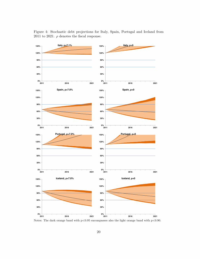
Figure 4: Stochastic debt projections for Italy, Spain, Portugal and Iceland from2011 to 2021. 𝜌 denotes the fiscal response.

90%

120%

150% Italy, ρ=7.1%

0%

30%

60%

2011 2016 2021

90%

120%

150% Italy, ρ=0

0%

30%

60%

2011 2016 2021

90%

120%

150% Spain, ρ=7.0%

0%

30%

60%

2011 2016 2021

90%

120%

150% Spain, ρ=0

0%

30%

60%

2011 2016 2021

90%

120%

150% Portugal, ρ=7.0%

0%

30%

60%

2011 2016 2021

90%

120%

150% Portugal, ρ=0

0%

30%

60%

2011 2016 2021

90%

120%

150% Iceland, ρ=7.0%

0%

30%

60%

2011 2016 2021

90%

120%

150% Iceland, ρ=0

0%

30%

60%

2011 2016 2021

Notes: The dark orange band with p<0.95 encompasses also the light orange band with p<0.90.

20

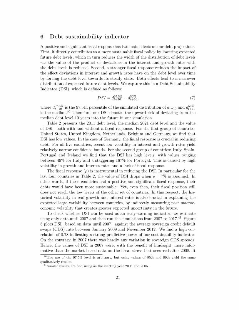
6 Debt sustainability indicatorA positive and significant fiscal response has two main effects on our debt projections.First, it directly contributes to a more sustainable fiscal policy by lowering expectedfuture debt levels, which in turn reduces the width of the distribution of debt levels–as the value of the product of deviations in the interest and growth rates withthe debt levels is reduced. Second, a stronger fiscal response reduces the impact ofthe effect deviations in interest and growth rates have on the debt level over timeby forcing the debt level towards its steady state. Both effects lead to a narrowerdistribution of expected future debt levels. We capture this in a Debt SustainabilityIndicator (DSI), which is defined as follows:

𝐷𝑆𝐼 = 𝑑97.5%𝑡+10 − 𝑑50%

𝑡+10, (7)

where 𝑑97.5%𝑡+10 is the 97.5th percentile of the simulated distribution of 𝑑𝑡+10 and 𝑑50%

𝑡+10is the median.40 Therefore, our DSI denotes the upward risk of deviating from themedian debt level 10 years into the future in our simulation.

Table 2 presents the 2011 debt level, the median 2021 debt level and the valueof DSI –both with and without a fiscal response. For the first group of countries:United States, United Kingdom, Netherlands, Belgium and Germany, we find thatDSI has low values. In the case of Germany, the fiscal response is crucial in reducingdebt. For all five countries, recent low volatility in interest and growth rates yieldrelatively narrow confidence bands. For the second group of countries: Italy, Spain,Portugal and Iceland we find that the DSI has high levels, with values rangingbetween 49% for Italy and a staggering 167% for Portugal. This is caused by highvolatility in growth and interest rates and a lack of fiscal response.

The fiscal response (𝜌) is instrumental in reducing the DSI. In particular for thelast four countries in Table 2, the value of DSI drops when 𝜌 = 7% is assumed. Inother words, if these countries had a positive and significant fiscal response, theirdebts would have been more sustainable. Yet, even then, their fiscal position stilldoes not reach the low levels of the other set of countries. In this respect, the his-torical volatility in real growth and interest rates is also crucial in explaining theexpected large variability between countries, by indirectly measuring past macroe-conomic volatility that creates greater expected uncertainty in the future.

To check whether DSI can be used as an early-warning indicator, we estimateusing only data until 2007 and then run the simulations from 2007 to 2017.41 Figure5 plots DSI –based on data until 2007– against the average sovereign credit defaultswaps (CDS) rate between January 2009 and November 2012. We find a high cor-relation of 0.78 indicating a strong predictive power of our sustainability indicator.On the contrary, in 2007 there was hardly any variation in sovereign CDS spreads.Hence, the values of DSI in 2007 were, with the benefit of hindsight, more infor-mative than the market based data on the fiscal stress that occurred after 2008. It

40The use of the 97.5% level is arbitrary, but using values of 95% and 99% yield the samequalitatively results.

41Similar results are find using as the starting year 2006 and 2005.

21

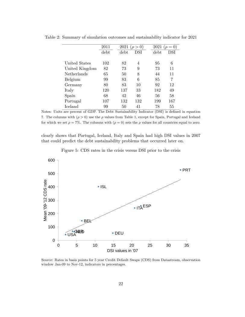
Table 2: Summary of simulation outcomes and sustainability indicator for 2021

2011 2021 (𝜌 > 0) 2021 (𝜌 = 0)debt debt DSI debt DSI

United States 102 82 4 95 6United Kingdom 82 73 9 73 11Netherlands 65 50 8 44 11Belgium 99 83 6 85 7Germany 80 83 10 92 12Italy 120 137 33 182 49Spain 68 42 46 56 58Portugal 107 132 132 199 167Iceland 99 50 41 78 55

Notes: Units are percent of GDP. The Debt Sustainability Indicator (DSI) is defined in equation7. The columns with (𝜌 > 0) use the 𝜌 values from Table 1, except for Spain, Portugal and Icelandfor which we set 𝜌 = 7%. The columns with (𝜌 = 0) sets the 𝜌 values for all countries equal to zero.

clearly shows that Portugal, Iceland, Italy and Spain had high DSI values in 2007that could predict the debt sustainability problems that occurred later on.

Figure 5: CDS rates in the crisis versus DSI prior to the crisis

USA GBR NLD

BEL

DEU

ITA ESP

PRT

ISL

0

100

200

300

400

500

600

0 5 10 15 20 25 30 35

Mean

'09-'12

CD

S r

ate

DSI values in '07

Source: Rates in basis points for 5 year Credit Default Swaps (CDS) from Datastream, observationwindow Jan-09 to Nov-12, indicators in percentages.

22

While these results support using DSI as an early-warning instrument, a morerigorous assessment with a wider sample of countries that employs the signals ap-proach of Kaminsky et al. (1998) should be undertaken.42 Kaminsky et al. (1998)proposes, in the context of currency crisis, an early warning system based on thesignal-to-noise ratio of an indicator for predicting a crisis.43

7 Summary and conclusionsWe develop an indicator for debt sustainability which measures upward risk. Itcombines the effect of economic uncertainty –captured by stochastic simulations ofinterest and growth rates– with the expected response of the government budgetto the debt level. We use long time series and find that five countries: the UnitedStates, United Kingdom, Netherlands, Belgium and Germany have persistently posi-tive and significant fiscal reaction coefficients, conditional on temporary governmentspending (e.g. war expenditure) and cyclical economic fluctuations. These strongfiscal responses are found in both the full sample and also in the post-war period. Inconjunction with on average moderate real growth and interest rates, their debt-to-GDP ratios have been sustainable over time. Except for Germany, these countriesemerged from the Second World War with high debt-to-GDP ratios. Until the mid-seventies, these debt levels were reduced drastically through low real interest rates.After the mid-seventies, real interest rates increased, while real growth rates werereduced and thus, these countries relied increasingly on fiscal responsibility (i.e.moderate primary surplus to GDP ratios) to keep debt at sustainable levels. Thelow values of our estimated DSI correctly reflect these facts.

On the other hand, for Spain, Portugal and Iceland, we do not find a significantfiscal response. Therefore, if real interest rates increase these countries are lessprepared to maintain sustainable debt levels in the future. Our DSI clearly identifiesthis weakness in the debt dynamics of these countries by showing large upward risk.Finally, Italy has a positive and significant fiscal response coefficient, yet has debtsustainability concerns as its high current debt level makes it very susceptible tofluctuations in interest and growth rates. Therefore its debt sustainability indicatoris large, which justifies the doubts on Italy’s debt sustainability. As an aside, notethat from a pure modelling point of view a better debt sustainability indicator for

42As a complement to this paper, we are currently expanding the country sample to includeadditional OECD countries and also emerging economies.

43This approach does not attempt to explain what drives the default probability, but merelytries to make a predictor that is as accurate as possible. Related papers include Berg et al. (2005)who perform a review of early-warning systems focusing primarily on the 1997 Asian crisis andreport mixed results. Over the global financial crisis, Shi and Gao (2010) show the Kaminsky et al.(1998) early warning system did reasonably well during the crisis, albeit in a modified form. Severalextensions to these type of indicators have recently been made. Dobrescu et al. (2011) extend theanalysis to near-default events and show that including near-default events shows that fiscal stressremains high in advanced economies. Ciarlone and Trebeschi (2005) extend the two-state approach(default, non-default) to a three-state (default, non-default and post-default) and generate an earlywarning system which predicts 76% of entries into crisis, with 36% false alarms.

23

Italy is more readily obtained by having a lower initial debt level and/or lowervolatility in interest and growth rates than by increasing its fiscal response,whichare similar to those in the United States, United Kingdom, Netherlands, Belgiumand Germany, by strengthening fiscal institutions.

For medium to long-term fiscal policy assessments, indicators based on stochasticanalysis and expected fiscal responses have several advantages over the currentlyavailable indicators at a medium term horizon. Both the momentary indicators (debtand deficit levels) and the ageing indicators (S1, S2) are static and do not capturevolatility in the economy and the government’s ability to control public finances.Alternative indicators currently in use, such as structural balances or cyclicallyadjusted budget balances (CABB), are often plagued by measurement issues. Theydepend on projections of future growth, which are known to have an upward bias(Larch and Salto, 2005), and their estimates are vulnerable to endogeneity problems:it is non-trivial to disentangle the effects of expected growth on the CABB fromthe effects the CABB has on expected growth. Our indicator do not suffer fromthese shortcomings, since it incorporates economic volatility and the government’sexpected policy response from ex-post realisations only.

Our analysis, however, has some caveats. First, our estimated fiscal response (𝜌)is an institutional variable that measures how - over medium and long-time periods –the government of a particular country deals with medium/long term changes in debtlevels. This means that we require long time series to estimate 𝜌, and furthermore,our approach is not suitable to analyse short-term debt sustainability. It cannotprovide information on whether -for example- Spain will be able to roll over itsdebt in the coming months. Second, the shocks in our simulations depend on thehistoric volatility of interest and growth rates. That means they do not containall possible unexpected exogenous events (e.g. war, natural disasters). The resultsof our simulation exercise are not informative on debt sustainability under suchcatastrophic conditions. Third, our indicator is not informative on the policy changethat will solve the debt sustainability issue. Our framework merely states thatcountries with a higher and more significant historical fiscal policy response aremore likely to solve such issues, should they arise.44

Therefore, our indicator is not meant to replace current indicators, but ratherto complement the short term indicators and the indicators from ageing studies.They could, for instance, provide guidance on whether it is reasonable for a countryto join a monetary union. In such a union, the use of financial and monetarypolicies is limited for individual countries, making it unlikely for them to achieve debtreductions through policies that yield very low or negative real interest rates. Thus,there is an increased dependence on fiscal policy to tackle debt sustainability. Ourindicator captures this medium- to long-term institutional relation between fiscalpolicy and debt sustainability and complements it with the historical macroeconomic

44In contrast, ageing studies (European Commission, 2012a) analyse the impact of ageing onpublic finances given constant policy arrangements. If public finances are unsustainable, the policyarrangements most impacted by ageing should change until the problem is alleviated.

24

stability of each country that is implicit in the volatility of real growth and interestrates.

Finally, we show that our indicator can be potentially useful as an early-warningindicator for debt sustainability, as it would have provided valuable information backin 2007 regarding the European sovereign debt crisis. Further tests, however, arestill necessary to check the sensitivity of the DSI to different countries and samples,and to have a more robust assessment on how DSI performs as an early-warningdebt sustainability indicator.

25

ReferencesAaron, H. (1966). “The Social Insurance Paradox,” Canadian Journal of Economics

and Political Science, 32(3), 371–374.

Afonso, A. (2005). “Fiscal Sustainability: The Unpleasant European Case,” Finan-zArchiv, 61(1), 19–44.

Arezki, R., B. Candelon, and A. Sy (2011). “Sovereign Rating News and Finan-cial Markets Spillovers: Evidence from the European Debt Crisis,” IMF WorkingPaper 11/69.

Baffigi, A. (2011). “Italian National Accounts, 1861-2011,” Economic History Work-ing Papers 18, Banca d’Italia.

Bai, J. and P. Perron (1998). “Estimating and Testing Linear Models with MultipleStructural Changes,” Econometrica, 66(1), 47–78.

Bai, J. and P. Perron (2003). “Computation and Analysis of Multiple StructuralChange Models,” Journal of Applied Econometrics, 18(1), 1–22.

Barro, R. J. (1979). “On the Determination of Public Debt,” Journal of PoliticalEconomy, 87(5), 940–971.

Bartoletto, S., B. Chiarini, and E. Marzano (2013). “Is the Italian Public DebtReally Unsustainable? An Historical Comparison (1861-2010),” CESifo WorkingPaper Series 4185.

Baum, A., C. Checherita-Westphal, and P. Rother (2013). “Debt and Growth: NewEvidence for the Euro Area,” Journal of International Money and Finance, 32,809–821.

Beetsma, R. and M. Giuliodori (2010). “The Macroeconomic Costs and Benefits ofthe EMU and Other Monetary Unions: An Overview of Recent Research,” Journalof Economic Literature, 48(3), 603–641.

Berg, A., E. Borensztein, and C. Pattillo (2005). “Assessing Early Warning Systems:How Have They Worked in Practice?” IMF Staff Papers, 52(3), 462–502.

Berti, K. (2013). “Stochastic Public Debt Projections Using the Historical Variance-Covariance Matrix Approach for EU Countries,” European Economy - EconomicPapers 480, Directorate General Economic and Monetary Affairs (DG ECFIN),European Commission.

Berti, K., M. Salto, and M. Lequien (2012). “An Early-detection Index of FiscalStress for EU Countries,” European Economy - Economic Papers 475, DirectorateGeneral Economic and Monetary Affairs (DG ECFIN), European Commission.

26

Bohn, H. (1991). “Budget Balance Through Revenue or Spending Adjustments?Some Historical Evidence for the United States,” Journal of Monetary Economics,27(3), 333–359.

Bohn, H. (1998). “The Behavior of U.S. Public Debt and Deficits,” Quarterly Journalof Economics, 113(3), 949–963.

Bohn, H. (2007). “Are Stationary and Cointegration Restrictions Really Neces-sary for the IntertemporalBudget Constraing?” Journal of Monetary Economics,54(7), 1837–1847.

Bohn, H. (2008). “The Sustainability of Fiscal Policy in the United States,” inSustainability of Public Debt, ed. by R. Neck and J. Sturm, MIT Press, 15–49.

Bohn, H. (2011). “The Economic Consequences of Rising U.S. Government Debt:Privileges at Risk,” FinanzArchiv: Public Finance Analysis, 67(3), 282–302.

Bos, F. (2007). “The Dutch Fiscal Framework: History, Current Practice and theRole of the CPB,” CPB Discussion Paper, 150.

Brender, A. and A. Drazen (2005). “Political Budget Cycles in New Versus Estab-lished Democracies,” Journal of Monetary Economics, 52(7), 1271–1295.

Brender, A. and A. Drazen (2008). “How Do Budget Deficits and Economic GrowthAffect Reelection Prospects? Evidence from a Large Panel of Countries,” Ameri-can Economic Review, 98(5), 2203–20.

Budina, N. and S. van Wijnbergen (2008). “Quantitative Approaches to Fiscal Sus-tainability Analysis: A Case Study of Turkey since the Crisis of 2001,” WorldBank Economic Review, 23(1), 119–140.

Bursian, D., A. J. Weichenrieder, and J. Zimmer (2015). “Trust in Government andFiscal Adjustments,” International Tax and Public Finance, 22(4), 663–682.

Callen, T., M. Terrones, X. Debrun, J. Daniel, and C. Allard (2003). “Public Debtin Emerging Markets: Is it Too High?” in World Economic Outlook, InternationalMonetary Fund, chap. III.

Catão, L. and S. Kapur (2006). “Volatility and the Debt-Intolerance Paradox,” IMFStaff Papers, 53(2), 195–218.

CBS (1959). “Zestig jaren statistiek in tijdreeksen (1899-1959),” .

CBS (1994). “Vijfennegentig jaren statistiek in tijdreeksen (1899-1994),” .

CBS (2001). “Tweehonderd jaar statistiek in tijdreeksen (1800-1999),” .

Cecchetti, S., M. Mohanty, and F. Zampolli (2011). “The Real Effects of Debt,” BISWorking Papers 352, Bank for International Settlements.

27

Celasun, O., X. Debrun, and J. D. Ostry (2006). “Primary Surplus Behavior andRisks to Fiscal Sustainability in Emerging Market Countries: A "Fan-Chart" Ap-proach,” IMF Working Papers 06/67, International Monetary Fund.

Checherita-Westphal, C. and P. Rother (2012). “The Impact of High GovernmentDebt on Economic Growth and its Channels: An Empirical Investigation for theEuro Area,” European Economic Review, 56(7), 1392–1405.

Ciarlone, A. and G. Trebeschi (2005). “Designing an Early Warning System for DebtCrises,” Emerging Markets Review, 6(4), 376–395.

Comín, F. and D. Díaz (2005). “Sector Público Administrativo y Estado del Bienes-tar,” in Estadísticas Históricas de España: Siglos XIX y XX, ed. by A. Carrerasand X. Tafunell, Bilbao, Spain: Fundación BBVA, 873–964, 2nd edition ed.

Dobrescu, G., I. Petrova, N. Belhocine, and E. Baldacci (2011). “Assessing FiscalStress,” IMF Working Papers 11/100, International Monetary Fund.

Égert, B. (2012). “Public Debt, Economic Growth and Nonlinear Effects: Myth orReality?” OECD Economics Department Working Papers 993, OECD Publishing.

European Commission (2012a). “Fiscal Sustainability Report 2012,” EuropeanEconomy 8/2012, Directorate-General for Economic and Financial Affairs, Brus-sels.

European Commission (2012b). “Report on Public Finances in the EMU,” Euro-pean Economy 4/2012, Directorate-General for Economic and Financial Affairs,Brussels.

Genberg, H. and A. Sulstarova (2008). “Macroeconomic Volatility, Debt Dynam-ics, and Sovereign Interest Rate Spreads,” Journal of International Money andFinance, 27(1), 26–39.

Ghosh, A. R., J. I. Kim, E. G. Mendoza, J. D. Ostry, and M. S. Qureshi (2013).“Fiscal Fatigue, Fiscal Space and Debt Sustainability in Advanced Economies,”The Economic Journal, 123(566), F4–F30.

Hall, R. E. (2013). “Fiscal Stability of High-Debt Nations under Volatile EconomicConditions,” Working Paper 18797, National Bureau of Economic Research.

Höppner, F. and C. Kastrop (2004). “Fiscal Institutions and Sustainability of PublicDebt in Germany,” in Banca d’Italia Workshop on Public Debt, Perugia, Italia:Banca d’Italia, 575–594.

Kaminsky, G., S. Lizondo, and C. M. Reinhart (1998). “Leading Indicators of Cur-rency Crises,” IMF Staff Papers, 45(1), 1–48.

Krugman, P. R. (1988). “Financing vs. Forgiving a Debt Overhang,” Journal ofDevelopment Economics, 29(3), 253–268.

28

Larch, M. and M. Salto (2005). “Fiscal Rules, Inertia and Discretionary Fiscal Pol-icy,” Applied Economics, 37(10), 1135–1146.

Lejour, A., J. Lukkezen, and P. Veenendaal (2011). “Sustainability of GovernmentDebt in the EMU,” in The Economic Crisis and European Integration, ed. byW. Meeuwen, Cheltenham, UK: Edward Elgar, 35–54.

Maddison, A. (2003). The World Economy, Historical Statistics, Paris, France:OECD, Development Centre Studies.

Marinheiro, C. F. (2006). “The Sustainability of Portuguese Fiscal Policy from aHistorical Perspective,” Empirica, 33(2-3), 155–179.

Medeiros, J. (2012). “Stochastic Debt Simulation Using VAR Models and a PanelFiscal Reaction Function - Results for a Selected Number of Countries,” EuropeanEconomy - Economic Papers 459, Directorate General Economic and MonetaryAffairs (DG ECFIN), European Commission.

Mendoza, E. G. and J. D. Ostry (2008). “International Evidence on Fiscal Solvency:Is Fiscal Policy "Responsible"?” Journal of Monetary Economics, 55(6), 1081–1093.

Michell, B. R. (1988). British Historical Statistics, Cambridge, UK: Cambridge Uni-versity Press.

OECD (2005). “Measuring Cyclically-adjusted Budget Balances for OECD Coun-tries,” OECD Working Paper, 434.

Peacock, A. T. and J. Wiseman (1961). The Growth of Public Expenditure in theUnited Kingdom, NBER Books, National Bureau of Economic Research.

Pirard, J. (1999). L’extension du rôle de l’Etat en Belgique aux XIXe et XXesiècles, Brussels, Belgium.

Prados de la Escosura, L. (2003). El Progreso Económico de España (1850-2000),Bilbao, Spain: Fundación BBVA.

Reinhart, C. M. and K. S. Rogoff (2010). “Growth in a Time of Debt,” WorkingPaper 15639, National Bureau of Economic Research.

Reinhart, C. M. and M. B. Sbrancia (2011). “The Liquidation of Government Debt,”NBER Working Paper 16893, National Bureau for Economic Research.

Shi, J. and Y. Gao (2010). “A Study on KLR Financial Crisis Early-Warning Model,”Frontiers of Economics in China, 5(2), 254–275.

van Zanden, J. L. (1996). “The Development of Government Finances in a ChaoticPeriod, 1807-1850,” Economic and Social History in the Netherlands, 7, 53–71.

Wierts, P. and G. Schotten (2008). “De Nederlandse gasbaten en het begrotings-beleid: Theorie versus praktijk,” DNB Occasional Studies, 6(5).

29

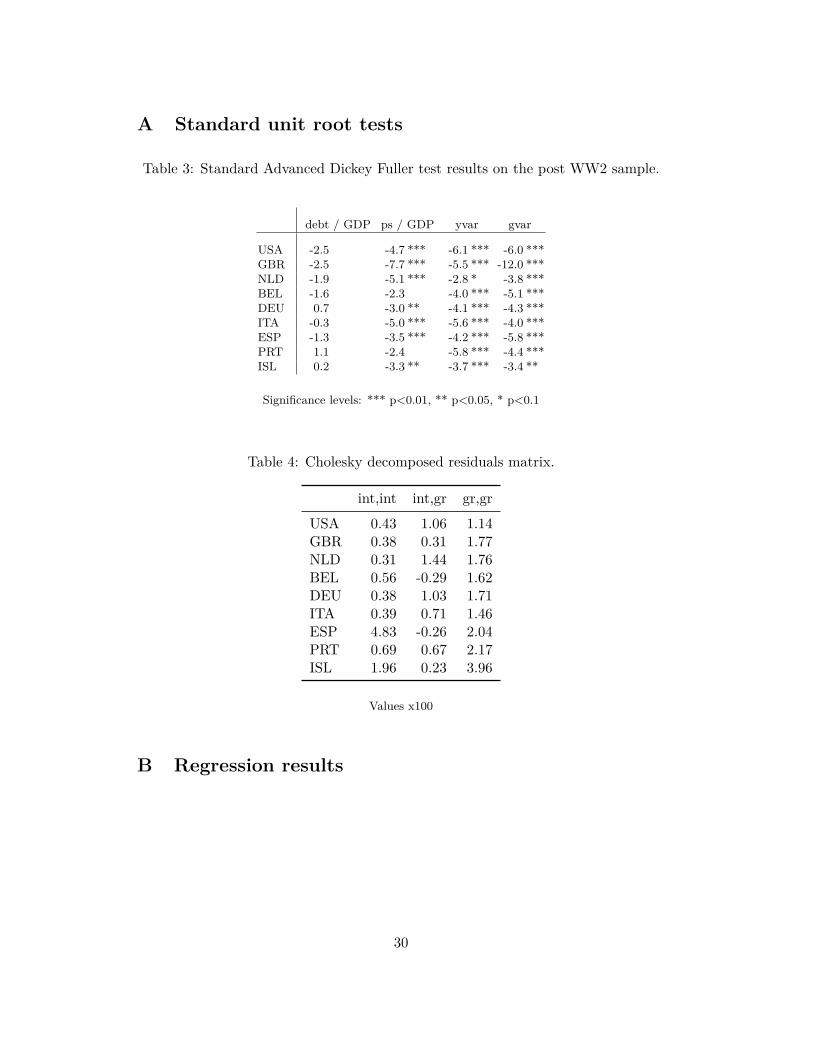
A Standard unit root tests

Table 3: Standard Advanced Dickey Fuller test results on the post WW2 sample.

debt / GDP ps / GDP yvar gvar

USA -2.5 -4.7 *** -6.1 *** -6.0 ***GBR -2.5 -7.7 *** -5.5 *** -12.0 ***NLD -1.9 -5.1 *** -2.8 * -3.8 ***BEL -1.6 -2.3 -4.0 *** -5.1 ***DEU 0.7 -3.0 ** -4.1 *** -4.3 ***ITA -0.3 -5.0 *** -5.6 *** -4.0 ***ESP -1.3 -3.5 *** -4.2 *** -5.8 ***PRT 1.1 -2.4 -5.8 *** -4.4 ***ISL 0.2 -3.3 ** -3.7 *** -3.4 **

Significance levels: *** p<0.01, ** p<0.05, * p<0.1

Table 4: Cholesky decomposed residuals matrix.

int,int int,gr gr,gr

USA 0.43 1.06 1.14GBR 0.38 0.31 1.77NLD 0.31 1.44 1.76BEL 0.56 -0.29 1.62DEU 0.38 1.03 1.71ITA 0.39 0.71 1.46ESP 4.83 -0.26 2.04PRT 0.69 0.67 2.17ISL 1.96 0.23 3.96

Values x100

B Regression results

30

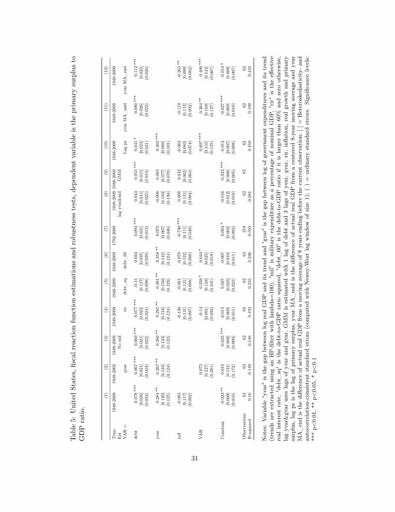
Tabl

e5:

Uni

ted

Stat

es,fi

scal

reac

tion

func

tion

estim

atio

nsan

dro

bust

ness

test

s,de

pend

ent

varia

ble

isth

epr

imar

ysu

rplu

sto

GD

Pra

tio.

(1)

(2)

(3)

(4)

(5)

(6)

(7)

(8)

(9)

(10)

(11)

(12)

Tim

e19

48-2

009

1948

-200

919

48-2

009

1948

-200

919

48-2

009

1948

-200

917

92-2

009

1948

-200

919

48-2

009

1948

-200

919

48-2

009

1948

-200

9E

stN

om

illa

gyv

ar&

mil

GM

MVA

R=

gvar

rirde

bt_

sqde

bt_

60La

gps

yvar

MA

_m

idyv

arM

A_

end

debt

0.07

8**

*0.

067

***

0.06

9**

*0.

077

***

-0.1

50.

034

0.09

4**

*0.

043

0.05

5**

*0.

041

*0.

080

***

0.11

2**

*[0

.026

][0

.021

][0

.021

][0

.023

][0

.127

][0

.035

][0

.021

][0

.041

][0

.015

][0

.023

][0

.026

][0

.025

](0

.024

)(0

.024

)(0

.022

)(0

.024

)(0

.099

)(0

.029

)(0

.013

)(0

.025

)(0

.014

)(0

.021

)(0

.023

)(0

.020

)

yvar

0.28

4**

0.26

7**

0.26

6**

0.28

5**

0.39

1**

0.35

8**

0.07

5-0

.008

0.08

50.

303

***

[0.1

20]

[0.1

23]

[0.1

23]

[0.1

24]

[0.1

50]

[0.1

42]

[0.0

67]

[0.1

93]

[0.0

77]

[0.0

89]

(0.1

25)

(0.1

24)

(0.1

23)

(0.1

24)

(0.1

29)

(0.1

24)

(0.0

46)

(0.1

30)

(0.0

70)

(0.1

01)

mil

-0.0

83-0

.136

-0.0

81-0

.078

-0.7

40**

*0.

008

0.04

2-0

.063

-0.1

19-0

.263

**[0

.117

][0

.131

][0

.121

][0

.122

][0

.111

][0

.131

][0

.062

][0

.083

][0

.112

][0

.099

](0

.092

)(0

.097

)(0

.088

)(0

.088

)(0

.049

)(0

.094

)(0

.064

)(0

.074

)(0

.092

)(0

.082

)

VAR

0.07

5-0

.14

0.23

8*

0.04

4*

0.69

7**

*0.

364

**0.

400

***

[0.2

27]

[0.0

91]

[0.1

28]

[0.0

25]

[0.1

55]

[0.1

69]

[0.1

24]

(0.2

91)

(0.0

93)

(0.1

01)

(0.0

18)

(0.1

25)

(0.1

27)

(0.0

67)

Con

stan

t-0

.023

**0.

019

-0.0

25**

*-0

.015

0.02

7-0

.007

0.00

4*

-0.0

16-0

.023

***

-0.0

12-0

.027

***

-0.0

14*

[0.0

09]

[0.1

31]

[0.0

08]

[0.0

09]

[0.0

25]

[0.0

10]

[0.0

02]

[0.0

12]

[0.0

06]

[0.0

07]

[0.0

09]

[0.0

08]

(0.0

10)

(0.1

72)

(0.0

09)

(0.0

11)

(0.0

23)

(0.0

11)

(0.0

03)

(0.0

10)

(0.0

05)

(0.0

08)

(0.0

10)

(0.0

07)

Obs

erva

tions

6262

6262

6262

218

6262

6262

62R

-squ

ared

0.16

0.14

90.

148

0.19

20.

235

0.23

60.

593

0.08

10.

458

0.19

90.

433

Not

es:

Varia

ble

"yva

r"is

the

gap

betw

een

log

real

GD

Pan

dits

tren

dan

d"g

var"

isth

ega

pbe

twee

nlo

gof

gove

rnm

ent

expe

nditu

res

and

itstr

end

(tre

nds

are

extr

acte

dus

ing

anH

P-fi

lter

with

lam

bda=

100)

,"m

il"is

mili

tary

expe

nditu

reas

ape

rcen

tage

ofno

min

alG

DP,

"rir"

isth

eeff

ectiv

ere

alin

tere

stra

te,

"deb

t_sq

"is

the

debt

-to-

GD

Pra

tiosq

uare

d,"d

ebt_

60"

isth

ede

bt-t

o-G

DP

ratio

ifit

isla

rger

than

60%

and

zero

othe

rwis

e,la

gyv

ar&

gvar

uses

lags

ofyv

aran

dgv

ar,

GM

Mis

estim

ated

with

1la

gof

debt

and

3la

gsof

yvar

,gv

ar,

rir,

infla

tion,

real

grow

than

dpr

imar

ysu

rplu

s,la

gps

isth

ela

gof

prim

ary

surp

lus,

yvar

MA

_m

idis

the

diffe

renc

eof

actu

alre

alG

DP

from

ace

nter

ed8-

year

mov

ing

aver

age

and

yvar

MA

_en

dis

the

diffe

renc

eof

actu

alre

alG

DP

from

am

ovin

gav

erag

eof

8ye

ars

endi

ngbe

fore

the

curr

ent

obse

rvat

ion;

[]=

Het

eros

keda

stic

ity-a

ndau

toco

rrel

atio

n-co

nsis

tent

stan

dard

erro

rs(c

ompu

ted

with

New

ey-W

est

lag

win

dow

ofsi

ze1)

;(

)=

ordi

nary

stan

dard

erro

rs.

Sign

ifica

nce

leve

ls:

***

p<0.

01,*

*p<

0.05

,*p<

0.1

31

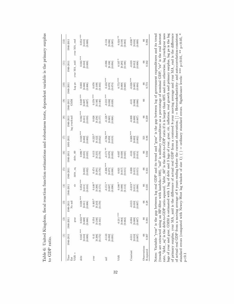
Tabl

e6:

Uni

ted

Kin

gdom

,fisc

alre

actio

nfu

nctio

nes

timat

ions

and

robu

stne

sste

sts,

depe

nden

tvar

iabl

eis

the

prim

ary

surp

lus

toG

DP

ratio

. (1)

(2)

(3)

(4)

(5)

(6)

(7)

(8)

(9)

(10)

(11)

(12)

Tim

e19

46-2

011

1946

-201

119

46-2

011

1946

-201

119

46-2

011

1946

-201

116

91-2

011

1946

-201

119

46-2

011

1946

-201

119

46-2

011

1946

-201

1E

stN

om

illa

gyv

ar&

mil

GM

MVA

R=

gvar

rirde

bt_

sqde

bt_

60La

gps

yvar

MA

_m

idyv

arM

A_

end

debt

0.04

5**

*0.

023

**0.

038

***

0.05

2**

*0.

096

*0.

049

***

0.04

2**

*0.

049

***

0.00

30.

043

***

0.05

4**

*[0

.010

][0

.009

][0

.011

][0

.011

][0

.035

][0

.055

][0

.002

][0

.011

][0

.007

][0

.008

][0

.010

][0

.013

](0

.009

)(0

.008

)(0

.008

)(0

.010

)(0

.032

)(0

.035

)(0

.002

)(0

.010

)(0

.007

)(0

.006

)(0

.009

)(0

.009

)

yvar

0.41

0.35

40.

463

*0.

446

*0.

474

0.41

3-0

.223

*0.

026

0.37

6**

*0.

076

[0.2

66]

[0.2

46]

[0.2

43]

[0.2

66]

[0.2

91]

[0.2

55]

[0.1

22]

[0.2

56]

[0.1

46]

[0.1

09]

(0.1

72)

(0.1

61)

(0.1

70)

(0.1

71)

(0.1

76)

(0.1

70)

(0.0

52)

(0.1

77)

(0.1

40)

(0.1

03)

mil

-0.1

43-0

.151

*-0

.200

***

-0.1

71**

-0.7

06**

*-0

.128

*-0

.215

***

0.43

3**

*-0

.096

-0.1

34[0

.092

][0

.087

][0

.075

][0

.078

][0

.059

][0

.065

][0

.036

][0

.078

][0

.106

][0

.096

](0

.091

)(0

.090

)(0

.098

)(0

.092

)(0

.019

)(0

.068

)(0

.039

)(0

.074

)(0

.094

)(0

.085

)

VAR

-0.2

11**

*0.

180

*0.

021

-0.0

370.

772

***

0.53

7*

0.32

4**

[0.0

64]

[0.0

99]

[0.0

17]

[0.0

39]

[0.0

68]

[0.2

85]

[0.1

59]

(0.0

63)

(0.1

13)

(0.0

15)

(0.0

25)

(0.0

69)

(0.1

88)

(0.0

83)

Con

stan

t-0

.011

-0.0

04-0

.013

-0.0

19*

0.00

9-0

.03

0.00

9**

*-0

.009

-0.0

1-0

.020

***

-0.0

19-0

.030

*[0

.010

][0

.009

][0

.010

][0

.011

][0

.015

][0

.025

][0

.003

][0

.009

][0

.006

][0

.005

][0

.012

][0

.016

](0

.007

)(0

.007

)(0

.007

)(0

.008

)(0

.015

)(0

.014

)(0

.002

)(0

.007

)(0

.006

)(0

.004

)(0

.008

)(0

.009

)

Obs

erva

tions

6666

6666

6666

321

6666

6666

66R

-squ

ared

0.30

70.

391

0.28

0.33

50.

331

0.33

20.

860.

239

0.77

30.

332

0.39

2

Not

es:

Varia

ble

"yva

r"is

the

gap

betw

een

log

real

GD

Pan

dits

tren

dan

d"g

var"

isth

ega

pbe

twee

nlo

gof

gove

rnm

ent

expe

nditu

res

and

itstr

end

(tre

nds

are

extr

acte

dus

ing

anH

P-fi

lter

with

lam

bda=

100)

,"m

il"is

mili

tary

expe

nditu

reas

ape

rcen

tage

ofno

min

alG

DP,

"rir"

isth

ere

alin

tere

stra

te,"

debt

_sq

"is

the

debt

-to-

GD

Pra

tiosq

uare

d,"d

ebt_

60"

isth

ede

bt-t

o-G

DP

ratio

ifit

isla

rger

than

60%

and

zero

othe

rwis

e,la

gyv

ar&

gvar

uses

lags

ofyv

aran

dgv

ar,G

MM

ises

timat

edw

ith1

lag

ofde

btan

d3

lags

ofyv

ar,g

var,

rir,i

nflat

ion,

real

grow

than

dpr

imar

ysu

rplu

s,la

gps

isth

ela

gof

prim

ary

surp

lus,

yvar

MA

_m

idis

the

diffe

renc

eof

actu

alre

alG

DP

from

ace

nter

ed8-

year

mov

ing

aver

age

and

yvar

MA

_en

dis

the

diffe

renc

eof

actu

alre

alG

DP

from

am

ovin

gav

erag

eof

8ye

ars

endi

ngbe

fore

the

curr

ent

obse

rvat

ion;

[]=

Het

eros

keda

stic

ity-a

ndau

toco

rrel

atio

n-co

nsis

tent

stan

dard

erro

rs(c

ompu

ted

with

New

ey-W

est

lag

win

dow

ofsi

ze1)

;(

)=

ordi

nary

stan

dard

erro

rs.

Sign

ifica

nce

leve

ls:

***

p<0.

01,*

*p<

0.05

,*p<

0.1

32

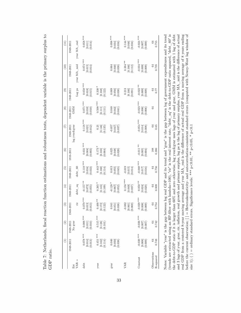
Tabl

e7:

Net

herla

nds,

fisca

lrea

ctio

nfu

nctio

nes

timat

ions

and

robu

stne

sste

sts,

depe

nden

tva

riabl

eis

the

prim

ary

surp

lus

toG

DP

ratio

.

(1)

(2)

(3)

(4)

(5)

(6)

(7)

(8)

(9)

(10)

(11)

1948

-201

119

48-2

011

1948

-201

119

48-2

011

1948

-201

118

16-2

011

1948

-201

119

48-2

011

1948

-201

119

48-2

011

1948

-201

1E

stN

ogv

arla

gyv

ar&

gvar

GM

MVA

R=

rirde

bt_

sqde

bt_

60La

gps

yvar

MA

_m

idyv

arM

A_

end

debt

0.07

8**

*0.

088

***

0.07

9**

*-0

.157

**0.

118

***

0.03

1**

*0.

118

***

0.07

1**

*0.

058

***

0.07

4**

*0.

058

***

[0.0

14]

[0.0

11]

[0.0

13]

[0.0

72]

[0.0

34]

[0.0

04]

[0.0

21]

[0.0

10]

[0.0

18]

[0.0

15]

[0.0

11]

(0.0

13)

(0.0

10)

(0.0

13)

(0.0

55)

(0.0

33)

(0.0

03)

(0.0

12)

(0.0

10)

(0.0

15)

(0.0

14)

(0.0

14)

yvar

0.45

1**

*0.

515

***

0.40

0**

0.26

5*

0.44

3**

*0.

173

*0.

210.

508

***

0.33

0*

[0.1

62]

[0.1

26]

[0.1

72]

[0.1

45]

[0.1

60]

[0.1

03]

[0.1

46]

[0.1

11]

[0.1

68]

(0.1

14)

(0.1

01)

(0.1

22)

(0.1

09)

(0.1

14)

(0.0

64)

(0.1

35)

(0.1

11)

(0.1

22)

gvar

0.04

60.

041

-0.1

28*

0.01

30.

025

-0.0

570.

048

0.06

90.

064

0.09

8**

*[0

.050

][0

.051

][0

.067

][0

.055

][0

.048

][0

.047

][0

.042

][0

.056

][0

.040

][0

.034

](0

.038

)(0

.038

)(0

.052

)(0

.045

)(0

.020

)(0

.037

)(0

.041

)(0

.038

)(0

.038

)(0

.034

)

VAR

-0.0

820.

158

***

-0.0

190.

213

0.38

4**

0.14

4**

*[0

.061

][0

.049

][0

.015

][0

.166

][0

.166

][0

.046

](0

.069

)(0

.037

)(0

.014

)(0

.091

)(0

.112

)(0

.034

)

Con

stan

t-0

.030

***

-0.0

36**

*-0

.029

***

0.05

0**

-0.0

48**

*-0

.011

**-0

.054

***

-0.0

23**

*-0

.022

**-0

.034

***

-0.0

24**

*[0

.008

][0

.007

][0

.008

][0

.024

][0

.017

][0

.005

][0

.014

][0

.006

][0

.009

][0

.009

][0

.007

](0

.009

)(0

.007

)(0

.009

)(0

.020

)(0

.016

)(0

.004

)(0

.008

)(0

.006

)(0

.009

)(0

.009

)(0

.009

)

Obs

erva

tions

6464

6464

6418

864

6464

6464

R-s

quar

ed0.

748

0.74

20.

754

0.80

90.

756

0.38

60.

650.

770.

735

0.75

5

Not

es:

Varia

ble

"yva

r"is

the

gap

betw

een

log

real

GD

Pan

dits

tren

dan

d"g

var"

isth

ega

pbe

twee

nlo

gof

gove

rnm

ent

expe

nditu

res

and

itstr

end

(tre

nds

are

extr

acte

dus

ing

anH

P-fi

lter

with

lam

bda=

100)

,"rir

"is

the

real

inte

rest

rate

,"de

bt_

sq"

isth

ede

bt-t

o-G

DP

ratio

squa

red,

"deb

t_60

"is

the

debt

-to-

GD

Pra

tioif

itis

larg

erth

an60

%an

dze

root

herw

ise,

lag

yvar

&gv

arus

esla

gsof

yvar

and

gvar

,GM

Mis

estim

ated

with

1la

gof

debt

and

3la

gsof

yvar

,gva

r,rir

,infl

atio

n,re

algr

owth

and

prim

ary

surp

lus,

lag

psis

the

lag

ofpr

imar

ysu

rplu

s,yv

arM

A_

mid

isth

edi

ffere

nce

ofac

tual

real

GD

Pfr

oma

cent

ered

8-ye

arm

ovin

gav

erag

ean

dyv

arM

A_

end

isth

edi

ffere

nce

ofac

tual

real

GD

Pfr

oma

mov

ing

aver

age

of8

year

sen

ding

befo

reth

ecu

rren

tob

serv

atio

n;[]

=H

eter

oske

dast

icity

-an

dau

toco

rrel

atio

n-co

nsis

tent

stan

dard

erro

rs(c

ompu

ted

with

New

ey-W

est

lag

win

dow

ofsi

ze1)

;()

=or

dina

ryst

anda

rder

rors

.Si

gnifi

canc

ele

vels

:**

*p<

0.01

,**

p<0.

05,*

p<0.

1

33

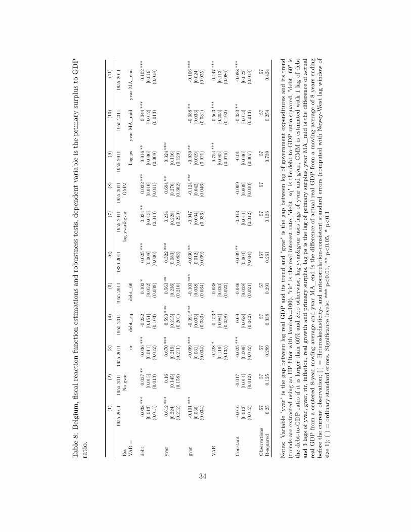
Tabl

e8:

Bel

gium

,fisc

alre

actio

nfu

nctio

nes

timat

ions

and

robu

stne

sste

sts,

depe

nden

tvar

iabl

eis

the

prim

ary

surp

lust

oG

DP

ratio

.

(1)

(2)

(3)

(4)

(5)

(6)

(7)

(8)

(9)

(10)

(11)

1955

-201

119

55-2

011

1955

-201

119

55-2

011

1955

-201

118

30-2

011

1955

-201

119

55-2

011

1955

-201

119

55-2

011

1955

-201

1E

stN

ogv

arla

gyv

ar&

gvar

GM

MVA

R=

rirde

bt_

sqde

bt_

60La

gps

yvar

MA

_m

idyv

arM

A_

end

debt

0.03

8**

*0.

037

**0.

036

***

-0.2

320.

103

*0.

025

***

0.03

4**

0.03

2**

*0.

016

**0.

044

***

0.10

2**

*[0

.013

][0

.015

][0

.011

][0

.151

][0

.052

][0

.008

][0

.013

][0

.010

][0

.006

][0

.012

][0

.019

](0

.013

)(0

.013

)(0

.012

)(0

.103

)(0

.039

)(0

.006

)(0

.013

)(0

.011

)(0

.008

)(0

.013

)(0

.018

)

yvar

0.61

2**

*0.

160.

670

***

0.59

0**

*0.

563

**0.

322

***

0.23

40.

694

**0.

324

***

[0.2

24]

[0.1

45]

[0.2

19]

[0.2

15]

[0.2

36]

[0.0

83]

[0.2

28]

[0.2

76]

[0.1

16]

(0.2

12)

(0.1

58)

(0.2

11)

(0.2

01)

(0.2

10)

(0.0

83)

(0.2

20)

(0.3

02)

(0.1

29)

gvar

-0.1

01**

*-0

.099

***

-0.0

91**

*-0

.103

***

-0.0

30**

-0.0

47-0

.124

***

-0.0

39**

-0.0

88**

-0.1

06**

*[0

.036

][0

.031

][0

.033

][0

.038

][0

.012

][0

.034

][0

.042

][0

.019

][0

.033

][0

.024

](0

.034

)(0

.034

)(0

.033

)(0

.034

)(0

.009

)(0

.036

)(0

.046

)(0

.021

)(0

.031

)(0

.025

)

VAR

0.22

8*

0.15

3*

-0.0

380.

754

***

0.56

3**

*0.

447

***

[0.1

19]

[0.0

84]

[0.0

30]

[0.0

85]

[0.2

05]

[0.1

13]

(0.1

35)

(0.0

58)

(0.0

22)

(0.0

76)

(0.1

92)

(0.0

86)

Con

stan

t-0

.016

-0.0

17-0

.025

***

0.09

-0.0

46-0

.009

**-0

.013

-0.0

09-0

.01

-0.0

30**

-0.0

88**

*[0

.012

][0

.014

][0

.009

][0

.058

][0

.028

][0

.004

][0

.011

][0

.009

][0

.006

][0

.013

][0

.022

](0

.012

)(0

.012

)(0

.012

)(0

.042

)(0

.021

)(0

.004

)(0

.012

)(0

.010

)(0

.007

)(0

.013

)(0

.018

)

Obs

erva

tions

5757

5757

5715

757

5757

5757

R-s

quar

ed0.

250.

125

0.28

90.

338

0.29

10.

261

0.13

60.

739

0.25

40.

424

Not

es:

Varia

ble

"yva

r"is

the

gap

betw

een

log

real

GD

Pan

dits

tren

dan

d"g

var"

isth

ega

pbe

twee

nlo

gof

gove

rnm

ent

expe

nditu

res

and

itstr

end

(tre

nds

are

extr

acte

dus

ing

anH

P-fi

lter

with

lam

bda=

100)

,"rir

"is

the

real

inte

rest

rate

,"de

bt_

sq"

isth

ede

bt-t

o-G

DP

ratio

squa

red,

"deb

t_60

"is

the

debt

-to-

GD

Pra

tioif

itis

larg

erth

an60

%an

dze

root

herw

ise,

lag

yvar

&gv

arus

esla

gsof

yvar

and

gvar

,GM

Mis

estim

ated

with

1la

gof

debt

and

3la

gsof

yvar

,gva

r,rir

,infl

atio

n,re

algr

owth

and

prim

ary

surp

lus,

lag

psis

the

lag

ofpr

imar

ysu

rplu

s,yv

arM

A_

mid

isth

edi

ffere

nce

ofac

tual

real

GD

Pfr

oma

cent

ered

8-ye

arm

ovin

gav

erag

ean

dyv

arM

A_

end

isth

edi

ffere

nce

ofac

tual

real

GD

Pfr

oma

mov

ing

aver

age

of8

year

sen

ding

befo

reth

ecu

rren

tob

serv

atio

n;[]

=H

eter

oske

dast

icity

-an

dau

toco

rrel

atio

n-co

nsis

tent

stan

dard

erro

rs(c

ompu

ted

with

New

ey-W

est

lag

win

dow

ofsi

ze1)

;()

=or

dina

ryst

anda

rder

rors

.Si

gnifi

canc

ele

vels

:**

*p<

0.01

,**

p<0.

05,*

p<0.

1

34

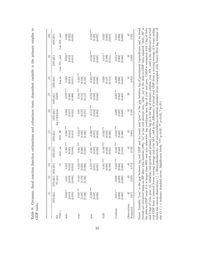
Tabl

e9:

Ger

man

y,fis

cal

reac

tion

func

tion

estim

atio

nsan

dro

bust

ness

test

s,de

pend

ent

varia

ble

isth

epr

imar

ysu

rplu

sto

GD

Pra

tio.

(1)

(2)

(3)

(4)

(5)

(6)

(7)

(8)

(9)

(10)

1970

-201

119

70-2

011

1970

-201

119

70-2

011

1970

-201

119

70-2

011

1970

-201

119

70-2

011

1970

-201

119

70-2

011

Est

No

gvar

lag

yvar

&gv

arG

MM

VAR

=rir

debt

_sq

debt

_60

Lag

psyv

arM

A_

mid

yvar

MA

_en

d

debt

0.02

6*

0.02

10.

012

0.20

5**

*0.

050

***

0.02

20.

019

***

0.02

30.

028

*0.

026

[0.0

13]

[0.0

19]

[0.0

10]

[0.0

45]

[0.0

14]

[0.0

17]

[0.0

06]

[0.0

14]

[0.0

14]

[0.0

22]

(0.0

10)

(0.0

16)

(0.0

10)

(0.0

48)

(0.0

14)

(0.0

16)

(0.0

06)

(0.0

11)

(0.0

11)

(0.0

18)

yvar

0.22

7**

0.14

30.

345

***

0.26

1**

*0.

233

**-0

.07

0.34

1**

*0.

237

**[0

.107

][0

.178

][0

.095

][0

.086

][0

.105

][0

.127

][0

.112

][0

.108

](0

.106

)(0

.162

)(0

.098

)(0

.091

)(0

.100

)(0

.157

)(0

.113

)(0

.108

)

gvar

-0.2

60**

*-0

.275

***

-0.2

61**

*-0

.269

***

-0.1

19**

*-0

.278

***

-0.2

65**

*-0

.248

***

-0.2

52**

*[0

.047

][0

.051

][0

.053

][0

.051

][0

.042

][0

.030

][0

.058

][0

.047

][0

.051

](0

.035

)(0

.031

)(0

.030

)(0

.033

)(0

.052

)(0

.030

)(0

.040

)(0

.035

)(0

.037

)

VAR

0.36

1**

*-0

.196

***

-0.0

22**

0.02

80.

215

*0.

025

[0.0

88]

[0.0

46]

[0.0

10]

[0.1

27]

[0.1

08]

[0.0

82]

(0.1

00)

(0.0

51)

(0.0

09)

(0.1

14)

(0.1

11)

(0.0

73)

Con

stan

t-0

.011

*-0

.009

-0.0

18**

*-0

.045

***

-0.0

18**

*-0

.009

-0.0

07**

-0.0

09-0

.014

**-0

.011

[0.0

06]

[0.0

09]

[0.0

04]

[0.0

09]

[0.0

05]

[0.0

07]

[0.0

03]

[0.0

06]

[0.0

06]

[0.0

08]

(0.0

05)

(0.0

08)

(0.0

05)

(0.0

10)

(0.0

06)

(0.0

08)

(0.0

03)

(0.0

05)

(0.0

06)

(0.0

08)

Obs

erva

tions

4242

4242

4241

3941

4242

R-s

quar

ed0.

611

0.05

30.

713

0.72

20.

664

0.16

80.

623

0.60

30.

565

Not

es:

Varia

ble

"yva

r"is

the

gap

betw

een

log

real

GD

Pan

dits

tren

dan

d"g

var"

isth

ega

pbe

twee

nlo

gof

gove

rnm

ent

expe

nditu

res

and

itstr

end

(tre

nds

are

extr

acte

dus

ing

anH

P-fi

lter

with

lam

bda=

100)

,"rir

"is

the

real

inte

rest

rate

,"de

bt_

sq"

isth

ede

bt-t

o-G

DP

ratio

squa

red,

"deb

t_60

"is

the

debt

-to-

GD

Pra

tioif

itis

larg

erth

an60

%an

dze

root

herw

ise,

lag

yvar

&gv

arus

esla

gsof

yvar

and

gvar

,GM

Mis

estim

ated

with

1la

gof

debt

and

3la

gsof

yvar

,gva

r,rir

,infl

atio

n,re

algr

owth

and

prim

ary

surp

lus,

lag

psis

the

lag

ofpr

imar

ysu

rplu

s,yv

arM

A_

mid

isth

edi

ffere

nce

ofac

tual

real

GD

Pfr

oma

cent

ered

8-ye

arm

ovin

gav

erag

ean

dyv

arM

A_

end

isth

edi

ffere

nce

ofac

tual

real

GD

Pfr

oma

mov

ing

aver

age

of8

year

sen

ding

befo

reth

ecu

rren

tob

serv

atio

n;[]

=H

eter

oske

dast

icity

-an

dau

toco

rrel

atio

n-co

nsis

tent

stan

dard

erro

rs(c

ompu

ted

with

New

ey-W

est

lag

win

dow

ofsi

ze1)

;()

=or

dina

ryst

anda

rder

rors

.Si

gnifi

canc

ele

vels

:**

*p<

0.01

,**

p<0.

05,*

p<0.

1

35

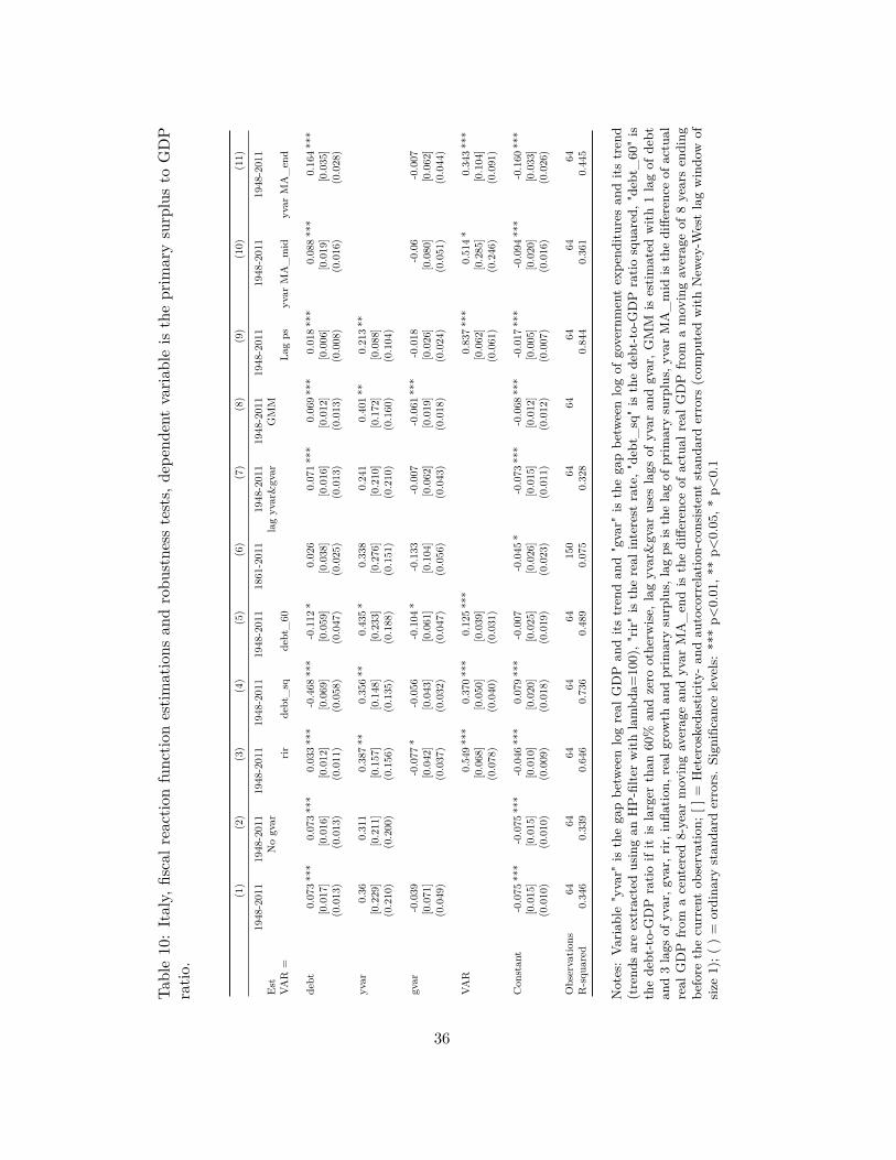
Tabl

e10

:It

aly,

fisca

lrea

ctio

nfu

nctio

nes

timat

ions

and

robu

stne

sste

sts,

depe

nden

tva

riabl

eis

the

prim

ary

surp

lus

toG

DP

ratio

.

(1)

(2)

(3)

(4)

(5)

(6)

(7)

(8)

(9)

(10)

(11)

1948

-201

119

48-2

011

1948

-201

119

48-2

011

1948

-201

118

61-2

011

1948

-201

119

48-2

011

1948

-201

119

48-2

011

1948

-201

1E

stN

ogv

arla

gyv

ar&

gvar

GM

MVA

R=

rirde

bt_

sqde

bt_

60La

gps

yvar

MA

_m

idyv

arM

A_

end

debt

0.07

3**

*0.

073

***

0.03

3**

*-0

.468

***

-0.1

12*

0.02

60.

071

***

0.06

9**

*0.

018

***

0.08

8**

*0.

164

***

[0.0

17]

[0.0

16]

[0.0

12]

[0.0

69]

[0.0

59]

[0.0

38]

[0.0

16]

[0.0

12]

[0.0

06]

[0.0

19]

[0.0

35]

(0.0

13)

(0.0

13)

(0.0

11)

(0.0

58)

(0.0

47)

(0.0

25)

(0.0

13)

(0.0

13)

(0.0

08)

(0.0

16)

(0.0

28)

yvar

0.36

0.31

10.

387

**0.

356

**0.

435

*0.

338

0.24

10.

401

**0.

213

**[0

.229

][0

.211

][0

.157

][0

.148

][0

.233

][0

.276

][0

.210

][0

.172

][0

.088

](0

.210

)(0

.200

)(0

.156

)(0

.135

)(0

.188

)(0

.151

)(0

.210

)(0

.160

)(0

.104

)

gvar

-0.0

39-0

.077

*-0

.056

-0.1

04*

-0.1

33-0

.007

-0.0

61**

*-0

.018

-0.0

6-0

.007

[0.0

71]

[0.0

42]

[0.0

43]

[0.0

61]

[0.1

04]

[0.0

62]

[0.0

19]

[0.0

26]

[0.0

80]

[0.0

62]

(0.0

49)

(0.0

37)

(0.0

32)

(0.0

47)

(0.0

56)

(0.0

43)

(0.0

18)

(0.0

24)

(0.0

51)

(0.0

44)

VAR

0.54

9**

*0.

370

***

0.12

5**

*0.

837

***

0.51

4*

0.34

3**

*[0

.068

][0

.050

][0

.039

][0

.062

][0

.285

][0

.104

](0

.078

)(0

.040

)(0

.031

)(0

.061

)(0

.246

)(0

.091

)

Con

stan

t-0

.075

***

-0.0

75**

*-0

.046

***

0.07

9**

*-0

.007

-0.0

45*

-0.0

73**

*-0

.068

***

-0.0

17**

*-0

.094

***

-0.1

60**

*[0

.015

][0

.015

][0

.010

][0

.020

][0

.025

][0

.026

][0

.015

][0

.012

][0

.005

][0

.020

][0

.033

](0

.010

)(0

.010

)(0

.009

)(0

.018

)(0

.019

)(0

.023

)(0

.011

)(0

.012

)(0

.007

)(0

.016

)(0

.026

)

Obs

erva

tions

6464

6464

6415

064

6464

6464

R-s

quar

ed0.

346

0.33

90.

646

0.73

60.

489

0.07

50.

328

0.84

40.

361

0.44

5

Not

es:

Varia

ble

"yva

r"is

the

gap

betw

een

log

real

GD

Pan

dits

tren

dan

d"g

var"

isth

ega

pbe

twee

nlo

gof

gove

rnm

ent

expe

nditu

res

and

itstr

end

(tre

nds

are

extr

acte

dus

ing

anH

P-fi

lter

with

lam

bda=

100)

,"rir

"is

the

real

inte

rest

rate

,"de

bt_

sq"

isth

ede

bt-t

o-G

DP

ratio

squa

red,

"deb

t_60

"is

the

debt

-to-

GD

Pra

tioif

itis

larg

erth

an60

%an

dze

root

herw

ise,

lag

yvar

&gv

arus

esla

gsof

yvar

and

gvar

,GM

Mis

estim

ated

with

1la

gof

debt

and

3la

gsof

yvar

,gva

r,rir

,infl

atio

n,re

algr

owth

and

prim

ary

surp

lus,

lag

psis

the

lag

ofpr

imar

ysu

rplu

s,yv

arM

A_

mid

isth

edi

ffere

nce

ofac

tual

real

GD

Pfr

oma

cent

ered

8-ye

arm

ovin

gav

erag

ean

dyv

arM

A_

end

isth

edi

ffere

nce

ofac

tual

real

GD

Pfr

oma

mov

ing

aver

age

of8

year

sen

ding

befo

reth

ecu

rren

tob

serv

atio

n;[]

=H

eter

oske

dast

icity

-an

dau

toco

rrel

atio

n-co

nsis

tent

stan

dard

erro

rs(c

ompu

ted

with

New

ey-W

est

lag

win

dow

ofsi

ze1)

;()

=or

dina

ryst

anda

rder

rors

.Si

gnifi

canc

ele

vels

:**

*p<

0.01

,**

p<0.

05,*

p<0.

1

36

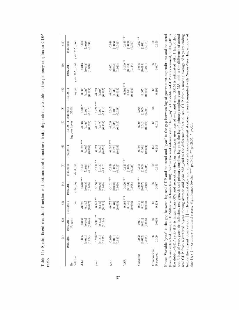
Tabl

e11

:Sp

ain,

fisca

lrea

ctio

nfu

nctio

nes

timat

ions

and

robu

stne

sste

sts,

depe

nden

tva

riabl

eis

the

prim

ary

surp

lus

toG

DP

ratio

.

(1)

(2)

(3)

(4)

(5)

(6)

(7)

(8)

(9)

(10)

(11)

1946

-201

119

46-2

011

1946

-201

119

46-2

011

1946

-201

118

50-2

011

1946

-201

119

46-2

011

1946

-201

119

46-2

011

1946

-201

1E

stN

ogv

arla

gyv

ar&

gvar

GM

MVA

R=

rirde

bt_

sqde

bt_

60La

gps

yvar

MA

_m

idyv

arM

A_

end

debt

0.00

50.

008

-0.0

260.

540

***

0.05

30.

025

***

-0.0

070.

031

*0.

003

0.01

30.

056

[0.0

41]

[0.0

40]

[0.0

40]

[0.0

58]

[0.0

35]

[0.0

05]

[0.0

46]

[0.0

17]

[0.0

21]

[0.0

44]

[0.0

39]

(0.0

24)

(0.0

24)

(0.0

22)

(0.0

66)

(0.0

23)

(0.0

05)

(0.0

25)

(0.0

15)

(0.0

19)

(0.0

26)

(0.0

31)

yvar

0.29

8**

0.32

1**

0.34

2**

0.15

0*

0.23

2**

0.07

7-0

.016

0.47

1**

*-0

.021

[0.1

41]

[0.1

35]

[0.1

47]

[0.0

79]

[0.1

05]

[0.0

63]

[0.1

78]

[0.0

97]

[0.1

08]

(0.1

27)

(0.1

24)

(0.1

11)

(0.0

89)

(0.1

10)

(0.0

51)

(0.1

34)

(0.1

14)

(0.1

07)

gvar

-0.0

39-0

.075

**-0

.101

***

-0.0

58-0

.085

***

-0.0

380.

015

-0.0

35-0

.051

-0.0

48[0

.041

][0

.037

][0

.030

][0

.035

][0

.029

][0

.038

][0

.041

][0

.033

][0

.038

][0

.033

](0

.043

)(0

.038

)(0

.030

)(0

.037

)(0

.019

)(0

.045

)(0

.038

)(0

.033

)(0

.043

)(0

.041

)

VAR

0.16

6**

*-0

.820

***

-0.1

20**

*0.

704

***

0.30

9**

0.15

5**

*[0

.048

][0

.104

][0

.025

][0

.143

][0

.134

][0

.033

](0

.036

)(0

.098

)(0

.025

)(0

.104

)(0

.144

)(0

.050

)

Con

stan

t0.

002

0.00

10.

011

-0.0

69**

*-0

.011

-0.0

050.

005

-0.0

05-0

.008

-0.0

27**

[0.0

12]

[0.0

11]

[0.0

11]

[0.0

07]

[0.0

09]

[0.0

04]

[0.0

13]

[0.0

05]

[0.0

05]

[0.0

13]

[0.0

11]

(0.0

08)

(0.0

08)

(0.0

08)

(0.0

10)

(0.0

08)

(0.0

04)

(0.0

09)

(0.0

05)

(0.0

06)

(0.0

11)

(0.0

13)

Obs

erva

tions

6666

6666

6615

666

6666

6666

R-s

quar

ed0.

109

0.09

80.

338

0.58

70.

353

0.24

30.

013

0.49

20.

097

0.15

9

Not

es:

Varia

ble

"yva

r"is

the

gap

betw

een

log

real

GD

Pan

dits

tren

dan

d"g

var"

isth

ega

pbe

twee

nlo

gof

gove

rnm

ent

expe

nditu

res

and

itstr

end

(tre

nds

are

extr

acte

dus

ing

anH

P-fi

lter

with

lam

bda=

100)

,"rir

"is

the

real

inte

rest

rate

,"de

bt_

sq"

isth

ede

bt-t

o-G

DP

ratio

squa

red,

"deb

t_60

"is

the

debt

-to-

GD

Pra

tioif

itis

larg

erth

an60

%an

dze

root

herw

ise,

lag

yvar

&gv

arus

esla

gsof

yvar

and

gvar

,GM

Mis

estim

ated

with

1la

gof

debt

and

3la

gsof

yvar

,gva

r,rir

,infl

atio

n,re

algr

owth

and

prim

ary

surp

lus,

lag

psis

the

lag

ofpr

imar

ysu

rplu

s,yv

arM

A_

mid

isth

edi

ffere

nce

ofac

tual

real

GD

Pfr

oma

cent

ered

8-ye

arm

ovin

gav

erag

ean

dyv

arM

A_

end

isth

edi

ffere

nce

ofac

tual

real

GD

Pfr

oma

mov

ing

aver

age

of8

year

sen

ding

befo

reth

ecu

rren

tob

serv

atio

n;[]

=H

eter

oske

dast

icity

-an

dau

toco

rrel

atio

n-co

nsis

tent

stan

dard

erro

rs(c

ompu

ted

with

New

ey-W

est

lag

win

dow

ofsi

ze1)

;()

=or

dina

ryst

anda

rder

rors

.Si

gnifi

canc

ele

vels

:**

*p<

0.01

,**

p<0.

05,*

p<0.

1

37

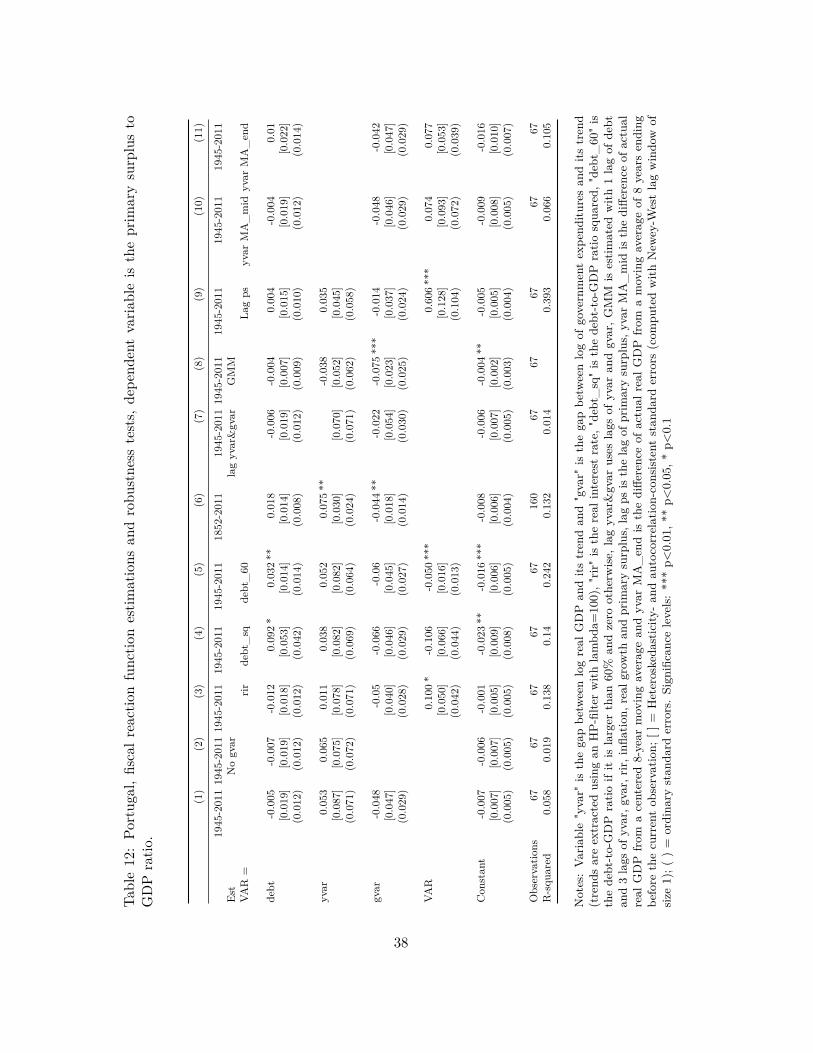
Tabl

e12

:Po

rtug

al,

fisca

lrea

ctio

nfu

nctio

nes

timat

ions

and

robu

stne

sste

sts,

depe

nden

tva

riabl

eis

the

prim

ary

surp

lus

toG

DP

ratio

.

(1)

(2)

(3)

(4)

(5)

(6)

(7)

(8)

(9)

(10)

(11)

1945

-201

119

45-2

011

1945

-201

119

45-2

011

1945

-201

118

52-2

011

1945

-201

119

45-2

011

1945

-201

119

45-2

011

1945

-201

1E

stN

ogv

arla

gyv

ar&

gvar

GM

MVA

R=

rirde

bt_

sqde

bt_

60La

gps

yvar

MA

_m

idyv

arM

A_

end

debt

-0.0

05-0

.007

-0.0

120.

092

*0.

032

**0.

018

-0.0

06-0

.004

0.00

4-0

.004

0.01

[0.0

19]

[0.0

19]

[0.0

18]

[0.0

53]

[0.0

14]

[0.0

14]

[0.0

19]

[0.0

07]

[0.0

15]

[0.0

19]

[0.0

22]

(0.0

12)

(0.0

12)

(0.0

12)

(0.0

42)

(0.0

14)

(0.0

08)

(0.0

12)

(0.0

09)

(0.0

10)

(0.0

12)

(0.0

14)

yvar

0.05

30.

065

0.01

10.

038

0.05

20.

075

**-0

.038

0.03

5[0

.087

][0

.075

][0

.078

][0

.082

][0

.082

][0

.030

][0

.070

][0

.052

][0

.045

](0

.071

)(0

.072

)(0

.071

)(0

.069

)(0

.064

)(0

.024

)(0

.071

)(0

.062

)(0

.058

)

gvar

-0.0

48-0

.05

-0.0

66-0

.06

-0.0

44**

-0.0

22-0

.075

***

-0.0

14-0

.048

-0.0

42[0

.047

][0

.040

][0

.046

][0

.045

][0

.018

][0

.054

][0

.023

][0

.037

][0

.046

][0

.047

](0

.029

)(0

.028

)(0

.029

)(0

.027

)(0

.014

)(0

.030

)(0

.025

)(0

.024

)(0

.029

)(0

.029

)

VAR

0.10

0*

-0.1

06-0

.050

***

0.60

6**

*0.

074

0.07

7[0

.050

][0

.066

][0

.016

][0

.128

][0

.093

][0

.053

](0

.042

)(0

.044

)(0

.013

)(0

.104

)(0

.072

)(0

.039

)

Con

stan

t-0

.007

-0.0

06-0

.001

-0.0

23**

-0.0

16**

*-0

.008

-0.0

06-0

.004

**-0

.005

-0.0

09-0

.016

[0.0

07]

[0.0

07]

[0.0

05]

[0.0

09]

[0.0

06]

[0.0

06]

[0.0

07]

[0.0

02]

[0.0

05]

[0.0

08]

[0.0

10]

(0.0

05)

(0.0

05)

(0.0

05)

(0.0

08)

(0.0

05)

(0.0

04)

(0.0

05)

(0.0

03)

(0.0

04)

(0.0

05)

(0.0

07)

Obs

erva

tions

6767

6767

6716

067

6767

6767

R-s

quar

ed0.

058

0.01

90.

138

0.14

0.24

20.

132

0.01

40.

393

0.06

60.

105

Not

es:

Varia

ble

"yva

r"is

the

gap

betw

een

log

real

GD

Pan

dits

tren

dan

d"g

var"

isth

ega

pbe

twee

nlo

gof

gove

rnm

ent

expe

nditu

res

and

itstr

end

(tre

nds

are

extr

acte

dus

ing

anH

P-fi

lter

with

lam

bda=

100)

,"rir

"is

the

real

inte

rest

rate

,"de

bt_

sq"

isth

ede

bt-t

o-G

DP

ratio

squa

red,

"deb

t_60

"is

the

debt

-to-

GD

Pra

tioif

itis

larg

erth

an60

%an

dze

root

herw

ise,

lag

yvar

&gv

arus

esla

gsof

yvar

and

gvar

,GM

Mis

estim

ated

with

1la

gof

debt

and

3la

gsof

yvar

,gva

r,rir

,infl

atio

n,re

algr

owth

and

prim

ary

surp

lus,

lag

psis

the

lag

ofpr

imar

ysu

rplu

s,yv

arM

A_

mid

isth

edi

ffere

nce

ofac

tual

real

GD

Pfr

oma

cent

ered

8-ye

arm

ovin

gav

erag

ean

dyv

arM

A_

end

isth

edi

ffere

nce

ofac

tual

real

GD

Pfr

oma

mov

ing

aver

age

of8

year

sen

ding

befo

reth

ecu

rren

tob

serv

atio

n;[]

=H

eter

oske

dast

icity

-an

dau

toco

rrel

atio

n-co

nsis

tent

stan

dard

erro

rs(c

ompu

ted

with

New

ey-W

est

lag

win

dow

ofsi

ze1)

;()

=or

dina

ryst

anda

rder

rors

.Si

gnifi

canc

ele

vels

:**

*p<

0.01

,**

p<0.

05,*

p<0.

1

38

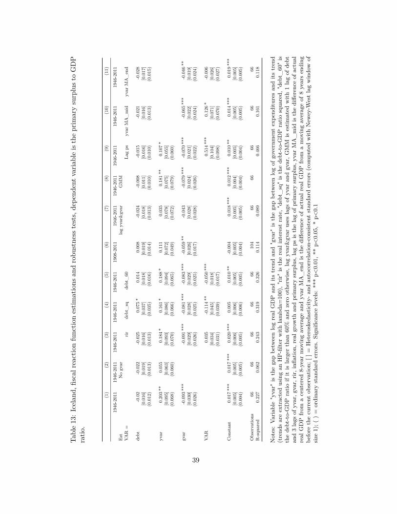
Tabl

e13

:Ic

elan

d,fis

calr

eact

ion

func

tion

estim

atio

nsan

dro

bust

ness

test

s,de

pend

entv

aria

ble

isth

epr

imar

ysu

rplu

sto

GD

Pra

tio.

(1)

(2)

(3)

(4)

(5)

(6)

(7)

(8)

(9)

(10)

(11)

1946

-201

119

46-2

011

1946

-201

119

46-2

011

1946

-201

119

08-2

011

1946

-201

119

46-2

011

1946

-201

119

46-2

011

1946

-201

1E

stN

ogv

arla

gyv

ar&

gvar

GM

MVA

R=

rirde

bt_

sqde

bt_

60La

gps

yvar

MA

_m

idyv

arM

A_

end

debt

-0.0

2-0

.022

-0.0

250.

075

*0.

014

0.00

8-0

.024

-0.0

08-0

.015

-0.0

21-0

.028

[0.0

16]

[0.0

19]

[0.0

16]

[0.0

37]

[0.0

18]

[0.0

19]

[0.0

18]

[0.0

11]

[0.0

16]

[0.0

16]

[0.0

17]

(0.0

12)

(0.0

13)

(0.0

13)

(0.0

35)

(0.0

16)

(0.0

14)

(0.0

13)

(0.0

10)

(0.0

10)

(0.0

13)

(0.0

15)

yvar

0.20

3**

0.05

50.

184

*0.

161

*0.

188

*0.

111

0.03

50.

181

**0.

107

*[0

.095

][0

.063

][0

.093

][0

.086

][0

.094

][0

.072

][0

.078

][0

.075

][0

.055

](0

.068

)(0

.060

)(0

.070

)(0

.066

)(0

.065

)(0

.049

)(0

.072

)(0

.079

)(0

.060

)

gvar

-0.0

93**

*-0

.091

***

-0.0

81**

*-0

.083

***

-0.0

59**

-0.0

43-0

.079

***

-0.0

70**

*-0

.065

***

-0.0

46**

[0.0

30]

[0.0

29]

[0.0

28]

[0.0

29]

[0.0

26]

[0.0

28]

[0.0

24]

[0.0

21]

[0.0

22]

[0.0

19]

(0.0

26)

(0.0

26)

(0.0

25)

(0.0

25)

(0.0

17)

(0.0

28)

(0.0

26)

(0.0

22)

(0.0

24)

(0.0

24)

VAR

0.03

5-0

.114

**-0

.050

***

0.51

4**

*0.

126

*-0

.006

[0.0

34]

[0.0

45]

[0.0

18]

[0.1

04]

[0.0

71]

[0.0

26]

(0.0

31)

(0.0

39)

(0.0

17)

(0.0

98)

(0.0

70)

(0.0

27)

Con

stan

t0.

017

***

0.01

7**

*0.

020

***

0.00

50.

010

**-0

.004

0.01

8**

*0.

012

***

0.01

0**

0.01

4**

*0.

019

***

[0.0

05]

[0.0

05]

[0.0

06]

[0.0

06]

[0.0

05]

[0.0

05]

[0.0

05]

[0.0

04]

[0.0

05]

[0.0

05]

[0.0

05]

(0.0

04)

(0.0

05)

(0.0

05)

(0.0

06)

(0.0

05)

(0.0

04)

(0.0

05)

(0.0

04)

(0.0

04)

(0.0

05)

(0.0

05)

Obs

erva

tions

6666

6666

6610

466

6666

6666

R-s

quar

ed0.

227

0.06

20.

243

0.31

90.

326

0.11

40.

089

0.46

60.

161

0.11

8

Not

es:

Varia

ble

"yva

r"is

the

gap

betw

een

log

real

GD

Pan

dits

tren

dan

d"g

var"

isth

ega

pbe

twee

nlo

gof

gove

rnm

ent

expe

nditu

res

and

itstr

end

(tre

nds

are

extr

acte

dus

ing

anH

P-fi

lter

with

lam

bda=

100)

,"rir

"is

the

real

inte

rest

rate

,"de

bt_

sq"

isth

ede

bt-t

o-G

DP

ratio

squa

red,

"deb

t_60

"is

the

debt

-to-

GD

Pra

tioif

itis

larg

erth

an60

%an

dze

root

herw

ise,

lag

yvar

&gv

arus

esla

gsof

yvar

and

gvar

,GM

Mis

estim

ated

with

1la

gof

debt

and

3la

gsof

yvar

,gva

r,rir

,infl

atio

n,re

algr

owth

and

prim

ary

surp

lus,

lag

psis

the

lag

ofpr

imar

ysu

rplu

s,yv

arM

A_

mid

isth

edi

ffere

nce

ofac

tual

real

GD

Pfr

oma

cent

ered

8-ye

arm

ovin

gav

erag

ean

dyv

arM

A_

end

isth

edi

ffere

nce

ofac

tual

real

GD

Pfr

oma

mov

ing

aver

age

of8

year

sen

ding

befo

reth

ecu

rren

tob

serv

atio

n;[]

=H

eter

oske

dast

icity

-an

dau

toco

rrel

atio

n-co

nsis

tent

stan

dard

erro

rs(c

ompu

ted

with

New

ey-W

est

lag

win

dow

ofsi

ze1)

;()

=or

dina

ryst

anda

rder

rors

.Si

gnifi

canc

ele

vels

:**

*p<

0.01

,**

p<0.

05,*

p<0.

1

39

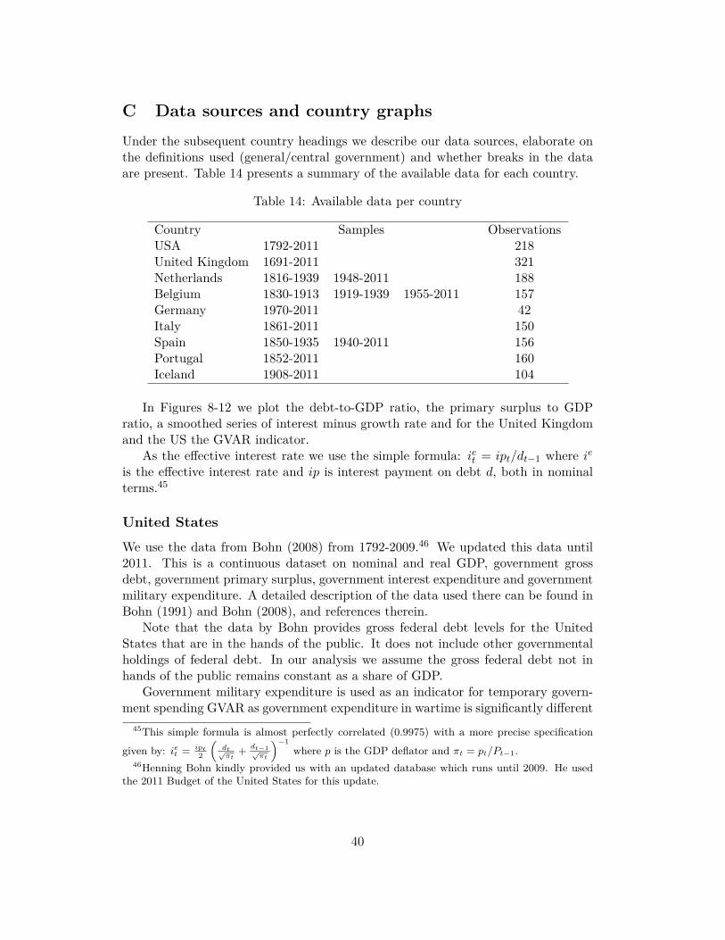
C Data sources and country graphsUnder the subsequent country headings we describe our data sources, elaborate onthe definitions used (general/central government) and whether breaks in the dataare present. Table 14 presents a summary of the available data for each country.

Table 14: Available data per country

Country Samples ObservationsUSA 1792-2011 218United Kingdom 1691-2011 321Netherlands 1816-1939 1948-2011 188Belgium 1830-1913 1919-1939 1955-2011 157Germany 1970-2011 42Italy 1861-2011 150Spain 1850-1935 1940-2011 156Portugal 1852-2011 160Iceland 1908-2011 104

In Figures 8-12 we plot the debt-to-GDP ratio, the primary surplus to GDPratio, a smoothed series of interest minus growth rate and for the United Kingdomand the US the GVAR indicator.

As the effective interest rate we use the simple formula: 𝑖𝑒𝑡 = 𝑖𝑝𝑡/𝑑𝑡−1 where 𝑖𝑒

is the effective interest rate and 𝑖𝑝 is interest payment on debt 𝑑, both in nominalterms.45

United States

We use the data from Bohn (2008) from 1792-2009.46 We updated this data until2011. This is a continuous dataset on nominal and real GDP, government grossdebt, government primary surplus, government interest expenditure and governmentmilitary expenditure. A detailed description of the data used there can be found inBohn (1991) and Bohn (2008), and references therein.

Note that the data by Bohn provides gross federal debt levels for the UnitedStates that are in the hands of the public. It does not include other governmentalholdings of federal debt. In our analysis we assume the gross federal debt not inhands of the public remains constant as a share of GDP.

Government military expenditure is used as an indicator for temporary govern-ment spending GVAR as government expenditure in wartime is significantly different

45This simple formula is almost perfectly correlated (0.9975) with a more precise specification

given by: 𝑖𝑒𝑡 = 𝑖𝑝𝑡

2

(︁𝑑𝑡√𝜋𝑡

+ 𝑑𝑡−1√𝜋𝑡

)︁−1where 𝑝 is the GDP deflator and 𝜋𝑡 = 𝑝𝑡/𝑃𝑡−1.

46Henning Bohn kindly provided us with an updated database which runs until 2009. He usedthe 2011 Budget of the United States for this update.

40

from government spending in peacetime. Using dummy variables for the war years47

instead of actual military expenditure does not change the results significantly.

United Kingdom

The sample from the United Kingdom is from 1692-2011 with a break in 1800 andin 1946. There is a shift in the reporting year in 1800, prior to 1946 we use centralgovernment data and after 1946 we use general government data. We use militaryexpenditure as a proxy for temporary government spending and there is a break inthis series in 1980 probably due to a different specification. Prior to 1946 militaryexpenditure and interest expenditure are the only two large items on the central gov-ernments budget. Non-military non-interest spending never exceeds 2% of GDP.48

Data is obtained from six sources:

∙ Data on central government expenditure (1692-1945), interest expenditure(1692-1945), military expenditure (1692-1980), revenue (1692-1946), publicdebt (1692-1979), CPI as a proxy for the GDP deflator (1691-1792), a GDPdeflator (1830-1946) and nominal GDP (1830-1946) has been obtained fromMichell (1988).

∙ From Peacock and Wiseman (1961) real and nominal GDP is obtained for theyears 1792, 1800, 1814, 1822, 1831. Constant growth rates in real and nominalGDP are assumed between these dates.

∙ Real GDP for 1700 and 1800 is obtained from Maddison (2003) world historictables. Constant growth rates in real GDP is assumed between 1700 and 1792and in the period 1691-1700.

∙ General government expenditure, interest expenditure, revenue and real andnominal GDP from 1946 onwards is obtained from the Office of National Statis-tics

∙ Public debt is obtained from the United Kingdom Ministry of Finance for1980-2011

∙ Military expenditure for 1980-2011 is obtained from the OECD.

A GDP deflator and real GDP from 1692-2011 is obtained by coupling the variouspartial GDP series with each other. Furthermore GDP has been adjusted suchthat Ireland is excluded prior to 1920 as it is after 1920. Temporary governmentexpenditure GVAR is military spending. As an alternative we use gap between thelog of government expenditure and its trend.

471812-1815 War of 1812, 1846-1849 (Mexican-American War), 1861-1865 (American Civil War),1917-1920 (World War I), 1940-1945 (World War II)

48Except for 1836 and 1837. In these years the government compensated slave owners for out-lawing slavery.

41

Netherlands

Data is obtained from Bos (2007) and contains nominal GDP, a piecewise continuousGDP deflator, gross government debt and a decomposition of government revenueand government expenditure in their main components. It runs from 1815 till 2009with gaps in the inter-war years. Bos (2007)acquires data on general governmentfinances in the period 1815-1900 from the work of van Zanden (1996) and from 1900onwards from Statistics Netherlands. In the period 1850-1900 only data on centralgovernment finances are available. Furthermore data on local government interestexpenditure is missing until 1947.

We correct for that by using two assumptions. First, we assume that the interestrate on non-central government debt equals the interest rate on central governmentdebt. In the Netherlands, the central government steps in and assumes full liabilitywhen local governments are in financial distress. Therefore local government de-fault risk is equal to central government default risk. Second we assume that localgovernment finances have run a balanced budget, as they are required by law, andwe interpolate non-central government debt between 1850 and 1900 linearly. Thisseems a reasonable first assumption as in 1850 non-central government debt is 26.0%of general government debt, in 1900 it is 20.2%. If these assumptions underestimatelocal interest expenditure, primary surplus and implied interest rates prior to 1947would be lower than their actual value. The effect on debt sustainability will beabsent, as primary surplus and the implied interest rates have opposite signs in theaccounting equation. This has been tested by using central instead of general gov-ernment finances. As none of the regression coefficients except for the constant tochanged by more than one standard deviation, we deem these assumptions reason-able.

Bos (2007) provides GDP deflators from 1815-1913, 1921-1939 and 1948-2009,Statistics Netherlands (CBS, 1959, 1994, 2001) provides a consumer price index from1900-2009. A continuous GDP deflator is constructed by using consumer price in-dices to bridge the gap between the broken piece-wise continuous GDP deflators. Weapproximate the GDP deflator from 1913-1921 and from 1939-1948 by the consumerprice index. The consumer price index is highly correlated with the GDP deflatorin the period 1900-1913, 1922-1939 and 1949-2009: correlation is 0.998 on level and0.949 on first differences.

Temporary government expenditure is defined as the residual of government ex-penditure after its HP-filtered mean has been removed. Note that Bohn (2008)uses military expenditure as an alternative measure of temporary government ex-penditure. Unlike the United States, where military spending drives governmentspending prior to 1948, the only notable Dutch event is the Belgian war of indepen-dence in 1830. Wierts and Schotten (2008) argue gas revenue should be used from1970s onwards as it had considerable impact in budgetary policy. Both alternativespecifications are used in robustness checks and do not provide significant changes.

42

Belgium

The sample from Belgium is from 1830-1913, 1920-1939 and 1955-2011 with a breakin 1970. Prior to 1970 central government data is used, after 1970 general govern-ment data. Data for Belgium has been obtained from 4 sources:

∙ A dataset on Belgium’s central government finances from the independence ofthe state in 1830 until the first world war (1913) was created by Joseph Pi-rard and published in Pirard (1999). He reports central government revenue,expenditure, gross government debt, interest expenditure nominal GDP from1830 onwards. In this book Pirard also publishes this data for the Inter bellum(1920-1939) and the years after the Second World War (1945-1995), which heobtains from other sources. finance data after 1945 as the increase in debt isalways smaller than the difference between government revenue and govern-ment expenditure and much to persistent to be due to stock-flow adjustments.This might be due to the fact that some government bond redemptions areclassified as government expenditure.

∙ Real GDP for the period 1830-1960 is obtained from Maddison (2003) worldhistoric tables. For the years 1831-1839 no data is available here and thus aconstant increase between 1830 and 1840 is assumed.

∙ Data on central government finances (revenue from 1955 until 1970 is obtainedfrom the annual reports of the NBB, the Belgian central bank.

∙ From 1970 onwards data on general government finances and GDP is availablefrom the AMECO database of the European Commission.

The nominal GDP estimates of Pirard are in the period 1970-1995 approximately13% lower than the AMECO data. We correct for this by increasing every data-pointin the nominal GDP series of Pirard by 13%. Temporary government expenditureGVAR is determined as the gap between the log of government expenditure and itstrend.

Germany

We use the data from Höppner and Kastrop (2004), which was updated for 2011 byElke Baumann. The have GDP and debt series starting in 1960, but only fiscal datastarting from 1970. From 1980 to 2011 we use the IMF World Economic Outlook(April 2012) data on General Government expenditure, revenue, and budgetarysurplus.

Italy

We use the data from Bartoletto et al. (2013) from 1861-2009 for consolidated debtof the General Government, total expenditure and interest payments. This is com-plemented with data from Baffigi (2011) for time series on nominal and real GDP.

43

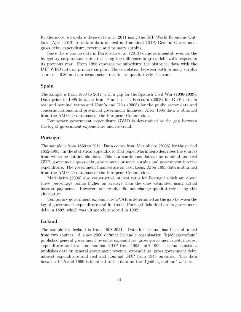
Furthermore, we update these data until 2011 using the IMF World Economic Out-look (April 2012) to obtain data on real and nominal GDP, General Governmentgross debt, expenditure, revenue and primary surplus.

Since there was no data in Bartoletto et al. (2013) on governmental revenue, thebudgetary surplus was estimated using the difference in gross debt with respect toits previous year. From 1988 onwards we substitute the historical data with theIMF WEO data on primary surplus. The correlation between both primary surplussources is 0.86 and our econometric results are qualitatively the same.

Spain

The sample is from 1850 to 2011 with a gap for the Spanish Civil War (1936-1939).Data prior to 1995 is taken from Prados de la Escosura (2003) for GDP data inreal and nominal terms and Comín and Díaz (2005) for the public sector data andconcerns national and provincial government finances. After 1995 data is obtainedfrom the AMECO database of the European Commission.

Temporary government expenditure GVAR is determined as the gap betweenthe log of government expenditure and its trend.

Portugal

The sample is from 1850 to 2011. Data comes from Marinheiro (2006) for the period1852-1995. In the statistical appendix to that paper Marinheiro describes the sourcesfrom which he obtains his data. This is a continuous dataset on nominal and realGDP, government gross debt, government primary surplus and government interestexpenditure. The government finances are on cash basis. After 1995 data is obtainedfrom the AMECO database of the European Commission.

Marinheiro (2006) also constructed interest rates for Portugal which are aboutthree percentage points higher on average than the ones estimated using actualinterest payments. However, our results did not change qualitatively using thisalternative.

Temporary government expenditure GVAR is determined as the gap between thelog of government expenditure and its trend. Portugal defaulted on its governmentdebt in 1892, which was ultimately resolved in 1902.

Iceland

The sample for Iceland is from 1908-2011. Data for Iceland has been obtainedfrom two sources. A since 2000 defunct Icelandic organisation "Þjóðhagsstofnun"published general government revenue, expenditure, gross government debt, interestexpenditure and real and nominal GDP from 1908 until 1999. Iceland statisticspublishes data on general government revenue, expenditure, gross government debt,interest expenditure and real and nominal GDP from 1945 onwards. The databetween 1945 and 1999 is identical to the data on the "Þjóðhagsstofnun" website.

44

Icelandic data concerns general government and contains long periods of highinflation. Temporary government expenditure GVAR is determined as the gap be-tween the log of government expenditure and its trend. Iceland sought and receivedassistance from the IMF and the Scandinavian countries after the 2008 banking cri-sis turned into a sovereign debt crisis for Iceland. This is considered as a public debtdefault.

45

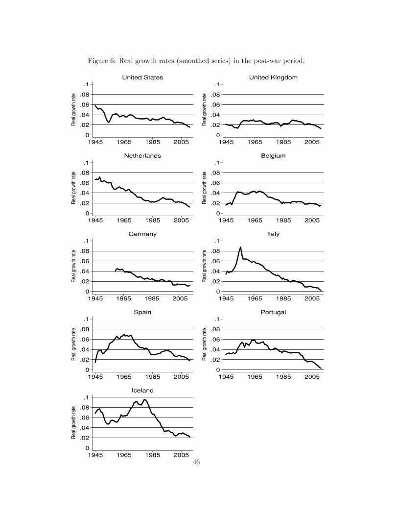
Figure 6: Real growth rates (smoothed series) in the post-war period.

0

.02

.04

.06

.08

.1

Rea

l gro

wth

rat

e

1945 1965 1985 2005

United States

0

.02

.04

.06

.08

.1

Rea

l gro

wth

rat

e

1945 1965 1985 2005

United Kingdom

0

.02

.04

.06

.08

.1

Rea

l gro

wth

rat

e

1945 1965 1985 2005

Netherlands

0

.02

.04

.06

.08

.1

Rea

l gro

wth

rat

e

1945 1965 1985 2005

Belgium

0

.02

.04

.06

.08

.1

Rea

l gro

wth

rat

e

1945 1965 1985 2005

Germany

0

.02

.04

.06

.08

.1

Rea

l gro

wth

rat

e

1945 1965 1985 2005

Italy

0

.02

.04

.06

.08

.1

Rea

l gro

wth

rat

e

1945 1965 1985 2005

Spain

0

.02

.04

.06

.08

.1

Rea

l gro

wth

rat

e

1945 1965 1985 2005

Portugal

0

.02

.04

.06

.08

.1

Rea

l gro

wth

rat

e

1945 1965 1985 2005

Iceland

46

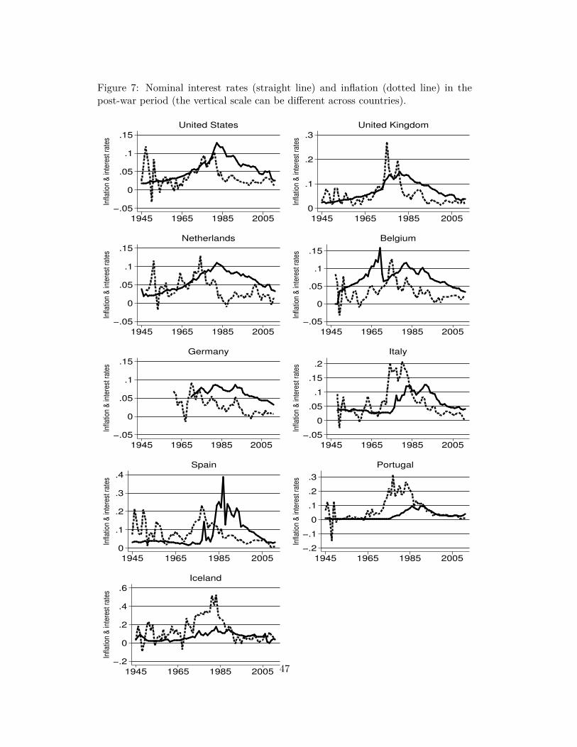
Figure 7: Nominal interest rates (straight line) and inflation (dotted line) in thepost-war period (the vertical scale can be different across countries).

−.05

0

.05

.1

.15

Infla

tio

n &

in

tere

st

rate

s

1945 1965 1985 2005

United States

0

.1

.2

.3

Infla

tion

& in

tere

st r

ates

1945 1965 1985 2005

United Kingdom

−.05

0

.05

.1

.15

Infla

tio

n &

in

tere

st

rate

s

1945 1965 1985 2005

Netherlands

−.05

0

.05

.1

.15

Infla

tion

& in

tere

st r

ates

1945 1965 1985 2005

Belgium

−.05

0

.05

.1

.15

Infla

tion

& in

tere

st r

ates

1945 1965 1985 2005

Germany

−.05

0

.05

.1

.15

.2

Infla

tion

& in

tere

st r

ates

1945 1965 1985 2005

Italy

0

.1

.2

.3

.4

Infla

tion

& in

tere

st r

ates

1945 1965 1985 2005

Spain

−.2

−.1

0

.1

.2

.3

Infla

tion

& in

tere

st r

ates

1945 1965 1985 2005

Portugal

−.2

0

.2

.4

.6

Infla

tio

n &

in

tere

st

rate

s

1945 1965 1985 2005

Iceland

47

Figure 8: United States and United Kingdom: Debt, primary surplus and militaryexpenditure ratios to GDP, and gamma parameter, post-war samples

0

.3

.6

.9

1.2

Debt / G

DP

1945 1965 1985 2005

United States

0

.5

1

1.5

2

2.5

Debt / G

DP

1945 1965 1985 2005

United Kingdom

−.1

−.05

0

.05

.1

Prim

ary

surp

lus / G

DP

1945 1965 1985 2005

United States

−.1

−.05

0

.05

.1

Prim

ary

surp

lus / G

DP

1945 1965 1985 2005

United Kingdom

.92

.94

.96

.98

1

1.02

Gam

ma

1945 1965 1985 2005

United States

.96

.98

1

1.02

1.04

Gam

ma

1945 1965 1985 2005

United Kingdom

0

.1

.2

.3

.4

Mili

tary

expenditure

/ G

DP

1945 1965 1985 2005

United States

0

.1

.2

.3

.4

.5

Mili

tary

expenditure

/ G

DP

1945 1965 1985 2005

United Kingdom

Notes: Gamma is one plus the smoothed series of the effective interest rates minus the smoothedseries of nominal GDP growth rates.

48

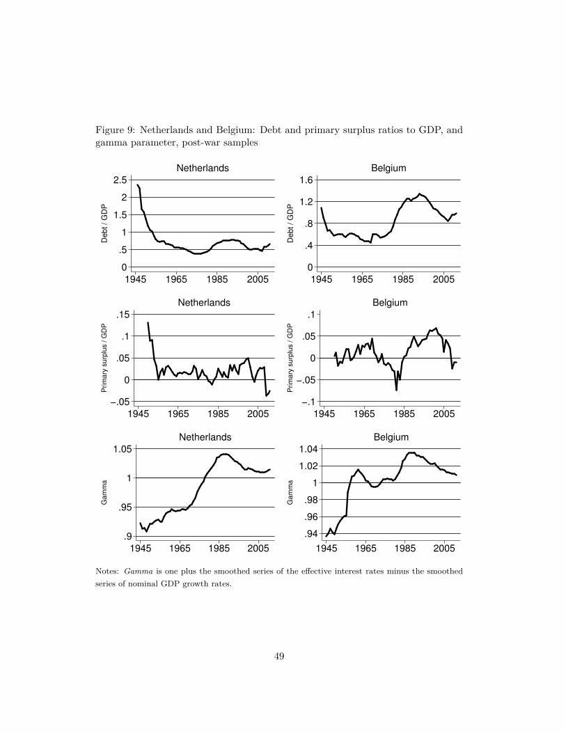
Figure 9: Netherlands and Belgium: Debt and primary surplus ratios to GDP, andgamma parameter, post-war samples

0

.5

1

1.5

2

2.5

Debt / G

DP

1945 1965 1985 2005

Netherlands

0

.4

.8

1.2

1.6

Debt / G

DP

1945 1965 1985 2005

Belgium

−.05

0

.05

.1

.15

Prim

ary

surp

lus / G

DP

1945 1965 1985 2005

Netherlands

−.1

−.05

0

.05

.1

Prim

ary

surp

lus / G

DP

1945 1965 1985 2005

Belgium

.9

.95

1

1.05

Gam

ma

1945 1965 1985 2005

Netherlands

.94

.96

.98

1

1.02

1.04

Gam

ma

1945 1965 1985 2005

Belgium

Notes: Gamma is one plus the smoothed series of the effective interest rates minus the smoothedseries of nominal GDP growth rates.

49

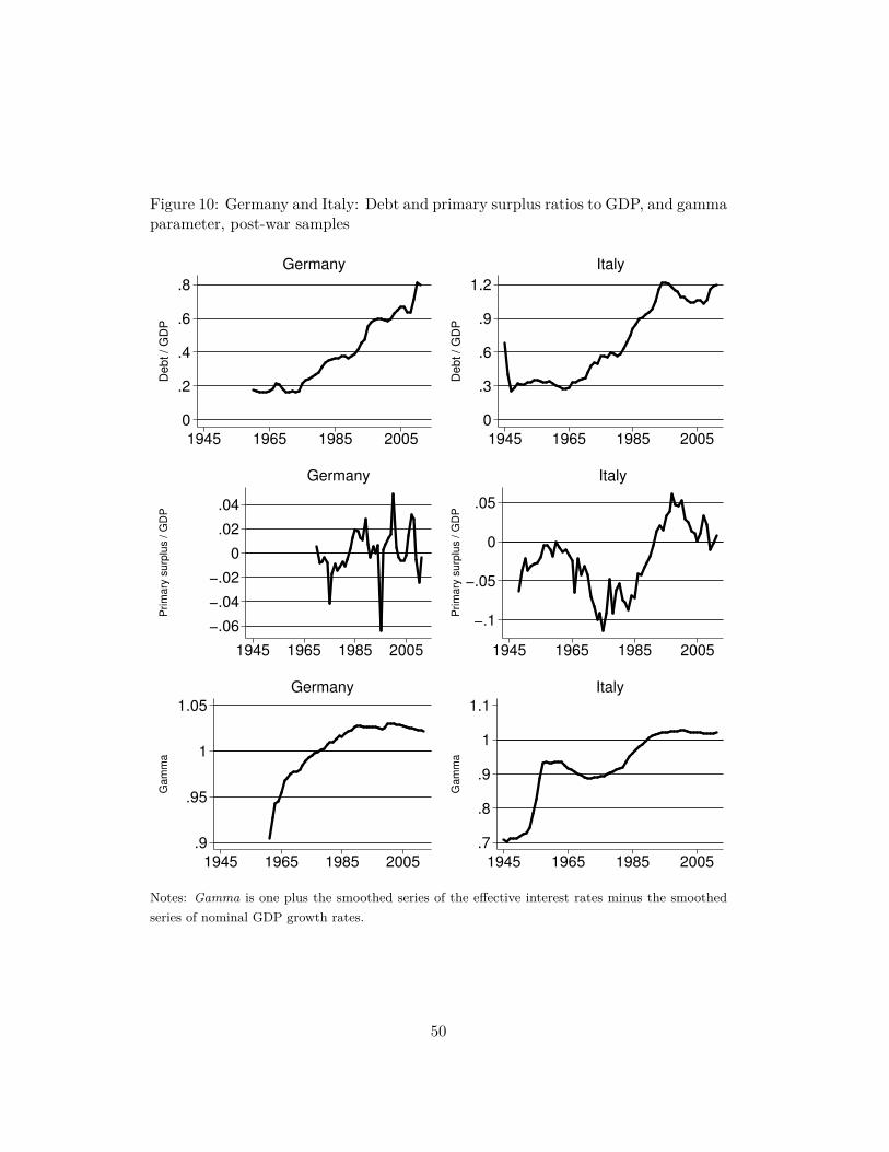
Figure 10: Germany and Italy: Debt and primary surplus ratios to GDP, and gammaparameter, post-war samples

0

.2

.4

.6

.8

Debt / G

DP

1945 1965 1985 2005

Germany

0

.3

.6

.9

1.2

Debt / G

DP

1945 1965 1985 2005

Italy

−.06

−.04

−.02

0

.02

.04

Prim

ary

surp

lus / G

DP

1945 1965 1985 2005

Germany

−.1

−.05

0

.05

Prim

ary

surp

lus / G

DP

1945 1965 1985 2005

Italy

.9

.95

1

1.05

Gam

ma

1945 1965 1985 2005

Germany

.7

.8

.9

1

1.1

Gam

ma

1945 1965 1985 2005

Italy

Notes: Gamma is one plus the smoothed series of the effective interest rates minus the smoothedseries of nominal GDP growth rates.

50

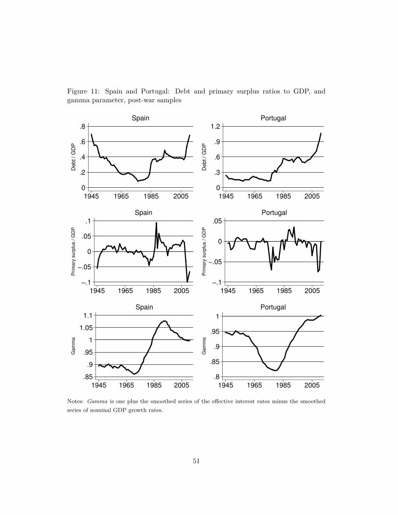
Figure 11: Spain and Portugal: Debt and primary surplus ratios to GDP, andgamma parameter, post-war samples

0

.2

.4

.6

.8

Debt / G

DP

1945 1965 1985 2005

Spain

0

.3

.6

.9

1.2

Debt / G

DP

1945 1965 1985 2005

Portugal

−.1

−.05

0

.05

.1

Prim

ary

surp

lus / G

DP

1945 1965 1985 2005

Spain

−.1

−.05

0

.05

Prim

ary

surp

lus / G

DP

1945 1965 1985 2005

Portugal

.85

.9

.95

1

1.05

1.1

Gam

ma

1945 1965 1985 2005

Spain

.8

.85

.9

.95

1

Gam

ma

1945 1965 1985 2005

Portugal

Notes: Gamma is one plus the smoothed series of the effective interest rates minus the smoothedseries of nominal GDP growth rates.

51

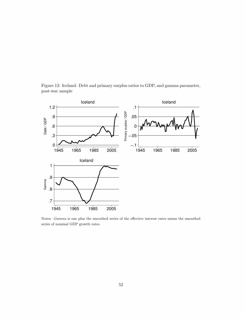
Figure 12: Iceland: Debt and primary surplus ratios to GDP, and gamma parameter,post-war sample

0

.3

.6

.9

1.2

Debt / G

DP

1945 1965 1985 2005

Iceland

−.1

−.05

0

.05

.1

Prim

ary

surp

lus / G

DP

1945 1965 1985 2005

Iceland

.7

.8

.9

1

Gam

ma

1945 1965 1985 2005

Iceland

Notes: Gamma is one plus the smoothed series of the effective interest rates minus the smoothedseries of nominal GDP growth rates.

52