A stochastic model for order book dynamicsww2040/orderbook.pdfA stochastic model for order book dynamics Rama Cont, Sasha Stoikov, Rishi Talreja IEOR Dept, Columbia University, New

A stochastic model for order book dynamicsRama Cont, Sasha Stoikov, Rishi Talreja

IEOR Dept, Columbia University, New [email protected], [email protected], [email protected]

We propose a stochastic model for the continuous-time dynamics of a limit order book. The model strikesa balance between two desirable features: it captures key empirical properties of order book dynamics andits analytical tractability allows for fast computation of various quantities of interest without resorting tosimulation. We describe a simple parameter estimation procedure based on high-frequency observations ofthe order book and illustrate the results on data from the Tokyo stock exchange. Using Laplace transformmethods, we are able to efficiently compute probabilities of various events, conditional on the state of theorder book: an increase in the mid-price, execution of an order at the bid before the ask quote moves, andexecution of both a buy and a sell order at the best quotes before the price moves. Comparison with high-frequency data shows that our model can capture accurately the short term dynamics of the limit orderbook.

Key words : Limit order book, financial engineering, Laplace transform inversion, queueing systems,simulation.

1

Cont, Stoikov and Talreja: A stochastic model for order book dynamics2

Contents

1 Introduction 3

2 A continuous-time model for a stylized limit order book 42.1 Limit order books . . . . . . . . . . . . . . . . . . . . . . . . . . . . . . . . . . . . . 42.2 Dynamics of the order book . . . . . . . . . . . . . . . . . . . . . . . . . . . . . . . . 5

3 Parameter estimation 63.1 Description of the data set . . . . . . . . . . . . . . . . . . . . . . . . . . . . . . . . . 63.2 Estimation procedure . . . . . . . . . . . . . . . . . . . . . . . . . . . . . . . . . . . 7

4 Laplace transform methods for computing conditional probabilities 84.1 Laplace transforms and first-passage times of birth-death processes . . . . . . . . . . 94.2 Direction of price moves . . . . . . . . . . . . . . . . . . . . . . . . . . . . . . . . . . 104.3 Executing an order before the mid-price moves . . . . . . . . . . . . . . . . . . . . . 124.4 Making the spread . . . . . . . . . . . . . . . . . . . . . . . . . . . . . . . . . . . . . 13

5 Numerical Results 155.1 Long term behavior . . . . . . . . . . . . . . . . . . . . . . . . . . . . . . . . . . . . 15

5.1.1 Steady state shape of the book . . . . . . . . . . . . . . . . . . . . . . . . . . 155.1.2 Volatility . . . . . . . . . . . . . . . . . . . . . . . . . . . . . . . . . . . . . . 15

5.2 Conditional distributions . . . . . . . . . . . . . . . . . . . . . . . . . . . . . . . . . 165.2.1 One-step transition probabilities . . . . . . . . . . . . . . . . . . . . . . . . . 165.2.2 Direction of price moves . . . . . . . . . . . . . . . . . . . . . . . . . . . . . . 175.2.3 Executing an order before the mid-price moves . . . . . . . . . . . . . . . . . 185.2.4 Making the spread . . . . . . . . . . . . . . . . . . . . . . . . . . . . . . . . . 18

6 Conclusion 18


1. Introduction

The evolution of prices in financial markets results from the interaction of buy and sell ordersthrough a rather complex dynamic process. Studies of the mechanisms involved in trading financialassets have traditionally focused on quote-driven markets, where a market maker or dealer central-izes buy and sell orders and provides liquidity by setting bid and ask quotes. The NYSE specialistsystem is an example of this mechanism. In recent years, Electronic Communications Networks(ECN’s) such as Archipelago, Instinet, Brut and Tradebook have captured a large share of theorder flow by providing an alternative order-driven trading system. These electronic platformsaggregate all outstanding limit orders in a limit order book that is available to market participantsand market orders are executed against the best available prices. As a result of the ECN’s popular-ity, established exchanges such as the NYSE, Nasdaq, the Tokyo Stock Exchange and the LondonStock Exchange have adopted electronic order-driven platforms, either fully or partially through“hybrid” systems.

The absence of a centralized market maker, the mechanical nature of execution of orders and–last but not least– the availability of data have made order-driven markets interesting candidatesfor stochastic modelling . At a fundamental level, models of order book dynamics may providesome insight into the interplay between order flow, liquidity and price dynamics Bouchaud et al.(2002), Smith et al. (2003), Farmer et al. (2004), Foucault et al. (2005). At the level of applications,such models provide a quantitative framework for investors and trading desks to optimize tradeexecution strategies Alfonsi et al. (2007), Obizhaeva and Wang (2006). An important motivationfor modelling high-frequency dynamics of order books is to use the information on the currentstate of the order book to predict its short-term behavior. The focus is therefore on conditionalprobabilities of events, given the state of the order book.

The dynamics of a limit order book resembles in many aspects that of a queuing system. Limitorders wait in a queue to be executed against market orders (or canceled). Drawing inspirationfrom this analogy, we model a limit order book as a continuous-time Markov process that tracks thenumber of limit orders at each price level in the book. The model strikes a balance between threedesirable features: it can be easily calibrated to high-frequency data, reproduces various empiricalfeatures of order books and is analytically tractable. In particular, we show that our model issimple enough to allow the use of Laplace transform techniques from the queueing literature tocompute various conditional probabilities. These include the probability of the mid-price increasingin the next move, the probability of executing an order at the bid before the ask quote moves andthe probability of executing both a buy and a sell order at the best quotes before the price moves,given the state of the order book. We illustrate these computations in a model estimated fromorder book data for a stock on the Tokyo stock exchange.

Related literature. Various recent studies have focused on limit order books. Given the com-plexity of the structure and dynamics of order books, it has been difficult to construct modelsthat are both statistically realistic and amenable to rigorous quantitative analysis. Parlour (1998)and Foucault et al. (2005), Rosu (forthcoming) propose equilibrium models of limit order books.These models provide interesting insights into the price formation process but contain unobserv-able parameters that govern agent preferences. Thus, they are difficult to estimate and use inapplications. Some empirical studies on properties of limit order books are Bouchaud et al. (2002),Farmer et al. (2004), and Hollifield et al. (2004). These studies provide an extensive list of sta-tistical features of order book dynamics which are challenging to incorporate in a single model.Bouchaud et al. (2008), Smith et al. (2003), Bovier et al. (2006), Luckock (2003), and Maslov andMills (2001) propose stochastic models of order book dynamics in the spirit of the one proposedhere but focus on unconditional / steady–state distributions of various quantities rather than theconditional quantities we focus on here.


The model proposed here is admittedly simpler in structure than some others existing in theliterature: it does not incorporate strategic interaction of traders as in game theoretic approachesParlour (1998), Foucault et al. (2005) and Rosu (forthcoming), nor does it account for “longmemory” features of the order flow as pointed out by Bouchaud et al. (2002) and Bouchaud et al.(2008). However, contrarily to these models, it leads to an analytically tractable framework whereparameters can be easily estimated from empirical data and various quantities of interest may becomputed efficiently.

Outline. The paper is organized as follows. §2 describes a stylized model for the dynamics ofa limit order book, where the order flow is described by independent Poisson processes. Estima-tion of model parameters from high-frequency order book time series data is described in §3 andillustrated using data from the Tokyo Stock Exchange. In §4 we show how this model can be usedto compute conditional probabilities of various types of events relevant for trade execution usingLaplace transform methods. §5 explores steady state properties of the model using Monte Carlosimulation and compares conditional probabilities computed by simulation to those computed withthe Laplace transform methods presented in §4.

2. A continuous-time model for a stylized limit order book

2.1. Limit order books

Consider a financial asset traded in an order-driven market. Market participants can post two typesof buy/sell orders. A limit order is an order to trade a certain amount of a security at a given price.Limit orders are posted to a electronic trading system and the state of outstanding limit orderscan be summarized by stating the quantities posted at each price level: this is known as the limitorder book. The lowest price for which there is an outstanding limit sell order is called the ask priceand the highest buy price is called the bid price.

A market order is an order to buy/sell (a certain quantity of) the asset at the best availableprice in the limit order book. When a market order arrives it is matched with the best availableprice in the limit order book and a trade occurs. The quantities available in the limit order bookare updated accordingly.

A limit order sits in the order book until it is either executed against a market order or it iscanceled. A limit order may be executed very quickly if it corresponds to a price near the bid andthe ask, but may take a long time if the market price moves away from the requested price or ifthe requested price is too far from the bid/ask. Alternatively, a limit order can be canceled at anytime.

We consider a market where limit orders can be placed on a price grid {1, . . . , n} representingmultiples of a price tick. We track the state of the order book with a continuous-time processX(t) ≡ (X1(t), . . . ,Xn(t))t≥0, where |Xp(t)| is the number of outstanding limit orders at price p,1 ≤ p ≤ n. If Xp(t) < 0, then there are −Xp(t) bid orders at price p; if Xp(t) > 0, then there areXp(t) ask orders at price p.

The ask price pA(t) at time t is then defined by

pA(t) = inf{p = 1, . . . , n, Xp(t) > 0}∧ (n +1).

Similarly, the bid price pB(t) is defined by

pB(t)≡ sup{p = 1, . . . , n, Xp(t) < 0, }∨ 0

Notice that when there are no ask orders in the book we force an ask price of n+1 and when thereare no bid orders in the book we force a bid price of 0. The mid-price pM (t) and the bid-ask spreads(t) are defined by

pM(t)≡ pB(t) + pA(t)2

and s(t)≡ pA(t)− pB(t).


Since most of the trading activity takes place in the vicinity of the bid and ask prices, it is usefulto keep track of the number of outstanding orders at a given distance from the bid/ask. To thisend, we define

QBi (t) =

{XpA(t)−i(t) 0 < i < pA(t)0 pA(t)≤ i < n,

(1)

the number of buy orders at a distance i from the ask and

QAi (t) =

{XpB(t)+i(t) 0 < i < n− pB(t)0 n− pB(t)≤ i < n,

(2)

the number of sell orders at a distance i from the bid. Although X(t) and (pA(t), pB(t),QA(t),QB(t))contain the same information, the second representation highlights the shape or depth of the bookrelative to the best quotes.

2.2. Dynamics of the order book

Let us now describe how the limit order book is updated by the inflow of new orders. For a statex∈Z

n and 1≤ p≤ n, definexp±1 ≡ x± (0, . . . ,1, . . . ,0),

where the 1 in the vector on the right-hand side is in the p-th component. Assuming that allorders are of unit size (in empirical examples we will take this unit to be the average size of limitorders observed for the asset),

• a limit buy order at price level p < pA(t) increases the quantity at level p: x→ xp−1

• a limit sell order at price level p > pB(t) increases the quantity at level p: x→ xp+1

• a market buy order decreases the quantity at the ask price: x→ xpA(t)−1

• a market sell order decreases the quantity at the bid price: x→ xpB(t)+1

• a cancellation of an oustanding limit buy order at price level p < pA(t) decreases the quantityat level p: x→ xp+1

• a cancellation of an oustanding limit sell order at price level p > pB(t) decreases the quantityat level p: x→ xp−1

The evolution of the order book is thus driven by the incoming flow of market orders, limit ordersand cancellations at each price level, each of which can be represented as a counting process. Itis empirically observed Bouchaud et al. (2002) that incoming orders arrive more frequently in thevicinity of the current bid/ask price and the rate of arrival of these orders depends on the distanceto the bid/ask.

To capture these empirical features in a model that is analytically tractable and allows tocompute quantities of interest in applications –most notably conditional probabilities of variousevents– we propose a stochastic model where the events outlined above are modelled usingindependent Poisson processes. More precisely, we assume that, for i≥ 1,

• Limit buy (resp. sell) orders arrive at a distance of i ticks from the opposite best quote atindependent, exponential times with rate λ(i),

• Market buy (resp. sell) orders arrive at independent, exponential times with rate μ,• Cancellations of limit orders at a distance of i ticks from the opposite best quote occur at a

rate proportional to the number of outstanding orders: if the number of outstanding orders at thatlevel is x then the cancellation rate is θ(i)x. This assumption can be understood as follows: if wehave a batch of x outstanding orders, each of which can be canceled at an exponential time withparameter θ(i), then the overall cancellation rate for the batch is θ(i)x.


• The above events are mutually independent.

Typically, the arrival rates λ : {1, . . . , n}→ [0,∞) are decreasing functions of the distance to thebid/ask: most orders are placed close to the current price. Empirical studies suggest a power law

λ(i) =k

iα

as a plausible specification (see Zovko and Farmer (2002) or Bouchaud et al. (2002)).Given the above assumptions, X is a continuous-time Markov chain with state space Z

n andtransition rates given by

x→ xp−1 with rate λ(pA(t)− p) for p < pA(t),x→ xp+1 with rate λ(p− pB(t)) for p > pB(t),x→ xpB(t)+1 with rate μx→ xpA(t)−1 with rate μx→ xp+1 with rate θ(pA(t)− p)|xp| for p < pA(t),x→ xp−1 with rate θ(p− pB(t))|xp| for p > pB(t),

Proposition 1 X is an ergodic Markov process. In particular, X has a proper stationary distri-bution.

Proof. Define N ≡ (N(t), t ≥ 0), where N(t)≡∑n

i=1 |Xi(t)|. Then X(t) = (0, . . . ,0) if and onlyif N(t) = 0. But N is simply a birth-death process with birth rate bounded from above by λ ≡2∑n

i=0 λ(i) and death rate in state i, μi ≡ 2μ+ iθ. Then, we have the inequalities∞∑

i=1

λi

μ1 · · ·μi

<∞∑

i=1

1i!

(λ

θ

)i

= eλθ − 1 <∞,

and ∞∑i=1

μ1 · · ·μi

λi>

M∑i=1

μ1 · · ·μi

λi+

∞∑i=M+1

(2μ+Mθ

λ

)i

=∞,

for M > 0 chosen large enough so that 2μ+Mθ > λ. Therefore, by (Asmussen 2003, Corollary 2.5)the birth-death process is ergodic. Since X is clearly irreducible, it follows that X is also ergodic.

�The ergodicity of X is a desirable feature: it allows to compare time averages of various quantities

(average shape of the order book, average price impact, etc.) to expectations of these quantitiescomputed in the model. The steady-state behavior of X will be further discussed in §5.1.

3. Parameter estimation

3.1. Description of the data set

Our data consists of time-stamped sequences of trades (market orders) and quotes (prices, quan-tities of outstanding limit orders) for the 5 best price levels on each side of the order book, forstocks traded on the Tokyo stock exchange. This data set, referred to as Level II order book data,provides a more detailed view of price dynamics than the Trade and Quotes (TAQ) data often usedfor high frequency data analysis, which consist of prices and sizes of trades (market orders) andtime-stamped updates in the price and size of the bid and ask quotes.

In Table 1, we display a sample of three consecutive trades for Sky Perfect Communications.Each row provides the time, size and price of a market order. We also display a sample of Level IIbid side quotes. Each row displays the 5 bid prices (pb1, pb2, pb3, pb4 and pb5), as well as thequantity of shares bid at these respective prices (qb1, qb2, qb3, qb4, qb5).


time price size9:11:01 74300 19:11:04 74600 29:11:19 74400 1

time pb1 pb2 pb3 pb4 pb5 qb1 qb2 qb3 qb4 qb59:11:01 74300 74200 74000 73900 73800 12 13 1 52 119:11:03 74400 74300 74200 74000 73900 20 12 13 1 529:11:04 74400 74300 74200 74000 73900 21 11 13 1 529:11:05 74400 74300 74200 74000 73900 34 4 13 1 529:11:19 74400 74300 74200 74000 73900 33 4 13 1 52

Table 1 A sample of 3 trades and 5 quotes for Sky Perfect Communications

3.2. Estimation procedure

Recall that in our stylized model we assume orders to be of unit size. In the data set, we firstcompute the average size of market orders Sm, of limit orders Sl and of canceled orders Sc andchoose the size unit to be the average size of a limit order Sl: a block of orders of size Sl is countedas one event. The limit order arrival rate function for 1≤ i≤ 5 can be estimated by

λ(i) =Nl(i)

T,

where Nl(i) is the total number of limit orders that arrived at a distance i from the opposite bestquote. Nl(i) is obtained by enumerating the number of times that a quote increases in size at adistance of 1 ≤ i ≤ 5 ticks from the opposite best quote. We then extrapolate by fitting a powerlaw function of the form

λ(i) =k

iα

(suggested by Zovko and Farmer (2002) or Bouchaud et al. (2002)). The power law parameters kand α are obtained by a least squares fit

mink,α

5∑i=1

(λ(i)− k

iα

)2

.

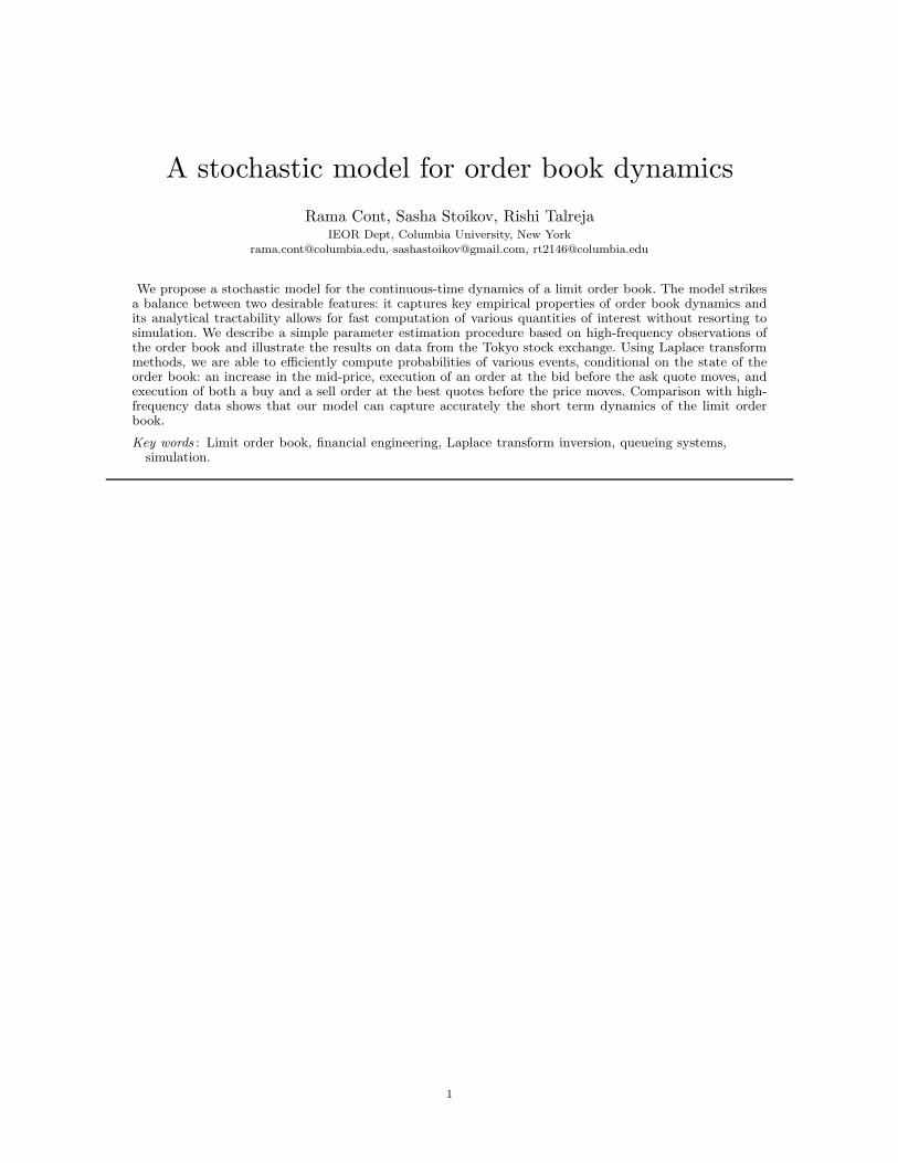
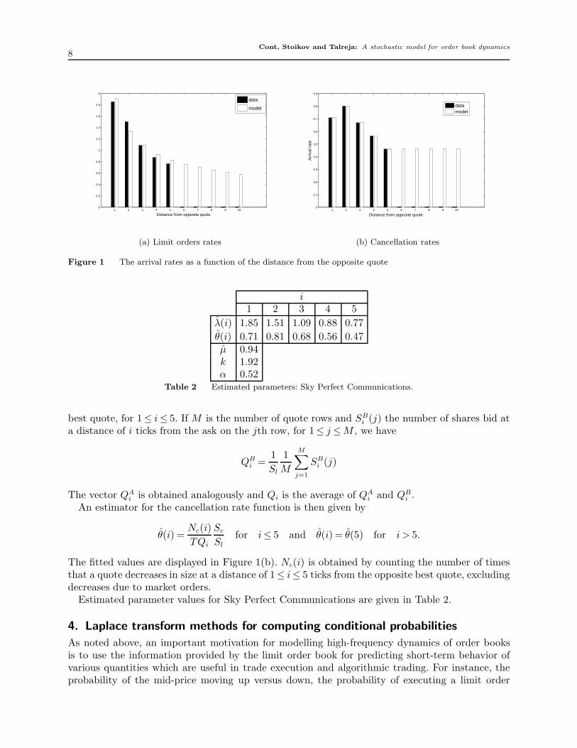
Estimated arrival rates at distances 0≤ i≤ 10 from the opposite best quote are displayed in Figure1(a).

The arrival rate of market orders is then estimated by

μ =Nm

T

Sm

Sl

,

where T is the length of our sample (in minutes) and Nm is the number of market orders. Notethat we ignore market orders that do not affect the best quotes, as is the case when a market orderis matched by a hidden or ‘iceberg’ order.

Since the cancellation rate in our model is proportional to the number of orders at a particularprice level, in order to estimate cancellation rate we first need to estimate the steady state shape ofthe order book Qi, which is the average number of orders at a distance of i ticks from the opposite


1 2 3 4 5 6 7 8 9 100

0.2

0.4

0.6

0.8

1

1.2

1.4

1.6

1.8

2

Distance from opposite quote

data

model

(a) Limit orders rates

1 2 3 4 5 6 7 8 9 100

0.1

0.2

0.3

0.4

0.5

0.6

0.7

0.8

0.9

Distance from opposite quote

Arr

ival

rat

e

datamodel

(b) Cancellation rates

Figure 1 The arrival rates as a function of the distance from the opposite quote

i1 2 3 4 5

λ(i) 1.85 1.51 1.09 0.88 0.77θ(i) 0.71 0.81 0.68 0.56 0.47μ 0.94k 1.92α 0.52

Table 2 Estimated parameters: Sky Perfect Communications.

best quote, for 1≤ i≤ 5. If M is the number of quote rows and SBi (j) the number of shares bid at

a distance of i ticks from the ask on the jth row, for 1≤ j ≤M , we have

QBi =

1Sl

1M

M∑j=1

SBi (j)

The vector QAi is obtained analogously and Qi is the average of QA

i and QBi .

An estimator for the cancellation rate function is then given by

θ(i) =Nc(i)TQi

Sc

Sl

for i≤ 5 and θ(i) = θ(5) for i > 5.

The fitted values are displayed in Figure 1(b). Nc(i) is obtained by counting the number of timesthat a quote decreases in size at a distance of 1≤ i≤ 5 ticks from the opposite best quote, excludingdecreases due to market orders.

Estimated parameter values for Sky Perfect Communications are given in Table 2.

4. Laplace transform methods for computing conditional probabilities

As noted above, an important motivation for modelling high-frequency dynamics of order booksis to use the information provided by the limit order book for predicting short-term behavior ofvarious quantities which are useful in trade execution and algorithmic trading. For instance, theprobability of the mid-price moving up versus down, the probability of executing a limit order


at the bid before the ask quote moves and the probability of executing both a buy and a sellorder at the best quotes before the price moves. These quantities can be expressed in terms ofconditional probabilities of events, given the state of the order book. In this section we show thatthe model proposed in §2 allows such conditional probabilities to be analytically computed usingLaplace methods. After presenting some background on Laplace transforms in §4.1, we give variousexamples of these computations. The probability of an increase in the mid-price is discussed in§4.2, the probability that a limit order executes before the price moves is discussed in §4.3 andthe probability of executing both a buy and a sell limit order before the price moves is discussedin §4.4. Laplace transform methods allow efficient computation of these quantities, bypassing theneed for Monte Carlo simulation.

4.1. Laplace transforms and first-passage times of birth-death processes

We first recall some basic facts about two-sided Laplace transforms and discuss the computationof Laplace transforms for first-passage times of birth-death processes (Abate and Whitt (1999)).Given a function f : R→R, its two-sided Laplace transform is given by

f(s) =∫ ∞

−∞e−stf(t)dt,

where s is a complex numbers. When f is the probability density function (pdf) of some randomvariable X, its two-sided Laplace transform can also be written as

f(s) = E[e−sX ].

In this case, we also say that f is the two-sided Laplace transform of the random variable itself. Wework with two-sided Laplace transforms here because for our purposes the function f will usuallycorrespond to the pdf of a random variable with both positive and negative support. From nowon, we drop the prefix “two-sided” when referring to two-sided Laplace transforms. When we sayconditional Laplace-transform of the random variable X conditional on the event A, we mean theLaplace transform of the conditional pdf of X given A.

Recall that if X and Y are independent random variables with well-defined Laplace transforms,then

fX+Y (s) = E[e−s(X+Y )] = E[e−sX ]E[e−sY ] = fX(s)fY (s). (3)

If for some γ ∈ R we have∫∞−∞ |f(σ + iω)|dω < ∞ and f(t) is continuous at t, then the inverse

transform is given by the Bromwich contour integral

f(t) =1

2πi

∫ σ+i∞

σ−i∞etsf(s)ds. (4)

The continued fraction associated with a sequence {an, n≥ 1} of partial numerators and {bn, n≥1} of partial denominators, which are complex numbers with an = 0 for all n ≥ 1, is the sequence{wn, n≥ 1}, where

wn = t1 ◦ t2 ◦ · · · ◦ tn(0), n≥ 1, tk(u) =ak

bk +u, k ≥ 1.

If w ≡ limn→∞ wn, then the continued fraction is said to be convergent and the limit w is said tobe the value of the continued fraction (Abate and Whitt (1999)). In this case, we write

w ≡Φ∞n=1

an

bn

.


Consider now a birth-death process with constant birth rate λ and death rates μi in state i ≥ 1,and let σb denote the first-passage time of this process to 0 given it begins in state b. Next, noticethat we can write σB as the sum

σb = σb,b−1 +σb−1,b−2 + · · ·+σ1,0,

where σi,i−1 denotes the first-passage time of the birth-death process from the state i to the statei−1, for i = 1, . . . , b, and all terms on the right-hand side are independent. If fb denotes the Laplacetransform of σb and fi,i−1 denotes the Laplace transform of σi,i−1, for i = 1, . . . , b, then we have by(3),

fb(s) = Πbi=1fi,i−1(s). (5)

Therefore, in order to compute fb, it suffices to compute the simpler Laplace transforms fi,i−1, fori = 1, . . . , b. By Equation (4.9) of Abate and Whitt (1999), we see that the Laplace transform offi,i−1 is given by

fi,i−1(s) =− 1λ

Φ∞k=i

−λμk

λ+μk + s. (6)

The computation there is based on a recursive relationship between the fi,i−1, i = 1, . . . , b, whichis derived by considering the first transition of the birth-death process. Combining (5) and (6), weobtain

fb(s) =(− 1

λ

)b(Πb

i=1Φ∞k=i

−λμk

λ+μk + s

). (7)

We will use this result in all our computations below.

4.2. Direction of price moves

We now compute the probability that the mid-price increases at its next move. The first move inthe mid-price occurs at the first-passage time of the bid or ask queue to zero or, if the bid/askspread is greater than one, the first time a limit order arrives inside the spread. Throughout thissection, let XA ≡ XpA(·)(·) and XB ≡ |XpB(·)(·)|, and let σA and σB be the first-passage times ofXA and XB to 0, respectively. Let WB ≡ {WB(t), t≥ 0} (WA ≡ {WA(t), t≥ 0}) denote the numberof orders remaining at the bid (ask) at time t of the initial XB(0) (XA(0)) orders and let εB (εA)be the first-passage time of WB (WA) to 0. Furthermore, let T be the time of the first change inmid-price:

T ≡ inf{t≥ 0, pM (t) = pM (0)}.In this subsection, we are interested in computing the conditional probability that the mid-priceincreases before decreasing:

P[pM (T ) > pM (0)|XA(0) = a,XB(0) = b, s(0) = S], (8)

where S > 0. For ease of notation, we will omit the conditioning variables in all proofs below.The idea for computing (8) is to observe that XA and XB behave as independent birth-death

processes and WA and WB behave as independent pure-death processes for t≤ T . More precisely:

Lemma 2 Let s(0) = S. Then1. There exist independent birth-death processes XA and XB with birth rate λ(S) and death rate

μ+ iθ(S) in state i≥ 1, such that for all 0≤ t≤ T , XA(t) = XA(t) and XB(t) = XB(t).2. There exist independent pure death processes WA and WB with death rate μ+iθ(S) in state i≥

1, such that for all 0≤ t≤ T , WA(t) = WA(t) and WB(t) = WB(t). Furthermore, WA is independentof XB, WB is independent of XA, WA ≤ XA and WB ≤ XB.


The conditional probability (8) can then be computed as follows:

Proposition 3 (Probability of increase in mid-price) Let fj,S be given by

fj,S(s) =(− 1

λ(S)

)j(Πb

i=1Φ∞k=i

−λ(S) (μ+ kθ(S))λ(S) +μ+ kθ(S) + s

), (9)

for j ≥ 1, and let ΛS ≡∑S−1

i=1 λ(i). Then (8) is given by the inverse Laplace transform of

Fa,b,S(s) =1s

(fb,S(s+ΛS) +

ΛS

ΛS + s(1− fb,S(s+ΛS))

)(fa,S(ΛS − s) +

ΛS

ΛS − s(1− fa,S(ΛS − s))

),

(10)evaluated at 0. When S = 1, (10) reduces to

Fa,b,1(s) =1sfa,1(s)fb,1(−s). (11)

Proof. We will first focus on the special case when S = 1 and then extend the analysis to thecase S > 1 using Lemma 4 below. Construct XA and XB as in Lemma 2. When S = 1, the pricechanges for the first time exactly when one of the two independent birth-death processes XA andXB reaches the state 0 for the first time. Both of these birth-death processes have constant birthrates λ(1) and death rates μ + iθ(1), i ≥ 1. Thus, given our initial conditions, the distribution ofT is given by the minimum of the independent first passage times σA and σB . Furthermore, thequantity (8) is given by P[σA < σB ]. By (7), the conditional Laplace transform of σA − σB giventhe initial conditions is given by fa,1(s)fb,1(−s) so that the conditional Laplace transform of thecumulative distribution function (cdf) of σA −σB is given by (11). Thus, our desired probability isgiven by the inverse Laplace transform of (11) evaluated at 0.

We now move on to the case where S > 1. Let σiA denote the first time an ask order arrives i

ticks away from the bid and σiB denote the first time a bid order arrives i ticks away from the ask,

for i = 1, . . . , S − 1. The time of the first change in mid-price is now given by

T = σA ∧σB ∧min{σiA, σi

B , i = 1, . . . , S − 1}.Notice that XA and XB are independent of the mutually independent arrival times σi

A, σiB, for

i = 1, . . . , S − 1. Also, notice that σiA and σi

B are exponentially distributed with rates λ(i) fori = 1, . . . , S−1. The first change in mid-price is an increase if there is an arrival of a limit bid orderwithin S − 1 ticks of the best ask or XA hits zero, before there is an arrival of a limit ask orderwithin S − 1 ticks of the best bid or XB hits zero. Thus, the quantity (8) can be written as

P[σA ∧σ1B ∧ . . .∧σS−1

B < σB ∧σ1A ∧ . . .∧σS−1

A ] = P[σA ∧σΣB < σB ∧σΣ

A], (12)

where σΣA and σΣ

B are independent exponential random variables both with rate ΛS . In order tocompute (12), we first need to compute the conditional Laplace transform of the minimum σB ∧σΣ

A.This is given in Lemma 4, substituting σΣ

A for Z. The conditional Laplace transform of the randomvariable σB ∧σΣ

A−σA∧σΣB can then be computed using (3) and the probability (8) can be computed

by inverting the conditional Laplace transform of the cdf of this random variable and evaluatingat 0 as in the case S = 1. �

Lemma 4 Let Z be an exponentially distributed random variable with parameter Λ. Then theLaplace transform of the random variable σB ∧Z is given by

fb(s+Λ) +Λ

Λ+ s(1− fb(s+Λ)),

where fb is given in (9).


Proof. We first compute the density fσB∧Z of the random variable σB ∧Z in terms of the densityfb of the random variable σB. Since Z is exponential with rate Λ, we have for all t≥ 0,

P[σB ∧Z < t] = 1−P[σB > t]P[Z > t] = 1− (1−FσB(t))e−Λt.

Taking derivatives with respect to t gives

fσB∧Z(t) = fb(t)e−Λt +Λ(1−Fb(t))e−Λt,

for t≥ 0, where Fb(t) is the cdf of σB. Also, fσB∧Z(t) = 0 for t < 0. The Laplace transform of σB ∧Zis thus given by

fσB∧Z(s) =∫ ∞

−∞e−stfσB∧σΣ

B(t)dt

=∫ ∞

0

e−st(fb(t)e−Λt +Λ(1−Fb(t))e−Λt

)ds

=∫ ∞

0

e−t(s+Λ)fb(t)dt+Λ∫ ∞

0

(1−Fb(t))e−t(s+Λ)dt

= fb(s+Λ) +Λ

Λ+ s

(1− fb(s+Λ)

),

where the last equality follows from integration by parts. �Proposition 3 yields a numerical procedure for computing the probability that the next change

in the mid-price will be an increase. We discuss implementation of the procedure in §5.2.3.

4.3. Executing an order before the mid-price moves

Traders who submit limit orders obtain a better price than if they had submitted a market orderbut face the risk of non-execution and the “winner’s curse”. Whereas a market order executes withcertainty, limit orders stay in the order book until either a matching order is entered or the order iscanceled. The probability that a limit order is executed before the price moves is therefore useful inquantifying the choice between a limit order and a market order. We now compute the probabilitythat an order placed at the bid price is executed before any movement in the mid-price, given thatthe order is not canceled. Our result holds for initial spread S ≡ s(0)≥ 1, but we remark that inthe case where S = 1 the probability we are interested is equal to the probability that the order isexecuted before the mid-price moves away from the desired price, given the order is not canceled.Although we focus here on an order placed at the bid price, since our model is symmetric in bidsand asks, our result also holds for orders placed at the ask price.

We introduce some new notation, which we will used in this subsection as well as the next. LetNCb (NCa) denote the event that an order that never gets canceled is placed at the bid (ask) attime 0.

Then, the probability that an order placed at the bid is executed before the mid-price moves isgiven by

P[εB < T |XB(0) = b,XA(0) = a, s(0) = S,NCb]. (13)

Proposition 5 (Probability of order execution before mid-price moves) Define fa,S(s)as in (9) and let gj,S be given by

gj,S(s) = Πji=1

μ+ θ(S)(i− 1)μ+ θ(S)(i− 1) + s

(14)


for j ≥ 1, and let ΛS ≡∑S−1

i=1 λ(i). Then the quantity (13) is given by the inverse Laplace transformof

Fa,b,S(s) =1sgb,S(s)

(fb,S(2ΛS − s) +

2ΛS

2ΛS − s(1− fb,S(2ΛS − s))

), (15)

evaluated at 0. When S = 1, (15) reduces to

Fa,b,1(s) =1sgb,1(s)fa,1(−s). (16)

Proof. Construct XA and WB using Lemma 2. Let us first consider the case S = 1. Let T′ ≡

εB ∧T denote the first time when either the process WB hits 0 or the mid-price changes. Conditionalon an infinitely patient order being placed at the bid price at time 0, T

′is the first time when either

that order gets executed or the mid-price changes. Notice that conditional on our initial conditions,εB is given by a sum of b independent exponentially distributed random variables with parametersμ+(i− 1)θ(1), for i = 1, . . . , b, and independent of XA. Thus, the conditional Laplace transform ofεB given our initial conditions is given by (14). Since, in the case S = 1 the mid-price can changebefore time εB if and only if σA < εB, the quantity (13) can be written simply as P[εB < σA]. Using(3) with the conditional Laplace transforms of εB and σA, given in (14) and (9) respectively, weobtain (16).

This analysis can be extended to the case where S > 1 just as in the proof of Proposition 3.When S > 1, our desired quantity can be written as P[εB < σA ∧ σΣ

B ∧ σΣA]. Since the conditional

distribution of σΣB ∧σΣ

A is exponential with parameter 2ΛS. As in the proof of Proposition 3, Lemma4 then yields the result. �

4.4. Making the spread

We now compute the probability that two orders, one placed at the bid price and one placed at theask price, are both executed before the mid-price moves, given that the orders are not canceled.If the probability of executing both a buy and a sell limit order before the price moves is high, astatistical arbitrage strategy can be designed by submitting limit orders at the bid and the ask andwait for both orders to execute. If both orders execute before the price moves, the strategy has paidoff the bid-ask spread: we refer to this situation as “making the spread”. Otherwise, losses may beminimized by submitting a market order and losing the bid-ask spread. We restrict attention tothe case where the initial spread is one tick: S = 1. The probability of making the spread can beexpressed as

P[max{εA, εB}< T |XB(0) = b,XA(0) = a, s(0) = 1,NCa,NCb]. (17)

The following result allows to compute this probability using Laplace transform methods:

Proposition 6 The probability (17) of making the spread is given by ha,b +hb,a, where

ha,b =∞∑

i=0

a∑j=1

P[εj < σi]∫ ∞

0

P X0,i(t)P

Wa,j(t)gb(t)dt, (18)

where

P X0,i(t) =

e−λX (t)λX(t)i

i!, λX(t)≡ λ

θ

(1− e−θt

)(19)

P Wa,j(t)≡

(eQW

a t)

a,j≡( ∞∑

k=0

tk

k!(QW

a )k

)a,j

(20)


QWa ≡

⎡⎢⎢⎢⎢⎢⎣

0 0 0 · · · 0μ −μ 0 · · · 00 μ+ θ −μ− θ · · · 0...

.... . . . . .

...0 0 · · · μ+(a− 1)θ −μ− (a− 1)θ

⎤⎥⎥⎥⎥⎥⎦ . (21)

and gb is the inverse Laplace transform of gb,1, which is given in (14).

Proof. Since S = 1, T = min{σA, σB}, and the quantity (17) can be written as

P[max{εB, εA}< min{σB , σA}]. (22)

Construct XA, XB, WA and WB using Lemma 2. Let T′= max{εA, εB} ∧ T denote the first time

when either both the processes WA and WB have hit 0 or the mid-price has changed. Conditionalon infinitely patient orders being placed at the best bid and ask prices at time 0, T

′is the first

time when either both the orders get executed or the mid-price changes. Furthermore, by Lemma2, WA and WB are independent pure death processes with death rate μ+ iθ(1) in state i≥ 1, andWA(t) ≤ XA(t) and WB(t)≤ XB(t). This implies that εA and εB are independent and σA and σB

are independent with εA ≤ σA and εB ≤ σB. Using these properties we obtain

P[max{εB , εA}< min{σB , σA}] = P[εB < σA, εA < σB]= P[εB < σA, εA < σB, εB < εA] + P[εB < σA, εA < σB , εA < εB]= P[εA < σB, εB < εA] + P[εB < σA, εA < εB ]= ha,b +hb,a (23)

where we define ha,b = P[εB < εA < σB ], the probability that the order placed at the bid is executedbefore the order placed at the ask and the order at the ask is executed before the bid quotedisappears. We now focus on computing ha,b. Conditioning on the value of εB gives

ha,b =∫ ∞

0

P[εB < εA < σB |εB = t]gb(t)dt. (24)

Focusing on the first factor in the integrand in (24) and conditioning on the values of XB(t) andWA(t) gives us

P[εB < εA < σB |εB = t] =∞∑

i=0

a∑j=0

P[εB < εA < σB |εB = t, XB(t) = i, WA(t) = j]P[XB(t) = i, WA(t) = j|εB = t]

=∞∑

i=0

a∑j=1

P[εj < σi]P[XB(t) = i|εB = t]P[WA(t) = j|εB = t]

=∞∑

i=0

a∑j=1

P[εj < σi]P[XB(t) = i|εB = t]P[WA(t) = j] (25)

Combining the equations (23)-(25) and using Tonelli’s theorem to interchange the integral and thesummation gives us

ha,b =∞∑

i=0

a∑j=1

P[εj < σi]∫ ∞

0

P[XB(t) = i|εB = t]P[WA(t) = j]gb(t)dt.

The quantity P[XB(t) = i|εB = t] can be computed using an analogy with the M/M/∞ queue.The number of orders in the bid queue at the time when the bid order placed at time 0 has executed


is simply the number of customers in an initially empty M/M/∞ queue with arrival rate λ andservice rate θ, which has a Poisson distribution with mean given by (19). This remark leads to(??).

The quantity P[WA(t) = j] is the probability that a pure death process with death rate μ+(k−1)θ(1) in state k ≥ 1 is in state j at time t, given it begins in state a. The infinitesimal generator ofthis pure death process is given by (21). Thus, by Corollary II.3.5 of Asmussen (2003), P[WA(t) = j]is given by (20). �

5. Numerical Results

Our stochastic model allows one to compute various quantities of interest by simulating the evolu-tion of the order book and and by using the Laplace transform methods presented in §4, based onparameters μ, λ and θ estimated from the order flow. In this section we compute these quantitiesfor the example of Sky Perfect Communications and compare them to empirically observed values,in order to assess the precision of the description provided by our model.

In §5.1, we compare empirically observed long-term behavior (e.g. unconditional properties) ofthe order book to simulations of the fitted model. Although these quantities may not be particularlyimportant for traders who are interested in trading in a short time scale, they indicate how wellthe model reproduces the average properties of the order book. In §5.2, we compare conditionalprobabilities of various events in our model to frequencies of the events in the data. We also compareresults using the Laplace transform methods developed in §4 to our simulation results.

5.1. Long term behavior

Recent empirical studies on order books Bouchaud et al. (2002, 2008) have mainly focused on aver-age properties of the order book, which, in our context correspond to unconditional expectations ofquantities under the stationary measure of X: the steady state shape of the book and the volatilityof the mid-price. The ergodicity of the Markov chain X, shown in Proposition 1, implies that suchexpectations E[f(X∞)] can be computed in the model by simulating the order book over a largehorizon T and averaging f(X(t)) over the simulated path:

1T

∫ T

0

f(X(t))dt→E[f(X∞)] as T →∞.

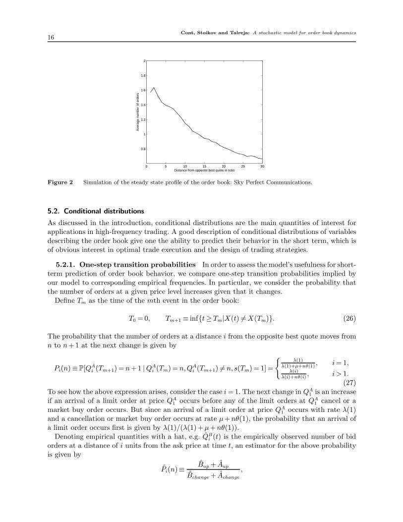
5.1.1. Steady state shape of the book We simulate the order book over a long horizon(n = 106 events) and observe the mean number of orders Qi at distances 1≤ i≤ 30 ticks from theopposite best quote. The results are displayed in Figure 2. The steady state profile of the orderbook describes the average market impact of trades Farmer et al. (2004), Bouchaud et al. (2008).Figure 2 shows that the average profile of the order book displays a hump (in this case, at twoticks from the bid/ask), as observed in empirical studies Bouchaud et al. (2008). Note that thishump feature does not result from any fine-tuning of model parameters or additional ingredients(such as correlation between order flow and past price moves).

5.1.2. Volatility Define the realized volatility of the asset over a day to be given by

RVn =

√√√√ n∑i=1

(log(

Pi+1

Pi

))2

,

where n is the number of quotes in a day and the prices Pi represent the mid-price of the stock. Inthe first day of the sample, we compute a realized volatility of 0.0219 after a total of 370 trades.After repeatedly simulating our model for 370 trades (using parameters λ, μ and θ estimatedfrom the order book time series) we obtained a 95% confidence interval for realized volatility of0.0228 ± 0.0003. Interestingly, this estimator yields the correct order of magnitude for realizedvolatility solely based on intensity parameters for the order flow (λ,μ, θ).


0 5 10 15 20 25 30

0.8

1

1.2

1.4

1.6

1.8

2

Distance from opposite best quote in ticks

Ave

rage

num

ber

of o

rder

s

Figure 2 Simulation of the steady state profile of the order book: Sky Perfect Communications.

5.2. Conditional distributions

As discussed in the introduction, conditional distributions are the main quantities of interest forapplications in high-frequency trading. A good description of conditional distributions of variablesdescribing the order book give one the ability to predict their behavior in the short term, which isof obvious interest in optimal trade execution and the design of trading strategies.

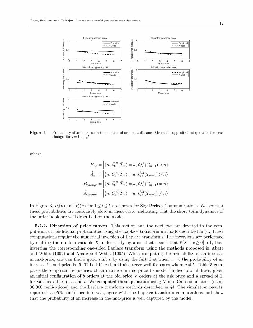
5.2.1. One-step transition probabilities In order to assess the model’s usefulness for short-term prediction of order book behavior, we compare one-step transition probabilities implied byour model to corresponding empirical frequencies. In particular, we consider the probability thatthe number of orders at a given price level increases given that it changes.

Define Tm as the time of the mth event in the order book:

T0 = 0, Tm+1 ≡ inf{t≥ Tm|X(t) = X(Tm)}. (26)

The probability that the number of orders at a distance i from the opposite best quote moves fromn to n +1 at the next change is given by

Pi(n)≡ P[QAi (Tm+1) = n +1 |QA

i (Tm) = n,QAi (Tm+1) = n, s(Tm) = 1] =

{λ(1)

λ(1)+μ+nθ(1), i = 1,

λ(i)

λ(i)+nθ(i), i > 1.

(27)To see how the above expression arises, consider the case i = 1. The next change in QA

1 is an increaseif an arrival of a limit order at price QA

1 occurs before any of the limit orders at QA1 cancel or a

market buy order occurs. But since an arrival of a limit order at price QA1 occurs with rate λ(1)

and a cancellation or market buy order occurs at rate μ+nθ(1), the probability that an arrival ofa limit order occurs first is given by λ(1)/(λ(1) +μ+nθ(1)).

Denoting empirical quantities with a hat, e.g. QBi (t) is the empirically observed number of bid

orders at a distance of i units from the ask price at time t, an estimator for the above probabilityis given by

Pi(n)≡ Bup + Aup

Bchange + Achange

,


0 1 2 3 4 5 6 70

0.5

1

Queue sizeP

roba

bilit

y of

incr

ease

1 tick from opposite quote

EmpiricalModel

0 1 2 3 4 5 6 70

0.5

1

Queue size

Pro

babi

lity

of in

crea

se

2 ticks from opposite quote

EmpiricalModel

0 1 2 3 4 5 6 70

0.5

1

Queue size

Pro

babi

lity

of in

crea

se


EmpiricalModel

0 1 2 3 4 5 6 70

0.5

1

Queue size

Pro

babi

lity

of in

crea

se


EmpiricalModel

0 1 2 3 4 5 6 70

0.5

1

Queue size

Pro

babi

lity

of in

crea

se


EmpiricalModel

Figure 3 Probability of an increase in the number of orders at distance i from the opposite best quote in the nextchange, for i = 1, . . . ,5.

where

Bup =∣∣∣{m|QB

i (Tm) = n, QBi (Tm+1) > n}

∣∣∣Aup =

∣∣∣{m|QAi (Tm) = n, QA

i (Tm+1) > n}∣∣∣

Bchange =∣∣∣{m|QB

i (Tm) = n, QBi (Tm+1) = n}

∣∣∣Achange =

∣∣∣{m|QAi (Tm) = n, QA

i (Tm+1) = n}∣∣∣

In Figure 3, Pi(n) and Pi(n) for 1≤ i≤ 5 are shown for Sky Perfect Communications. We see thatthese probabilities are reasonably close in most cases, indicating that the short-term dynamics ofthe order book are well-described by the model.

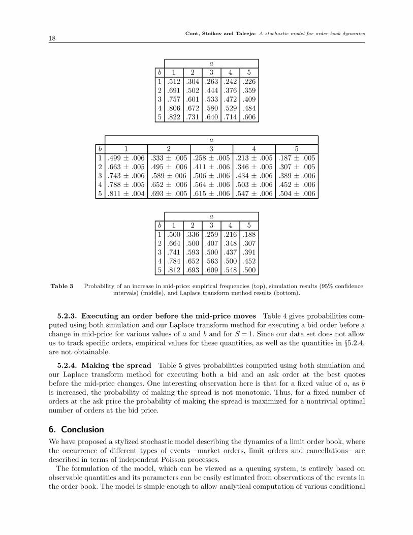
5.2.2. Direction of price moves This section and the next two are devoted to the com-putation of conditional probabilities using the Laplace transform methods described in §4. Thesecomputations require the numerical inversion of Laplace transforms. The inversions are performedby shifting the random variable X under study by a constant c such that P[X + c ≥ 0] ≈ 1, theninverting the corresponding one-sided Laplace transform using the methods proposed in Abateand Whitt (1992) and Abate and Whitt (1995). When computing the probability of an increasein mid-price, one can find a good shift c by using the fact that when a = b the probability of anincrease in mid-price is .5. This shift c should also serve well for cases where a = b. Table 3 com-pares the empirical frequencies of an increase in mid-price to model-implied probabilities, givenan initial configuration of b orders at the bid price, a orders at the ask price and a spread of 1,for various values of a and b. We computed these quantities using Monte Carlo simulation (using30,000 replications) and the Laplace transform methods described in §4. The simulation results,reported as 95% confidence intervals, agree with the Laplace transform computations and showthat the probability of an increase in the mid-price is well captured by the model.


ab 1 2 3 4 51 .512 .304 .263 .242 .2262 .691 .502 .444 .376 .3593 .757 .601 .533 .472 .4094 .806 .672 .580 .529 .4845 .822 .731 .640 .714 .606

ab 1 2 3 4 51 .499 ± .006 .333 ± .005 .258 ± .005 .213 ± .005 .187 ± .0052 .663 ± .005 .495 ± .006 .411 ± .006 .346 ± .005 .307 ± .0053 .743 ± .006 .589 ± 006 .506 ± .006 .434 ± .006 .389 ± .0064 .788 ± .005 .652 ± .006 .564 ± .006 .503 ± .006 .452 ± .0065 .811 ± .004 .693 ± .005 .615 ± .006 .547 ± .006 .504 ± .006

ab 1 2 3 4 51 .500 .336 .259 .216 .1882 .664 .500 .407 .348 .3073 .741 .593 .500 .437 .3914 .784 .652 .563 .500 .4525 .812 .693 .609 .548 .500

Table 3 Probability of an increase in mid-price: empirical frequencies (top), simulation results (95% confidenceintervals) (middle), and Laplace transform method results (bottom).

5.2.3. Executing an order before the mid-price moves Table 4 gives probabilities com-puted using both simulation and our Laplace transform method for executing a bid order before achange in mid-price for various values of a and b and for S = 1. Since our data set does not allowus to track specific orders, empirical values for these quantities, as well as the quantities in §5.2.4,are not obtainable.

5.2.4. Making the spread Table 5 gives probabilities computed using both simulation andour Laplace transform method for executing both a bid and an ask order at the best quotesbefore the mid-price changes. One interesting observation here is that for a fixed value of a, as bis increased, the probability of making the spread is not monotonic. Thus, for a fixed number oforders at the ask price the probability of making the spread is maximized for a nontrivial optimalnumber of orders at the bid price.

6. Conclusion

We have proposed a stylized stochastic model describing the dynamics of a limit order book, wherethe occurrence of different types of events –market orders, limit orders and cancellations– aredescribed in terms of independent Poisson processes.

The formulation of the model, which can be viewed as a queuing system, is entirely based onobservable quantities and its parameters can be easily estimated from observations of the events inthe order book. The model is simple enough to allow analytical computation of various conditional


ab 1 2 3 4 51 .498 ± .004 .642 ± .004 .709 ± .004 .748 ± .004 .779 ± .0042 .299 ± .004 .451 ± .004 .536 ± .004 .592 ± .004 .632 ± .0043 .204 ± .004 .335 ± .004 .422 ± .004 .484 ± .004 .532 ± .0044 .152 ± .003 .264 ± .004 .344 ± .004 .403 ± .004 .450 ± .0045 .117 ± .003 .213 ± .004 .291 ± .004 .342 ± .004 .394 ± .004

ab 1 2 3 4 51 .497 .641 .709 .749 .7762 .302 .449 .535 .591 .6313 .206 .336 .422 .483 .5284 .152 .263 .344 .404 .4525 .118 .213 .287 .346 .393

Table 4 Probability of executing a bid order before a change in mid-price: simulation results (95% confidenceintervals) (top) and Laplace transform method results (bottom).

ab 1 2 3 4 51 .268 ± .004 .306 ± .004 .312 ± .004 .301 ± .004 .286 ± .0042 .306 ± .004 .384 ± .004 .406 ± .004 .411 ± .004 .401 ± .0043 .312 ± .004 .406 ± .004 .441 ± .004 .455 ± .004 .456 ± .0044 .301 ± .004 .411 ± .004 .455 ± .004 .473 ± .004 .485 ± .0045 .286 ± .004 .401 ± .004 .456 ± .004 .485 ± .004 .491 ± .004

ab 1 2 3 4 51 .266 .308 .309 .300 .2882 .308 .386 .406 .406 .4003 .309 .406 .441 .452 .4524 .300 .406 .452 .471 .4795 .288 .400 .452 .479 .491

Table 5 Probability of making the spread: simulation results (95% confidence intervals) (top) and Laplacetransform method results (bottom).

probabilities of order book events via Laplace transform methods, yet rich enough to capture ade-quately the short-term behavior of the order book: conditional distributions of various quantitiesof interest show good agreement with the corresponding empirical distributions for parametersestimated from data sets from the Tokyo Stock Exchange. The ability of our model to computeconditional distributions is useful for short-term prediction and design of automated trading strate-gies. Finally, simulation results illustrate that our model also yields realistic features for long-term(steady state) average behavior of the order book profile and of price volatility.


One by-product of this study is to show how far a stochastic model can go in reproducing thedynamic properties of a limit order book without resorting to detailed behavioral assumptionsabout market participants or introducing unobservable parameters describing agent preferences,as in the market microstructure literature.

This model can be extended in various ways to take into account a richer set of empiricallyobserved properties Bouchaud et al. (2008). Correlation of the order flow with recent price behaviorcan be modeled by introducing state-dependent intensities of order arrivals. The heterogeneity oforder sizes, which appears to be an important ingredient, can be incorporated via a distribution oforder sizes. Both of these features conserve the Markovian nature of the process. A more realisticdistribution of inter-event times may also be introduced by modelling the event arrivals via renewalprocesses. It remains to be seen whether the analytical tractability of the model can be preservedwhen such ingredients are introduced. We look forward to exploring such extensions in a futurework.

AcknowledgmentsThe authors thank Ning Cai, Alexander Cherny, Jim Gatheral, Zongjian Liu, Peter Randolph and WardWhitt for useful discussions.

ReferencesAbate, J., W. Whitt. 1992. The Fourier-series method for inverting transforms of probability distributions.

Queueing Systems 10 5–88.

Abate, J., W. Whitt. 1995. Numerical inversion of Laplace transforms of probability distributions. ORSAJournal on Computing 7(1) 36–43.

Abate, J., W. Whitt. 1999. Computing Laplace transforms for numerical inversion via continued fractions.INFORMS Journal on Computing 11(4) 394–405.

Alfonsi, A., A. Schied, A. Schulz. 2007. Optimal execution strategies in limit order books with general shapefunctions. Working paper.

Asmussen, S. 2003. Applied Probability and Queues . Springer-Verlag.

Bouchaud, J. P., D. Farmer, F. Lillo. 2008. How markets slowly digest changes in supply and demand.Th. Hens, K. Schenk-Hoppe, eds., Handbook of Financial Markets: Dynamics and Evolution. AcademicPress.

Bouchaud, Jean-Philippe, Marc Mezard, Marc Potters. 2002. Statistical properties of stock order books:empirical results and models. Quantitative Finance 2 251–256.

Bovier, A., J. Cerny, O. Hryniv. 2006. The opinion game: Stock price evolution from microscopic marketmodelling. Int. J. Theor. Appl. Finance 9 91–111.

Farmer, J. Doyne, Laszlo Gillemot, Fabrizio Lillo, Szabolcs Mike, Anindya Sen. 2004. What really causeslarge price changes? Quantitative Finance 4 383–397.

Foucault, T., O. Kadan, E. Kandel. 2005. Limit order book as a market for liquidity. Review of FinancialStudies 18(4) 1171–1217.

Hollifield, B., R. A. Miller, P. Sandas. 2004. Empirical analysis of limit order markets. Review of EconomicStudies 71(4) 1027–1063.

Luckock, H. 2003. A steady-state model of the continuous double auction. Quantitative Finance 3 385–404.

Maslov, S., M. Mills. 2001. Price fluctuations from the order book perspective - empirical facts and a simplemodel. PHYSICA A 299 234.

Obizhaeva, A., J. Wang. 2006. Optimal trading strategy and supply/demand dynamics. Working paper,MIT.

Parlour, Ch. A. 1998. Price dynamics in limit order markets. Review of Financial Studies 11(4) 789–816.

Rosu, I. forthcoming. A dynamic model of the limit order book. Review of Financial Studies .


Smith, E., J. D. Farmer, L. Gillemot, S. Krishnamurthy. 2003. Statistical theory of the continuous doubleauction. Quantitative Finance 3(6) 481–514.

Zovko, I., J. Doyne Farmer. 2002. The power of patience; A behavioral regularity in limit order placement.Quantitative Finance 2 387–392.

Documents

A stochastic model for order book dynamicsww2040/orderbook.pdfA stochastic model for order book dynamics Rama Cont, Sasha Stoikov, Rishi Talreja IEOR Dept, Columbia University, New