A STOCHASTIC MODEL TO DETERMINE IBNR- RESERVES

HANS WASZINK MICHIEL VAN DER WARDT

1998 GENERAL INSURANCE CONVENTION AND

ASTIN COLLOQUIUM

GLASGOW, SCOTLAND: 7-10 OCTOBER 1998

149

Insurance Convention1998 General

& ASTIN Colloquium

A Stochastic Model to determine IBNR-reserves

Hans Waszink Michiel van der Wardt

William M. Mercer Ten Pas B.V. Gebouw Metropolitan Buitenveldertselaan 7 PO BOX 75329 1070 AH Amsterdam The Netherlands tel: + +31-205419750 fax: ++31-205419790

Summary

This paper describes a stochastic model to determine IBNR-reserves based on a Compound Poisson distribution. The number of insureds per accident year and the mean and second moment of payments by accident, reporting and development year are used as input. The claim frequency is estimated by accident and reporting year and the equality of the claim frequencies is tested using a x2 goodness-of-fit test. Mean and second moment of the total claim amount are estimated as the sum of payments in development years starting with the reporting year. After that, the model is applied to a fictitious dataset and the arising difficulties are discussed. It is shown that without testing the equality of claim frequencies, the calculated reserve may lead to an underestimation of future liabilities.

Keywords: claim frequency, Poisson distribution, x2 goodness-of-fit test.

150

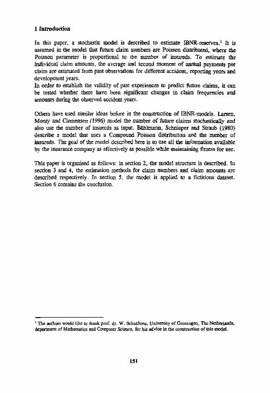
1 Introduction

In this paper, a stochastic model is described to estimate IBNR-reserves. It is assumed in the model that future claim numbers are Poisson distributed, where the Poisson parameter is proportional to the number of insureds. To estimate the individual claim amounts, the average and second moment of annual payments per claim are estimated from past observations for different accident, reporting years and development years. In order to establish the validity of past experiences to predict future claims, it can be tested whether there have been significant changes in claim frequencies and amounts during the observed accident years.

Others have used similar ideas before in the construction of IBNR-models. Larsen, Monty and Clemensen (1996) model the number of future claims stochastically and also use the number of insureds as input. Bühlmann, Schnieper and Straub (1980) describe a model that uses a Compound Poisson distribution and the number of insureds. The goal of the model described here is to use all the information available by the insurance company as effectively as possible while maintaining fitness for use.

This paper is organised as follows: in section 2, the model structure is described. In section 3 and 4, the estimation methods for claim numbers and claim amounts are described respectively. In section 5, the model is applied to a fictitious dataset. Section 6 contains the conclusion.

1 The authors would like to thank prof. dr. W. Schaafsma, University of Groningen, The Netherlands, department of Mathematics and Computer Science, for his advice in the construction of this model.

151

2 General model assumptions

In this section, the mathematical structure of the model is described. The time frame is defined in the first subsection, the stochastic model structure in the second.

2.1 Time frame

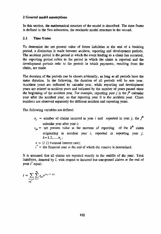
To determine the net present value of future liabilities at the end of a booking period, a distinction is made between accident, reporting and development periods. The accident period is the period in which the event leading to a claim has occurred, the reporting period refers to the period in which the claim is reported and the development periods refer to the periods in which payments, resulting from the claim. are made.

The duration of the periods can be chosen arbitrarily, as long as all periods have the same duration. In the following, the duration of all periods will be one year. Accident years are indicated by calendar year, while reporting and development years are related to accident years and indicated by the number of years passed since the beginning of the accident year. For example, reporting year j is the jth calendar year after the accident year, so that reporting year 0 is the accident year. Claim numbers are observed separately for different accident and reporting years.

The following variables are defined:

nij = number of claims incurred in year i and reported in year j, the jth calendar year after year i;

Sijk = net present value at the moment of reporting of the kth claim

originating in accident year i, reported in reporting year j, k=l2 ,,...,nij;

v = 1/ (1 -l-annual interest rate); i* = the financial year at the end of which the reserve is determined.

It is assumed that all claims are reported exactly in the middle of the year. Total liabilities, denoted by 1, with respect to incurred but unreported claims at the end of year i* equal:

152

2.2 Description of the stochastic model

For the determination of the IBNR-reserve at the end of year i*, a stochastic variable Nij is defined with outcome nij. It is assumed, that Nij is Poisson distributed with

parameter and that is proportional to the number of insureds xi in accident

year i and an expected claim frequency , depending on the accident year and the

reporting year. The claim frequency with outcome is defined as:

The assumption of Poisson distributed claim numbers is made because the Poisson distribution is an adequate distribution to model stochastic events occurring with a small probability.

Furthermore, stochastic variables Sijk with outcomes sijk are defined. Lij represents

the net present value of all future liabilities to be taken-into account at the end of year i* resulting from claims incurred in year i, with , and reported in reporting year j. For the IBNR-reserve, only claims that have incurred in year i, with , and will be reported in year j, with , have to be taken into account. is

defined as:

The net present value at the end of year i* of the total of future liabilities is defined by L and equals:

It is assumed that all the Sijk and Nij are mutually independent. Mean and variance

of equal:

Mean and variance of L equal:

153

so that and

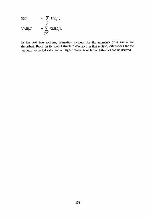
In the next two sections, estimation methods for the moments of N and S are described. Based on the model structure described in this section, estimations for the variance, expected value and all higher moments of future liabilities can be derived.

154

3 Estimation of claim frequencies and the expected number of claims

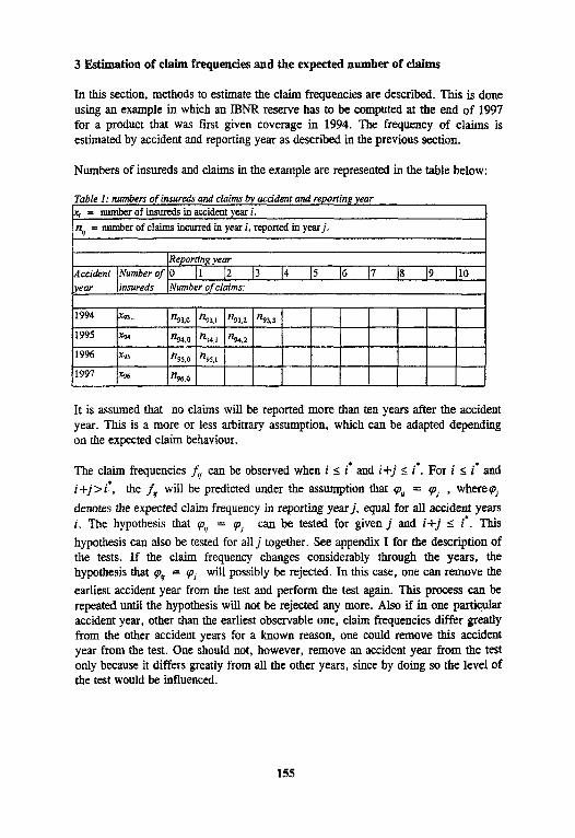
In this section, methods to estimate the claim frequencies are described. ‘This is done using an example in which an IBNR reserve has to be computed at the end of 1997 for a product that was first given coverage in 1994. The frequency of claims is estimated by accident and reporting year as described in the previous section.

Numbers of insureds and claims in the example are represented in the table below:

Table 1: numbers of insureds and claim by accident and reporting year xi = number of insureds in accident year i.

nij = number of claims incurred in year i, reported in year j.

Reporting year Accident Number of 0 1 2 3 4 5 6 7 8 9 10 year insureds Number of claims:

1994 x93 n93,0 n93.1 n93.2 n93.3

1995 x94 n94.0 n94.1 n94.2

1996 x96 n95.0 n95.1

1997 x96 n96.0

It is assumed that no claims will be reported more than ten years after the accident year. This is a more or less arbitrary assumption, which can be adapted depending on the expected claim behaviour.

The claim frequencies fij can be observed when and it For and

the fij will be predicted under the assumption that where

denotes the expected claim frequency in reporting year j, equal for all accident years i. The hypothesis that can be tested for given j and This

hypothesis can also be tested for all j together. See appendix I for the description of the tests. If the claim frequency changes considerably through the years, the hypothesis that will possibly be rejected. In this case, one can remove the

earliest accident year from the test and perform the test again. This process can be repeated until the hypothesis will not be rejected any more. Also if in one particular accident year, other than the earliest observable one, claim frequencies differ greatly from the other accident years for a known reason, one could remove this accident year from the test. One should not, however, remove an accident year from the test only because it differs greatly from all the other years, since by doing so the level of the test would be influenced.

155

Given for all i and given j, the UMVU-estimator of is given by :

See appendix II for a proof.

The expected numbers of claims for future reporting years are predicted by

with and In the example shown in table 1, no

observations are available for Additional assumptions are therefore necessary in this case to estimate These assumptions cannot be tested due to the absence of data. Instead, they will have to be based on more general experience of the actuary regarding late claims.

156

4 Estimation of the distribution of liabilities per claim

In the first subsection of this section, the estimation of the individual claim amounts is discussed. In the second subsection, some comments are made with respect to testing the equality of claim distributions for different accident years.

4.1 Estimation of claim amounts

To estimate the net present value of the liabilities resulting from an individual claim, registrations of benefits paid and additional costs are available. Based on those registrations, expected value, variance and possibly higher moments of the total costs per claim can be estimated. The problem arises that at the instant the reserve has to be determined, many claims have not been fully settled yet. Therefore, annual payments per claim are estimated separately as a function of accident, reporting and development year. The claim amount is estimated as the sum of the estimated payments in different development years.

Bijkl is defined as the total of payments in the lth development year after the accident

year resulting from the kth claim reported in the jth reporting year, incurred in accident year i. In order to take inflation into account, payments done in the past can be adjusted to the level at the end of year i’. Future inflation can be taken into account by assuming an inflation rate for the future and adjusting all payments Bijkl

for which accordingly. Note that in case no payments are made in development year 1, Bijkl equals zero, so that Bijkl is defined for all

All payments are assumed to be made exactly in the middle of the year, so that the delay between reporting and payment is exactly l-j years. Therefore,

The first and second moment of the Sijk can be written in terms of the Bijkl as:

and

157

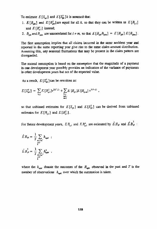
To estimate E [Sijk] and E it is assumed that:

1. E [Bijkl] and E are equal for all k, so that they can be written as E [Bijl]

and E instead;

2. Bijkl and Bijklm are uncorrelated for 1 # m, so that E

The fast assumption implies that all claims incurred in the same accident year and reported in the same reporting year give rise to the same claim amount distribution. Assuming this, any seasonal fluctuations that may be present in the claim pattern are disregarded.

The second assumption is based on the assumption that the magnitude of a payment in one development year possibly provides an indication of the variance of payments in other development years but not of the expected value.

As a result, can be rewritten as:

so that unbiased estimates for E [Sijk] and E can be derived from unbiased

estimates for E [Bijl] and E

For future development years, and are estimated by and :

where the bmjkl denote the outcomes of the Bmjkl observed in the past and T is the

number of observations bmjkl over which the summation is taken.

158

4.2 Testing equality of annual payments for different accident years

It would be interesting to test the hypothesis that annual expected payments or claim amounts after correction for inflation are equal for all observed accident years. For given j and 1, a test statistic can be derived for certain distribution functions of the annual payments. It will not be possible, however, to derive a test for all j and 1 simultaneously at any given level without making assumptions about the dependence structure of the Therefore, testing of the equality of moments of the claim amounts and annual payments is left for further research.

159

5. Calculation of the IBNR-reserve for an existing portfolio

insureds

4,070 239 4,280 223

202 1993 207

1994 4,020 206

1995 4,010 212 1996 4,250 252 1997 4,880 263

In this section, the theory described in the previous sections is applied to an example with fictitious data. In the first subsection, claim frequencies are estimated. In the second subsection, the individual claim amounts are estimated and in the third subsection, the effect of changes in the claim frequencies is investigated.

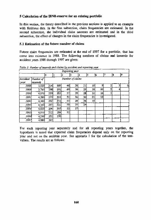
5.1 Estimation of the future number of claims

Future claim frequencies are estimated at the end of 1997 for a portfolio, that has come into existence in 1988. The following numbers of claims and insureds for accident years 1988 through 1997 are given:

Table 2: Number of insureds and claims by accident and reporting year Reporting year

0 1 2 3 4 5 6 7 8 9 Accident [Number of] Number of claims year

1988 3,520 214 189 46 28 21 10 9 2 3 0

1989 3,740 198 191 49 38 29 18 10 5 4 1990 183 57 39 28 16 16 3 1991 201 51 36 30 21 12 1992 4,160 232 55 28 38 19

4,340 221 59 39 29 205 53 37 184 52

190

For each reporting year separately and for all reporting years together, the hypothesis is tested that expected claim frequencies depend only on the reporting year and not on the accident year. See appendix I for the calculation of the test- values. The results are as follows:

160

Table 3 : test values and critical values by reporting year and for all reporting years together Reporting year 0 1 2 3 4 5 6 7 8 total

Test value 13.40 10.36 0.80 3.56 3.27 2.55 1.59 1.37 0.09 37.02

Critical value 2 for

a=10% 14.68 13.36 12.02 10.64 9.24 7.78 6.25 4.61 2.71 57.5

a=5% 16.92 15.50 14.06 12.59 11.07 9.49 7.81 5.99 3.84 61.7

a=1% 21.67 20.09 18.48 16.81 15.09 13.28 11.34 9.21 6.63 70.0

The hypothesis is not rejected for any reporting year nor for all reporting years together (total) at any reasonable test level. It can be discussed whether reporting year 0, the accident year, should be involved in the test, since the IBNR-reserve at the end of any financial year will not provide for claims reported during the accident year. On the other hand, it is logical to assume that claim numbers in different reporting years resulting from the same accident year are always interrelated. Therefore, reporting year 0 is also involved in the test and the test results are shown in the ‘total’-column.

The predictions of the claim frequencies in reporting years 1 through 8 are calculated as the sum of claims in the reporting year divided by the number of insureds in the corresponding accident years. In reporting year 9 and 10, respectively 2/3 and l/3 of the predicted claim frequency in reporting year 8 are taken as prediction values.

The following predictions for claim frequencies are found:

Table 4: predicated claim frequency by Reporting Year Claim frequency

0 0.0537 1 0.0494 2 0.0131 3 0.00871 4 00726 5 030425 6 0.00301 7 0.000883 8 0.000964 9 0.000643

10 0..000321

reporting year

Table 2 can now be extended with expected numbers of future claims:

2 The critical values are based on x2-distributions with df equal to 9 minus the reporting year. For the ‘total’ column, df equals 45. the sum of the df for the separate reporting years.

161

162

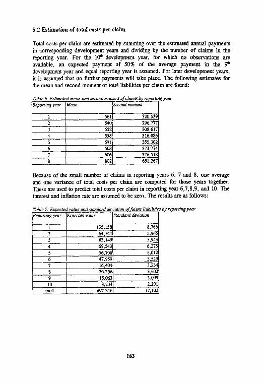
5.2 Estimation of total costs per claim

Total costs per claim are estimated by summing over the estimated annual payments in corresponding development years and dividing by the number of claims in the reporting year. For the 10th development year, for which no observations are available, an expected payment of 50% of the average payment in the 9th development year and equal reporting year is assumed. For later development years, it is assumed that no further payments will take place. The following estimates for the mean and second moment of tots! liabilities per claim are found:

Table 6: Estimated means and second moment of claims by reporting year Reporting year Mean Second moment

1 561 320,539 2 540 296,777 3 552 308,617 4 558 316,086 5 591 355,302 6 608 373,774 7 606 376,518 8 802 651,267

Because of the small number of claims in reporting years 6, 7 and 8, one average and one variance of total costs per claim are computed for those years together. These are used to predict total costs per claim in reporting year 6,7,8,9, and 10. The interest and inflation rate are assumed to be zero. The results are as follows:

1 135,158 8,786 2 64,744 5,965 3 63,149 5,943 4 69,543 6,275 5 56,706 6,012 6 47,959 5,529 7 16,404 3,234 8 20,356 3,602 9 15,063 3,099 10 8,234 2,291

total 497,316 17,102

Table 7: Expected value and standard deviation of future liabilities by reporting year Reporting year Expected value Standard deviation

163

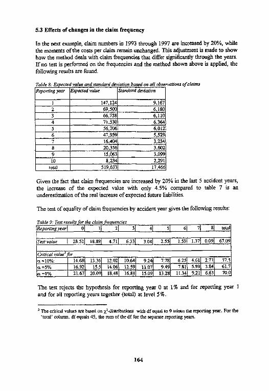
5.3 Effects of changes in the claim frequency

In the next example, claim numbers in 1993 through 1997 are increased by 20%, while the moments of the costs per claim remain unchanged. This adjustment is made to show how the method deals with claim frequencies that differ significantly through the years. If no test is performed on the frequencies and the method shown above is applied, the following results are found.

Table 8: Expected value and standard deviation based on all observations of claims Reporting year Expected value Standard deviation

1 147,124 9,167 2 69,500 6,180

3 66,758 6,110

4 71,530 6,364 5 56,706 6,012

6 47,959 5,529 7 16,404 3,234 8 20,356 3,602

9 15,063 3,099

10 8,234 2,291

total 519.633 17,466

Given the fact that claim frequencies are increased by 20% in the last 5 accident years, the increase of the expected value with only 4.5% compared to table 7 is an underestimation of the real increase of expected future liabilities.

The test of equality of claim frequencies by accident year gives the following results.:

Table 9: Test results for the claim frequencies Reporting year 0 1 2 3 4 5 6 7 8 total

Test value 28.52 18.89 4.71 6.33 3.04 2.55 1.59 1.37 0.09 67.09

Critical value3 for a = 10%: 14.68 13.36 12.02 10.64 9.241 7.78 6.25 4.61 2.71 57.5 a =5% 16.92 15.5 14.06 12.59 11.07 9.49 7.81 5.99 3.84 61.7 a =1% 21.67 20.09 18.48 16.81 15.09 13.28 11.34 9.21 6.63 70.0

The test rejects the hypothesis for reporting year 0 at 1% and for reporting year 1 and for all reporting years together (total) at level 5%.

3 The critical values are based on x2-distributions with df equal to 9 minus the reporting year. For the 'total column, df equals 45, the sum of the df for the separate reporting years.

164

The earliest accident years will now be removed from the test one by one until the hypothesis of equal expected claim frequencies in the remaining accident years is not rejected any more at level 5%. This yields the following results:

165

166

The test for all reporting years together does not reject once all accident years prior to 1993 have been removed. Therefore, the IBNR-reserve is computed with different claim frequencies for 1988 through 1992 and 1993 through 1997 For the total costs per claim, estimates based on the entire period from 1988 through 1997 are used.

9,092 2,407 total 580,467 18,473

The results for accident years 1993 through 1997 cannot be given without additional assumptions. Since the claim frequencies in the first five accident years differ significantly from those in the last five years, there are no unbiased estimators available for the latter. The additional assumptions that will have to be made cannot be tested due to a lack of observations. They will have to be based on more general assumptions about late claims.

One such assumption is that all the claim frequencies with respect to accident years 1993 through 1997 will increase by a constant factor compared to accident years 1988 through 1992. This factor can be estimated by comparing average claim frequencies in 1988 through 1992 with those in 1993 through 1997. In the following, it is assumed that claim numbers in the last five accident years will respectively be 20% and 50% higher than in the first five accident years. The results for this approach are given in the two tables below.

Table 11: Expected value and standard deviation of total future liabilities with 20% higher claim numbers for the last five accident years Reporting year Expected value Standard deviation

1 158,018 9,500 2 77,732 6,536 3 78,056 6,607 4 75,059 6,519 5 68,047 6,586 6 55,996 5,974 7 18,760 3,458 8 22,929 3,823 9 16,779 3,270

10

167

Table 12: Expected value and standard deviation of total future liabilities with 50% higher claim numbers for the last five accident years Reporting year Expected value Standard deviation

1 158,018 9,500 2 77,732 6,536 3 78,056 6,607 4 75,059 6,519 5 85,059 7,363 6 68,051 6,586 7 22,293 3,770 8 26.790 4,132 9 19,352 3,512 10 10,378 2,572

total 620,789 19,156

As one can see, the rejection of the hypothesis of equal claim frequencies for all accident years leads to a considerably higher reserve. By the choice of test level, the actuary’s belief in the hypothesis has a direct effect on the reserve that will be determined.

168

6 Conclusion

This model provides an estimation of expected value, variance and possibly higher moments of the total of future liabilities resulting from incurred but not yet reported claims. By way of statistical testing of additional assumptions, in particular shifts in claim frequencies, the model provides extra insight into the nature of risks undertaken. Statistical testing of the assumptions made leads to a prediction that is more directly related to the company’s claim experience.

In the last section, it is shown that an increase of claim frequencies several yesrs after the earliest observable accident year may lead to a serious underestimation of future liabilities in case all past accident years are used to determine the IBNR- reserve. By testing the equality of claim frequencies, this underestimation can be detected. To correct it, however, no explicit procedure can he prescribed.

The test results do not provide strict guidelines to determine an IBNR-reserve, but can only be seen as a way of providing extra insight to the nature of risks. The interpretation of the test results and the way estimations of future payments are made in the absence of past observations is still largely dependent on specific choices to be made by the actuary.

169

References

Bühlmann, Schnieper, Straub (1980). Claims Reserves in Casualty Insurance based on a Probabilistic Model; Mitteilungen der Vereinigung schweizerischer Versicherungsmathematiker p-21-46.

Dudewicz, Mishra (1988). Modern Mathematical Statistics, Wiley & Sons.

Van Eeghen (1981). Loss Reserving Methods.

Larsen, Monty, Clemmensen (1996). Dynamic loss reserving in a collective model. XXVII ASTIN Colloquium Kopenhagen p.403.

Mack (1994). Which Stochastic Model is Underlying the Chain Ladder Method? IME 15 (1994), 133-138.

Mack (1996). Stochastic Analysis of the Chain Ladder Method. Handout at ASTIN Meeting Amsterdam December 1996.

Mood, Graybill, Boes (1974). introduction to the Theory of Statistics, McGraw Hill International.

170

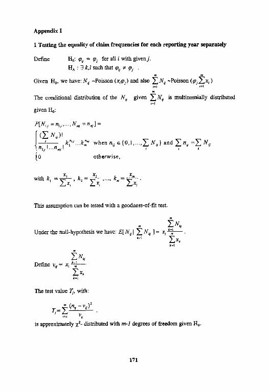
Appendix I

1 Testing the equality of claim frequencies for each reporting year separately

Define for all i with given j.

such that

Given , we have: ~Poisson and also ~Poisson i=l i=l

The conditional distribution of the Nij given is multinomially distributed i=l

given Ho:

when and

0 otherwise,

with

This assumption can be tested with a goodness-of-fit test.

Under the null-hypothesis we have:

Define

The test value Tj, with:

is approximately x2- distributed with m-l degrees of freedom given Ho.

171

2 Testing the equality of expected claim frequencies for ail reporting years together

Null hypothesis and alternative are now as follows:

Ho: for all j we have: for all i with given j.

for which 3 k, l for which

If Ho holds, then all Tj are x2- distributed. Also the sum of the Tj is then x2- distributed. The number of degrees of freedom of the sum, which is used as test value, now equals the sum of the degrees of freedom of the separate Tj.

172

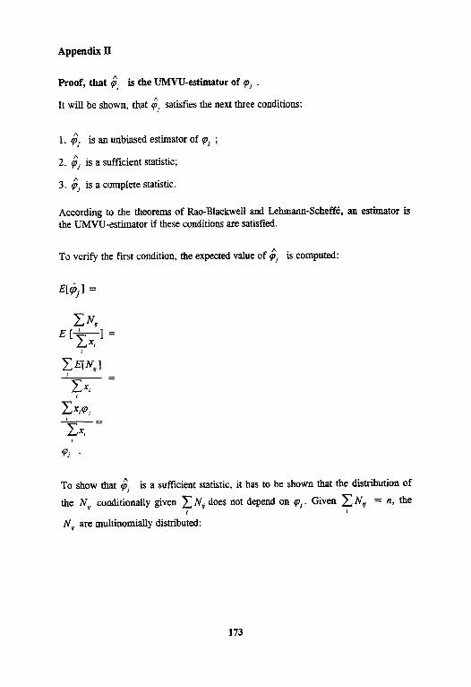
Appendix II

Proof, that is the UMVU-estimator of .

It will be shown, that satisfies the next three conditions:

1. is an unbiased estimator of ;

2. is a sufficient statistic;

3. is a complete statistic.

According to the theorems of Rao-Blackwell and Lehmann-Scheffé, an estimator is the UMVU-estimator if these conditions are satisfied.

To verify the first condition, the expected value of is computed:

To show that , is a sufficient statistic, it has to be shown that the distribution of

the Nÿ conditionally given does not depend on . Given the

Nÿ are multinomially distributed:

173

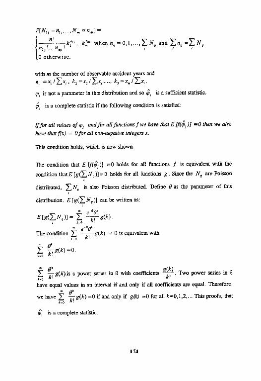
when and

with m the number of observable accident years and

is not a parameter in this distribution and so is a sufficient statistic.

is a complete statistic if the following condition is satisfied:

If for all values of and for all functions f we have that then we also

have that f(x) = 0 for all non-negative integers x.

This condition holds, which is now shown.

The condition that holds for all functions f is equivalent with the

condition that holds for all functions g. Since the Nÿ are Poisson

distributed, is also Poisson distributed. Define as the parameter of this

distribution can be written as:

The condition is equivalent with

is a power series in with coefficients . Two power series in

have equal values in an interval if and only if all coefficients are equal. Therefore,

we have if and only if g(k) =0 for all k=0,1,2,... This proofs, that

is a complete statistic.

174