U.S. Department of the InteriorU.S. Geological Survey

Open-File Report 2015-1126

Prepared in cooperation with the U.S. Fish and Wildlife Service

A Stochastic Population Model to Evaluate Moapa Dace (Moapa coriacea) Population Growth Under Alternative Management Scenarios

U.S. Department of the Interior U.S. Geological Survey

A Stochastic Population Model to Evaluate Moapa Dace (Moapa coriacea) Population Growth Under Alternative Management Scenarios

By Russell W. Perry, Edward C. Jones, and G. Gary Scoppettone

Prepared in cooperation with the U.S. Fish and Wildlife Service

Open-File Report 2015-1126

U.S. Department of the Interior SALLY JEWELL, Secretary

U.S. Geological Survey Suzette M. Kimball, Acting Director

U.S. Geological Survey, Reston, Virginia: 2015

For more information on the USGS—the Federal source for science about the Earth, its natural and living resources, natural hazards, and the environment—visit http://www.usgs.gov/ or call 1–888–ASK–USGS (1–888–275–8747).

For an overview of USGS information products, including maps, imagery, and publications, visit http://www.usgs.gov/pubprod/.

Any use of trade, firm, or product names is for descriptive purposes only and does not imply endorsement by the U.S. Government.

Although this information product, for the most part, is in the public domain, it also may contain copyrighted materials as noted in the text. Permission to reproduce copyrighted items must be secured from the copyright owner.

Suggested citation: Perry, R.W., Jones, E.C., and Scoppettone, G.G., 2015, A stochastic population model to evaluate Moapa dace (Moapa coriacea) population growth under alternative management scenarios: U.S. Geological Survey Open-File Report 2015-1126, 46 p., http://dx.doi.org/10.3133/ofr20151126.

ISSN 2331-1258 (online)

iii

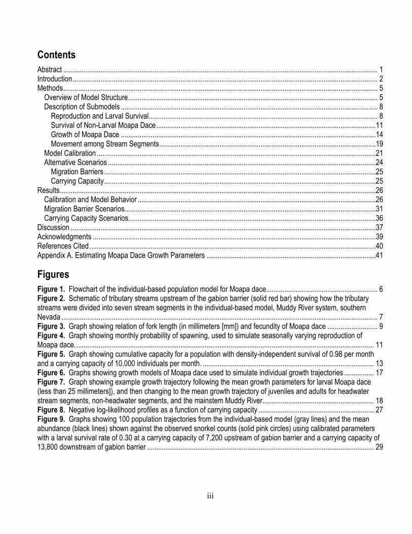
Contents Abstract ......................................................................................................................................................................... 1 Introduction .................................................................................................................................................................... 2 Methods ......................................................................................................................................................................... 5

Overview of Model Structure ...................................................................................................................................... 5 Description of Submodels .......................................................................................................................................... 8

Reproduction and Larval Survival ........................................................................................................................... 8 Survival of Non-Larval Moapa Dace ......................................................................................................................11 Growth of Moapa Dace .........................................................................................................................................14 Movement among Stream Segments ....................................................................................................................19

Model Calibration ......................................................................................................................................................21 Alternative Scenarios ................................................................................................................................................24

Migration Barriers ..................................................................................................................................................25 Carrying Capacity ..................................................................................................................................................25

Results ..........................................................................................................................................................................26 Calibration and Model Behavior ................................................................................................................................26 Migration Barrier Scenarios .......................................................................................................................................31 Carrying Capacity Scenarios .....................................................................................................................................36

Discussion ....................................................................................................................................................................37 Acknowledgments ........................................................................................................................................................39 References Cited ..........................................................................................................................................................40 Appendix A. Estimating Moapa Dace Growth Parameters ...........................................................................................41

Figures Figure 1. Flowchart of the individual-based population model for Moapa dace............................................................ 6 Figure 2. Schematic of tributary streams upstream of the gabion barrier (solid red bar) showing how the tributary streams were divided into seven stream segments in the individual-based model, Muddy River system, southern Nevada .......................................................................................................................................................................... 7 Figure 3. Graph showing relation of fork length (in millimeters [mm]) and fecundity of Moapa dace ........................... 9 Figure 4. Graph showing monthly probability of spawning, used to simulate seasonally varying reproduction of Moapa dace. ................................................................................................................................................................ 11 Figure 5. Graph showing cumulative capacity for a population with density-independent survival of 0.98 per month and a carrying capacity of 10,000 individuals per month. ............................................................................................ 13 Figure 6. Graphs showing growth models of Moapa dace used to simulate individual growth trajectories ................ 17 Figure 7. Graph showing example growth trajectory following the mean growth parameters for larval Moapa dace (less than 25 millimeters]), and then changing to the mean growth trajectory of juveniles and adults for headwater stream segments, non-headwater segments, and the mainstem Muddy River. ........................................................... 18 Figure 8. Negative log-likelihood profiles as a function of carrying capacity .............................................................. 27 Figure 9. Graphs showing 100 population trajectories from the individual-based model (gray lines) and the mean abundance (black lines) shown against the observed snorkel counts (solid pink circles) using calibrated parameters with a larval survival rate of 0.30 at a carrying capacity of 7,200 upstream of gabion barrier and a carrying capacity of 13,800 downstream of gabion barrier .......................................................................................................................... 29

iv

Figure 10. Graph showing 100 population trajectories from the individual-based model (gray lines) and mean abundance (black line) shown against the observed snorkel counts (solid pink circles) using calibrated parameters with a larval survival rate of 0.30 at a carrying capacity of 7,200 upstream of gabion barrier and a carrying capacity of 13,800 downstream of gabion barrier. ......................................................................................................................... 30 Figure 11. Time-series of mean monthly population abundance showing differences in the equilibrium population size among four alternative scenarios of migration barriers ....................................................................... 31 Figure 12. Boxplots showing differences among the distribution of simulated population abundance at the end of the 50-year time horizon for the four alternative scenarios of migration barriers at three initial population sizes (N0=10, 50, and 500) ........................................................................................................................ 32 Figure 13. Time series of the mean monthly abundance for population realizations with 0, 1, and 2 local extinctions, simulated under the baseline scenario when Pedersen weirs and the gabion barrier were in place, starting with an initial population size of 10 fish ........................................................................................................... 33 Figure 14. Probability of a local extinction as a function of initial population size....................................................... 34 Figure 15. Boxplots showing distribution of population sizes at the end of 50-year simulations under the baseline scenario for 100 runs of the individual-based model. ................................................................................................... 36

Tables Table 1. Proportion of total carrying capacity upstream of the gabion barrier assigned to each stream segment. ..... 14 Table 2. Life stage and segment-specific growth parameters used to simulate individual growth trajectories of Moapa dace. ............................................................................................................................................................ 16 Table 3. Mean proportion of the population in each life stage in December of the last time step for four alternative scenarios of migration barriers. .................................................................................................................. 35 Table 4. Mean population abundance in each life stage in December of the last time step for four alternative scenarios of migration barriers. ................................................................................................................................... 35

Conversion Factors International System of Units to Inch/Pound

Multiply By To obtain

Length millimeter (mm) 0.03937 inch (in.)

kilometer (km) 0.6214 mile (mi)

Temperature in degrees Celsius (°C) may be converted to degrees Fahrenheit (°F) as follows:

°F=(1.8×°C)+32

1

A Stochastic Population Model to Evaluate Moapa Dace (Moapa coriacea) Population Growth Under Alternative Management Scenarios

By Russell W. Perry, Edward C. Jones, and G. Gary Scoppettone

Abstract The primary goal of this research project was to evaluate the response of Moapa dace (Moapa

coriacea) to the potential effects of changes in the amount of available habitat due to human influences such as ground water pumping, barriers to movement, and extirpation of Moapa dace from the mainstem Muddy River. To understand how these factors affect Moapa dace populations and to provide a tool to guide recovery actions, we developed a stochastic model to simulate Moapa dace population dynamics. Specifically, we developed an individual based model (IBM) to incorporate the critical components that drive Moapa dace population dynamics. Our model is composed of several interlinked submodels that describe changes in Moapa dace habitat as translated into carrying capacity, the influence of carrying capacity on demographic rates of dace, and the consequent effect on equilibrium population sizes. The model is spatially explicit and represents the stream network as eight discrete stream segments. The model operates at a monthly time step to incorporate seasonally varying reproduction. Growth rates of individuals vary among stream segments, with growth rates increasing along a headwater to mainstem gradient. Movement and survival of individuals are driven by density-dependent relationships that are influenced by the carrying capacity of each stream segment.

First, we calibrated the model to a historical time series of Moapa dace abundance estimates. The goal of the calibration was to estimate unknown parameters such as larval survival, carrying capacity of the tributary streams harboring the population of Moapa dace upstream of the gabion barrier, and carrying capacity of the mainstem Muddy River and tributaries. Based on historical abundance estimates, we found that the carrying capacity of the mainstem Muddy River was nearly twice the capacity of the tributary streams where Moapa dace have resided for the past 20 years.

Given the calibrated model, we then conducted simulations to assess (1) the effect of altering migration barriers that restrict upstream and downstream movement of dace, and (2) the effect of changes in carrying capacity on equilibrium population sizes. We found that barriers to upstream movement led to extinction of subpopulations upstream of the barriers when initial population sizes were small. The probability of one or more subpopulations going extinct over a 50-year time horizon was >0.80 at initial population sizes of 10 non-larval and 70 larval dace, and was >0.40 at initial population sizes of 50 non-larval and 350 larval dace. The probability of a subpopulation going extinct decreased to zero when the initial population size exceeded 100 non-larval dace. Removal of upstream migration barriers eliminated extinctions of subpopulations, even at low initial population sizes. Compensatory mechanisms such as density-dependent survival and movement acted to buffer against local extinctions because stream segments could be quickly repopulated by dispersal when fish could access all stream segments.

2

Providing access to the mainstem Muddy River through removal of a gabion barrier that restricted upstream and downstream movement increased total population size from about 875 to 3,000 individuals. Additionally, because of higher growth rates of individuals in the mainstem Muddy River, the size structure of the population shifted towards larger individuals with higher fecundity, thereby increasing reproductive capacity of the population.

Increasing or decreasing the total carrying capacity of all stream segments resulted in changes in equilibrium population size that were directly proportional to the change in capacity. However, changes in carrying capacity to some stream segments but not others could result in disproportionate changes in equilibrium population sizes by altering density-dependent movement and survival in the stream network. These simulations show how our IBM can provide a useful management tool for understanding the effect of restoration actions or reintroductions on carrying capacity, and, in turn, how these changes affect Moapa dace abundance. Such tools are critical for devising management strategies to achieve recovery goals.

Introduction The Moapa dace (Moapa coriacea) is a thermophilic minnow native to the Muddy River system

near Las Vegas, in southern Nevada. The range of Moapa dace is constrained to areas with water temperatures between 26.0 and 32.0 °C, which restrict them to the upper 2 km of the Muddy River and several small tributaries fed by warm springs. The general area where they occur is known as the Warm Springs Area. The Moapa dace was recognized as endangered in 1967 (Udall, 1967) and federally listed as such in 1973 due to its restricted range and population decline from historical levels (U.S. Department of the Interior, 1973). In 1995, exotic blue tilapia (Oreochromis aureus) invaded Warm Springs, and Moapa dace abundance declined shortly thereafter. Installation of a gabion barrier on the lower Plummer Stream (referred to as “Refuge Stream” in the associated Recovery Plan; U.S. Fish and Wildlife Service, 1996.) allowed blue tilapia to be eradicated upstream of this barrier. In 2014, these headwater streams harbored the remaining population of Moapa dace. Before introduction of blue tilapia, the Moapa dace population ranged from 3,000 to 5,000 fish, but since their habitat has been restricted to headwater streams upstream of the gabion barrier, their observed population has ranged from 439 to 1,727 individuals based on biannual snorkel counts through August 2013. Life history, abundance, and distribution information on Moapa dace are available in Scoppettone and others (1992) and Scoppettone (1993).

As a result of geothermal heating, water enters the Warm Springs pools at about 32 °C and cools as it flows downstream. Although water temperatures and flow rates in the Warm Springs Area show little seasonal variation, these stable environmental conditions may change because of human influences. Water removals from the Muddy River aquifer have been shown to reduce the volume of water entering the spring system, which will reduce the volume of water flowing into the headwater streams (Mayer and Congdon, 2008). Reduced spring flow has been shown to reduce the amount of suitable habitat available for the Moapa dace (Hatten and others, 2013). However, the effect of reduced spring flow on the thermal environment and the consequent effect on habitat suitability for Moapa dace is less certain. Changes in the amount of habitat available for Moapa dace owing to factors such as blue tilapia invasion or reduced spring flows will alter the carrying capacity of the environment to support Moapa dace. Declines in carrying capacity, in turn, may hamper efforts to restore or even maintain Moapa dace populations. Understanding how changes in carrying capacity influence population dynamics of Moapa dace is critical for devising strategies to meet recovery goals.

3

The primary goal of our project is to evaluate the response of the Moapa dace population to the potential effects of human influences such as ground water pumping, movement barriers, and reintroduction of Moapa dace to the mainstem Muddy River. To understand how these factors affect Moapa dace populations and to provide a tool to guide recovery actions, we developed a stochastic model to simulate Moapa dace population dynamics. Specifically, we developed an individual based model (IBM) to incorporate the critical components that drive Moapa dace population dynamics. Our model is composed of several interlinked submodels that describe changes in Moapa dace habitat as translated into carrying capacity, the influence of carrying capacity on demographic rates of dace, and the consequent effect on equilibrium population sizes.

Numerous important physiological, ecological, and behavioral characteristics of Moapa dace suggest that size structure is a critical component to include in a population dynamics model for dace. First, fecundity of Moapa dace increases with size, and thus larger individuals will contribute more recruits to the population than small individuals (Scoppettone and others, 1992). With size-dependent fecundity, the size structure of the population can be an important determinant of population growth rate. Prior to invasion of blue tilapia, Moapa dace up to 120 mm fork length (FL) commonly were observed in the mainstem Moapa River, but a FL of just 70 mm is near the upper end of the size distribution since their restriction to smaller headwater streams (Hereford, 2014b). Absence of highly fecund, large individuals, therefore, may affect how quickly the population recovers from population declines. Second, survival likely differs among life stages, particularly for larval (<25 mm FL) and non-larval dace (≥25 mm FL). For example, Scoppettone and Burge (1994) estimated survival of 32 percent during the first year of life (larvae to 45 mm FL), but observed 60 percent survival over the second year (45–55 mm FL). Therefore, an individual’s growth rate will affect how long it remains within a given life stage, in turn influencing cumulative survival. These findings suggest that a population model for Moapa dace should include size-dependent growth, fecundity, and survival.

Size of Moapa dace also is correlated with temperature and the size of habitat units (depth, water velocity, and discharge), which may influence growth rates. Scoppettone and others (1992) observed that fish size increased with the range of water depth and volume used by Moapa dace. Size of Moapa dace generally appears to increase along a headwater-to-mainstem gradient. Moving along this gradient, water temperature decreases while water volume increases. It is unclear whether size of Moapa dace is organized along this gradient because of ontogenetic shifts in thermal preferenda or because of better ability to maintain feeding stations in higher velocity environments. We hypothesize that both mechanisms likely co-evolved to the tight linkage between water temperature and water volume in this system. For example, a hypothesis explaining the absence of large individuals in the restricted headwater population is that metabolic requirements at high temperatures reduce growth rates of larger individuals, thereby reducing their maximum attainable size (G. Scoppettone, U.S. Geological Survey, oral commun., 2010). These observations suggest that Moapa dace may require a diversity of channel size and water temperature for full expression of all possible size classes, which, in turn, may influence population growth rates owing to size-dependent fecundity. To incorporate these dynamics in our population model, we allow growth rates to vary among different stream segments that are represented in the model.

Movement behavior of Moapa dace, connectivity of the channel network in the Warm Springs Area, and current (2014) absence of dace from the mainstem Muddy River also are important features to include in the population dynamics model. Historically, the dace population appeared to move extensively throughout the channel network of headwater springs and Muddy River. For example, population counts varied little between 1986 and 1988, but the spatial distribution of the population varied considerably among years (Scoppettone and others, 1992). During these surveys, over one-half of

4

the population was observed in the mainstem Muddy River in one year, whereas only 16 percent were found in the mainstem in another year, with the balance of the population present each year in the headwater streams. Spawning is hypothesized to occur only in the higher water temperatures of headwater springs compared to the mainstem (Scoppettone and others, 1992), yet larger, more fecund individuals occupied mainstem channels. These findings indicate that high rates of movement throughout the channel network of the Muddy River system likely are an adaptive strategy that allows dace to capitalize on spatial variation in the environment (water temperature, volume, and velocity) in order to persist under such conditions. Thus, connectivity among channels and use of the mainstem Muddy River may be requisite for the long-term persistence of Moapa dace.

In the past, the channel network of the Warm Springs Area has been highly fragmented, with numerous barriers to upstream and downstream movement. Furthermore, Moapa dace have been extirpated from the mainstem Muddy River since the introduction of blue tilapia (Scoppettone and others, 2005). In 2012, however, movement barriers in headwater stream segments have been removed, and, since the occurrence of a large flood event in September 2014, some passage is allowed through the gabion barrier. When evaluating the population response of Moapa dace, we constructed a model that accounts for the spatial structure of the entire channel network that once was inhabited by the Moapa dace. This approach views the whole population (meta-population) as a collection of subpopulations with movement rates among subpopulations dictated by the spatial structure of the channel network.

Factors affecting the amount of available habitat or the ability of Moapa dace to move among habitats ultimately will influence the carrying capacity of the Warm Springs Area to support Moapa dace. These factors include changes in stream discharge, presence of invasive species, movement barriers, and extirpation from the mainstem Muddy River. Population trajectories over the past 30 years provide evidence that Moapa dace populations may have been constrained by carrying capacity and have responded to increases in carrying capacity. For example, snorkel surveys indicate that the population size in the area upstream of the gabion barrier remained relatively constant for more than 20 years (1985–2008), ranging from about 800 to 1,200 individuals. This long period of relative stability suggests that the population may have been at or near the capacity of the available habitat upstream of the gabion barrier. Although the population declined to only 439 observed individuals in 2008 for unknown reasons, the population has since rebounded to 1,727 fish as of August 2013. This increase is presumably owing to habitat restoration of the Pedersen and Apcar streams that likely increased carrying capacity upstream of the gabion barrier.

Density dependent processes, such as intraspecific competition, are weak controls on population growth rate when abundance is much less than carrying capacity, but act to decrease population growth rate as carrying capacity is approached. Therefore, populations tend to increase when abundance is much less than carrying capacity, but remain at a stable equilibrium when abundance is near carrying capacity. We explicitly incorporated density-dependent processes in our model in two ways. First, we used a density-dependent survival model that decreased survival as carrying capacity was approached, but increased survival when population size was much less than carrying capacity. Second, we used a density-dependent movement model based on ideal free distribution theory (Fretwell and Lucas, 1970), where individuals move to stream segments offering high profitability as measured in terms of survival. To estimate the carrying capacity of Warm Springs Area, we calibrated our IBM of Moapa dace by fitting it to the 30-year time series of snorkel counts. Given estimates of carrying capacity obtained through calibration, we then used the model to evaluate alternative scenarios relating to changes in carrying capacity, movement barriers, and access to the mainstem Muddy River.

5

To evaluate alternative scenarios, we compared equilibrium population sizes, population growth rates, life stage structure (larval, juvenile, and reproductive sized fish), and subpopulation extinction probabilities. Although we evaluated the probability of extinction for different subpopulations, our model predicted a very low probability that the entire population would go extinct because density-dependent mechanisms increased population growth rates at low population size, thereby reducing extinction risk. Although extinction probabilities are an important metric to consider, the minimum observed population abundance of Moapa dace (439 fish) is much greater than the level of abundance at which processes such as demographic stochasticity and allee effects would be expected to affect extinction probabilities. Nonetheless, the Moapa dace population is fragmented by movement barriers, occupies a small fraction of its historical range, and remains much less than recovery goals (6,000 fish; U.S. Fish and Wildlife Service, 1996). Therefore, although extinction of Moapa dace remains a concern, our population model is better suited to understanding how the amount of available habitat affects carrying capacity, and, in turn, population size. Additionally, our model is spatially explicit, incorporating linkages among different stream sections that allow movement barriers to be assessed. These attributes of our model provide fisheries managers with a quantitative tool for understanding how alternative management actions will affect recovery of the Moapa dace population.

Methods Overview of Model Structure

Key characteristics of Moapa dace biology, the nature of the stream network structure, and relevant management questions dictated the type of population model we used to simulate Moapa dace biology. Based on these characteristics, we constructed an individual-based model (IBM). The key characteristics that required use of an IBM included:

• Growth rates vary among locations in the Warm Springs Area. • Fecundity depends on size of individuals, which, in turn, depends on growth rate. • Movement barriers restrict access to some locations. • Survival is driven by carrying capacity of different stream segments. • Survival differs among life stages (larvae, non-larvae), linked to growth rate. • Management scenarios alter movement barriers or change carrying capacity.

An IBM is the ideal framework for incorporating these characteristics because the state of each individual at each time step is tracked throughout its life. In our model, these states include an individual’s size, sex, location, and life stage (fig. 1). Demographic processes such as growth, reproduction, and survival then depend on the state of the individual, and the population structure (spatial distribution, size distribution, and abundance) arises as an emergent property of the collection of individuals (fig. 1).

An IBM is a stochastic model, meaning that the outcome of demographic processes arises probabilistically. This allowed us to incorporate effects such as demographic stochasticity, a process that can increase extinction probability at very low population sizes. Because the model is stochastic, there is a different outcome each time the model is run. This allowed us to examine not only the mean abundance through time, but how abundance varies over multiple model runs (referred to as “realizations” of the model).

6

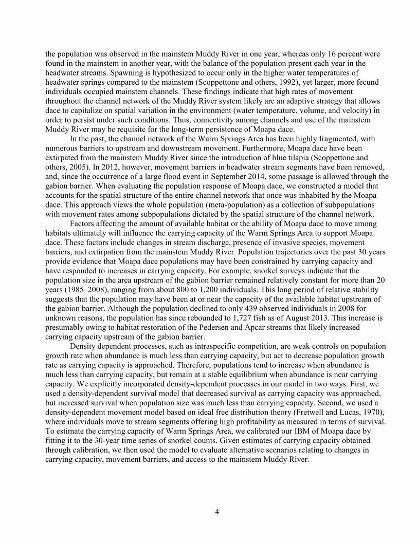
Figure 1. Flowchart of the individual-based population model for Moapa dace. Ovals represent the state of an individual, diamonds indicate a Bernoulli trial or a decision point, solid rectangles are model processes affecting the state of the individual, and dashed rectangles represent factors affecting model processes.

7

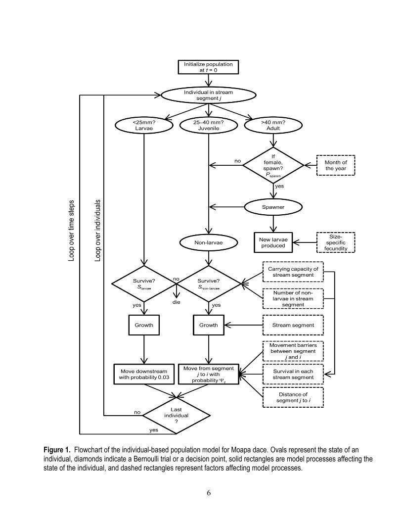
The IBM of Moapa dace is spatially explicit, allowing us to emulate processes such as location-dependent growth rate, movement barriers, and inhabitation of the mainstem Muddy River. We divided the stream network system into eight discrete stream segments based on location of historical movement barriers, confluences of different streams, and distinction between headwater spring segments and non-headwater segments (fig. 2). The seven stream segments upstream of the gabion barrier represent the primary remaining habitat harboring Moapa dace after the invasion by blue tilapia in 1995 until the recent (2014) flood event that damaged the gabion barrier. Segment 8 represents all available habitats downstream of the gabion barrier, which includes the mainstem Muddy River and other tributaries that harbored Moapa dace from 1985 to 1995, the period during which snorkel abundance estimates were available for calibration. Each stream segment had an associated carrying capacity, which was determined by calibrating the model to observed snorkel census data.

To incorporate seasonally varying dynamics, we constructed the model to run at a monthly time step. Thus, all demographic rates (growth, survival, and movement) are monthly rates. The choice of time step was dictated primarily by seasonally varying reproduction. Reproduction occurs year round, but with a clear peak in the spring (Scoppettone and others, 1992). Thus, because spawning was continuous and did not occur at a discrete time of the year, an annual time step could introduce considerable bias in the population dynamics.

Figure 2. Schematic of tributary streams upstream of the gabion barrier (solid red bar) showing how the tributary streams were divided into seven stream segments in the individual-based model, Muddy River system, southern Nevada. Dotted green lines show where segments without movement barriers were divided. The two open bars indicate segments separated by barriers to upstream movement in Pedersen stream.

8

At each time step, individuals reproduce, survive, grow, and then move at the end of the time step (fig. 1). This sequence of events is an important component of the underlying structure of the model. Each event in the sequence is driven by an underlying submodel that determines how each demographic process is applied to fish of a given size and life stage in each stream segment. In the sections that follow, we describe in detail each of these sub-models used to simulate demographic processes, the procedures we used to calibrate the model, and given the calibrated model, the alternative scenarios we assessed to understand the potential response of the Moapa dace population to management actions that alter movement barriers or carrying capacity.

Description of Submodels

Reproduction and Larval Survival Some aspects of Moapa dace reproductive ecology are well-known, but others are poorly

understood. For example, a strong relation between fecundity and fish size has been well established (Scoppettone and others, 1992). Additionally, based on larvae counts during snorkel surveys, reproduction is known to occur year round, with distinct seasonal peaks during the spring (Scoppettone and others, 1992). However, less well known aspects of Moapa dace reproductive ecology include:

1. whether individuals spawn once or numerous times throughout the year; 2. fraction of total fecundity spawned during each spawning even; 3. probability of an egg hatching, given it has been laid; 4. monthly survival probability of larval-sized Moapa dace; and 5. how reproduction varies spatially throughout the Muddy River system.

For example, Scoppettone and others (1992) found that eggs skeins within Moapa dace were in different stages of development, indicating that only some fraction of the total fecundity is laid on a given spawning event, but this fraction remains unknown. Furthermore, larvae have been observed only near headwater tributaries (Scoppettone and others, 1992), but it is unclear whether this pattern results from spawning taking place everywhere with unsuccessful reproduction in lower segments, or whether individuals move upstream and spawn only in headwater segments.

To simulate reproduction of Moapa dace, we used historical information and datasets to parameterize the IBM. For example, our model incorporates size-dependent fecundity and seasonal reproduction. However, uncertainties in the reproductive ecology of Moapa dace required making a number of simplifying assumptions. The primary assumptions are (1) Moapa dace spawn once per year, (2) reproduction occurs everywhere, and (3) larval survival is constant across stream segments.

9

We used an allometric growth model to simulate the number of eggs produced by an individual Moapa dace as a function of length:

eggs,

if individual is female and 40

0 if individual is male or 40

bi i i

ii

aL i LN

i L + ≥=

<

e (1)

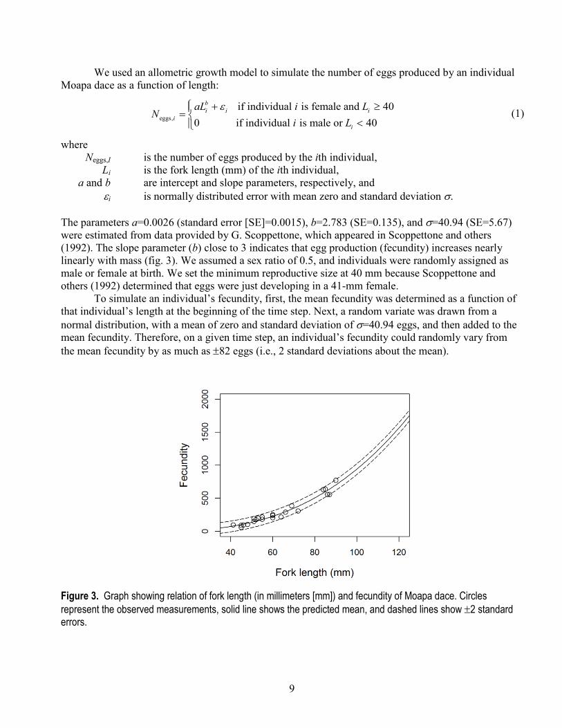
where Neggs,I is the number of eggs produced by the ith individual, Li is the fork length (mm) of the ith individual, a and b are intercept and slope parameters, respectively, and ei is normally distributed error with mean zero and standard deviation σ. The parameters a=0.0026 (standard error [SE]=0.0015), b=2.783 (SE=0.135), and σ=40.94 (SE=5.67) were estimated from data provided by G. Scoppettone, which appeared in Scoppettone and others (1992). The slope parameter (b) close to 3 indicates that egg production (fecundity) increases nearly linearly with mass (fig. 3). We assumed a sex ratio of 0.5, and individuals were randomly assigned as male or female at birth. We set the minimum reproductive size at 40 mm because Scoppettone and others (1992) determined that eggs were just developing in a 41-mm female.

To simulate an individual’s fecundity, first, the mean fecundity was determined as a function of that individual’s length at the beginning of the time step. Next, a random variate was drawn from a normal distribution, with a mean of zero and standard deviation of σ=40.94 eggs, and then added to the mean fecundity. Therefore, on a given time step, an individual’s fecundity could randomly vary from the mean fecundity by as much as ±82 eggs (i.e., 2 standard deviations about the mean).

Figure 3. Graph showing relation of fork length (in millimeters [mm]) and fecundity of Moapa dace. Circles represent the observed measurements, solid line shows the predicted mean, and dashed lines show ±2 standard errors.

10

To simulate seasonally varying spawning, individual fish were randomly assigned a month of spawning at the beginning of each year, with the probability of spawning peaking in the spring. The probability of spawning in a given month was specified by using a truncated normal distribution with a mean spawning date of April 15 and standard deviation of 91.25 days (fig. 4). Females then spawned only if they survived to their randomly drawn month of spawning and only if at least one adult male (≥40 mm FL) was present within the same stream segment.

Given reproduction in a particular month, the number of larvae produced by an individual can be expressed as:

larvae, eggs, laid hatchi iN N p p= (2)

where Nlarvae,i is the number of larvae produced by ith adult spawning female, plaid is the proportion of Neggs,i laid, and phatch is the probability of an egg hatching given it has been laid. We assume that survival of larvae is density independent, and occurs at a constant monthly probability of Slarvae until larvae exceed 25 mm, at which point they become juveniles. At each time step, survival of individual larvae is determined by performing a Bernoulli trial with probability Slarvae. The probability of surviving from an egg to the juvenile stage is:

egg juvenile, laid hatch larvaet

iS p p S→ = (3)

where egg juvenile,iS → is the total survival from the ith egg in a reproductive female until the time at which a

larvae transitions to the juvenile stage t months later. No information exists about the parameters plaid, phatch, and Slarvae. Thus, we fixed plaid and phatch to 1 and estimated Slarvae by calibration (see section, “Model Calibration,” for details). Using this approach, Slarvae in our model represents the monthly survival probability that accounts for the probability that an egg in a reproductive female is laid and hatched, and survives to the juvenile stage.

11

Figure 4. Graph showing monthly probability of spawning, used to simulate seasonally varying reproduction of Moapa dace.

Survival of Non-Larval Moapa Dace Our individual-based model considers three key processes that influence survival: (1)

demographic stochasticity, (2) process error, and (3) density dependence. Demographic stochasticity is the random chance that an individual lives or dies with given probability of survival. Demographic stochasticity is an important mechanism affecting extinction risk when populations are at very low levels. Process error is defined as temporal and spatial variation in the probability of surviving that is caused by fluctuations in the environment. Process error can increase risk of extinction when chance events cause simultaneous decreases in survival over space or when survival remains low over consecutive time periods. Last, competition among individuals for space or food can reduce survival as populations increase and approach the capacity of their environment. At low population levels, density-dependent factors can reduce extinction risk because survival increases in response to reduced competition for resources.

A key challenge in parameterizing a population model is estimating survival rates, particularly for small fish such as Moapa dace. For example, Hereford (2014a) found that bimonthly survival of Moapa dace ranged from about 0.70 to 0.96, and survival varied considerably among stream reaches, seasons, and years.

12

We used a multi-stage stock and recruitment model of Moussalli and Hilborn (1986) based on the Beverton and Holt (1957) model. For Moapa dace, this density-dependent model takes the form

, ,, , 1

, ,

0, , , 1 ,

1i j t

i j ti j t

i j t t i j

NN

NS c

+

→ +

=+

(4)

where , ,i j tN is the number of individuals in life stage i and stream segment j at time t, , , 1i j tN + is the number in stage i and segment j at time t+1, ,i jc is the carrying capacity of life stage i in segment j, 0, , , 1i j t tS → + is the density-independent survival from t to t+1 for life stage i in stream segment j

that is approached as , ,i j tN approaches zero. The parameter 0, , , 1i j t tS → + also is known as the productivity parameter (Moussalli and Hilborn, 1986).

For the Moapa dace IBM, we express this model in terms of survival from one time step to the next:

, , 1, , 1

, ,, ,

0, , , 1 ,

11

i j ti j t t

i j ti j t

i j t t i j

NS

NNS c

+→ +

→ +

= =+

(5)

where , , 1i j t tS → + is the probability of surviving from t to t+1 for life stage i in stream segment j.

For this multistage model of density-dependent survival, carrying capacity has a temporal component such that it represents the number of individuals that can be supported by habitat over one time step of the model (1 month). For this reason, ,i jc may be much higher than the equilibrium population size. Therefore, it is more natural to think of the cumulative capacity, ,i jC , which is the number of individuals that can be supported over some specified number of time steps, n (Moussalli and Hilborn, 1986):

0, , , 1

1,

0, , , 1

1 ,

n

i j t tt

i j ni j t t

t i j

SC

Sc

→ +=

→ +

=

=∏

∑ (6)

For example, for density-independent survival of 0, , , 1i j t tS → + =0.98 per month and carrying capacity of ,i jc=10,000, the cumulative capacity after 1 year is 744 individuals (fig. 5). This example illustrates how carrying capacity as estimated in our analysis will be much higher than the long-term population size at equilibrium. Furthermore, it illustrates how changes in carrying capacity might affect equilibrium population size in nonlinear and disproportionate ways.

13

Figure 5. Graph showing cumulative capacity for a population with density-independent survival of 0.98 per month and a carrying capacity of 10,000 individuals per month.

We modeled survival separately for two life stages, i=larvae, or i=non-larval fish (subadults and

adults). We assumed that survival of larvae was density independent such that ,i jc = ∞ and , , 1i j t tS → + =

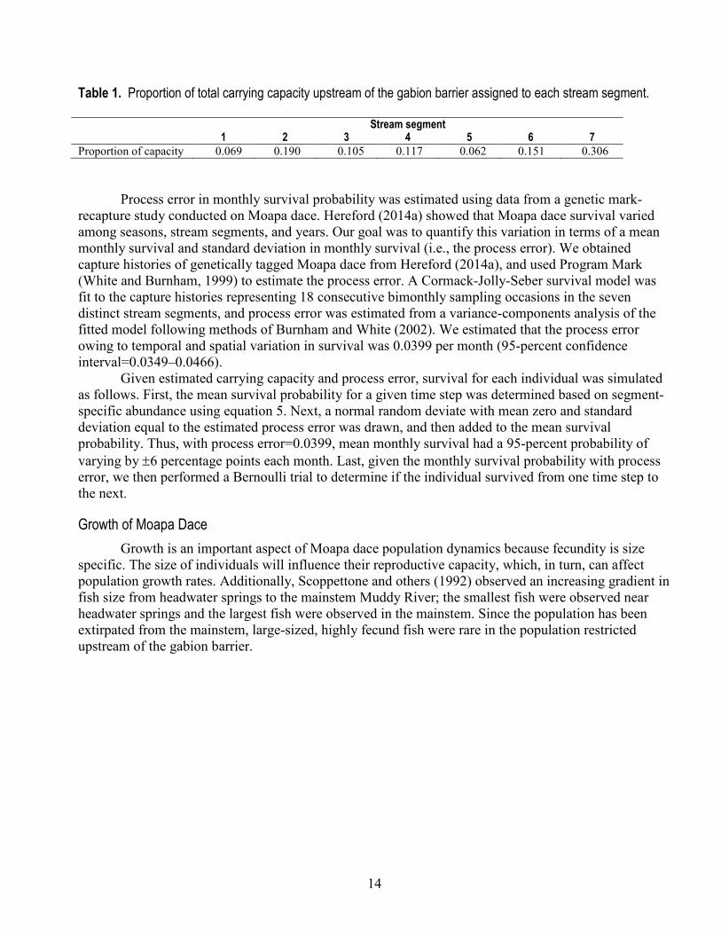
0, , , 1i j t tS → + . Larval survival and other reproductive parameters are unknown, and, therefore, were estimated through calibration (see sections, “Reproduction and Larval Survival” and “Model Calibration,” for details). For non-larval fish, each discrete stream segment in the model was assigned a carrying capacity, which then allowed survival to vary among stream segments depending on segment-specific abundance and capacity. To determine the capacity of each segment, we first used calibration to estimate the carrying capacity of the mainstem Muddy River (stream segment 8) and the total capacity of all stream segments upstream of the gabion barrier (stream segments 1–7). Given an estimate of the total capacity upstream of the gabion barrier, we then used information about relative habitat quality and the length of each stream segment to determine the proportion of the total capacity assigned to each stream segment (table 1). Relative habitat quality was estimated by fitting an N-mixture model (Royle, 2004) to minnow trap catches to relate abundance of Moapa dace in each stream segment to habitat variables such as water depth, velocity, and substrate composition (R.W. Perry, U.S. Geological Survey, unpub. data, 2012). On average, site-specific estimates of habitat quality in stream segment 7 were lower than in other segments, but the greater size of this segment contributed to its overall larger capacity.

14

Table 1. Proportion of total carrying capacity upstream of the gabion barrier assigned to each stream segment.

Stream segment 1 2 3 4 5 6 7

Proportion of capacity 0.069 0.190 0.105 0.117 0.062 0.151 0.306

Process error in monthly survival probability was estimated using data from a genetic mark-recapture study conducted on Moapa dace. Hereford (2014a) showed that Moapa dace survival varied among seasons, stream segments, and years. Our goal was to quantify this variation in terms of a mean monthly survival and standard deviation in monthly survival (i.e., the process error). We obtained capture histories of genetically tagged Moapa dace from Hereford (2014a), and used Program Mark (White and Burnham, 1999) to estimate the process error. A Cormack-Jolly-Seber survival model was fit to the capture histories representing 18 consecutive bimonthly sampling occasions in the seven distinct stream segments, and process error was estimated from a variance-components analysis of the fitted model following methods of Burnham and White (2002). We estimated that the process error owing to temporal and spatial variation in survival was 0.0399 per month (95-percent confidence interval=0.0349–0.0466).

Given estimated carrying capacity and process error, survival for each individual was simulated as follows. First, the mean survival probability for a given time step was determined based on segment-specific abundance using equation 5. Next, a normal random deviate with mean zero and standard deviation equal to the estimated process error was drawn, and then added to the mean survival probability. Thus, with process error=0.0399, mean monthly survival had a 95-percent probability of varying by ±6 percentage points each month. Last, given the monthly survival probability with process error, we then performed a Bernoulli trial to determine if the individual survived from one time step to the next.

Growth of Moapa Dace Growth is an important aspect of Moapa dace population dynamics because fecundity is size

specific. The size of individuals will influence their reproductive capacity, which, in turn, can affect population growth rates. Additionally, Scoppettone and others (1992) observed an increasing gradient in fish size from headwater springs to the mainstem Muddy River; the smallest fish were observed near headwater springs and the largest fish were observed in the mainstem. Since the population has been extirpated from the mainstem, large-sized, highly fecund fish were rare in the population restricted upstream of the gabion barrier.

15

To simulate growth of Moapa dace and to emulate the spatial dynamics, we used a von Bertalanffy growth model (Francis, 1988) that allowed for life stage- and location-specific growth rates. Furthermore, we assumed that individuals grow deterministically but that variation in growth rate arises from variation in growth parameters among individuals. We used a version of the von Bertalanffy growth model that describes growth rate as the change in length from one time step to the next:

1t tL L L+ = + ∆ (7)

( ) ( )1 ktL L L e−

∞∆ = − − (8)

where Lt and Lt+1 is the fork length at time t and t+1, L∆ is the change in fork length (mm) over one time step, L∞ is the asymptotic theoretical maximum fork length (mm), and k is a constant that determines how quickly length approaches L∞. The parameters L∞ and k uniquely determine the growth trajectory, given length at time t (Lt). To drive individual growth trajectories, we assumed that these parameters were drawn from normal distributions for each individual:

( )Normal ,L LL∞ ∞∞ m σ (9)

( )Normal ,k kk m σ (10)

where Lm ∞

and km are the mean L∞ and mean k, respectively, and

Lσ∞

and kσ are the standard deviation of L∞ and k.

We developed four growth models that allowed individuals to grow at different rates, depending on their life stage (larvae or juveniles/adults) and their location in the Muddy River system (headwater springs, non-headwater springs, and the mainstem Muddy River). Where possible, existing data were analyzed to estimate Lm ∞

and km . For larvae, we estimated Lm ∞and km from a study conducted in 1984

(Scoppettone and Burge, 1994), where 140 larval dace were transported to an isolated segment of upper Plummer Spring, and then their fork lengths were measured every 3 months for 3 years (table 2, appendix A). Growth of non-larval fish in this study might have been constrained by warm water temperatures or low dissolved oxygen concentrations in the upper Plummer Spring (Scoppettone and Burge, 1994). Therefore, we also analyzed size data obtained by Hereford (2014b), where juvenile and adult individuals were trapped with minnow traps over a 3-year period in all stream segments upstream of the gabion barrier. From this study, we analyzed 1,359 growth observations from 615 unique individuals ranging in size from 23 to 86 mm (Hereford, 2014b). We found evidence for lower growth rates (i.e., lower k) of juveniles and adults in headwater stream segments relative to downstream areas, which supports past observations of spatial differences in size distributions of Moapa dace (table 2, fig. 6, and appendix A).

16

Although our analyses provided estimates of total variation in observed size of Moapa dace, we did not measure variation in growth parameters among individuals because individuals either were not tracked (Scoppettone and Burge, 1994) or because recaptures of individuals were too sparse to estimate individual-specific parameters of the von Bertalanffy model (Hereford, 2014b). Therefore, to determine

Lσ∞

and kσ , we varied these parameters to match the observed variation in size of Moapa dace. We then set these parameters as constant across the four growth models (table 2, fig. 6).

Last, none of the growth models could reproduce the historically observed size distribution of fish in the Muddy River, where Moapa dace averaged 80 mm. Therefore, we hypothesized growth parameters for fish inhabiting the mainstem Muddy River that allowed them to obtain historically observed sizes (table 2, fig. 6).

Table 2. Life stage and segment-specific growth parameters used to simulate individual growth trajectories of Moapa dace.

Life stage Segment description Stream segment Lm Lσ km kσ Larvae (<25 mm) All 1–8 56.9 5 0.120 0.015 Juveniles and adults Headwater stream

segments 1, 3, 5 67.6 5 0.046 0.015

Juveniles and adults Non-headwater stream segments

2, 4, 6, 7 67.6 5 0.064 0.015

Juveniles and adults Mainstem 8 105.0 5 0.050 0.015

17

Figure 6. Graphs showing growth models of Moapa dace used to simulate individual growth trajectories. The solid line shows the von Bertalanffy model plotted at the mean value of the asymptotic theoretical maximum fork length (L∞ ) and a constant that determines how quickly length approaches L∞ ( k ), and thick dashed lines show the growth trajectory for the mean parameter values ±2 standard deviations. The light dashed reference line at 25-millimeter (mm) marks the size at which individuals switch from larval to non-larval growth.

18

To simulate growth of an individual, a random deviate was drawn at birth for each growth parameter (L∞ and k) from a normal distribution with mean zero and standard deviation of Lσ

∞ and kσ .

This deviation measured the amount by which an individual’s growth parameters were greater than or less than the mean for all life stages and locations. This approach allowed individuals to remain “fast growers” or “slow growers” as they switched from one growth curve to another, depending on life stage and location. The model for growth rate described in equation 7 requires an initial size at age 0, which we obtained from the age-specific von Bertalannfy model fit to size-at-age data from Scoppettone and Burge (1994; table A1, appendix A). Given size at age 0 and an individual’s growth parameters, larvae in all locations grew following the same distribution of parameters. When an individual exceeded 25 mm and transitioned from larvae to juvenile, growth during a given time step then followed one of the three location-dependent growth curves (fig. 7). A juvenile or adult individual’s growth rates thus depended on where they were located and changed as they moved among stream segments over time, with the constraint that growth was zero for any fish that exceeded L∞ of a given stream segment.

Figure 7. Graph showing example growth trajectory following the mean growth parameters for larval Moapa dace (less than 25 millimeters [mm]), and then changing to the mean growth trajectory of juveniles and adults for headwater stream segments, non-headwater segments, and the mainstem Muddy River.

19

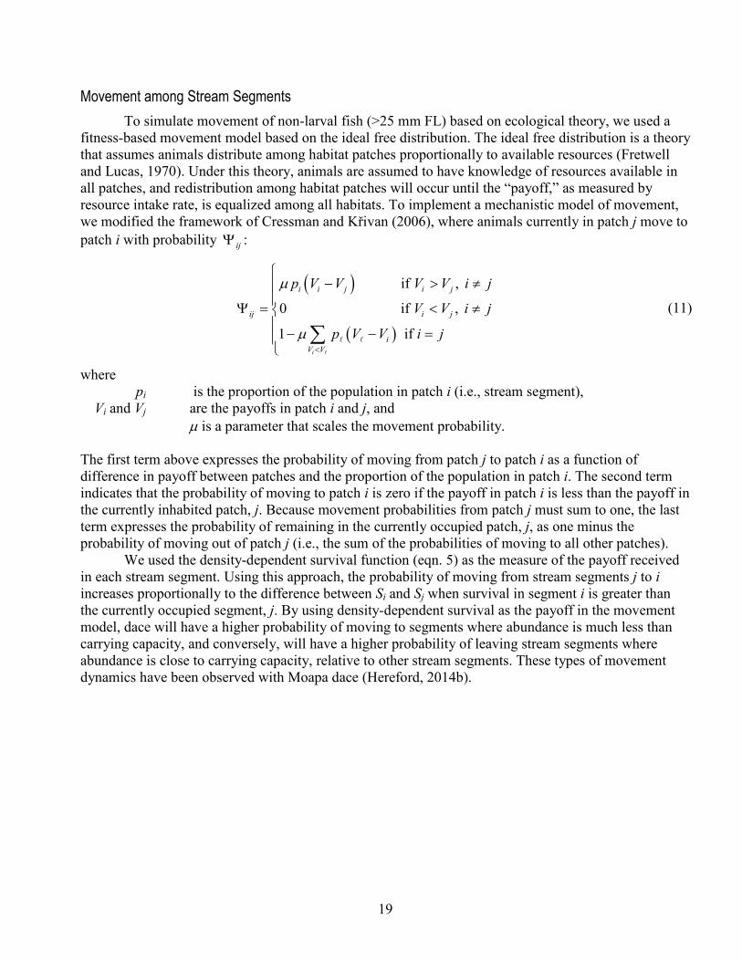
Movement among Stream Segments To simulate movement of non-larval fish (>25 mm FL) based on ecological theory, we used a

fitness-based movement model based on the ideal free distribution. The ideal free distribution is a theory that assumes animals distribute among habitat patches proportionally to available resources (Fretwell and Lucas, 1970). Under this theory, animals are assumed to have knowledge of resources available in all patches, and redistribution among habitat patches will occur until the “payoff,” as measured by resource intake rate, is equalized among all habitats. To implement a mechanistic model of movement, we modified the framework of Cressman and Křivan (2006), where animals currently in patch j move to patch i with probability ijΨ :

( )

( )

if ,

0 if ,

1 if i

i i j i j

ij i j

iV V

p V V V V i j

V V i j

p V V i j<

− > ≠

Ψ = < ≠− − =

∑

m

m

(11)

where pi is the proportion of the population in patch i (i.e., stream segment), Vi and Vj are the payoffs in patch i and j, and m is a parameter that scales the movement probability. The first term above expresses the probability of moving from patch j to patch i as a function of difference in payoff between patches and the proportion of the population in patch i. The second term indicates that the probability of moving to patch i is zero if the payoff in patch i is less than the payoff in the currently inhabited patch, j. Because movement probabilities from patch j must sum to one, the last term expresses the probability of remaining in the currently occupied patch, j, as one minus the probability of moving out of patch j (i.e., the sum of the probabilities of moving to all other patches).

We used the density-dependent survival function (eqn. 5) as the measure of the payoff received in each stream segment. Using this approach, the probability of moving from stream segments j to i increases proportionally to the difference between Si and Sj when survival in segment i is greater than the currently occupied segment, j. By using density-dependent survival as the payoff in the movement model, dace will have a higher probability of moving to segments where abundance is much less than carrying capacity, and conversely, will have a higher probability of leaving stream segments where abundance is close to carrying capacity, relative to other stream segments. These types of movement dynamics have been observed with Moapa dace (Hereford, 2014b).

20

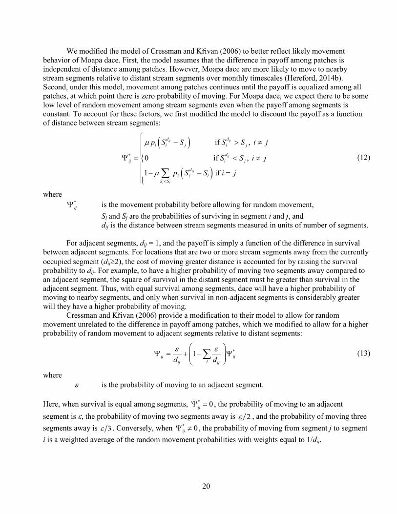
We modified the model of Cressman and Křivan (2006) to better reflect likely movement behavior of Moapa dace. First, the model assumes that the difference in payoff among patches is independent of distance among patches. However, Moapa dace are more likely to move to nearby stream segments relative to distant stream segments over monthly timescales (Hereford, 2014b). Second, under this model, movement among patches continues until the payoff is equalized among all patches, at which point there is zero probability of moving. For Moapa dace, we expect there to be some low level of random movement among stream segments even when the payoff among segments is constant. To account for these factors, we first modified the model to discount the payoff as a function of distance between stream segments:

( )

( )*

if ,

0 if ,

1 if

ij ij

ij

j

i

d di i j i j

dij i j

di

S S

p S S S S i j

S S i j

p S S i j<

− > ≠

Ψ = < ≠− − =

∑

m

m

(12)

where *

ijΨ is the movement probability before allowing for random movement, Si and Sj are the probabilities of surviving in segment i and j, and dij is the distance between stream segments measured in units of number of segments.

For adjacent segments, dij = 1, and the payoff is simply a function of the difference in survival between adjacent segments. For locations that are two or more stream segments away from the currently occupied segment (dij≥2), the cost of moving greater distance is accounted for by raising the survival probability to dij. For example, to have a higher probability of moving two segments away compared to an adjacent segment, the square of survival in the distant segment must be greater than survival in the adjacent segment. Thus, with equal survival among segments, dace will have a higher probability of moving to nearby segments, and only when survival in non-adjacent segments is considerably greater will they have a higher probability of moving.

Cressman and Křivan (2006) provide a modification to their model to allow for random movement unrelated to the difference in payoff among patches, which we modified to allow for a higher probability of random movement to adjacent segments relative to distant segments:

*1ij ijiij ijd d

Ψ = + − Ψ

∑e e (13)

where e is the probability of moving to an adjacent segment. Here, when survival is equal among segments, * 0ijΨ = , the probability of moving to an adjacent segment is e, the probability of moving two segments away is 2e , and the probability of moving three segments away is 3e . Conversely, when * 0ijΨ ≠ , the probability of moving from segment j to segment i is a weighted average of the random movement probabilities with weights equal to 1/dij.

21

To parameterize the model, we set m=0.5 and e=0.01, which resulted in a 1–3 percent probability of moving out of a given segment when survival was equal among stream segments. This level of movement approximates the movement probabilities observed based on genetic mark-recapture studies (Hereford, 2014b), although Hereford (2014b) examined movement distance over a bimonthly timescale rather than movement probabilities on a monthly timescale as implemented in our model. Barriers were represented in the model by setting the upstream and downstream movement probabilities to zero between segments separated by permanent barriers (for example, the gabion barrier). For the two barriers to upstream movements in the Pedersen system, upstream movement probabilities were set zero, but fish were allowed to move downstream of the upper and middle Pedersen segments (segments 3 and 4) according to the fitness-based movement model. However, during initial calibration of the model, we noted that populations in these segments always went extinct over the time horizon during which the population in these segments was known to persist. These findings indicated that simulated movement out of these reaches was higher than occurred in reality, suggesting that the upstream barriers in the Pedersen system also were likely impediments to downstream movement, an observation also supported by the findings of Hereford (2014b). Although genetic analysis identified the upper Pedersen population as genetically distinct, Hereford (2014a) also found evidence that individuals from upper Pedersen contributed to populations downstream of upper Pedersen, indicating that some downstream movement does occur. To reflect these patterns of movement, we reduced the random movement probability from upper and middle Pedersen by treating them as if they were separated by an additional stream segment. For example, for segments adjacent to upper and middle Pedersen, dij was increased from 1 to 2, and likewise for more distant segments.

Movement dynamics of larval Moapa dace (<25 mm FL) are completely unknown. Therefore, we used a simple movement model that assumed a low level of downstream dispersal but no upstream dispersal. We assigned an emigration probability of 3 percent per month from each stream segment and assumed that larvae could disperse by as much as two stream segments downstream per month. For stream segments that had only a single downstream segment, individuals had a 3-percent probability of moving to the downstream segment. For stream segments with two or more downstream segments, we assumed a 2-percent probability of moving to the adjacent downstream segment, and a 1-percent probability of dispersing downstream by two segments.

To implement this movement model in the stochastic IBM, we randomly drew the segment to which a fish moved by treating the stream segments as drawn from a multinomial distribution, with the probabilities of movement to each segment from a given segment forming the multinomial cell probabilities.

Model Calibration Our IBM was constructed from a combination of empirically derived parameter estimates (for

example, growth and survival), ecologically based theoretical models (for example, fitness-based movement), and assumed demographic parameters for life stages in which little is known (for example, reproduction and larval survival). Therefore, the goal of model calibration was to identify parameter values for the most uncertain model parameters that produced population trajectories consistent with the observed historical abundance of Moapa dace. The most uncertain model parameters driving population dynamics in our model were (1) the total carrying capacity of stream segments upstream of the gabion barrier (segments 1–7), (2) the carrying capacity of the mainstem Muddy River and associated tributaries downstream of the gabion barrier (segment 8), and (3) survival of larvae from an egg in a reproductive female to the point at which larvae transition to juveniles at 25 mm FL.

22

To calibrate the model, we varied carrying capacity and larval survival, ran the model for a 30-year period, and then evaluated the goodness of fit of simulated population sizes relative to the historical time series of population estimates based on annual and bi-annual snorkel censuses extending back to 1985. The snorkel surveys primarily count juvenile and adult dace. We eliminated larval counts where larvae were noted in the snorkel survey data owing to likely low detection probabilities of larvae. We then compared simulated non-larval abundance to the snorkel census data. Therefore, all population trajectories presented in this report exclude larvae and represent only abundance of juvenile and adult Moapa dace.

As our measure of goodness of fit to observed data, we used a negative log-likelihood function that assumed a multiplicative lognormal distribution of errors between observed and simulated abundance. First, we assumed the following model for the observed population size:

( )obs, sim, expt t tN N= e , (14)

( ) ( )obs, sim,ln lnt t yN N= + e where obs,tN is the observed number of non-larval Moapa dace at time t from the snorkel census, sim,tN is the simulated number of non-larval dace at time t, and

( )2Normal 0,te σ is an additive error term on the logarithmic scale. The negative log-likelihood for this model is:

( ) ( ) ( ) 2

obs, sim,obs, 2

ln ln1ln | ln exp22

t tt

t

N NL N

− − = − − ∑θ

σσ p (15)

where ( )obs,ln | tL Nθ− is the negative log-likelihood of the parameters (θ) given the observed data ( obs,tN ).

The residual standard deviation, σ, can be estimated analytically using:

( ) ( ) 2

obs, sim,1

1ˆ ln lnn

t ty

N Nn =

= − ∑σ . (16)

23

Because the IBM is a stochastic model that produces a different population trajectory on each run, we used the method of simulated maximum likelihood, which estimates the expected value of the likelihood over an ensemble of stochastic model runs (Gouriéroux and Monfort, 1997). In this case, the likelihood function (eqn. 15) is replaced with:

( ) ( ) ( ) 2

obs, sim, ,obs, 2

1

ln ln1 1ˆln | ln exp22

S t t st

t s ss

N NL N

S =

− − = − −

∑ ∑θσσ p

(17)

where s = 1, …, S stochastic realizations of the IBM, and L̂ denotes that this function estimates the expected value of the likelihood function over

S stochastic realizations. We set S=100, meaning that we ran 100 stochastic realizations of the IBM for each set of parameter values, and calculated ( )obs,

ˆln | tL Nθ− based on these 100 realizations. We used the likelihood function described in equation 17 to evaluate the relative goodness of fit

to observed data for alternative combinations of parameter values. Lower values of the negative log-likelihood function indicate parameter values that result in a better fit of the simulated population trajectories to observed data. Because all alternative parameter sets involved varying the same number of parameters, twice the negative log likelihood (hereafter referred to as “NLL”) is equivalent to model selection criterion known as Akaike’s Information Criterion (AIC; Burnham and Anderson, 2002). A difference of AIC ≤ 2 among models indicates competing models that fit the data equally well. Therefore, we interpreted differences of ≤ 1 NLL as parameter sets that fit the observed data equally well. Our goal then was to select sets of parameter values that were within one unit of the minimum NLL.

We performed model calibration in two stages. In the first stage, the goal was to estimate larval survival and the total carrying capacity of all stream segments upstream of the gabion barrier (segments 1–7). Therefore, we first fit the model to the time series of abundance estimates after the gabion had been installed by 1997 when movement of fish between the mainstem and tributaries upstream of the gabion was eliminated. Although the population upstream of the gabion barrier represented nearly the entire Moapa dace population, residual counts of dace downstream of the gabion barrier were subtracted so that the model was fit to the population size upstream of the gabion barrier. We selected three values of monthly larval survival (Slarvae = {0.25, 0.30, 0.35}). For each value of Slarvae, we ran the model over a range of total carrying capacity for all stream segments upstream of the gabion barrier. Total carrying capacity ranged from 4,200 to 11,000, a range that was wide enough to encompass the minimum NLL for each value of Slarvae. Because the probability of an egg being laid (plaid) and hatched (phatched) was unknown, these parameters were set to 1. Therefore, Slarvae represents the average monthly probability that an egg in a reproductive female is laid, hatched, and survives to the juvenile stage, at which point it becomes available to be counted in the snorkel survey data to which the model is fit (see eqn. 3). We then selected a value of Slarvae and carrying capacity among all parameter sets that were within 1 unit of the minimum NLL.

24

For the second stage of calibration, the goal was to estimate the carrying capacity of the mainstem Muddy River and tributaries downstream of the gabion barrier (segment 8). Thus, we fit the model to the observed snorkel counts from 1985to 1995, the period before tilapia were introduced when Moapa dace inhabited the mainstem and moved freely between the mainstem and segments 1–7 upstream of the gabion barrier. For this calibration, we fixed Slarvae and carrying capacity upstream of the gabion barrier to the best-fit value from the first stage of calibration, and then estimated carrying capacity downstream of the gabion barrier (segment 8) by fitting the model to the total population abundance both upstream and downstream of the gabion barrier. We fit the model to the total population abundance rather than just abundance in segment 8 because presence of larger fish and movement of fish between the mainstem and tributaries could influence the total population size upstream and downstream of the gabion despite no change in capacity for segments 1–7. Therefore, fitting only to abundance estimates downstream of the gabion barrier may have underestimated its capacity. Carrying capacity of segment 8 ranged from 9,000 to 16,000. We then selected the carrying capacity for segment 8, which minimized the NLL of total population abundance. These values of Slarvae and total carrying capacity upstream and downstream of the gabion barrier were then used in all model runs to evaluate alternative scenarios.

Calibration also required that the population model attain a stable equilibrium before comparing simulated to observed data. To minimize the time required to reach equilibrium, we used an initial population of individuals that was sufficiently close to the equilibrium population structure. This initial population structure at time zero was obtained by (1) selecting parameter values that approximately matched observed population sizes, (2) running the model for 18 years to allow the population to attain equilibrium, and then (3) using the simulated population of individuals at year 18 as the initial population for all parameter sets in the calibration. We determined that a “burn in” of 5 years allowed population trajectories to reach equilibrium under a wide range of parameter values. Thus, simulated population trajectories were compared to observed abundances, beginning in year 6, after allowing population trajectories to reach equilibrium.

Alternative Scenarios We ran a number of scenarios relating to migration barriers and changes to carrying capacity.

For each scenario, we ran 100 stochastic realizations of the calibrated IBM over a 50-year time horizon. Initial populations for these scenarios were developed by running 100 realizations of the calibrated model, either with or without the gabion barrier in place, for a sufficiently long time horizon to attain an equilibrium population size, spatial distribution, and life stage structure. The population of individuals at the end of this time series was then used to form the initial populations for the 100 stochastic realizations for each scenario. Depending on the scenario, initial population size ranged from 10 to 500 non-larval individuals. Here, a specified number of non-larval individuals was randomly drawn from each of the 100 initial populations. Larval Moapa dace also were randomly drawn from the initial populations in proportion to the ratio of abundance of larval to non-larval dace. On average, there was a 7-to-1 ratio of larval to non-larval dace. Although we focus our analysis and calibration on non-larval abundance, an initial population size of 10 dace, for instance, indicates that 10 non-larval dace and 70 larval dace, on average, were drawn at random from each of the 100 initial populations.

25

Migration Barriers Use of migration barriers has been an important management tool in the Warm Springs Area to

manage the spread of invasive species, yet migration barriers also may negatively affect metapopulation dynamics of Moapa dace by restricting dispersal. Over the past 20 years, the primary migration barriers were the gabion barrier in the lower Plummer stream and two weirs that prevent upstream movement into Pedersen stream. The gabion barrier separates segments 7 and 8 (fig. 2) and eliminates upstream and downstream movement. The weirs on Pedersen stream separate segments 3 from 4 and 4 from 6, and are complete barriers to upstream movement and partial barriers to downstream movement (Hereford, 2014b; fig. 2). We evaluated the effect of four alternative migration barrier scenarios to understand how migration barriers influence population dynamics. These scenarios were comprised of:

A. Baseline—all barriers in place as the stream network system has been historically configured.

B. Gabion in, Pedersen weirs out—complete removal of Pedersen weirs allowing both upstream and downstream dispersal.

C. Gabion out, Pedersen weirs in—complete removal of gabion barrier allowing both upstream and downstream dispersal.

D. Gabion out, Pedersen weirs out—removal of all barriers to movement

Carrying Capacity Many management actions and human influences affect carrying capacity. Habitat restoration

increases capacity, whereas changes in spring discharge affect carrying capacity by altering the amount of suitable habitat for Moapa dace (Hatten and others, 2013). Because carrying capacity in our model has a temporal component representing monthly capacity (fig. 5), the population size that can be supported over the long term (i.e., the equilibrium population size) may not be directly proportional to carrying capacity. Furthermore, equilibrium population size will be a complex function of not only segment-specific capacity, but also of stream network structure, movement, growth, and survival.

To understand how changes in carrying capacity affect equilibrium population sizes, we ran a series of scenarios that both increased and decreased carrying capacity. These scenarios followed the approach of Hatten and others (2013), who simulated the amount of suitable habitat resulting from changes in discharge of -30 to +30 percent in headwater springs (segments 1, 3, and 5 in our model). Similarly, our approach was to vary the total carrying capacity upstream of the gabion barrier from -30 to +30 percent in increments of 10 percentage points. Changes in carrying capacity were performed under the baseline scenario, with the gabion barrier and Pedersen weirs in place and no Moapa dace in the mainstem Muddy River (segment 8). Our goal here was to understand how changes in carrying capacity from the historical state of the system could affect, either positively or negatively, the magnitude of the equilibrium population size that the system could support.

26

Results Calibration and Model Behavior

The first stage of our model calibration exercise was informative about combinations of larval survival and carrying capacity upstream of the gabion barrier that best fit observed abundances of Moapa dace. For each value of larval survival, the negative log likelihood (NLL) followed a parabolic function of carrying capacity, with a clear range of values that were within 1 NLL of the minimum value (fig. 8). For example, for larval survival of 0.35, a carrying capacity of about 6,000 minimized the NLL, but values of capacity ranging from about 5,500 to 7,000 were within 1 NLL of the minimum value, indicating that a wide range of carrying capacity fit the observed data nearly as well. We also determined that, as larval survival decreased, a higher carrying capacity was required to obtain a similar fit to the data. For example, for monthly larval survivals of 0.25, 0.30, and 0.35, carrying capacities that were near the minimum NLL were 9,000, 7,200, and 6,000, respectively (fig. 8). Among the three values of larval survival, there was no clear global minimum. This finding indicates that larval survival was confounded with carrying capacity because alternative combinations of larval survival and carrying capacity fit the data nearly equally well. For this reason, we selected a larval survival of 0.30 at a carrying capacity of 7,200 upstream of the gabion barrier for the second stage of calibration and for simulation of all alternative scenarios.

For the second stage of calibration where we estimated capacity of the mainstem Muddy River and tributaries downstream of the gabion barrier (segment 8), we observed the minimum NLL at a carrying capacity of 13,800 (fig. 8). However, because we fit the model to only four abundance estimates that were available prior invasion of blue tilapia, there was more uncertainty in the best fit capacity, as indicated by the wide range of carrying capacities that were within 1 NLL of the minimum. Thus, carrying capacities from 11,500 to 15,500 also were plausible values. Given the selected values of larval survival (0.30) and carrying capacity (7,200 upstream of the gabion barrier and 13,800 downstream of the gabion barrier), our calibration indicated that the capacity of the mainstem Muddy River and tributaries downstream of the gabion barrier was nearly twice the capacity of the stream segments upstream of the gabion barrier.

27

Figure 8. Negative log-likelihood profiles as a function of carrying capacity. The individual-based model was fit to abundance estimates, 1997–2014 (top panel) and 1985–1995 (bottom panel). Filled symbols indicate the parameter values that were selected for all subsequent simulations.

28

Given our selected parameters of larval survival and capacity, we examined the IBM’s goodness of fit to total population abundance. For 1997–2014 when the gabion barrier was in place, the model captured the average abundance well, but failed to match the variation in observed abundance, particularly for the more recent abundance estimates after 2008 (fig. 9). Our model assumed that carrying capacity and larval survival were constant over the 20-year period, which is why the simulated trajectories fluctuate around a constant average value of about 875 individuals. However, substantial changes to the stream network occurred following 2008, including targeted removal of invasive fishes and numerous restoration activities. These actions likely had some influence on larval survival and carrying capacity. We expand on this topic in the section, “Discussion.”

For 1985–1995, the simulated population trajectories matched the observed data well, particularly when considering the run-to-run variation observed among the 100 replicate simulations (fig. 9). For example, although the mean simulated abundance fluctuated from about 2,700 to 3,300 non-larval dace, the individual realizations ranged from about 2,300 to 4,000 individuals. The simulated range of abundance matched the observed variation in snorkel counts.

Comparing the observed to simulated abundance also reveals model behavior that is not apparent in the observed abundance estimates. Population trajectories show a seasonal cycle that is not seen in the observed abundance estimates. This seasonal cycle is driven by reproduction that peaks during spring and declines to a minimum during the winter. The peaks and troughs in non-larval abundance are driven by a combination of (1) seasonal recruitment of larvae that grow large enough to transition to juveniles (>25 mm FL), and (2) density-dependent survival that reduces survival when a large pulse of larvae recruit to juveniles and begin to compete for resources with non-larval dace. Cycles are not clearly evident in the observed data because snorkel surveys have been conducted at 6-month or longer intervals, making it difficult to observe fluctuations that occur at finer scales (for example, monthly).

29

Figure 9. Graphs showing 100 population trajectories from the individual-based model (gray lines) and the mean abundance (black lines) shown against the observed snorkel counts (solid pink circles) using calibrated parameters with a larval survival rate of 0.30 at a carrying capacity of 7,200 upstream of gabion barrier and a carrying capacity of 13,800 downstream of gabion barrier. The upper panel is limited to the population upstream of the gabion barrier. The lower panel shows the total population upstream and downstream of the gabion barrier.

30

To further examine model behavior, we simulated the entire historical times series of the Moapa dace population using our best fit parameters of larval survival and carrying capacity, and then compared it to the observed data. For this simulation, we allowed fish to move freely between segments 1–7 and segment 8 until 1996. In 1996, we “installed the gabion barrier” by setting upstream and downstream movement probabilities to zero between segments 7 and 8. For the period after 1996, survival in segment 8 was set to zero to emulate the effect of the blue tilapia invasion. This simulation followed the observed population trajectory well, showing how the model can be used to simulate alternative scenarios such as past events that occurred in the Muddy River system (fig. 10).

Additionally, this simulation indicated that after the initial population decline owing to tilapia invasion, the simulated population continued to decline from about 1,200 to 800 individuals between 1996 and 2001. Our model hypothesized that fish inhabiting the mainstem Muddy River grew faster and attained larger size than fish in segments 1–7 upstream of the gabion barrier (fig. 7). Large fish that had moved from the mainstem into segments 1–7 were still present in the simulated population upstream of the gabion barrier at the time the barrier was installed in 1996. These large, highly fecund fish produced more larvae per individual, resulting in maintenance of a larger population size upstream of the gabion barrier. However, over time these larger fish died out, resulting in a gradual decline in the total population size as the population structure shifted to a population comprised of smaller adults that produced fewer larvae per individual.

Figure 10. Graph showing 100 population trajectories from the individual-based model (gray lines) and mean abundance (black line) shown against the observed snorkel counts (solid pink circles) using calibrated parameters with a larval survival rate of 0.30 at a carrying capacity of 7,200 upstream of gabion barrier and a carrying capacity of 13,800 downstream of gabion barrier. This scenario simulated the invasion of blue tilapia and installation of the gabion barrier in 1996.

31

Migration Barrier Scenarios The mean population size at equilibrium varied among the four migration barrier scenarios and

depended on the initial population size for some scenarios. For the baseline scenario (Pedersen weirs and gabion barrier in place), the mean population size at equilibrium increased as initial population size increased from 10 to 50 to 500 individuals (figs. 11 and 12). This difference also was apparent for weirs in place with the gabion barrier removed, although the relative magnitude of this difference was less (figs. 11 and 12). In contrast, for the two scenarios where the Pedersen weirs were removed, we found no effect of initial population size on the equilibrium population size (figs. 11 and 12). The primary effect of removing the gabion barrier was to allow access between three springheads (collectively, segments 1–7 in this study) and the mainstem Muddy River downstream of the gabion, which increased the equilibrium population size considerably, as would be expected.

Figure 11. Time-series of mean monthly population abundance showing differences in the equilibrium population size among four alternative scenarios of migration barriers. Mean monthly abundance was computed from 100 simulations at three initial population sizes (N0=10, 50, and 500), for each of the alternative scenarios. The upper left panel shows the baseline scenario.

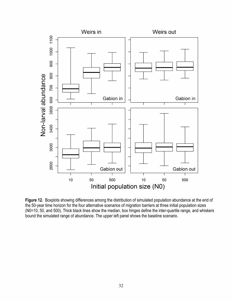
32

Figure 12. Boxplots showing differences among the distribution of simulated population abundance at the end of the 50-year time horizon for the four alternative scenarios of migration barriers at three initial population sizes (N0=10, 50, and 500). Thick black lines show the median, box hinges define the inter-quartile range, and whiskers bound the simulated range of abundance. The upper left panel shows the baseline scenario.

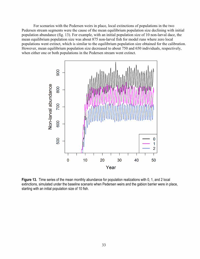
33

For scenarios with the Pedersen weirs in place, local extinctions of populations in the two Pedersen stream segments were the cause of the mean equilibrium population size declining with initial population abundance (fig. 13). For example, with an initial population size of 10 non-larval dace, the mean equilibrium population size was about 875 non-larval fish for model runs where zero local populations went extinct, which is similar to the equilibrium population size obtained for the calibration. However, mean equilibrium population size decreased to about 750 and 650 individuals, respectively, when either one or both populations in the Pedersen stream went extinct.

Figure 13. Time series of the mean monthly abundance for population realizations with 0, 1, and 2 local extinctions, simulated under the baseline scenario when Pedersen weirs and the gabion barrier were in place, starting with an initial population size of 10 fish.

34

We observed no local population extinctions with the Pedersen weirs removed, but a high probability of local extinctions at low initial population sizes when the weirs were in place. At an initial population size of 10 with weirs in place, the probability of local extinction was >80 percent (fig. 14). Even at an initial population size of 50 non-larval dace (and about 350 larval dace), the probability of at least one local extinction was about 40 percent. However, as initial population size increased to more than 100 non-larval dace, no further local extinctions were observed (fig. 14).

Figure 14. Probability of a local extinction as a function of initial population size. The two lines show the probability of one or more of the subpopulations in Pedersen stream going extinct compared to both segments going extinct.

35

Without the weirs, strong compensatory mechanisms act to buffer against local extinctions. First, at low initial population sizes, there is little intraspecific competition, which acts to increase survival. Second, even when stochastic events cause a sub-population to go extinct, the fitness-based movement function would act to increase the probability of an individual recolonizing a vacant segment, as long as individuals could freely move among segments. However, with barriers to upstream movement, once a population upstream of a barrier goes extinct, (natural) recolonization is impossible.

We also observed differences in the size and life-stage distributions among scenarios, particularly for scenarios with the gabion barrier in or out (tables 3 and 4). With access to the mainstem where fish grew faster and attained large size, the fraction of the population >65 mm FL increased (table 3), as did the abundance of fish >65 mm FL. The reproductive contribution of these large fish was disproportionate relative to their abundance. With the gabion barrier in place and no fish in the mainstem, there were about 7 larvae per adult, but this increased to about 10 larvae per adult with the gabion removed (table 4) when large fish could contribute to reproduction.

Table 3. Mean proportion of the population in each life stage in December of the last time step for four alternative scenarios of migration barriers. [Mean standard deviation is shown in parentheses. Scenario:A, baseline with weirs in and gabion barrier in; B, weirs out and gabion barrier in; C, weirs in and gabion barrier out; D, weirs out and gabion barrier out. <, less than; >, greater than; mm, millimeter]

Scenario Larvae (<25 mm FL) Juvenile (25–40 mm FL) Adult (40–65 mm FL) Adult (>65 mm FL) A 0.839 (0.0323) 0.041 (0.0095) 0.094 (0.0187) 0.026 (0.0052) B 0.839 (0.0343) 0.041 (0.0102) 0.094 (0.0198) 0.026 (0.0056) C 0.872 (0.0174) 0.042 (0.0064) 0.052 (0.0071) 0.034 (0.0046) D 0.876 (0.0174) 0.041 (0.0064) 0.051 (0.0072) 0.032 (0.0044)

Table 4. Mean population abundance in each life stage in December of the last time step for four alternative scenarios of migration barriers. [Mean standard deviation is shown in parentheses. Scenario: A, baseline with weirs in and gabion barrier in; B, weirs out and gabion barrier in; C, weirs in and gabion barrier out; and D weirs out and gabion barrier out. FL, fork length; ≤, less than or equal to; >, greater than]

Scenario Larvae Juvenile Adult

(≤ 65 mm FL) Adult

(>65 mm FL) Larvae per adult A 4,527 (1,088.221) 222 (22.367) 510 (30.786) 140 (11.827) 6.96 (1.597) B 4,577 (1,023.136) 225 (25.901) 515 (29.624) 141 (14.607) 6.97 (1.464) C 20,546 (3,169.803) 986 (74.115) 1,231 (74.263) 795 (43.652) 10.14 (1.486) D 21,381 (,3350.573) 991 (68.610) 1,238 (73.613) 786 (53.158) 10.57 (1.581)

36

Carrying Capacity Scenarios We observed that increasing or decreasing carrying capacity upstream of the gabion barrier

resulted in concomitant changes in equilibrium population size (fig. 15). For example, decreasing carrying capacity by 30 percent reduced mean abundance from about 875 to 600 individuals, but increasing capacity by 30 percent increased mean abundance to about 1,150 individuals. These changes in abundance were directly proportional to the change in carrying capacity. For example, a 30-percent decrease in capacity lead to a 30-percent decrease in mean population size.

Figure 15. Boxplots showing distribution of population sizes at the end of 50-year simulations under the baseline scenario for 100 runs of the individual-based model. The baseline scenario consisted of the gabion barrier and Pedersen weirs in place. Carrying capacity varied in 10-percentage-point increments from the baseline carrying capacity of 7,200. Thick black lines show the median, box hinges define the inter-quartile range, and whiskers bound the simulated range of abundance.

37

Discussion Our population model of Moapa dace proved a useful tool for understanding how dace

populations might respond to changes in their habitat, such as alternative configuration of migration barriers and changes in carrying capacity. The IBM was constructed from a combination of empirically derived parameter estimates (for example, growth and survival), ecologically based theoretical models (for example, fitness-based movement), and assumed demographic parameters for life stages in which little is known (for example, reproduction and larval survival). Additionally, we calibrated the model to historical estimates of population abundance, which allowed us to assess scenarios that included reintroduction of dace to the mainstem Muddy River.

Because our model incorporates density-dependent processes that are driven by the capacity of available habitat to support Moapa dace, it is well suited to evaluate the potential effect of management actions that alter the amount of habitat. Changes to total capacity of tributary streams upstream of the gabion barrier led to changes in population abundance directly proportional to the change in capacity. However, we would not always expect population size to change in direct proportionality to carrying capacity. In our simulations, we simultaneously increased carrying capacity for all stream segments, which maintained the relative distribution of carrying capacity among stream segments. Because movement and survival in our model are intricately linked to the channel network structure and distribution of abundance by density-dependent relations, these relations remained unchanged when simultaneously changing capacity in all segments. However, if changes in carrying capacity had occurred disproportionately in some stream segments, we expect that the population dynamics would respond in such a way that the consequent change in total capacity could result in disproportionate changes to the total population size. Changing capacity in one segment but not others would influence the movement probabilities and the density-dependent survival relations. Thus, we should not always assume that population size would change in direct proportionality to carrying capacity. For this reason, our model could be a useful tool for examining where habitat restoration might yield higher or lower benefits to the population.

Although we examined how changes in capacity affect population size, we did not directly examine how specific factors, such as reduced spring discharge or habitat restoration, would influence population dynamics. The difficult link to make here is determining the amount by which carrying capacity would change in response to a change in spring discharge of a given magnitude. Hatten and others (2013) used detailed ecohydraulic models to show that the amount of suitable habitat for Moapa dace declined in response to reduced spring discharge of three headwater segments (segments 1, 3, and 5 in our model). However, to translate these effects to carrying capacity at the population level would require estimating how a change in spring discharge would affect the total amount of available habitat throughout all stream segments supporting the Moapa dace population. Thus, although our model is useful for understanding how changes in carrying capacity of a given magnitude might affect populations of Moapa dace, it remains a formidable challenge to mechanistically link specific types of changes in habitat (for example, reduced spring flows) to specific changes in carrying capacity.

38

In constructing our model, we were forced to make many simplifying assumptions because of the lack of knowledge about some aspects of Moapa dace biology. Chief among these assumptions was the reproductive biology of Moapa dace. We assumed that (1) individual Moapa dace spawn only once per year, (2) all eggs were laid when an individual spawned, (3) spawning occurred everywhere, and (4) larval survival was the same everywhere. All these assumptions are likely to be invalid to some extent. Anecdotal evidence based on observations of larvae suggests that successful reproduction occurs near headwater springs. However, reproduction of Moapa dace has never been observed in the wild. The frequency with which an individual spawns and how many eggs are spawned by an individual are unknown. However, by calibrating larval survival to allow the model to fit observed abundance estimates, we believe that our model captures the probability that an egg in a reproductive female survives to the juvenile stage. As more is learned about the reproductive biology of Moapa dace, we should be able to refine this aspect of the model.

Another important assumption was that growth rates of Moapa dace in the mainstem Muddy River were higher than in tributary streams. We have no direct evidence for higher growth rates except for historical observations showing that larger fish occupied the mainstem Muddy River but no longer exist in the population of Moapa dace upstream of the gabion barrier. It is possible that Moapa dace achieved larger size in the mainstem not owing to higher growth rates but because of higher survival rates that allowed them to live longer and achieve larger size. The 2014 flood event that washed out the gabion barrier offers an excellent opportunity to test these hypotheses once Moapa dace become established in their historical habitat.

Our model fit the average abundance upstream of the gabion barrier well, but clearly did not represent the magnitude of population fluctuations that occurred after 2008 (fig. 9). By estimating a single larval survival and carrying capacity, our analysis made the implicit assumption that carrying capacity and larval survival remained constant over the 20-year period. However, substantial changes to the stream network occurred following 2008. First, a sharp decline of the population to about 436 individuals occurred in 2008. To our knowledge, the cause of this decline has not been identified. Second, major restoration projects began around 2008. Upper Apcar stream was restored (segment 5), lower Pedersen stream was restored and redirected to its historical channel (segment 4), and the middle section of Apcar stream was restored (segment 6 and part of segment 7). Third, an extensive bimonthly trapping effort began in 2008 (Hereford, 2014a, 2014b) whereby invasive fishes were removed from the system, and larval dace are known to be consumed by invasive fish species (Scoppettone, 1993). Thus, carrying capacity of the stream network increased over time owing to restoration activities, and reduction of invasive fish populations may have increased larval survival and reduced competition with non-larval dace. It would have been difficult to represent the effects of these changes in our model because the ecosystem has been in a state of flux since 2008. The Moapa dace population appears to be responding positively to these recent activities. Should the population begin to stabilize at a new, higher equilibrium population size in the future, our model could be used to estimate the capacity of the stream network before and after restoration activities took place. Such an analysis could provide the basis for predicting the effects of habitat restoration in other locations, providing fisheries managers with an important tool for evaluating the effects of restoration actions on Moapa dace abundance.

39

Our simulations suggest that reintroducing Moapa dace to the mainstem Muddy River and increasing carrying capacity would result in substantial increases in Moapa dace abundance. However, our analyses suggest that these efforts alone will not be sufficient to achieve the recovery goal of 6,000 Moapa dace (U.S. Fish and Wildlife Service, 1996). Our estimate of carrying capacity for the mainstem Muddy River and tributaries represents the capacity of the system when dace abundance was estimated between 1985 and 1995. During 1985–1995, available habitat already was reduced, and the Muddy River and its tributaries likely have changed since 1995. To achieve the recovery goal, our analyses suggest that carrying capacity needs to be increased further by continued restoration of existing habitats and reintroductions to habitats from which dace have been extirpated. Our model could be a useful tool to help understand the magnitude of change in carrying capacity required to meet recovery goals. For example, it would be straightforward to explicitly represent other spring tributaries that connect to the mainstem Muddy River (for example, Cardy Lamb Springs). Based on our analysis of carrying capacity in other areas, we could hypothesize the increase in capacity achieved by reintroducing Moapa dace to additional headwater springs, and the consequent effect on the expected equilibrium abundance.

Acknowledgments The culmination of efforts required to develop this individual-based model is impressive, and

there are many people deserving of thanks that we never had the chance to meet. This was a team effort all the way, and represents decades of research. We owe a great deal of gratitude to our sponsor and U.S. Fish and Wildlife Service (USFWS) liaison Lee H. Simons, who nurtured this endeavor. Dave Syzdek and the Southwest Nevada Water Authority are appreciated for the access, resources, and enthusiasm they have provided in ongoing research. We are grateful for the roundtable meetings of the Biological Advisory Committee, and the passionate and diverse group of people that participated. We thank our U.S. Geological Survey (USGS) colleagues in the Reno, Nevada, office, including Peter Rissler and Mark Fabes for their support. We thank local USGS personnel at the Columbia River Research Laboratory for providing the necessary computer crunching power during their off time. We also thank James Hatten and Thomas Batt for geographic information system assistance. Graduate students Danielle Hereford and Mark Hereford deserve special thanks for the invaluable data provided that informed our models, and their insights that can only be gained by long hours of field and lab work. This study was funded under USFWS Agreement Number PR40032428.

40

References Cited Beverton, R.J.H., and Holt, S.J., 1957, On the dynamics of exploited fish populations: London, Chapman

and Hall, 533 p. Burnham, K.P., and Anderson, D.R., 2002, Model selection and multimodel inference—A practical

information-theoretic approach: New York, Springer, 488 p. Burnham, K.P., and White, G.C., 2002, Evaluation of some random effects methodology applicable to bird

ringing data: Journal of Applied Statistics, v. 29, p. 245–264. Cressman, R., and Křivan, V., 2006, Migration dynamics for the ideal free distribution: The American

Naturalist, v. 168, p. 384–397. Francis, R.I.C.C., 1988, Maximum likelihood estimation of growth and growth variability from tagging data:

New Zealand Journal of Fisheries and Aquatic Science, v. 22, p. 42–51. Fretwell, D.S., and Lucas, 1970, On territorial behavior and other factors influencing habitat distribution in

birds: Acta Biotheoretica, v. 19, p. 16–32. Gouriéroux, C., and Monfort, A., 1997, Simulation-based econometric methods: Oxford, United Kingdom,

Oxford University Press, 192 p. Hatten, J.R., Batt, T.R., Scoppettone, G.G., and Dixon, C.J., 2013, An ecohydraulic model to identify and

monitor Moapa dace habitat: PLoS ONE, v. 8, no.2, 12 p., doi:10.1371/journal.pone.0055551. Hereford, M.E., 2014b, Home range, spatial dynamics, and growth of Moapa dace (Moapa coriacea); Reno,

University of Nevada, Master’s thesis, 70 p. Hereford, D.M., 2014a, Population genetics and population dynamics of Moapa dace: Reno, University of

Nevada, Master’s thesis, 131 p. Mayer T.D., and Congdon, R.D., 2008, Evaluating climate variability and pumping effects in statistical

analyses: Ground Water, v. 46, p. 212–227. Moussalli, E., and Hilborn, R., 1986, Optimal stock size and harvest rate in multistage life history models:

Canadian Journal of Fisheries and Aquatic Sciences, v. 43, p. 135–141. Quinn, T.J., and Deriso, R.B., 1999, Quantitative fish dynamics: New York, Oxford University Press, 542 p. Royle, J.A., 2004, N-mixture models for estimating population size from spatially replicated counts:

Biometrics v. 60, p. 108–115. Scoppettone, G.G., 1993, Interactions between native and nonnative fishes of the upper Muddy River,

Nevada: Transactions of the American Fisheries Society, v. 122, p. 599–608. Scoppettone, G.G., and Burge, H.L., 1994, Growth and survivorship of Moapa dace (Osteichthys,

Cyprinidae, Moapa coriacea) in an isolated stream reach on Moapa National Wildlife Refuge: Southwestern Naturalist, v. 39:, p. 92–195.

Scoppettone, G.G., Burge, H.L., and Tuttle, P.L., 1992, Life history, abundance, and distribution of Moapa dace (Moapa coriacea): Great Basin Naturalist, v. 52, p. 216–225.

Scoppettone ,G.G., Salgado, J.A., and Nielsen, M.B. ,2005, Blue tilapia (Oreochromis aureus) predation on fishes in the Muddy River system, Clark County, Nevada: Western North American Naturalist, v. 65, p. 410–414.

Udall, S.L., 1967, Native fish and wildlife—Endangered species: Federal Register, v. 32, no.48, p. 4,001. U.S. Department of the Interior, 1973, Threatened wildlife of the United States: U.S. Bureau of Sport

Fisheries and Wildlife Resources Publication 114. U.S. Fish and Wildlife Service, 1996, Recovery plan for the rare aquatic species of the Muddy River

ecosystem: U.S. Fish and Wildlife Service, Portland, Oregon, 60 p. White, G.C., and Burnham, K.P., 1999, Program MARK—Survival estimation from populations of marked

animals: Bird Study, v. 46, Supplement 001, p. 120–138.

41

Appendix A. Estimating Moapa Dace Growth Parameters Growth of Larval Moapa Dace

To estimate larval growth, we obtained size-at-age from a study conducted in 1984 (Scoppettone and Burge, 1994). In this study, 140 larval dace were discovered in a concrete irrigation channel, and then transported to an isolated segment of Upper Plummer Spring where their fork lengths were measured every 3 months for 3 years. We estimated length at age t, L(t), using the following form of the von Bertalanffy growth model (Quinn and Deriso, 1999):

( ) ( )( )01 k t tL t L e− −∞= − , (A1)

where t is age in months, L∞ is the asymptotic theoretical maximum fork length (mm), k is a constant of the growth rate, and t0 is the hypothetical age when L=0. For model fitting purposes, all fish were assumed to be 1 week old (t=0.25 month) at the time of first measurement. Parameter estimates were obtained by using a non-linear least-squares regression (table A1, fig. A1).

Table A1. Parameter estimates for the von Bertalanffy model fit to data from Scoppettone and Burge (1994).

Parameter Estimate Standard error L∞

56.85 1.175

k 0.120 0.007

0t -1.173 0.119

42

Figure A1. The von Bertalanffy growth model fit to size-at-age data from Scoppettone and Burge (1994). Dashed lines show 95-percent confidence intervals. Fork length in is millimeters (mm).

Growth of Juvenile and Adult Moapa Dace We analyzed size data obtained by Hereford (2014b), where juvenile and adult individuals were

trapped with minnow traps over a 3-year period in all stream segments upstream of the gabion barrier. We used the methods of Francis (1988) to fit a von Bertalannfy growth model where the response is the change in length as a function of initial length and time between recaptures:

( )( )1 k ttL L L e− ∆

∞∆ = − − (A2)

where L∆ is the change in fork length (mm) between recaptures, Lt is the initial fork length at time t, t∆ is the time between recaptures (months), L∞ is the asymptotic theoretical maximum fork length (mm), and k is a constant of the growth rate. This model was fit to 1,359 growth observations from 615 unique individuals ranging in size from 23 to 86 mm (Hereford, 2014b).

43

To determine whether fish in headwater spring segments (upper Plummer, upper Pedersen, and upper Apcar) had different growth rates than fish in downstream segments, we fit models that compared the following hypotheses:

Model 1—Both L∞ and k differed between upper and lower segments. Model 2—k differed between segments, but L∞ was the same between segments.

Model 3—No difference in L∞ or k for fish captured in upper and lower stream segments.

Fish were assigned to stream segments based on their location when initial length (Lt) was measured. To fit this model to the data, we used maximum likelihood methods that assumed growth of fish

was normally distributed with mean L∆ and standard deviation σ. However, negative growth values suggested the presence of measurement error associated with measuring fish length. Additionally, the growth data indicated that σ declined as L∆ declined. Therefore, we incorporated both measurement error and alternative structures for σ to identify a model that fit both the mean change in length and the variance in the observed change in length. The following model was assumed for the observations:

predi iL L∆ = ∆ + e (A3)

where iL∆ is the ith growth observation, predL∆ is the predicted growth based on eqn. A2, and

predi iL Le = ∆ −∆ is the deviation between observed and predicted growth, which is assumed to follow a normal distribution with mean 0 and standard deviation σ.

Following the methods of Francis (1988), the total variance contributing to σ was expressed as a function of measurement error and L∆ :

( )2 2predi L s= ∆ +σ σ (A4)

where s2 is the measurement error, and ( )2

predi Lσ ∆ is the variance for the ith growth observation expressed as a function of

predL∆ .

To estimate measurement error, we assumed that negative growth in length was impossible and that all negative values of L∆ represented error in the measurement of the true length. We assumed that measurement error was normally distributed with mean zero and standard deviation s, and then estimated s by fitting a normal distribution truncated at zero to all negative observations of L∆ . The estimate of measurement error was s=1.86 mm (standard error=0.08), which appeared consistent with the data. Measurement error was set to this value in eqn. A3 when estimating the other parameters by maximum likelihood.

44

Next, we compared alternative models for the relation of iσ with predL∆ , following the methods of Francis (1988). Alternative models were fit using the model structure that assumed both L∞ and k differed between upper and lower stream segments (Model 1 referenced earlier in this section). We fit four alternative model structures:

Model 1a— i =σ υ

Model 1b) — predi Lσ υ= ∆

Model 1c— ( )pred1 Li eυσ τ ∆= −

Model 1d— predi Lτσ υ= ∆

where υ and τ are parameters to be estimated by maximum likelihood. The first model is the null model that estimates iσ as a constant, whereas the other models express iσ as a linear, exponential, or power function of predL∆ .

We compared models using Akaike’s Information Criterion (AIC; Burnham and Anderson, 2002) and selected the model with the lowest AIC score. We first selected among models fitting different variance structures (Models 1a–1d). Given the best fitting-model for the variance, we then compared Models 1–3 to assess whether growth parameters differed among stream segments.

The model expressing iσ as a power function of length (Model 1d) fit the data considerably better than the other models. Given that ∆AIC > 10 are typically considered as having essentially no support relative to the best fitting model, we used Model 1d as the basis for comparing Models 1–3 (table A2). Relative to the full model (Model 1), a model with the same k but different L∞ was not supported (∆AIC=65.1), but the model with different k and the same L∞ fit better than the full model (∆AIC=1.7; table A3). The findings indicate that juvenile and adult Moapa dace upstream of the gabion barrier had the same asymptotic size (L∞), but that non-larval fish in headwater stream segments grew at a slower rate than non-larval fish in stream segments downstream of the headwater segments (table A4, fig. A2).

45

Table A2. Model selection results for assessing alternative variance structures for growth of Moapa dace. [NLL, Negative Log Likelihood; AIC, Akaike’s Information Criterion; ∆AIC, the difference in AIC of each model relative to the lowest-AIC mode.]

Model Number of parameters NLL AIC ∆AIC 1a 5 3851.7 7,713.5 274.3 1b 5 3746.7 7,503.5 64.3 1c 6 3755.9 7,523.7 84.5 1d 6 3713.6 7,439.2 0.0

Table A3. Model selection results for alternative hypotheses of Moapa dace growth in upper and lower stream segments using the variance structure from Model 1d. [NLL, Negative Log Likelihood; AIC, Akaike’s Information Criterion; ∆AIC, the difference in AIC of each model relative to the lowest-AIC model]

Model Number of parameters NLL AIC ∆AIC 1 6 3,713.6 7,439.2 1.7 2 5 3,713.8 7,437.5 0.0 3 4 3,748.2 7,504.3 66.8

Table A4. Parameter estimates for the best-fit model of Moapa dace growth that uses Model 1d for the variance structure and Model 2 for difference in growth rates between upper and lower stream segments.

Parameter Estimate Standard error L∞ 67.568 0.553 kupper 0.046 0.004 klower 0.064 0.003 υ 1.727 0.113 τ 0.613 0.040

46

Figure A2. Graph showing the von Bertanlanffy growth model fit to the change in length (∆L, in millimeters [mm]) between recaptures of Moapa dace in headwater and non-headwater stream segments. Solid lines show the best-fit model for headwater and non-headwater segments. Dashed lines show 95-percent confidence intervals.

Publishing support provided by the U.S. Geological SurveyScience Publishing Network, Tacoma Publishing Service Center

For more information concerning the research in this report, contact the Director, Western Fisheries Research Center

U.S. Geological Survey 6505 NE 65th Street Seattle, Washington 98115 http://wfrc.usgs.gov/

Perry and others—A

Stochastic Population Model to Evaluate M

oapa Dace Population G

rowth—

Open-File Report 2015-1126

ISSN 2331-1258 (online) http://dx.doi.org/10.3133/ofr20151126