A STRONG STABILITY CONDITION ON MINIMAL SUBMANIFOLDSAND ITS IMPLICATIONS

CHUNG-JUN TSAI AND MU-TAO WANG

Abstract. We identify a strong stability condition on minimal submanifolds that impliesuniqueness and dynamical stability properties. In particular, we prove a uniqueness theoremand a C1 dynamical stability theorem of the mean curvature flow for minimal submanifoldsthat satisfy this condition. The latter theorem states that the mean curvature flow of anyother submanifold in a C1 neighborhood of such a minimal submanifold exists for all time, andconverges exponentially to the minimal one. This extends our previous uniqueness and sta-bility theorem [26] which applies only to calibrated submanifolds of special holonomy ambientmanifolds.

1. Introduction

In our previous work [26], we study the uniqueness and C1 dynamical stability of calibratedsubmanifolds in manifolds of special holonomy with explicitly constructed Riemannian metrics.The result is extended to minimal submanifolds of general Riemannian manifolds in this paper.The assumption for the uniqueness and dynamical stability theorem is identified as a stronglystable condition which implies the stability of the minimal submanifold in the usual sense of thesecond variation of the volume functional. Recall that the mean curvature flow is the negativegradient flow of the volume functional. It is thus natural to ask whether a local minimizer (astable minimal submanifold) of the volume functional is stable under the mean curvature flow.Such a question of great generality has been addressed in the celebrated work of L. Simon [21]:when is a local minimizer dynamically stable under the gradient flow, i.e. does the gradientflow of a small perturbation of a local minimizer still converge back to the local minimizer?The question in the context of [21] concerns a nonlinear parabolic system defined on a compactmanifold, and it was proved that the analyticity of the functional and the smallness in C2

norm are sufficient for the validity of the dynamical stability. The question we addressed herecorresponds to the specialization to the volume functional of compact submanifolds. A natural

Supported in part by Taiwan MOST grants 105-2115-M-002-012, 106-2115-M-002-005-MY2 and NCTS YoungTheoretical Scientist Award (C.-J. Tsai). This material is based upon work supported by the National ScienceFoundation under Grants No. DMS-1405152 and No. DMS-1810856 (Mu-Tao Wang). Part of this work wascarried out when Mu-Tao Wang was visiting the National Center of Theoretical Sciences at National TaiwanUniversity in Taipei, Taiwan.

1

measurement of the distance between two submanifolds is the C1 (or Lipschitz) norm, in termsof which the “closeness” condition of our current result is formulated. 1

As derived in [22, §3], the Jacobi operator of the second variation of the volume functionalis (∇⊥)∗∇⊥ + R − A, where (∇⊥)∗∇⊥ is the Bochner Laplacian of the normal bundle, Ris an operator constructed from the restriction of the ambient Riemann curvature, and A isconstructed from the second fundamental form. The precise definition can be found in §3.1.A minimal submanifold is said to be strongly stable if R−A is a positive operator, see (3.2).Since (∇⊥)∗∇⊥ is a non-negative operator, strong stability implies stability in the sense ofthe second variation of the volume functional. In particular, the strong stability condition issatisfied by all the calibrated submanifolds considered in [26] which include (M denotes theambient Riemannian manifold and Σ denotes the minimal submanifold):

(i) M is the total space of the cotangent bundle of a sphere, T ∗Sn (for n > 1), with theStenzel metric [24], and Σ is the zero section;

(ii) M is the total space of the cotangent bundle of a complex projective space, T ∗CPn,with the Calabi metric [4] and Σ is the zero section;

(iii) M is the total space of one of the vector bundles S(S3), Λ2−(S

4), Λ2−(CP2), and S−(S4)

with the Ricci flat metric constructed by Bryant–Salamon [3], where S is the spinorbundle and S− is the spinor bundle of negative chirality, and Σ is the zero section ofthe respective vector bundle.

These are all metrics of special holonomy that are known to be written in a closed form, and tohave simplest non-trivial topology. Note that in all these examples, the metrics of the total spaceare Ricci flat, and the zero sections are totally geodesic. Hence, the strong stability in theseexamples is equivalent to the positivity of the operator R. In [26], we proved uniqueness anddynamical stability theorems for the corresponding calibrated submanifolds and the proofs relyon the explicit knowledge of the ambient metric, whose coefficients are governed by solutions ofODE systems. A natural question was how general such rigidity phenomenon is. In this article,we discover that the strong stability condition is precisely the condition that makes everythingwork. Moreover, we identify more examples that satisfy the strong stability condition:

Proposition A. Each of the following pairs (Σ,M) of minimal submanifolds Σ and theirambient Riemannian manifolds M satisfy the strong stability condition (3.2) :

(i) M is any Riemannian manifold of negative sectional curvature and Σ a totally geodesicsubmanifold; in particular, geodesics in hyperbolic surfaces or 3-manifolds are stonglystable;

1It was suggested by a reviewer that, since the volume functional is well-defined for varifolds, it is possible thatsome measure theoretical “closeness” condition for varifolds works for such a dynamical stability theorem. Indeed,a recent preprint by J. D. Lotay and F. Schulze “Consequences of strong stability of minimal submanifolds”(arXiv: 1802.03941) generalized our result to the setting of integral currents under the enhanced Brakke flow.

2

(ii) M is any Kähler manifold and Σ is a complex submanifold whose normal bundle haspositive holomorphic curvature.

(iii) M is any Calabi–Yau manifold and Σ is a special Lagrangian with positive Ricci cur-vature;

(iv) M is any G2 manifold and Σ is a coassociative submanifold with positive definite−2W− + s

3 on Λ2−; this is a curvature condition on g|Σ, see (3.4).

For example (i), the strong stability can be checked directly. The examples (ii), (iii), and(iv) will be explained in §3.2 and Appendix A.

We now state the main results of this paper. The first one says that a strongly stable minimalsubmanifold is rather unique.

Theorem A. Let Σn ⊂ (M, g) be a compact, minimal submanifold which is strongly stable inthe sense of (3.2). Then there exists a tubular neighborhood U of Σ such that Σ is the onlycompact minimal submanifold in U with dimension no less than n.

The second one is on the dynamical stability of a strongly stable minimal submanifold.

Theorem B. Let Σ ⊂ (M, g) be a compact, oriented minimal submanifold which is stronglystable in the sense of (3.2). If Γ is a submanifold that is close to Σ in C1, the mean curvatureflow Γt with Γ0 = Γ exists for all time, and Γt converges to Σ smoothly as t→∞.

The precise statements can be found in Theorem 4.2 (Theorem A) and Theorem 6.2 (TheoremB), respectively. For defining a measurement for the slope, the minimal submanifold Σ inTheorem B is required to be oriented. The slope measurement is based on certain extension ofthe volume form of Σ (see §2.2.4).

The C1 dynamical stability of the mean curvature flow for those calibrated submanifoldsconsidered in [26] was proved in the same paper. In this regard, this theorem is a generalizationof our previous result.

Here are some remarks on the strong stability condition. In the viewpoint of the secondvariational formula, the condition is natural, and is stronger than the positivity of the Jacobioperator. The main results of this paper are basically saying that the strong stability has nicegeometric consequences. In particular, the minimal submanifold Σ needs not be totally geodesic,while most known results about the convergence of higher codimensional mean curvature floware under the totally geodesic assumption, e.g. [30].

Note addded. One may wonder whether the stability condition already implies the dy-namical stability. More precisely, if the Jacobi operator has only positive spectrum, is theminimal submanifold Σn stable under the mean curvature flow? The answer is yes, providedone requires more on the initial condition. This was studied by Naito [18] for general negative

3

gradient flows, and by Deckelnick [7] for surface mean curvature flows in R3 with Dirichletboundary condition. The result of Naito says that if Γ is close to Σ in Hr(= L2

r) for r > n2 +2,

then the mean curvature flow Γt exists for all time, and converges to Σ in Hr as t→∞. Sincer > n

2 + 2, Hr → C2,α for some α ∈ (0, 1], and Γ is close to Σ in C2,α. Section 6.2 is added toexplain more on the results of Naito.

Acknowledgement. The authors are grateful to Prof. Gerhard Huisken for his comments onthe stability of the mean curvature flow and for pointing out the reference [7]. The authorswould like to thank Yohsuke Imagi for helpful discussions, and to thank the anonymous refereefor helpful comments on the earlier version of this paper.

2. Local geometry near a submanifold

2.1. Notations and basic properties. Let (M, g) be a Riemannian manifold of dimensionn + m, and Σ ⊂ M be a compact (embedded) submanifold of dimension n. We use ⟨·, ·⟩ todenote the evaluation of two tangent vectors by the metric tensor g. The notation ⟨·, ·⟩ is alsoabused to denote the evaluation with respect to the induced metric on Σ. Denote by ∇ theLevi-Civita connection of (M, g), and by ∇Σ the Levi-Civita connection of the induced metricon Σ.

Denote by NΣ the normal bundle of Σ in M . The metric g and its Levi-Civita connectioninduce a bundle metric (also denoted by ⟨·, ·⟩ ) and a metric connection for NΣ. The bundleconnection on NΣ will be denoted by ∇⊥.

In the following discussion, we are going to choose a local orthonormal frame e1, · · · , en,en+1, · · · , en+m for TM near a point p ∈ Σ such that the restriction of e1, · · · , en on Σ isa frame for TΣ and the restrictions of en+1, · · · , en+m is a frame for NΣ. The indexes i, j, krange from 1 to n, the indexes α, β, γ range from n + 1 to n +m, the indexes A,B,C rangefrom 1 to n+m, and repeated indexes are summed.

The convention of the Riemann curvature tensor is

R(eC , eD)eB = ∇eC∇eDeB −∇eD∇eCeB −∇[eC ,eD]eB ,

RABCD = R(eA, eB, eC , eD) = ⟨R(eC , eD)eB, eA⟩ .

What follows are some basic properties of the geometry of a submanifold. The details can befound in, for example [8, ch. 6].

(i) ∇Σ is the projection of ∇ onto TΣ ⊂ TM |Σ, and ∇⊥ is the projection of ∇ ontoNΣ ⊂ TM |Σ. Their curvatures are denoted by

RΣklij = ⟨∇Σ

ei∇Σejel −∇

Σej∇

Σeiel −∇

Σ[ei,ej ]

el, ek⟩ ,

R⊥αβij = ⟨∇⊥

ei∇⊥ejeβ −∇

⊥ej∇

⊥eieβ −∇

⊥[ei,ej ]

eβ, eα⟩ ,4

(ii) Given any two tangent vectors X,Y of Σ, the second fundamental form of Σ in M isdefined by II(X,Y ) = (∇XY )⊥, where (·)⊥ : TM → NΣ is the projection onto thenormal bundle. The mean curvature of Σ is the normal vector field defined by H =

trΣ II. With a normal vector V , II(X,Y, V ) is defined to be ⟨II(X,Y ), V ⟩ = ⟨∇XY , V ⟩.In terms of the frame,

hαij = II(ei, ej , eα) and H = hαii eα .

(iii) For any tangent vectors X,Y, Z of Σ and a normal vector V , the Codazzi equation saysthat

⟨R(X,Y )Z, V ⟩ = (∇XII)(Y, Z, V )− (∇Y II)(X,Z, V ) (2.1)

where

(∇XII)(Y, Z, V ) = X (II(Y, Z, V ))− II(∇ΣXY, Z, V )− II(Y,∇Σ

XZ, V )− II(X,Y,∇⊥XV ) . (2.2)

In terms of the frame, denote (∇eiII)(ej , ek, eα) by hαjk;i, and (2.1) is equivalent to thatRαkij = hαjk;i − hαik;j .

2.2. Geodesic coordinate and geodesic frame. For any p ∈ Σ, we can construct a “partial”geodesic coordinate and a geodesic frame on a neighborhood of p in M as follows:

(i) Choose an oriented, orthonormal basis e1, · · · , en for TpΣ. The map

F0 : x = (x1, · · · , xn) 7→ expΣp (xjej)

parametrizes an open neighborhood of p in Σ, where expΣ is the exponential map ofthe induced metric on Σ. For any x of unit length, the curve γ(t) = F0(tx) is called aradial geodesic on Σ (at p). By using ∇Σ to parallel transport e1, · · · , en along theseradial geodesics, we get a local orthonormal frame for TΣ on a neighborhood of p inΣ. The frame is still denoted by e1, · · · , en.

(ii) Choose an orthonormal basis en+1, · · · , en+m for NpΣ. By using∇⊥ to parallel trans-port en+1, · · · , en+m along radial geodesics on Σ, we obtain a local orthonormal framefor NΣ on a neighborhood of p in Σ. This frame is still denoted by en+1, · · · , en+m.It is clear that e1, · · · , en, en+1, · · · , en+m is a local orthonormal frame for TM |Σ.

(iii) The map

F : (x,y) =((x1, · · · , xn), (yn+1, · · · , yn+m)

)7→ expF0(x)(y

αeα)

parametrizes an open neighborhood of p in M . The map exp is the exponential mapof (M, g). For any y of unit length, the curve σ(t) = F (x, ty) = expF0(x)(ty) is calleda normal geodesic for Σ ⊂M .

5

(iv) For any x, step (ii) gives an orthonormal basis e1, · · · , en+m for TF (x,0)M . By using∇ to parallel transport it along normal geodesics, we have an orthonormal frame forTM on a neighborhood of p in M . This frame is again denoted by e1, · · · , en+m.

The freedom in the above construction is the choice of e1, · · · , en and en+1, · · · , en+m atp, which is O(n) × O(m). A particular choice will be made later on. When Σ is oriented,e1, · · · , en is required to form an oriented frame. In this case, the freedom is SO(n)×O(m).

Remark 2.1. We will consider the curves s 7→ expΣp (xiei+sej) and s 7→ expF0(x)(y

βeβ+seα) inthe following discussion. They will be abbreviated as F0(x+sej) and F (x,y+seα), respectively.

Remark 2.2. The frames e1, · · · , en, en+1, · · · , en+m are constructed by parallel transportalong radial geodesics on Σ and then normal geodesic for Σ. They are indeed smooth. We brieflyexplain the smoothness of e1, · · · , en on a neighborhood of p in Σ. Write ei = Sij(x)

∂∂xj . The

smoothness of the frame is equivalent to the smoothness of Sij(x). Let Γljk(x) be the Christoffel

symbols of∇Σ, i.e. ∇Σ∂

∂xj

∂∂xk = Γl

jk(x)∂∂xl . The Christoffel symbols Γl

jk(x) are smooth functions.Since ei is parallel along radial geodesics,

∇Σxl ∂

∂xlei = 0 =

(xl∂ Sij(x)

∂xl+ xlSik(x)Γ

jik(x)

)∂

∂xj.

To avoid confusion, fix ξ = (ξ1, · · · , ξn) ∈ Rn. Let γ(t) = tξ for t ∈ [0, 1]. Since ddtf(γ(t)) =

1t (x

l ∂∂xl f(x))|γ(t),

dSij(tξ)

dt= ξl Sik(tξ) Γ

jik(tξ) .

In other words, [Sij(ξ)] is the solution to the ODE system of the form dSdt = F (S, t, ξ) at t = 1,

with the identity as the initial condition. Therefore, Sij(ξ) is smooth in ξ.

2.2.1. The tubular neighborhood Uε and the distance function.

Definition 2.3. For any δ > 0, let Uδ be the image of V ∈ NΣ | |V | < δ under the exponentialmap along Σ. By the implicit function theorem, there exists ε > 0, which is determined by thegeometry of Σ and M , such that the following statements hold for Uε:

(1) The map exp : V ∈ NΣ | |V | < 2ε → U2ε is a diffeomorphism.(2) There exist the local coordinate system (x1, · · ·xn, yn+1, · · · yn+m) and the frame e1, · · · , en+m

constructed in the last subsection.(3) The function

∑α(y

α)2 is a well-defined smooth function on Uε.(4) On Uε, the square root of

∑α(y

α)2 is the distance function to Σ.(5) For any q ∈ Uε, there exists a unique p ∈ Σ such that there is a unique normal geodesic

in Uε connecting p and q.6

We now analyze the gradient of the function∑

α(yα)2. To avoid confusion, let

ξ = (ξ1, · · · , ξn) ∈ Rn and η = (ηn+1, · · · , ηn+m) ∈ Rm

be constant vectors. Consider the normal geodesic σ(t) = F (ξ, tη); its tangent vector field isσ′(t) = ηα ∂

∂yα . On the other hand, σ′(0) is also equal to ηαeα, and ηαeα is defined and parallelalong σ(t). Thus, ηα ∂

∂yα = ηαeα on σ(t). Since the y-coordinate of σ(t) is tη, we find that

yα∂

∂yα∣∣σ(t)

= tηα∂

∂yα∣∣σ(t)

= tηα eα = t σ′(t) ; (2.3)

at t = 1 it gives

yα∂

∂yα= yαeα . (2.4)

By modifying the standard geodesic argument [5, p.4–9], the vector field yα ∂∂yα |σ(t) is half of

the gradient vector field of∑

α(yα)2. In addition, note that (2.4) implies that ⟨yα ∂

∂yα , yα ∂∂yα ⟩ =∑

α(yα)2. The Gauss lemma implies that ⟨yα ∂

∂yα , sβ ∂∂yβ⟩ = 0 if

∑α y

αsα = 0. By consideringthe first variational formula of the one-parameter family of geodesics σ(t, s) = expF0(ξ+sej)(tη),one finds that ⟨yα ∂

∂yα ,∂∂xj ⟩ = 0. It follows from these relations that

∇

(∑α

(yα)2

)= 2yα

∂

∂yα. (2.5)

For a locally defined smooth function near p, the following lemma establishes its expansionin terms of the coordinate system constructed above.

Lemma 2.4. Let Uε be a neighborhood of p ∈ Σ in M as in Definition 2.3 with the coordinatesystem (x,y) = (x1, · · ·xn, yn+1, · · · yn+m) and the frame e1, · · · , en, en+1, · · · en+m. Then,any smooth function f(x,y) on Uε has the following expansion:

f(x,y) = f(0,0) + xi ei(f)|p + yα eα(f)|p +O(|x|2 + |y|2) .

More precisely, it means that∣∣f(x,y)− f(0,0)− xi ei(f)|p − yα eα(f)|p∣∣ ≤ c(|x|2 + |y|2) for

some constant c determined by the C2-norm of f and the geometry of M and Σ.

Proof. Let q ∈ Uε be any point. To avoid confusion, denote the coordinate of q by (ξ, η),where ξ ∈ Rn and η ∈ Rm are regarded as constant vectors. Let q0 ∈ Σ be the point withnormal coordinate (ξ,0), and consider the radial geodesic on Σ joining q0 and p, σ0(t) = F0(tξ).Applying Taylor’s theorem on f(σ0(t)) gives

f(ξ,0) = f(0,0) +d

dt

∣∣t=0

f(σ0(t)) +

∫ 1

0(1− t)d

2 f(σ0(t))

dt2dt .

7

Since σ′0(t) = ξi ei, we find that

f(ξ,0) = f(0,0) + ξi ei(f)|p + ξiξj∫ 1

0(1− t) (ej(ei(f)))(σ0(t)) dt . (2.6)

Next, consider the normal geodesic joining q and q0, σ(t) = F (ξ, tη). Remember that σ′(t) =ηαeα. By considering f(σ(t)),

f(ξ, η) = f(ξ,0) + ηα (eα(f))|q0 + ηαηβ∫ 1

0(1− t) (eβ(eα(f)))(σ(t)) dt . (2.7)

Similar to (2.6), (eα(f))|q0 = (eα(f))|p + ξj∫ 10 ej(eα(f))(σ0(t)) dt. Putting these together fin-

ishes the proof of this lemma.

2.2.2. The expansions of coordinate vector fields.

Lemma 2.5. Let Uε be a neighborhood of p ∈ Σ in M as in Definition 2.3 with the coordinatesystem (x,y) = (x1, · · ·xn, yn+1, · · · yn+m) and the frame e1, · · · , en, en+1, · · · en+m. Write

∂

∂xi= ⟨ ∂

∂xi, eA⟩eA and ∂

∂yµ= ⟨ ∂

∂yµ, eA⟩eA ,

then ⟨ ∂∂xi , eA⟩ and ⟨ ∂

∂yµ , eA⟩, considered as locally defined multi-indexed functions, has thefollowing expansions:

⟨ ∂∂xi

, ej⟩∣∣(x,y)

= δij − yαhαij∣∣p+O(|x|2 + |y|2) ,

⟨ ∂∂yµ

, eβ⟩∣∣(x,y)

= δµβ +O(|x|2 + |y|2) ,(2.8)

and both ⟨ ∂∂xi , eβ⟩

∣∣(x,y)

and ⟨ ∂∂yµ , ej⟩

∣∣(x,y)

are of the order |x|2+ |y|2. By inverting the matrices,

ei =∂

∂xi+ yαhαij

∂

∂xj+O(|x|2 + |y|2) and eα =

∂

∂yα+O(|x|2 + |y|2) . (2.9)

Proof. We apply Lemma 2.4 to these locally defined functions.By construction, ⟨ ∂

∂xi , ej⟩|p = δij . With a similar argument as that for (2.4), xi ∂∂xi = xiei on

Σ ∩ Uε. It follows that

xj = xℓ⟨ ∂∂xℓ

, ej⟩ .

Differentiating the above equation first with respect to xi and then with respect to xk, andthen evaluating at p which has xℓ = 0 for all ℓ, we obtain(

∂

∂xk⟨ ∂∂xi

, ej⟩)∣∣∣∣

p

+

(∂

∂xi⟨ ∂∂xk

, ej⟩)∣∣∣∣

p

= 0 .

8

On the other hand, it follows from the construction that (∇Σej)|p = 0, and(∂

∂xk⟨ ∂∂xi

, ej⟩)∣∣∣∣

p

= ⟨∇Σ∂

∂xk

∂

∂xi, ej⟩

∣∣∣∣p

= ⟨∇Σ∂

∂xi

∂

∂xk, ej⟩

∣∣∣∣p

=

(∂

∂xi⟨ ∂∂xk

, ej⟩)∣∣∣∣

p

.

Hence, ∂∂xk ⟨ ∂∂xi , ej⟩ is zero at p.

Since eA is parallel with respect to ∇ along normal geodesics and eα = ∂∂yα at p, (∇eαeA)|p =

0 = (∇ ∂∂yα

eA)|p. It follows that(∂

∂yα⟨ ∂∂xi

, ej⟩)∣∣∣∣

p

= ⟨∇ ∂∂yα

∂

∂xi, ej⟩

∣∣∣∣p

= ⟨∇ ∂

∂xi

∂

∂yα, ej⟩

∣∣∣∣p

= − ⟨ ∂∂yα

,∇ ∂

∂xiej⟩∣∣∣∣p

= −hαij∣∣p

where the third equality follows from the fact that ⟨ ∂∂yα , ej⟩ ≡ 0 on Σ ∩ Uε.

Note that ⟨ ∂∂xi , eβ⟩ vanishes on Σ ∩ Uε. Since eβ is parallel with respect to ∇ along normal

geodesics, (∇eαeβ)|p = 0, and then(∂

∂yα⟨ ∂∂xi

, eβ⟩)∣∣∣∣

p

= ⟨∇ ∂∂yα

∂

∂xi, eβ⟩

∣∣∣∣p

= ⟨∇ ∂

∂xi

∂

∂yα, eβ⟩

∣∣∣∣p

.

By construction, ∂∂yα = eα on Σ ∩ Uε and (∇⊥eα)|p = 0. Therefore, ∂

∂yα ⟨∂∂xi , eβ⟩ is zero at p.

The term ⟨ ∂∂yµ , ej⟩ also vanishes on Σ ∩ Uε. It follows from (2.4) that yµ⟨ ∂

∂yµ , ej⟩ = 0.Differentiating the above equation first with respect to yα and then with respect to yβ, weobtain (

∂

∂yα⟨ ∂∂yβ

, ej⟩)∣∣∣∣

p

+

(∂

∂yβ⟨ ∂∂yα

, ej⟩)∣∣∣∣

p

= 0 .

Since ∇eνej = 0, the above two terms are always equal to each other, and thus both vanish.For ⟨ ∂

∂yµ , eβ⟩, it follows from the construction that ⟨ ∂∂yµ , eβ⟩ = δµβ on Σ ∩ Uε. According

to (2.4), yµ = yν⟨ ∂∂yν , eµ⟩. By a similar argument as that for ∂

∂xk ⟨ ∂∂xi , ej⟩, ∂∂yν ⟨

∂∂yµ , eβ⟩ also

vanishes at p.

2.2.3. The expansions of connection coefficients.

Proposition 2.6. Let Uε be a neighborhood of p ∈ Σ in M as in Definition 2.3 with thecoordinate system (x,y) = (x1, · · ·xn, yn+1, · · · yn+m) and the frame e1, · · · , en, en+1, · · · en+m.Let

θBA = ⟨∇eCeA, eB⟩ωC = θBA(eC)ω

C

be the connection 1-forms of the frame fields on Uε, where ωAn+mA=1 is the dual coframe of

eAn+mA=1 . Then, at a point q ∈ Uε with coordinates (x,y), θBA(eC), considered as locally defined

9

multi-indexed functions, has the following expansions:

θji (ek)|(x,y) =1

2xlRΣ

jilk

∣∣p+ yαRjiαk

∣∣p+O(|x|2 + |y|2) ,

θji (eβ)|(x,y) =1

2yαRjiαβ

∣∣p+O(|x|2 + |y|2) ,

(2.10)

θαi (ej)|(x,y) = hαij∣∣p+ xk hαij;k

∣∣p+ yβ (Rαiβj +

∑k

hαikhβjk)∣∣p+O(|x|2 + |y|2) , (2.11)

θαi (eβ)|(x,y) =1

2yγ Rαiγβ

∣∣p+O(|x|2 + |y|2) ,

θαβ (ei)|(x,y) =1

2xj R⊥

αβji

∣∣p+ yγ Rαβγi

∣∣p+O(|x|2 + |y|2)

θαβ (eγ)|(x,y) =1

2yδ Rαβδγ

∣∣p+O(|x|2 + |y|2) ,

(2.12)

where RΣjilk

∣∣p, Rjiαk

∣∣p, Rjiαβ

∣∣phαij

∣∣p, hαij;k

∣∣p, Rαiβj

∣∣p, Rαiγβ

∣∣p,R⊥

αβji

∣∣p, Rαβγi

∣∣p, Rαβδγ

∣∣p

allrepresent the evaluation of the corresponding tensors at p and with respect to the frame fieldseini=1 and eαn+m

α=n+1.

Proof. Since the restriction of the frame eini=1 on Σ is parallel with respect to ∇Σ along theradial geodesics, xkθji (ek)

∣∣(x,0)

= 0 for any i, j ∈ 1, . . . , n. It follows that

θji (ek)∣∣(x,0)

= −xl∂ θji (el)

∂xk∣∣(x,0)

and thus θji (ek)∣∣p= 0 . (2.13)

By taking the partial derivative in xl and evaluating at p = (0,0), we find that

∂ θji (ek)

∂xl∣∣p= −

∂ θji (el)

∂xk∣∣p, or equivalently, el(θ

ji (ek))|p = −ek(θ

ji (el))|p (2.14)

Similarly, since the restriction of eµn+mµ=n+1 on Σ is parallel with respect to ∇⊥ along radial

geodesics, xkθνµ(ek)∣∣(x,0)

= 0 for any µ, ν ∈ n+ 1, . . . , n+m. It follows that

θνµ(ek)∣∣p= 0 and (2.15)

el(θνµ(ek))

∣∣p= −ek(θνµ(el))

∣∣p. (2.16)

Since the frame eAn+mi=1 is parallel with respect to ∇ along normal geodesics, yµθBA(eµ) = 0

and it follows that

θBA(eµ) = −yν∂ θBA(eν)

∂yµ⇒ θBA(eµ)

∣∣(x,0)

= 0. (2.17)

By taking partial derivatives,

∂ θBA(eµ)

∂xk= −yν

∂2 θBA(eν)

∂xk∂yµand ∂ θBA(eµ)

∂yν= −

∂ θBA(eν)

∂yµ− yδ

∂2 θBA(eδ)

∂yν∂yµ. (2.18)

10

Note that on Σ, ∂∂xi ni=1 and eini=1 are both bases for TΣ. Therefore,

ek(θBA(eµ))

∣∣(x,0)

= 0 . (2.19)

By construction, ∂∂yµ = eµ on Σ = yµ = 0 for all µ. It follows from (2.18) that

eν(θBA(eµ))

∣∣(x,0)

= −eµ(θBA(eν))∣∣(x,0)

. (2.20)

In terms of the connection 1-forms, the components of the Riemann curvature tensor are

RABCD

= ⟨∇eC∇eDeB −∇eD∇eCeB −∇[eC ,eD]eB, eA⟩

= eC(θAB(eD))− eD(θAB(eC))− (θEB ∧ θAE)(eC , eD)− θAB(eE)θED(eC) + θAB(eE)θ

EC (eD) . (2.21)

With these preparations, we proceed to prove all the expansion formulae:(The expansion of θji (ek)) It follows from (2.13) that the zeroth order term is zero. By (2.14),

the coefficient of xl in the expansion is

el(θji (ek))|p =

1

2

[el(θ

ji (ek))− ek(θ

ji (el))

]∣∣∣p=

1

2RΣ

jilk

∣∣p.

Note that for RΣαβji, all the indices of summation in (2.21) go from 1 to n. Due to (2.19), the

coefficient of yα in the expansion is

eα(θji (ek))

∣∣∣p=[eα(θ

ji (ek))− ek(θ

ji (eα))

]∣∣∣p= Rjiαk|p .

(The expansion of θji (eβ)) By (2.17), the zeroth order term is zero, and the coefficient of xl

in the expansion is zero. According to (2.20), the coefficient of yα in the expansion is

eα(θji (eβ))

∣∣∣p=

1

2

[eα(θ

ji (eβ))− eβ(θ

ji (eα))

]∣∣∣p= Rjiαβ |p .

(The expansion of θαi (ej)) On Σ ∩ Uε, θαi (ej) = ⟨∇ejei, eα⟩ = hαij . Its derivative along ek is

ek(II(ei, ej , eα)) = (∇ekII)(ei, ej , eα) + II(∇Σekei, ej , eα) + II(ei,∇Σ

ekej , eα) + II(ei, ej ,∇⊥

ekeα) .

Due to (2.13) and (2.15), the last three terms vanish at p. It follows that ek(II(ei, ej , eα))|p isequal to hαij;k|p.

The coefficient of yβ is eβ(θαi (ej))|p. By (2.19) and (2.17),

Rαiβj |p =[eβ(θ

αi (ej)) + θαi (ek)θ

kβ(ej)

]∣∣∣p= [eβ(θ

αi (ej))− hαikhβkj ]|p .

(The expansion of θαi (eβ)) According to (2.17), the zeroth order term is zero, and the coeffi-cient of xl in the expansion is zero. By (2.20) and (2.17),

eγ(θαi (eβ))|p =

1

2[eγ(θ

αi (eβ))− eβ(θαi (eγ))]|p =

1

2Rαiγβ|p .

11

(The expansion of θαβ (ei)) By (2.15), the zeroth order term vanishes. With (2.16), (2.15) and(2.13),

ej(θβα(ei))

∣∣∣p=

1

2

[ej(θ

βα(ei))− ei(θβα(ej))

]∣∣∣p=

1

2R⊥

αβji

∣∣∣p.

Note that for R⊥αβji, the index of summation in the third term of (2.21) goes from n + 1 to

n+m, and the indices of summation in the last two terms of (2.21) go from 1 to n. By (2.19),(2.17) and (2.15),

eγ(θβα(ei))

∣∣∣p=[eγ(θ

βα(ei))− ei(θβα(eγ))

]∣∣∣p= Rαβγi|p .

(The expansion of θαβ (eγ)) Due to (2.17), θαβ (eγ) vanishes on Σ∩Uε. According to (2.20) and(2.17),

eδ(θαβ (eγ))

∣∣p=

1

2

[eδ(θ

αβ (eγ))− eγ(θαβ (eδ))

]∣∣p=

1

2Rαβδγ |p .

This finishes the proof of this proposition.

2.2.4. Horizontal and vertical subspaces. For any q ∈ Uε ⊂ M , there exists a unique p ∈ Σ

such that there is a unique normal geodesic inside Uε connecting q and p. Any tensor definedon Σ can be extended to Uε by parallel transport of ∇ along normal geodesics. Here are somenotions that will be used in this paper.

Assume that Σ is oriented. The parallel transport of TΣ along normal geodesics defines ann-dimensional distribution of TM |Uε , which is called the horizontal distribution, and is denotedby H. Its orthogonal complement in TM is called the vertical distribution, and is denoted by V.It is clear that H = spane1, · · · , en and V = spanen+1, · · · , en+m. The parallel transportof the volume form of Σ along normal geodesics defines an n-form on Uε, which is denoted byΩ. Let ω1, · · · , ωn, ωn+1, · · · , ωn+m be the dual coframe of e1, · · · , en, en+1, · · · , en+m. Interms of the coframe,

Ω = ω1 ∧ · · · ∧ ωn . (2.22)

From the construction, Ω has comass 1. That is to say, the evaluation of Ω on any orientedn-plane takes the value between −1 and 1.

For any q ∈ Uε and any oriented n-plane L ⊂ TqM , consider the orthogonal projectiononto Vq, πV , and the evaluation of Ω on L. Suppose that Ω(L) > 0. By the singular valuedecomposition, there exist oriented orthonormal basis e1, · · · , en for Hq, orthonormal basisen+1, · · · , en+m for Vq and angles ϕ1, · · · , ϕn ∈ [0, π/2) such that

ej = cosϕj ej + sinϕj en+jnj=1 (2.23)12

constitutes an oriented, orthonormal basis for L. If n > m, ϕj is set to be zero for j > m. Itfollows that

Ω(L) = cosϕ1 · · · cosϕn , (2.24)

and the operator norm of πV is

s(L) :=∣∣∣∣πV |L∣∣∣∣op = maxsinϕ1, · · · , sinϕn . (2.25)

Remark 2.7. The construction (2.23) works for Ω(L) = 0 as well, and some of the angles wouldbe π/2. The formulae (2.24) and (2.25) remain valid. We briefly explain this linear-algebraicconstruction. Consider the orthogonal projection onto Hq, πH. Let LV = ker(πH : L→ Hq); itis a linear subspace of Vq. Let L′ be the orthogonal complement of LV in L. Then, L = L′⊕LV ,and πH : L′ → Hq is injective. Note that πV(L′) is orthogonal to LV . The linear subspace L′ isthe graph of a linear map from πH(L

′) ⊂ Hq to Vq. The basis (2.23) is constructed by applyingthe singular value decomposition to this linear map together with an orthonormal basis for LV .

Remark 2.8. The singular value decomposition does not require orientation. If Σ and L are notassumed to be oriented, one can still construct the frame (2.23) for L with ϕ1, · · · , ϕn ∈ [0, π/2].But to define Ω(L), both Σ and L have to be oriented.

It is easy to see that the orthogonal complement of L has the following orthonormal basis:

eα = − sinϕα eα−n + cosϕα eαmα=n+1 (2.26)

where ϕα = ϕα−n. If m > n, ϕα is set to be zero for α > 2n. The following estimates will beneeded later, and are straightforward to come by:

n∑i=1

∣∣∣(ωj ⊗ ωk)(ei, ei)∣∣∣ ≤ n , n∑

i=1

∣∣(ωα ⊗ ωj)(ei, ei)∣∣ ≤ ns (2.27)

and ∣∣∣(ω1 ∧ · · · ∧ ωn)(eα, e1, · · · , ei , · · · , en)∣∣∣ ≤ s ,∣∣∣(ω1 ∧ · · · ∧ ωn)(eα, eβ, e1, · · · , ei , · · · , ej · · · , en)∣∣∣ ≤ s2 ,∣∣∣(ωα ∧ ω1 ∧ · · · ∧ ωi ∧ · · · ∧ ωn)(e1, · · · , en)∣∣∣ ≤ ns ,∣∣∣(ωα ∧ ω1 ∧ · · · ∧ ωi ∧ · · · ∧ ωn)(eβ, e1, · · · , ej , · · · , en)∣∣∣ ≤ 1 ,∣∣∣(ωα ∧ ωβ ∧ ω1 ∧ · · · ∧ ωi ∧ · · · ∧ ωj ∧ · · · ∧ ωn)(e1, · · · , en)

∣∣∣ ≤ n(n− 1)s2

(2.28)

for any i, j, k ∈ 1, . . . , n and α, β ∈ n+ 1, . . . , n+m.13

The above estimates are the zeroth order estimate. For the first, third and fourth inequalitiesof (2.28), a more refined version will also be needed. It follows from (2.23) and (2.26) that

(ω1 ∧ · · · ∧ ωn)(eα, e1, · · · , ei , · · · , en) = (−1)iδα(n+i)sinϕicosϕi

n∏k=1

cosϕk . (2.29)

Let ω1, · · · , ωn, ωn+1, · · · , ωn+m be the dual basis of e1, · · · , en, en+1, · · · , en+m. According to(2.23) and (2.26),

ωj = cosϕj ωj − sinϕj ω

n+j and ωα = sinϕα ωα−n + cosϕα ω

α .

Hence,

(ωα ∧ ω1 ∧ · · · ∧ ωi ∧ · · · ∧ ωn)(e1, · · · , en)

=((sinϕαω

α−n) ∧ (cosϕ1ω1) ∧ · · · ∧ ( cosϕiωi) ∧ · · · ∧ (cosϕnω

n))(e1, · · · , en)

= (−1)i+1δα(n+i)sinϕicosϕi

n∏k=1

cosϕk .

(2.30)

It follows from

(ωα ∧ ω1 ∧ · · · ∧ ωj ∧ · · · ∧ ωn)(eα, e1, · · · , ej , · · · , en)=ωα(eα) · [(ω1 ∧ · · · ∧ ωj ∧ · · · ∧ ωn)(e1, · · · , ej , · · · , en)]

+

j−1∑k=1

(−1)kωα(ek) · [(ω1 ∧ · · · ∧ ωj ∧ · · · ∧ ωn)(eα, e1, · · · , ek , · · · ej , · · · , en)]+

n∑k=j+1

(−1)k+1ωα(ek) · [(ω1 ∧ · · · ∧ ωj ∧ · · · ∧ ωn)(eα, e1, · · · , ej , · · · ek , · · · , en)] ,that∣∣∣∣∣(ωα ∧ ω1 ∧ · · · ∧ ωj ∧ · · · ∧ ωn)(eα, e1, · · · , ej , · · · , en)− cosϕα

cosϕj

n∏k=1

cosϕk

∣∣∣∣∣ ≤ (n− 1) s2 .

(2.31)

3. Minimal submanifolds and stability conditions

3.1. The stability of a minimal submanifold. A submanifold Σ ⊂ (M, g) is said to beminimal if its mean curvature vanishes, H = 0. It means that Σ is a critical point of thevolume functional. A minimal submanifold Σ is said to be strictly stable if the second variationof the volume functional is positive at Σ (stable if the second variation is non-negative). Wenow recall the second variational formula of the volume functional. The detail can be found in[22, §3.2].

14

Suppose that V is a normal vector field on Σ. There are two linear operators on NΣ in thesecond variation formula. The first one is the partial Ricci operator defined by

R(V ) = trΣ(R( · , V ) ·

)⊥where R is the Riemann curvature tensor of (M, g). The second one is basically the norm-squareof the second fundamental form along V . The shape operator along V is a symmetric map fromTΣ to itself, and is defined by

SV (X) = −(∇XV )TΣ = −∇XV +∇⊥XV , or equivalently ⟨SV (X), Y ⟩ = ⟨II(X,Y ), V ⟩

for any tangent vectors X and Y of Σ. By regarding S as a map from NΣ to Sym2(TΣ), define

A(V ) = St S(V )

where St : Sym2(TΣ)→ NΣ is the transpose map of S.With this understanding, the second variation of the volume functional in the direction of V

is ∫Σ|∇⊥V |2 + ⟨R(V ), V ⟩ − ⟨A(V ), V ⟩ (3.1)

Therefore, Σ is strictly stable if and only if (∇⊥)∗∇⊥ + R − A is a positive operator. Notethat (∇⊥)∗∇⊥ is always non-negative definite, and R−A is a linear map on NΣ. Hence, thepositivity of R−A is a condition easier to check, and implies the strict stability of Σ.

Definition 3.1. A minimal submanifold Σ ⊂ (M, g) is said to be strongly stable if R−A is a(pointwise) positive operator on NΣ.

In terms of the notations introduced in §2.1, Σ is strongly stable if there exists a constantc0 > 0 such that

−∑α,β,i

Riαiβvαvβ −

∑α,β,i,j

hαijhβijvαvβ ≥ c0

∑α

(vα)2 (3.2)

for any (vn+1, · · · , vn+m) ∈ Rm.In particular, for a hypersurface Σ, the condition is

−Ric(ν, ν)− |A|2 ≥ c0,

where ν is a unit normal and |A|2 =∑

i,j h2ij .

3.2. Proof of Proposition A. It is easy to see that (3.2) holds for a totally geodesic submani-fold in a manifold with negative sectional curvature. When the geometry has special properties,the condition (3.2) is equivalent to some natural curvature condition on the minimal submani-fold.

15

3.2.1. Complex submanifolds in Kähler manifolds. Let (M2n, g, J, ω) be a Kähler manifold, andΣ2p ⊂M be a complex submanifold. The submanifold Σ is automatically minimal. In fact, thesecond variation (3.1) is always non-negative. In this case, the operator R−A was studied bySimons in the famous paper [22, §3.5]. We briefly summarize his results. The strongly stablecondition is equivalent to that⟨

−J

(p∑

i=1

R⊥(ei, fi)(V )

), V

⟩≥ c0 |V |2

where e1, · · · , ep, f1, · · · , fp is an orthonormal frame for TΣ with fi = Jei. In other words,the normal bundle curvature contracting with ωΣ is positive definite. It implies that the normalbundle of Σ admits no non-trivial holomorphic cross section.

3.2.2. Minimal Lagrangians in Kähler–Einstein manifolds. Let (M2n, g, ω) be a Kähler–Einsteinmanifold, where ω is the Kähler form. Denote the Einstein constant by c, i.e. Ric = c g. Ahalf-dimensional submanifold Ln ⊂ M is said to be Lagrangian if ω|L vanishes. Suppose thatL is both minimal and Lagrangian. Then, (3.2) is equivalent to the condition that

RicL − c is a positive definite operator on TL , (3.3)

where RicL is the Ricci curvature of g|L. For completeness, the derivation is included inAppendix A.1. We remark that when c < 0, a minimal Lagrangian is always stable. Thatis to say, the second variation (3.1) is strictly positive for any non-identically zero V ; see [6,19].

A case of particular interest is special Lagrangians in a Calabi–Yau manifold; see [10, §III].The constant c = 0 for a Calabi–Yau manifold, and the strong stability condition (3.2) isequivalent to the positivity of RicL. By the Bochner formula, it implies that the first Bettinumber of L is zero. According to the result of McLean [16, Corollary 3.8], L is infinitesimallyrigid as a special Lagrangian submanifold.

3.2.3. Coassociatives in G2 manifolds. A G2 manifold (M, g) is a 7-dimensional Riemannianmanifold whose holonomy is contained in G2. A coassociative submanifold is a special class ofminimal, 4-dimensional submanifold in M . A complete story can be found in [10, §IV] and[13, ch.11–12], and a brief summary is included in Appendix A.2.

Suppose that Σ4 ⊂ M is coassociative. The strong stability condition (3.2) is equivalent tothat

−2W− +s

3is a positive definite operator on Λ2

−(Σ) , (3.4)

where W− is the anti-self-dual part of the Weyl curvature of g|Σ, and s is the scalar curvatureof g|Σ. The computation bears its own interest in G2 geometry, and is included in AppendixA.2. According to the Weitzenböck formula for anti-self-dual 2-forms [9, Appendix C], (3.4)

16

implies that Σ has no non-trivial anti-self-dual harmonic 2-forms. Due to [16, Corollary 4.6], Σis infinitesimally rigid as a coassociative submanifold.

3.3. The Codazzi equation on a minimal submanifold. Suppose that Σ is a minimalsubmanifold. Choose a local orthonormal frame e1, · · · , en+m such that the restriction ofe1, · · · , en on Σ are tangent to Σ and the restriction of en+1, · · · , en+m to Σ are normal toΣ. Consider the following equation on Σ:

hαii;k = ek(hαii)− 2⟨∇Σejei, ek⟩hαki − ⟨∇

⊥ejeα, eβ⟩hβii .

Since the mean curvature vanishes, the first and third terms are zero. For the second term,⟨∇Σ

ejei, ek⟩ is skew-symmetric in i and k, and hαki is symmetric in i and k. Hence, the secondterm is also zero. By combining it with the Codazzi equation (2.1),

Rαiij = hαji;i . (3.5)

4. The convexity of ψ and a local uniqueness theorem of minimal submanifolds

Suppose that Σ is a minimal submanifold in (M, g) and consider the function ψ =∑

α(yα)2

on the tubular neighborhood Uε of Σ as in §2.2.1. Similar to [26], the strong stability of Σ isclosely related to the positivity of the trace of Hess(ψ) over an n-dimensional subspace.

Proposition 4.1. Let Σn ⊂ (M, g) be a compact minimal submanifold that is strongly stablein the sense of (3.2). There exist positive constants ε1 and c which depend on the geometry ofM and Σ and which have the following property. For any q ∈ Uε1 and any n-plane L ⊂ TqM ,

trLHess(ψ) ≥ c((

s(L))2

+ ψ(q))

(4.1)

where s(L) is defined by (2.25).

Proof. Let p ∈ Σ be the point such that there is a normal geodesic in Uε connecting p andq. To calculate Hess(ψ), take the frame e1, · · · , en, en+1, · · · , en+m constructed in §2.2. Letω1, · · · , ωn, ωn+1, · · · , ωn+m be the dual coframe. According to (2.4) and (2.5), dψ = 2yαωα,and thus ej(ψ) ≡ 0. By (2.11),

Hess(ψ)(ei, ej)

= ei(ej(ψ))− (∇eiej)(ψ) = −2yα θαj (ei)

= −2yα hαij∣∣p− 2yαxk hαij;k

∣∣p− 2yαyβ Rαjβi

∣∣p− 2yαyβ (hαjkhβik)

∣∣p+O((|x|2 + |y|2)

32 ) .

17

By (2.9), (2.11) and (2.12),

Hess(ψ)(eα, ei) = eα(ei(ψ))− (∇eαei)(ψ) = −2yβ θβi (eα)

= O(|x|2 + |y|2) ,

Hess(ψ)(eα, eβ) = eα(eβ(ψ))− (∇eαeβ)(ψ) = 2eα(yβ)− 2yγ θγβ(eα)

= 2δαβ +O(|x|2 + |y|2) .(4.2)

We take the frame (2.23) for L to evaluate trLHess(ψ); see Remark 2.8. Note that all thexj-coordinate of q are zero. By using sinϕj ≤ s(L), cosϕj ≤ 1 and the above expansions ofHess(ψ),

trLHess(ψ) =∑j

Hess(ψ)(cosϕj ej + sinϕj en+j , cosϕj ej + sinϕj en+j)

≥∑j

[2 cos2 ϕj

(−yα hαjj

∣∣p− yαyβ Rαjβj

∣∣p− yαyβ (hαjkhβjk)

∣∣p

)+ 2 sin2 ϕj

]− c′ |y|3 − c′′ s(L) · |y|2

≥ 2∑j,α,β

[−yαyβ Rαjβj

∣∣p− yαyβ (hαjkhβjk)

∣∣p

]+ 2

∑j

sin2 ϕj

+ 2∑j,α,β

sin2 ϕj

[yα hαjj

∣∣p+ yαyβ Rαjβj

∣∣p+ yαyβ (hαjkhβjk)

∣∣p

]− s2(L)− c′′′|y|3

for some positive constants c′, c′′ and c′′′. For the last inequality, the minimal condition∑j hαjj |p = 0 has been used. It is not hard to see that there exists ε′ > 0 such that∣∣∣∣∣∣

∑j,α,β

sin2 ϕj

[yα hαjj

∣∣p+ yαyβ Rαjβj

∣∣p+ yαyβ (hαjkhβjk)

∣∣p

]∣∣∣∣∣∣ ≤ 1

4

∑j

sin2 ϕj

for |y| < ε′. By using the strong stability condition (3.2), this finishes the proof of the propo-sition.

By the same argument as in [26], the convexity of ψ implies the following local uniquenesstheorem of minimal submanifolds near Σ.

Theorem 4.2. (Theorem A) Let Σn ⊂ (M, g) be a compact minimal submanifold which isstrongly stable in the sense of (3.2). Then, there exists a tubular neighborhood U of Σ such thatany compact minimal submanifold Γ in U with dimΓ ≥ n must be contained in Σ. In otherwords, Σ is the only compact minimal submanifold in U with dimension no less than n.

Proof. It basically follows from [26, Lemma 5.1] and Proposition 4.1. The only point to checkis that the estimate of Proposition 4.1 holds for dimension greater than n. Namely, it remains

18

to show that for any q ∈ Uε1 and any n-plane L ⊂ TqM with n > n,

trLHess(ψ) ≥ c0

for some positive constant c0.The argument is similar to Remark 2.7. Pick an (n − n)-subspace of ker(πH : L → Hq).

Denote it by LV . Note that LV belong to Vq. Let L be the orthogonal complement of LV inL. The dimension of L is n. By Proposition 4.1 and (4.2), the trace of the Hessian of ψ over Lhas the following lower bound:

trLHess(ψ) = trLHess(ψ) + trLV Hess(ψ)

≥ c ψ(q) +(2(n− n)− c′ψ(q)

).

Thus, the quantity is positive when ψ(q) is sufficiently small.

5. Further estimates needed for the stability theorem

From now on, Σ is taken to be an oriented, strongly stable minimal submanifold, and wesee in the last section that the distance function ψ to Σ defined on Uε satisfies a convexitycondition.

To study the dynamical stability of mean curvature flows near Σ, we need to measure howclose a nearby submanifold is to Σ. The distance function ψ gives such a measurement inC0. In order to obtain measurements in higher derivatives, we extend the volume form andthe second fundamental form of Σ to the tubular neighborhood Uε. In particular, in §2.2.4,the volume form of Σ is extended to an n-form Ω on Uε. The restriction of Ω to anothern-dimensional submanifold Γ, which is denoted by ∗Ω, measures how close Γ is to Σ in C1.The evolution equation of ∗Ω along the mean curvature flow plays an essential role for theestimates. The equation naturally involves the restriction of the covariant derivatives/secondcovariant derivatives of Ω on Γ. In this section, we derive estimates of these quantities inpreparation for the proof of the stability theorem.

5.1. Extension of auxiliary tensors to Uε. We adopt the frame and coordinate constructedin §2.

The second fundamental form of Σ can also be extended to Uε by parallel transport alongnormal geodesics, as explained in §2.2.4. Denote the extension by IIΣ, which, in terms of theframes, is given by

IIΣ = hαij ωi ⊗ ωj ⊗ eα . (5.1)

In other words, for any q ∈ Uε, hαij(q) = hαij(p) where p ∈ Σ is the unique point such thatthere is a normal geodesic in Uε connecting p and q, see Definition 2.3. To avoid introducingmore notations, we use the metric g to lower the indices of IIΣ, and then IIΣ = hαij ei⊗ ej ⊗ eα.

19

Suppose that Γ is an oriented, n-dimensional submanifold in Uε ⊂ M with Ω(Γ) > 0. Withthe above extension, we can compare the second fundamental form of Γ with that of Σ. Forany q ∈ Γ, choose a local orthonormal frame e1, · · · , en, en+1, · · · , en+m on a neighborhoodof q in M such that the restriction of e1, · · · , en on Γ form an oriented frame for TΓ, and therestriction of en+1, · · · , en+m on Γ form a frame for NΓ. With this, the second fundamentalform of Γ is

IIΓ = hαij ei ⊗ ej ⊗ eα where hαij = ⟨∇ei ej , eα⟩ . (5.2)

As explained in §2.2.4, we may assume that these frames are of the form (2.23) and (2.26) atq. The inverse transform reads

ej = cosϕj ej − sinϕj en+j and eα = sinϕα eα−n + cosϕα eα . (5.3)

It follows that

IIΣ∣∣q= hαij(p) (cosϕi ei − sinϕi en+i)⊗ (cosϕj ej − sinϕj en+j)⊗ (sinϕα eα−n + cosϕα eα).

(5.4)

Hence,

⟨IIΓ, IIΣ⟩∣∣q=∑α,i,j

(cosϕi cosϕj cosϕα hαij hαij(p)

). (5.5)

In the above expression, hαij(p) depends only on p ∈ Σ, while ϕi, ϕα, and hαij all depend onq ∈ Γ.

We extend another tensor which is related to the strong stability condition (3.2). Considerthe parallel transport of the following tensor on Σ along normal geodesics:

(Rαiβj + hαikhβjk) (ωi ⊗ ωj)⊗ (eα ⊗ eβ) ,

which is considered to be defined on Uε. Pairing the last component with ∇ψ/2 produces atensor of the same type as IIΣ, which is denoted by SΣ:

SΣ|q = yβ (Rαiβj(p) + (hαikhβjk)(p)) ωi ⊗ ωj ⊗ eα (5.6)

where p ∈ Σ is the point such that there is a unique normal geodesic in Uε connecting p and q.Similarly,

⟨IIΓ, SΣ⟩∣∣q=∑

α,β,i,j

(cosϕi cosϕj cosϕα hαij y

β(Rαiβj(p) +

∑k

(hαikhβjk)(p)))

. (5.7)

Again in the above expression, Rαiβj(p) +∑

k(hαikhβjk)(p) depends only on p ∈ Σ, whileϕi, ϕα,yβ, and hαij all depend on q ∈ Γ.

20

In the rest of this subsection, we assume Ω(TqΓ) >12 and estimate ⟨IIΓ, IIΣ⟩

∣∣q

and ⟨IIΓ, SΣ⟩∣∣q.

We assume that TqΓ has an oriented frame of the form (2.23), and NqΓ has a frame of the form(2.26). Since Ω(TqΓ) >

12 , it follows from (2.24) that

cosϕj ≥ cosϕ1 · · · cosϕn >1

2for j ∈ 1, . . . , n .

In particular, sin2 ϕj = 1 − cos2 ϕj < 3/4 for each j. It can be checked directly that a realnumber x with x2 < 3

4 satisfies the inequalities 1−√1− x2 < 2

3x2 and x2

√1−x2

< 2x2. Therefore,

0 < 1− cosϕj = 1−√

1− sin2 ϕj <2

3(s(TqΓ))

2 ,∣∣∣∣ 1

cosϕj− cosϕj

∣∣∣∣ = sin2 ϕjcosϕj

< 2 (s(TqΓ))2 .

(5.8)

Suppose that s in (2.25) is achieved at ϕ1, and then

Ω(TqΓ) ≤ cosϕ1 =

√1− sin2 ϕ1 ≤ 1− 1

2sin2 ϕ1

⇒ 1− Ω(TqΓ) ≥1

2(s(TqΓ))

2 . (5.9)

On the other hand,

1− Ω(TqΓ) ≤ 1− (Ω(TqΓ))2 = 1−

n∏j=1

(1− sin2 ϕj) ≤ c(n) (s(TqΓ))2 (5.10)

for some dimensional constant c(n).Applying the estimate (5.8) to (5.5) and (5.7), we obtain∣∣∣∣∣∣⟨IIΓ, IIΣ⟩∣∣q −

∑α,i,j

hαij hαij(p)

∣∣∣∣∣∣ ≤ c (s(q))2 |IIΓ| ,∣∣∣∣∣∣⟨IIΓ, SΣ⟩∣∣q−∑

α,β,i,j

(hαij y

β(Rαiβj(p) +

∑k

(hαikhβjk)(p)))∣∣∣∣∣∣ ≤ c (s(q))2√ψ(q) |IIΓ|

(5.11)

for some constant c depending on the geometry of Σ and M .

5.2. Estimates involving the derivatives of Ω. In this subsection, we derive estimates thatinvolve derivatives of Ω, which are needed in the proof of Theorem B. In the following threelemmas, we estimate quantities that appear naturally in the evolution equation of ∗Ω (6.1).

Let Γ be an n-dimensional submanifold in the tubular neighborhood of Σ. The function∗Ω is the Hodge star of Ω|Γ with respect to the induced metric on Γ, and is the same asΩ(TqΓ). We assume throughout this subsection that ∗Ω(q) > 1

2 for any q ∈ Γ. For each q ∈ Γ,let p ∈ Σ be the point such that there is a unique normal geodesic in Uε connecting p andq; see Definition 2.3. We use the coordinate and frame constructed in §2.1 to carry out the

21

computation. Moreover, we assume that TqΓ has an oriented frame of the form (2.23), and NqΓ

has a frame of the form (2.26). For q ∈ Γ, ψ(q) is a C0 order quantity. ∗Ω(q) and s(q) are bothC1 order quantities that depend on the tangent space TqΓ at q, where s(q) = s(TqΓ) is definedin (2.25).

5.2.1. The restriction of the derivative of Ω to Γ. To compute ∇Ω, it is convenient to introducethe following shorthand notations:

Ωj = ι(ej)Ω = (−1)j+1ω1 ∧ · · · ∧ ωj ∧ · · · ∧ ωn , (5.12)

Ωjk = ι(ek)ι(ej)Ω =

(−1)j+k ω1 ∧ · · · ∧ ωk ∧ · · · ∧ ωj ∧ · · · ∧ ωn if k < j ,

(−1)j+k+1 ω1 ∧ · · · ∧ ωj ∧ · · · ∧ ωk ∧ · · · ∧ ωn if k > j .(5.13)

The covariant derivative of Ω is

∇Ω = (∇ωj) ∧ Ωj = θαj ⊗ (ωα ∧ Ωj) . (5.14)

Lemma 5.1. Let Σn ⊂ (M, g) be a compact, oriented minimal submanifold. Then, there exista positive constant c which depends on the geometry of M and Σ and which has the followingproperty. Suppose that Γ ⊂ Uε is an oriented n-dimensional submanifold with ∗Ω(q) > 1

2 forany q ∈ Γ. Then,∣∣∣∣∣∣

∑α,j,k

[(−1)j hαjk (∇ekΩ)(eα, e1, · · · , ej , · · · , en)]+ (∗Ω) ⟨IIΓ, IIΣ + SΣ⟩

∣∣∣∣∣∣≤ c

((s(q)

)2+ ψ(q)

)∣∣IIΓ∣∣at any q ∈ Γ. The summation is indeed a contraction between IIΓ and ∇Ω, and is independentof the choice of the orthonormal frame.

Proof. By (5.14), (2.11) and (2.31),∣∣∣∣∣∣∑α,j,k

[(−1)j hαjk (∇ekΩ)(eα, e1, · · · , ej , · · · , en)] ∣∣∣

q+∑α,j,k

[hαjkθ

αj (ek)

cosϕαcosϕj

(∗Ω)]∣∣∣∣∣∣

≤ c0(s(q)

)2∣∣IIΓ∣∣ .According to (2.11), (2.23) and the fact that the xj-coordinates of q are all zero,∣∣∣θαj (ek)∣∣q − cosϕk hαjk(p)− cosϕk y

β (Rαjβk + hαjlhβkl)(p)∣∣∣ ≤ c1 ((s(q))2 + ψ(q)

)(5.15)

at q. Due to (5.8), ∣∣∣∣cosϕk cosϕαcosϕj− 1

∣∣∣∣ ≤ 100(s(q)

)2.

Putting these together with (5.11) finishes the proof of this lemma. 22

5.2.2. The restriction of the second derivative of Ω to Γ. We now compute ∇2Ω, which is asection of (T ∗M ⊗ T ∗M)⊗ Λn(T ∗M). Since

∇ωα = −θαi ⊗ ωi − θαβ ⊗ ωβ and

∇Ωj = (∇ωk) ∧ Ωjk = θkj ⊗ Ωk + θαk ⊗ (ωα ∧ Ωjk) ,

the covariant derivative of (5.14) is

∇2Ω = −(θαi ⊗ θαi )⊗ Ω+ (θαk ⊗ θβj )⊗ (ωβ ∧ ωα ∧ Ωjk)

+(∇θαi + θαβ ⊗ θ

βi + θik ⊗ θαk

)⊗ (ωα ∧ Ωi)

(5.16)

where ∇θαi is the covariant derivative of a local section of T ∗M .

Lemma 5.2. Let Σn ⊂ (M, g) be a compact, oriented minimal submanifold. Then there existsa positive constant c which depends on the geometry of M and Σ and which has the followingproperty. Suppose that Γ ⊂ Uε is an oriented n-dimensional submanifold with ∗Ω(q) > 1

2 forany q ∈ Γ. Then,∣∣∣∣∣∣

∑k

[(∇2

ek,ekΩ)(e1, · · · , en)

]−∑α,i,k

[(−1)iΩ(eα, e1, · · · , ei , · · · , en)Rαkki

]+ (∗Ω)

∣∣IIΣ+ SΣ∣∣2∣∣∣∣∣∣

≤ c(s2(q) + ψ(q)

)at any q ∈ Γ, where Rαkkj = ⟨R(ek, ej)ek, eα⟩ are components of the restriction of the curvaturetensor of M along Γ. Note that the two summations are independent of the choice of theorthonormal frame.

Proof. We examine the components on the right hand side of (5.16). Due to (2.11) and (2.12),

|θji (ek)| ≤ c2(s2(q) +

√ψ(q)

),

|θβα(ek)| ≤ c2(s2(q) +

√ψ(q)

) (5.17)

for any i, j, k ∈ 1, . . . , n and α, β ∈ n + 1, . . . , n +m. With (5.15) and the third and fifthline of (2.28),∣∣∣(θαj (ek)) (θβi (ek)) ((ωβ ∧ ωα ∧ Ωij)(e1, · · · , en)

)∣∣∣ ≤ c3(s(q))2 ,∣∣∣(θβα(ek)) (θβj (ek)) ((ωα ∧ Ωj)(e1, · · · , en))∣∣∣ ≤ c3 ((s(q))2 + ψ(q)

),∣∣∣(θji (ek)) (θαi (ek)) ((ωα ∧ Ωj)(e1, · · · , en)

)∣∣∣ ≤ c3 ((s(q))2 + ψ(q)).

(5.18)

23

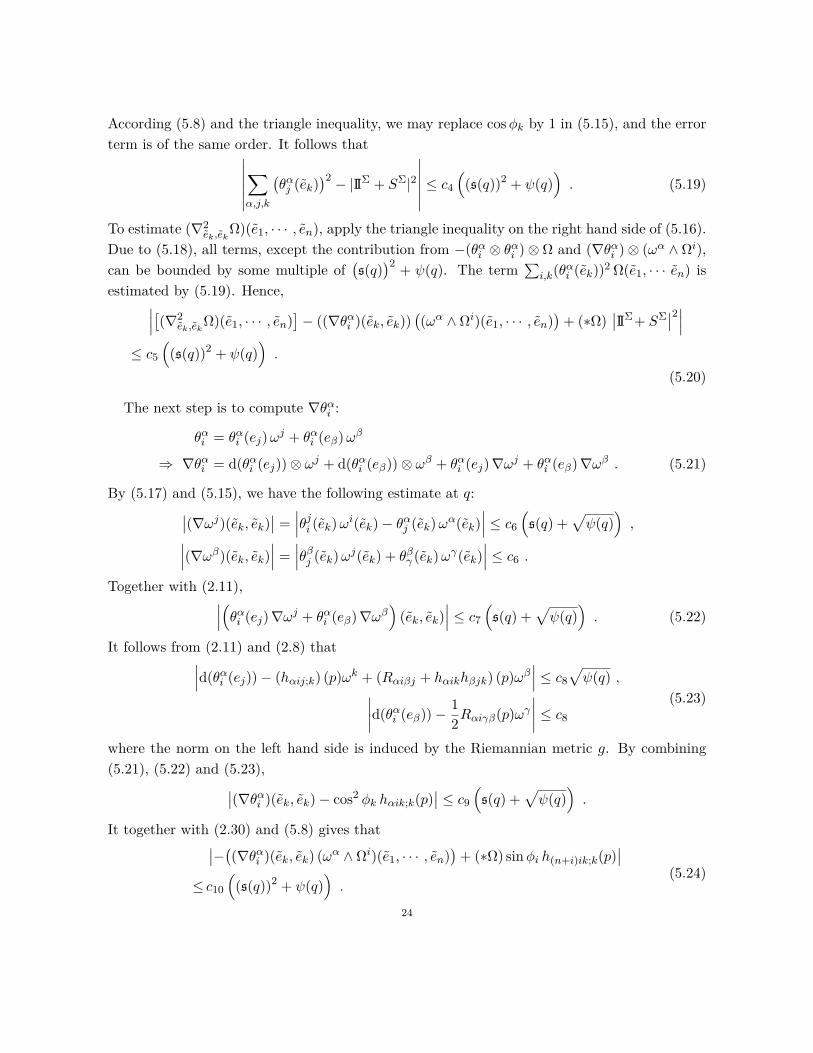
According (5.8) and the triangle inequality, we may replace cosϕk by 1 in (5.15), and the errorterm is of the same order. It follows that∣∣∣∣∣∣

∑α,j,k

(θαj (ek)

)2 − |IIΣ + SΣ|2∣∣∣∣∣∣ ≤ c4

((s(q))2 + ψ(q)

). (5.19)

To estimate (∇2ek,ek

Ω)(e1, · · · , en), apply the triangle inequality on the right hand side of (5.16).Due to (5.18), all terms, except the contribution from −(θαi ⊗ θαi )⊗ Ω and (∇θαi )⊗ (ωα ∧ Ωi),can be bounded by some multiple of

(s(q)

)2+ ψ(q). The term

∑i,k(θ

αi (ek))

2Ω(e1, · · · en) isestimated by (5.19). Hence,∣∣∣[(∇2

ek,ekΩ)(e1, · · · , en)

]− ((∇θαi )(ek, ek))

((ωα ∧ Ωi)(e1, · · · , en)

)+ (∗Ω)

∣∣IIΣ+ SΣ∣∣2∣∣∣

≤ c5((s(q))2 + ψ(q)

).

(5.20)

The next step is to compute ∇θαi :

θαi = θαi (ej)ωj + θαi (eβ)ω

β

⇒ ∇θαi = d(θαi (ej))⊗ ωj + d(θαi (eβ))⊗ ωβ + θαi (ej)∇ωj + θαi (eβ)∇ωβ . (5.21)

By (5.17) and (5.15), we have the following estimate at q:∣∣(∇ωj)(ek, ek)∣∣ = ∣∣∣θji (ek)ωi(ek)− θαj (ek)ωα(ek)

∣∣∣ ≤ c6 (s(q) +√ψ(q)) ,∣∣∣(∇ωβ)(ek, ek)∣∣∣ = ∣∣∣θβj (ek)ωj(ek) + θβγ (ek)ω

γ(ek)∣∣∣ ≤ c6 .

Together with (2.11),∣∣∣(θαi (ej)∇ωj + θαi (eβ)∇ωβ)(ek, ek)

∣∣∣ ≤ c7 (s(q) +√ψ(q)) . (5.22)

It follows from (2.11) and (2.8) that∣∣∣d(θαi (ej))− (hαij;k) (p)ωk + (Rαiβj + hαikhβjk) (p)ω

β∣∣∣ ≤ c8√ψ(q) ,∣∣∣∣d(θαi (eβ))− 1

2Rαiγβ(p)ω

γ

∣∣∣∣ ≤ c8 (5.23)

where the norm on the left hand side is induced by the Riemannian metric g. By combining(5.21), (5.22) and (5.23),∣∣(∇θαi )(ek, ek)− cos2 ϕk hαik;k(p)

∣∣ ≤ c9 (s(q) +√ψ(q)) .

It together with (2.30) and (5.8) gives that∣∣−((∇θαi )(ek, ek) (ωα ∧ Ωi)(e1, · · · , en))+ (∗Ω) sinϕi h(n+i)ik;k(p)

∣∣≤ c10

((s(q))2 + ψ(q)

).

(5.24)

24

It remains to calculate the second term in the asserted inequality of the lemma. By (2.29),∑α,i,k

(−1)iΩ(eα, e1, · · · , ei , · · · , en)Rαkki = (∗Ω)∑i,k

sinϕicosϕi

R(en+i, ek, ek, ei) .

With (2.23), (2.26) and (5.8),∣∣∣∣∣∣∑α,i,k

(−1)iΩ(eα, e1, · · · , ei , · · · , en)Rαkki + (∗Ω)∑i,k

sinϕiR(n+i)kki

∣∣∣∣∣∣ ≤ c11 (s(q))2 .

Since∣∣R(n+i)kki|q −R(n+i)kki|p

∣∣ ≤ c12√ψ(q), we have∣∣∣∣∣∣∑α,i,k

(−1)iΩ(eα, e1, · · · , ei , · · · , en)Rαkki + (∗Ω)∑i,k

sinϕiR(n+i)kki(p)

∣∣∣∣∣∣ ≤ c13((s(q))2 + ψ(q)

).

(5.25)

To conclude the lemma, apply the triangle equality on (5.20), (5.24) and (5.25), and notethat R(n+i)kki(p) = h(n+i)ik;k(p) by (3.5).

Remark 5.3. The tensor SΣ is needed for Lemma 5.2; otherwise the error term would bebigger. However, SΣ will only be used in some intermediate steps in the proof of Theorem B.

5.2.3. The derivative of ∗Ω along Γ. The following lemma relates the derivative of ∗Ω along Γ

and the second fundamental form of Γ.

Lemma 5.4. Let Σn ⊂ (M, g) be a compact, oriented minimal submanifold. Then, there exista positive constant c which depends on the geometry of M and Σ and which has the followingproperty. Suppose that Γ ⊂ Uε is an oriented n-dimensional submanifold with ∗Ω(q) > 1

2 forany q ∈ Γ. Then,

|∇Γ(∗Ω)|2 ≤ c (s(q)(∗Ω))2 |IIΓ − IIΣ|2 + c((s(q))2 + ψ(q)

)2for any q ∈ Γ.

Proof. We compute

∇Γ(∗Ω) = [ej(Ω(e1, · · · , en))] ωj

=

[(∇ejΩ)(e1, · · · , en) +

n∑i=1

Ω(e1, · · · , ei−1,∇ej ei, ei+1, · · · , en)

]ωj

=

[(∇ejΩ)(e1, · · · , en) +

n∑i=1

hαijΩ(e1, · · · , ei−1, eα, ei+1, · · · , en)

]ωj .

Note that the expression is tensorial, and we use the frame (2.23) and (2.26) to proceed.25

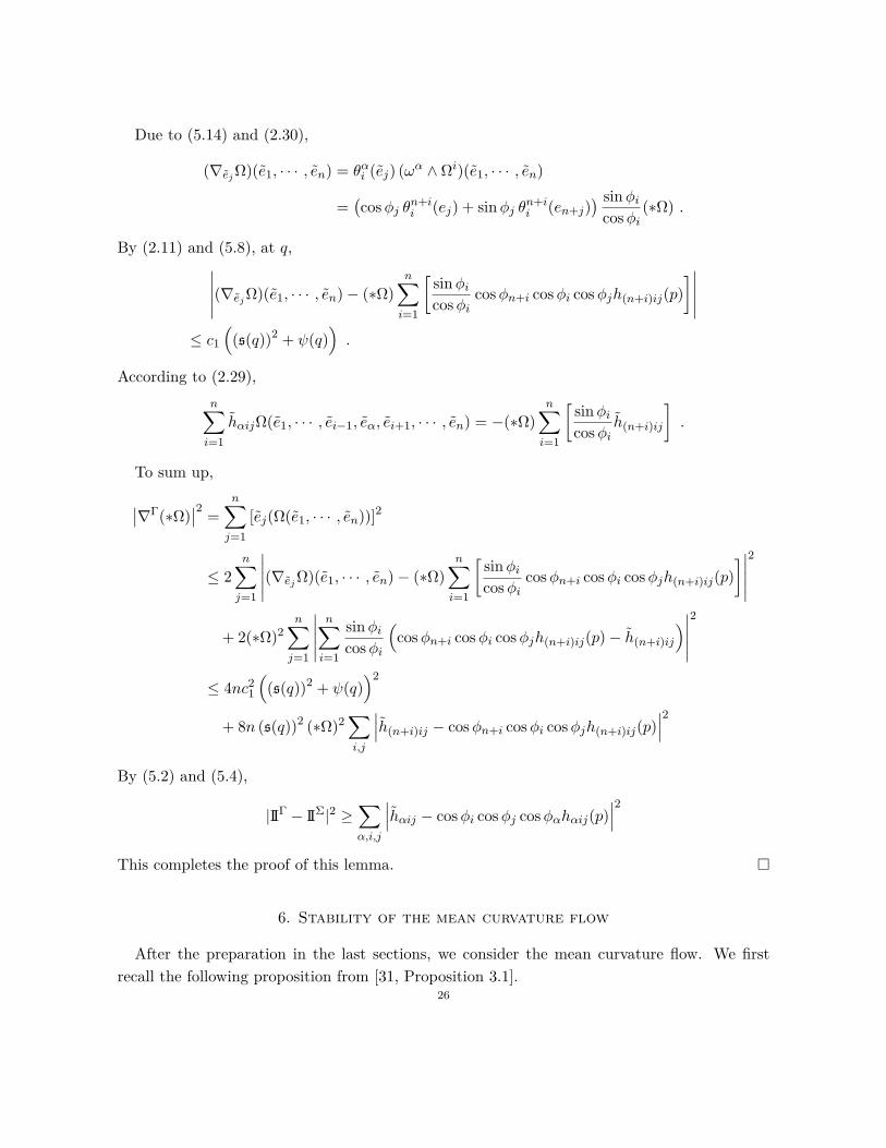
Due to (5.14) and (2.30),

(∇ejΩ)(e1, · · · , en) = θαi (ej) (ωα ∧ Ωi)(e1, · · · , en)

=(cosϕj θ

n+ii (ej) + sinϕj θ

n+ii (en+j)

) sinϕicosϕi

(∗Ω) .

By (2.11) and (5.8), at q,∣∣∣∣∣(∇ejΩ)(e1, · · · , en)− (∗Ω)n∑

i=1

[sinϕicosϕi

cosϕn+i cosϕi cosϕjh(n+i)ij(p)

]∣∣∣∣∣≤ c1

((s(q))2 + ψ(q)

).

According to (2.29),n∑

i=1

hαijΩ(e1, · · · , ei−1, eα, ei+1, · · · , en) = −(∗Ω)n∑

i=1

[sinϕicosϕi

h(n+i)ij

].

To sum up,

∣∣∇Γ(∗Ω)∣∣2 = n∑

j=1

[ej(Ω(e1, · · · , en))]2

≤ 2n∑

j=1

∣∣∣∣∣(∇ejΩ)(e1, · · · , en)− (∗Ω)n∑

i=1

[sinϕicosϕi

cosϕn+i cosϕi cosϕjh(n+i)ij(p)

]∣∣∣∣∣2

+ 2(∗Ω)2n∑

j=1

∣∣∣∣∣n∑

i=1

sinϕicosϕi

(cosϕn+i cosϕi cosϕjh(n+i)ij(p)− h(n+i)ij

)∣∣∣∣∣2

≤ 4nc21

((s(q))2 + ψ(q)

)2+ 8n (s(q))2 (∗Ω)2

∑i,j

∣∣∣h(n+i)ij − cosϕn+i cosϕi cosϕjh(n+i)ij(p)∣∣∣2

By (5.2) and (5.4),

|IIΓ − IIΣ|2 ≥∑α,i,j

∣∣∣hαij − cosϕi cosϕj cosϕαhαij(p)∣∣∣2

This completes the proof of this lemma.

6. Stability of the mean curvature flow

After the preparation in the last sections, we consider the mean curvature flow. We firstrecall the following proposition from [31, Proposition 3.1].

26

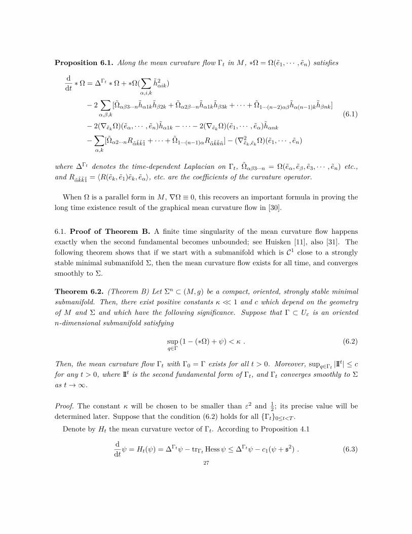
Proposition 6.1. Along the mean curvature flow Γt in M , ∗Ω = Ω(e1, · · · , en) satisfies

d

dt∗ Ω = ∆Γt ∗ Ω+ ∗Ω(

∑α,i,k

h2αik)

− 2∑α,β,k

[Ωαβ3···nhα1khβ2k + Ωα2β···nhα1khβ3k + · · ·+ Ω1···(n−2)αβhα(n−1)khβnk]

− 2(∇ekΩ)(eα, · · · , en)hα1k − · · · − 2(∇ekΩ)(e1, · · · , eα)hαnk

−∑α,k

[Ωα2···nRαkk1 + · · ·+ Ω1···(n−1)αRαkkn]− (∇2ek,ek

Ω)(e1, · · · , en)

(6.1)

where ∆Γt denotes the time-dependent Laplacian on Γt, Ωαβ3···n = Ω(eα, eβ, e3, · · · , en) etc.,and Rαkk1 = ⟨R(ek, e1)ek, eα⟩, etc. are the coefficients of the curvature operator.

When Ω is a parallel form in M , ∇Ω ≡ 0, this recovers an important formula in proving thelong time existence result of the graphical mean curvature flow in [30].

6.1. Proof of Theorem B. A finite time singularity of the mean curvature flow happensexactly when the second fundamental becomes unbounded; see Huisken [11], also [31]. Thefollowing theorem shows that if we start with a submanifold which is C1 close to a stronglystable minimal submanifold Σ, then the mean curvature flow exists for all time, and convergessmoothly to Σ.

Theorem 6.2. (Theorem B) Let Σn ⊂ (M, g) be a compact, oriented, strongly stable minimalsubmanifold. Then, there exist positive constants κ << 1 and c which depend on the geometryof M and Σ and which have the following significance. Suppose that Γ ⊂ Uε is an orientedn-dimensional submanifold satisfying

supq∈Γ

(1− (∗Ω) + ψ) < κ . (6.2)

Then, the mean curvature flow Γt with Γ0 = Γ exists for all t > 0. Moreover, supq∈Γt|IIt| ≤ c

for any t > 0, where IIt is the second fundamental form of Γt, and Γt converges smoothly to Σ

as t→∞.

Proof. The constant κ will be chosen to be smaller than ε2 and 12 ; its precise value will be

determined later. Suppose that the condition (6.2) holds for all Γt0≤t<T .Denote by Ht the mean curvature vector of Γt. According to Proposition 4.1

d

dtψ = Ht(ψ) = ∆Γtψ − trΓt Hessψ ≤ ∆Γtψ − c1(ψ + s2) . (6.3)

27

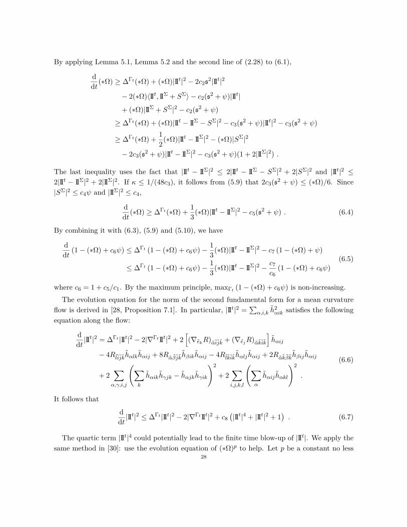
By applying Lemma 5.1, Lemma 5.2 and the second line of (2.28) to (6.1),

d

dt(∗Ω) ≥ ∆Γt(∗Ω) + (∗Ω)|IIt|2 − 2c2s

2|IIt|2

− 2(∗Ω)⟨IIt, IIΣ + SΣ⟩ − c2(s2 + ψ)|IIt|

+ (∗Ω)|IIΣ + SΣ|2 − c2(s2 + ψ)

≥ ∆Γt(∗Ω) + (∗Ω)|IIt − IIΣ − SΣ|2 − c3(s2 + ψ)|IIt|2 − c3(s2 + ψ)

≥ ∆Γt(∗Ω) + 1

2(∗Ω)|IIt − IIΣ|2 − (∗Ω)|SΣ|2

− 2c3(s2 + ψ)|IIt − IIΣ|2 − c3(s2 + ψ)(1 + 2|IIΣ|2) .

The last inequality uses the fact that |IIt − IIΣ|2 ≤ 2|IIt − IIΣ − SΣ|2 + 2|SΣ|2 and |IIt|2 ≤2|IIt − IIΣ|2 + 2|IIΣ|2. If κ ≤ 1/(48c3), it follows from (5.9) that 2c3(s

2 + ψ) ≤ (∗Ω)/6. Since|SΣ|2 ≤ c4ψ and |IIΣ|2 ≤ c4,

d

dt(∗Ω) ≥ ∆Γt(∗Ω) + 1

3(∗Ω)|IIt − IIΣ|2 − c5(s2 + ψ) . (6.4)

By combining it with (6.3), (5.9) and (5.10), we have

d

dt(1− (∗Ω) + c6ψ) ≤ ∆Γt (1− (∗Ω) + c6ψ)−

1

3(∗Ω)|IIt − IIΣ|2 − c7 (1− (∗Ω) + ψ)

≤ ∆Γt (1− (∗Ω) + c6ψ)−1

3(∗Ω)|IIt − IIΣ|2 − c7

c6(1− (∗Ω) + c6ψ)

(6.5)

where c6 = 1 + c5/c1. By the maximum principle, maxΓt (1− (∗Ω) + c6ψ) is non-increasing.The evolution equation for the norm of the second fundamental form for a mean curvature

flow is derived in [28, Proposition 7.1]. In particular, |IIt|2 =∑

α,i,k h2αik satisfies the following

equation along the flow:

d

dt|IIt|2 = ∆Γt |IIt|2 − 2|∇ΓtIIt|2 + 2

[(∇ekR)αijk + (∇ejR)αkik

]hαij

− 4Rlijkhαlkhαij + 8Rαβjkhβikhαij − 4Rlkikhαlj hαij + 2Rαkβkhβij hαij

+ 2∑

α,γ,i,j

(∑k

hαikhγjk − hαjkhγik

)2

+ 2∑i,j,k,l

(∑α

hαij hαkl

)2

.

(6.6)

It follows that

d

dt|IIt|2 ≤ ∆Γt |IIt|2 − 2|∇ΓtIIt|2 + c8

(|IIt|4 + |IIt|2 + 1

). (6.7)

The quartic term |IIt|4 could potentially lead to the finite time blow-up of |IIt|. We apply thesame method in [30]: use the evolution equation of (∗Ω)p to help. Let p be a constant no less

28

than 1, whose precise value will be determined later. According to (6.4),d

dt(∗Ω)p = p(∗Ω)p−1 d

dt(∗Ω)

≥ p(∗Ω)p−1∆Γt(∗Ω) + p

3(∗Ω)p|IIt − IIΣ|2 − c5p(s2 + ψ)

= ∆Γt(∗Ω)p − p(p− 1)(∗Ω)p−2|∇Γt(∗Ω)|2 + p

3(∗Ω)p|IIt − IIΣ|2 − c5p(s2 + ψ) .

After an appeal to Lemma 5.4,d

dt(∗Ω)p ≥ ∆Γt(∗Ω)p + p

3

(1− c9 p s2

)(∗Ω)p|IIt − IIΣ|2 − c9 p2(s2 + ψ) .

If κ ≤ 1/(24c9p), it follows from (5.9) that c9 p s2 ≤ 1/12. It together with (6.3) gives thatd

dt

((∗Ω)p −Kp2ψ

)≥ ∆Γt

((∗Ω)p −Kp2ψ

)+p

4

((∗Ω)p −Kp2ψ

)|IIt − IIΣ|2 (6.8)

where K = c9/c1. The maximum principle implies that if (∗Ω)p − Kp2ψ > 0 on Γ, thenminΓt

((∗Ω)p −Kp2ψ

)is non-decreasing. Moreover, for any p ≥ 1, we may choose κ such that

(6.2) implies that (∗Ω)p −Kp2ψ > 1/2 on Γ.Denote (∗Ω)p −Kp2ψ by η. Due to (6.7) and (6.8),

d

dt(η−1|IIt|2) ≤ η−1∆Γt |IIt|2 − 2η−1|∇ΓtIIt|2 + c8η

−1(|IIt|4 + |IIt|2 + 1

)− η−2|IIt|2

(∆Γtη +

p

4η|IIt − IIΣ|2

).

Since

∆Γt(η−1|IIt|2) = η−1∆Γt |IIt|2 + |IIt|2∆Γtη−1 + 2⟨∇Γtη−1,∇Γt |IIt|2⟩

= η−1∆Γt |IIt|2 − η−2|IIt|2∆Γtη + 2η−3|∇Γtη|2|IIt|2 − 2η−2⟨∇Γtη,∇Γt |IIt|2⟩

= η−1∆Γt |IIt|2 − η−2|IIt|2∆Γtη − 2η−1⟨∇Γtη,∇Γt(η−1|IIt|2)⟩

and |IIt − IIΣ|2 ≥ 12 |II

t|2 − c10, we haved

dt(η−1|IIt|2) ≤ ∆Γt(η−1|IIt|2) + 2η−1⟨∇Γtη,∇Γt(η−1|IIt|2)⟩

− p

8η−1|IIt|4 + c10

p

4η−1|IIt|2 + c8η

−1(|IIt|4 + |IIt|2 + 1

)≤ ∆Γt(η−1|IIt|2) + 2η−1⟨∇Γtη,∇Γt(η−1|IIt|2)⟩

− 1

2

(p8− c8

)(η−1|IIt|2)2 +

(c8 + c10

p

4

)(η−1|IIt|2) + 2c8

(6.9)

(provided that p ≥ 8c8). Choose p > 8c8. It follows from the maximum principle that η−1|IIt|2

is uniformly bounded, and hence there is no finite time singularity.

The C0 convergence is easy to come by. The differential inequality (6.3) implies that ψconverges to zero exponentially. Similarly, it follows from (6.5) that 1 − (∗Ω) + c6ψ converges

29

to zero exponentially. Therefore, ∗Ω converges to 1 exponentially, and we conclude the C1

convergence.

For the C2 and smooth convergence, consider η = (∗Ω)p −Kp2ψ. It follows from the abovediscussion that η has a positive lower bound. It is clear that η ≤ 1. Moreover, η converges to1 as t→∞. Integrating (6.8) gives∫

Γt

|IIt − IIΣ|2 dµt ≤ c12∫Γt

dη

dtdµt .

Recall that the Lie derivative of dµt in Ht is −|H2t |dµt; see [28, §2]. It follows that

1

c12

∫Γt

|IIt − IIΣ|2 dµt ≤d

dt

∫Γt

η dµt +

∫Γt

η |Ht|2 dµt (6.10)

We claim that the improper integral of the right hand side for 0 ≤ t < ∞ converges. Tostart, note that d

dt

∫Γt

dµt = −∫Γt|Ht|2 dµt ≤ 0. Thus, vol(Γt) =

∫Γt

dµt is positive and non-increasing, and must converge as t→∞. For the first term on right hand side of (6.10),∫ t

0

(d

ds

∫Γs

η dµs

)ds =

∫Γt

η dµt −∫Γ0

η dµ0

Since η converges to 1 (uniformly) and vol(Γt) converges as t → ∞,∫Γtη dµt converges as

t→∞. For the second term on the right hand side of (6.10),∫ t

0

(∫Γs

η |Hs|2 dµs)ds ≤

∫ t

0

(∫Γs

|Hs|2 dµs)ds =

∫ t

0

(− d

ds

∫Γs

dµs

)ds

= vol(Γ0)− vol(Γt) ≤ vol(Γ0) .

It is bounded from above, and is clearly non-decreasing in t. Therefore, it converges as t→∞.It follows from the claim and (6.10) that∫ ∞

0

(∫Γt

|IIt − IIΣ|2 dµt)dt <∞ . (6.11)

On the other hand, |IIt − IIΣ|2 obeys a differential inequality of the same form as (6.7):d

dt|IIt − IIΣ|2 ≤ ∆Γt |IIt − IIΣ|2 + c13

(|IIt − IIΣ|4 + |IIt − IIΣ|2 + 1

). (6.12)

The derivation for this inequality is in Appendix B. By (6.12) and the uniform boundedness of|IIt|, d

dt

∫Γt|IIt− IIΣ|2 dµt is bounded from above uniformly. Due to Lemma 6.3, which is proved

at the end of this subsection, we find that

limt→0

∫Γt

|IIt − IIΣ|2 dµt = 0 . (6.13)

Since we have shown long time existence and convergence in C1, for t large enough Γt canbe written as a graph (in the geodesic coordinate defined in §2.2) over Σ defined by yα =

30

fαt , α = n + 1, · · ·n + m for C1 functions fαt on Σ. With (6.13), a Moser iteration argumentsimilar to [12, §5] shows that fαt converges to 0 in C2. The detail of this argument is includedin Appendix C. With the C2 convergence, standard arguments for a second order quasilinearparabolic system lead to the smooth convergence of fαt .

Lemma 6.3. Let a > 0 and f(t) be a smooth function for t ∈ (a,∞). Suppose that f(t) ≥ 0,∫∞a f(t) dt converges, and f ′(t) ≤ C for some constant C > 0. Then, f(t)→ 0 as t→∞.

Proof. It follows from f ′(t) ≤ C that f(t) ≥ f(t1)−C(t1− t) for any t1 > t > a. Since f(t) ≥ 0

and∫∞a f(t) dt < ∞, given any ϵ ∈ (0, 1), there exists an Aϵ > a such that

∫∞Aϵf(t) dt < ϵ.

Thus, for any t1 > Aϵ + 1 > Aϵ +√ϵ,

ϵ >

∫ t1

t1−√ϵf(t) dt ≥

∫ t1

t1−√ϵ(f(t1)− C(t1 − t)) dt

=√ϵ (f(t1)− C t1) + C

(√ϵ t1 −

1

2ϵ

).

It follows that f(t) < (1 + 12C)√ϵ for any t > Aϵ + 1.

6.2. With only the stability condition. Theorem 6.2 asserts that a strongly stable minimalsubmanifold is C1 dynanical stable under the mean curvature flow. Recall that a minimalsubmanifold is said to be stable if the Jacobi operator, (∇⊥)∗∇⊥+R−A, is a positive operator.It is a natural question whether the stability condition already implies the dynamical stability.This was investigated by Naito in [18]. The answer is yes, but initial submanifold has to beclose to the stable one in a higher norm.

The approach of Naito is to consider only graphical/sectional type submanifold, i.e. Γt isgiven by a section s of the normal bundle of Σ. Then, the mean curvature flow equation takesthe following form

∂s

∂t= −

((∇⊥)∗∇⊥ +R−A

)(s) +N (s) (6.14)

where N is a “small” operator in the sense of [18, (C3) on p.222]. The positivity of the Jacobioperator takes over the behavior of the parabolic system if one works with a suitable norm. Inthe mean curvature flow case, [18, Theorem 5.3] reads as follows.

Theorem 6.4. Let Σn ⊂ (M, g) be a compact, oriented, stable minimal submanifold. Then,for any r > n

2 + 2, there exists a positive constant κ′ << 1 such that for any section s0 of NΣ

with ||s0||Hr ≤ κ′, the mean curvature flow (6.14) exists for any t > 0. Moreover, the solutionconverges to 0 exponentially as t→∞ in Hr norm.

According to the Sobolev embedding theorem, Hr → C⌊r−n2⌋,α where α = r − n

2 − ⌊r −n2 ⌋ ∈

(0, 1]. In other words, the assumption implies that s0 has small C2,α norm.31

Remark 6.5. The initial condition in [18, Proposition 5.2 and Theorem 5.3] looks more com-plicated than above stated. See [18, p.223–224] for the norm. The reason is that Naito alsodiscussed the case when the Jacobi operator has non-positive spectrum. If the Jacobi operatoris positive, one can check directly by using the spectral decomposition that the norm conditionthere is equivalent to the Hr norm (r here corresponds to m in [18]).

In the rest of this subsection, we will briefly explain how to set up (6.14) and check thecondition [18, (C3)]. Although this was demonstrated in [18, p.233–235] under a general setting,it is instructive to do it for the mean curvature flow case.

6.2.1. The expansion in radial direction. To highlighting the computation for a section of NΣ,we build the expansion of the metric coefficients in the radial directions. Let xi be an oriented,local coordinate system of Σ. Choose a local orthonormal frame eµ for NΣ. As in section2.2, construct a local coordinate of M by(

(x1, · · · , xn), (yn+1, · · · , yn+m))7→ exp(x1,··· ,xn)(y

βeβ) .

Here, xi needs not to be the Gaussian coordinate for Σ. Denote by gAB(x,y) the coefficientsof the Riemannian metric g in this coordinate system.

Denote the normal bundle connection by Aνµ, i.e. ∇⊥eµ = (Aν

µ i dxi) eν . By the Jacobi field

argument similar to that in section 2.2,gij(x,y) = gij − 2yβhβij − yµyν(Rjµiν − hµikhνjℓgkℓ −Aβ

µ iAβν j) +O(|y|3) ,

giµ(x,y) = yνAµν i +O(|y|2) ,

gµν(x,y) = δµν +O(|y|2)

(6.15)

where all the coefficient functions on the right hand side are evaluated at (x, 0) ∈ Σ.For a section Γ = yµ = yµ(x), the ij component of the induced metric is

gij = gij(x,y) + giµ(x,y) ∂jyµ + gjµ(x,y) ∂iy

µ + gµν(x,y)(∂iyµ)(∂jy

ν)

= gij − 2yβhβij − yµyν(Rjµiν − hµikhνjℓgkℓ) + yµ;iyµ;j

+O(|y|3) +O(|y|2)(∂y) +O(|y|2)(∂y)2(6.16)

where yµ;i = ∂iyµ +Aµ

ν iyν . We will also need

gµν =

⟨(∂

∂yµ

)⊥,

(∂

∂yν

)⊥⟩

= gµν − gij(gµj + gµα∂jyα)(gνi + gνβ∂iy

β) (6.17)

where ⊥ is the orthogonal projection onto NΓ.It is convenient to think ∂jyν as a dummy variable pνj , and regard them as the same order as

yµ. The negative gradient flow of vol(Γ) =∫ √

det g dx1∧· · ·∧dxn is almost the mean curvature32

flow. Recall that

det(I + T ) = 1 + tr(T ) +1

2(tr2(T )− tr(T 2)) +O(|T |3)

for T small. With gijhβij = 0,det g

det g= 1 + gij

[yµ;iy

µ;j − y

µyν(Rjµiν − hµikhνjℓgkℓ)]+

1

2(2yµhµikg

kℓ)(2yνhνℓjgji) +O(3)

= 1 + gij[yµ;iy

µ;j − y

µyν(Rjµiν + hµikhνjℓgkℓ)]+O(3) .

The notation O(3) means O((|y|2 + |p|2) 32 ) for y, p small; see also (C.1) for the definition of

this notation. Hence,√det g =

√det g +

√det g

2gij[yµ;iy

µ;j − y

µyν(Rjµiν + hµikhνjℓgkℓ)]+ E(x,y,p) (6.18)

where E = O(3). Since the computation is based on the graphical setting, the mean curvatureflow equation shall be (∂ty)

⊥ = HΓt . With some linear algebraic computations, the meancurvature flow equation reads

∂yµ

∂t=

gµν√det g

[d

dxk

(∂√det g

∂pνk

)− ∂√det g

∂yν

]. (6.19)

According to (6.15), (6.16), (6.17) and (6.18), gµν = δµν +O(2).The zero-th order term of (6.18) gives the volume of the zero section, and has no contribution

in the Euler–Lagrange equation. The integral of the quadratic term of (6.18) is1

2

∫Σ

(|∇⊥y|2 + ⟨R(y),y⟩ − ⟨A(y),y⟩

)dvolΣ .

Therefore, its Euler–Lagrange operator is the Jacobi operator (∇⊥)∗∇⊥+R−A at y = 0, withrespect to the volume form dvolΣ. It follows that the contribution of the quadratic terms of(6.18) to the right hand side of (6.19) is

gµν

√det g

det g

(−[(∇⊥)∗∇⊥ +R−A]y

)µ=(−[(∇⊥)∗∇⊥ +R−A]y

)µ+ Eµν (x,y,p)

(−[(∇⊥)∗∇⊥ +R−A]y

)νwhere Eµν = O(2).

To sum up, the mean curvature flow equation takes the following form∂yµ

∂t=(−[(∇⊥)∗∇⊥ +R−A]y

)µ+ Eµν ·

(−[(∇⊥)∗∇⊥ +R−A]y

)ν+

gµν√det g

[d

dxk

(∂E∂pνk

)− ∂E∂yν

].

The operator in the last line in the remainder operator N ; see (6.14).33

6.2.2. The smallness of the remainder operator. The condition [18, (C3)] says that for anyr > n

2 + 2 there exists a constant C > 0 such that

||N (y)−N (y)||Hr−1 ≤ C (||y||Hr ||y − y||Hr+1 + ||y − y||Hr ||y||Hr+1) (C3)

for any two sections y, y ∈ L2r+1 with ||y||Hr+1 < 1, ||y||Hr+1 < 1.

There are some different types of terms in N . What follows is a brief explanation for termslike f(x,y, ∂y)(∂y)(∂2y). Write

f(x,y, ∂y)(∂y)(∂2y)− f(x, y, ∂y)(∂y)(∂2y)

= f(x,y, ∂y)(∂y)[(∂2y)− (∂2y)

]+ [h1(x,y, y, ∂y, ∂y) (y − y) + h2(x,y, y, ∂y, ∂y) (∂y − ∂y)] (∂2y)

where h1 and h2 are constructed from the derivatives of f(x,y, ∂y)(∂y) in y and in ∂y, respec-tively. With the following two bullets, f(x,y, ∂y)(∂y)(∂2y) does obey the condition (C3).

• According to [20, Lemma 9.9], the “coefficients” f(x,y, ∂y), h1(x,y, y, ∂y, ∂y) andh1(x,y, y, ∂y, ∂y) have bounded Hr norm.• Due to [20, Theorem 9.5 and Corollary 9.7], for any r−1 > n

2 , there exists C ′ > 0 suchthat

||uv||Hr−1 ≤ C ′ ||u||Hr−1 ||v||Hr−1

for any u,v ∈ Hr−1.

For other types of terms, the argument is similar.

Appendix A. Computations related to strong stability

For minimal Lagrangians in a Kähler–Einstein manifold and coassociatives in a G2 manifold,the condition (3.2) can be rewritten as a curvature condition on the submanifold. One ingredientis the geometric properties of U(n) and G2 holonomy. Another ingredient is the Gauss equation:

Rijkℓ −RΣijkℓ = hαiℓhαjk − hαikhαjℓ . (A.1)

A.1. Minimal Lagrangians in Kähler–Einstein manifolds. Let (M2n, g, J, ω) be a Kähler–Einstein manifold, where J is the complex structure and ω is the Kähler form. Denote theEinstein constant by c; namely, ∑

C

RACBC = RicAB = c gAB .

A submanifold Ln ⊂ M2n is Lagrangian if ω|L vanishes. It implies that J induces an iso-morphism between its tangent bundle TL and normal bundle NL. In terms of the notations

34

introduced in §2.1, the correspondence is

viei ←→ vi Jei . (A.2)

In particular, if e1, · · · , en is an orthonormal frame for TL, Je1, · · · , Jen is an orthonor-mal frame for NL. Denote Jek by eJ(k), and let

Ckij = hJ(k)ij = ⟨∇eiej , Jek⟩ .

Since J is parallel, it is easy to verify that Ckij is totally symmetric.Now, suppose that L is also minimal. By using the correspondence (A.2), the strong stability

condition (3.2) can be rewritten as follows.

−RiJ(k)iJ(ℓ) vk vℓ − Ckij Cℓij v

k vℓ = −c gkℓ vk vℓ +RJ(i)J(k)J(i)J(ℓ) vk vℓ − Ckij Cℓij v

k vℓ

= −c |v|2 +Rikiℓ vk vℓ − Ckij Cℓij v

k vℓ

= −c |v|2 +RLikiℓ v

k vℓ + CjkiCjℓi vk vℓ − Ckij Cℓij v

k vℓ

= −c |v|2 +RicL(v, v) .

The first equality uses the Kähler–Einstein condition. The second equality follows from theparallelity of J . The third equality uses the Gauss equation and the minimal condition. Thelast equality relies on the fact that Ckij is totally symmetric. This computation says that (3.2)is equivalent to the condition that RicL − c is a positive definite operator on TL.

A.2. Coassociative submanifolds in G2 manifolds. In this case, the ambient space is 7-dimensional, and the submanifold is 4-dimensional.

A.2.1. Four dimensional Riemannian geometry. The Riemann curvature tensor has a nice de-composition in 4 dimensions. What follows is a brief summary of the decomposition; readersare directed to [1] for more.

Let Σ be an oriented, 4-dimensional Riemannian manifold. The Riemann curvature tensorin general defines a self-adjoint transform on Λ2 by

R(ei ∧ ej) =1

2RΣ

kℓij ek ∧ eℓ .

In 4 dimensions, Λ2 decomposes into self-dual, Λ2+, and anti-self-dual part, Λ2

−. In terms of thedecomposition Λ2 = Λ2

+ ⊕ Λ2−, the curvature map R has the form

R =

[W+ + s

12 I B

BT W− + s12 I

].

Here, s = RΣijij is the scalar curvature, W± is the self-dual and anti-self-dual part of the Weyl

tensor, B is the traceless Ricci tensor, and I is the identity homomorphism.35

With respect to the basis e1 ∧ e2− e3 ∧ e4, e1 ∧ e3+ e2 ∧ e4, e1 ∧ e4− e2 ∧ e3, the lower-rightblock W− + s

12 I is

1

2

RΣ

1212 +RΣ3434 − 2RΣ

1234 RΣ1213 +RΣ

1224 −RΣ3413 −RΣ

3424 RΣ1214 −RΣ

1223 −RΣ3414 +RΣ

3423

RΣ1312 −RΣ

1334 +RΣ2412 −RΣ

2434 RΣ1313 +RΣ

2424 + 2RΣ1324 RΣ

1314 −RΣ1323 +RΣ

2414 −RΣ2423

RΣ1412 −RΣ

1434 −RΣ2312 +RΣ

2334 RΣ1413 +RΣ

1424 −RΣ2313 −RΣ

2324 RΣ1414 +RΣ

2323 − 2RΣ1423

.(A.3)

The operator will be needed is W−− s6 I = (W−+ s

12 I)−s4 I. One-fourth of the scalar curvature

is

s

4=

1

2

(RΣ

1212 +RΣ3434 +RΣ

1313 +RΣ2424 +RΣ

1313 +RΣ2424

). (A.4)

A.2.2. G2 geometry. A 7-dimensional Riemannian manifold M whose holonomy is containedin G2 can be characterized by the existence of a parallel, positive 3-form φ. A complete storycan be found in [13, ch.11]. In terms of a local orthonormal coframe, the 3-form and its Hodgestar are

φ = ω567 + ω125 − ω345 + ω136 + ω246 + ω147 − ω237 ,

∗φ = ω1234 − ω1267 + ω3467 + ω1357 + ω3457 − ω1456 + ω2356(A.5)

where ω123 is short for ω1∧ω2∧ω3. It is known that the holonomy is G2 if and only if ∇φ = 0,which is also equivalent to dφ = 0 = d ∗ φ.

Remark A.1. There are two commonly used conventions for the 3-form; see [14] for instance.The convention here is the same as that in [16]; the deformation of coassociatives will then bedetermined by anti-self-dual harmonic forms. If one use the convention in [13], the deformationof coassociatives will be determined by self-dual harmonic forms.

The 3-form φ determines a product map × for tangent vectors of M . For any two tangentvectors X and Y ,

X × Y =(φ(X,Y, · )

)♯.

For instance, e1×e2 = e5. Since φ and the metric tensor are both parallel, × is parallel as well.As a consequence,

R(eA, eB)(e1 × e2) =(R(eA, eB)e1

)× e2 + e1 ×

(R(eA, eB)e2

),

36

and its e3-component gives R53AB − R62AB − R71AB = 0 for any A,B ∈ 1, . . . , 7. In total,the parallelity of × leads to following seven identities:

R52AB +R63AB +R74AB = 0 ,

R51AB −R64AB +R73AB = 0 ,

R54AB +R61AB −R72AB = 0 ,

−R53AB +R62AB +R71AB = 0 ,

R67AB +R12AB −R34AB = 0 ,

−R57AB +R13AB +R24AB = 0 ,

R56AB −R14AB −R23AB = 0 .

(A.6)

These identities imply that a G2 manifold is always Ricci flat.

A.2.3. Coassociative geometry. According to [10, §IV], an oriented, 4-dimensional submanifoldΣ of a G2 manifold is said to be coassociative if ∗φ|Σ coincides with the volume form of theinduced metric. Harvey and Lawson also proved that if φ|Σ vanishes, there is an orientationon Σ so that it is coassociative. Similar to the Lagrangian case, the normal bundle of a coasso-ciative submanifold is canonically isomorphic to an intrinsic bundle. The following discussionis basically borrowed from [16, §4].

Orthonormal frame. Suppose that Σ ⊂M is coassociative. One can find a local orthonormalframe e1, · · · , e7 such that e1, e2, e3, e4 are tangent to Σ, e5, e6, e7 are normal to Σ, andφ takes the form (A.5) in this frame. Here is a sketch of the construction. Start with a unitnormal vector, e5, and a unit tangent vector, e1, of Σ. Let e2 = e5 × e1. Then, set e3 to be aunit vector tangent to Σ and orthogonal to e1, e2. Finally, let e4 = e3 × e5, e6 = e1 × e3 ande7 = e3 × e2.

Normal bundle and second fundamental form. The normal bundle of Σ is isomorphic to thebundle of anti-self-dual 2-forms of Σ via the following map:

V 7→ (V yφ)|Σ . (A.7)

In terms of the above frame, e5 corresponds to ω12 − ω34, e6 corresponds to ω13 + ω24, and e7

corresponds to ω14 − ω23.As shown in [10], a coassociative submanifold must be minimal. In fact, its second funda-

mental form has certain symmetry. For instance,

h51i = ⟨∇eie1, e5⟩ = −⟨e1,∇ei(e6 × e7)⟩

= −⟨e1, (∇eie6)× e7⟩ − ⟨e1, e6 × (∇eie7)⟩

= −⟨e4,∇eie6⟩+ ⟨e3,∇eie7⟩ = h64i − h73i .

What follows are all the relations:h52i + h63i + h74i = 0 ,

h51i − h64i + h73i = 0 ,

h54i + h61i − h72i = 0 ,

−h53i + h62i + h71i = 0(A.8)

37

for any i ∈ 1, 2, 3, 4. These relations imply that the mean curvature vanishes. They can beencapsulated as

∑j ej × II(ei, ej) = 0.

A.2.4. Strong stability for coassociatives. For any sections of NΣ, v, denote the symmetricbilinear form on the left hand side of (3.2) by Q(v,v). Under the identification (A.7), Q(v,v) =

−2vT W− v + s3 |v|

2 is also a symmetric bilinear form.We now check that Q(v,v) = Q(v,v) for any unit vector v ∈ NpΣ at any p ∈ Σ. As explained

above, we may take e5 = v and construct the other orthonormal vectors. With respect such aframe, it follows from (A.3) and (A.4) that

Q(v,v) = RΣ1313 +RΣ

2424 +RΣ1313 +RΣ

2424 + 2RΣ1234 .

The quantity Q(v,v) can be rewritten as follows.

Q(v,v) = −∑i

Ri5i5 −∑i,j

(h5ij)2

= R6565 +R7575 −∑i,j

(h5ij)2

= R1313 +R2424 +R1313 +R2424 − 2R1423 + 2R1324 −∑i,j

(h5ij)2

= R1313 +R2424 +R1313 +R2424 + 2R1234 −∑i,j

(h5ij)2 .

The second equality follows from Ricci flatness. The third equality uses (A.6). The last equalityis the first Bianchi identity. With the Gauss equation and some simple manipulation,

Q(v,v)− Q(v,v)

=∑α

((hα14 + hα23)

2 + (hα13 − hα24)2 − (hα11 + hα22)(hα33 + hα44))−∑i,j

(h5ij)2 . (A.9)

By appealing to (A.8),

h614 + h623 = −h522 − h544 = h511 + h533 ,

h714 + h723 = −h512 + h534 ,

h613 − h624 = −h512 − h534 ,

h713 − h724 = −h522 + h533 = −h511 − h544 ,

and

h611 + h622 = −h633 − h644 = −h514 + h523 ,

h711 + h722 = −h733 − h744 = h513 + h524 .

By using these relations, it is not hard to verify that (A.9) vanishes. Therefore, the strongstability condition (3.2) is equivalent to the positivity of −2W− + s

3 .38

As a final remark, this equivalence can also be seen by combining [16, Theorem 4.9] and theWeitzenböck formula [9, Appendix C]. Nevertheless it is nice to derive the equivalence directlyby highlighting the geometry of G2.

Appendix B. Evolution equation for tensors

Suppose that Ψ be a tensor defined on M of type (0, 3). The main purpose of this sectionis to calculate its evolution equation along the mean curvature flow. Since there will be somedifferent connections, we denote the Levi-Civita connection of (M, g) by ∇ to avoid confusions.

Let Γt be the mean curvature flow at time t. The tensor Ψ is a section of (T ∗M ⊗ T ∗M ⊗T ∗M)|Γt . The connection ∇ naturally induces a connection ∇ on this bundle. The onlydifference between ∇ and ∇ is that the direction vector in ∇ must be tangent to Γt.

connection bundle and base∇ Levi-Civita connection of (M, g)

∇Γt Levi-Civita connection of Γt with the induced metric∇⊥ connection of the normal bundle of Γt

∇ connection of (T ∗M ⊗ T ∗M ⊗ T ∗M)|Γt

∇ connection of T ∗Γt ⊗ T ∗Γt ⊗N∗Γt defined by (2.2)

From the construction, ∇ is the composition of ∇ with the orthogonal projection.

Proposition B.1. Let Ψ be a tensor of type (0, 3) defined on the ambient manifold M . Alongthe mean curvature flow Γt in M ,

d

dt|IIt −Ψ|2 ≤ ∆Γt |IIt −Ψ|2 − |∇(IIt −Ψ)|2 + c(|IIt −Ψ|4 + |IIt −Ψ|2 + 1) (B.1)

where c > 0 is determined by the Riemann curvature tensor of M and the sup-norm of Ψ, ∇Ψ,∇2

Ψ.

Proof. The mean curvature flow can be regarded as a map from Γ0 × [0, ϵ) → M . For anyp ∈ Γ0 and t0 ∈ [0, ϵ), choose a geodesic coordinate for Γ0 at p: x1, · · · , xn. We also choosea local orthonormal frame eα for NΓt. The following computations on derivatives are alwaysevaluated at the point (p, t0).

Let H = hαeα be the mean curvature vector of Γt. The components of the second funda-mental form and its covariant derivative are denoted by

hαij = ⟨∇∂ i∂ j , eα⟩ = II(∂ i, ∂ j , eα) ,

hαij,k = (∇∂ kII)(∂ i, ∂ j , eα) ,

hα,k = ⟨∇⊥∂ kH, eα⟩ .

At (p, t0), hα = hαkk and hα,i = hαkk,i.39

Note that on Γ0 × [0, ϵ), H is ∂t, and thus commutes with ∂ i. It follows that the evolutionof the metric is:

d

dtgij = H⟨∂ i, ∂ j⟩ = ⟨∇H∂ i, ∂ j⟩+ ⟨∂ i,∇H∂ j⟩

= −⟨H,∇∂ i∂ j⟩ − ⟨∇∂ j

∂ i,H⟩ = −2hαhαij , (B.2)d

dtgij = 2hαhαij . (B.3)

The covariant derivative of ∂ i and eα along H can be expressed as follows:

∇H∂ i = ⟨∇H∂ i, ∂ j⟩∂ j + ⟨∇H∂ i, eα⟩eα= −hαhαij ∂ j + hα,i eα , (B.4)

∇H eα = ⟨∇H eα, ∂ i⟩∂ i + ⟨∇H eα, eβ⟩eβ= −hα,i ∂ i + ⟨∇H eα, eβ⟩eβ . (B.5)

The last part of the preparation is to relate the covariant derivative of Ψ in H to its Bochner–Laplacian in the ambient manifold M .

∇HΨ = ∇(∇∂j∂ j)

⊥Ψ = −∇∇Σ∂j∂ jΨ+∇∇∂

j∂ jΨ

=

(∇∂ j∇∂ j

Ψ− ∇∇Σ∂j∂ jΨ

)+

(−∇∂ j

∇∂ jΨ+∇∇∂

j∂ jΨ

)= −∇∗∇Ψ+ trΓt(∇

2Ψ) . (B.6)

Indeed, ∇Σ∂ j∂ j is zero at (p, t0). The tensor ∇∗∇Ψ is defined in the ambient space, and has

nothing to do with the submanifold Γt. It follows from (B.6) that the evolution of |Ψ|2 is

d

dt|Ψ|2 = H

(⟨Ψ,Ψ⟩

)= 2⟨∇HΨ,Ψ⟩

= −2⟨∇∗∇Ψ,Ψ⟩+ 2⟨trΓt(∇2Ψ),Ψ⟩

= ∆Γt |Ψ|2 − 2|∇Ψ|2 + 2⟨trΓt(∇2Ψ),Ψ⟩ (B.7)

The next task is to calculate the evolution equation for ⟨IIt,Ψ⟩ = gikgjlhαklΨαij where Ψαij =

Ψ(∂ i, ∂ j , eα). According to (B.4) and (B.5),

d

dtΨαij = H

(Ψ(∂ i, ∂ j , eα)

)= (∇HΨ)(∂ i, ∂ j , eα) + Ψ(∂ i, ∂ j ,∇H eα) + Ψ(∇H∂ i, ∂ j , eα) + Ψ(∂ i,∇H∂ j , eα)

= (∇HΨ)(∂ i, ∂ j , eα)− hα,kΨkij + ⟨∇H eα, eβ⟩Ψβij

− hγ hγikΨαkj + hγ,iΨαγj − hγ hγjkΨαik + hγ,jΨαiγ

(B.8)

40

The difference between ∇∗∇IIt and ∇∗∇IIt is:

∇∗∇IIt −∇∗∇IIt = ∇∂ k∇∂ k

IIt −∇∂ k∇∂ k

IIt (B.9)

Since

(∇∂ kIIt)(·, ·, ·) = (∇∂ k

IIt)(·, ·, ·)

= ∂ k

(IIt(·, ·, ·)

)− IIt

((∇∂ k

·)T , ·, ·)− IIt

(·, (∇∂ k

·)T , ·)− IIt

(·, ·, (∇∂ k

·)⊥),

the tensor ∇∂ kIIt has only the following components:

(∇∂ kIIt)(∂ i, ∂ j , eα) = (∇∂ k

IIt)(∂ i, ∂ j , eα) = hαij,k ,

(∇∂ kIIt)(∂ i, ∂ j , ∂ l) = −hαij hαkl ,

(∇∂ kIIt)(eβ, ∂ j , eα) = hβkihαij ,

(∇∂ kIIt)(∂ i, eβ, eα) = hβkj hαij .

(B.10)

The above four equations hold everywhere, but not only at (p, t0). It follows that

(∇∂ k∇∂ k

IIt)(∂ i, ∂ j , eα) = ∂ k

((∇∂ k

IIt)(∂ i, ∂ j , eα))− (∇∂ k

IIt)(∂ i, ∂ j ,∇∂ k

eα)

− (∇∂ kIIt)(∇∂ k

∂ i, ∂ j , eα)− (∇∂ k

IIt)(∂ i,∇∂ k

∂ j , eα)

= (∇∂ k∇∂ k

IIt)(∂ i, ∂ j , eα)− (∇∂ kIIt)(∂ i, ∂ j , (∇∂ k

eα)T)

− (∇∂ kIIt)((∇∂ k

∂ i)⊥, ∂ j , eα

)− (∇∂ k

IIt)(∂ i, (∇∂ k

∂ j)⊥, eα

)= (∇∂ k

∇∂ kIIt)(∂ i, ∂ j , eα)− hβij hβklhαkl − hβklhαlj hβki − hβkj hβklhαil .

Use (B.9) to rewrite the above computation as

(∇∗∇IIt −∇∗∇IIt)(∂ i, ∂ j , eα) = hβij hβklhαkl + hβklhαlj hβki + hβkj hβklhαil (B.11)

The tensor ∇∗∇IIt does not have other components. However, ∇∗∇IIt does.

(∇∗∇IIt)(∂ i, ∂ j , ∂ l) = −(∇∂ k∇∂ k

IIt)(∂ i, ∂ j , ∂ l)

= −∂ k

((∇∂ k

IIt)(∂ i, ∂ j , ∂ l))+ (∇∂ k

IIt)(∇∂ k∂ i, ∂ j , ∂ l)

+ (∇∂ kIIt)(∂ i,∇∂ k

∂ j , ∂ l) + (∇∂ kIIt)(∂ i, ∂ j ,∇∂ k

∂ l)

= ∂ k(hαij hαkl) + hαij,khαkl

= 2hαij,khαkl + hαij hαkl,k

= 2hαij,khαkl + hαij hα,l + hαijRαkkl . (B.12)41

The second last equality uses the fact that 0 = ⟨∇⊥∂ keα, eβ⟩hβij hαkl−⟨∇⊥

∂ keα, eβ⟩hαij hβkl. The

last equality uses the Codazzi equation (2.1). Similarly,

(∇∗∇IIt)(eβ, ∂ j , eα) = −2hαlj,khβkl − hβkl,khαjl= −2hαlj,khβkl − hβ,lhαjl −Rβkklhαjl

(∇∗∇IIt)(∂ i, eβ, eα) = −2hαil,khβkl − hβkl,khαil= −2hαil,khβkl − hβ,lhαil −Rβkklhαil

(∇∗∇IIt)(∂ i, eα, ∂ j) = −2hαklhβilhβkj(∇∗∇IIt)(eβ, eγ , eα) = −2hβklhγkj hαlj(∇∗∇IIt)(eβ, ∂ j , ∂ i) = 2hβklhαlj hαki

(∇∗∇IIt)(eβ, eα, ∂ j) = 0

(B.13)

The evolution equation for hαij was derived in [28, Proposition 7.1]. With (B.8) and (B.6),we haved

dt⟨IIt,Ψ⟩ = d

dt

(gikgjlhαklΨαij

)= 2hβikhβhαkjΨαij + 2hβjlhβhαilΨαij +

(d

dthαij

)Ψαij + hαij

(d

dtΨαij

)= 2hβikhβhαkjΨαij + 2hβjlhβhαilΨαij − ⟨∇∗∇IIt,Ψ⟩

+ (∇ekR)αijkΨαij + (∇ejR)αkikΨαij − 2RlijkhαlkΨαij + 2RαβjkhβikΨαij

+ 2RαβikhβjkΨαij −RlkikhαljΨαij −RlkjkhαliΨαij +RαkβkhβijΨαij

− hαil(hβlj hβ − hβlkhβjk

)Ψαij − hαlk

(hβlj hβik − hβlkhβij

)Ψαij

− hβik(hβlj hαlk − hβlkhαlj

)Ψαij − hαjkhβikhβΨαij + hβij⟨eβ,∇H eα⟩Ψαij

− ⟨IIt, ∇∗∇Ψ⟩+ ⟨IIt, trΓt(∇∗∇Ψ)⟩ − hαij hα,kΨkij + hαij⟨∇H eα, eβ⟩Ψβij

− hαij hγ hγikΨαkj + hαij hγ,iΨαγj − hαij hγ hγjkΨαik + hαij hγ,jΨαiγ

= −⟨∇∗∇IIt,Ψ⟩ − ⟨IIt, ∇∗∇Ψ⟩+ ⟨IIt, trΓt(∇2Ψ)⟩

+ (∇ekR)αijkΨαij + (∇ejR)αkikΨαij − 2RlijkhαlkΨαij + 2RαβjkhβikΨαij

+ 2RαβikhβjkΨαij −RlkikhαljΨαij −RlkjkhαliΨαij +RαkβkhβijΨαij

+RαkklhαijΨlij −RβkklhαjkΨαβj −RβkklhαilΨαiβ

− 2hαil

(hβlj hβ − hβlkhβjk

)Ψαij − 2hβik

(hβlj hαlk − hβlkhαlj

)Ψαij

− 2hαjkhβikhβΨαij − 2hαklhβilhβkjΨjiα − 2hβklhγkj hαljΨαβγ + 2hβklhαlj hαkiΨiβj

+ 2hαij,khαklΨlij − 2hαlj,khβklΨαβj − hαil,khβklΨαiβ .

42

The last equality uses (B.11), (B.12) and (B.13) to replace ∇∗∇IIt by ∇∗∇IIt.By the Cauchy–Schwarz inequality,∣∣∣∣ ddt⟨IIt,Ψ⟩ −∆Γt⟨IIt,Ψ⟩+ 2⟨∇IIt, ∇Ψ⟩

∣∣∣∣ ≤ 1

2|∇IIt|2 + c(|IIt|4 + |IIt|2 + 1) .

This together with (6.7) and (B.7) imply that

d

dt|IIt −Ψ|2 ≤ ∆Γt |IIt −Ψ|2 − 2|∇(IIt −Ψ)|2 + |∇IIt|2 + c′(|IIt|4 + |IIt|2 + 1) .

According to (B.10),

|∇(IIt −Ψ)|2 ≥ |∇II2| − |∇Ψ|2 ≥ |∇IIt|2 + c′′|IIt|4 − |∇Ψ|2 .

Hence,

d

dt|IIt −Ψ|2 ≤ ∆Γt |IIt −Ψ|2 − |∇(IIt −Ψ)|2 + c′′′(|IIt|4 + |IIt|2 + 1)

By the triangle inequality |IIt|2 ≤ |IIt −Ψ|2 + |Ψ|2, it finishes the proof of the proposition.

Appendix C. Moser iteration for C2 convergence

The main purpose of this appendix is to prove the C2 convergence part of Theorem 6.2, inparticular |IIt − IIΣ|2 → 0. We already show that

• The mean curvature flow Γt exists for all time, and the second fundamental form IIt

is uniformly bounded.• Γt converges to Σ in C1.• The L2 convergence, (6.13), of IIt: limt→0

∫Γt|IIt − IIΣ|2 dµt = 0.

When IIt is uniformly bounded, it is known that all the higher order derivatives of IIt remainsuniformly bounded. This can be proved by using the evolution equation of ∇(k)IIt. See [2,Proposition 4.8].

With the C1 convergence, for t large enough Γt can be written as the graph of a section ofthe normal bundle, as in section 6.2.1. Taking second order derivatives (in space) gives theevolution equation of IIt − IIΣ in the non-parametric form. The strategy is to apply the Moseriteration argument [17, 25] to estimate its sup-norm in terms of the L2 norm. It together with(6.13) would lead to the C2 convergence.

The argument will be done over open balls of Σ, and will be demonstrated on the ball ofradius 1.

43

C.1. Second fundamental form and second order derivative. Denote by Γ∗∗∗ the Christof-

fel symbols of the ambient metric (6.15). It follows from (6.15) that there are constants ε andC which have the following significances.

(i) For any section y(x) with |y|C0 ≤ ε,∣∣∣Γkij − Γk

ij

∣∣∣+ ∣∣∣Γkiµ + gkjhµij

∣∣∣+ ∣∣∣Γkµν

∣∣∣+ ∣∣∣Γγij − hγij

∣∣∣+ ∣∣∣Γγiµ −A

γµi

∣∣∣+ ∣∣Γγµν

∣∣ ≤ C|y|C0 .

Here, we denote the induced metric on Σ by gij

and its Christoffel symbols by Γkij to

avoid confusion. Underlined geometric quantities depend on x only.(ii) For any section y(x) with |y|C1 ≤ ε, the orthogonal projection of the ambient coordinate

vector field ∂∂yµ to the normal of the section is surjective. Moreover,∣∣∣∣∣

(∂

∂xi

)⊥∣∣∣∣∣+∣∣∣∣∣(

∂

∂yµ

)⊥− ∂

∂yµ

∣∣∣∣∣ ≤ C|y|C1 .

Assume y = y(x) has small C1 norm. Denote its graph, (x,y(x)), by Γ. The tangent spaceof Γ is spanned by

F∗(∂

∂xi) =

∂

∂xi+ ∂iy

µ ∂

∂yµ.

We compute

∇F∗(∂

∂xi)F∗(

∂

∂xj) = (∂i∂jy

µ)∂

∂yµ+ Γk

ij

∂

∂xk+ Γµ

ij

∂

∂yµ+ terms with coefficients (∂ky) ,

and thus ∣∣∣∣∣(∇F∗(

∂

∂xi)F∗(

∂

∂xj)

)⊥− (∂i∂jy

µ + hµij)∂

∂yµ

∣∣∣∣∣ ≤ C|y|C1 .

It follows that ∣∣IIΓ − IIΣ − ∂2y∣∣ ≤ C|y|C1 .

Now, suppose that Γt = y = y(x, t) is a mean curvature flow which converges to 0 uniformlyin C1. To prove that IIΓt− IIΣ converges to zero uniformly, it suffices to show that ∂2y convergesto zero uniformly.

C.2. The mean curvature flow equation. As in section 6.2.1, we introduce the dummyvariable pµl = ∂ky

µ. In the following discussion, a function F(x,y,p) is said to be O(k) forsome k ∈ N ∪ 0 if there exist constants Cℓ and Cℓ,ℓ′ such that

|δℓxF| ≤ Cℓ (|y|2 + |p|2)k2 ,

|δℓyδℓ′pF| ≤ Cℓ,ℓ′ (|y|2 + |p|2)

k−ℓ−ℓ′2 for any ℓ+ ℓ′ ≤ k

(C.1)

(for any x in the region of consideration). The derivative in the variables (x,y,p) is denotedby δ to avoid confusion.

44

Recall (6.18):

√g =

√g

(1 +

1

2

(gij(pµi +Aµ

νi yν)(pµj +Aµ

γj yγ)− gij yµ yν(Rjµiν + gkℓ hµik hνjℓ)

))+ E(x,y,p)

(C.2)

where E(x,y,p) is O(3) in the sense of (C.1).With (C.2), the mean curvature flow equation (6.19) takes the following form:

∂yµ

∂t= (δµν +O(2))

(d

dxi

(gij(

∂yµ

∂xj+Aµ

νj yν) +O(2)

)−O(1)

)= gij(x) · ∂2yµ

∂xi∂xj+ Eµijν (x,y,p) · ∂2yν

∂xi∂xj+ Eµ(x,y,p) (C.3)

where both Eµijν and Eµ are of O(1).

C.3. The evolution equation for the second order derivatives. Denote ∂k∂ℓyµ by qµkℓ.We are going to derive the evolution equation for qµkℓ. Remember that the C1-norm of y

converges to 0 as t→∞, and the C2-norm of y is uniformly bounded.For the first term on the right hand side of (C.3),

∂2

∂xk∂xℓ

(gij

∂2yµ

∂xi∂xj

)=

∂

∂xi

(gij∂qµkℓ∂xj

)+

[∂gij

∂xk∂qµij∂xℓ

+∂gij

∂xℓ∂qµij∂xk−∂gij

∂xi∂qµkℓ∂xj

]+

∂2gij

∂xk∂xℓqµij

=∂

∂xi

(gij∂qµkℓ∂xj

)+O(0) · ∂q+O(0) · q

For the second term on the right hand side of (C.3), one performs the commuting derivativesto find that

∂2

∂xk∂xℓ

(Eµijν (x,y,p) · ∂2yν

∂xi∂xj

)=

∂

∂xi

(Eµijν (x,y,p)

∂qνkℓ∂xj

)+ E1(x,y,p,q) · ∂q+ E0(x,y,p,q) · q

for some smooth function E1 and E0 in x,y,p = ∂y,q = ∂2y. Since the C2 norm of y isuniformly bounded, the coefficient functions E1 and E0 are uniformly bounded. For the lastterm on the right hand side of (C.3),

∂2

∂xk∂xℓEµ =

[δ2Eµ

δxkδxℓ+

δ2Eµ

δxℓδyν∂yν

∂xk+

δ2Eµ

δxkδyν∂yν

∂xℓ+

δEµ

δyνδyγ∂yγ

∂xk∂yν

∂xℓ

]+ E1(x,y,p) · ∂q+ E0(x,y,p,q) · q .

Since the C1 norm of y converges to zero uniformly and Eµ = O(1), the first line on the righthand side converges to zero uniformly as t → ∞. Similar to above, E1 and E0 are uniformlybounded.

45

To sum up, write qµkℓ as uA. Its evolution equation takes the following form:

∂uA

∂t=

∂

∂xi

(gij∂uA

∂xj+ PAj

Bi

∂uB

∂xj

)+ SAj

B

∂uB

∂xj+ T A

B uB +RA (C.4)

where S, T are uniformly bounded, and P,R converges to 0 uniformly as t→∞. The solutionand the coefficient functions are all smooth. As mentioned in beginning of this appendix, ∇ΓtIIt

is uniformly bounded, and thus ∂juA is uniformly bounded.

C.4. Moser iteration. We now apply the Moser iteration to estimate the sup-norm of uA interms of its L2 norm. The formulation here is modified from the argument of Trudinger [25].

Let B the open ball of radius 1, and let DT = B × [T − 1, T ]. Denote by Bt be the sliceB × t for any t ∈ [T − 1, T ]. Introduce the V 2(DT ) norm [25, (1.5)]:

||f ||V 2(DT ) = supt∈[T−1,T ]

||f ||L2(Bt) + ||f ||L2(DT ) .

The following Sobolev lemma is a fundamental tool for the iteration.

Lemma C.1. [25, Lemma 1.1] There exist constants κ > 1 and C > 0 (which are independentof T ) such that for any f with finite V 2(DT ) norm and with compact support in Bt (a.e. t), fmust have finite L2κ(DT ) norm. Moreover,

||f ||L2κ(DT ) ≤ C ||f ||V 2(DT ) (C.5)

We proceed with the Moser iteration argument for solutions uA of (C.4). There exists c0 > 0

such that ∑i,j

gijvivj ≥ c0|v|2 (C.6)

at any x ∈ B and for any vector vi ∈ Rn. For any δ > 0, consider

f =

∑A

(uA)2 + supDT

∑A

|RA|2 + supDT

∑i,j,A,B

|PAjBi |+ δ

12

.

For any β ≥ 1, the partial derivative (in space) of its (β + 1)/2 power is

∂ifβ+12 =

β + 1

2f

β−32

∑A

(uA ∂iuA) .

By the Cauchy–Schwarz inequality,

∣∣∣∂if β+12

∣∣∣ ≤ β + 1

2f

β−32 (∑A

(uA)2)12

(∑A

(∂iuA)2

) 12

.

46

It follows that ∣∣∣∇f β+12

∣∣∣2 = (β + 1)2

4fβ−3

∣∣∣∣12∇f2∣∣∣∣2

≤ (β + 1)2

4fβ−1

∑A,i

(∂iuA)2 .

(C.7)

Let B(ρ) the open ball of radius ρ, and denote B(ρ)× [T −ρ2, T ] by Rρ. Note that R1 = DT ,and Rρ′ ⊂ Rρ for any ρ′ < ρ ≤ 1. Fix ρ and ρ′ with 1

2 ≤ ρ′ < ρ ≤ 1. Let η be a cut-off function

which is 1 on B(ρ′)× [T − (ρ′)2,∞), and vanishes outside B(ρ)× [T − ρ2,∞). We compute∫ ∫η2∂

∂tfβ+1 = (β + 1)

∫ ∫η2fβ−1(uA ∂tu

A)

= (β + 1)

∫ ∫η2fβ−1uA

[∂i(g

ij∂juA + PAj

Bi ∂juB) + SAj

B ∂juB + T A

B uB +RA].

We estimate each term on the right hand side of the last expression. For the first term, weconsider

−∫ ∫

η2fβ−1uA∂i(gij∂ju

A)

=

∫ ∫∂i(η

2fβ−1uA) gij ∂juA

=

∫ ∫η2[fβ−1gij∂iu

A∂juA + (β − 1)fβ−3 gij∂i(

f2

2)∂j(

f2

2)

]+ 2η∂iηg

ijfβ−1uA∂juA

≥ 1

c1

∫ ∫η2

[1

β + 1|∇f

β+12 |2 + fβ−1

∑A

|∇uA|2]− c1

∫ ∫|∇η|2fβ+1

For the second term on the right hand side,∫ ∫η2fβ−1uA∂i(PAj

Bi ∂juB)

= −∫ ∫

∂i(η2fβ−1uA)PAj

Bi ∂juB

= −∫ ∫

η2[(β − 1)fβ−3 uC ∂iu

C uA PAjBi ∂ju

B + fβ−1 ∂iuA PAj

Bi ∂juB]

≤ c2(β + 1)

∫ ∫η2fβ+1 ,

where we have use the uniform boundedness of ∂juA. For the rest terms on the right hand side,∫ ∫η2fβ−1uA

[SAjB ∂ju

B + T AB uB +RA

]≤ 1

c1

∫ ∫η2fβ−1

∑A

|∇uA|2 + c3

∫ ∫η2fβ+1

47

Putting these computations together gives∫ ∫∂

∂t(η2fβ+1) +

∫ ∫|∇(ηf

β+12 )|2 ≤ c4(β + 1)2

∫ ∫(η2 + |∇η|2 + η∂tη) f

β+1 (C.8)

By definition, there exists t′ ∈ (T − 1, T ) such that∫Bt′

η2fβ+1 >1

2sup

t∈[T−1,T ]

∫Bt

η2fβ+1 .

By considering (C.8) on B × [T − 1, t′],

supt∈[T−1,T ]

∫Bt

η2fβ+1 ≤ 2c4(β + 1)2∫ ∫

Rρ

(η2 + |∇η|2 + η∂tη) fβ+1 .

Combining it with (C.8) for Rρ gives

supt∈[T−1,T ]

∫Bt

η2fβ+1 +

∫ ∫DT

|∇(ηfβ+12 )|2 ≤ 3c4(β + 1)2

∫ ∫DT

(η2 + |∇η|2 + η∂tη) fβ+1 .

Due to (C.5) and the choice of η, we find that

||fβ+12 ||L2κ(Rρ′ )

≤ c5β + 1

ρ− ρ′||f

β+12 ||L2(Rρ) (C.9)

for some κ > 1. Equivalently,

||f ||Lκ(β+1)(Rρ′) ≤(c5β + 1

ρ− ρ′

) 2β+1

||f ||Lβ+1(Rρ)

Let ρn = 12 + 2−(n+1) for n ∈ 0, 1, 2, . . .. Denote by Φ(n) the L2κn norm of f on Rρn). It

follows that

Φ(n+ 1) ≤ (c5 2n+2 κn)

1κn Φ(n) ≤ · · · ≤ (4c5)

∑nj=0

1

κj (2κ)∑n

j=0j

κj Φ(0) .

It follows that the sup-norm of f on B(12) × [T − 1/4, T ] is bounded by some multiple of itsL2 norm on B(1) × [T − 1, T ]. Since δ > 0 is arbitrary, the L2 norm of uA, RA and PAj

Bi areuniformly small, this implies that uA converges to zero uniformly.

References

[1] M. F. Atiyah, N. J. Hitchin, and I. M. Singer, Self-duality in four-dimensional Riemannian geometry, Proc.Roy. Soc. London Ser. A 362 (1978), no. 1711, 425–461.

[2] C. Baker, The mean curvature flow of submanifolds of high codimension, Ph.D. Thesis, Australian NationalUniversity, 2010.

[3] R. L. Bryant and S. M. Salamon, On the construction of some complete metrics with exceptional holonomy,Duke Math. J. 58 (1989), no. 3, 829–850.

[4] E. Calabi, Métriques kählériennes et fibrés holomorphes, Ann. Sci. École Norm. Sup. (4) 12 (1979), no. 2,269–294 (French).

[5] J. Cheeger and D. G. Ebin, Comparison theorems in Riemannian geometry, North-Holland Publishing Co.,Amsterdam-Oxford; American Elsevier Publishing Co., Inc., New York, 1975.

[6] B.-Y. Chen, Geometry of submanifolds and its applications, Science University of Tokyo, Tokyo, 1981.48

[7] K. Deckelnick, Parametric mean curvature evolution with a Dirichlet boundary condition, J. Reine Angew.Math. 459 (1995), 37–60.

[8] M. P. do Carmo, Riemannian geometry, Mathematics: Theory & Applications, Birkhäuser Boston, Inc.,Boston, MA, 1992.

[9] D. S. Freed and K. K. Uhlenbeck, Instantons and four-manifolds, 2nd ed., Mathematical Sciences ResearchInstitute Publications, vol. 1, Springer-Verlag, New York, 1991.

[10] R. Harvey and H. B. Lawson Jr., Calibrated geometries, Acta Math. 148 (1982), 47–157.[11] G. Huisken, Asymptotic behavior for singularities of the mean curvature flow, J. Differential Geom. 31

(1990), no. 1, 285–299.[12] T. Ilmanen, Singularities of mean curvature flow of surfaces, preprint.[13] D. D. Joyce, Riemannian holonomy groups and calibrated geometry, Oxford Graduate Texts in Mathematics,

vol. 12, Oxford University Press, Oxford, 2007.[14] S. Karigiannis, Some notes on G2 and Spin(7) geometry, Recent advances in geometric analysis, Adv. Lect.

Math. (ALM), vol. 11, Int. Press, Somerville, MA, 2010, pp. 129–146.[15] J. D. Lotay and F. Schulze, Consequences of strong stability of minimal submanifolds, to appear in Int.

Math. Res. Notices, available at arXiv:1802.03941.[16] R. C. McLean, Deformations of calibrated submanifolds, Comm. Anal. Geom. 6 (1998), no. 4, 705–747.[17] J. Moser, A Harnack inequality for parabolic differential equations, Comm. Pure Appl. Math. 17 (1964),

101–134.[18] H. Naito, A stable manifold theorem for the gradient flow of geometric variational problems associated with

quasi-linear parabolic equations, Compositio Math. 68 (1988), no. 2, 221–239.[19] Y.-G. Oh, Second variation and stabilities of minimal Lagrangian submanifolds in Kähler manifolds, Invent.

Math. 101 (1990), no. 2, 501–519.[20] R. S. Palais, Foundations of global non-linear analysis, W. A. Benjamin, Inc., New York-Amsterdam, 1968.[21] L. Simon, Asymptotics for a class of nonlinear evolution equations, with applications to geometric problems,

Ann. of Math. (2) 118 (1983), no. 3, 525–571.[22] J. Simons, Minimal varieties in riemannian manifolds, Ann. of Math. (2) 88 (1968), 62–105.[23] K. Smoczyk and M.-T. Wang, Mean curvature flows of Lagrangians submanifolds with convex potentials, J.

Differential Geom. 62 (2002), no. 2, 243–257.[24] M. B. Stenzel, Ricci-flat metrics on the complexification of a compact rank one symmetric space, Manuscripta

Math. 80 (1993), no. 2, 151–163.[25] N. S. Trudinger, Pointwise estimates and quasilinear parabolic equations, Comm. Pure Appl. Math. 21

(1968), 205–226.[26] C.-J. Tsai and M.-T. Wang, Mean curvature flows in manifolds of special holonomy, J. Differential Geom.

108 (2018), no. 3, 531–569.[27] M.-P. Tsui and M.-T. Wang, Mean curvature flows and isotopy of maps between spheres, Comm. Pure Appl.

Math. 57 (2004), no. 8, 1110–1126.[28] M.-T. Wang, Mean curvature flow of surfaces in Einstein four-manifolds, J. Differential Geom. 57 (2001),

no. 2, 301–338.[29] , Deforming area preserving diffeomorphism of surfaces by mean curvature flow, Math. Res. Lett. 8

(2001), no. 5-6, 651–661.[30] , Long-time existence and convergence of graphic mean curvature flow in arbitrary codimension,

Invent. Math. 148 (2002), no. 3, 525–543.[31] , Subsets of Grassmannians preserved by mean curvature flows, Comm. Anal. Geom. 13 (2005), no. 5,

981–998.49

Department of Mathematics, National Taiwan University, Taipei 10617, Taiwan

Email address: cjtsai@ntu.edu.tw

Department of Mathematics, Columbia University, New York, NY 10027, USA

Email address: mtwang@math.columbia.edu

50