A Student Centered Model for Analyzing Real Estate Investment Return & Risk using

Algorithmic Discounted Cash Flow Pro Forma Simulation Analysis Dr. Richard A. Lee, Barton College, Wilson, NC, USA

PH: 252.399.6430 Email: rlee@barton.edu

Conference: Atlanta, GA (2011) Paper Category: Full Paper Track: Business, Education

Abstract

Simulation analysis of ex ante real estate investment returns can provide greater insights into real estate investment risks. Many real estate professionals fail to utilize risk-based metrics when valuing real estate properties, even after the benefits of representing returns as a range of probability-based outcomes have been widely publicized. The model created and described is this paper addresses these concerns by utilizing a subjective discrete probability model strategically positioned between manual “what-if” analysis and more advanced Monte Carlo simulation. It is envisioned that such a program will help stimulate a more deliberate discussion and understanding of real estate return volatility within the classroom, thus serving as platform that encourages the adoption of more advanced risk analytics in the real estate profession. Keywords: Simulation, real estate, pro forma, discounted cash flows, probabilistic modeling, point estimates, subjective probability distributions, Monte Carlo simulation Introduction

Over the last forty years, numerous studies (Phyrr, 1973; Woffard, 1978; Keliher & Mahoney, 2000; Weaver & Michelson, 2004) have emerged highlighting the benefits of simulation analysis of ex ante discounted cash flow (DCF) real estate investment returns. Although academic literature espouses these benefits, little progress has occurred to actually incorporate probabilistic modeling into professional real estate investing. A recent study by Edward, Farragher and Savage (2008) finds that only 55% of professional real estate investors use any form of quantitative risk analysis when evaluating real estate investments. Of the techniques most frequently cited were manual scenario and sensitivity analysis at 44% and 39% respectively. Their findings show that more advanced techniques, such as Monte Carlo simulation, were almost nonexistent in usage at only 2%. Early research by Stephen Pyhrr (1973) revealed the many problems encountered by investors when using probabilistic simulation of real estate returns. Phyrr noted the difficulties in understanding the interdependences and distributions of the input parameters as being a major obstacle along with the ability of real estate investors to interpret the data. A review of the recent literature reveals similar issues still persist today.

Evaluating ex ante real estate investment returns requires both qualitative and quantitative analysis during the decision making process (Amidu, 2011). Indeed, the heterogeneous nature of real estate markets makes it difficult to compare data across different market and submarket segments. Often the analyst is dependent on subjective judgment of single point estimates and minimal equivalent comparisons. Developing objective probabilistic risk assessments in such environments is difficult; however, the emergence of real estate data providers and affordable computing devices has addressed some of the technological impediments. From a classroom perspective, students are now quite familiar with standard spreadsheet functionality and online data resources.

In an attempt to bridge the divide between simple manual “what if” analysis and more advanced probabilistic simulation of investment returns, this paper describes a model based on subjective discrete probability distributions of equity returns (ROE) and holding period internal rates of return (IRR) for evaluating real estate investments. Instead of relying on manually generated point estimate measures, the model incorporates an algorithmic process to

produce a 3x3 and 2x2 array of ex ante probability-based outcomes. Thirty-two user controlled real estate parameters serve as inputs for the model. Seven of the 32 parameters are dynamic variables and used directly by the simulation algorithm; they include rental income, equity risk premium, capital expenditure rate, operational expenditure rate, property growth rate, debt rate and loan-to-value (LTV) ratio. A coefficient of variation is calculated and graphed for each unique combination of variables allowing users to assess the risk versus reward tradeoff as the variables change.

The model is created primarily as a teaching tool to assist students in understanding and incorporating risk metrics during the valuation of real estate investments. To use the tool, a basic background in real estate principles and statistics is needed, similar to that found in most real estate investment courses at the undergraduate or graduate level. The remainder of the paper is organized into several sections including an overview of relevant literate, a general description of the model and individual components, a brief discussion on the deterministic equations used to generate outputs, and a description of the simulation process and corresponding probabilistic metrics, tables and graphs.

Overview of Relevant Literature

Simulation of real estate return and risk analysis using discounted cash flow (DCF) valuation dates from the late 1960s and continues today. Pioneers such as Graaskamp (1969), Pharr (1973) and Woffard (1978) were instrumental in producing much of the initial research in the field. A historical review of the literature reveals that although technology advancements have alleviated much of the initial impediments to wide spread adoption, real estate investors still limit their use of probabilistic analysis when evaluating real estate investments (Farragher & Savage, 2008). One major limitation appears to be a lack of statistical knowledge and training needed by the analyst to conduct such analysis (Amudiu, 2011; Foster & Lee, 2009; Farragher & Savage, 2008)

Stephen Pyhrr (1973) was one of the first researchers to study real estate return simulation and risk during the late 1960’s. Very few, if any, real estate investment decision makers were utilizing computerized decision support systems (DSS) during this time. Phyrr advocated that better alternatives were available than the subjective approaches being practiced, which he stated included “hunches, intuition, judgment and instinct” (Pyhrr, 1973, p.48). Computer technology was at its infancy and simulations required access to a mainframe computer. Likewise, obtaining the data needed for the simulation was cost prohibitive. Fortunately, many of the computing obstacles faced by Phyrr have been addressed today.

Phyrr noted that one of the more complex issues regarding simulation of real estate cash flow returns involved the uncertainties of the underlying input parameters. Multiple input variables with varying degrees of correlated and uncorrelated probability distributions all contributed to return risk. To generate an accurate model, probability distributions for each parameterized factor had to be known in advance. As the author notes, determining these distributions required a skilled market analyst capable of producing the underlying demographic and market-specific data needed to make such measurements. The analyst also needed to be skilled in the various mainframe tools used to generate the parameterized distributions. Most practitioners of the time had limited knowledge these more advanced techniques.

Through the late 70’s and early 80’s computerized decision support system (DSS) continued to advance, especially those focused on financial modeling. Woffard’s (1978) work called Computerized Real Estate Appraisal System or CREAS, addressed some of the concerns during that time, such as single point DCF valuation estimates used by real estate appraisers. Continuing earlier technological advancements in DCF modeling by Graaskamp (1969) and Pyhrr (1973), Woffard’s 32-variable model allowed appraisers to use computerized models to simulate market-based appraisals using probabilistic inputs. Although successful in its overall objective, Woffard acknowledged that input parameter distributions inherently reflect the subjective views of the appraiser. The outcome of such modeling culminated in a range of possible valuation metrics reflecting the appraiser’s perception of the market.

Mitchell (1993) advocated that the appraisal process should incorporate the use of spreadsheet analysis in the generation of DCF valuations. He argued that simply relying on single point estimates using direct capitalization was dated and failed to reflect the true range of possible market values.1 He noted that almost all college graduates had some experience with spreadsheets and leveraging this knowledge into the appraisal process would benefit the profession. Although Mitchell didn’t totally advocate dropping direct capitalization techniques, he acknowledged that the advances in technology and its widespread adoption were a compelling justification for greater usage of income analysis through spreadsheet DCF based modeling.

Nagard, Wayne, Razarie and Christopher (1999) proposed that subjective or qualitative DCF probability distributions in real estate appraisals were a better approach than single point-price opinions. To validate their concern, they created a continuous probability distribution model and case study to support their argument. The authors, all practicing commercial real estate appraisers, stressed the importance of including probability based ranges when valuing properties. They also acknowledged that input parameter distributions would be subjective and reflect the varying views and judgment of the appraiser; however, they argued this should not prevent the appraiser or investor from using what they described as probability curves to express the perceived odds surrounding market and sub-market price opinions.

Keliher and Mahoney (2000) created a DCF cash flow modeling tool to assist analysts when valuing property using three distinctive approaches: deterministic point estimates, sensitivity analysis, and probabilistic modeling. They intended to show how more advanced Monte Carlo simulation (MCS) techniques could improve point estimate modeling and reveal risk when appraising real estate assets. The authors compare and contrast single point estimates and subjective manual what-if analysis with MCS-based analysis. They note that manually performing the permutations for each combination of input parameters using what-if analysis was time consuming and impractical. They argued that computing power was now inexpensive and the emergence of commercial simulation software, e.g., @Risk and Crystal Ball, allowed real estate investors to overcome the shortcomings of single point estimated DCF models. Although the merits of proper MCS usage were becoming well documented in the academic world, the authors acknowledged the perplexing real world garbage-in-garbage-out (GIGO) problem of selecting the proper inputs parameters and their distributions.

Weaver and Michelson (2004) created a simple Excel based model that used discounted cash flow point estimates to produce a plus or minus range of internal rate of return (IRR) equity values. Similar to the research in conducted in this paper, they produced a two dimensional matrix of cash flow and reversion values using heuristic probability distributions around a proposed IRR point estimate. They also incorporated a non-parametric example that allowed the analyst to vary assumptions from the most likely scenario. The model was intended to show students the associated risk when forecasting periodic cash flows and terminal values. By simplifying the view to only year-end cash flows and a reversion value, the authors were able to focus the discussion of risk on the most basic elements. However, real world situations rarely allow for such simplification, especially for longer investment horizons.2

Baroini, Barthelemy and Mckrane (2005) created a cash flow model that deviated from the more traditional DCF-based models. Using geometric Brownian processes for rental income and reversion price3, the authors concluded that MCS complemented the more classical point-estimate DCF approaches to real estate valuations. However, as with earlier studies, the use of more advanced statistical measures and probability theory required a higher foundation in mathematics by the typical appraiser or real estate investor.

Hoesli, Jani and Bender (2006) incorporated a variation of the traditional DCF analysis by using the Adjusted Present Value valuation technique (Myers, 1974) on 30 Swiss properties. Their research focused on several DCF limitations, such as determining the present value of the reversion price, variations in the discount rate risk premium over the holding period and the absence of risk metrics in single point values using traditional DCF analysis. They found that Monte Carlo simulations of parameter values provided estimates similar to those generated by hedonic models of the same Swiss real estate properties. Specific parameters found to affect value using sensitivity analysis were long-term interest rates, as part of the discount rate calculation, and the growth rate used to determine

the property’s terminal value. The authors noted, as had earlier studies, that probabilistic simulation results depended heavily on the quality of input parameter estimates and that limited statistical knowledge by the end user prohibited usage of the technique.

One of the more recent research endeavors to investigate the use of pro forma DCF analysis and simulation was produced by Foster and Lee (2009). The authors reviewed multiple real estate development projects in the New England area from 2001-2007 and compared ex post returns to proposed ex ante returns. They found that realized ex post returns were approximately 12% lower than predicted ex ante returns. To test their hypothesis of whether the spread between ex post and ex ante returns could be reduced using Monte Carlo simulation, the authors recreated ex ante pro forma returns using MCS. They found that MCS was beneficial in uncovering sensitive input parameter assumptions, such as the timing of cash flows and hard or soft construction estimates. However, this required the developer to define input probability distributions for each non-deterministic parameter across a myriad of market and submarket situations, which ultimately limited practical usage of the technique. Indeed, the authors’ survey of development participants found that 70% of the respondents had very limited knowledge of simulation, and of that percentage, none had actually used it as an add-on to more traditional DCF valuation analysis, such as sensitivity and scenario analysis.

Farragher and Savage (2008) conducted a recent survey of real estate institutional and private investors to determine what types of decision-making processes they used when making real estate investment decisions. Out of the 180 investment officers replying to the survey, only 55% of the institutional investors and 53% of the private investors considered any type of risk assessment when analyzing investment deals. The most frequently used techniques included sensitivity analysis, scenario analysis, breakeven analysis and debt coverage ratios. The findings showed that only 2% of investors used probabilistic techniques, such as Monte Carlo simulations in their analysis. Metrics used in making investment decisions included first year or going-in measures of equity before tax cash flows (cash-on-cash), equity dividend rate, and overall holding period metrics including internal rate of return (IRR) and net present value (NPV). The authors compared their results to a similar study conducted in 1996 by Farragher and Kleiman. The comparisons revealed little had changed in the investment decision process since that time. The authors noted the obvious need for real estate investment companies to more fully assess quantitative risk in the decision making process. Such observations should translate into analytical tools and courses that facilitate the learning and decision processes related to modeling and risk analysis. Review of Existing Commercial Real Estate Software Packages

A complete literature review would be incomplete without some discussion of commercially available real estate investment programs. Many vendors exist in this space and the following discussion summarizes the attributes of several major providers. Argus Valuation DCF™ is probably the most widely used program in academia and used extensively by commercial real estate analysts and appraisers. Argus provides an extensive suite of tools including property cash flow analysis, investment valuation metrics, leasing analysis, rent rolls, executive dashboards, reports, import and export interface functionality, risk analysis and much more. One appealing attribute of the program is its ability to analyze real estate assets at the portfolio level. Such capabilities allow the analyst to run micro or macro sensitivity analysis over the entire real estate portfolio. Many commercial programs lack this portfolio aggregation capability. Other software providers offer similar functionality, yet not as extensive as Argus. A sample of several common programs include: planEASe, Yardi, RealData, REALBENCH, CREmodel, Investment Analyst, and REIWISE4.

Each of the aforementioned commercial applications provides superior advantages over simple manual calculator point estimates. However, the cost to run such programs is a concern for most students in undergraduate real estate investment courses. With prices ranging from $350-$3,500 per seat for a temporary license, an argument can be made that a simple Excel Visual Basic model, vertically aligned to address real estate valuation, would be more practical and cost efficient. Likewise, the ability to assess return risk is absent from all the packages. Available real estate software venders are listed in Appendix A.

Several major themes are apparent from reviewing the available literature. (1) Spread sheet pro forma analysis and the use of discounted cash flow techniques are widely used in real estate investment valuations; (2) risk assessment of real estate investments requires both quantitative and qualitative analysis; (3) quantitative modeling will never fully displace decisions based on sound fundamental, yet possibly subjective, business rationales; (4) and, a lack of advanced statistical training by real estate investors, along with heterogeneous real estate markets and minimal modeling tools, makes more advanced probabilistic risk analysis less viable. Given these documented observations, the model designed, constructed and explained in this paper addresses these concerns. The primary venue for the tool aligns closely with users or students in an introductory or advanced real estate investment course. Model Description and Design

This section describes the model created to address the concerns revealed in the literature review. First, the overall model framework and layout are explained; second, a deterministic mathematical representation of the model is developed and discussed; third, a simple working example is provided throughout the discussion to explain how the model incorporates multiple user supplied real estate parameters and variables and produces risk verses reward estimates for going-in return on equity (ROE) and holding period internal rate of returns (IRR). A final discussion is provided to show how Monte Carlo simulation can be eventually incorporated into the model, albeit with all the added complications and requirements presented in the literature review.5

The model allows students to simulate and test multiple real estate investment assumptions while varying the range of the input variable combinations, such as rent, operational expenses, debt and equity-risk premiums. The number of algorithmically controlled input variables is limited to only three, while all remaining model parameters are held constant during the simulation process. Meredith, Shafer & Turbin (2002) stress the rationale for keeping model variables, whenever possible, to a minimal number and to those critical to the application. This is especially true for models built around simulation analysis of multiple inputs. As more parameters are added, the garbage-in garbage-out (GIGO) issue becomes a self fulfilling process. Figure 1 provides a high level layout of the model.

Figure 1: Model Layout

Using the input screen, users can insert or select all real estate parameters or variables used in the modeling process. Appendix D provides a graphical view of the input screen along with each possible variable and parameter, while Appendix B lists and defines each parameter and variable separately. To distinguish parameters

Intermediate Financial Screens

Valuation Screens

Input Screen

Pro Forma Income

CAPx Schedule

Pro Forma Cash Flow

Mortgage Schedule

Recurring Opx

Real Estate Point

Estimates Metrics

Reversion Estimates

Algorithmically generated risk verses

reward Valuation Module and Metrics

Monte Carlo Simulation

Results

from variables, dark cells denote variable inputs that can change during the simulation process, and yellow cells represent parameter inputs. Parameters are held constant during each simulation process while dynamic variables change based on the user’s desired range for the variable. In order to minimize model complexity, the number of algorithmically controlled dynamic variables is limited to only three out of the possible seven available. Dynamic variables include: rental income, property price, capital expenditures, operating expenditures, loan-to-value (LTV), debt rate and equity-risk premium. For example, the user may select a combination of rental income, debt rate and LTV as the three dynamic variables. Each would serve as the designated dynamic inputs for the simulation process. The operational semantics and how each variable impacts the model will be explained in the ROE-simulation screen below. Second tier model screens consist of pro-forma income statement, pro-forma cash flow statement, mortgage schedule, operational expenditures and capital expenditures. The pro forma income and cash flow statements generate traditional real estate metrics such as gross rental income, vacancy rates, expense reimbursements, effective gross income, operating expenses, net operating income (NOI), taxes, and equity return before/after taxes over a user specified annualized holding period6. Ex Ante discounted cash flow (DCF) estimates for IRR, NPV and modified internal rate of return (MIRR) are also generated in the cash flow pro forma7. Capital (CAPx) and operational (OPx) screens allow the user to specify year-over-year capital and operating expenditures. Although per-period growth rates for OPx and CAPx can be specified directly in the input screen, unique fixed and variable expenditure estimates can be inserted directly into each individual schedule providing a more granular view of property expenditures. For example, operational and capital expenditures may be a key consideration when purchasing an older property that requires considerable rehabbing costs. The mortgage screen provides a mortgage and amortization schedule based on the user supplied inputs of loan amount, loan term, and interest rate. Generated outputs include: annual breakouts for per-period interest and principle payments; cumulative interest and principle payments; total annual and monthly payments; and the holding period mortgage constant8. The mortgage schedule is standardized for 10- year periods; however, users can override the holding period for shorter or longer term limits. Aggregating the results from the intermediate screens, the last tier of screens consist of financial real estate valuation metrics, reversion estimates, simulated risk verses reward results and a future module for Monte Carlo simulation results. Deterministic point estimate valuations include those currently found in many popular investment texts (Brueggeman & Fisher, 2011) (Geltner, Miller, Clayton & Eichholtz, 2007). Specific point estimates include gross rent multiplier (GRM), net operating income multiplier (NOI), capitalization rate (Cap Rate), net-rent ratio, property free cash flow, before and after tax cash-on-cash return, debt coverage ratio, tax coverage ratio, loan-to-value ratio, rental cash flow per square foot and renter’s cost per square foot. To incorporate the possibility of a property sale before the end of the holding period, a terminal value or reversion screen allows users to test different property holding periods. This functionality allows students to quickly assess alternative income and terminal value DCF return scenarios. Cash-on-cash calculations are made net of all debt-balance payoffs and capital gains taxes. Indeed, one of the key features allows the student to analyze various IRS requirements for capital gains and depreciation recapture taxes. Derivation of model Outputs

Before examining the simulation design, this section provides a brief description and derivation of the deterministic equation incorporated into the model9. The primary model equations are highlighted and intermediate point estimate equations can be found in Appendix E. Many real estate investment texts (Brueggeman & Fisher, 2011), (Geltner, Miller, Clayton & Eichholtz, 2007), (Ling & Archer, 2010) describe similar DCF-based measures in their analysis of real estate valuation; here, we focus primarily on equity after-tax cash flow (EATCF) estimates, while

further reading is left to the many texts available on the market. The per-period equity after-tax cash flow (EATCFt), sometimes referred to as the equity investor’s bottom line, can be written as: (1) where = Annual after tax cash flow to the equity investor at time t

= Gross rental income per year at time t

= Property value at time t

= Vacancy rates at time t

= Annual expense reimbursements at time t

= Annual fixed and variable operating expenses at time t

= Annual capital expenditure rate

= Annual debt service at time t10 Tx = Equity Investor’s Income Tax Rate If for each subsequent period, we model a user supplied compounding growth rate for rents, operating expenses and a per-period allocation to capital expenditures, the EATCF equation for each subsequent year now becomes: (2)

where

= Percentage annual increase or decrease in rents

= Percentage annual increase or decrease in operating expenses

= Percentage annual capital expenditure rate

At the end of the holding period, time T, we assume the property is sold and the terminal or reversion value for the property becomes: (3)

where = The terminal value of the property when sold at the end of the holding period, T PrP = Initial, t=0, price paid for the property T = Holding period for the property SE = One time selling expenses, e.g., broker and legal fees, etc. g = Annual growth or decline for the property value

= Mortgage balance on the property at period T

= Tax on accumulated depreciation and capital gains at period T

With the model valuation estimates now defined for year-over-year ex-ante equity cash flows and terminal value, the equity net present value (EATCFNPV) estimate of all cash flows can be calculated over the holding period as follows:

∑ [

]

–

–

(4) where EATCFNPV = Net present value of all annualized cash flows and terminal cash flow

= Blended risk free treasury rate of 10-year bonds

= Property equity risk premium

LTV = Going-in loan to value ratio PrP = Price paid for the property

The ex ante risk free rate of return (rf) and a risk premium (rp) above the risk free rate are combined to create an overall ex ante discount rate (rf + rp). Users can adjust the combination of rates to reflect the required IRR from the investment. For example, blended 10-year US Treasury Bond rates could be used as the risk free rate over ten-year holding periods, and a risk premium could reflect attributes unique to each property such as demographic or physical conditions, e.g., age, location, size or tenant demand. To that end, discovering the required IRR for a property implies some degree of subjective judgment and relies on the experience, knowledge and skills of the individual real-estate investor (Ling & Archer, 2010).

It should be noted in this instance, the risk premium can be selected as a dynamic variable; thus, if selected, the user can specify a risk premium range with discrete probability estimates for each quintile. Again, the choice of dynamic variables is user specified and limited to only three for each modeling scenario. Simulation Process This section describes the return on equity (ROE) simulation screen and how risk verses return tradeoffs for the three dynamic input variables and parameter constants are generated. To achieve this objective, a 3x3 array of IRR point estimates stores the results. The simulation algorithm retrieves the specified dynamic variables and cycles through each variable’s user-selected range. Using our running example, the user selects rent, debt rate and LTV as the three dynamic variables for simulation. The model’s algorithm uses the remaining input parameters and preexisting pro forma statement screens and iterates through each combination of dynamic variables creating a 3x3 array of equity IRR point estimates for the holding period. A graphical visualization of the simulation process is shown in Figure 2 and Appendix I provides an actual view of the user’s screen with accompanying outputs.

Figure 2: Simulation Process

User Inputs

Run one iteration of

the simulation

Store Results in

2x2 and 3x3 Array

All dynamic variables Simulated

Increment Dynamic

Variable Range Values

IRR 5,0,0 IRR 5,0,5

IRR 5,5,0 IRR 5,5,5

ROE 0,0 ROE 0,5

ROE 5,0 ROE 5,5

IRR 0,0,0 IRR 0,0,5

IRR 0,5,0 IRR 0,5,5

No

Yes

Select dynamic variables & parameters from the

input screen

Populate Pro Forma Income, Cash Flow Statements (screens) Based on Inputs & Calculate Real Estate Investment Point Estimates

Store results in

2x2 and 3x3 array

End Simulation

Increment dynamic

variable range values

Start Simulation

IRR 5,0,0 IRR 5,0,5

IRR 5,5,0 IRR 5,5,5

ROE 0,0 ROE 0,5

ROE 5,0 ROE 5,5

IRR 0,0,0 IRR 0,0,5

IRR 0,5,0 IRR 0,5,5 Simulation Storage Matrix

Each equity IRR estimate represents a unique combination of going-in pro forma rental income, debt rate and LTV totaling to 210 IRR point estimates around a user supplied range for each dynamic variable. To minimize functional complexity, the first variable from the three chosen is assigned a discrete probability distribution. Using our example, if the user selects rent as the first chosen dynamic variable in the selection, rental income is broken into quintiles with the median quintile serving as the user’s most likely rent estimate. The user is allowed to assign probability and rent range percentages above and below the estimate for each rental quintile. Note that the model does not attempt to predict the numerous inter-correlations and relationships among variables during the forecasted holding period. It is well documented (Pyhrr, 1973; Wofford, 1978; Weaver & Michelson, 2003; Farragher & Savage, 2008) that such details are difficult to accurately estimate, especially for students in an introductory real estate investing course. Instead, qualitative information can be used that reflects the user’s specific real estate market and sub market dataset. To further visualize the tradeoff between IRR return and risk, the model calculates and displays the IRR’s coefficient of variation11 for each range variable. For example, using the previous dynamic variable selection of rents, debt rate and LTV, a coefficient of variation would be calculated for each unique combination of debt and LTV across the rent range and probabilities for those rents. In this case, the user could easily visualize how changes in going-in financial leverage, or LTV, impact equity IRR returns, along with the associated standard deviation (risk) around such changes. A typical simulation run for such a scenario is shown in Figure 3.

Figure 3: IRR Coefficient of Variation Risk to Reward Tradeoff The going-in cash-on-cash return or the equity investors’ after-tax cash flow return (EATCF ROE) is a fundamental real estate investment metric; the model produces an additional 2x2 matrix of first year EATCF ROE point estimates for the first two selected dynamic variables. Similar to the IRR holding period array, the 2x2 matrix uses the first year operating results and produces simulated ex ante, going-in equity return for each combination of variable inputs. Again using our initial scenario of rent and debt rate, the model would use the first year pro forma results and produce a 2x2 matrix of EATCF ROE returns for each combination of debt rate across the selected rent range. This tabular output provides an initial going-in view of investor equity return across alternative mortgage financing scenarios. This is especially useful if the equity investor is using significant financial leverage accompanied

0.00

0.20

0.40

0.60

0.80

1.00

1.20

1.40

1.60

1.80

2.00

0% 15.00% 30.00% 45.00% 60.00% 75.00% 90.00%

5.00%7.00%9.00%11.00%13.00%15.00%

Loan to Value (LTV)

Cost of Debt

Risk vs. Reward Volitility

Co

eff

ien

t o

f V

aria

tio

n

with a variable rate mortgage. Students can easily visualize the impact of interest rate adjustments, and more importantly, how such adjustments impact the equity investor’s return. As with the 3x3 array, tabular and graphical displays show details for each debt and rent combination. Monte Carlo Simulation & Continuous Probability Distributions

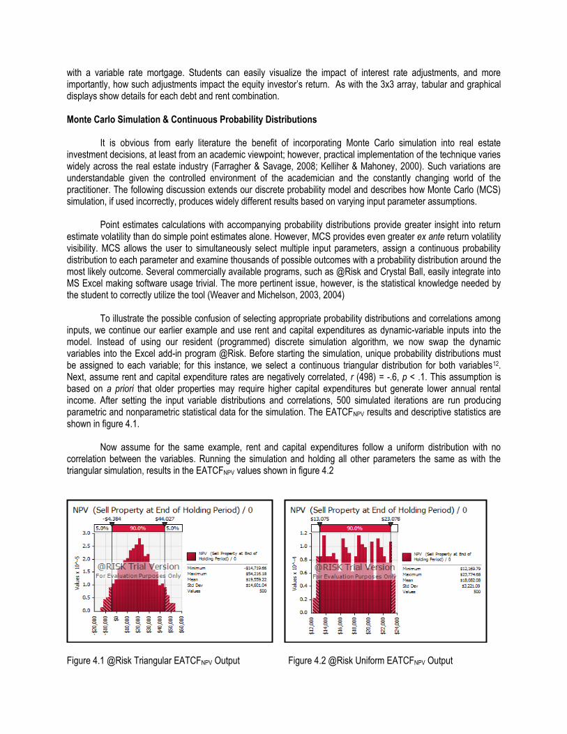
It is obvious from early literature the benefit of incorporating Monte Carlo simulation into real estate investment decisions, at least from an academic viewpoint; however, practical implementation of the technique varies widely across the real estate industry (Farragher & Savage, 2008; Kelliher & Mahoney, 2000). Such variations are understandable given the controlled environment of the academician and the constantly changing world of the practitioner. The following discussion extends our discrete probability model and describes how Monte Carlo (MCS) simulation, if used incorrectly, produces widely different results based on varying input parameter assumptions. Point estimates calculations with accompanying probability distributions provide greater insight into return estimate volatility than do simple point estimates alone. However, MCS provides even greater ex ante return volatility visibility. MCS allows the user to simultaneously select multiple input parameters, assign a continuous probability distribution to each parameter and examine thousands of possible outcomes with a probability distribution around the most likely outcome. Several commercially available programs, such as @Risk and Crystal Ball, easily integrate into MS Excel making software usage trivial. The more pertinent issue, however, is the statistical knowledge needed by the student to correctly utilize the tool (Weaver and Michelson, 2003, 2004) To illustrate the possible confusion of selecting appropriate probability distributions and correlations among inputs, we continue our earlier example and use rent and capital expenditures as dynamic-variable inputs into the model. Instead of using our resident (programmed) discrete simulation algorithm, we now swap the dynamic variables into the Excel add-in program @Risk. Before starting the simulation, unique probability distributions must be assigned to each variable; for this instance, we select a continuous triangular distribution for both variables12. Next, assume rent and capital expenditure rates are negatively correlated, r (498) = -.6, p < .1. This assumption is based on a priori that older properties may require higher capital expenditures but generate lower annual rental income. After setting the input variable distributions and correlations, 500 simulated iterations are run producing parametric and nonparametric statistical data for the simulation. The EATCFNPV results and descriptive statistics are shown in figure 4.1. Now assume for the same example, rent and capital expenditures follow a uniform distribution with no correlation between the variables. Running the simulation and holding all other parameters the same as with the triangular simulation, results in the EATCFNPV values shown in figure 4.2

Figure 4.1 @Risk Triangular EATCFNPV Output Figure 4.2 @Risk Uniform EATCFNPV Output

Results from the two simulations reveal very different outcomes. The standard deviation for EATCFNPV using

a triangular set of distributions resulted in a dispersion of $14, 501, while the standard deviation for the uniform distributions with non-correlated dynamic variables resulted in a dispersion of $3, 221. Also, the simulation using triangular distributions showed that 5% of the time, EATCFNPV was below -$4, 384, while the uniform distribution had a minimum EATCFNPV of $12,169. Clearly, this simple analogy highlights the importance of properly selecting input parameter distributions, their interdependencies and correlations. It also appears to validate the concerns highlighted from the review of literature regarding the same problem. Selecting the wrong modeling inputs provides no more accuracy than a naïve model based on subjective rationale, yet renders the illusion of possibly being more accurate.

Conclusions

The simulation model described in this paper enables students to assess real estate investment return outcomes using several approaches, including individual pro forma based point estimates and simulated point estimates with accompanying probabilistic ranges. By utilizing a student-friendly Excel based architecture, users can easily transition from point estimate calculations to more difficult concepts such as the probabilistic outcomes. Limiting the number of possible simulation variables to seven minimizes model complexity and allows users to focus uniquely on a manageable set of real estate related variables. As students become comfortable with simple discrete probabilistic simulation analysis, more advanced parameterized Monte Carlo simulation analysis can be introduced. Prerequisites for using the model include a basic foundation in real estate finance, such as those found in many undergraduate or graduate real estate investment courses.

Existing literature reveals that professionals seldom use more than simple scenario “what-if” analysis when making real estate investment decisions (Farragher & Savage, 2008). The literature also reveals that many real estate investors are unfamiliar with more advanced techniques such as Monte Carlo simulation (Foster & Lee, 2009). Combine these issues with the fact that real estate markets are highly segmented requiring considerable data extraction costs, and it is easy to understand why more advanced risk analysis has been sparingly used by professionals. Fortunately, companies such as CoStar®, LoopNet®, CoreLogic® and REIS now provide centralized data repositories covering numerous real estate market and submarket locations. Such access mitigates many of the cost concerns. These companies are also leveraging the emergence of cloud repositories and cheap end-user devices to make data access even cheaper. Indeed, the technological limitations confronted by Pyhrr (1973) during his initial research into DSS support for real estate investment volatility now seem trivial.

The model presented in this paper fits nicely between simple static pro forma statement analysis and more advanced Monte Carlo simulation. It is envisioned that such a program will help stimulate a more deliberate discussion and understanding of real estate return volatility within the classroom, thus serving as platform that encourages the adoption of more advanced risk analytics in the real estate profession. More importantly, the model is absolutely free from the instructor’s website: http://home.barton.edu/odrive/rlee/realestate_modeling. Future extensions include additional functionally to assist students in bridging the gap between simple simulated “what-if” analysis and Monte Carlo simulation. For more information, or to obtain a copy, please feel free to contact the author at rlee@barton.edu.

References

Amidu, A. R. (2011). Research in valuation decision making processes: educational insights and perspectives. Journal of Real Estate Practice and Education, 14(1), 19-34.

Brueggeman, W.B. & Fisher, J.D. (2011) Real Estate Finance and Investments, New York, NY: McGraw-Hill

Irwin.

Cox, C.J., Ingersoll, J.E. & Ross, S.A. (1985). A theory of the term structure of interest rates, Econometrica, 53(2), 385-407.

Geltner, D., Miller, N.G., Clayton, J., Eichholtz, P. (2007). Commercial Real Estate Analysis & Investments

(2ndEd.). Cengage Learning, Ohio. Graaskamp, J. A. (1969). A Practical computer service for income approach. Appraisal Journal 37, 50-57. Kelliher, C.F. & Mahoney, L.S. (2000). Using Monte Carlo simulation to improve long-term investment decisions.

The Appraisal Journal, 68 (1), 44-56. Farragher, E. and Savage, A. (2008). An investigation of real estate investment decision making Processes. Journal

of Real Estate Practice and Education, 11(1), 29-40. Farragher, E. & R. Kleiman. (1996). A Re-examination of real estate investment decision making practices. Journal

of Real Estate Portfolio Management, 2(1), 31-9.

Foster, J.J. & Lee, B.D. (2009) Sophisticated sensitivity: Can developers guess smarter? (Master’s thesis). Retrieved from MIT University, MIT Libraries Web site: http://dspace.mit.edu/handle/1721.1/54853

Greer, G. E., Kolbe, P. T. (2003). Investment Analysis for Real Estate Decisions (5th Ed.). Chicago, IL: Dearborn Financial Publishing.

Hoesli, M., Jani, E. & Bender, A. (2006). Monte Carlo simulations for real estate valuation. Journal of Property

Investment and Finance, 24(2), 102-22. Li, H.L. (2000). Simple computer applications improve the versatility of discounted cash flow analysis. The

Appraisal Journal, 68 (1), 86-92.

Ling, D. C. & Archer, W. R. (2010). Real Estate Principles: A Value Approach (3rd Ed.). New York, NY: McGraw-Hill Irwin.

Meredith, Shafer & Turbin (2002). Quantitative Business Modeling, Ohio: South-Western College Publishing. Myers, S. (1974). Interactions in corporate financing and investment decisions – Implications for capital budgeting.

Journal of Finance, 29(1), 1-25. Pyhrr, S.A. (1973). A computer simulation model to measure risk in real estate investment. Journal of the American

Real Estate and Urban Economics Association, 1(1), 48-78.

Wofford, L.E. (1978). A simulation approach to the appraisal of income producing real estate. Journal of the American Real Estate and Urban Economics Association, 6(4), 370-394.

Slade, Barrett, A. (2006). Property risk assessment: a simulation approach. The Appraisal Journal, 74 (4). Weaver, W. and Michelson, S. (2003). A practical tool to assist in analyzing risk associated with income

capitalization approach valuation or investment analysis. The Appraisal Journal, 71(4), 335-344.

Weaver, W. and Michelson, S. A (2004). A pedagogical tool to assist in teaching real estate investment risk analysis. Journal of Real Estate Practice and Education, 7(1), 45-52.

Appendices Appendix A: Commercial Real Estate Valuation Software Vendors

Software Vendor Web Address

Argus Valuation DCF http://www.argussoftware.com/en/products/ARGUSDCF/default.aspx

planEASe http://www.planease.com/

Narrative Appraisal System http://www.narrative1.com/

Yardi PropertyVMF http://www.yardi.com/product/YardiPropertyVMF.aspx

Real Data http://www.realdata.com/p/reia/reiafamily.shtml

REIWISE http://www.reiwise.com/

Investment Analyst http://www.realestatevaluationsoftware.dcfsoftware.com/

Cash Flow Analyzer Pro http://www.rentalsoftware.com/

Marshall & Swift http://www.marshallswift.com/c-1-residential-products.aspx

(Property Replacement Cost Estimates)

Advantage Software LCC http://www.invest-2win.com/

CREmodel http://www.cremodel.com/?gclid=CInQvLLmjaUCFRBL2godhGLcPA

REALBENCH http://www.realbench.net/

Appendix B: Model Input Parameters and Dynamic Variables

Inputs Variables and Parameters (User Defined)

Input Derivation

Gross Rent (GR) The initial going-in rent for the property

Property Price (P) Price paid for the property

Vacancy Rate (VR) The annual percentage vacancy rate for the property

Building Appraised Property Tax Value

Taxing municipally appraised tax value for the property structure

Land Appraised Value Taxing municipally appraised value of land

Property Tax Rate Tax rate per $100 assessed on the property

Rental Growth (Decline) Rate The implied or assumed ex-ante growth rate of rental income

Property Growth (Decline) Rate The implied or assumed ex-ante property appreciation rate (or decrease)

Years Depreciation Number of years the property is depreciated on a straight-line basis

Going-in yearly Insurance Premium The annual property insurance premium(s) on the property

Yearly Insurance Premium Rate increase (decline)

Annual increase or decrease in insurance premiums

Annual Debt Service (DS) Annual debt service = M =12 x (P [ rd (1 + rd)n ] / [ (1 + rd)n - 1]), where P = principle amount, rd is the per-period interest rate and n is the number of periods

Going in Loan-to-Value Ratio (LTV) The user specified ratio of debt to value

Rate of Debt (rd) The user specified cost of debt

Capital Expenditure Rate per year The user specified annual rate of capital expenditures as a percentage of property value

Long Term Capital Gains Tax Rate Investor’s unique long term capital gains tax rate as specified by IRS guidelines

Short Term Capital Gains Tax Rate Investor’s unique short term capital gains tax rate as specified by IRS guidelines

Ordinary Income Tax Rate Investor’s ordinary income tax rate as specified by IRS guidelines

Reinvestment Rate (MIRR) Modified internal rate of return

Risk free of 10-Year T-bonds rf = risk free rate on equivalent holding period Treasury Securities

Equity risk Premium rp = equity risk premium above the investor’s risk free rate (rf)

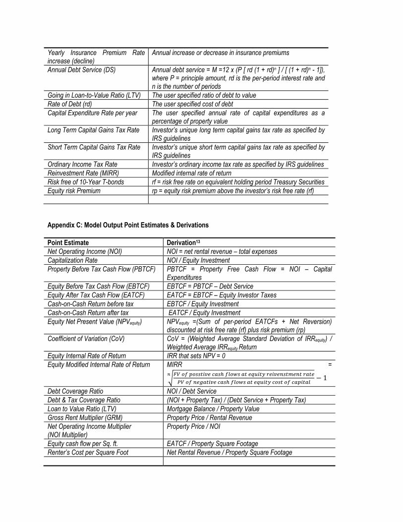
Appendix C: Model Output Point Estimates & Derivations

Point Estimate Derivation13

Net Operating Income (NOI) NOI = net rental revenue – total expenses

Capitalization Rate NOI / Equity Investment

Property Before Tax Cash Flow (PBTCF) PBTCF = Property Free Cash Flow = NOI – Capital Expenditures

Equity Before Tax Cash Flow (EBTCF) EBTCF = PBTCF – Debt Service

Equity After Tax Cash Flow (EATCF) EATCF = EBTCF – Equity Investor Taxes

Cash-on-Cash Return before tax EBTCF / Equity Investment

Cash-on-Cash Return after tax EATCF / Equity Investment

Equity Net Present Value (NPVequity) NPVequity =(Sum of per-period EATCFs + Net Reversion) discounted at risk free rate (rf) plus risk premium (rp)

Coefficient of Variation (CoV) CoV = (Weighted Average Standard Deviation of IRRequity) / Weighted Average IRRequity Return

Equity Internal Rate of Return IRR that sets NPV = 0

Equity Modified Internal Rate of Return MIRR =

√

Debt Coverage Ratio NOI / Debt Service

Debt & Tax Coverage Ratio (NOI + Property Tax) / (Debt Service + Property Tax)

Loan to Value Ratio (LTV) Mortgage Balance / Property Value

Gross Rent Multiplier (GRM) Property Price / Rental Revenue

Net Operating Income Multiplier (NOI Multiplier)

Property Price / NOI

Equity cash flow per Sq. ft. EATCF / Property Square Footage

Renter’s Cost per Square Foot Net Rental Revenue / Property Square Footage

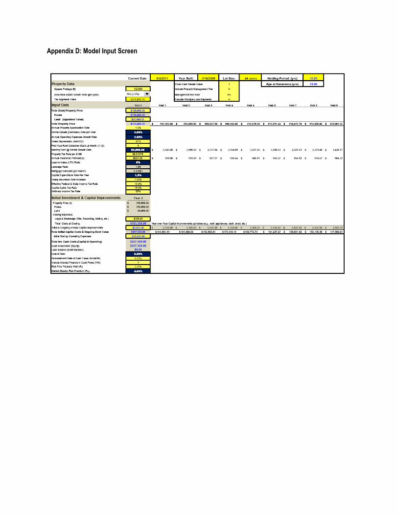
Appendix D: Model Input Screen

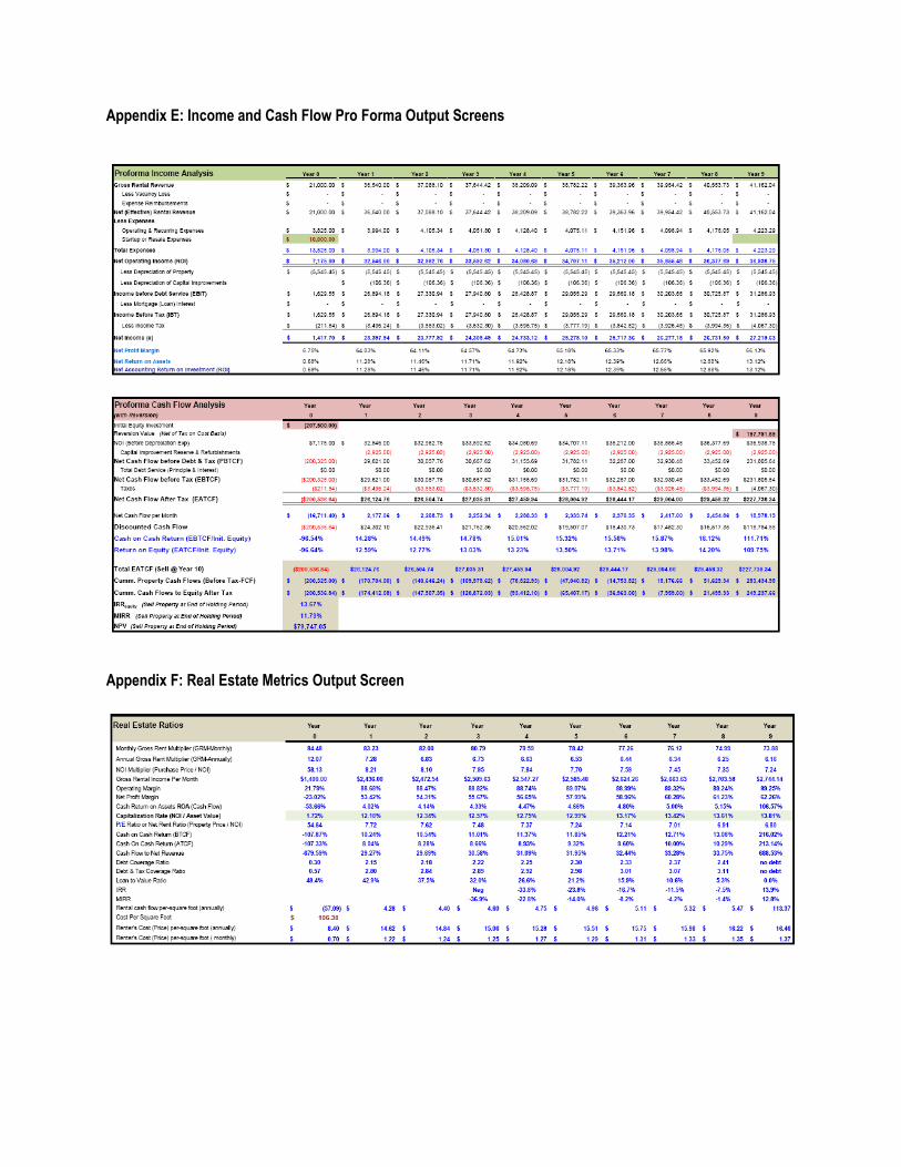
Appendix E: Income and Cash Flow Pro Forma Output Screens

Appendix F: Real Estate Metrics Output Screen

Appendix G: Mortgage Output Screen

Appendix H: Annual Recurring Expenses Screen

Appendix I: ROE and IRR Simulation and Output Results

Simulate ROE & IRR

Appendix J: Reversion Output Screen & Graphics

Endnotes

1 Direct capitalization uses only a single year’s net income, or the average of several years, and a market defined

capitalization rate.

2 In retrospect, this is the primary reason they chose to simplify the discussion to only year-end cash flow and a

single reversion values. The authors avoid the discussion of risks associated with multiple input parameters and the

difficult realization of validating the data’s integrity.

3 The authors use Paris France real estate indexes for pricing datasets.

4 Many of these software applications run on top of Excel and have Excel or Visual Basic code base.

5 As we will discuss later, and as noted in the literature review, Monte Carlo simulation requires considerable

understanding of inter-variable relationships and correlations between the modeling inputs.

6 Since the model is based on Excel, other metrics can be easily added by the instructor or user.

7 Appendices B and C provide a list of all financial real estate metrics used in the model.

8 Excel for calculating the mortgage constant: PMT(rate,nper,pv,fv,type) where pv=-1, fv=0.

9 For the sake of simplicity and brevity, only the primary model equations are shown and discussed. Details for each

intermediate parameter or variable (input and output) can be found in Appendix C.

10 See Appendix B for the debt service equation.

11 The coefficient of variation is defined as the ratio of standard deviation over the expected mean return.

12 Triangular distributions use a minimal, most likely and maximum probability distribution, similar to a worse case,

most likely case best case “what-if” scenario. Thus many analysts may find such distributions a good starting

point for assigning probability inputs.

13 All metrics are on an annualized basis.