Abstract—Aim of this research is to study periodic modeling

of 15 days cumulative rainfall time series. The study was

undertaken using 25 years (1977–2001) data of Purajaya

region. The series of the daily rainfall data assumed was trend

free. The periodic component of 15 days cumulative rainfall

time series could be represented by using 253 harmonic

expressions. The stochastic component of the 15 days

cumulative rainfall was using the 3rd

order autoregressive

model. Validation of generated 15 days cumulative rainfall

series was done by comparing between the generated with the

measured rainfall series. The correlation coefficient between

the generated or synthetic rainfall series with the measured

rainfall series with the number of the data N is equal to 512

days for 25 years was found to be 0.99996. Therefore,

developed model could be used for future prediction of 15

days cumulative rainfall time series.

Index Terms - 15 days cumulative rainfall, fast Fourier transform,

autoregressive model, least squares method.

I. INTRODUCTION

To design water consuming of irrigation, detailed

information about the rainfall with respect to time is required.

To provide long sequence record of rainfall data was very

difficult, so sometime to extend the rainfall record, generating

the synthetic rainfall record is necessary. Various methods

have been used by Engineers and scientists to provide this

information. Most the existing methods are either

deterministic or probabilistic in nature [3] and [2]. While the

former methods do not consider the random effects of various

input parameter, the later method employ the concept of

probability to the extent that the time based characteristics of

rainfalls are ignored. With the ever increasing demand for

accuracy of analyzing rainfall data, these methods are no

longer sufficient.

The rainfalls are periodic and stochastic in nature, because

they are affected by climatological parameter, i. e., periodic

and stochastic climate variations are transferred to become

periodic and stochastic components of rainfalls. Hence the

Ir. Ahmad Zakaria, Ph.D., is working as senior lecturer at Department

of Civil Engineering, Faculty of Engineering, Lampung University, Indonesia.

He area of interest is in the field of physical and numerical modeling of wave

propagation and signal processing. He is the corresponding author.

(Phone:+62-07217502636; Fax: +603-86567123; email: ahmadzakaria

@unila.ac.id).

rainfalls should be computed considering both the periodic

and the stochastic parts of the process. Considering all other

factors known or assumed that the rainfall is a function of the

stochastic variation of the climate. Hence periodic and

stochastic analysis of rainfall time series will provide a

mathematical model that will account for the periodic and

stochastic parts and will also reflect the variation of rainfalls.

During the past years, some researches that study the

periodic and stochastic modeling have been published by [4]

[5] [7] [8] [9] [10].

Aim of this research is to generate the sequences of 15 days

cumulative rainfall time series for Purajaya station using fast

Fourier transform and least squares methods. The model can

be used to provide synthetic and reasonably rainfall data for

planning the irrigation or water resource projects in the future.

II. MATERIALS AND METHODS

2.1. Study Area

The study area comes under the humid region of the sub-

district of West Lampung, Profince of Lampung, Indonesia.

2.2. Collection of Rainfall Data

Daily rainfall data of Purajaya region was collected from

Indonesian Meteorological, Climatological and Geophysical

Agency, Profince of Lampung. Rainfall data for a period of 25

years (1977-2001) was used in the study.

The mathematical procedure adopted for formulation of a

predictive model has been discussed as follows: The principal

aim of the analysis was to obtain a reasonable model for

estimating the generation process and its parameters by

decomposing the original data series into its various

components.

Generally a time series can be decomposed into a

deterministic component, which could be formulated in

manner that allowed exact prediction of its value, and a

stochastic component, which is always present in the data and

can not strictly be acounted for as it is made by random

effects. The time series X(t) was represented by a

decomposition model of the additive type [5][7][8], as folows,

( ) ( ) ( ) ( )tS+tP +tT=tX (1)

A study modeling of 15 days cumulative rainfall

at Purajaya Region, Bandar Lampung, Indonesia

Ahmad Zakaria*

INTERNATIONAL JOURNAL OF GEOLOGY Issue 4, Volume 5, 2011

101

Where, T (t) is the component of trend, t = 1, 2, 3... N. P (t)

is the periodic components, and S (t) is the stochastic

components.

In this research, the rainfall data is assumed to have no trend.

So this equation can be presented as follows,

( ) ( ) ( )t S+tPtX ≈ (2)

(2) is an equation to obtain the representative periodic and

stochastic models of 15 days cumulative rainfall series.

2.3. Spectral Method

Spectral method is one of the transformation method

which generally used in applications. it can be presented as

Fourier transform [6][8][9][10] as follows,

( ) ( )∑−

−2/

2/

...2.

.2

N=n

N=n

m

nmM

iπ

etPπ

∆t=fP (3)

Where P (t) is a 15 days cumulative rainfall data series

in time domain and P (fm) is a 15 days cumulative rainfall data

series in frequency domain. The t is a series of time that

present a length of the rainfall data to N, The fm is a series of

frequencies.

Based on the rainfall frequencies resulted using Equation

(3), amplitudes as functions of the rainfall frequencies can be

generated. The maximum amplitudes can be obtained from the

amplitudes as significant amplitudes. The rainfall frequencies

of significant amplitudes used to simulated synthetic rainfalls

are assumed as significant rainfall frequencies. The significant

rainfall frequencies resulted in this study is used to calculate

the angular frequencies (ωr) and obtain the periodic

components of Equation (4) or (5).

2.4. Periodic Components

The periodic component P(t) concerns an oscillating

movement which is repetitive over a fixed interval of time

(Kottegoda 1980). The existence of P(t) was identified by the

fourier transformation method. The oscillating shape verifies

the presence of P(t) with the seasonal period P, at the

multiples of which peak of estimation can be made by a

Fourier Analysis. The frequencies of the spectral method

clearly showed the presence of the periodic variations

indicating its detection. The periodic component P(t) was

expressed in Fourier series [4] as follows,

( ) t)(ωB+t)(ωA+ S=tP r

kr=

r=

rr

kr=

r=

ro . cos.sinˆ

11

∑∑

(4)

Equation (4) could be arranged to be Equation as follows,

( ) t)(ωB+t)(ωA=tP r

k=r

=r

rr

+k=r

=r

r .cos.sinˆ

1

1

1

∑∑

(5)

Where ( )tP is the periodic component, (t)P̂ is the

periodic component of the model, So = Ak + 1 is the mean of the

rainfall time series rω is the angular frequency. Ar and Br are

the coefficients of Fourier components.

2.5. Stochastic Components

The stochastic component was constituted by various

random effects, which could not be estimated exactly. A

stochastic model in the form of autoregressive model was used

for the presentation in the time series. This model was applied

to the S (t) which was treated as a random variable.

Mathematically, an autoregressive model of order p can be

written as:

( ) ( )∑ −p

=k

k ktSb+ε=tS1

. (6)

Equation (6) may be arranged as,

( ) ( ) ( ) ( )ptSb++tSb+tSb+ε=tS p −−− ....2.1. 21 (7)

Where, br is the parameter of the autoregressive model. ε is

the constant of random numbers. r = 1, 2, 3, 4,..., p is the order

of stochastic components. To get the parameter of the

autoregressive model and the constant of random number, least

squares method can be applied.

2.6. Least Squares Method

2.6.1. Analysis of periodic components

In curve fitting, as an approximate solution of periodic

components P (t), to determine Function ( )tP ˆ of Equation

(4) and (5), a procedure widely used is least squares method.

From Equation (5) we can calculate sum of squares [4] as

follows,

Sum of squares = J = ( ) ( ){ }∑ −m=t

=t

tPtP1

2ˆ

(8)

Where J is depends on Ar Br, and ωr. A necessary condition for

J be minimum is as follows,

INTERNATIONAL JOURNAL OF GEOLOGY Issue 4, Volume 5, 2011

102

0=B

J=

A

J

rr ∂∂

∂∂

with r = 1,2,3,4,5,...,k (9)

Using the least squares method, we can find equations as

follow,

a. mean of series,

S

o=A

k+1 (10)

b. amplitudes of significant harmonics,

2

rrr B+A=C 2 (11)

c. phases of significant harmonics,

r

rr

A

B=φ arctan (12)

Mean of 15 days cumulative rainfalls, amplitudes, and phases

of significant harmonics can be substituted into an equation as

follow,

( )∑ −k=r

=r

rrro φtωCosC+S=tP1

..)(ˆ (13)

Equation (13) is harmonic model of the 15 days cumulative

rainfall where can be found based on the 15 days cumulative

rainfall data series of Purajaya.

2.6.2. Analysis of stochastic components

Based on the results of the simulations obtained from

periodic rainfall models, stochastic components S (t) can be

generated. The stochastic component is the difference between

rainfall data series with calculated rainfall series obtained from

periodic model. Stochastic series as a residual rainfall series,

which can be presented as follows,

( ) ( ) ( )tP -tXtS ≈ (14)

(14) can be solved by using the same way with the way that

used to get periodic rainfall series components. Following (8)

and (9), stochastic models (7) can be arranged to be as follows,

Sum squares of error = J = ( ) ( ){ }∑ −m=t

=t

tStS1

2ˆ

(15)

Where J is sum square of error. It depends on the ℇ and br

values, where the coefficients can only be minimum value if it

satisfies the equation as follows,

0=b

J=

ε

J

r∂∂

∂∂

with r = 1, 2, 3, 4, 5, ..., p (16)

In the next, by using (16) stochastic parameters ε and br of the

residual rainfall data can be calculated.

III. RESULTS AND DISCUSSION

For testing the statistical characteristics of daily rainfall series,

25 years data (1977-2001) of daily rainfall from station

Purajaya was taken. The statistical characteristic of the annual

mean and maximum rainfall of daily rainfall series were

estimated. Figure 1 shows the daily rainfall time series.

Figure 1. Daily rainfall time series for 25 years from Purnajaya station.

From Figure 1 is presented mean annual daily rainfall

values vary from 2 mm in the year of 1986 to 12.5 mm in the

year of 1977. Maximum annual daily rainfall values vary from

35 mm in the year of 1986 to 152.9 mm in the year of 1992.

For annual cumulative daily rainfall indicate minimum value

of 552.5 mm in the year of 1989 and maximum value of

4308.9 mm in the year of 1996 with mean annual cumulative

daily rainfall value of 2553.5 mm. Based on daily rainfall time

series, a series of 15 days cumulative rainfall was generated as

presented in Figure 2,

INTERNATIONAL JOURNAL OF GEOLOGY Issue 4, Volume 5, 2011

103

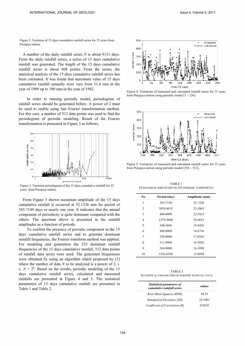
Figure 2. Variation of 15 days cumulative rainfall series for 25 years from

Purajaya station.

A number of the daily rainfall series N is about 9131 days.

From the daily rainfall series, a series of 15 days cumulative

rainfall was generated. The length of the 15 days cumulative

rainfall series is about 608 points. From the series, the

statistical analysis of the 15 days cumulative rainfall series has

been estimated. It was found that maximum value of 15 days

cumulative rainfall annually were vary from 31.4 mm in the

year of 1989 up to 390 mm in the year of 1982.

In order to running periodic model, periodogram of

rainfall series should be generated before. A power of 2 must

be used to enable using fast Fourier transformation method.

For this case, a number of 512 data points was used to find the

periodogram of periodic modeling. Result of the Fourier

transformation is presented in Figure 3 as follows,

Figure 3. Variation periodogram of the 15 days cumulative rainfall for 25

years from Purajaya station.

From Figure 3 shown maximum amplitude of the 15 days

cumulative rainfall is occurred at 52.1326 mm for period of

365.7149 days or nearly one year. It indicates that the annual

component of periodicity is quite dominant compared with the

others. The spectrum above is presented in the rainfall

amplitudes as a function of periods.

To confirm the presence of periodic component in the 15

days cumulative rainfall series and to generate dominant

rainfall frequencies, the Fourier transform method was applied.

For modeling and generation the 253 dominant rainfall

frequencies of the 15 days cumulative rainfall, 512 data points

of rainfall data series were used. The generated frequencies

were obtained by using an algorithm which proposed by [1]

where the number of data N to be analyzed is a power of 2, i.

e. N = 2k. Based on the results, periodic modeling of the 15

days cumulative rainfall series, calculated and measured

rainfalls are presented in Figure 4 and 5. The statistical

parameters of 15 days cumulative rainfall are presented in

Table 1 and Table 2.

Figure 4. Variations of measured and calculated rainfall series for 25 years

from Purajaya station using periodic model (1 ~ 256).

Figure 5. Variations of measured and calculated rainfall series for 25 years

from Purajaya station using periodic model (256 ~ 512).

TABLE 1

10 MAXIMUM AMPLITUDES OF 253 PERIODIC COMPONENTS

No Period (day) Amplitude (mm)

1 365.7149 52.1326

2 3839.8635 23.5065

3 480.0000 22.5415

4 1279.9848 20.4015

5 548.5686 19.4426

6 960.0000 18.6756

7 320.0000 17.0262

8 511.9988 16.5882

9 384.0000 16.1898

10 1536.0109 15.8058

TABLE 2

STATISTICAL PARAMETERS OF PERIODIC RAINFALL DATA

Statistical parameters of

cumulative rainfall series values

Root Mean Squares (RMS) 30.53

Standard of Deviation (SD) 18.3401

Coefficient of Correlation (R) 0.9239

INTERNATIONAL JOURNAL OF GEOLOGY Issue 4, Volume 5, 2011

104

Coefficient of Variance 0.6006

Coefficient of Skewness (Cs) 0.2887

Coefficient of Curtosis (Cc) 2.0702

Based on the results of periodic modeling, the residual of

cumulative rainfall was generated by using Equation (14) is

presented in Figure 6 and Figure 7.

Figure 6. Residual variation of measured and calculated 15 days cumulative

rainfall for Purajaya station (1 ~ 256).

Figure 7. Residual variation of measured and calculated 15 days cumulative

rainfall for Purajaya station (256 ~ 512).

TABLE 3

AUTOREGRESSIVE PARAMETERS FOR 3TH ORDER ACCURACIES

autoregressive

parameters value

ε 0

b1 0.9562

b2 0.9955

b3 −0.9550

Autoregressive parameters presented in Table 3 results the

best fit for the stochastic model of the residual rainfall. Based

on the results, comparison between measured and calculated

residual 15 days cumulative rainfall are presented in Figure 8

and Figure 9. These results show that the calculated results

have good agreement with measured results.

Figure 8. Variations of measured and calculated residual 15 days

cumulative rainfall for Purajaya station (1 ~ 256).

Figure 9. Variations of measured and calculated residual 15 days cumulative

rainfall for Purajaya station (256 ~ 512).

A comparison between the measured 15 days cumulative

rainfall and the calculated 15 days cumulative rainfall of the

periodic and stochastic modeling as shown in Figure 10 and

Figure 11 indicate that, the calculated 15 days cumulative

rainfall of the periodic and stochastic models gives highly

accurate results.

INTERNATIONAL JOURNAL OF GEOLOGY Issue 4, Volume 5, 2011

105

Figure 10. Variations of measured and calculated 15 days cumulative rainfall

series for Purajaya station using periodic and stochastic model (0 ~ 256).

Figure 11. Variations of measured and calculated 15 days cumulative

rainfall series for Purajaya station using periodic and stochastic model (256

~ 512).

For modeling of the periodic rainfall provides the

correlation coefficient R is 0.9239. For modeling of the

stochastic rainfall is using 3rd

orders autoregressive model

gives the correlation coefficient R is 0.9997. For modeling of

stochastic and periodic 15 days cumulative rainfall giving the

correlation coefficient between the data and the model

increases to be 0.99996. The coefficient correlation R is

almost close to 1. This shows that the model of periodic and

stochastic 15 days cumulative rainfall is almost close to the

pattern of rainfall 15 days cumulative rainfall data. It indicates

that the periodic and stochastic models can give more accurate

and significant result.

Variation of the correlation coefficient of the stochastic

model R(S), the correlation coefficient of the periodic and

stochastic model R(P+S) and the error of the 15 days

cumulative rainfall versus the orders of the autoregressive

model can be seen in the Fig. 12.

Figure 12. Variations of error, correlation coefficients of stochastic (S),

periodic and stochastic (P+S) models for different stochastic orders.

Based on, the results presented in Fig. 12 shows that using

the 3rd

order autoregressive model can give better accuracy

results than the 2nd

order autoregressive model. For the

accuracy of the 4th order up to the accuracy of the 10

th order

did not provide more significant results, if it is compared with

the accuracy of the 3rd

order autoregressive model. So in this

research, the stochastic component is modeled using the 3rd

order autoregressive model. The correlation coefficient R and

the error (%) for modeling of the synthetic periodic rainfall

give the correlation coefficient is equal to 0.9239 and the error

is equal to 28%. For modeling the periodic and stochastic

rainfalls provides the correlation coefficient is equal to

0.99996 and the error is equal to 0.79 %.

The 15 days cumulative rainfall modeling in this research

can be compared to the synthetic rainfall modeling such as

have been done by [5] and [7], where in the modeling they

only use a few periodic and stochastic parameters. To model

the synthetic rainfall, in his work, [5] using up to six harmonic

components and with stochastic components using 3rd

order

autoregressive model. For [7], in the research, they use only

three harmonic components with stochastic component for 1st

order autoregressive model. In this research, more complex

solution is conducted than previous researches. Even though

by using 253 periodic components, the harmonic modeling of

15 days cumulative rainfall in this research is done easily.

Because, by applying the fast Fourier transforms (FFT), the

dominant rainfall frequencies of the 15 days cumulative

rainfall can be generated quickly.

Behavior of the stochastic 15 days cumulative rainfall can

be seen such as presented in Fig. 8 and Fig. 9. The stochastic

components series is the difference between the 15 days

cumulative rainfall data with the periodic model series. From

the figures they present that the stochastic component

fluctuates in value from - 68.6 mm up to 68.6 mm. The

correlation coefficient of stochastic models with the accuracy

of the 3rd

order is equal to 0.9997, while the 1st order

autoregressive model of the stochastic model is equal to

0.9838. The result is better when compared with the results

presented by [7] which uses stochastic model for the accuracy

INTERNATIONAL JOURNAL OF GEOLOGY Issue 4, Volume 5, 2011

106

of the 1st order and give the coefficient correlation for

stochastic model of 0.9001.

By using the 253 periodic components and 3rd

order

autoregressive model yield the simulation model of 15 days

cumulative rainfall accurately, with a correlation coefficient is

equal to 0.99996. The correlation coefficient presented in Fig.

12 is proof that periodic and stochastic models (P + S) of 15

days cumulative rainfall has a very good correlation and

accurate results when compared with only using periodic

model (P) that generates correlation coefficient of 0.9239. This

result also looks much better when compared to the research

done by [7], where the model only using the 3 periodic

components with the 1st order accuracy of stochastic

component with the correlation coefficient is 0.9961.

The results also better even though compared with the

research for the daily rainfall series of 25 years rainfall data

which have been done by [9], where by using the 253

harmonic components, average of the correlation coefficient of

periodic model is about 0.9576. In [10] by using the 253

harmonic components and the 2nd

order autoregressive model,

average of the correlation coefficient of stochastic model is

about 0.9989 and for the correlation coefficient of periodic

and stochastic models is about 0.99993.

IV. CONCLUSION

The spectrum of the 15 days cumulative rainfall time series

generated by using the FFT method is used to simulate the

synthetic 15 days cumulative rainfall. By using the least

squares method, the 15 days cumulative rainfall time series can

be produced synthetic rainfall quickly. By using 253 periodic

components and 3rd

order stochastic components, the 15 days

cumulative rainfall model from Purajaya station can be

produced accurately with the correlation coefficient of

0.99996.

ACKNOWLEDGMENT

This paper is part of the research work carried out under the

project funded by the DIPA Unila, Lampung University,

Indonesia.

REFERENCES

[1] Cooley, James W. Tukey, John W. (1965). An Algorithm for the

machine calculation of Complex Fourier Series. Mathematics of

Computation, 199-215.

[2] Yevjevich, V. (1972). Structural analysis of hydrologic time series,

Colorado State University, Fort Collins.

[3] Kottegoda, N. T. (1980). Stochastic Water Resources Technology.

London: The Macmillan Press Ltd.

[4] Zakaria, A. (1998). Preliminary study of tidal prediction using Least

Squares Method. Thesis (Master). Bandung Institute of Technology,

Bandung, Indonesia.

[5] Rizalihadi, M. (2002). The generation of synthetic sequences of monthly

rainfall using autoregressive model. Jurnal Teknik Sipil Universitas

Syah Kuala, 1(2), 64-68.

[6] A. Zakaria, A. (2003). Numerical modelling of wave propagation using

higher order finite-difference formulas, Thesis (Ph.D.), Curtin

University of Technology, Perth, W.A., Australia.

[7] Bhakar, S. R., Singh, Raj Vir, Chhajed, Neeraj, and Bansal, Anil

Kumar. (2006). Stochstic modeling of monthly rainfall at kota region.

ARPN Journal of Engineering and Applied Sciences, 1(3), 36-44.

[8] Zakaria, A. (2008). The generation of synthetic sequences of monthly

cumulative rainfall using FFT and least squares method. Prosiding

Seminar Hasil Penelitian & Pengabdian kepada Masyarakat,

Universitas Lampung, 1, 1-15.

[9] Zakaria, A. (2010). A study periodic modeling of daily rainfall at

Purajaya region. Seminar Nasional Sain & Teknologi III, 18-19 October

2010, Lampung University, 3, 1-15.

[10] Zakaria, A. (2010). Studi pemodelan stokastik curah hujan harian dari

data curah hujan stasiun Purajaya. Seminar Nasional Sain Mipa dan

Aplikasinya, 8-9 December 2010, Lampung University, 2, 145-155.

INTERNATIONAL JOURNAL OF GEOLOGY Issue 4, Volume 5, 2011

107