Embed Size (px)
Citation preview
A Study of Closing Costs for FHA Mortgages
U.S. Department of Housing and Urban Development
Office of Policy Development and Research
A Study of Closing Costs for FHA Mortgages
Prepared for:U.S. Department of Housing and Urban DevelopmentOffice of Policy Development and Research
Prepared by:Susan E. Woodward, Ph.D.for the Urban InstituteWashington, DC
May 2008
ACKNOWLEDGMENTS
The contents of this report are the view of the contractor, myself, Susan E. Woodward, and do not necessarily reflect the views or policies of the U.S. Department of Housing and Urban Development, the U. S. government, the Urban Institute, its trustees or its funders. I am especially grateful to Bill Reid, who collaborated at every step of the study, and to Harold Bunce, Bill Reeder, and Kurt Usowski and their colleagues in the Office of Policy Development and Research at HUD for their assistance and their patience regarding requests for more data and yet more data for this project, for their careful review of the data and results, and advice on FHA files. I also wish to thank especially Harold Katsura, previously of the Urban Institute, now of HUD, for his meticulous oversight of collection of data from HUD-1 settlement statements and subsequent thorough reviews of the data. In many ways, data collection was the lion’s share of the work in this effort.
Special thanks go also to Ned Gramlich, who read a draft in summer of 2007. His enthusiasm and encouragement meant a lot to all of us. And to Bob Van Order, who reviewed a draft in early 2008 and provided additional encouragement. Marge Turner, of the Urban Institute, was a welcome influence, especially in emboldening the prose in the executive summary. Thanks also to Doug Wissoker, also of the Urban Institute, for advice on and review of econometric issues, for replicating and confirming the results, and for calculating bootstrapped standard errors, to Signe-Mary McKernan for many constructive suggestions and for keeping us organized and moving forward, and to Katie Vinopal for meticulous and untiring research assistance. Very special thanks to my husband, Bob Hall, who in so many ways is also my most important colleague. He indulged me in unlimited conversation at breakfast, dinner and while hiking about the institutions, price theory, and econometrics of mortgage lending. All remaining errors are my own.
ABOUT THE AUTHOR
Dr. Woodward, an expert in financial economics, has held appointments in both academia and government. She has been on the faculties of the University of California at Los Angeles and at Santa Barbara and the University of Rochester’s Simon School. She has also served as Chief Economist of the Securities and Exchange Commission, Chief Economist of the Department of Housing and Urban Development, and Senior Staff Economist for Financial Markets and Institutions at the Council of Economic Advisers. Dr. Woodward is currently the founder and chairman of Sand Hill Econometrics, Inc. in Palo Alto, California. The Urban Institute is a nonprofit, nonpartisan policy research and educational organization that examines the social, economic, and governance problems facing the nation. The views expressed are those of the author and should not be attributed to the Urban Institute, its trustees, or its funders.
A Study of Closing Costs for FHA Mortgages
CONTENTS
EXECUTIVE SUMMARY .....................................................................................................VIII
Lenders and Mortgage Brokers............................................................................................ viii Title Services ........................................................................................................................ xii Real Estate Agent Services .................................................................................................. xiii Conclusions and Implications .............................................................................................. xiii
PART A: BACKGROUND .......................................................................................................... 1
Chapter I: Introduction................................................................................................................ 1 Motivation and Background ................................................................................................... 1 The Data.................................................................................................................................. 2 The Issues................................................................................................................................ 2 Analysis of a Mortgage Rate Sheet......................................................................................... 4 The Logic of “Points” ........................................................................................................... 10
Chapter II: Review of Previous Research................................................................................. 13 Research in Mortgage Lending Costs ................................................................................... 13 Research on Defaults, Prepayment Rates, and Discrimination............................................. 16 Findings from the Auto Loan Market ................................................................................... 18 Research Outside Lending .................................................................................................... 18 The Importance of Shopping Behavior................................................................................. 19 Fully Informed versus Partially Informed Markets .............................................................. 20
PART B: LENDER AND BROKER CHARGES .................................................................... 22
Chapter III: A Descriptive Approach to Lender/Broker Charges ............................................. 22 Loan Origination Fees........................................................................................................... 22
Chapter IV: Econometric Issues ............................................................................................... 33Constructing a Single Metric of Loan Cost .......................................................................... 33 Estimating YSPs ................................................................................................................... 34 Treatment of Subsidized Loans ............................................................................................ 36 Model for Estimating Yield-Spread Premiums..................................................................... 36 Estimating Credit Scores....................................................................................................... 37 Bootstrapped Standard Errors ............................................................................................... 37 Remaining Econometric Issues............................................................................................. 38
iii

A Study of Closing Costs for FHA Mortgages
Chapter V: Loan Origination Fees in Relation to Loan and Borrower Characteristics ............ 40 Basic Findings....................................................................................................................... 43 Credit Scores......................................................................................................................... 44 Borrower Race ...................................................................................................................... 45 Education .............................................................................................................................. 48 State Differences ................................................................................................................... 50 Brokered versus Direct Loans............................................................................................... 53 Loan Counseling ................................................................................................................... 55
Chapter VI: Sources of Complexity and Confusion: Yield-spread Premiums, Discount Points, and Seller Contributions ........................................................................................................... 57
Yield-Spread Premiums ........................................................................................................ 57Discount Points ..................................................................................................................... 60 Seller Contribution................................................................................................................ 63 Confusion Differences by Lender Type................................................................................ 65
Chapter VII: A Source of Simplicity: The “No-cost” Loans .................................................... 70 Chapter VIII: Costs of Doing Business: Defaults and Dry Holes ............................................ 74
Defaults and Delinquencies .................................................................................................. 74 Dry-Hole Costs ..................................................................................................................... 76
Chapter IX: Reflections on the Findings .................................................................................. 81
PART C: TITLE CHARGES AND REAL ESTATE TRANSACTION FEES .................... 86
Chapter X: Title Charges .......................................................................................................... 86 Controversies in Title Insurance ........................................................................................... 86 What the Data Reveal ........................................................................................................... 88 Variations among and within States ..................................................................................... 90 Relation of Title Charges with Loan and Borrower Characteristics................................... 102 Reflections on the Findings ................................................................................................ 104
Chapter XI: Real Estate Transaction Fees .............................................................................. 107
APPENDIX I: ECONOMETRIC MEASURES I-1
APPENDIX II: REFERENCES II-1
APPENDIX III: DATA III-1
iv

A Study of Closing Costs for FHA Mortgages
APPENDIX IV: REVEW OF PRIOR RESEARCH ON TITLE FEES IV-1
APPENDIX V: VARIATION IN TITLE CHARGES BY STATE V-1
v
A Study of Closing Costs for FHA Mortgages
LIST OF EXHIBITS Table 1-1 A Typical Rate Sheet 6
Figure 3-1 Coupon Rate versus YSP Divided by Loan Amount for Loans
Figure 3-2 Upfront Cash and Loan Amount for Loans with Reported YSPs
Figure 3-3 Yield-Spread Premium versus Upfront Cash for Brokered
Figure 3-4 Upfront Cash Divided by Loan Amount versus YSP Divided by
Figure 3-5 Total Charges (Upfront Cash plus YSP) versus YSP for Brokered,
Figure 3-6 Total Charges (Upfront Cash plus YSP) versus YSP, each Divided
Figure 3-7 Coupon Rates versus Upfront cash for Nonsubsidized Loans
Figure 3-9 Yield Spread Premium versus Coupon Rate Taken from Rate Sheets for Twelve National, Anonymous Wholesale Lenders for
Table 1-2 Means and Standard Deviations of Prices on Rate Sheets 9
with Reported YSP and Coupon Rates above Seven Percent 23
and Coupon Rates above Seven Percent 24
Loans with Coupon Rates above Seven Percent 25
Loan Amount 26
Nonsubsidized Loans with Coupon Rate above Seven Percent 27
by Loan Amount 28
with YSP Reporting 30 Figure 3-8 Coupon Rate versus Upfront Cash for Direct Loans 31
a Given Day in May 2000, for a Loan of $100,000 32 Table 5-1 Borrower Charges for All Loans and Title Services
(national weighted sample) 41 Table 5-2 Savings for Better Credit 44 Table 5-3a Differences by Race, All Nonsubsidized Loans 46 Table 5-3b Differences by Race, Nonsubsidized Loans with Coupon
Rate above Seven Percent 47 Table 5-4 Differences in Lender/Broker Charges Related to Education 49 Table 5-5a State Differences in Lender/Broker Charges, All Nonsubsidized Loans 51 Table 5-5b State Differences in Lender/Broker Charges, Nonsubsidized
Loans with Rates above Seven Percent 52 Table 5-6a Charges for Direct Lenders versus Brokers, All Nonsubsidized Loans 53 Table 5-6b Charges for Direct Lenders versus Brokers, Nonsubsidized Loans
with Rates above Seven Percent (4,603 Loans) 54 Table 6-1 Borrower Losses from Yield Spread Premium 59
vi
A Study of Closing Costs for FHA Mortgages
Table 6-2a Borrower Losses from Discount Points, All Nonsubsidized Loans 61 Table 6-2b Borrower Losses from Discount Points, All Nonsubsidized Loans
with Rates above Seven Percent 62 Table 6-3a Buyer Benefit of Seller Contributions to Total Charges,
All Nonsubsidized Loans 64 Table 6-3b Buyer Benefit of Seller Contributions to Total Charges,
Nonsubsidized Loans with Rates above Seven Percent 65 Table 6-4 Summary Statistics by Lender Type, All Nonsubsidized Loans 66 Table 6-5a Cross Model Comparisons for Lenders, All Nonsubsidized Loans 67 Table 6-5b Cross Model Comparisons for Lenders, Nonsubsidized
Loans with Rates above Seven Percent 68 Table 7-1 “No-Cost” Loans versus Other Loans 71 Table 7-2 Average Characteristics of “No-Cost” Loans versus Other Loans 72 Figure 8-1 Success Rates (Originations Divided by Applications) Across
Census Tracts for the Nonsubsidized FHA Loans 76 Table 8-1 Predicted Differences in Approvals, Walkaways, and
Origination Success by Education 80 Table 10-1 Relationship of Title Fees to Selected Characteristics by State 91 Table 10-2 State Variation in Title Charges 94 Figure 10-1 North Caroline versus Texas 95 Figure 10-2 Washington, D.C., versus Iowa 96 Figure 10-3 Variation in Title Charges for Eight States, continued 98 Figure 11-1 Distribution of Real Estate Agent’s Fees as a Percent of House Value 108 Table 11-1 Real Estate Transaction Fees (for 7,540 Loans) 108
vii
A Study of Closing Costs for FHA Mortgages: Executive Summary
EXECUTIVE SUMMARY
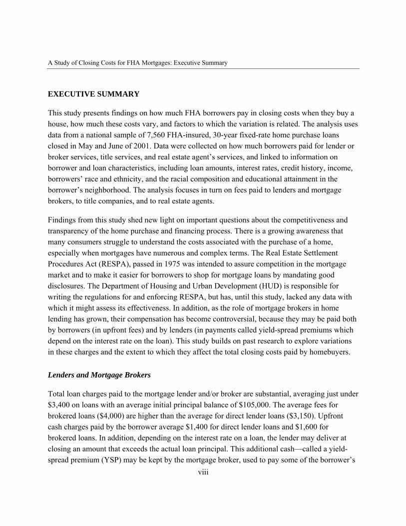
This study presents findings on how much FHA borrowers pay in closing costs when they buy a house, how much these costs vary, and factors to which the variation is related. The analysis uses data from a national sample of 7,560 FHA-insured, 30-year fixed-rate home purchase loans closed in May and June of 2001. Data were collected on how much borrowers paid for lender or broker services, title services, and real estate agent’s services, and linked to information on borrower and loan characteristics, including loan amounts, interest rates, credit history, income, borrowers’ race and ethnicity, and the racial composition and educational attainment in the borrower’s neighborhood. The analysis focuses in turn on fees paid to lenders and mortgage brokers, to title companies, and to real estate agents.
Findings from this study shed new light on important questions about the competitiveness and transparency of the home purchase and financing process. There is a growing awareness that many consumers struggle to understand the costs associated with the purchase of a home, especially when mortgages have numerous and complex terms. The Real Estate Settlement Procedures Act (RESPA), passed in 1975 was intended to assure competition in the mortgage market and to make it easier for borrowers to shop for mortgage loans by mandating good disclosures. The Department of Housing and Urban Development (HUD) is responsible for writing the regulations for and enforcing RESPA, but has, until this study, lacked any data with which it might assess its effectiveness. In addition, as the role of mortgage brokers in home lending has grown, their compensation has become controversial, because they may be paid both by borrowers (in upfront fees) and by lenders (in payments called yield-spread premiums which depend on the interest rate on the loan). This study builds on past research to explore variations in these charges and the extent to which they affect the total closing costs paid by homebuyers.
Lenders and Mortgage Brokers
Total loan charges paid to the mortgage lender and/or broker are substantial, averaging just under $3,400 on loans with an average initial principal balance of $105,000. The average fees for brokered loans ($4,000) are higher than the average for direct lender loans ($3,150). Upfront cash charges paid by the borrower average $1,400 for direct lender loans and $1,600 for brokered loans. In addition, depending on the interest rate on a loan, the lender may deliver at closing an amount that exceeds the actual loan principal. This additional cash—called a yield-spread premium (YSP) may be kept by the mortgage broker, used to pay some of the borrower’s
viii
A Study of Closing Costs for FHA Mortgages: Executive Summary
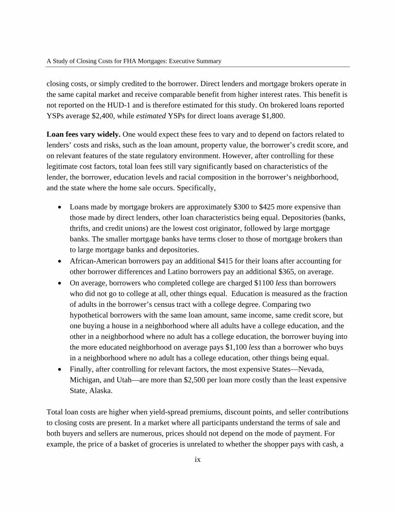
closing costs, or simply credited to the borrower. Direct lenders and mortgage brokers operate in the same capital market and receive comparable benefit from higher interest rates. This benefit is not reported on the HUD-1 and is therefore estimated for this study. On brokered loans reported YSPs average $2,400, while estimated YSPs for direct loans average $1,800.
Loan fees vary widely. One would expect these fees to vary and to depend on factors related to lenders’ costs and risks, such as the loan amount, property value, the borrower’s credit score, and on relevant features of the state regulatory environment. However, after controlling for these legitimate cost factors, total loan fees still vary significantly based on characteristics of the lender, the borrower, education levels and racial composition in the borrower’s neighborhood, and the state where the home sale occurs. Specifically,
• Loans made by mortgage brokers are approximately $300 to $425 more expensive than those made by direct lenders, other loan characteristics being equal. Depositories (banks, thrifts, and credit unions) are the lowest cost originator, followed by large mortgage banks. The smaller mortgage banks have terms closer to those of mortgage brokers than to large mortgage banks and depositories.
• African-American borrowers pay an additional $415 for their loans after accounting for other borrower differences and Latino borrowers pay an additional $365, on average.
• On average, borrowers who completed college are charged $1100 less than borrowers who did not go to college at all, other things equal. Education is measured as the fraction of adults in the borrower’s census tract with a college degree. Comparing two hypothetical borrowers with the same loan amount, same income, same credit score, but one buying a house in a neighborhood where all adults have a college education, and the other in a neighborhood where no adult has a college education, the borrower buying into the more educated neighborhood on average pays $1,100 less than a borrower who buys in a neighborhood where no adult has a college education, other things being equal.
• Finally, after controlling for relevant factors, the most expensive States—Nevada, Michigan, and Utah—are more than $2,500 per loan more costly than the least expensive State, Alaska.
Total loan costs are higher when yield-spread premiums, discount points, and seller contributions to closing costs are present. In a market where all participants understand the terms of sale and both buyers and sellers are numerous, prices should not depend on the mode of payment. For example, the price of a basket of groceries is unrelated to whether the shopper pays with cash, a
ix
A Study of Closing Costs for FHA Mortgages: Executive Summary
credit card, or a check, or whether the seller must make change. In principle, the mortgage market could be equally transparent and competitive. If it were, the data would reveal a clear trade-off between the upfront cash borrowers pay and the interest rates on their loans, where more up-front cash yields a lower rate and vice versa. The present value difference in payments at the higher interest rate should equal the reduction in up-front cash. Borrowers whose loans have a yield-spread premium (reflecting a higher interest rate) should pay less in up-front cash. Borrowers who pay points to reduce their interest rate should have a lower present value of payments approximately equal to the cash points paid. And if the seller contributes to the buyer’s closing costs, the total closing costs should be unaffected.
The data reveal a market that is not even close to this ideal. How far the market is from the ideal varies by type of lender, but no type is close. Yield-spread premiums, discount points, and seller contributions to closing costs are all sources of complexity in a mortgage loan. Borrowers end up with more expensive loans when the terms are more complex:
• Borrowers on average save only $20 in up-front cash for each $100 they pay in yield-spread premium, for a net loss (or extra cost) of $80. Those who borrow through mortgage brokers see a benefit of only $7 per $100, for a net loss of $93, while those who borrow from large mortgage banks see a net loss of $71 on average, with depositories and smaller mortgage banks in between.
• The terms for “discount points” are on average similar, but more diverse among types of originators. Overall, borrowers see a benefit of only $20 for each $100 of points paid, for a net loss of $80. Those who borrow through mortgage brokers see no benefit at all from paying points, either in lower interest rates or in lower fees with other names. Customers of depositories see benefits of roughly $65 per $100 of points paid (for a net loss of $35), while terms from other direct lenders lie between these.
• When sellers contribute to closing costs one would expect borrowers to save $100 themselves for each $100 contributed by the seller. On average, however, borrowers pay $50 less themselves for each $100 that sellers contribute to their closing costs. Again, terms differ by type of lender. For each $100 the seller contributes, borrowers see a benefit of roughly $70 from depositories and large mortgage banks, but closer to $40 when dealing with brokers.
“No-cost” loans cost less. Borrowers who want to avoid up-front cash fees for loan origination can do so with so-called “no-cost” loans. Borrowers who go for no-cost loans simplify their
x
A Study of Closing Costs for FHA Mortgages: Executive Summary
mortgage shopping because they can compare loans on the basis of just the interest rate, liberating themselves from the difficult rate/cash trade-off. Of course, such loans are not really “no-cost;” in principle, they should have higher interest rates than loans on which borrowers pay up-front cash fees and indeed, they do. But all things considered, borrowers with “no-cost” loans effectively pay $1,200 less for loan origination services than borrowers who pay some lender/broker fees in cash.
The “no-cost” loans also reveal a market that looks more competitive in other important ways: Among these loans, there is little relation between the level of education in a borrower’s neighborhood and how much the borrower is charged, and almost no relation to the borrower’s race or the racial characteristics of the borrower’s neighborhood.
The lower prices and absence of relationships between price and either education or race among the no-cost loans suggests that the complexity introduced by loan terms that involve a combination of cash and interest rate, with variations in yield-spread premiums, points, and even seller contributions makes it more difficult for consumers to figure out their total costs and contributes to higher prices and higher fees for lenders and brokers.
Lenders appear to make lower-priced offers to borrowers they expect to be familiar with market terms. Even on FHA-insured loans, lenders suffer some loss when a loan defaults. However, loan approval rates are only slightly related to loan and borrower characteristics known to be related to the likelihood of default. In fact, lenders appear to raise prices rather than reject less promising loans. Nonetheless, differences in default rates are not the source of the large differences seen in pricing. In particular, after accounting for other differences (notably loan amount and credit score), defaults are unrelated to education levels in the borrower’s neighborhood, but total loan prices are substantially lower for borrowers in neighborhoods with high educational attainment than for those in neighborhoods with low education levels (again, neighborhood educational attainment serves as a proxy here for borrowers’ education level, which is not observed directly).
Lenders and brokers are professionals and always know what competitive loan terms are. It appears that they also have views regarding what their customers know. Lenders make lower-priced offers to borrowers in high-education neighborhoods, evidently expecting them to be familiar with competitive market terms, and these offers are accepted with high frequency (only two percent of lender’s offers are on average rejected in neighborhoods where all adults have a college education). In neighborhoods where borrowers may not be so familiar with prevailing
xi
A Study of Closing Costs for FHA Mortgages: Executive Summary
competitive terms, or may be willing to accept worse terms to avoid another application, lenders make higher-priced offers, and some are accepted. Lenders have higher walk-away rates in these neighborhoods (on average 23 percent in neighborhoods where no adults have a college education), but the profit on the loans that are made appears to more than make up for the cost of processing applications approved but not accepted.
Price discrimination of this type does not arise in competitive markets where shoppers are well informed. Even a consumer who is willing to pay a high price (such as a minority borrower who is especially averse to loan rejection) should be able to easily find and get the competitive price in a competitive market. For price discrimination to be possible, there must be some friction— some inhibition to competition such as high transactions costs or search costs or some limitation on information that makes it difficult for one side of the market (borrowers) to see all available prices. The findings reported here suggest that loan complexity itself creates such friction and that improved consumer disclosures could help many borrowers obtain better terms.
Title Services
In addition to loan fees, homebuyers pay substantial amounts at closing for title services. As with lender/broker fees, title fees vary widely in ways that suggest that markets are not fully transparent or competitive, and that many consumers may be paying more than necessary for these services.
Fees for title services vary widely, are related to education and race, and are highest when other closing costs are also high. Total fees paid for title services average $1,200 per loan. Even after controlling for factors that one would expect to contribute to higher fees, considerable unexplained variation remains:
• Borrowers in African-American neighborhoods pay on average an additional $120 for title services and those in Latino census tracts pay an additional $110, as compared to borrowers residing in neighborhoods with no minorities. How much more minorities pay rises with the concentration of minorities in their neighborhoods. As with lender/ broker fees, the differential charges related to education are large: on average borrowers from neighborhoods where all adults have a college degree pay $200 less than those from neighborhoods where none do, other things equal.
• Differences in average title charges (taking loan and borrower characteristics into account) from the lowest-cost state—North Carolina—to the highest cost states—New
xii
A Study of Closing Costs for FHA Mortgages: Executive Summary
York, Texas, California, and New Jersey—is more than $1,000. The type of title insurance regulation adopted by states explains only a small fraction of this variation
• Title charges are higher when fees paid to lenders, brokers, and real estate agents are also high, again controlling for all relevant loan and borrower characteristics. In other words, the same borrowers are being charged above-average fees for multiple components of their closing costs.
Real Estate Agent Services
Real estate agents do not uniformly charge six percent of house value. Among transactions involving a real estate agent, almost half (47 percent) had real estate agent fees below six percent of house value, 29 percent were exactly six percent, and 24 percent were above six percent. One percent had fees above eight percent. In general, real estate agent’s fees are related to both house values and to down payment amounts; for two houses of the same value, the real estate agent’s fees are lower when the buyer has a smaller down payment. In addition, real estate agents’ fees rise with the fraction of adults in a neighborhood who have a college education. And real estate fees are on average $55 lower in Latino neighborhoods, other things equal. However, no other relations to individual or neighborhood race are present in the fees of real estate agents.
Conclusions and Implications
Loan fees, title fees, and real estate agent fees all add significantly to the total closing costs incurred by homebuyers and therefore warrant ongoing scrutiny. By systematically analyzing the costs incurred by a nationally representative sample of 7,560 FHA-insured home purchase borrowers, this study sheds new light on the magnitude and variability of these costs. All three components of closing costs considered here vary with borrower characteristics, lender characteristics, neighborhood racial composition, and across states, even after controlling for factors that are legitimately related to lender costs. Minority borrowers and borrowers in minority neighborhoods and neighborhoods with lower educational attainment consistently pay higher fees, other things being equal. These variations suggest that markets are not fully transparent or competitive.
Complicated loan arrangements raise the total costs to homebuyers and increase the variability of fees, suggesting that lenders and brokers in particular profit when transactions are complex and consumers have a harder time comparing alternatives. Moreover, it appears that lenders and
xiii
A Study of Closing Costs for FHA Mortgages: Executive Summary
mortgage brokers make their most favorable offers to borrowers that they consider knowledgeable about competing alternatives. Borrowers in neighborhoods with low educational attainment receive substantially higher-cost offers, and although a significant share “walk away” from these offers, enough accept them to be profitable to lenders and brokers.
Consumers need more complete and understandable information about all the costs that will be incurred at closing so that they are better able to assess the trade-offs between up-front costs and interest rates and effectively shop and compare the costs of alternative offers.
xiv

A Study of Closing Costs for FHA Mortgages: Part A — Background
PART A: BACKGROUND
Chapter I: Introduction
Motivation and Background
This study analyzes the closing costs and mortgage terms for a nationwide sample of 7,560 FHA-insured, 30-year fixed-rate loans made for the purchase of a house. The study is motivated by several considerations. One is to evaluate the success of the Real Estate Settlement Procedures Act of 1975 (RESPA) and its implementing regulations. The original goal of RESPA was to assure competition in the mortgage market and to make it easier for borrowers to shop for mortgage loans by mandating good disclosures. HUD writes the regulations for and enforces RESPA but has, until this study, lacked any data for studying RESPA’s effectiveness.
A second goal is to study the role of mortgage brokers. As mortgage brokers became an important part of mortgage lending through the 1990s, their compensation became controversial. Brokers may be paid both by borrowers (in up-front cash fees) and by wholesale lenders (in cash payments called yield-spread premiums [YSPs], which depend on the interest rate on the loan). Plaintiffs in litigation charged that YSPs were illegal kickbacks under RESPA. This litigation produced detailed data on closing costs and mortgage terms that had not been studied before, mainly because of the high cost of retrieving and assembling such data. Analysis of the data turned up evidence of wide variations in terms received by borrowers, differential charges by race, even larger differentials by borrower education, and suggestive evidence that simpler loans facilitated more effective mortgage shopping, resulting in better terms for borrowers. These findings question the effectiveness of present mortgage disclosures. One issue on which the litigation did not shed much light is whether borrowers get different terms from brokers versus direct lenders. That issue is addressed in this study.
In addition, there is increasing awareness that many consumers struggle to understand all financial products, not just mortgages, especially those with numerous and complex terms. A growing academic literature focuses on these issues. Federal agencies responsible for disclosure rules and regulations have done little to assess whether consumers understand required disclosures or whether improved disclosures could contribute more to consumers’ understanding.1 This is changing; new research on disclosures is under way, and the potential for
1
A Study of Closing Costs for FHA Mortgages: Part A — Background
disclosures to help financial consumers is coming to be appreciated. One goal of this study is to seek evidence on whether mortgage borrowers might benefit from improved disclosure.
The Data
The analysis here examines the detailed terms on 7,560 FHA-insured loans originated in May and June 2001. All these loans have fixed interest rates and 30-year terms. All loans are for the purchase of a home (no refinancings) by an owner-occupant. The original loan balances average just over $105,000.
The fees paid to lenders and mortgage brokers, real estate agents, and title service companies were collected from the borrowers’ HUD-1 settlement statements. The goal of collecting this information is to study how these charges relate to such borrower and property characteristics as borrower income, credit history, race, loan amount, sex, age, and house value, plus such neighborhood characteristics as income, house values, racial composition, education levels, and loan approval and rejection rates. The analysis focuses on how loan and borrower characteristics relate to how much borrowers are charged.
Data for this study come from various sources. The most important, and the most expensive to collect, is the detailed data on fees paid from each borrower’s HUD-1 settlement statements. In addition, data were collected from the FHA loan files on interest rates, loan amounts, house values, demographic characteristics (age, sex, race, marital status), and credit scores, plus defaults and delinquencies to date. The FHA files also contain borrower addresses, allowing determination of each borrower’s census tract.
From census data it was possible to gather information about neighborhood income levels, house values, racial composition, and educational attainment. The census information was also used to tie in HMDA data on mortgage originations, approvals, and rejections for each borrower’s census tract.
A more detailed discussion of data gathering and sources appears in appendix III.
The Issues
Taking out a mortgage loan is both the largest and most complex financial transaction most households ever undertake. Two features of the transaction make it difficult for borrowers. First
2
A Study of Closing Costs for FHA Mortgages: Part A — Background
is the analytically difficult rate-point trade-off. Borrowers must choose between paying some closing costs in cash at origination or covering these costs over time through a higher interest rate on the loan and thus a higher periodic payment. Or borrowers can pay all closing costs in cash and even pay additional “discount points” in exchange for a lower interest rate on a loan. Most, but not all, FHA borrowers pay some of their lender/broker fees in up-front cash. The idea that the lender must somehow cover the fixed costs of originating a loan and that this can be accomplished with cash now or with a higher interest rate is clear enough. How much cash now should be exchanged for a given change in the interest rate—the rate-point trade-off—is the challenging aspect of the decision.
The second difficulty is the sheer volume of different charges with which the home buyer is confronted and uncertainty about whether each is compulsory, optional, or negotiable. The two main categories of charges are for loan origination and title services (and real estate agent’s services if a real estate agent is used), while smaller categories include mortgage insurance (all FHA loans have FHA mortgage insurance), appraisals, credit reports, tax service, and more. Lenders and mortgage brokers, whose cash fees average about $1,450 a loan in this sample, often break down their own charges into a large number of different fees, each with its own name. Title services, averaging $1,350 a loan here, are also frequently broken down into many different fees. In addition, many other necessary payments are not for settlement services, such as accrued interest on the loan for the first partial month of ownership, various local and regional transaction taxes and fees, contributions to the buyer/owner’s loan escrows for hazard insurance and property taxes on the house, and more.
The result is a bewildering array of different numbers that go into determining the size of the check the buyer must write at closing. Borrowers seldom know the complete total of these charges until a date very close to the loan closing—often only at the closing itself. A recent study by the Federal Trade Commission (Lacko and Pappalardo 2007) that focuses on mortgage disclosure documents (the good faith estimate and the HUD-1 settlement statement) confirms that borrowers are bewildered by mortgage selection.
For data collection, 32 standard categories of fees payable to the lender or broker were created in the data collection template, yet it was still necessary to record thousands of additional charges in extra fields. In principle, lenders could combine all these separate charges in a single fee for origination, but they rarely choose to describe their services in this way.
3
A Study of Closing Costs for FHA Mortgages: Part A — Background
Of the three main categories of settlement services—realty, loan origination, and title services— loan origination is the most difficult analytically. The most complex aspect of loan terms is the trade-off between how much up-front cash the borrower pays versus the interest rate on the loan. Understanding this trade-off is essential to understanding not only the analysis done here but also most previous research in mortgage lending. The next section discusses this trade-off.
Analysis of a Mortgage Rate Sheet
This section illuminates how the rate-point trade-off works from a mortgage lender’s perspective. Some of the loans studied here are made through direct lenders such as depositories and mortgage banks. Others are made through mortgage brokers.2 Mortgage brokers are middlemen. They have relationships with wholesale lenders who give them, daily or even more frequently, the terms on which they are lending. The mortgage broker finds borrowers, offers them a deal, and earns money potentially in two ways: first, as up-front cash fees paid by the borrower to the broker, and second, as a fee paid by the lender that is tied to the rate paid by the borrower. The higher the rate, the higher the broker’s fee from the lender, other things equal. Mortgage brokers and direct lenders deal in the same wholesale market and face similar wholesale market terms.
The mortgage broker is not the borrower’s agent. Mortgage brokers are like any other market seller of shoes or groceries who buys at wholesale and sells at retail. Their goal as profit maximizers is to find the cheapest wholesale terms and charge what the market will bear. Some mortgage brokers may represent themselves as the borrower’s mortgage shopper (“Oh, you don’t need to get any other quotes, I look at terms from twenty-five wholesale lenders every day, you won’t find rates lower than I find.”), but in principle their motivations are the same as those of any other middlemen.
The terms offered by wholesale lenders to mortgage brokers are detailed on a document called a rate sheet. The rate sheet indicates the payment the wholesale lender will make to the mortgage broker for a loan of a given amount at a given interest rate. Because the rate sheets given by wholesale lenders to mortgage brokers make the rate-point trade-off so clear, consider first the mechanics of the terms offered to mortgage brokers by wholesale lenders as represented on their rate sheets.
All lenders, wholesale and retail, face a similar rate-point trade-off dictated by prices set in the secondary mortgage markets. Close to 100 percent of all FHA and VA mortgages are securitized
4

A Study of Closing Costs for FHA Mortgages: Part A — Background
through GNMA soon after origination. GNMA securitizes only new loans, not seasoned loans, giving originators strong incentive to securitize loans promptly. Even a lender who intends to hold a loan will generally securitize it first in order to hold a liquid mortgage-backed security instead of an illiquid “whole loan.” Thus, the pricing in the secondary market feeds back powerfully to the primary market and assures that all lenders face close-to-identical opportunity costs in lending.
Mortgage brokers typically do business with a dozen or so wholesale lenders who stand ready to commit funds, lock in an interest rate, and provide funds for the loan at closing. The wholesale terms on the various rate-point alternatives offered are communicated to mortgage brokers on lender’s rate sheets. Table 1-1 shows a typical rate sheet from a wholesale lender for a day in April 2000, for 30-year, fixed-rate, conventional loans. A rate sheet for FHA loans would not be identical to this one, but it would function identically.
The left-most column, in bold, shows the contract interest rate, or “coupon” rate on the loan, quoted in one-eighth increments or “ticks.” This is the interest rate that will be used to calculate the borrower’s payments. The top line indicates the length of time for which the lender will “lock in” the rate to give the lender and borrower the time needed to assemble the paperwork to complete the loan. If the loan does not close before the lock expires, the borrower may not be able to get that rate if rates generally have moved up. If rates have moved down, the borrower may get a lower rate. The lock is an option to the borrower and an obligation to the lender: the lender must stand ready to fund the loan at that rate regardless of how rates move between the lock date and the expiration of the lock. To provide a lock, brokers (and retail lenders as well) sometimes require an up-front payment of several hundred dollars from the borrower, often in an application fee, sometimes in an explicit lock fee.
5
A Study of Closing Costs for FHA Mortgages: Part A — Background
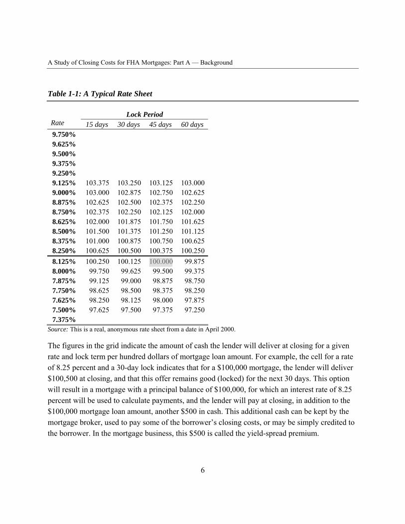
Table 1-1: A Typical Rate Sheet
Rate 15 days Lock Period
30 days 45 days 60 days 9.750% 9.625% 9.500% 9.375% 9.250% 9.125% 103.375 103.250 103.125 103.000 9.000% 103.000 102.875 102.750 102.625 8.875% 102.625 102.500 102.375 102.250 8.750% 102.375 102.250 102.125 102.000 8.625% 102.000 101.875 101.750 101.625 8.500% 101.500 101.375 101.250 101.125 8.375% 101.000 100.875 100.750 100.625 8.250% 100.625 100.500 100.375 100.250
8.000% 99.750 99.625 99.500 99.375 7.875% 99.125 99.000 98.875 98.750 7.750% 98.625 98.500 98.375 98.250 7.625% 98.250 98.125 98.000 97.875 7.500% 97.625 97.500 97.375 97.250 7.375%
8.125% 100.250 100.125 100.000 99.875
Source: This is a real, anonymous rate sheet from a date in April 2000.
The figures in the grid indicate the amount of cash the lender will deliver at closing for a given rate and lock term per hundred dollars of mortgage loan amount. For example, the cell for a rate of 8.25 percent and a 30-day lock indicates that for a $100,000 mortgage, the lender will deliver $100,500 at closing, and that this offer remains good (locked) for the next 30 days. This option will result in a mortgage with a principal balance of $100,000, for which an interest rate of 8.25 percent will be used to calculate payments, and the lender will pay at closing, in addition to the $100,000 mortgage loan amount, another $500 in cash. This additional cash can be kept by the mortgage broker, used to pay some of the borrower’s closing costs, or may be simply credited to the borrower. In the mortgage business, this $500 is called the yield-spread premium.
6
A Study of Closing Costs for FHA Mortgages: Part A — Background
Despite the requirement that the YSP on brokered loans be disclosed on the HUD good faith estimate, often it is not. All lenders, including direct lenders, have a functional equivalent of a yield-spread premium, but only mortgage brokers are required to disclose it.
Considering another cell in the column for a 30-day lock, if the borrower accepts a rate of 8.5 percent, the lender will deliver $101,375 at the closing. By contrast, to get a rate of 7.5 percent on a 30-day lock, the broker arranging a loan of $100,000 will have to pay $2,500 cash at closing—that is, pay 2.5 points (also known as discount points)—at closing, and the broker will likely charge the borrower for at least this amount in addition to origination and other fees.3
For the 45-day lock period, there is an interest rate (in this instance 8.125 percent) for which the lender delivers exactly the mortgage amount at closing and neither requires nor provides additional cash. This is called the par interest rate for the 45-day lock. There is no par rate for the 15-, 30-, or 60-day locks. Because mortgage interest rates are quoted on ticks of 1/8 of a percentage point, frequently no loan will be quoted exactly at par, as one will arise only if the par interest rate happens to fall on a tick. Sometimes it does, often it does not.
Loans with interest rates above par are called premium loans—those on which the lender pays a yield-spread premium. This payment is also sometimes called a “service release premium,” a “broker’s premium,” “lender’s premium,” “deferred premium,” and even “discount rebate.” The terminology used for this payment on HUD-1 settlement statements is far from uniform. Perhaps the term “service release premium” crept in because the typical payment on a premium loan is on the same order of magnitude as the value of the servicing on a loan.4 The term “discount rebate” reflects a little more logic: yield-spread premiums are clearly analogous to yield-spread discounts and are properly thought of as negative points. The borrower can pay points to reduce the interest rate below par, or receive points for accepting an above-par rate. Thus, the YSP can be logically thought of as negative discount points.
In practice, the yield-spread premium is always paid to the broker, not the borrower. Sometimes the borrower’s cash closing costs are lower when she pays an interest rate that results in a yield-spread premium, and sometimes they are not. In one study of all brokered loans, a representative mix of FHA, VA, conventional and jumbo, borrowers’ cash payments to brokers fell about 55 cents for each dollar of YSP (Woodward 2003).
The rate sheet is not the only tool lenders use for pricing. Lenders also have adjustments to the amounts paid to brokers for differentials in borrower credit (positive if the borrower’s credit is
7
A Study of Closing Costs for FHA Mortgages: Part A — Background
better, negative for poorer), for larger loan amounts (lenders pay a premium for larger loan amounts), for the standard of documentation (negative price adjustment for low-documentation or no-escrow loans), and other features.
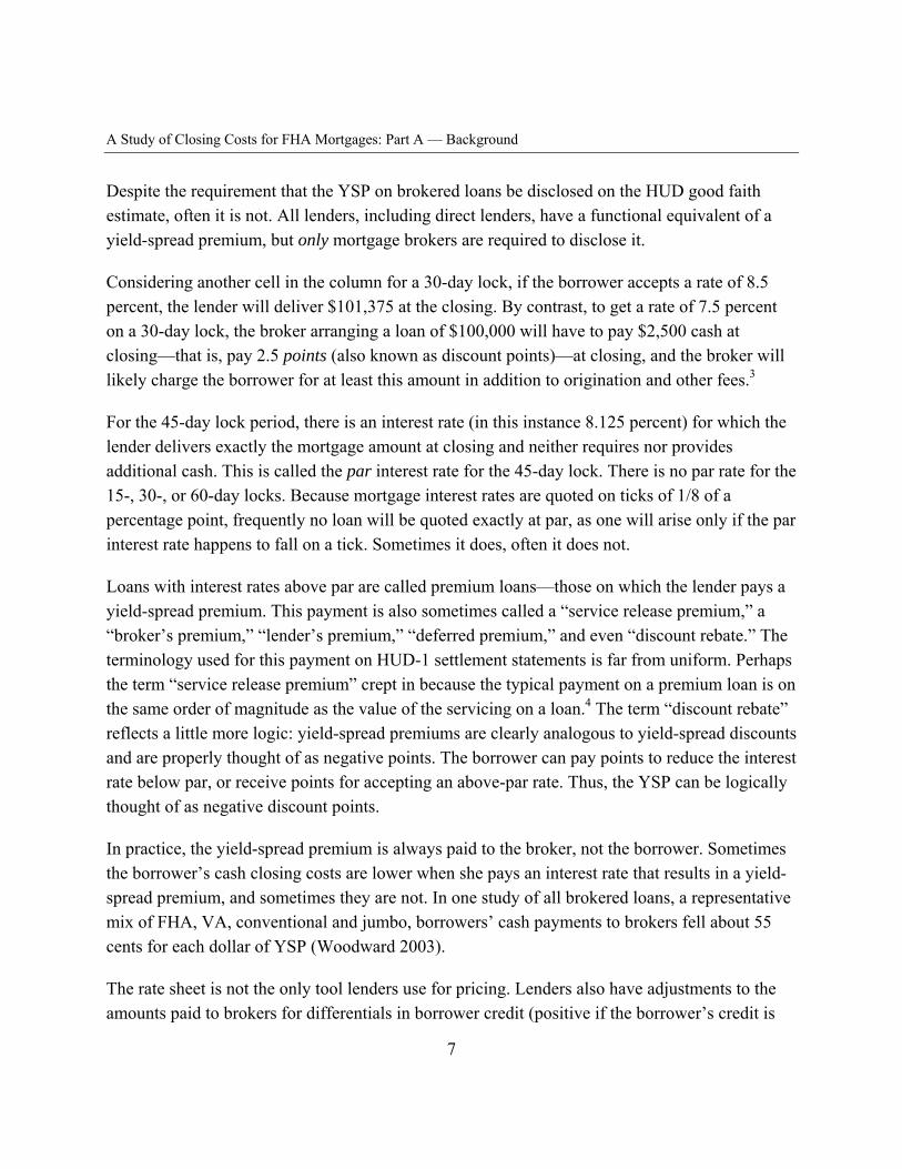
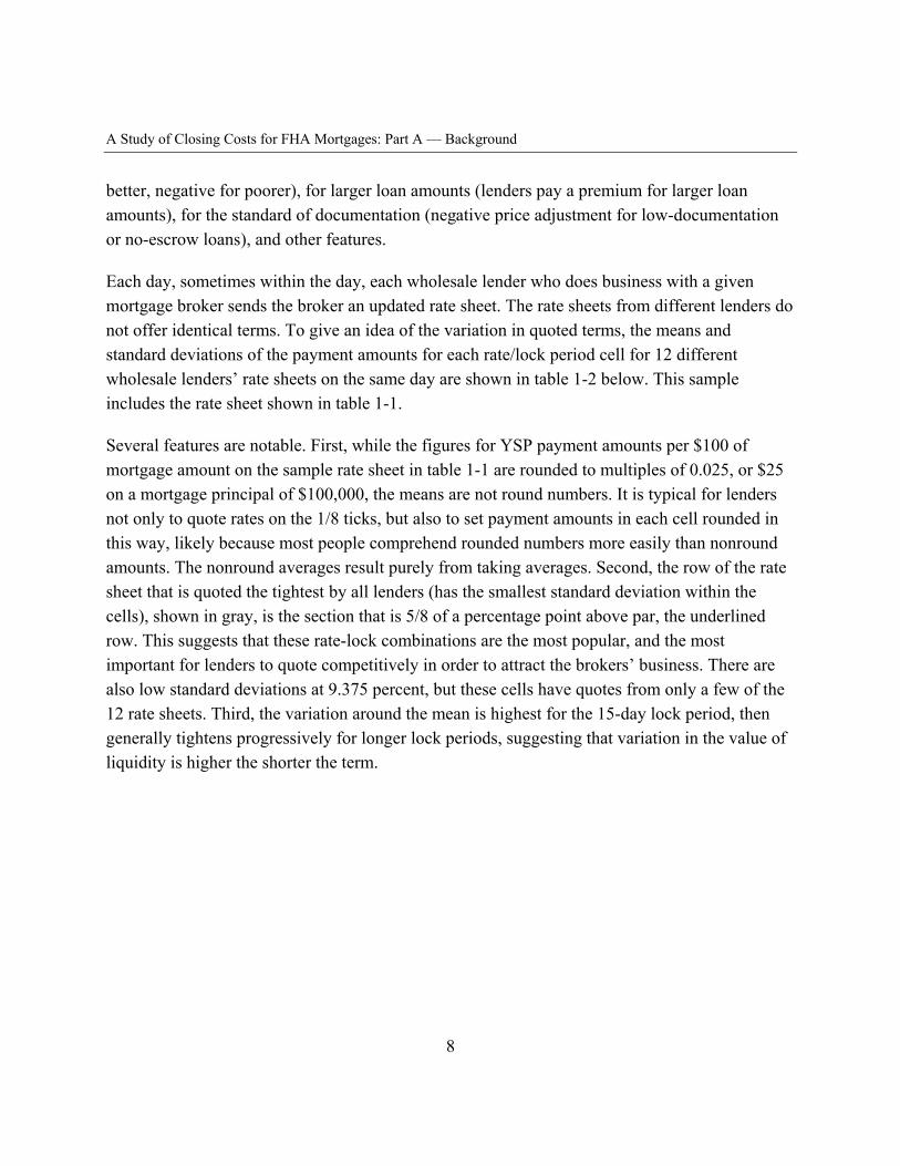
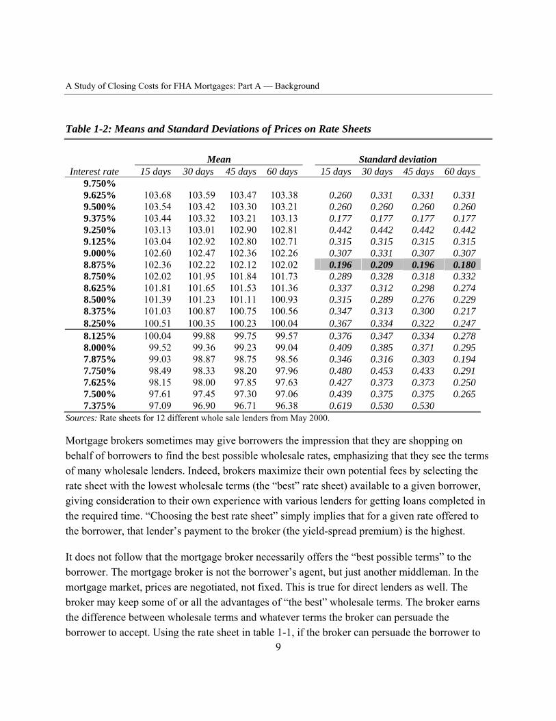
Each day, sometimes within the day, each wholesale lender who does business with a given mortgage broker sends the broker an updated rate sheet. The rate sheets from different lenders do not offer identical terms. To give an idea of the variation in quoted terms, the means and standard deviations of the payment amounts for each rate/lock period cell for 12 different wholesale lenders’ rate sheets on the same day are shown in table 1-2 below. This sample includes the rate sheet shown in table 1-1.
Several features are notable. First, while the figures for YSP payment amounts per $100 of mortgage amount on the sample rate sheet in table 1-1 are rounded to multiples of 0.025, or $25 on a mortgage principal of $100,000, the means are not round numbers. It is typical for lenders not only to quote rates on the 1/8 ticks, but also to set payment amounts in each cell rounded in this way, likely because most people comprehend rounded numbers more easily than nonround amounts. The nonround averages result purely from taking averages. Second, the row of the rate sheet that is quoted the tightest by all lenders (has the smallest standard deviation within the cells), shown in gray, is the section that is 5/8 of a percentage point above par, the underlined row. This suggests that these rate-lock combinations are the most popular, and the most important for lenders to quote competitively in order to attract the brokers’ business. There are also low standard deviations at 9.375 percent, but these cells have quotes from only a few of the 12 rate sheets. Third, the variation around the mean is highest for the 15-day lock period, then generally tightens progressively for longer lock periods, suggesting that variation in the value of liquidity is higher the shorter the term.
8
A Study of Closing Costs for FHA Mortgages: Part A — Background
Table 1-2: Means and Standard Deviations of Prices on Rate Sheets
Mean Standard deviation Interest rate 15 days
9.750% 9.625% 103.68 9.500% 103.54 9.375% 103.44 9.250% 103.13 9.125% 103.04 9.000% 102.60 8.875% 102.36 8.750% 102.02 8.625% 101.81 8.500% 101.39 8.375% 101.03 8.250% 100.51
30 days
103.59 103.42 103.32 103.01 102.92 102.47 102.22 101.95 101.65 101.23 100.87 100.35
45 days
103.47 103.30 103.21 102.90 102.80 102.36 102.12 101.84 101.53 101.11 100.75 100.23
60 days
103.38 103.21 103.13 102.81 102.71 102.26 102.02 101.73 101.36 100.93 100.56 100.04
15 days
0.260 0.260 0.177 0.442 0.315 0.307
30 days
0.331 0.260 0.177 0.442 0.315 0.331
45 days 60 days
0.331 0.260 0.177 0.442 0.315 0.307
0.331 0.260 0.177 0.442 0.315 0.307
0.196 0.209 0.196 0.180 0.289 0.328 0.318 0.332 0.337 0.312 0.298 0.274 0.315 0.289 0.276 0.229 0.347 0.313 0.300 0.217 0.367 0.334 0.322 0.247 0.376 0.347 0.334 0.278 0.409 0.385 0.371 0.295 0.346 0.316 0.303 0.194 0.480 0.453 0.433 0.291 0.427 0.373 0.373 0.250 0.439 0.375 0.375 0.265 0.619 0.530 0.530
8.125% 8.000% 7.875% 7.750% 7.625% 7.500% 7.375%
100.04 99.52 99.03 98.49 98.15 97.61 97.09
99.88 99.36 98.87 98.33 98.00 97.45 96.90
99.75 99.23 98.75 98.20 97.85 97.30 96.71
99.57 99.04 98.56 97.96 97.63 97.06 96.38
Sources: Rate sheets for 12 different whole sale lenders from May 2000.
Mortgage brokers sometimes may give borrowers the impression that they are shopping on behalf of borrowers to find the best possible wholesale rates, emphasizing that they see the terms of many wholesale lenders. Indeed, brokers maximize their own potential fees by selecting the rate sheet with the lowest wholesale terms (the “best” rate sheet) available to a given borrower, giving consideration to their own experience with various lenders for getting loans completed in the required time. “Choosing the best rate sheet” simply implies that for a given rate offered to the borrower, that lender’s payment to the broker (the yield-spread premium) is the highest.
It does not follow that the mortgage broker necessarily offers the “best possible terms” to the borrower. The mortgage broker is not the borrower’s agent, but just another middleman. In the mortgage market, prices are negotiated, not fixed. This is true for direct lenders as well. The broker may keep some of or all the advantages of “the best” wholesale terms. The broker earns the difference between wholesale terms and whatever terms the broker can persuade the borrower to accept. Using the rate sheet in table 1-1, if the broker can persuade the borrower to
9
A Study of Closing Costs for FHA Mortgages: Part A — Background
pay a broker’s fee of $1,000 cash up front and a rate of 8.75 percent with a 60-day lock, the broker makes the $1,000 cash from the borrower plus a YSP payment of $2,000 from the lender for each $100,000 of loan amount. The broker may be willing to perform brokerage services for less than this amount but also may believe the borrower will accept these higher terms, and thus the broker does not necessarily offer the “best possible” terms—what economists would call a reservation price. The only way the borrower can learn that the broker might offer better terms is to gather other offers, threaten to take the business elsewhere, and ask the broker to match or improve them. Some journalists have suggested that by representing themselves as the borrower’s loan shopper, mortgage brokers may discourage borrowers from shopping the loan market themselves.
The incentives faced by mortgage brokers may differ from those of a loan officer for a bank or mortgage bank because of the different structures of their compensation. Traditionally, loan officers are paid a salary, plus some bonus for volume, and in the longer run a bonus for the profitability of their books of loans. Mortgage brokers are freelancers who work on commission only. Their compensation is the difference between the retail terms agreed to by the borrower and the wholesale terms quoted on the rate sheet. As traditional lenders compete more directly with mortgage brokers, the compensation for their agents may be shifting toward that of mortgage brokers. Nonetheless, the results reported below show measurable differences in how brokers versus direct lenders interact with borrowers.
Borrowers generally cannot access brokers’ rate sheets. Brokers’ contracts with wholesale lenders often preclude brokers from showing wholesale rate sheets to borrowers. HUD disclosure rules require only that mortgage brokers disclose the YSP on the loan the borrower is going to receive; they do not require that brokers disclose the YSP on hypothetical alternative loans. Rate sheets make the rate-point trade-off crystal clear to brokers. Borrowers learn the trade-off only from general market information and by getting quotes from multiple originators.
The Logic of “Points”
Why does the mortgage market offer such elaborate arrangements on mortgage loans? Mortgage lending differs from most other kinds of consumer lending in that mortgage loans often have upfront charges. Is this merely a trade-off of cash now for cash later? The trade-off shown on rate sheets suggests that the answer is no. There is more to the rate-point trade-off: the rate at which cash is exchanged for rate adjustments changes as the rate on the loan rises. The changing rate
10
A Study of Closing Costs for FHA Mortgages: Part A — Background
point trade-off reflects the relationship between the value of the option to prepay the mortgage loan and the expected timing of prepayment.
In the United States, residential mortgages are prepayable by the borrower with no or minimal prepayment penalties by state law in all states. When the loan has a fixed interest rate, the option to prepay has considerable value. Even adjustable-rate mortgages (ARMs) have a nontrivial prepayment option value due to the fixed costs of loan origination and to periodic and life-of-loan caps on their interest rates.5 The choice of whether to pay closing costs in cash at origination or with a higher interest rate affects the borrower’s interest rate in two ways. First, when the borrower opts for less cash up front, the lender adjusts the rate upward so the present value of the additional payment amount covers the lender’s up-front costs. Second, the higher the interest rate, the more likely it is that, should interest rates fall, the borrower will prepay her loan and refinance. Thus, as the borrower seeks to cover larger amounts of up-front costs in the interest rate, two forces move the rate upward: first, the rate must rise to capture the costs over time; and second, the higher the rate, the shorter the anticipated life of the loan, so the costs must be recouped in fewer payments. Thus, on every rate sheet the amount of additional cash forthcoming for any upward adjustment in the rate falls as the rate rises.
Why would a borrower ever pay more up-front to get a lower interest rate? Since the goal of taking out a loan in the first place is to spread the cost over many years, why not always choose the option that rolls all the costs into the interest rate? Because of the second force that raises rates as more up-front costs are rolled into the rate—paying for closing costs with a higher rate not only raises the rate in order to absorb these costs, but also raises it further because borrowers with a higher rate are, other things equal, more likely to prepay. This adjustment is symmetric: for the borrower who expects to be in the same house for a while, and thus to not have reason to prepay other than to refinance at a lower rate, paying discount points brings a lower interest rate not only because the borrower has essentially paid some of or all the lender’s fixed costs, but also because the lower rate reduces the likelihood of prepayment, thus increasing the likely life of the loan.6 Borrowers cannot disclaim their option to prepay, but they can make it less valuable, and thus less expensive, by paying points to lower their interest rate (or by choosing an ARM instead of a fixed-rate loan).
The sooner a borrower expects to move, the more likely a loan with a higher interest rate and lower up-front cash is a lower-cost option. In principle, borrowers’ expectations about movements in interest rates should also affect their decisions. But interest rate movements are
11
A Study of Closing Costs for FHA Mortgages: Part A — Background
difficult to predict, especially over longer terms. It is thus difficult to know how much borrower expectations about movements in interest rates ought to, or do, influence their rate-point choices.
Nonetheless, borrowers with only a small down payment, as are most FHA borrowers, are not really in a position to have cash with which to pay points to reduce the interest rates on their loans.
12
A Study of Closing Costs for FHA Mortgages: Part A — Background
Chapter II: Review of Previous Research
There is little previous research specifically on mortgage closing costs, but there is considerable research relevant to this study on such topics as mortgage interest rates, non-real-estate consumer lending, and commodities such as automobiles. The auto and auto lending markets are similar to the mortgage market in that transactions have large dollar values and prices are negotiated. The findings in that body of research can help us interpret the findings of this study.
Research in Mortgage Lending Costs
The only prior existing study of complete mortgage terms (loan rate plus lender/broker up-front charges and other settlement services) is Woodward (2003), which analyzes total compensation to mortgage brokers (cash from the borrower plus the YSP from the lender, which is well-measured from records of the wholesale lender) and total payments to all settlement service providers (broker and lender plus title agent and all other settlement services except for realty services). The findings, based on a mix of 2,600 conventional, jumbo, and FHA loans, originated between 1996 through 2001 by different mortgage brokers but all funded by the same wholesale lender, are as follows:
1. The trade-off between the broker’s up-front cash payments from the borrower and compensation arising from interest-rate adjustments in the form of yield-spread premiums is not what would be expected in a fully transparent market. On average, borrowers’ upfront cash closing costs are lower by about 55 cents for each dollar of YSP paid by the lender to the mortgage broker, other factors equal (including loan amount, credit quality, loan-to-value ratio, lock period, and median area income). The average dollar amount of the YSP for these loans was $1,250, and the average total broker fees were $2,400.
2. Total loan costs (up-front cash plus YSP) vary by the mix of their source. Borrowers who rolled all closing costs into the rate on their loan (presumably from requesting a “no-cost” loan, meaning a loan with no cash paid up front), and thus had all their up-front loan costs, including title services, covered by a YSP, paid total closing costs that were $1,500 lower than those of other borrowers, other things equal. This $1,500 is an economically important fraction of average total closing costs of $4,000. Perhaps borrowers got better terms on no-cost loans because they were able to shop based on rate only, thus avoiding the difficult rate-point evaluation. When borrowers paid their brokers only with a YSP,
13
A Study of Closing Costs for FHA Mortgages: Part A — Background
and no cash, but paid other up-front fees with cash, they paid $670 less to their brokers, other things equal.
3. Loan terms vary with borrower education. Borrowers with BA degrees paid total origination fees of $1,500 less than did borrowers without one, other things equal. This education differential is three times the size of the differential paid by African American borrowers compared to otherwise similar borrowers.
While the findings of Woodward (2003) represent the first analysis of borrower interest rate and all up-front charges together, they confirmed earlier findings from examination of interest rates alone. Courchane and Nickerson (1997) studied the interest rates and points (but not other cash charges) on loans made by retail bank lenders. Direct lenders have internal rate sheets. Some borrowers are quoted a “standard” rate, and some are quoted from other cells with higher interest rates on the rate sheet. When a borrower pays an interest rate higher than the “standard” rate, the difference is called an “overage.” Overages are economically equivalent to yield-spread premiums. Courchane and Nickerson find that minorities on average pay higher overages than do other borrowers. Studying different lenders, Black, Boehm, and DeGennaro (2001a) also find that minorities pay higher overages. Neither of these studies has data on cash fees charged to borrowers, so they are not conclusive regarding whether minorities pay higher loan terms overall. However, the direction of their findings, of worse terms offered to minority borrowers, is confirmed by Woodward (2003), which reckons both rate and up-front fees charged to borrowers.
In another study of loans within a single lender, Steiner (2000) focuses on how sensitive different types of borrowers are to price when choosing the type and size of loan. She estimates the own-price and cross-price elasticity of loan demand by looking at choices across the lender’s different mortgage products. She calculates elasticities using data on rates and closing points without imposing a specified relationship between the two. Steiner finds that with changes in both rates and points, minority borrowers have nearly zero elasticity demand (their choices are very insensitive to price), while white borrowers have very elastic demand (their choices are very sensitive to price), consistent with the patterns of pricing differentials found in the Courchane and Nickerson (1997) and Black and colleagues (2001a) studies.
El Anshasy, Elliehausen, and Shimazaki (2004) study the all-in interest rates (coupon rate plus amortized up-front charges) for data from subprime mortgage lenders. Their data consist only of the all-in rates, and it is not possible to separate the original coupon from amortized cash fees.
14
A Study of Closing Costs for FHA Mortgages: Part A — Background
They conclude that for the loans they study, brokered loans are not more costly than loans originated directly by lenders. El Anshasy and colleagues have a rich array of information about the individual borrowers, including race and educational attainment, as well as neighborhood mobility and density, and they use these data to analyze the borrower choices of brokers versus banks as originators. They do no analyze the relationship between race or education and what borrowers pay for their loans.
Another relevant study showing the importance of factors other than standard default risk characteristics in mortgage outcomes is a survey of how borrowers become prime versus subprime borrowers done for Freddie Mac by Courchane, Surette, and Zorn (2003). This study does not have detailed data on mortgage terms, but it has many insights about how borrowers with credit that would qualify them for a prime loan end up as subprime borrowers. This study finds that the standard risk characteristics (credit scores, assets, loan-to-value ratio) explain much of the difference in what type of loan borrowers get. More can be explained, however, by including such factors as shopping behavior (do borrowers search for best rates or lowest monthly payments? Are they familiar with mortgage market terms?), adverse life events (divorce, illness, unemployment, large drop in income), channel (borrowers using brokers are more likely to get subprime loans than those who use lenders, other things equal), and age (older borrowers are more likely to have subprime loans, other things equal). After taking account of these factors, race had little influence on whether borrowers had subprime loans.
Stango and Zinman (2006), studying data from the Survey of Consumer Finances, have two interesting findings relevant to this study. First, they document that consumers tend to underestimate the interest rate implied by a given loan amount and payment schedule, and that this downward bias becomes smaller as borrower education, income, and assets rise. They suggest that this vulnerability to underestimate the interest rate may explain why lenders have historically marketed loans emphasizing monthly payments while hiding or distorting interest rates. Second, Stango and Zinman find that consumers who borrow from banks (and thrifts and credit unions) pay no price for their bias, while those who borrow from non-bank finance companies (upon whom the hand of the Truth in Lending Act rests more lightly because they are not regulated as banks) pay 300 to 400 basis points more than bank borrowers.
Another important finding is that minority borrowers’ loan applications are rejected more often than are the applications of white borrowers. This has been established in many studies and is not disputed. Instead, in this literature (reviewed by LaCour-Little 1999), the dispute concerns whether minorities are treated unfairly. The literature is not conclusive.
15
A Study of Closing Costs for FHA Mortgages: Part A — Background
Research on Defaults, Prepayment Rates, and Discrimination
Gary Becker (1957) suggested that the ultimate test of discrimination (in the sense of differential treatment of some customers for whom the seller has a distaste, such as in the case of racial discrimination) is whether the discriminated-against customers are, in the limited accounting sense, more profitable customers. He argued that if there was truly discrimination, sellers would be willing to deal with distasteful customers only at a higher price; thus, evaluated simply on the basis of money profit (which would not include the personal and subjective “cost” of dealing with the distasteful customers), these customers should be the more profitable. In the context of mortgage lending, the qualification of profitability “based on expected value” needs to be added. If lenders charge minority borrowers more but also experience higher default or prepayment losses on minority loans, whether Becker-type discrimination is present will turn on the differences in charges versus differences in the additional expected costs.
Loan profitability depends on the original loan terms plus the eventual loan delinquencies, defaults and prepayments. A loan that defaults seldom returns all the money lent; a loan that prepays when interest rates have fallen limits the lender’s gain and may result in a loss. Minorities differ from white borrowers in their default and prepayment behaviors. Two studies of FHA experience, find that borrowers living in neighborhoods with higher fractions of African Americans have higher default rates than other borrowers, other things equal (Cotterman 2004). This is also true in the loans studied here. The most thorough study of defaults and prepayments together is by Deng and Gabriel (2004), who find that for FHA loans originated between 1992 and 1996, minorities have higher loan default rates, but they prepay their loans less aggressively, on average. Zorn and Van Order (2001) have a similar finding for the conventional mortgage market. On net, these two studies covering similar periods find that loans made to minorities gave lenders a risk-return trade-off that is more profitable, not less, than that of white borrowers.
Before concluding that minority loans are more profitable for lenders as a general proposition, consider that default rates for all loans in 1992–96 were unusually low. This was a period of falling interest rates, unusually stable house prices, and relatively low fluctuations in overall economic activity. This period may not be representative of the long-run experience for mortgage lending.
The only studies with clear results on race differences in the profitability of mortgage loan terms to sellers are those of auto loan broker fees by Cohen (2006) (discussed in more detail below) and mortgage loan broker fees by Woodward (2003), both of which find that loan brokers (but
16
A Study of Closing Costs for FHA Mortgages: Part A — Background
not necessarily lenders) earn higher fees on minority loans after accounting for loan amount, credit quality, and other factors. The reason these studies are conclusive while the others are not is because studies looking at subsequent defaults and prepayments must tie original terms to what the lender expected. Cohen (2005) and Woodward (2003) suffer no such limitation: the broker got exactly what was expected (the deal that was made) with no exposure to subsequent events such as defaults or prepayments. Indeed, these two studies find very similar dollar differences: on mortgage loans and on auto loans, African American borrowers pay the loan broker roughly $500 more than do other borrowers, despite the mortgage loans being about five times the size of the auto loans.
It thus appears that by Becker’s profitability test, auto loan brokers and mortgage loan brokers do discriminate because their loans made to minority borrowers are more profitable than their loans made to nonminorities. Nonetheless, it appears that the phenomenon found in Woodward (2003) and Cohen (2005) is not what Becker had in mind as discrimination. Becker imagines a market where sellers prefer not to interact with some types of customers. There are clues that the source of discrimination in these loan markets is not seller distaste for some customers, but lower elasticity of demand—more versus less price sensitivity—on the part of some customers. As a result of their less-elastic demand (lower sensitivity to price), some customers are offered, and accept, higher prices in this negotiated market. If the group getting the higher price gets the worse deal because of lower demand elasticity and consequent price discrimination, this differs from them being distasteful customers. In principle, the inelastic-demand minorities should be more desired customers, and more eagerly sought out by the price-searching mortgage providers. Perhaps using the right measure of search costs (in which lenders and brokers expend more searching for minority borrowers), these loans would not be more profitable.
There is at least one good reason for minorities to be less-aggressive price seekers and thus less-elastic demanders than nonminorities: their loan rejection rates are higher. Given the higher rejection rates, it is easy to imagine that minorities would be more likely than other borrowers to accept any given terms when credit is offered. If the party making the offer is sensitive to this difference, this knowledge can affect the offered terms. In this setting, the technical term “lower price elasticity” masks the basic emotion leading minorities to be offered and to accept worse deals, which is their fear of continuing to search, reapplying, and being rejected.
17
A Study of Closing Costs for FHA Mortgages: Part A — Background
Findings from the Auto Loan Market
The institutional arrangements of the market for auto loans closely parallel those of the home mortgage market. Car buyers can get a loan from their local bank or credit union, or they can arrange financing at the point of sale with the auto dealer who sells them a car. The loan broker, who may be a separate individual within a dealer’s facility, operates with a rate sheet very similar to the rate sheet of the mortgage broker, but simpler. The loans are made immediately, so there is no lock period. On the other hand, car lenders make finer distinctions on credit quality than do mortgage lenders. The car loan rate sheets generally have five credit quality categories, with lower rates for better credit. The rate sheet specifies the amount the wholesale lender will pay the car dealer for each dollar of loan amount at different rates. As with the mortgage rate sheet, the lender pays the car agency more for making loans at higher rates, and this amount is analogous to a yield-spread premium. Cohen (2005) reports that on average, minority car buyers/borrowers agree to higher rates that result in additional payment from the wholesale lender to the car dealer of about $500 per loan on new cars averaging $25,000 in value.
One feature of the auto loan market not found in the mortgage market is that wholesale auto lenders put a ceiling on the upward adjustment of interest rate for the two highest credit-quality buckets, but not for the lower-quality buckets. Cohen (2005) finds that to evade these caps, auto loan brokers sometimes moved borrowers to a lower-quality credit bucket than they merited (based on their credit scores) to quote them higher rates, which were sometimes accepted by the car buyers. Similar limitations are not imposed by wholesale mortgage lenders on the premium that mortgage brokers may quote to borrowers. This study does not attempt to address the question why such caps are seen for car loans, but not mortgage loans, but the question is a good one.
Research Outside Lending
Beyond mortgage lending, considerable research can help interpret the findings in this study. In particular, the research on the terms for cars, which are sold in markets where price is negotiated, is relevant. The relevant facts and principles found in this work, discussed in more detail below, are as follows:
1. Education, income, comparison shopping, and tolerance for engaging in negotiation all have a measurable impact on the eventual price consumers pay in markets for large purchases, such as automobiles.
18
A Study of Closing Costs for FHA Mortgages: Part A — Background
2. Minorities and women pay more for cars than do other consumers. Much of the difference, but not all, is related to education, income, and the willingness to comparison shop and negotiate.
3. Consumers capture a smaller share of the potential gains from trade when they do not know a potential surplus is there.
The Importance of Shopping Behavior
In 1995, Ayres and Siegelman published their findings that minorities and women pay more for new cars than do white men. The role of shopping strategy in these differentials has been investigated by Scott Morton, Zettelmeyer, and Silva-Risso (2005). They find that such factors as knowledge of dealer invoice price, visits to additional dealers, patience, and taste or distaste for bargaining and shopping influence how much consumers pay. The best deals arise from a combination of market knowledge and willingness to negotiate. Stango and Zinman (2006) find that borrowers who are more confused about the relationship between loan amount, payments, and interest rates are less likely to comparison shop for loans.
In another study, Scott Morton, Zettelmeyer, and Silva-Risso (2003) examine auto purchases on and off the Internet. Offline, women pay 0.5 percent more and minorities an extra two percent ($500 again), compared to white men, for equivalent cars. Sixty percent of this price differential for in-person shopping is explainable with such factors as income, education, already having a car (making search costs lower), and willingness to shop (or at least no distaste for shopping). For online car purchases, where customers also negotiate price, there are no race or gender differences in car prices.
Aguiar and Hurst (2005) demonstrate the general importance of shopping and comparing prices, even in markets with posted prices, in their study of expenditure, consumption, and time spent shopping. This study was motivated by the well-documented decline in household expenditures at retirement and the seeming contradiction of this finding with the permanent income hypothesis. Aguiar and Hurst find that the decline in expenditures is only part of the story. At retirement, households spend more time shopping and find better prices, and they spend more time preparing food. Overall, neither the quantity nor quality of consumption declines at retirement.
19
A Study of Closing Costs for FHA Mortgages: Part A — Background
Ian Ayres, in his book Pervasive Prejudice? (2001), explores four possible explanations for why minorities and women pay more for cars. The first two are Becker-type discrimination, involving a seller’s dislike of the buyer. Ayres leans against these sources of differential treatment because auto dealerships hire substantial numbers of minority salespeople and some dealerships are minority-owned but nonetheless behave like other dealerships. He then considers the possibility that minority buyers might have more distaste for bargaining or be more inelastic demanders because they have less knowledge of market prices. The Scott Morton, Zettelmeyer, and Silva-Risso studies confirm both less market knowledge and a distaste for bargaining as sources of differential pricing.
Fully Informed versus Partially Informed Markets
The game-theoretic literature suggests that in bilateral negotiations, the party with less information will generally get a smaller share of the benefit of the bargain. Yet another study of the auto market by Busse, Silva-Risso, and Zettelmeyer (2006) documents the importance of this in two different auto sales promotions. In one promotion, auto manufacturers offer car buyers a $1,000 cash rebate when they buy one of the manufacturer’s cars. In another, they offer $1,000 to dealers who sell such a car. Parallel to the well-known theorem in price theory that the impact of a tax should be the same regardless of whether it is imposed on buyers or sellers, standard economic analysis suggests that the two different promotions should have identical impacts on price paid and the number of cars sold.
The different promotions have very different results in price and sale quantity. When the buyers collect the rebate, both buyer and car salesman know of the promotion. When the sellers get the bonus, only the seller, not the car buyer, knows of its existence. When car buyers get the rebate, consumers get 70 to 90 percent of the benefit of it (their total price including the rebate is about $700–$900 lower than with no promotion). When dealers get the rebate, consumer benefit is only 30 to 40 percent of the surplus amount. The promotions direct to consumers sold more cars than the relatively concealed promotions to salespeople only.
The parallel between the auto dealer promotions and the mortgage market is that lender payments to brokers are well understood by the mortgage brokers but perhaps not by consumers. But the parallel is not perfect. An important difference is that the yield-spread premium is not a temporary promotion by lenders, but a permanent part of how lenders distribute their wholesale
20
A Study of Closing Costs for FHA Mortgages: Part A — Background
terms to mortgage brokers. Despite the permanence of the wholesale arrangements, it seems that few consumers understand them.
Perhaps the most important piece of research on how informed borrowers are in the mortgage market is the Federal Trade Commission’s 2007 report on mortgage disclosure by James Lacko and Janis Pappalardo. It is among the first pieces of federal research to address the adequacy of present disclosures. From in-depth interviews and quantitative testing of recent mortgage borrowers, Lacko and Pappalardo found that current mortgage disclosures fail to convey key mortgage costs to consumers. Using prototype revised disclosures, they established that improved disclosures are feasible. Their testing indicates that the improved disclosures provided the greatest benefit for more complex loans, whose terms presented the most difficulty to both prime and subprime borrowers. They do not have data to evaluate how much this confusion costs borrowers. This issue is addressed in the present study.
21

A Study of Closing Costs for FHA Mortgages: Part B — Lender and Broker Charges
PART B: LENDER AND BROKER CHARGES
Chapter III: A Descriptive Approach to Lender/Broker Charges
Loan Origination Fees
This chapter looks descriptively at the data for the variables of primary interest in this study: charges paid in cash to lenders and brokers (up-front cash), yield-spread premiums, total charges paid by borrowers (up-front cash plus yield-spread premium), coupon rates, and loan amounts.
This descriptive examination is restricted to loans that are clearly not subsidized and have coupon rates above seven percent. Loans in the sample are designated as subsidized if they have contributions to closing costs or down payments by state or local programs, interest rates at or below six percent, or interest rates off the 1/8 tick that is standard in the FHA market. Loans off the 1/8 tick may have been funded through a municipal bond issue. There are 1,433 loans that are clearly not subsidized and report a YSP. Loans with a reported YSP are presumed to be originated by mortgage brokers. Of these, 1,174 have coupon rates above seven percent. Loans with coupon rates above seven percent closed during this period are almost certainly premium loans and would have positive YSPs.
On rate sheets, there is a clear relationship between the YSP and the coupon rate on the loan. For a given loan amount, YSP rises as coupon rate rises. This relationship is also present in the YSPs and coupon rates for the loans with reported YSPs in this study. Figure 3-1 shows a plot of coupon rate against YSP (divided by loan amount) for the 1,174 nonsubsidized loans with reported YSPs and coupon rates above seven percent in this study. Note that the coupon rates cluster on 1/8 ticks.
22
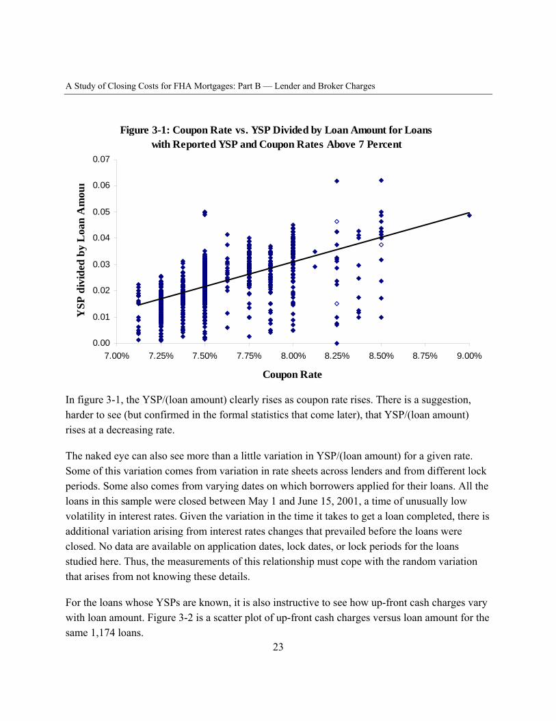
A Study of Closing Costs for FHA Mortgages: Part B — Lender and Broker Charges
23
Figure 3-1: Coupon Rate vs. YSP Divided by Loan Amount for Loans with Reported YSP and Coupon Rates Above 7 Percent
0.00
0.01
0.02
0.03
0.04
0.05
0.06
0.07
7.00% 7.25% 7.50% 7.75% 8.00% 8.25% 8.50% 8.75% 9.00%
Coupon Rate
YSP
div
ided
by
Loa
n A
mou
n
In figure 3-1, the YSP/(loan amount) clearly rises as coupon rate rises. There is a suggestion, harder to see (but confirmed in the formal statistics that come later), that YSP/(loan amount) rises at a decreasing rate.
The naked eye can also see more than a little variation in YSP/(loan amount) for a given rate. Some of this variation comes from variation in rate sheets across lenders and from different lock periods. Some also comes from varying dates on which borrowers applied for their loans. All the loans in this sample were closed between May 1 and June 15, 2001, a time of unusually low volatility in interest rates. Given the variation in the time it takes to get a loan completed, there is additional variation arising from interest rates changes that prevailed before the loans were closed. No data are available on application dates, lock dates, or lock periods for the loans studied here. Thus, the measurements of this relationship must cope with the random variation that arises from not knowing these details.
For the loans whose YSPs are known, it is also instructive to see how up-front cash charges vary with loan amount. Figure 3-2 is a scatter plot of up-front cash charges versus loan amount for the same 1,174 loans.
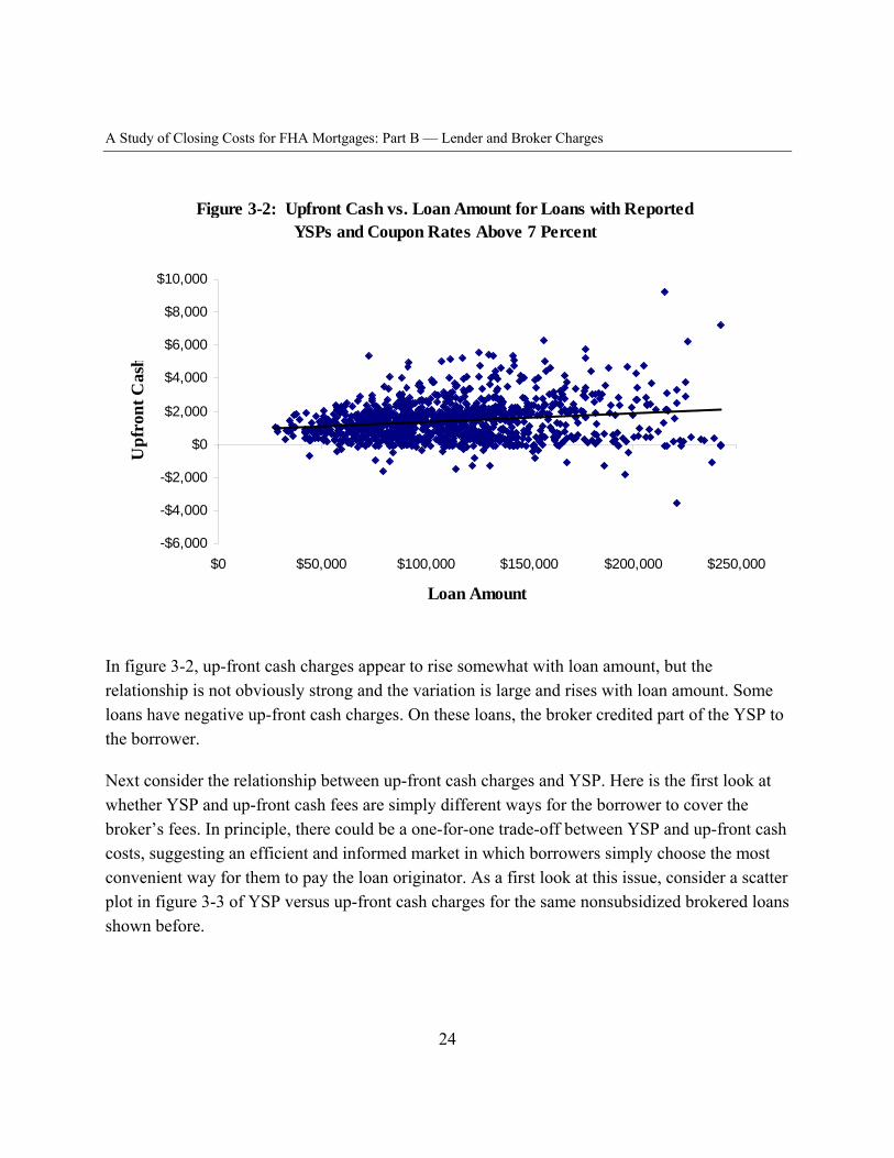
A Study of Closing Costs for FHA Mortgages: Part B — Lender and Broker Charges
24
Figure 3-2: Upfront Cash vs. Loan Amount for Loans with Reported YSPs and Coupon Rates Above 7 Percent
-$6,000
-$4,000
-$2,000
$0
$2,000
$4,000
$6,000
$8,000
$10,000
$0 $50,000 $100,000 $150,000 $200,000 $250,000
Loan Amount
Upf
ront
Cas
h
In figure 3-2, up-front cash charges appear to rise somewhat with loan amount, but the relationship is not obviously strong and the variation is large and rises with loan amount. Some loans have negative up-front cash charges. On these loans, the broker credited part of the YSP to the borrower.
Next consider the relationship between up-front cash charges and YSP. Here is the first look at whether YSP and up-front cash fees are simply different ways for the borrower to cover the broker’s fees. In principle, there could be a one-for-one trade-off between YSP and up-front cash costs, suggesting an efficient and informed market in which borrowers simply choose the most convenient way for them to pay the loan originator. As a first look at this issue, consider a scatter plot in figure 3-3 of YSP versus up-front cash charges for the same nonsubsidized brokered loans shown before.
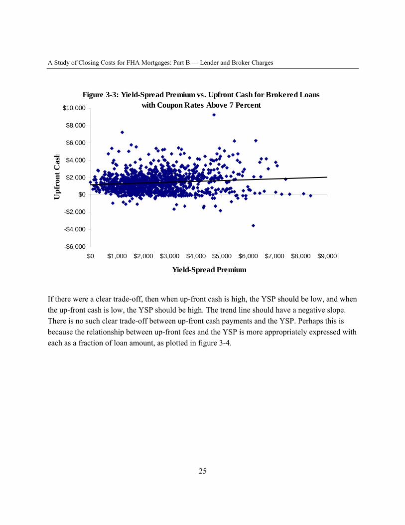
A Study of Closing Costs for FHA Mortgages: Part B — Lender and Broker Charges
25
Figure 3-3: Yield-Spread Premium vs. Upfront Cash for Brokered Loans with Coupon Rates Above 7 Percent
-$6,000
-$4,000
-$2,000
$0
$2,000
$4,000
$6,000
$8,000
$10,000
$0 $1,000 $2,000 $3,000 $4,000 $5,000 $6,000 $7,000 $8,000 $9,000
Yield-Spread Premium
Upf
ront
Cas
h
If there were a clear trade-off, then when up-front cash is high, the YSP should be low, and when the up-front cash is low, the YSP should be high. The trend line should have a negative slope. There is no such clear trade-off between up-front cash payments and the YSP. Perhaps this is because the relationship between up-front fees and the YSP is more appropriately expressed with each as a fraction of loan amount, as plotted in figure 3-4.
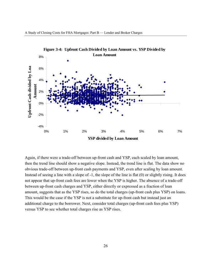
A Study of Closing Costs for FHA Mortgages: Part B — Lender and Broker Charges
26
Figure 3-4: Upfront Cash Divided by Loan Amount vs. YSP Divided by Loan Amount
-4%
-2%
0%
2%
4%
6%
8%
0% 1% 2% 3% 4% 5% 6% 7%
YSP divided by Loan Amount
Upf
ront
Cas
h di
vide
d by
Loa
nA
mou
nt
Again, if there were a trade-off between up-front cash and YSP, each scaled by loan amount, then the trend line should show a negative slope. Instead, the trend line is flat. The data show no obvious trade-off between up-front cash payments and YSP, even after scaling by loan amount. Instead of seeing a line with a slope of -1, the slope of the line is flat (0) or slightly rising. It does not appear that up-front cash fees are lower when the YSP is higher. The absence of a trade-off between up-front cash charges and YSP, either directly or expressed as a fraction of loan amount, suggests that as the YSP rises, so do the total charges (up-front cash plus YSP) on loans. This would be the case if the YSP is not a substitute for up-front cash but instead just an additional charge to the borrower. Next, consider total charges (up-front cash fees plus YSP) versus YSP to see whether total charges rise as YSP rises.
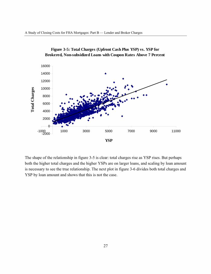
A Study of Closing Costs for FHA Mortgages: Part B — Lender and Broker Charges
27
Figure 3-5: Total Charges (Upfront Cash Plus YSP) vs. YSP for Brokered, Non-subsidized Loans with Coupon Rates Above 7 Percent
-2000
0
2000
4000
6000
8000
10000
12000
14000
16000
-1000 1000 3000 5000 7000 9000 11000
YSP
Tot
al C
harg
es
The shape of the relationship in figure 3-5 is clear: total charges rise as YSP rises. But perhaps both the higher total charges and the higher YSPs are on larger loans, and scaling by loan amount is necessary to see the true relationship. The next plot in figure 3-6 divides both total charges and YSP by loan amount and shows that this is not the case.
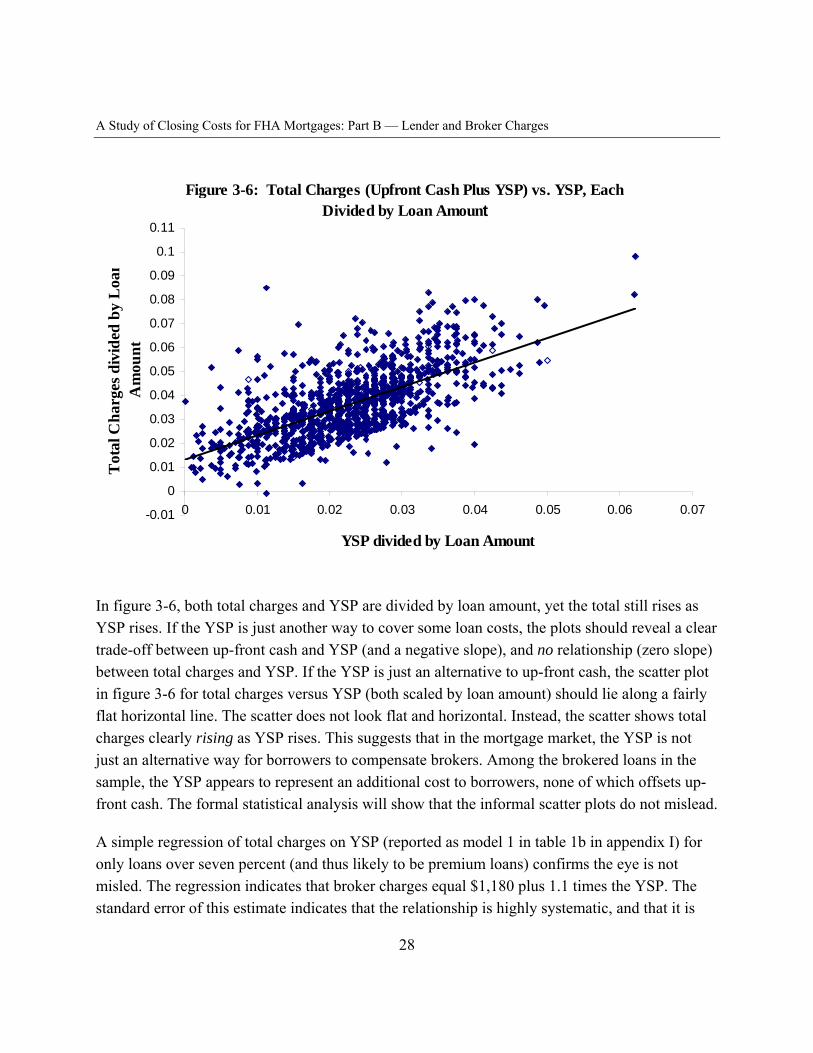
A Study of Closing Costs for FHA Mortgages: Part B — Lender and Broker Charges
28
Figure 3-6: Total Charges (Upfront Cash Plus YSP) vs. YSP, Each Divided by Loan Amount
-0.01
0
0.01
0.02
0.03
0.04
0.05
0.06
0.07
0.08
0.09
0.1
0.11
0 0.01 0.02 0.03 0.04 0.05 0.06 0.07
YSP divided by Loan Amount
Tot
al C
harg
es d
ivid
ed b
y L
oan
Am
ount
In figure 3-6, both total charges and YSP are divided by loan amount, yet the total still rises as YSP rises. If the YSP is just another way to cover some loan costs, the plots should reveal a clear trade-off between up-front cash and YSP (and a negative slope), and no relationship (zero slope) between total charges and YSP. If the YSP is just an alternative to up-front cash, the scatter plot in figure 3-6 for total charges versus YSP (both scaled by loan amount) should lie along a fairly flat horizontal line. The scatter does not look flat and horizontal. Instead, the scatter shows total charges clearly rising as YSP rises. This suggests that in the mortgage market, the YSP is not just an alternative way for borrowers to compensate brokers. Among the brokered loans in the sample, the YSP appears to represent an additional cost to borrowers, none of which offsets up-front cash. The formal statistical analysis will show that the informal scatter plots do not mislead.
A simple regression of total charges on YSP (reported as model 1 in table 1b in appendix I) for only loans over seven percent (and thus likely to be premium loans) confirms the eye is not misled. The regression indicates that broker charges equal $1,180 plus 1.1 times the YSP. The standard error of this estimate indicates that the relationship is highly systematic, and that it is
A Study of Closing Costs for FHA Mortgages: Part B — Lender and Broker Charges
extremely remote that the true slope of the line is far from 1.1, or outside the range from 1.04 to1.16. By this simple analysis, FHA borrowers appear to get essentially no benefit from YSPs on brokered loans with coupon rates above seven percent. Dividing both total charges and YSP by loan amount, the regression (reported as model 2 in table 1b in appendix I) yields a coefficient on YSP of 1.01 (again, precisely estimated, so this is not a fluke), again indicating that all the YSP represents additional compensation to the broker, not a relief from up-front cash fees for the borrower. These same regressions are reported for all nonsubsidized loans as models 1 and 2 in table 1a in appendix I.
Further analysis incorporating other loan and borrower characteristics, reported and discussed at length in coming chapters, will indicate that when FHA borrowers spend a dollar paying a YSP, they save only a few pennies of up-front charges, on net a substantial loss. They get somewhat more up-front cash savings from direct lenders, but not a lot more, far shy of even 50 cents per dollar of YSP.
If the relationships among YSP, total charges, and up-front cash clearly suggest that borrowers get little benefit from higher interest rates (and the attendant YSPs), is this relationship similarly obvious in up-front cash and interest rates also? It is, as shown in the scatter plot in figure 3-7.
29
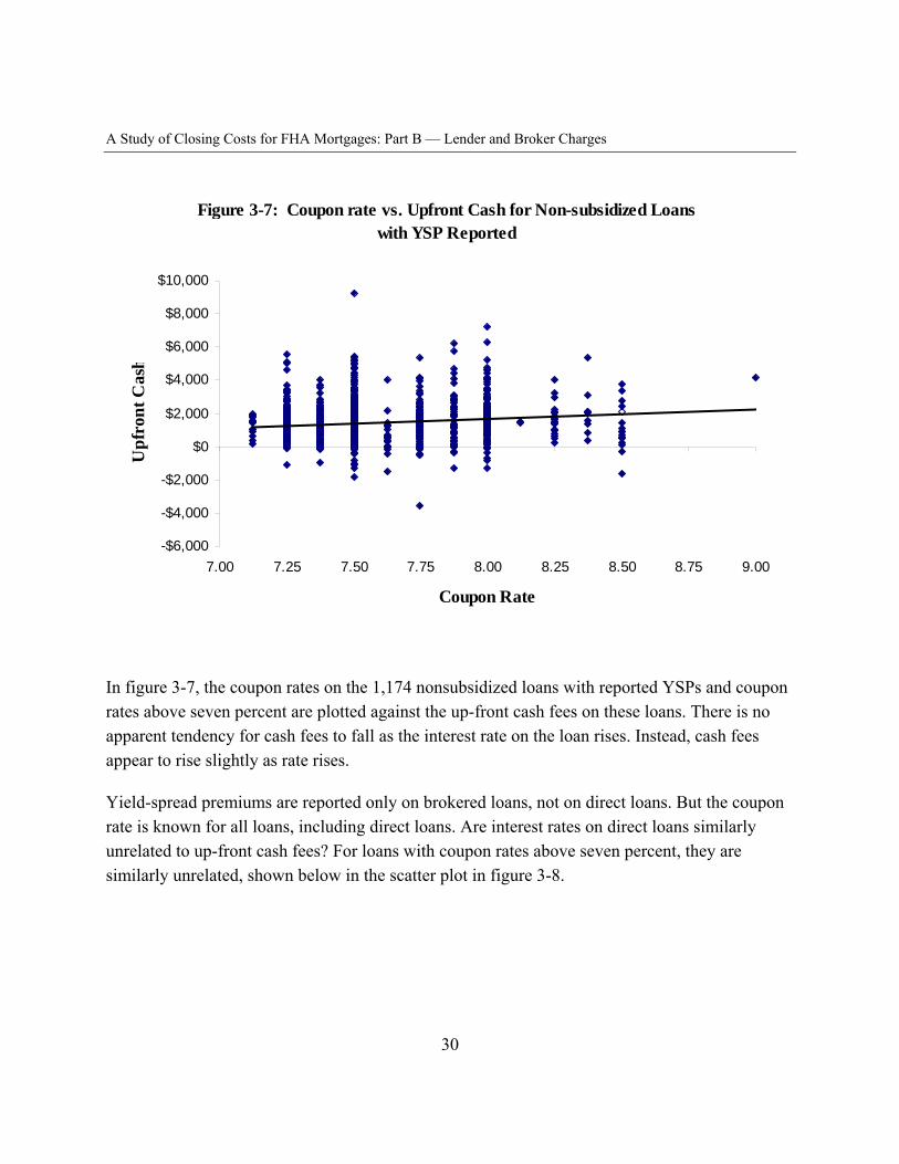
A Study of Closing Costs for FHA Mortgages: Part B — Lender and Broker Charges
30
Figure 3-7: Coupon rate vs. Upfront Cash for Non-subsidized Loans with YSP Reported
-$6,000
-$4,000
-$2,000
$0
$2,000
$4,000
$6,000
$8,000
$10,000
7.00 7.25 7.50 7.75 8.00 8.25 8.50 8.75 9.00
Coupon Rate
Upf
ront
Cas
h
In figure 3-7, the coupon rates on the 1,174 nonsubsidized loans with reported YSPs and coupon rates above seven percent are plotted against the up-front cash fees on these loans. There is no apparent tendency for cash fees to fall as the interest rate on the loan rises. Instead, cash fees appear to rise slightly as rate rises.
Yield-spread premiums are reported only on brokered loans, not on direct loans. But the coupon rate is known for all loans, including direct loans. Are interest rates on direct loans similarly unrelated to up-front cash fees? For loans with coupon rates above seven percent, they are similarly unrelated, shown below in the scatter plot in figure 3-8.
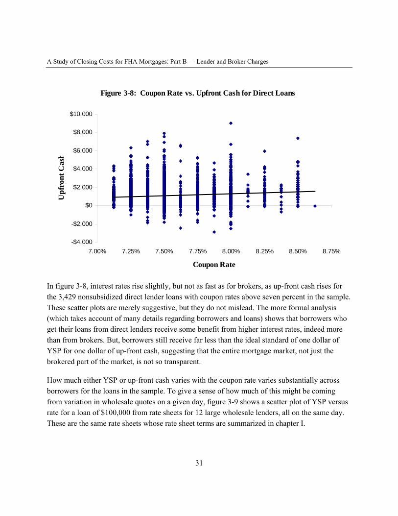
A Study of Closing Costs for FHA Mortgages: Part B — Lender and Broker Charges
31
Figure 3-8: Coupon Rate vs. Upfront Cash for Direct Loans
-$4,000
-$2,000
$0
$2,000
$4,000
$6,000
$8,000
$10,000
7.00% 7.25% 7.50% 7.75% 8.00% 8.25% 8.50% 8.75%
Coupon Rate
Upf
ront
Cas
h
In figure 3-8, interest rates rise slightly, but not as fast as for brokers, as up-front cash rises for the 3,429 nonsubsidized direct lender loans with coupon rates above seven percent in the sample. These scatter plots are merely suggestive, but they do not mislead. The more formal analysis (which takes account of many details regarding borrowers and loans) shows that borrowers who get their loans from direct lenders receive some benefit from higher interest rates, indeed more than from brokers. But, borrowers still receive far less than the ideal standard of one dollar of YSP for one dollar of up-front cash, suggesting that the entire mortgage market, not just the brokered part of the market, is not so transparent.
How much either YSP or up-front cash varies with the coupon rate varies substantially across borrowers for the loans in the sample. To give a sense of how much of this might be coming from variation in wholesale quotes on a given day, figure 3-9 shows a scatter plot of YSP versus rate for a loan of $100,000 from rate sheets for 12 large wholesale lenders, all on the same day. These are the same rate sheets whose rate sheet terms are summarized in chapter I.
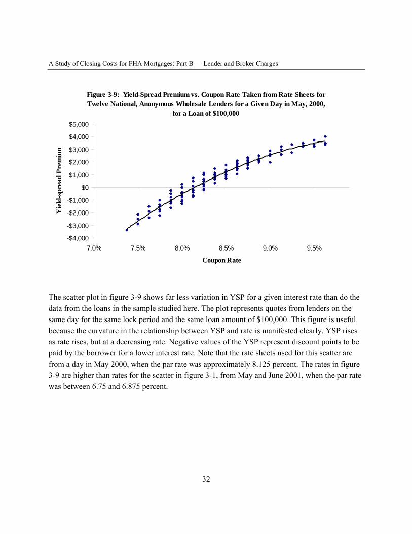
A Study of Closing Costs for FHA Mortgages: Part B — Lender and Broker Charges
Figure 3-9: Yield-Spread Premium vs. Coupon Rate Taken from Rate Sheets for Twelve National, Anonymous Wholesale Lenders for a Given Day in May, 2000,
for a Loan of $100,000
Yie
ld-s
prea
d Pr
emiu
m
$5,000
$4,000
$3,000
$2,000
$1,000
$0
-$1,000
-$2,000
-$3,000
-$4,000
7.0% 7.5% 8.0% 8.5% 9.0% 9.5%
Coupon Rate
The scatter plot in figure 3-9 shows far less variation in YSP for a given interest rate than do the data from the loans in the sample studied here. The plot represents quotes from lenders on the same day for the same lock period and the same loan amount of $100,000. This figure is useful because the curvature in the relationship between YSP and rate is manifested clearly. YSP rises as rate rises, but at a decreasing rate. Negative values of the YSP represent discount points to be paid by the borrower for a lower interest rate. Note that the rate sheets used for this scatter are from a day in May 2000, when the par rate was approximately 8.125 percent. The rates in figure 3-9 are higher than rates for the scatter in figure 3-1, from May and June 2001, when the par rate was between 6.75 and 6.875 percent.
32
A Study of Closing Costs for FHA Mortgages: Part B — Lender and Broker Charges
Chapter IV: Econometric Issues
Constructing a Single Metric of Loan Cost
Terms on brokered loans and direct loans vary in both up-front cash and coupon rate. An analysis of how charges to borrowers vary with loan and borrower characteristics is simplified by putting the terms on the loan into a single metric. The single metric could be an interest rate or it could be a cash amount. For brokered loans, the yield-spread premium converts rate differences into cash differences, which can be added to up-front cash charges, producing such a single metric. Something similar is needed to put all lenders’ terms into a single metric so comparisons in terms can be made by loan and borrower characteristics.
The principles of the relationship between YSP and coupon rate are clear from the rate sheets. Because all mortgage originators participate in the same capital market, the principles apply with equal force to direct lenders and brokers. At any point in time all lenders face essentially the same cost of funds. However, because direct lenders, who take title of the loan at least for a short period, are not required by HUD’s RESPA regulations to report yield spread premiums (on the conceit that the YSP cannot be determined at settlement), they do not report YSPs. Nonetheless, at least 3,100 direct-lender loans in the sample have interest rates sufficiently high that, had they been made by brokers, they would unquestionably have positive YSPs. To compare terms for brokered and direct loans, estimated YSPs are needed for the direct lenders.
In principle, two routes to a single metric are possible, one via rate, and another via cash. To use the rate approach, one would need to estimate how long a loan will be outstanding, amortize the up-front cash fees over that period, divide by loan amount, and add this amount to the borrower’s coupon rate. The alternative is to put the interest differential into cash terms—essentially what the YSP does for brokered loans—and add this cash amount to the borrower’s up-front cash fees. The superiority of the YSP (cash) approach lies in how it addresses the uncertainty regarding the life of the loan. The rate sheets implicitly embed the market’s views as to how long loans at different coupon rates will remain outstanding. Thus, by using the YSP to map out the relationship between rate and expected present-value-difference in cost, the analyst relies on the market’s view of how long loans will live and does not have to estimate it herself.
33

A Study of Closing Costs for FHA Mortgages: Part B — Lender and Broker Charges
Estimating YSPs
Using this second approach requires a measure of the YSP for all the loans in the sample. The loans on which YSP is reported can be used to estimate the relationship between rate and YSP per dollar of loan amount, and thus to calculate a YSP for the loans not reporting a YSP. The problem with this approach is that mortgage brokers are only required to report YSPs if the YSP is positive. In principle there could be brokered loans with negative YSPs in the sample, but such loans could not be identified as brokered loans. Given this limitation, two approaches were considered.
1. Estimate the relationship between rate and YSP using only YSPs on loans with coupon rates above seven percent. Loans with rates above seven percent at the time the sample was drawn are very likely to have had positive YSPs. Use this relationship to calculate estimated YSPs for all loans, and use all nonsubsidized loans for the analysis.
This approach has the advantage that the interest rate adjustment (per dollar of loan amount) is the same for all loans at the same coupon rate. The possible problem with this approach is that if there are any below-par brokered loans, it is not possible to identify them. Based on the data from Woodward (2003), it is unlikely that there are very many below-par brokered loans.
2, As above, use only YSPs on loans with coupon rates above seven percent to measure the YSP-rate relationship and use the estimated relationship to calculate estimated YSPs for all loans. However, instead of using all unsubsidized loans, use only loans with rates above seven percent for the analysis, discarding the rest of the data.
This approach has several merits. First, the interest rate adjustment per dollar of loan amount is the same for all included loans at the same rate. Second, this approach uses YSP data for all loans with rates above seven percent to infer YSP only for loans with rates above seven percent; it does not infer YSPs for loans with rates outside this range. The substantial disadvantage of this approach is that it discards considerable information—the terms on loans with lower coupon rates. The distribution (cumulative distribution function) of rates on loans with no YSP reported (presumed to be direct loans because no YSP is reported) lies almost strictly below that for loans with YSP reported. For loans with coupon rates above seven percent, the distribution of rates for loans without YSP lies strictly below the distribution of rates for loans with YSP reported. Because loans originated during this time period and carrying rates below 7 percent were unlikely to pay a YSP if originated in a brokered transaction, they are less likely to be accurately
34
A Study of Closing Costs for FHA Mortgages: Part B — Lender and Broker Charges
identified as direct or brokered loans based on YSP reporting. If direct loans are truly cheaper than brokered loans, restricting the analysis only to loans above a given rate may make direct and brokered loans look more alike than they truly are.
The solution used here is to report the analysis for both sets of data: all nonsubsidized loans (the first approach to YSP), and only nonsubsidized loans with coupon rates above seven percent (the second approach to YSP), where the data’s distinction between broker and direct lender loans is more reliable.
The general shape of the study findings is not very different for these two approaches. Using only the loans with rates above seven percent slightly reduces differences between brokers and direct lenders, as expected, but it also reduces the measured benefit to borrowers for both brokered and direct loans coming from YSPs, discount points, and seller contributions to closing costs. In other words, the brokered loans and direct loans are more similar among the loans with coupon rates above seven percent, but the entire group looks more exploitive of borrowers.
One more measurement (econometric) issue deserves discussion: whether to use actual YSPs or estimated YSPs on the brokered loans for the analysis. In principle, for both approaches 1 and 2, the actual YSPs on brokered loans with coupon rates above seven percent could be used for calculating total charges and for analyzing how total charges vary with YSP. Using actual versus estimated YSPs as part of total lender/broker charges, the variable of interest in most of the analysis, should make little difference in the measured coefficients. Table 19 in appendix I provides estimates done both ways to demonstrate that not only in theory, but in practice, the measures are similar.
However, when the YSP is used as an explanatory (or right-hand) variable, as it is in the analysis in chapter VI (where borrower loss from the YSP is measured), using an estimated YSP instead of an actual can, in principle, bias downward the measurement of the relation of YSP to total charges and make the benefit look larger than it truly is. Because estimated YSPs must be used for direct loans, estimated YSPs are also used for brokered loans so the comparison is “apples to apples.” Thus, the benefit of the YSP is likely overstated for both groups. The sensitivity of the results to estimated versus actual YSPs is shown in tables 19 through 22 of appendix I, and gives an idea of how large the bias may be. Table 19 shows that how total charges are related to loan and borrower characteristics varies little depending on whether actual or estimated YSPs are used for the brokered loans. Table 20 shows that the measure of how much more expensive brokered loans are, using a dummy variable, is nearly identical ($415 versus $422) for actual
35
A Study of Closing Costs for FHA Mortgages: Part B — Lender and Broker Charges
versus estimated YSPs. Table 21 shows that when analyzing all nonsubsidized brokered loans, the measure of borrower loss from the YSP ($93 per $100 of YSP paid) is nearly identical using actual versus estimated YSPs. Finally, table 22 shows that analyzing only the brokered loans with coupons over seven percent, the coefficient measuring borrower loss from the YSP is higher using estimated YSPs than actual YSPs, but not a great deal higher. Indeed, no important question addressed in this study (Are brokered loans more expensive than direct loans? Do borrowers benefit from the YSP? How are total charges related to borrower race or education? and more) has a different answer using estimated versus actual YSPs for the brokered loans.
Treatment of Subsidized Loans
Subsidized loans are not included in this analysis of total loan charges, either for estimating YSPs or for analyzing how loan terms relate to borrower and loan characteristics or for analyzing title charges. The subsidized loans are included in the analysis of fees to real estate agents because it appears that these fees are not subsidized. Loans were designated as subsidized if they had contributions from state or local programs to closing costs or down payments, had coupon rates at or below six percent, or had coupon rates that were off the 1/8 tick standard in the mortgage market, and thus possibly funded through some state or local bond issue. A total of 1,194 loans were categorized as subsidized, leaving 6,366 nonsubsidized loans with reliable data for all relevant fields, of which 1,433 had a YSP reported, and thus are presumed to be brokered loans.
Model for Estimating Yield-Spread Premiums
The wholesale relationship between YSP and rate is clear from an examination of the rate sheets. As coupon rate rises, the YSP as a fraction of loan amount also rises, but it rises at a decreasing rate. This suggests a quadratic specification, such as
YSP/(loan amount) = β0 + β1(coupon rate) + β2(coupon rate)2
with a negative coefficient expected on the term where rate is squared. To isolate the YSP as the dependent variable, multiply through by loan amount:
YSP = β0 *(loan amount) + β1(coupon rate)* (loan amount) + β2(coupon rate)2*(loan amount)
36
A Study of Closing Costs for FHA Mortgages: Part B — Lender and Broker Charges
Only loans with coupon rates above seven percent and reported YSPs were used to measure this relationship.
The results of this estimation are reported in model 1 in table 2 in appendix I.
Estimating Credit Scores
A second preliminary step to the full analysis is to estimate credit scores for the 420 loans lacking credit scores. Incorporating estimated credit scores makes it is possible to measure the impact of credit scores on loan terms and, at the same time, the impact of lacking a credit score. The 6,007 nonsubsidized loans with credit scores are used to measure the relationship of credit score to other nonsubjective borrower characteristics. The regression used to measure this relationship is shown in model 1 in table 3 in appendix I. In addition, the basic specification relating charges to loan and borrower characteristics is reported in models 2 and 4 in table 4a and 4b in appendix I estimated two different ways, first using all loans including those with estimated credit scores (model 2), and second using only loans with reported credit scores (model 4). The main impact of using estimated credit scores is to enable measurement of the additional cost to borrowers who lack credit scores. The variation in other coefficients is within a single standard error.
Bootstrapped Standard Errors
All standard errors are computed by bootstrap instead of ordinary least squares standard errors. The main reason for using bootstrapped standard errors is that some variables, such as the metropolitan area income, census tract–level educational attainment and tract racial composition, are observed at the census tract or metropolitan area level. To compensate for clustering on these values (which means that many observations have the same value because they are in the same census tract or metropolitan area, which by its nature reduces variation), the standard errors are computed by bootstrap. A bootstrap measurement takes many (400) random samples (with replacement) of census tracts and their loans from the data, computes the regression coefficients, and then computes standard errors of the coefficients as the standard deviation of each coefficient across the different regression estimates.
Perhaps of greater importance, because YSPs are estimated, regression models that involve YSPs are computed using a bootstrap estimator that accounts for predicting YSP and for estimating the relationship between charges and loan and borrower characteristics.
37
A Study of Closing Costs for FHA Mortgages: Part B — Lender and Broker Charges
Using bootstrap methods to calculate standard errors does not change the estimated coefficients from what ordinary least squares produces. It accounts for the use of predicted yield-spread premium and for any potential clustering bias in the standard errors. The bootstrapped standard errors can, in principle, be either larger or smaller than OLS standard errors. For this study, all findings that appeared important economically and statistically using OLS are also important economically and statistically using bootstrap.
Remaining Econometric Issues
It is possible that there are loan and borrower characteristics that are systematically related to how much borrowers pay for settlement services that are not included in this study. For example, in Woodward 2003, how much borrowers paid their brokers is related to the length of the term for which the loan was locked. Shorter lock periods are associated with higher fees to brokers. It is not a terribly important variable for explaining the variation in how much borrowers pay, but it is related. In this study, no data were available on when loans were locked or for what term they were locked; when such a variable is excluded, its relationship with the dependent variable will be reflected in the coefficients of the included variables with which it is correlated. There well may be other factors that are important to understanding how loans are priced that are not considered here.
Another issue is how to interpret the coefficients of the regression models. Coefficients calculated with Ordinary Least Squares are unbiased measures of the true relationship between the dependent (left-hand-side) variable and the independent (right-hand-side) variables only if the independent variables are not related to the unobserved error terms in the equation. For example, suppose that borrowers with larger loans also tend to have higher credit scores. If this is the case, then simply regressing how much borrowers are charged on loan amount will generally produce a measure of how much charges rise with loan amount that is too low because an unobserved (or in this case, un-included) variable, credit score, is correlated with how much an individual borrower’s charges depart from the usual relationship between charges and loan amount. Including the credit score as well as loan amount as independent variables will produce a better measure, one in which inclusion of credit score eliminates a source of correlation between the loan amount and the error term.
Should the estimates here be interpreted as causal, in the sense that larger loan amounts “cause” higher borrower charges or status as a minority “causes” higher charges? No, they should not.
38
A Study of Closing Costs for FHA Mortgages: Part B — Lender and Broker Charges
The goal here is to seek relationships, not to identify causality. The data cannot tell us why minorities pay more, nor can it tell us why people from neighborhoods where adults have been in school longer pay less. The data can reject a few hypotheses (such as default rates and dry hole costs) as reasons why the charges are different, but only by establishing that there are no relationships in the data consistent with these hypotheses.
39
A Study of Closing Costs for FHA Mortgages: Part B — Lender and Broker Charges
Chapter V: Loan Origination Fees in Relation to Loan and Borrower Characteristics
This chapter begins with a summary of loan and borrower characteristics. This summary establishes that settlement costs are a substantial burden of buying a home. For the non-subsidized FHA borrowers studied here, total lender/broker charges are about $3,400, the third-party charges (appraisal, credit report, flood certification and tax services) total another $500, and total title charges average $1,350, for total loan-related service charges of roughly $5,250. This figure is more than double the average borrower’s down payment of $2,550. For transactions involving a real estate agent, the agent’s fees add another $6,000. Thus, charges for all settlement services, including services of a real estate agent, total about $11,000 for the sample of unsubsidized FHA loans, which average about $110,000 in loan amount.
To what loan and borrower characteristics are loan charges related? This chapter focuses on the total loan-related charges to borrowers from brokers and lenders. The characteristics examined are
1. the amount of the loan; 2. the median value of owner-occupied houses in the borrower’s census tract; 3. the borrower’s actual or estimated credit score multiplied by loan amount1; 4. a categorical (dummy) variable indicating whether the borrower has a credit score; 5. payment coverage (borrower’s FHA income category, divided by loan amount); 6. median income in the borrower’s metropolitan area, or county for non-metro areas; 7. a categorical variable to indicate whether borrower is African American; 8. a categorical variable to indicate whether borrower is Latino; 9. the fraction of residents in the borrower’s census tract who are African American,
multiplied by loan amount; 10. the fraction of residents in the borrower’s census tract who are Latino, multiplied by loan
amount; and 11. the fraction of adults in the borrower’s census tract who have completed college.
The variables are chosen presuming that the market for mortgage lending is competitive—that is, there are numerous suppliers and entry as a supplier is relatively low cost. Despite this competition, some pricing is likely not competitive (in the sense that price does not equal marginal cost) because of the frictions discussed in chapter II. Thus, two forces likely influence
40
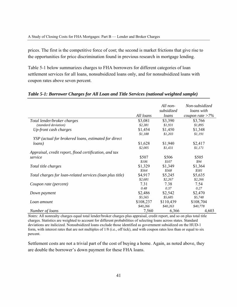
A Study of Closing Costs for FHA Mortgages: Part B — Lender and Broker Charges
prices. The first is the competitive force of cost; the second is market frictions that give rise to the opportunities for price discrimination found in previous research in mortgage lending.
Table 5-1 below summarizes charges to FHA borrowers for different categories of loan settlement services for all loans, nonsubsidized loans only, and for nonsubsidized loans with coupon rates above seven percent.
Table 5-1: Borrower Charges for All Loan and Title Services (national weighted sample)
Total lender/broker charges (standard deviation)
Up-front cash charges
YSP (actual for brokered loans, estimated for direct loans)
Appraisal, credit report, flood certification, and tax service
Total title charges
Total charges for loan-related services (loan plus title)
Coupon rate (percent)
Down payment
Loan amount
Number of loans
All non- Non-subsidized subsidized loans with
All loans loans coupon rate >7% $3,081 $3,390 $3,766 $2,381 $1,931 $1,895
$1,454 $1,450 $1,348 $1,188 $1,203 $1,191
$1,628 $1,940 $2,417 $2,005 $1,431 $1,171
$507 $506 $505 $106 $107 $94
$1,329 $1,349 $1,364 $564 $568 $581
$4,917 $5,245 $5,635 $2,681 $2,267 $2,266 7.31 7.38 7.54 0.48 0.37 0.27
$2,486 $2,542 $2,470 $5,565 $5,685 $5,748
$108,237 $110,439 $108,704 $40,266 $40,263 $40,778
7,560 6,366 4,603 Notes: All nonrealty charges equal total lender/broker charges plus appraisal, credit report, and so on plus total title charges. Statistics are weighted to account for different probabilities of selecting loans across states. Standard deviations are italicized. Nonsubsidized loans exclude those identified as government subsidized on the HUD-1 form, with interest rates that are not multiples of 1/8 (i.e., off tick), and with coupon rates less than or equal to six percent.
Settlement costs are not a trivial part of the cost of buying a home. Again, as noted above, they are double the borrower’s down payment for these FHA loans.
41
A Study of Closing Costs for FHA Mortgages: Part B — Lender and Broker Charges
The most important source of dollar cost differences across borrowers is the dollar amount of the loan. Lenders have higher dollar opportunity costs and higher absolute base-rate expected default costs on larger loans.
Next is variation in cost arising from variation in default risk. Defaults are costly to lenders, even in the FHA market, because FHA reimburses lenders for most of, but not all, the costs of delinquency (which precedes default) and default. Default cost is proportional to the amount loaned, so all factors that may be related to default likelihood are multiplied by loan amount.
A large body of research in mortgage finance (reviewed in chapter II) finds systematic differences in default rates related to loan amount (larger loans are less likely to default), credit history, loan-to-value ratio, and borrower race. Actual defaults for this set of FHA loans are examined later in detail in chapter VIII, and the analysis confirms and refines the relation of defaults to these loan and borrower attributes and some others. Notably, for African Americans, higher default rates are associated with higher neighborhood racial concentration but not with the race of individual borrowers. In addition, after taking account of credit history, loan amount, and race, education at the census tract level is not related to default likelihoods.
A variable important in other studies but omitted from the measurements here is loan-to-value ratio. It is omitted because these are all purchase loans, the average down payments are small, and the loans exhibit so little variation that it is not possible to detect any influence on loan pricing or defaults from loan-to-value ratio.
Another potential cost to the lender is the cost of personnel, which varies with wage levels in different cities. To reflect lender differences in wage costs, median area income is included as a measure of area wage levels. This variable is systematically related to broker charges but has little relation to charges of direct lenders.
The second market force on prices informing the choice of variables is market frictions that give rise to differential pricing based on such borrower attributes as gender, race, and education, as were found in the auto market. The mortgage market meets the criteria that used to be the standard for the presumption of a fully competitive market: numerous sellers and low entry costs. In a competitive market, it is expected that price will equal marginal cost and prices to customers presenting similar levels of cost (especially expected defaults) will be the same. Yet in the studies reviewed in chapter II, there is ample evidence that for automobiles, auto loans, and mortgage loans, females pay more than males, and minorities pay more than nonminorities.
42
A Study of Closing Costs for FHA Mortgages: Part B — Lender and Broker Charges
Such differentials especially appear in markets where price is negotiated, such as automobiles and lending. The auto shopping studies found that customers who have a better idea of what the competitive price is (either because they researched price or sought more offers) are more likely to pay a low price.
Basic Findings
With respect to mortgage lending, total charges, up-front cash plus the yield-spread premium, are strongly related to loan amount in every analysis undertaken in this study. For all nonsubsidized loans, total loan charges rise about $50 for each additional $1,000 of loan amount. Total charges are also related to housing values in the borrower’s census tract, and rise about $2 for each additional $1,000 of average house value in the borrowers’ neighborhood (census tract). For just the loans with coupon rates greater than seven percent, charges have a similar relation to loan amount, but rise $3 instead of $2 for each additional $1,000 of average value in the census tract.
Charges also show a strong relationship to borrower credit scores multiplied by loan amount and fall roughly $440 for each additional 100 points of credit score on a loan for $100,000 (and more for larger loans) for all nonsubsidized loans, and $385 for loans with coupons over seven percent. Borrowers lacking a credit score are charged roughly an additional $325, on average, for both groups. This charge might be related to additional paperwork to verify credit worthiness for borrowers lacking credit scores, or higher expected defaults, but may also reflect price discrimination against less financially savvy borrowers. The data do not admit discerning which of these explanations is the more compelling. Measurements for these findings appear in model 2 in tables 4a and 4b in appendix I.
Total charges are higher in locations where median area income is higher. This relationship is stronger for brokered loans than for direct loans. There are also strong measurable influences from borrower race, both at the individual and neighborhood levels, discussed more fully below.
Including a measure of education differences across borrowers, here reckoned as the fraction of adults in the borrower’s census tract who completed college, was originally motivated by the possibility that education differences might offer some insight into the differences by race. Two important things were learned from the analysis of education. First, including education at the census tract level in the analysis makes little difference in the measures of how different racial groups are treated. The magnitude of the race differentials is not much lowered or raised by incorporating education in the analysis. Second, education is itself even more important than race
43
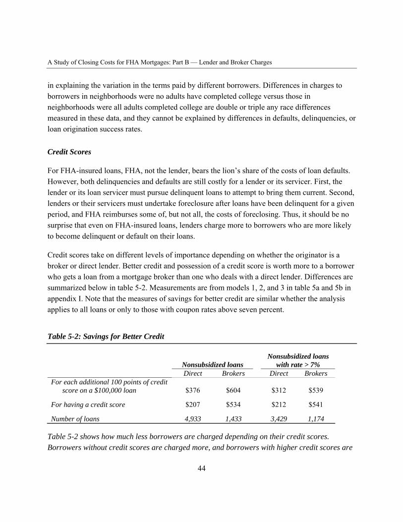
A Study of Closing Costs for FHA Mortgages: Part B — Lender and Broker Charges
in explaining the variation in the terms paid by different borrowers. Differences in charges to borrowers in neighborhoods were no adults have completed college versus those in neighborhoods were all adults completed college are double or triple any race differences measured in these data, and they cannot be explained by differences in defaults, delinquencies, or loan origination success rates.
Credit Scores
For FHA-insured loans, FHA, not the lender, bears the lion’s share of the costs of loan defaults. However, both delinquencies and defaults are still costly for a lender or its servicer. First, the lender or its loan servicer must pursue delinquent loans to attempt to bring them current. Second, lenders or their servicers must undertake foreclosure after loans have been delinquent for a given period, and FHA reimburses some of, but not all, the costs of foreclosing. Thus, it should be no surprise that even on FHA-insured loans, lenders charge more to borrowers who are more likely to become delinquent or default on their loans.
Credit scores take on different levels of importance depending on whether the originator is a broker or direct lender. Better credit and possession of a credit score is worth more to a borrower who gets a loan from a mortgage broker than one who deals with a direct lender. Differences are summarized below in table 5-2. Measurements are from models 1, 2, and 3 in table 5a and 5b in appendix I. Note that the measures of savings for better credit are similar whether the analysis applies to all loans or only to those with coupon rates above seven percent.
Table 5-2: Savings for Better Credit
Nonsubsidized loans Nonsubsidized loans with rate > 7% Direct Brokers Direct Brokers
For each additional 100 points of credit score on a $100,000 loan $376 $604 $312 $539
For having a credit score $207 $534 $212 $541
Number of loans 4,933 1,433 3,429 1,174
Table 5-2 shows how much less borrowers are charged depending on their credit scores. Borrowers without credit scores are charged more, and borrowers with higher credit scores are
44
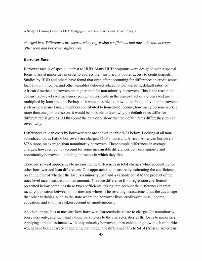
A Study of Closing Costs for FHA Mortgages: Part B — Lender and Broker Charges
charged less. Differences are measured as regression coefficients and thus take into account other loan and borrower differences.
Borrower Race
Borrower race is of special interest to HUD. Many HUD programs were designed with a special focus to assist minorities in order to address their historically poorer access to credit markets. Studies by HUD and others have found that even after accounting for differences in credit scores, loan amount, income, and other variables believed related to loan defaults, default rates for African American borrowers are higher than for non minority borrowers. This is the reason the census tract–level race measures (percent of residents in the census tract of a given race) are multiplied by loan amount. Perhaps if it were possible to know more about individual borrowers, such as how many family members contributed to household income, how many persons worked more than one job, and so on, it would be possible to learn why the default rates differ for different racial groups. At this point the data only show that the default rates differ; they do not reveal why.
Differences in loan costs by borrower race are shown in table 5-3a below. Looking at all non-subsidized loans, Latino borrowers are charged $1,043 more and African American borrowers $756 more, on average, than nonminority borrowers. These simple differences in average charges, however, do not account for some measurable differences between minority and nonminority borrowers, including the states in which they live.
There are several approaches to measuring the differences in total charges while accounting for other borrower and loan differences. One approach is to measure by estimating the coefficients on an indictor of whether the loan is a minority loan and a variable equal to the product of the tract-level race measure and loan amount. The race difference from regression coefficients presented below combines these two coefficients, taking into account the differences in tract racial composition between minorities and whites. The resulting measurement has the advantage that other variables, such as the state where the borrower lives, creditworthiness, income, education, and so on, are taken account of simultaneously.
Another approach is to measure how borrower characteristics relate to charges for nonminority borrowers only, and then apply those parameters to the characteristics of the loans to minorities. Applying a model estimated with only minority borrowers, then calculating how much minorities would have been charged if applying that model, the difference falls to $414 (African American)
45
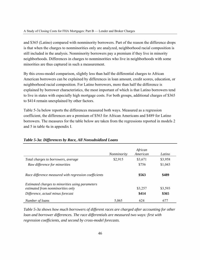
A Study of Closing Costs for FHA Mortgages: Part B — Lender and Broker Charges
and $365 (Latino) compared with nonminority borrowers. Part of the reason the difference drops is that when the charges to nonminorities only are analyzed, neighborhood racial composition is still included in the analysis. Nonminority borrowers pay a premium if they live in minority neighborhoods. Differences in charges to nonminorities who live in neighborhoods with some minorities are thus captured in such a measurement.
By this cross-model comparison, slightly less than half the differential charges to African American borrowers can be explained by differences in loan amount, credit scores, education, or neighborhood racial composition. For Latino borrowers, more than half the difference is explained by borrower characteristics, the most important of which is that Latino borrowers tend to live in states with especially high mortgage costs. For both groups, additional charges of $365 to $414 remain unexplained by other factors.
Table 5-3a below reports the differences measured both ways. Measured as a regression coefficient, the differences are a premium of $563 for African Americans and $489 for Latino borrowers. The measures for the table below are taken from the regressions reported in models 2 and 5 in table 4a in appendix I.
Table 5-3a: Differences by Race, All Nonsubsidized Loans
African Nonminority American Latino
Total charges to borrowers, average $2,915 $3,671 $3,958 Raw difference for minorities $756 $1,043
Race difference measured with regression coefficients $563 $489
Estimated charges to minorities using parameters estimated from nonminorities only $3,257 $3,593 Difference, actual minus forecast $414 $365
Number of loans 5,065 624 677
Table 5-3a shows how much borrowers of different races are charged after accounting for other loan and borrower differences. The race differentials are measured two ways: first with regression coefficients, and second by cross-model forecasts.
46
A Study of Closing Costs for FHA Mortgages: Part B — Lender and Broker Charges
Using only the loans with rates at seven percent and above, the absolute differences in how much borrowers of different race are charged is similar. The measures of differential treatment that take account of borrower differences are only slightly smaller than when all nonsubsidized loans, not just those at coupon rates above seven percent, are used.
Table 5-3b: Summary of Differences by Race, Nonsubsidized Loans with Rates above Seven Percent
Non-minority
African-American Latino
Total charges to borrowers, average $3,348 $4,048 $4,388 Raw difference for minorities $700 $1,040
Race difference measured with regression coefficients $532 $450
Estimated charges to nonsubsidized minorities using parameters estimated from nonminorities only $3,735 $4,098 Difference, actual minus forecast $313 $290
Number of loans 3,582 476 545
Table 5-3b shows the differences in how much borrowers of different races are charged after accounting for other loan and borrower differences, looking only at loans with coupons of seven percent or more. The race differentials are measured two ways: first with regression coefficients, and second by cross-model forecasts.
The interpretation of the race differentials cannot be entirely clear from the data available in this study. Differences could be related to different expected costs associated with different probabilities of default across by race. The discussion in the later chapter on defaults will reveal that borrowers who live in neighborhoods with a high fraction of African Americans have higher default likelihoods than do other borrowers, other things equal, while Latino borrowers have lower default likelihoods than other borrowers. Even for the brokered loans, it is not possible to know which loan origination charges were paid to the mortgage broker, who bears no costs in the case of a loan default, versus which were paid to the ultimate lender or servicer, who does bear the cost. While the YSPs are always paid to the mortgage broker, other cash fees (such as origination fee, underwriting fee, document preparation fee) could go to either broker or to the wholesale lender. Only records from the brokers or lenders can confirm who was paid what. As a
47
A Study of Closing Costs for FHA Mortgages: Part B — Lender and Broker Charges
result, it is not possible here to determine dispositively whether the higher fees charged to minority borrowers are the result of higher wholesale lender charges or higher broker charges.
In the studies of Cohen (2005) and Woodward (2003), data were available to isolate fees to brokers. Both of these studies found higher broker fees to African American borrowers. These studies point in the direction of at least part of the difference here also coming from price discrimination against minorities as less-price-elastic borrowers.
The differential fees for African American borrowers using all nonsubsidized loans, here $400 using all loans, is close to what was found in Woodward (2003), $500, and also by Cohen (2005), $500, in his auto loan study, even though the mortgage loan amounts in Woodward (2003) averaged $135,000 while the auto loans in Cohen (2005) averaged $23,000. Perhaps this coefficient measures the amount minority borrowers are willing to pay, in comparison with other borrowers, to not be subjected to the loan approval process one more time. Presumably all borrowers value their time and would prefer to spend it in some way other than making loan applications, and all prefer to not be rejected, but the borrowers who historically have been treated poorly by the market may have a greater distaste for continuing the loan search process and the disappointment and insult it might deliver.
Education
The ideal measure of education for learning how borrower education relates to the amounts borrowers pay would be the borrower’s own level of education. It might even be useful to know whether the borrower’s education had a quantitative emphasis. Lacking such detailed information on borrowers, instead this study uses as a measure of educational attainment the fraction of adults with a college education in the borrower’s census tract. If this measure is thought of as a proxy for the borrower’s education, it clearly measures that with some error.
The original motive for including education in the analysis of mortgage terms was to see if educational differences accounted for some of the race and ethnicity differences. They do not. For African American borrowers, including education increases the racial difference a small amount; for Latino borrowers, it decreases it a small amount. The more surprising finding is just how important is education itself: the measurements that do not account for state differences indicate that borrowers who live in a neighborhood where no adults have a college education pay an additional $1,700 for their loans, other things equal, compared to those who live in a neighborhood where all adults have a college education. This translates into a finding that a 10
48
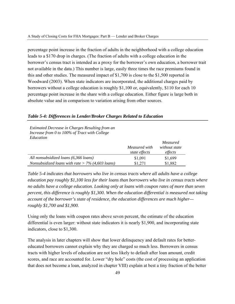
A Study of Closing Costs for FHA Mortgages: Part B — Lender and Broker Charges
percentage point increase in the fraction of adults in the neighborhood with a college education leads to a $170 drop in charges. (The fraction of adults with a college education in the borrower’s census tract is intended as a proxy for the borrower’s own education, a borrower trait not available in the data.) This number is large, easily three times the race premiums found in this and other studies. The measured impact of $1,700 is close to the $1,500 reported in Woodward (2003). When state indicators are incorporated, the additional charges paid by borrowers without a college education is roughly $1,100 or, equivalently, $110 for each 10 percentage point increase in the share with a college education. Either figure is large both in absolute value and in comparison to variation arising from other sources.
Table 5-4: Differences in Lender/Broker Charges Related to Education
Estimated Decrease in Charges Resulting from an Increase from 0 to 100% of Tract with College Education
Measured Measured with without state
state effects effects All nonsubsidized loans (6,366 loans) $1,091 $1,699 Nonsubsidized loans with rate > 7% (4,603 loans) $1,271 $1,882
Table 5-4 indicates that borrowers who live in census tracts where all adults have a college education pay roughly $1,100 less for their loans than borrowers who live in census tracts where no adults have a college education. Looking only at loans with coupon rates of more than seven percent, this difference is roughly $1,300. When the education differential is measured not taking account of the borrower’s state of residence, the education differences are much higher— roughly $1,700 and $1,900.
Using only the loans with coupon rates above seven percent, the estimate of the education differential is even larger: without state indicators it is nearly $1,900, and incorporating state indicators, close to $1,300.
The analysis in later chapters will show that lower delinquency and default rates for better-educated borrowers cannot explain why they are charged so much less. Borrowers in census tracts with higher levels of education are not less likely to default after loan amount, credit scores, and race are accounted for. Lower “dry hole” costs (the cost of processing an application that does not become a loan, analyzed in chapter VIII) explain at best a tiny fraction of the better
49
A Study of Closing Costs for FHA Mortgages: Part B — Lender and Broker Charges
terms enjoyed by better-educated borrowers. The measures supporting the figures in table 5-4 appear in the regression reported in models 1 and 2 in table 4a (for all loans) and table 4b (for loans with coupons over 7) in appendix I.
State Differences
In addition to the loan and borrower characteristics that explain substantial variation in lender/broker charges, the measurement includes categorical variables to measure differences by state. The state differences are large. The coefficients on the state categorical variables indicate that other things equal (especially loan amount, which captures differences across states in property values), borrowers in Nevada (the state with the highest lender/broker charges) pay more than $2,700 more to their brokers or lenders than borrowers in Alaska (the state with the lowest charges). The source of these substantial differences deserves investigation. The differences are too large to be merely random variation in the sample differences by state.
Differences in mortgage law by state could influence the costs lenders bear in the case of a loan default. One is that in some states, home mortgages are nonrecourse loans. This means that if the borrower defaults on the loan and moves out of the house, thus relinquishing the house to the lender, the lender cannot pursue the borrower for any other money. The lender has “no recourse” to the borrower except the house if the borrower fails to repay the loan. In other states, a borrower must declare personal bankruptcy to discharge mortgage debt.
Nonrecourse regimes lower the cost to borrowers of defaulting on a mortgage. Lender pricing must cover the expected cost of defaults. As a result, competitive forces should lead lenders to charge borrowers more in states where lenders have no recourse beyond the house. Eight states have nonrecourse mortgage law: Alaska, Arizona, California, Oregon, Minnesota, Montana, North Dakota, and Washington. All but two are western states, where lender/broker charges are high. Adding a categorical variable to the basic equation for measuring how loan and borrower characteristics relate to how much borrowers are charged (multiplied by loan amount, because a larger loan defaulted imposes higher costs on the lender), indicates clearly that the nonrecourse legal regime does raise costs to borrowers by $550 per $100,000 of loan amount.
The relationship between lender/broker charges and other loan and borrower characteristics are essentially unchanged by adding the nonrecourse variable. Only the state cost differentials change. The table below indicates the premium charged in each state compared with the lowest cost state, Alaska, when the nonrecourse variable is included.
50

A Study of Closing Costs for FHA Mortgages: Part B — Lender and Broker Charges
Table 5-5a: State Differences in Lender/Broker Charges, All Nonsubsidized Loans
Cost Cost Cost State premium State premium State premium Nevada Michigan Utah Florida Ohio New York Hawaii Maine Wisconsin District of Columbia Iowa Idaho West Virginia New Mexico Texas California
$2,739 $2,621 $2,596 $2,490 $2,403 $2,378 $2,351 $2,267 $2,229 $2,204 $2,181 $2,162 $2,106 $2,099 $2,099 $2,094 $2,094
Massachusetts Alabama Vermont Connecticut Washington Rhode Island Indiana Georgia Illinois North Carolina Pennsylvania Maryland Oklahoma Missouri South Dakota New Hampshire
$2,094 $2,014 $2,009 $1,998 $1,982 $1,981 $1,980 $1,973 $1,966 $1,954 $1,921 $1,878 $1,829 $1,813 $1,796 $1,769 $1,701
Kansas Virginia Colorado Delaware Arizona South Carolina Kentucky Arkansas Oregon Louisiana Nebraska Montana Minnesota Tennessee North Dakota Wyoming Alaska
$1,699 $1,697 $1,681 $1,656 $1,621 $1,610 $1,600 $1,566 $1,561 $1,534 $1,482 $1,464 $1,427 $1,289 $1,060 $1,049
$0New Jersey Mississippi
Table5-5a presents the differences in how much borrowers are charged, on average, across states, after accounting for other loan and borrower characteristics. The analysis uses all 6,366 nonsubsidized loans.
Table 5-5a above shows differences in lender/broker costs after taking into account other differences in loans and borrowers, such as loan amount. Borrowers in Nevada, Michigan, and Utah, pay a premium of more than $2,500 compared with Alaska. The regression for these measurements appears in model 3 in table 4a in appendix I.
It is also likely that state homestead exemptions from personal bankruptcy influence the likelihood of mortgage defaults and thus how much borrowers are charged. A large homestead exemption allows a borrower to declare personal bankruptcy and default on other personal debts without also defaulting on her mortgage, leaving her with more resources to make payments on her mortgage. A preliminary analysis, not included here, reveals that charges to borrowers are $500 lower in states where the homestead exemption is more than $40,000. Including a variable
51
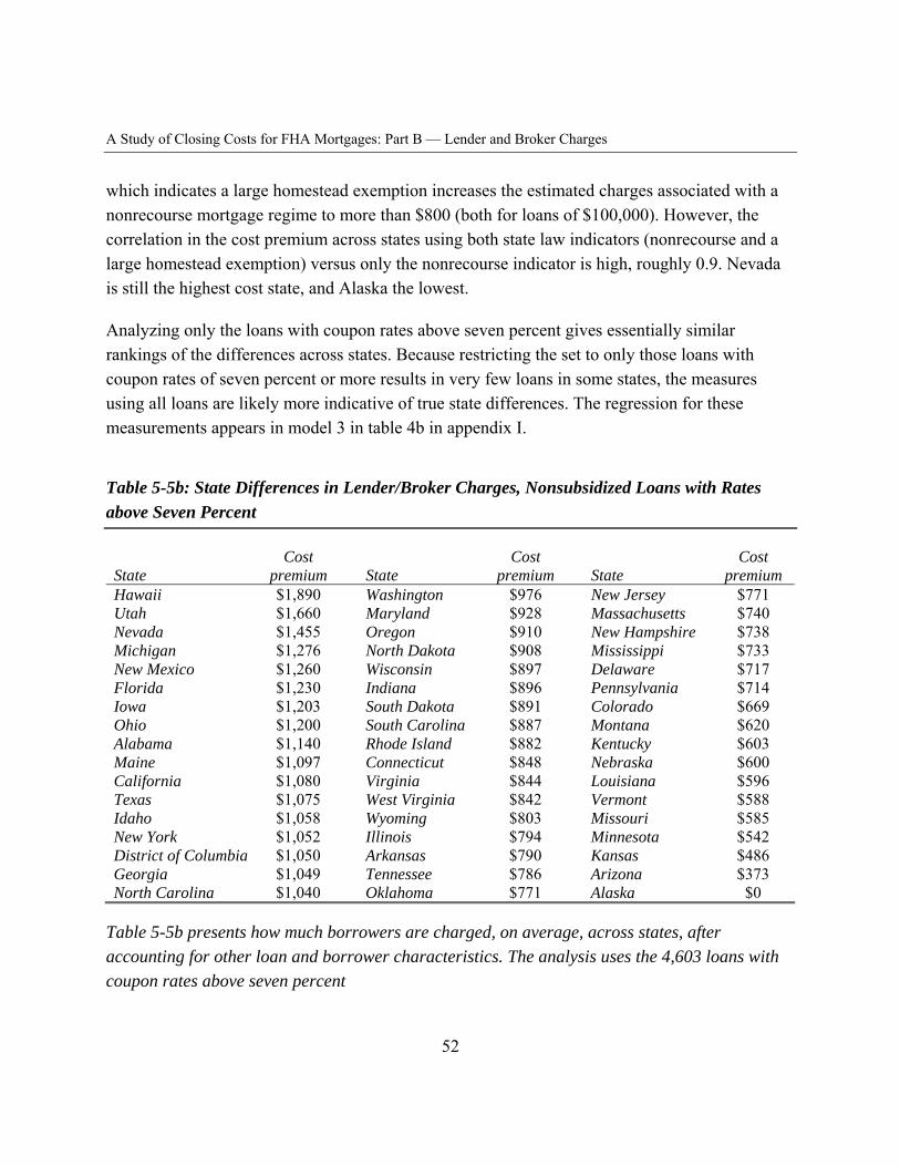
A Study of Closing Costs for FHA Mortgages: Part B — Lender and Broker Charges
which indicates a large homestead exemption increases the estimated charges associated with a nonrecourse mortgage regime to more than $800 (both for loans of $100,000). However, the correlation in the cost premium across states using both state law indicators (nonrecourse and a large homestead exemption) versus only the nonrecourse indicator is high, roughly 0.9. Nevada is still the highest cost state, and Alaska the lowest.
Analyzing only the loans with coupon rates above seven percent gives essentially similar rankings of the differences across states. Because restricting the set to only those loans with coupon rates of seven percent or more results in very few loans in some states, the measures using all loans are likely more indicative of true state differences. The regression for these measurements appears in model 3 in table 4b in appendix I.
Table 5-5b: State Differences in Lender/Broker Charges, Nonsubsidized Loans with Rates above Seven Percent
Cost Cost Cost State premium State premium State premium Hawaii $1,890 Washington $976 New Jersey $771 Utah $1,660 Maryland $928 Massachusetts $740 Nevada $1,455 Oregon $910 New Hampshire $738 Michigan $1,276 North Dakota $908 Mississippi $733 New Mexico $1,260 Wisconsin $897 Delaware $717 Florida $1,230 Indiana $896 Pennsylvania $714 Iowa $1,203 South Dakota $891 Colorado $669 Ohio $1,200 South Carolina $887 Montana $620 Alabama $1,140 Rhode Island $882 Kentucky $603 Maine $1,097 Connecticut $848 Nebraska $600 California $1,080 Virginia $844 Louisiana $596 Texas $1,075 West Virginia $842 Vermont $588 Idaho $1,058 Wyoming $803 Missouri $585 New York $1,052 Illinois $794 Minnesota $542 District of Columbia $1,050 Arkansas $790 Kansas $486 Georgia $1,049 Tennessee $786 Arizona $373 North Carolina $1,040 Oklahoma $771 Alaska $0
Table 5-5b presents how much borrowers are charged, on average, across states, after accounting for other loan and borrower characteristics. The analysis uses the 4,603 loans with coupon rates above seven percent
52
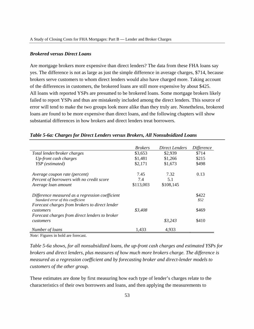
A Study of Closing Costs for FHA Mortgages: Part B — Lender and Broker Charges
Brokered versus Direct Loans
Are mortgage brokers more expensive than direct lenders? The data from these FHA loans say yes. The difference is not as large as just the simple difference in average charges, $714, because brokers serve customers to whom direct lenders would also have charged more. Taking account of the differences in customers, the brokered loans are still more expensive by about $425. All loans with reported YSPs are presumed to be brokered loans. Some mortgage brokers likely failed to report YSPs and thus are mistakenly included among the direct lenders. This source of error will tend to make the two groups look more alike than they truly are. Nonetheless, brokered loans are found to be more expensive than direct loans, and the following chapters will show substantial differences in how brokers and direct lenders treat borrowers.
Table 5-6a: Charges for Direct Lenders versus Brokers, All Nonsubsidized Loans
Brokers Direct Lenders Difference Total lender/broker charges $3,653 $2,939 $714
Up-front cash charges $1,481 $1,266 $215 YSP (estimated) $2,171 $1,673 $498
Average coupon rate (percent) 7.45 7.32 0.13 Percent of borrowers with no credit score 7.4 5.1 Average loan amount $113,003 $108,145
Difference measured as a regression coefficient $422 Standard error of this coefficient $52
Forecast charges from brokers to direct lender customers $3,408 $469 Forecast charges from direct lenders to broker customers $3,243 $410
Number of loans 1,433 4,933 Note: Figures in bold are forecast.
Table 5-6a shows, for all nonsubsidized loans, the up-front cash charges and estimated YSPs for brokers and direct lenders, plus measures of how much more brokers charge. The difference is measured as a regression coefficient and by forecasting broker and direct-lender models to customers of the other group.
These estimates are done by first measuring how each type of lender’s charges relate to the characteristics of their own borrowers and loans, and then applying the measurements to
53
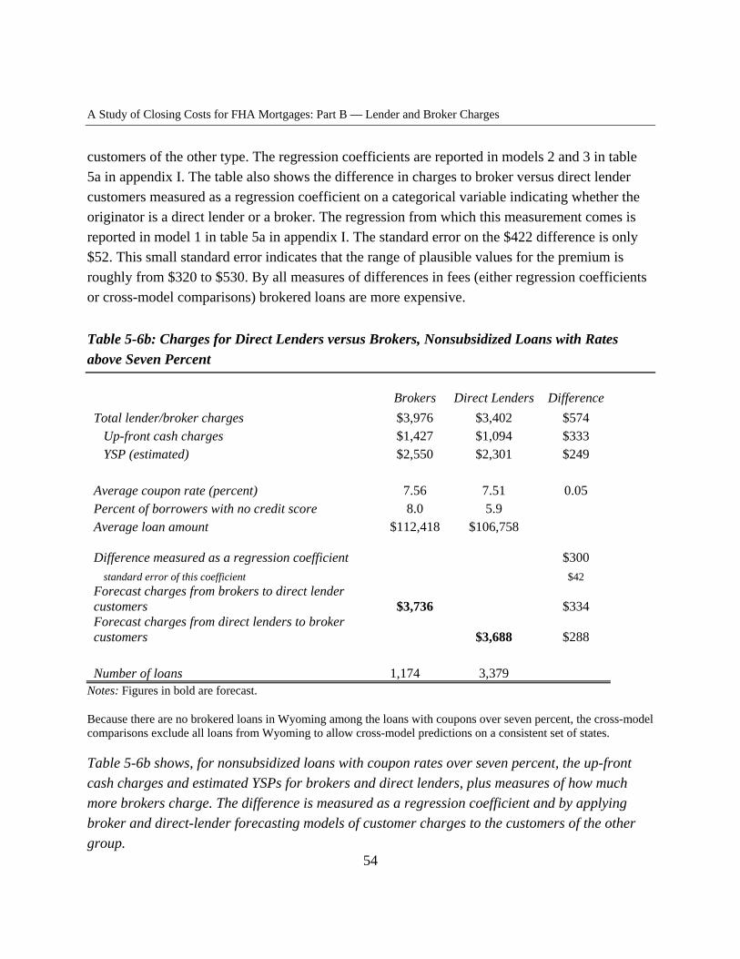
A Study of Closing Costs for FHA Mortgages: Part B — Lender and Broker Charges
customers of the other type. The regression coefficients are reported in models 2 and 3 in table 5a in appendix I. The table also shows the difference in charges to broker versus direct lender customers measured as a regression coefficient on a categorical variable indicating whether the originator is a direct lender or a broker. The regression from which this measurement comes is reported in model 1 in table 5a in appendix I. The standard error on the $422 difference is only $52. This small standard error indicates that the range of plausible values for the premium is roughly from $320 to $530. By all measures of differences in fees (either regression coefficients or cross-model comparisons) brokered loans are more expensive.
Table 5-6b: Charges for Direct Lenders versus Brokers, Nonsubsidized Loans with Rates above Seven Percent
Total lender/broker charges Up-front cash charges YSP (estimated)
Average coupon rate (percent) Percent of borrowers with no credit score Average loan amount
Difference measured as a regression coefficient standard error of this coefficient
Forecast charges from brokers to direct lender customers Forecast charges from direct lenders to broker customers
Number of loans
Brokers Direct Lenders Difference $3,976 $3,402 $574 $1,427 $1,094 $333 $2,550 $2,301 $249
7.56 7.51 0.05 8.0 5.9
$112,418 $106,758
$300 $42
$3,736 $334
$3,688 $288
1,174 3,379 Notes: Figures in bold are forecast.
Because there are no brokered loans in Wyoming among the loans with coupons over seven percent, the cross-model comparisons exclude all loans from Wyoming to allow cross-model predictions on a consistent set of states.
Table 5-6b shows, for nonsubsidized loans with coupon rates over seven percent, the up-front cash charges and estimated YSPs for brokers and direct lenders, plus measures of how much more brokers charge. The difference is measured as a regression coefficient and by applying broker and direct-lender forecasting models of customer charges to the customers of the other group.
54

A Study of Closing Costs for FHA Mortgages: Part B — Lender and Broker Charges
Why are brokered loans more expensive? The data show that roughly $300 of the difference is related to customer differences but cannot speak to the remainder. Perhaps brokers provide services other lenders do not. Perhaps the borrowers who go first to brokers do not know that better terms are available elsewhere. Perhaps brokers are more skilled salespeople. It is not possible to distinguish among these explanations using the data here.
Using only loans with coupon rates above seven percent, the difference in the cost of brokered versus direct loans is a bit smaller, roughly $300, as seen above in table 5-6b.
The regressions from which these measures are taken are reported in models 1 to 3 in table 5b of appendix I.
Loan Counseling
Information about loan counseling was available for most of the loans studied here. Among 7,560 loans, 155 borrowers were counseled by their own lender, 196 were counseled by third parties, 6,534 were offered counseling but declined it, and for 675 loans counseling information was missing. Among nonsubsidized loans, 101 borrowers had third-party counseling, and 120 had lender counseling.
Looking at all nonsubsidized loans, charges are lower to borrowers who received third-party counseling by $306 (t = -2.01) and to those who received counseling from their own lenders by $113 (t = -0.76). While these savings are not trivial, the test statistics indicate they are not very systematic. Nonetheless, the savings, combined with the low frequency of third-party counseling (only 101 nonsubsidized loans), suggest that additional investigation is in order before dismissing the value of counseling. Few borrowers among the loans with coupons above seven percent received counseling, and no benefit from counseling can be detected among these loans. The measures for this analysis appear in the regressions reported in model 1 of tables 6a and 6b in appendix I.
Some other variables that were studied but dropped for additional analysis are the dollar amount of the borrower’s down payment, the loan-to-value ratio, borrower gender (male versus female), borrower age, and the dollar balance and number of other debts paid off as part of the loan closing. The only one of these variables with any relation to how much borrowers pay is borrower age. The estimated coefficient on age is about $50 per decade, suggesting that a borrower age 60 would be charged $150 more than a borrower age 30. This variable explained
55
A Study of Closing Costs for FHA Mortgages: Part B — Lender and Broker Charges
only a tiny amount of additional variation and exhibited no interaction with other variables, and was thus dropped for the rest of the analysis.
Other studies have found loan charges relate to down payment and to loan-to-value ratios (LTVs), mainly because loans with larger down payments are less likely to default. Nearly all FHA purchase loans have very small down payments and thus very high LTVs, so perhaps there is just not enough variation in LTV to detect the relationship between LTV and lender charges.
56
A Study of Closing Costs for FHA Mortgages: Part B — Lender and Broker Charges
Chapter VI: Sources of Complexity and Confusion: Yield-spread Premiums, Discount Points, and Seller Contributions
Yield-Spread Premiums
When mortgage brokers became a significant source of origination services, controversy soon arose over how they are compensated. In particular, yield-spread premiums paid by wholesale lenders to mortgage brokers have been cast in litigation as kickbacks prohibited by RESPA. The objection to YSP payments arises partly because they give the mortgage broker an explicit incentive to persuade the borrower to take a loan with a higher interest rate. In principle, the incentives of mortgage brokers are no different from those of direct lenders, or any other sellers in the economy—all sellers prefer to sell at a higher price. Mortgage brokers, however, might pose as the borrower’s agent, claiming to search out many lenders for better terms for their customers. It is true that mortgage brokers see rates from multiple lenders, but as a general matter, the broker is not the borrower’s agent. Thus, it is of interest how borrower loan costs vary by the sources of compensation of the lender/broker, and by the type of lender. The analysis in chapter V showed that brokered loans are more expensive than direct loans, other factors equal. This chapter explores some of the factors that contribute to higher fees on brokered loans.
There are 1,799 different lenders represented among the loans studied here. It is thus feasible, based on lender names, to categorize lenders as depositories (banks, thrifts, and credit unions), mortgage brokers (those with reported YSP), and large versus smaller mortgage banks (based on the number of loans in the data). Among the lenders, six institutions each originated more than 100 loans; together, these lenders originated 2,161 of the 6,366 nonsubsidized loans. The six lenders with more than 100 loans each are designated as “large.” Institutions are thus categorized as mortgage brokers (any loan on which YSP is reported), depositories (identified by names that are restricted to depositories), large mortgage banks (non-depository, non-mortgage broker, more than 100 loans in the data set), and smaller mortgage banks (all others). There are systematic differences across types of lenders at a more detailed level than simply direct versus brokered loans.
If mortgage lending works as a well-informed, competitive market in which borrowers are able to effectively compare interest rate to up-front cash payments, one would expect that the market’s treatment of cash versus yield-spread premiums would be like the treatment of $10 bills versus $20 bills in other markets, or payment by cash versus by check, or cash versus credit
57

A Study of Closing Costs for FHA Mortgages: Part B — Lender and Broker Charges
card—the total charges should be same regardless of the form in which payment is delivered. To assess whether this is the case, the actual or estimated YSP is added as an explanatory variable to the regression of total charges on loan and borrower characteristics. If the YSP and borrower cash are exchanged in this market one-for-one, the measured change in total charges for a $100 change in YSP (the coefficient on the YSP) should be zero. In other words, when the borrower accepts a higher interest rate, the associated YSP would offset or reduce direct cash payments by the same amount, leaving total charges unchanged.
The data reveal a market far from the transparent and competitive ideal. The YSP is not just another way of compensating lenders. The change in total charges for a $1 change in YSP is not zero; indeed, as suggested by the plot analysis in chapter III, it is closer to $1 than to zero. It is closest to one for mortgage brokers, but closer to one than to zero for all four groups of lenders. The YSP is unambiguously a costly source of cash for most FHA borrowers. On average across all nonsubsidized loans, borrowers see up-front cash savings of roughly $20 for each $100 paid in YSP. This implies that for each $100 of YSP paid implicitly by borrowers in a higher interest rate, the borrower’s total costs rise by a bit more than $80. The borrowers’ net loss of $80 is the lender or brokers’ gain.
Table 6-1 shows the cost of the YSP to borrowers through different types of lenders. Borrowers see cash payments reduced by only $7 per $100 of YSP with mortgage brokers, for a net loss of $93: each $100 of YSP raises the present value of the borrower’s additional mortgage payments by $100; for paying a YSP of $100 the borrower saves $7 in up-front cash, so on net, the borrower’s total cost rises by $93. The borrower spends $100 in present-value, higher future payments to save $7 in cash now.
58
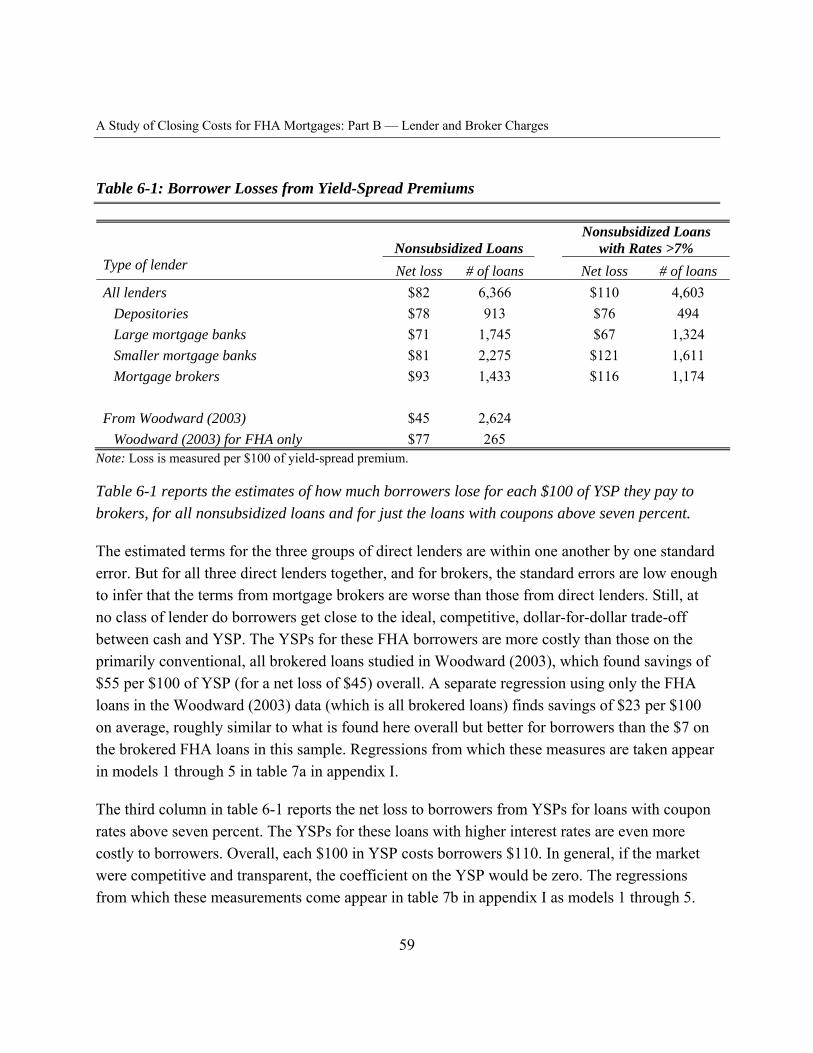
A Study of Closing Costs for FHA Mortgages: Part B — Lender and Broker Charges
Table 6-1: Borrower Losses from Yield-Spread Premiums
Nonsubsidized Loans Nonsubsidized Loans with Rates >7%
Type of lender Net loss # of loans Net loss # of loans All lenders
Depositories Large mortgage banks Smaller mortgage banks Mortgage brokers
From Woodward (2003)
$82 6,366 $78 913 $71 1,745 $81 2,275 $93 1,433
$110 4,603 $76 494 $67 1,324
$121 1,611 $116 1,174
$45 2,624 $77 265Woodward (2003) for FHA only
Note: Loss is measured per $100 of yield-spread premium.
Table 6-1 reports the estimates of how much borrowers lose for each $100 of YSP they pay to brokers, for all nonsubsidized loans and for just the loans with coupons above seven percent.
The estimated terms for the three groups of direct lenders are within one another by one standard error. But for all three direct lenders together, and for brokers, the standard errors are low enough to infer that the terms from mortgage brokers are worse than those from direct lenders. Still, at no class of lender do borrowers get close to the ideal, competitive, dollar-for-dollar trade-off between cash and YSP. The YSPs for these FHA borrowers are more costly than those on the primarily conventional, all brokered loans studied in Woodward (2003), which found savings of $55 per $100 of YSP (for a net loss of $45) overall. A separate regression using only the FHA loans in the Woodward (2003) data (which is all brokered loans) finds savings of $23 per $100 on average, roughly similar to what is found here overall but better for borrowers than the $7 on the brokered FHA loans in this sample. Regressions from which these measures are taken appear in models 1 through 5 in table 7a in appendix I.
The third column in table 6-1 reports the net loss to borrowers from YSPs for loans with coupon rates above seven percent. The YSPs for these loans with higher interest rates are even more costly to borrowers. Overall, each $100 in YSP costs borrowers $110. In general, if the market were competitive and transparent, the coefficient on the YSP would be zero. The regressions from which these measurements come appear in table 7b in appendix I as models 1 through 5.
59
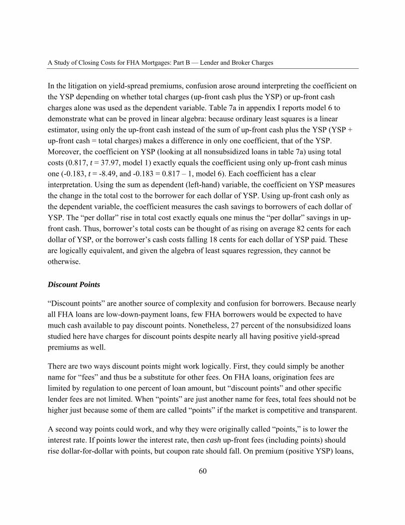
A Study of Closing Costs for FHA Mortgages: Part B — Lender and Broker Charges
In the litigation on yield-spread premiums, confusion arose around interpreting the coefficient on the YSP depending on whether total charges (up-front cash plus the YSP) or up-front cash charges alone was used as the dependent variable. Table 7a in appendix I reports model 6 to demonstrate what can be proved in linear algebra: because ordinary least squares is a linear estimator, using only the up-front cash instead of the sum of up-front cash plus the YSP (YSP + up-front cash = total charges) makes a difference in only one coefficient, that of the YSP. Moreover, the coefficient on YSP (looking at all nonsubsidized loans in table 7a) using total costs (0.817, t = 37.97, model 1) exactly equals the coefficient using only up-front cash minus one (-0.183, t = -8.49, and -0.183 = 0.817 – 1, model 6). Each coefficient has a clear interpretation. Using the sum as dependent (left-hand) variable, the coefficient on YSP measures the change in the total cost to the borrower for each dollar of YSP. Using up-front cash only as the dependent variable, the coefficient measures the cash savings to borrowers of each dollar of YSP. The “per dollar” rise in total cost exactly equals one minus the “per dollar” savings in upfront cash. Thus, borrower’s total costs can be thought of as rising on average 82 cents for each dollar of YSP, or the borrower’s cash costs falling 18 cents for each dollar of YSP paid. These are logically equivalent, and given the algebra of least squares regression, they cannot be otherwise.
Discount Points
“Discount points” are another source of complexity and confusion for borrowers. Because nearly all FHA loans are low-down-payment loans, few FHA borrowers would be expected to have much cash available to pay discount points. Nonetheless, 27 percent of the nonsubsidized loans studied here have charges for discount points despite nearly all having positive yield-spread premiums as well.
There are two ways discount points might work logically. First, they could simply be another name for “fees” and thus be a substitute for other fees. On FHA loans, origination fees are limited by regulation to one percent of loan amount, but “discount points” and other specific lender fees are not limited. When “points” are just another name for fees, total fees should not be higher just because some of them are called “points” if the market is competitive and transparent.
A second way points could work, and why they were originally called “points,” is to lower the interest rate. If points lower the interest rate, then cash up-front fees (including points) should rise dollar-for-dollar with points, but coupon rate should fall. On premium (positive YSP) loans,
60
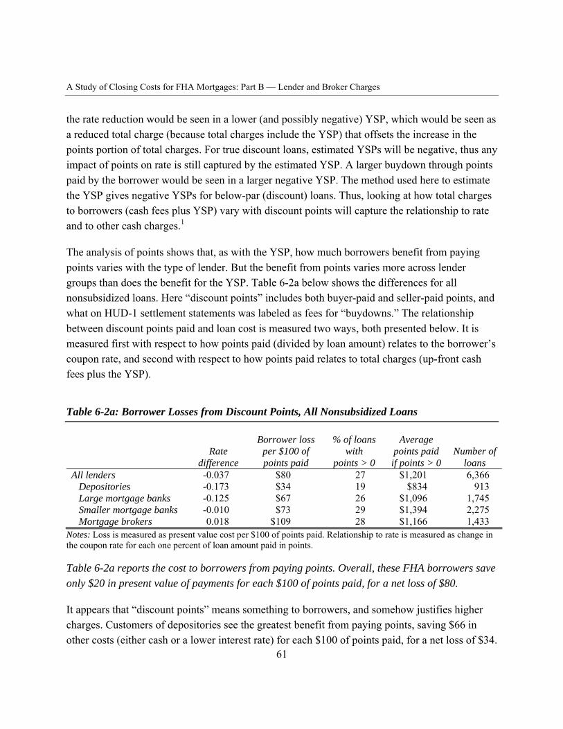
A Study of Closing Costs for FHA Mortgages: Part B — Lender and Broker Charges
the rate reduction would be seen in a lower (and possibly negative) YSP, which would be seen as a reduced total charge (because total charges include the YSP) that offsets the increase in the points portion of total charges. For true discount loans, estimated YSPs will be negative, thus any impact of points on rate is still captured by the estimated YSP. A larger buydown through points paid by the borrower would be seen in a larger negative YSP. The method used here to estimate the YSP gives negative YSPs for below-par (discount) loans. Thus, looking at how total charges to borrowers (cash fees plus YSP) vary with discount points will capture the relationship to rate and to other cash charges.1
The analysis of points shows that, as with the YSP, how much borrowers benefit from paying points varies with the type of lender. But the benefit from points varies more across lender groups than does the benefit for the YSP. Table 6-2a below shows the differences for all nonsubsidized loans. Here “discount points” includes both buyer-paid and seller-paid points, and what on HUD-1 settlement statements was labeled as fees for “buydowns.” The relationship between discount points paid and loan cost is measured two ways, both presented below. It is measured first with respect to how points paid (divided by loan amount) relates to the borrower’s coupon rate, and second with respect to how points paid relates to total charges (up-front cash fees plus the YSP).
Table 6-2a: Borrower Losses from Discount Points, All Nonsubsidized Loans
Borrower loss % of loans Average Rate per $100 of with points paid Number of
difference points paid points > 0 if points > 0 loans All lenders -0.037 $80 27 $1,201 6,366
Depositories -0.173 $34 19 $834 913 Large mortgage banks -0.125 $67 26 $1,096 1,745 Smaller mortgage banks -0.010 $73 29 $1,394 2,275 Mortgage brokers 0.018 $109 28 $1,166 1,433
Notes: Loss is measured as present value cost per $100 of points paid. Relationship to rate is measured as change in the coupon rate for each one percent of loan amount paid in points.
Table 6-2a reports the cost to borrowers from paying points. Overall, these FHA borrowers save only $20 in present value of payments for each $100 of points paid, for a net loss of $80.
It appears that “discount points” means something to borrowers, and somehow justifies higher charges. Customers of depositories see the greatest benefit from paying points, saving $66 in other costs (either cash or a lower interest rate) for each $100 of points paid, for a net loss of $34.
61
A Study of Closing Costs for FHA Mortgages: Part B — Lender and Broker Charges
Borrowers get the worst terms from paying points to mortgage brokers; they pay an extra $109 in total costs for each $100 paid in points. With mortgage brokers, both total charges and rates rise instead of falling with points paid—or, expressed another way, the coupon rate is higher instead of lower, or other cash fees are higher instead of lower, when broker customers pay points. At both large and smaller mortgage banks, borrowers see a decline in rate or other cash costs when they pay points but less than at depositories. Thus, in no case does the measured benefit of paying points exceed or equal the cost. The coefficients for large versus smaller mortgage banks are less than one standard error apart, indicating little statistically detectable difference. Regressions supporting these measurements appear in models 1 through 5 in tables 8a (on rates) and 9a (on total charges) in appendix I.
Table 6-2b below shows the same measurements using only loans with coupons greater than seven percent. For the higher-rate loans, overall points raise costs rather than lower them. Only at depositories and large mortgage banks do borrowers see any benefit from points; even for these, the benefits are small. Regressions supporting these measurements appear in models 1 through 5 in tables 8b and 9b in appendix I.
Table 6-2b: Borrower Losses from Discount Points to Borrowers, Nonsubsidized Loans with Rates above Seven Percent
Borrower loss % of loans Rate per $100 of with Average
difference points paid points > 0 points paid # of loans All lenders 0.070 $115 22 $1,185 4,603
Depositories -0.006 $96 10 $740 494 Large mortgage banks -0.008 $93 19 $938 1,324 Smaller mortgage banks 0.091 $111 25 $1,388 1,611 Mortgage brokers 0.067 $121 26 $1,198 1,174
Notes: Impact is measured as present value cost per $100 of points paid. Impact on rate is measured as change in the coupon rate for each one percent of loan amount paid in points.
Table 6-2b reports the costs to borrowers from paying points on loans with coupon rates above seven percent. Overall, these FHA borrowers pay an extra $15 in present value of payments beyond each $100 of points paid, for a net loss of $115.
As with the analysis of yield-spread premiums, the analysis of discount points paid by borrowers with coupon rates over 7 percent present an even less borrower-friendly lending environment.
62
A Study of Closing Costs for FHA Mortgages: Part B — Lender and Broker Charges
Again, this is not just because these are higher-rate loans. If “discount points” was just another name for origination fees, and loans with points had no origination fees, discount points would not cost borrowers anything, because total (up-front cash) origination fees would be unrelated to the names given these fees.
Seller Contribution
The FHA mortgage market is unique in that sellers frequently contribute to the buyer’s closing costs—on 75 percent of the loans studied here. In the conventional mortgage loan market, sellers typically pay for only the services of the real estate agent, and in some states, for the lender’s title insurance. How much buyers benefit from seller contributions can, as for YSPs and discount points, be measured and evaluated from the perspective of a fully informed competitive market, again from the perspective of whether they are treated as similarly as $10 versus $20 dollar bills, or checks versus cash versus credit cards, and so on. In such a market, the combined costs on the loan and the house together would not relate to where the money comes from—the buyer, the lender in the form of a YSP, or the seller. The buyer and seller would dicker over house price versus seller contribution to closing costs, but the total cost of the house and the loan should be unchanged. It should not matter whether the seller’s contribution is to closing costs or specifically to points. Either should reduce the buyer’s cash needs or, if more cash is paid up front, the buyer’s interest rate.
The trade-off of house prices to seller contributions to the loan terms is an abiding issue at FHA. FHA’s main concern regarding seller contributions is whether the borrower pays a higher price for the house in exchange for the seller contribution. The question arises in the context of a transaction of this sort: the seller wants $100,000 for the house. Suppose the buyer has only $2,500 cash for closing costs plus down payment. If the house price is adjusted upwards by, for example, $2,000, and the seller agrees to contribute $2,000 to closing costs, then the buyer now has a $2,500 down payment, closing costs are covered by the seller’s $2,000, the seller gets her desired $100,000 (the $102,000 “selling price” less the $2,000 contribution to closing costs), and FHA insures a larger loan. Here is the problem: the house is not really $2,000 more valuable as a result of arranging the transaction this way. If the house were resold the next week, it would not be expected to fetch $102,000, but the market value of $100,000. The true loan-to-value ratio is thus understated (appearing lower than it truly is) when seller contributions inflate the selling price of the house, making FHA’s default exposure greater. FHA thus has an interest in either prohibiting seller contributions in exchange for a higher house price or in adjusting its insurance
63
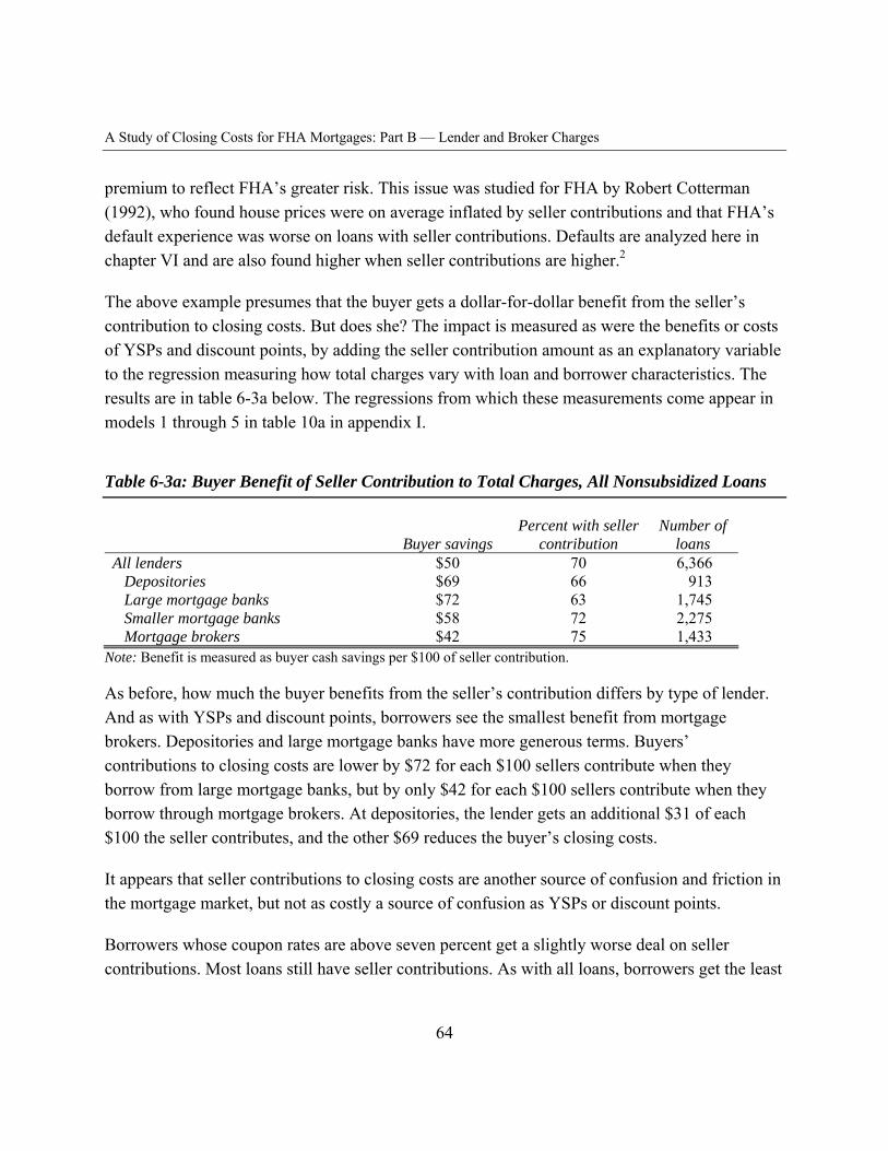
A Study of Closing Costs for FHA Mortgages: Part B — Lender and Broker Charges
premium to reflect FHA’s greater risk. This issue was studied for FHA by Robert Cotterman (1992), who found house prices were on average inflated by seller contributions and that FHA’s default experience was worse on loans with seller contributions. Defaults are analyzed here in chapter VI and are also found higher when seller contributions are higher.2
The above example presumes that the buyer gets a dollar-for-dollar benefit from the seller’s contribution to closing costs. But does she? The impact is measured as were the benefits or costs of YSPs and discount points, by adding the seller contribution amount as an explanatory variable to the regression measuring how total charges vary with loan and borrower characteristics. The results are in table 6-3a below. The regressions from which these measurements come appear in models 1 through 5 in table 10a in appendix I.
Table 6-3a: Buyer Benefit of Seller Contribution to Total Charges, All Nonsubsidized Loans
Percent with seller Number of Buyer savings contribution loans
All lenders $50 70 6,366 Depositories $69 66 913 Large mortgage banks $72 63 1,745 Smaller mortgage banks $58 72 2,275 Mortgage brokers $42 75 1,433
Note: Benefit is measured as buyer cash savings per $100 of seller contribution.
As before, how much the buyer benefits from the seller’s contribution differs by type of lender. And as with YSPs and discount points, borrowers see the smallest benefit from mortgage brokers. Depositories and large mortgage banks have more generous terms. Buyers’ contributions to closing costs are lower by $72 for each $100 sellers contribute when they borrow from large mortgage banks, but by only $42 for each $100 sellers contribute when they borrow through mortgage brokers. At depositories, the lender gets an additional $31 of each $100 the seller contributes, and the other $69 reduces the buyer’s closing costs.
It appears that seller contributions to closing costs are another source of confusion and friction in the mortgage market, but not as costly a source of confusion as YSPs or discount points.
Borrowers whose coupon rates are above seven percent get a slightly worse deal on seller contributions. Most loans still have seller contributions. As with all loans, borrowers get the least
64
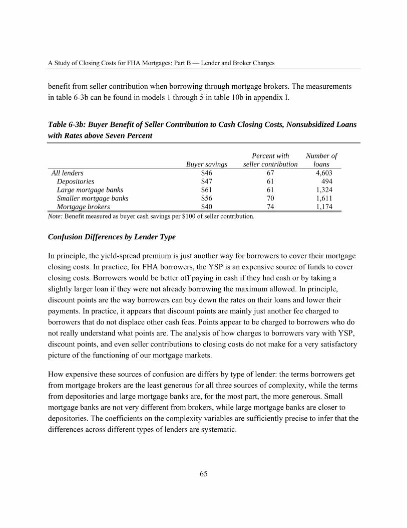
A Study of Closing Costs for FHA Mortgages: Part B — Lender and Broker Charges
benefit from seller contribution when borrowing through mortgage brokers. The measurements in table 6-3b can be found in models 1 through 5 in table 10b in appendix I.
Table 6-3b: Buyer Benefit of Seller Contribution to Cash Closing Costs, Nonsubsidized Loans with Rates above Seven Percent
Percent with Number of Buyer savings seller contribution loans
All lenders $46 67 4,603 Depositories $47 61 494 Large mortgage banks $61 61 1,324 Smaller mortgage banks $56 70 1,611 Mortgage brokers $40 74 1,174
Note: Benefit measured as buyer cash savings per $100 of seller contribution.
Confusion Differences by Lender Type
In principle, the yield-spread premium is just another way for borrowers to cover their mortgage closing costs. In practice, for FHA borrowers, the YSP is an expensive source of funds to cover closing costs. Borrowers would be better off paying in cash if they had cash or by taking a slightly larger loan if they were not already borrowing the maximum allowed. In principle, discount points are the way borrowers can buy down the rates on their loans and lower their payments. In practice, it appears that discount points are mainly just another fee charged to borrowers that do not displace other cash fees. Points appear to be charged to borrowers who do not really understand what points are. The analysis of how charges to borrowers vary with YSP, discount points, and even seller contributions to closing costs do not make for a very satisfactory picture of the functioning of our mortgage markets.
How expensive these sources of confusion are differs by type of lender: the terms borrowers get from mortgage brokers are the least generous for all three sources of complexity, while the terms from depositories and large mortgage banks are, for the most part, the more generous. Small mortgage banks are not very different from brokers, while large mortgage banks are closer to depositories. The coefficients on the complexity variables are sufficiently precise to infer that the differences across different types of lenders are systematic.
65
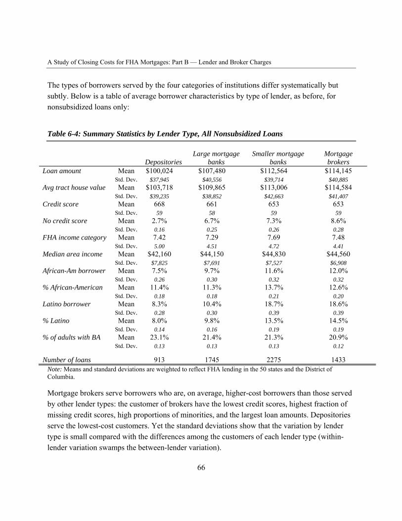
A Study of Closing Costs for FHA Mortgages: Part B — Lender and Broker Charges
The types of borrowers served by the four categories of institutions differ systematically but subtly. Below is a table of average borrower characteristics by type of lender, as before, for nonsubsidized loans only:
Table 6-4: Summary Statistics by Lender Type, All Nonsubsidized Loans
Large mortgage Smaller mortgage Mortgage Depositories banks banks brokers
Loan amount
Avg tract house value
Credit score
No credit score
FHA income category
Median area income
African-Am borrower
% African-American
Latino borrower
% Latino
% of adults with BA
Number of loans
Mean $100,024 $107,480 $112,564 $114,145 Std. Dev. $37,945 $40,556 $39,714 $40,885 Mean $103,718 $109,865 $113,006 $114,584
Std. Dev. $39,235 $38,852 $42,663 $41,407 Mean 668 661 653 653
Std. Dev. 59 58 59 59 Mean 2.7% 6.7% 7.3% 8.6%
Std. Dev. 0.16 0.25 0.26 0.28 Mean 7.42 7.29 7.69 7.48
Std. Dev. 5.00 4.51 4.72 4.41 Mean $42,160 $44,150 $44,830 $44,560
Std. Dev. $7,825 $7,691 $7,527 $6,908 Mean 7.5% 9.7% 11.6% 12.0%
Std. Dev. 0.26 0.30 0.32 0.32 Mean 11.4% 11.3% 13.7% 12.6%
Std. Dev. 0.18 0.18 0.21 0.20 Mean 8.3% 10.4% 18.7% 18.6%
Std. Dev. 0.28 0.30 0.39 0.39 Mean 8.0% 9.8% 13.5% 14.5%
Std. Dev. 0.14 0.16 0.19 0.19 Mean 23.1% 21.4% 21.3% 20.9%
Std. Dev. 0.13 0.13 0.13 0.12
913 1745 2275 1433 Note: Means and standard deviations are weighted to reflect FHA lending in the 50 states and the District of Columbia.
Mortgage brokers serve borrowers who are, on average, higher-cost borrowers than those served by other lender types: the customer of brokers have the lowest credit scores, highest fraction of missing credit scores, high proportions of minorities, and the largest loan amounts. Depositories serve the lowest-cost customers. Yet the standard deviations show that the variation by lender type is small compared with the differences among the customers of each lender type (withinlender variation swamps the between-lender variation).
66
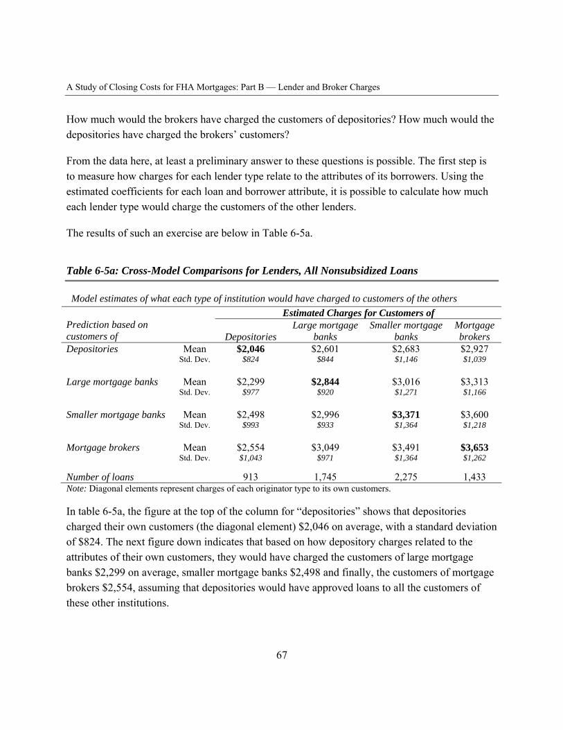
A Study of Closing Costs for FHA Mortgages: Part B — Lender and Broker Charges
How much would the brokers have charged the customers of depositories? How much would the depositories have charged the brokers’ customers?
From the data here, at least a preliminary answer to these questions is possible. The first step is to measure how charges for each lender type relate to the attributes of its borrowers. Using the estimated coefficients for each loan and borrower attribute, it is possible to calculate how much each lender type would charge the customers of the other lenders.
The results of such an exercise are below in Table 6-5a.
Table 6-5a: Cross-Model Comparisons for Lenders, All Nonsubsidized Loans
Model estimates of what each type of institution would have charged to customers of the others Estimated Charges for Customers of
Prediction based on customers of Depositories
Large mortgage banks
Smaller mortgage banks
Mortgage brokers
Depositories Mean Std. Dev.
$2,046 $824
$2,601 $844
$2,683 $1,146
$2,927 $1,039
Large mortgage banks Mean Std. Dev.
$2,299 $977
$2,844 $920
$3,016 $1,271
$3,313 $1,166
Smaller mortgage banks Mean Std. Dev.
$2,498 $993
$2,996 $933
$3,371 $1,364
$3,600 $1,218
Mortgage brokers Mean Std. Dev.
$2,554 $1,043
$3,049 $971
$3,491 $1,364
$3,653 $1,262
Number of loans 913 1,745 2,275 1,433 Note: Diagonal elements represent charges of each originator type to its own customers.
In table 6-5a, the figure at the top of the column for “depositories” shows that depositories charged their own customers (the diagonal element) $2,046 on average, with a standard deviation of $824. The next figure down indicates that based on how depository charges related to the attributes of their own customers, they would have charged the customers of large mortgage banks $2,299 on average, smaller mortgage banks $2,498 and finally, the customers of mortgage brokers $2,554, assuming that depositories would have approved loans to all the customers of these other institutions.
67
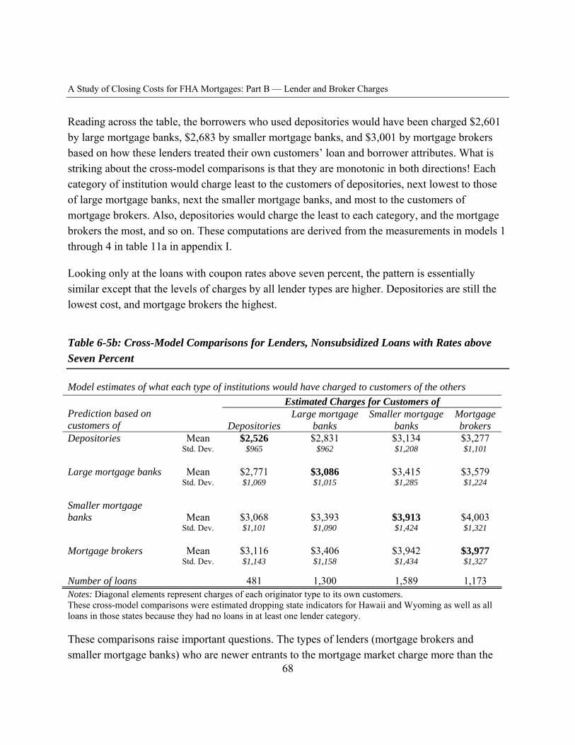
A Study of Closing Costs for FHA Mortgages: Part B — Lender and Broker Charges
Reading across the table, the borrowers who used depositories would have been charged $2,601 by large mortgage banks, $2,683 by smaller mortgage banks, and $3,001 by mortgage brokers based on how these lenders treated their own customers’ loan and borrower attributes. What is striking about the cross-model comparisons is that they are monotonic in both directions! Each category of institution would charge least to the customers of depositories, next lowest to those of large mortgage banks, next the smaller mortgage banks, and most to the customers of mortgage brokers. Also, depositories would charge the least to each category, and the mortgage brokers the most, and so on. These computations are derived from the measurements in models 1 through 4 in table 11a in appendix I.
Looking only at the loans with coupon rates above seven percent, the pattern is essentially similar except that the levels of charges by all lender types are higher. Depositories are still the lowest cost, and mortgage brokers the highest.
Table 6-5b: Cross-Model Comparisons for Lenders, Nonsubsidized Loans with Rates above Seven Percent
Model estimates of what each type of institutions would have charged to customers of the others Estimated Charges for Customers of
Prediction based on customers of Depositories
Large mortgage banks
Smaller mortgage banks
Mortgage brokers
Depositories Mean Std. Dev.
$2,526 $965
$2,831 $962
$3,134 $1,208
$3,277 $1,101
Large mortgage banks Mean Std. Dev.
$2,771 $1,069
$3,086 $1,015
$3,415 $1,285
$3,579 $1,224
Smaller mortgage banks Mean $3,068 $3,393 $3,913 $4,003
Std. Dev. $1,101 $1,090 $1,424 $1,321
Mortgage brokers Mean Std. Dev.
$3,116 $1,143
$3,406 $1,158
$3,942 $1,434
$3,977 $1,327
Number of loans 481 1,300 1,589 1,173 Notes: Diagonal elements represent charges of each originator type to its own customers. These cross-model comparisons were estimated dropping state indicators for Hawaii and Wyoming as well as all loans in those states because they had no loans in at least one lender category.
These comparisons raise important questions. The types of lenders (mortgage brokers and smaller mortgage banks) who are newer entrants to the mortgage market charge more than the
68
A Study of Closing Costs for FHA Mortgages: Part B — Lender and Broker Charges
ones that have been in existence longer. Depositories, which are the most heavily regulated of the four categories, are the lowest cost. Among the hypotheses that might explain these patterns are the following three:
1. The older types of institutions still have fairly rigid pricing and do not give their agents (loan officers) either the opportunity or the incentive to charge more to borrowers who might be confused about competitive terms. The newer types, especially mortgage brokers, are given fullest incentives to charge all the market will bear.
2. The older types of institutions serve their traditional customers, and the newer institutions serve customers previously not served by any lender.
3. Stango and Zinman (2006) suggest that less heavily regulated lenders engage in practices from which more regulated lenders refrain. They found that for consumer loans, banks appeared less inclined to exploit consumer confusion than did other types of lenders. Mortgage brokers are subject to little regulation. In principle, both large and smaller mortgage banks are subject to the same sort of regulation. But the larger institutions have more to lose from damage to their reputations or loss of their charters.
These hypotheses are not mutually exclusive.
The point of putting forth these hypotheses is not to determine which best fits the data, but simply to suggest possibilities for further study and reflection. The data available here cannot speak to these issues dispositively, but they can confirm systematic differences by lender type in how much borrowers are charged, and that differences relate to sources of borrower confusion.
In chapter VIII, defaults and dry-hole costs (the cost of processing applications that do not become loans) are examined for additional insight on why some borrowers are charged more than others, and why some types of lenders on average charge borrowers more than do others. Chapter VII on “no-cost” loans offers some insight as well.
69
A Study of Closing Costs for FHA Mortgages: Part B — Lender and Broker Charges
Chapter VII: A Source of Simplicity: The “No-cost” Loans
Among the 6,366 nonsubsidized loans are 495 in which all lender/broker fees were covered with a YSP. Borrowers do not arrive at such terms by happenstance but by seeking a “no-cost” loan. “No-cost” is of course a misnomer—it means that there are no up-front cash fees paid by the borrower or seller to the lender/broker. In principle, the rates on no-cost loans should be higher than the rates on loans with up-front fees, and they are. But all in, the terms on no-cost loans are substantially better than the terms on other loans.
“No-cost” loans are distinct in two important ways. First, they are cheaper than the other loans by about $1,200. Second, race and education premiums are nearly absent among the no-cost loans. Instead, charges are strongly related only to loan amount and credit scores.
These two findings suggest that the no-cost market is inherently more competitive than the wider mortgage market where borrowers pay some up-front cash. The findings also suggest that shopping complexity is a serious impediment to finding the competitive price. By requesting a no-cost loan, borrowers simplify their shopping because they can compare loans on rate alone, liberating themselves from struggling with up-front charges versus differences in interest rates. On a no-cost loan, a single number, the interest rate, is a sufficient statistic for comparing cost.
A borrower request for a no-cost loan may also inhibit the introduction of additional charges between application and closing. Other research suggests that such charges often do creep in. In Shroder’s (2007) study comparing Good Faith Estimates to the final charges on HUD-1s, he finds that additional fees are more likely when there are hints of difficulties (divorce, death in the family, very delinquent property taxes) in borrower lives. He also notes that courier and fax fees are very common entries on HUD-1s, but among more than 150 GFEs he studied, no such fees were included in estimated charges.
The simple difference in average charges for mortgages with no borrower cash payments to lender/brokers versus any-cash across all nonsubsidized loans is nearly $1,000. Measured as a regression coefficient, the difference is larger, $1,123, mainly because the loan amounts are larger for no-cost loans. The standard error on this coefficient is a remarkably small $70, indicating that the amount of the savings is highly systematic. Looking only at direct loans, the no-cost savings is a bit smaller, $1,064, and for brokered loans only, somewhat higher, $1,315. Even among no-cost loans, brokered loans are more expensive by $316, measured as a regression coefficient. Measures of the no-cost savings are essentially the same whether state-level effects
70
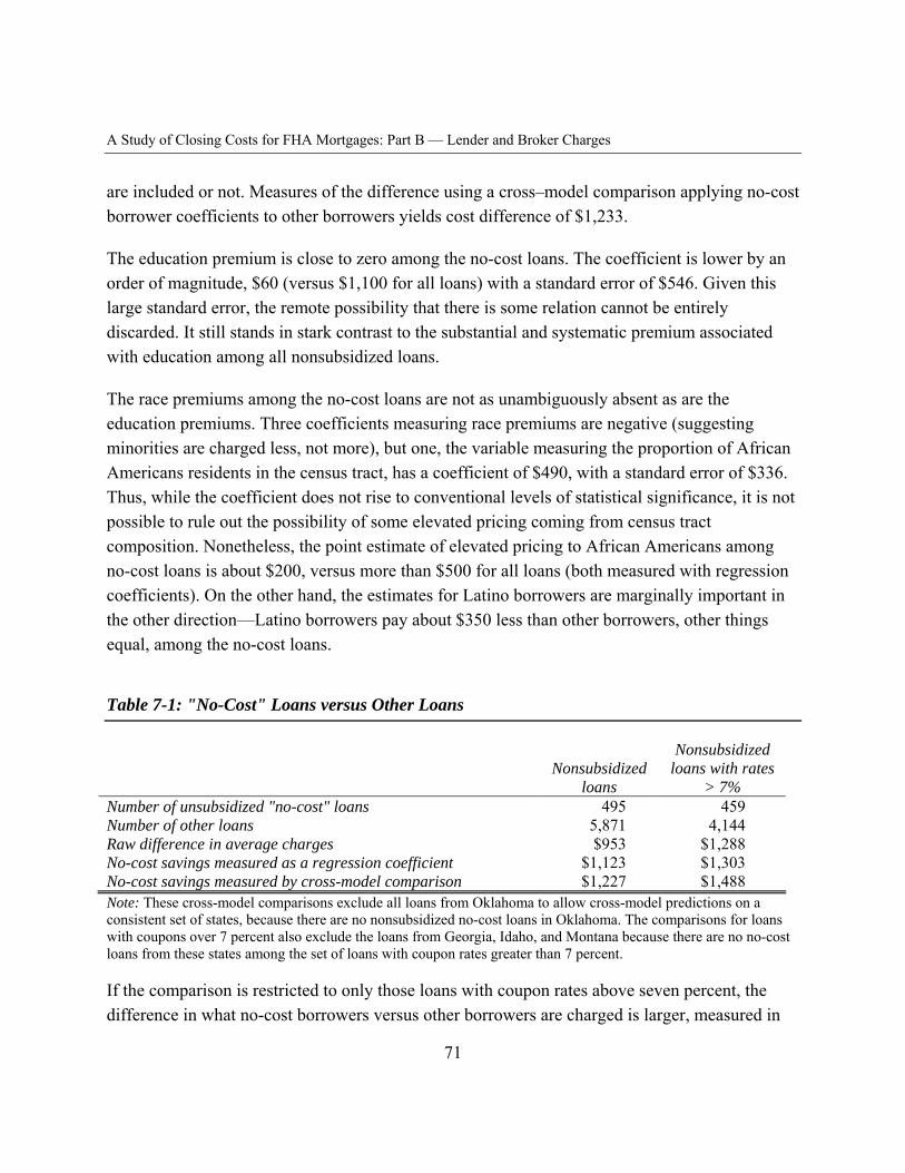
A Study of Closing Costs for FHA Mortgages: Part B — Lender and Broker Charges
are included or not. Measures of the difference using a cross–model comparison applying no-cost borrower coefficients to other borrowers yields cost difference of $1,233.
The education premium is close to zero among the no-cost loans. The coefficient is lower by an order of magnitude, $60 (versus $1,100 for all loans) with a standard error of $546. Given this large standard error, the remote possibility that there is some relation cannot be entirely discarded. It still stands in stark contrast to the substantial and systematic premium associated with education among all nonsubsidized loans.
The race premiums among the no-cost loans are not as unambiguously absent as are the education premiums. Three coefficients measuring race premiums are negative (suggesting minorities are charged less, not more), but one, the variable measuring the proportion of African Americans residents in the census tract, has a coefficient of $490, with a standard error of $336. Thus, while the coefficient does not rise to conventional levels of statistical significance, it is not possible to rule out the possibility of some elevated pricing coming from census tract composition. Nonetheless, the point estimate of elevated pricing to African Americans among no-cost loans is about $200, versus more than $500 for all loans (both measured with regression coefficients). On the other hand, the estimates for Latino borrowers are marginally important in the other direction—Latino borrowers pay about $350 less than other borrowers, other things equal, among the no-cost loans.
Table 7-1: "No-Cost" Loans versus Other Loans
Nonsubsidized Nonsubsidized loans with rates
loans > 7% Number of unsubsidized "no-cost" loans 495 459 Number of other loans 5,871 4,144 Raw difference in average charges $953 $1,288 No-cost savings measured as a regression coefficient $1,123 $1,303 No-cost savings measured by cross-model comparison $1,227 $1,488 Note: These cross-model comparisons exclude all loans from Oklahoma to allow cross-model predictions on a consistent set of states, because there are no nonsubsidized no-cost loans in Oklahoma. The comparisons for loans with coupons over 7 percent also exclude the loans from Georgia, Idaho, and Montana because there are no no-cost loans from these states among the set of loans with coupon rates greater than 7 percent.
If the comparison is restricted to only those loans with coupon rates above seven percent, the difference in what no-cost borrowers versus other borrowers are charged is larger, measured in
71
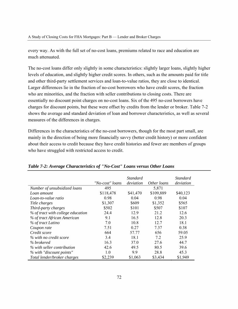
A Study of Closing Costs for FHA Mortgages: Part B — Lender and Broker Charges
every way. As with the full set of no-cost loans, premiums related to race and education are much attenuated.
The no-cost loans differ only slightly in some characteristics: slightly larger loans, slightly higher levels of education, and slightly higher credit scores. In others, such as the amounts paid for title and other third-party settlement services and loan-to-value ratios, they are close to identical. Larger differences lie in the fraction of no-cost borrowers who have credit scores, the fraction who are minorities, and the fraction with seller contributions to closing costs. There are essentially no discount point charges on no-cost loans. Six of the 495 no-cost borrowers have charges for discount points, but these were offset by credits from the lender or broker. Table 7-2 shows the average and standard deviation of loan and borrower characteristics, as well as several measures of the differences in charges.
Differences in the characteristics of the no-cost borrowers, though for the most part small, are mainly in the direction of being more financially savvy (better credit history) or more confident about their access to credit because they have credit histories and fewer are members of groups who have struggled with restricted access to credit.
Table 7-2: Average Characteristics of "No-Cost" Loans versus Other Loans
"No-cost" loans Standard deviation Other loans
Standard deviation
Number of unsubsidized loans 495 5,871 Loan amount $118,478 $41,470 $109,889 $40,123 Loan-to-value ratio 0.98 0.04 0.98 0.04 Title charges $1,307 $609 $1,352 $565 Third-party charges $502 $101 $507 $107 % of tract with college education 24.4 12.9 21.2 12.6 % of tract African American 9.1 16.5 12.8 20.3 % of tract Latino 7.0 10.8 12.7 18.1 Coupon rate 7.51 0.27 7.37 0.38 Credit score 664 57.77 656 59.05 % with no credit score 3.4 18.1 7.2 25.9 % brokered 16.3 37.0 27.6 44.7 % with seller contribution 42.6 49.5 80.5 39.6 % with "discount points" 1.0 9.9 28.8 45.3 Total lender/broker charges $2,239 $1,063 $3,434 $1,949
72
A Study of Closing Costs for FHA Mortgages: Part B — Lender and Broker Charges
Of course, the no-cost loans have higher interest rates than the other loans. The interest differential is accounted for in the computation of total charges by including the estimated YSP as part of lender/broker charges. Taking account of the higher interest rates on no-cost loans, the total cost for borrowers is still lower by about $1,200. Considering that the average borrower’s down payment is $2,500, this amount is substantial. Regression measurements appear in models 1 through 6 in table 12a in appendix I. For loans with coupon rates above seven percent, measurements are shown in models 1 through 6 in table 12b in appendix 1.
These measurements confirm those in Woodward (2003), which found similarly large savings for no-cost borrowers. The savings, plus—at least as important—the attenuation of race and education premiums among no-cost loans, are striking and important.
73
A Study of Closing Costs for FHA Mortgages: Part B — Lender and Broker Charges
Chapter VIII: Costs of Doing Business: Defaults and Dry Holes
In principle, competition should drive lender pricing to reflect the costs of doing business. Among the costs of doing business for mortgage lenders are dry holes—applications that are processed but fail to become loans—and defaults—loans on which the lender is not fully repaid. (The term “dry hole” comes from oil drilling—to fully cover cost, the driller must cover not only the cost of drilling and pumping from the successful wells but also the cost of drilling dry holes.) This chapter looks at how loan and borrower characteristics relate to expected default and dry-hole rates.
Defaults and Delinquencies
Defaults (loan foreclosures) and delinquencies are costly events for lenders, even on FHA-insured mortgage loans. Delinquencies generate costs because of the need to contact borrowers, and defaults result in some losses to the lender that FHA insurance does not cover. For what factors might lenders be adjusting pricing to reflect different likelihoods of delinquency and default? The mortgages studied here are old enough that the delinquencies and defaults to date can be related to loan and borrower characteristics.
Defaults are related to several factors, including one so far not much discussed: the number of consumer debt payoffs at closing. This information was collected from HUD-1 settlement statements. The number of items paid off (credit cards, consumer debts, individual store accounts, and so on) but not the total balance of these items is also related to delinquencies. This measure of credit quality was not used in the analysis of total charges because it was found to be unrelated to total charges for any loan or institution types despite its role as a predictor of defaults. One might think that a consumer who consolidates debts into a lower-rate loan might be a better credit risk. Instead, it appears that borrowers who are vulnerable to accumulating multiple debts but consolidate may be inclined to find themselves in the same situation again. The data cannot tell us why or how the borrowers with more numerous payoffs get into financial difficulties, but the data indicate that they do.
Delinquencies and foreclosures are lower for borrowers with larger loans and higher credit scores, and both are higher for borrowers with more debt payoffs at closing. Foreclosures are higher for borrowers lacking a credit score even after accounting for the predicted credit scores used here. Delinquencies and foreclosures are higher for borrowers who live in census tracts with
74

A Study of Closing Costs for FHA Mortgages: Part B — Lender and Broker Charges
a higher fraction of African American residents, but, importantly, not for individual African American borrowers. In other words, defaults for African American borrowers appear related to neighborhood racial composition, not individual borrower race. For Latino borrowers, foreclosures are lower, other things equal, than for other borrowers; for Latinos the relationship between defaults and race is detected at the individual borrower level, not at the census tract level. Delinquencies and foreclosures are also unrelated to the level of education for adults in the census tract (measured as a regression coefficient, so credit scores, neighborhood income levels, and loan amounts are accounted for simultaneously). Thus, differences in defaults and delinquencies cannot help us understand why borrowers from better-educated neighborhoods are charged so much less than other borrowers.
In addition, foreclosure rates are lower for borrowers who have higher seller-paid points on their loans but higher for larger seller contributions to closing costs. The second finding—higher default rates when sellers contribute more to closing costs—is also consistent with the findings of Cotterman (1992) and confirms FHA’s concern that seller contributions result in higher risk for FHA.
The relation of loan and borrower characteristics to defaults and delinquencies for loans with coupon rates over seven percent is similar to that for all nonsubsidized loans. All coefficients for the higher-interest loans have the same sign and are within one standard error of the corresponding coefficient for the full set.
The pattern of defaults in these FHA loans is familiar. Other studies of credit markets have also found defaults related to loan size, credit scores, and borrower race. The new findings here are
1. lower default rates for Latino borrowers are related to individual borrower race, not to neighborhood racial composition;
2. defaults rise with the number of loan payoffs at closing; and 3. there is no relationship between neighborhood education levels (measured as the fraction of
adults in the tract having completed college) and either delinquencies or defaults.
Regressions relating delinquencies and foreclosure rates to loan and borrower characteristics appear in models 1 and 2 in tables 13a and 13b in appendix I. An important implication of these results is that default patterns are in the same direction as some of, but not all, the differences in pricing by race. Still, the default patterns do not begin to explain the substantially better terms for borrowers in neighborhoods with higher education levels.
75
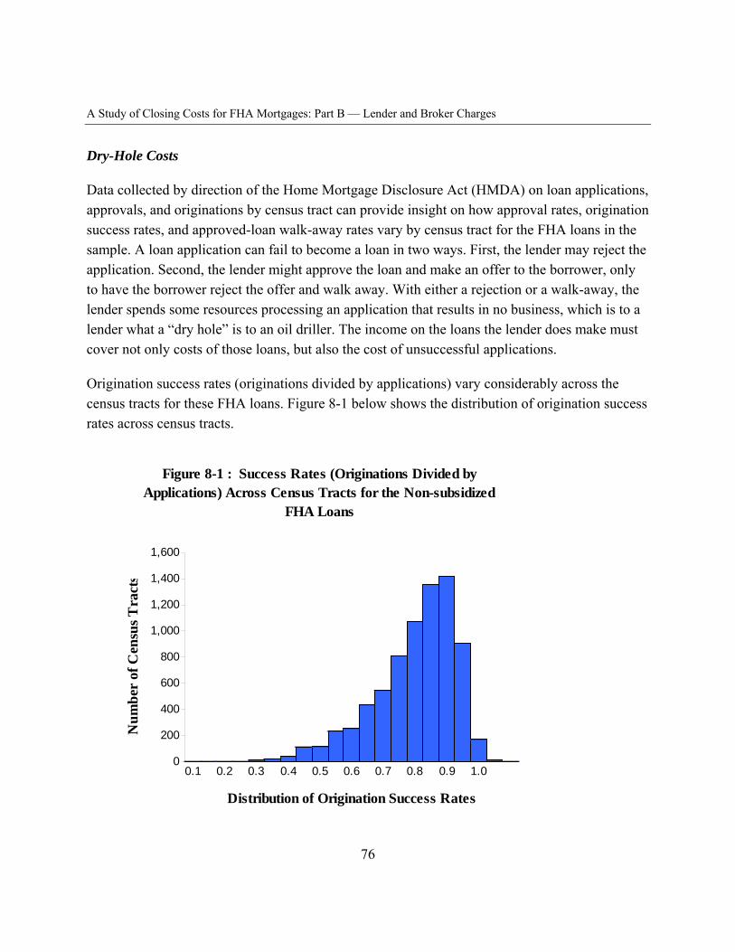
A Study of Closing Costs for FHA Mortgages: Part B — Lender and Broker Charges
Num
ber
of C
ensu
s Tra
cts
Dry-Hole Costs
Data collected by direction of the Home Mortgage Disclosure Act (HMDA) on loan applications, approvals, and originations by census tract can provide insight on how approval rates, origination success rates, and approved-loan walk-away rates vary by census tract for the FHA loans in the sample. A loan application can fail to become a loan in two ways. First, the lender may reject the application. Second, the lender might approve the loan and make an offer to the borrower, only to have the borrower reject the offer and walk away. With either a rejection or a walk-away, the lender spends some resources processing an application that results in no business, which is to a lender what a “dry hole” is to an oil driller. The income on the loans the lender does make must cover not only costs of those loans, but also the cost of unsuccessful applications.
Origination success rates (originations divided by applications) vary considerably across the census tracts for these FHA loans. Figure 8-1 below shows the distribution of origination success rates across census tracts.
Figure 8-1 : Success Rates (Originations Divided by Applications) Across Census Tracts for the Non-subsidized
FHA Loans
1,600
1,400
1,200
1,000
800
600
400
200
0 0.1 0.2 0.3 0.4 0.5 0.6 0.7 0.8 0.9 1.0
Distribution of Origination Success Rates
76
A Study of Closing Costs for FHA Mortgages: Part B — Lender and Broker Charges
Origination success rates are higher for larger loans, higher census tract median income, and higher credit scores, and sharply higher for census tracts with higher levels of education. Success rates are lower in neighborhoods with higher fractions of minority residents, both African Americans and Latinos. Regressions showing the relation between origination success rates and loan and borrower characteristics appear in models 1 through 3 in table 14 of appendix I.
The pattern seen in origination success rates is not driven mainly by approvals, but instead by whether borrowers, if approved, make a deal or walk away. Approval rates rise slightly with loan value, census tract income levels, and census tract education levels. Approval rates are higher when values of owner-occupied houses in the borrower’s census tract are lower. Approval rates are slightly higher, other things equal, for borrowers lacking a credit score. Approval rates are unrelated to the level of credit scores and to neighborhood racial composition. Yet overall, the explanatory power of the approval-rate model is low: this is what should be expected if lenders adjust prices to address differences in expected default and other costs they may incur rather than having a uniform cut-off for the level of tolerable default risk, subject to FHA’s minimum standard of default risk specified in the FHA underwriting guidelines. It appears that FHA lenders do not “red line,” rejecting applications for areas with higher-risk borrowers, but mainly adjust pricing instead.
If origination success is driven mainly by walk-away rates, not rejections, to what factors are walk-away rates related? Walk-away rates are slightly lower in census tracts with higher median incomes but lower for borrowers with larger loans and higher credit scores, and sharply lower for census tracts with higher education levels. The average walk-away rate in census tracts for all nonsubsidized loans is 21 percent, and the average fraction of adults who have completed college is 22 percent. The measured relationship between walk-away rates and education level of the census tract indicates that if all adults in the tract had completed college, the walk-away rate would fall to four percent, raising the origination success rate from the average of 72 percent to 92 percent.
Walk-away rates are higher for borrowers who live in neighborhoods with higher fractions of minority residents. The impact of neighborhood minority composition on walk-away rates is highly systematic. The regressions supporting these measurements appear in models 1 through 3 in table 14 in Appendix I. Note that the origination success rate equals the loan approval rate minus applicant walk-away rate, and the coefficients reflect this identity.
77
A Study of Closing Costs for FHA Mortgages: Part B — Lender and Broker Charges
How much of the variation in lender’s pricing could come from differences in dry hole rates across neighborhoods? This can be measured by adding the “origination success rate” to the basic model measuring how loan fees relate to loan attributes. The first step is to measure the cost of dry holes for lenders. Figure 8-1 above shows that neighborhoods in the sample have origination success rates mainly between 35 percent and 95 percent. The success-rate variable works as follows: in a neighborhood where nearly all applications become loans, lenders do not need to add much to average charges to cover the costs of unsuccessful applications. In a neighborhood where the success rate is low, lenders need to add something. The data contain no information on application fees for loans that do not become originations. However, every closed loan has either an explicit or implicit application charge for processing the application. By regressing loan charges on success rate (plus other variables in the standard model), this relationship is measured statistically. The interpretation of the coefficient on “success rate” is that if the success rate were zero, lenders would cover costs only by charging an application fee of the amount of the estimated coefficient, with sign reversed. The coefficient on success rate thus tells us what the lender will charge if the expected success rate is zero, or simply to process an application; this is the measure of dry-hole cost.
Adding “origination success rate” to the basic regression of total lender/broker charges on loan and borrower characteristics, using only nonsubsidized, direct-lender loans, yields measures of the dry-hole cost of about $120 (t = 0.59). Because education strongly influences success rate but is unrelated to defaults, it is also informative to exclude education from the regression in order to allow “success rate” to account for as much variation as it can, including whatever variation is related to education. This gives an estimate of $410 (t = 2.2) for dry-hole costs.1 It seems reasonable to infer that the dry-hole cost of a mortgage loan is somewhere in the range of $120 to $410.
The regressions are run separately for direct lenders and brokers because broker pricing may reflect the broker’s, but not the wholesale lender’s, dry-hole costs, and because brokers are sufficiently mobile that it may not be possible to make any inference from census tract–level data. For brokers, no dry-hole cost can be detected. The measurements for dry-hole costs appear in models 1 through 3 in table 15a and 15b in appendix I.
Restricting the analysis to loans with coupon rates above seven percent yields similar measures of dry-hole costs. The range is from $77 to $392 for direct lenders.
78
A Study of Closing Costs for FHA Mortgages: Part B — Lender and Broker Charges
Can dry-hole costs account for how much less lenders charge borrowers in neighborhoods with higher levels of education? Not even close. The predicted origination success rate is 0.92 for census tracts where all adults have a college education but loan and borrower characteristics are otherwise average; the success rate is 0.67 in tracts where none do, also other characteristics average. Thus, dry-hole rates would be 25 percentage points lower (0.92 – 0.67) in neighborhoods where all adults have a college education than in those where none do, other things equal. Using the higher estimate ($410) of dry-hole cost, the differences in dry-hole costs can account for roughly $100 (computed as the regression coefficient on BA in the origination success equation (model 3 in table 14 in appendix I), 0.25 x $410 = $103) of the nearly $1,100 bargain enjoyed by borrowers in tracts with higher education levels..
Can dry-hole costs account for race differences in loan charges? Borrowers in neighborhoods that are entirely African American have walk-away rates seven percent higher than those of other borrowers. The average African American FHA borrower in the data lives in a neighborhood that is 47 percent African American as compared with seven percent for the average non-Latino white borrower. Taking again the higher estimate of dry hole costs, $410, multiply first by 0.40 (for difference in percent of neighborhood that is African American between African Americans and non-Latino whites) and then by 0.07 (for the difference in dry-hole rates), and the result is about $11. This is tiny compared to the unexplained premium of roughly $400 paid by African American borrowers.
A similar computation for Latino borrowers, whose walk-away rates are five percent higher than for non-minorities and whose neighborhoods are on average 28 percent Latino as compared with seven percent for non-Latino white borrowers, finds the differential dry-hole cost is about $4, again small compared to the unexplained premium of $365 paid by Latino borrowers.
Table 8-1 below shows the rates for loan approval rates, walk-away rates, and origination success rates, plus dry-hole costs and loan charge differentials for neighborhoods in which all adults have a college education versus those where none do, predicted from the regression measurements.
79
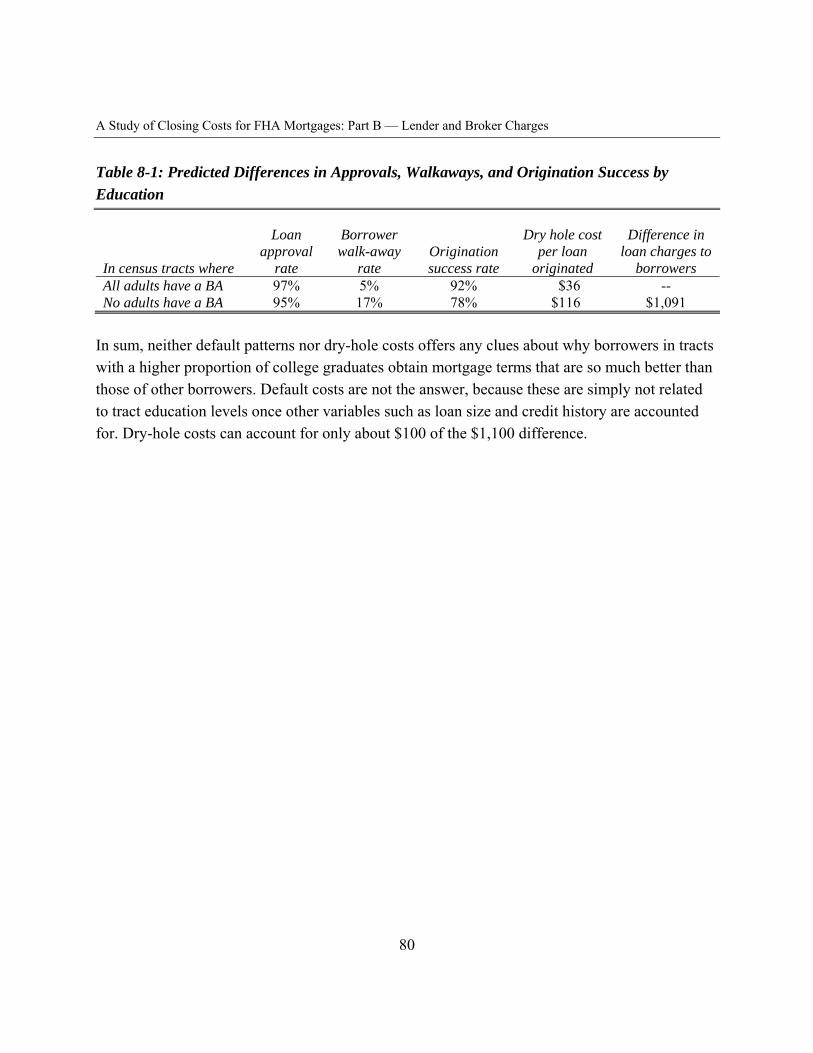
--
A Study of Closing Costs for FHA Mortgages: Part B — Lender and Broker Charges
Table 8-1: Predicted Differences in Approvals, Walkaways, and Origination Success by Education
Loan Borrower Dry hole cost Difference in approval walk-away Origination per loan loan charges to
In census tracts where rate rate success rate originated borrowers All adults have a BA 97% 5% 92% $36 No adults have a BA 95% 17% 78% $116 $1,091
In sum, neither default patterns nor dry-hole costs offers any clues about why borrowers in tracts with a higher proportion of college graduates obtain mortgage terms that are so much better than those of other borrowers. Default costs are not the answer, because these are simply not related to tract education levels once other variables such as loan size and credit history are accounted for. Dry-hole costs can account for only about $100 of the $1,100 difference.
80
A Study of Closing Costs for FHA Mortgages: Part B — Lender and Broker Charges
Chapter IX: Reflections on the Findings
The pattern of origination success rates in relation to borrower education and race suggests a potential dynamic that can account for the differences in charges by education and race.
Lenders and brokers are professionals, and they always know what competitive loan terms are. They have the rate sheets to help them. They also appear to have views regarding how well-informed potential customers are about market prices.,
To the expected-to-be-well-informed borrowers in more educated census tracts, lenders offer better terms. These offers are accepted with high frequency. In these neighborhoods, lenders have low walk-away rates and low dry-hole costs. The measurements indicate that in a hypothetical census tract where all borrowers are white and all adults completed college, lenders will have high success rates, 95 percent. Only two percent of applications are rejected, and only three percent walk away.
To the customers they expect to be less informed, and whose market views are expected to show greater variation, lenders make higher-priced offers. Sometimes these offers are accepted, sometimes the borrowers walk away. The profit from the customers who accept high prices is far above the extra dry-hole costs resulting from some walking away. In the neighborhoods where FHA minority borrowers live, only 4 percent of applications are rejected, 24 percent of the borrowers applied but walked away after being approved, leaving lenders with a success rate of only 72 percent. This suggests that the failure of minorities to obtain terms as good as those of non-minorities is not simply a result of failure to shop. Nearly a quarter of them get a quote and reject it.
If some of the expected-to-be less-informed borrowers are actually well informed, but assign a higher personal cost to another loan application (perhaps because they are members of a group that has been ill treated by credit markets historically), they too may accept inferior terms to avoid another application. The strategy of offering worse terms to minorities who are especially averse to the application process will result in higher walkaways but still be profitable to lenders. Perversely, the strategy of quoting high prices to minority borrowers also forces many to reapply elsewhere, despite their distaste for this process.
Price discrimination of this type does not arise in competitive markets with informed shoppers. Even a truly inelastic demander (that is, someone more willing to pay higher prices, such as a
81
A Study of Closing Costs for FHA Mortgages: Part B — Lender and Broker Charges
minority borrower who is especially averse to loan rejection) should be able to easily find and get the competitive price in a competitive market. For price discrimination to be possible, there must be some friction—some inhibition to competition such as a high transaction or search cost or some limitation on information that makes it difficult for one side of the market (borrowers) to see all available prices. The auto markets and auto lending markets, like the mortgage markets, are characterized by many sellers and easy market entry for sellers (traditionally, the presumed requirements for a competitive market). Yet price discrimination is found in these markets also. Evidently the buyer’s informational disadvantage plus some friction from the cost of shopping allows sellers to offer, and receive, higher prices from some customers. The mortgage market appears to suffer from similar frictions.
In full equilibrium, however, the competition among lenders and brokers to find and woo these high-paying customers would result in them spending more resources pursuing these customers. The additional resources (including time) spent seeking high-paying customers would drive the average profit even on these more expensive loans to zero. This is not an efficient equilibrium from a social point of view. The lender/broker gets a higher price and the borrower pays a higher price, but no one is better off, not even the lender/broker, because the lender/broker spends more resources to get the high-paying customers. Thus, the additional effort spent by the lender/broker is, from a social point of view, wasted resources.
Another inference that can be drawn from the pattern of prices and success rates in this study is that differences in the terms offered to minorities and to less-educated borrowers must be even larger than the differences seen here in prices that are accepted. The logic is as follows: first, it seems reasonable that the terms borrowers accept are, on average, better than those that are rejected. For borrowers with high education levels, the data reveal a large fraction of the offers made because such a large fraction is accepted. For these borrowers, the difference between accepted offers and all offers must be small. For minority and less-educated borrowers, the walkaway rates are higher, and the prices (interest rates and cash fees) on these offers are higher than those seen among the loans actually made. The difference between accepted offers and all offers must be larger. It follows that the differences in all terms offered must be larger than the differences seen in terms accepted.
If this interpretation of the dynamics of the mortgage market is correct, it is unlikely that additional data on factors related to default risk—for example, more detailed credit or employment history—will “explain away” the race and education differences. It is possible that survey findings such as those done by Scott Morton, Zettelmeyer, and Silva-Risso (2005) and by
82
A Study of Closing Costs for FHA Mortgages: Part B — Lender and Broker Charges
Courchane, Surette and Zorn (2003) investigating which borrowers like or dislike negotiation, shopping, and researching prices could offer some insight. Of course such results would still beg the question as to why some customers are eager to engage the market while others are not. The answer may lie in how they and others like them have been treated by markets both in history and in legend, and the resulting self-confidence with which they approach the problem of finding a mortgage loan.
An important question is how much improved loan disclosures, especially at the time of loan application, could help borrowers who have not spent so many years in school or who were born into minority families. The results on how borrower education and race are related to origination success rates in chapter VIII, plus the findings on no-cost loans in chapter VII—almost no education premium, little difference by race, and much lower prices—on the no-cost loans, suggest that better information can be part of the solution.
The study done by James Lacko and Janis Pappalardo of the Federal Trade Commission, published in summer 2007, confirms that our existing mortgage disclosures are not very effective and demonstrates that improved disclosures are possible. As big an improvement as the FTC’s revised disclosures are, the research on better disclosures should not stop there. The FTC studied one variation on improved disclosures. As was learned with the development of the FDA’s nutrition label, designing an effective disclosure is not easy, and it cannot be done from first principles. One must design a disclosure and test it, revise and improve it, and test it again, and it is likely that many revisions will produce improvements. Type face matters, type size matters, and white space matters, as do boxes and other design features that guide a reader’s eye to the most important figures. With a few more resources for research, it is likely that a disclosure even better than the FTC’s new version can be developed.
One issue that will arise in disclosure design is the benefit of disclosing a yield-spread premium to borrowers. This study cannot speak to that issue. The YSP is disclosed on brokered loans but not on loans made by direct lenders. Yet brokered loans are on average more expensive than direct loans—indeed, they are the most expensive of the four types of lenders studied here. Would brokered loans be even more expensive if the YSP were not disclosed?
The way the YSP is disclosed at present is surely poor. Many borrowers do not see a YSP until their loan closing, many will not see it even then among the many figures on the typical HUD-1 settlement statement. If they do see it, most borrowers are reluctant to do anything that would jeopardize their loan closing. In addition, in the only research that compares disclosed YSPs to
83
A Study of Closing Costs for FHA Mortgages: Part B — Lender and Broker Charges
those from lender’s electronic records (Woodward 2003, for a set of brokered loans that originated from 1996 to 2001), one-third of YSPs were missing from HUD-1s, and the relation between disclosed YSP and the YSP in the wholesale lender’s records was far from perfect. Whether the YSP was present on the HUD-1 was unrelated to how much borrowers were charged.
One might think, given this study’s emphasis on up-front cash charges plus a YSP, that these two figures are sufficient information for borrowers to choose a loan. That inference is wrong. In the computations for this study, the cost adjustments per dollar of loan amount were the same for all loans at the same coupon rate. This condition does not prevail out there in the real world.
For example, suppose a borrower got two quotes with identical up-front cash charges and identical interest rates but different YSPs. The loans are of equal cost, period. To add the cash costs and YSP and choose the loan with the lower total would not do the borrower any harm because the costs are the same, but it would not create any benefit either.
But suppose instead that a borrower gets a quote one week, then another a few weeks later, at which point interest rates have risen a little. The second quote will likely have a higher rate but it might have the same, or a lower, or a higher YSP. Choosing the loan with the lower total cash plus YSP could lead the borrower wrong. Unlike the computations in this study, these two loans would not have YSP differences that equated interest differentials.
A large YSP on either a good-faith estimate or a HUD-1 might alert a borrower that the compensation to the broker is high, and a better deal might be found elsewhere. The author has heard personal accounts of very-well-educated borrowers with large loans seeing a large YSP on the HUD-1, at closing, and from this inferring that they were not getting such a great deal. But these are anecdotes. Data is the plural of anecdote,1 and data should inform the design of our disclosure forms.
Whether and how much disclosure of the YSP, in addition to other information, could help borrowers choose their mortgages better is an empirical question, one that can only be answered with data produced by testing. Decisions regarding what to disclose and how to disclose it should not be left to lawyers and economists, no matter how good-hearted they are. Broader social science skills should be brought to the problem.
84
A Study of Closing Costs for FHA Mortgages: Part B — Lender and Broker Charges
The engineers who design jet aircraft do not design the displays or controls pilots use to control the aircraft. Instead, social and industrial psychologists get involved; they test designs to see what kinds of mistakes pilots make, try to understand why pilots make them, and revise displays and controls to avoid mistakes. Why should our financial disclosures be different? The same skills addressing comprehension and cognition should inform financial disclosures for consumers. There should be no more disclosure rules written without research to determine whether borrowers notice, understand, and make correct inferences from the disclosures. This of course implies no more financial disclosure rules without a serious effort at disclosure design.
85

A Study of Closing Costs for FHA Mortgages: Part C — Title Charges and Real Estate Transaction Fees
PART C: TITLE CHARGES AND REAL ESTATE TRANSACTION FEES
Chapter X: Title Charges
Title charges are a substantial part of the cost of obtaining a home mortgage. For the nonsubsidized loans studied here, title charges average $1,200 per loan, just a bit lower than the average of $1,300 cash paid to lender/brokers, and close to half the average borrower’s down payment of $2,500.
Controversies in Title Insurance
Title charges have been a controversial aspect of settlement services for many decades. They have been the focus of federal and state litigation, government investigations, and such reports as the U.S. Government Accountability Office report of April 2007 and Birnbaum’s Report to the California Insurance Commissioner in December 2005. The data collected for this study offer a rare opportunity to analyze actual amounts paid by borrowers for title services and thus to inform this controversy in a new way.
Two views of title services emerge from the long commentary on the title services business. The primary difference in these views concerns the role of referral fees, kickbacks, or rebates from title agencies to lender/brokers and/or real estate agents. One view, associated with economists Bruce Owen (1977) and Lawrence White (1984), is that title companies are able to tacitly collude (with more than a little help from state regulation) to charge prices for title services that are well above cost. Economists refer to the difference between price and cost as profit or “economic rent.” (“Cost” includes a competitive return on capital.) They contend that as a result of the large profit—the margin between price and cost—title companies compete to generate additional business by offering kickbacks or rebates to those in a position to bring customers to them, typically either real estate agents or lenders and mortgage brokers.
Economists cite the following as reasons to suspect that title charges are above competitive levels:
1. Title charges generally are positively correlated with property values. (The scatter plots of title charges against property value provided in appendix V show this clearly.) The cost of providing title services is mainly the effort involved in the title search, which is the same for high- and low-value properties. Thus, if charges reflected cost, which is to
86
A Study of Closing Costs for FHA Mortgages: Part C — Title Charges and Real Estate Transaction Fees
be expected in a competitive market, charges would be at most slightly related to property values. A positive relation between charges and loan amounts or property values implies price discrimination, and this is evidence of a noncompetitive market.
2. The profitability of title services at all levels is high. (See appendix IV for details.)
3. Market concentration in title services is high and has been rising over the past several decades as large title companies buy smaller ones. (Details are in appendix IV.)
Owen (1977) and White (1984) contend that in equilibrium, with no regulatory interference in the payment of kickbacks and rebates, market forces will cause the payments from title companies to real estate agents or lender/brokers to rise until the profit to the title service companies reaches zero. With each transaction bringing revenue from title referrals, real estate agents and lender/brokers will compete in lowering their own prices to consumers, ultimately resulting in competitive prices overall for the package of settlement services (either realty service plus title or loan plus title). In this view, the Real Estate Settlement Procedures Act, by prohibiting referral fees and kickbacks, prevents competition from eliminating the cartel profits in title insurance by inhibiting competition’s ability to work through real estate agents and lenders bundling their own services with title services.
In the alternative view, that of the title service industry, real estate agents and lenders, who are the first to meet customers who need title services, pressure title companies for referral fees or kickbacks when they refer customers to them. Referral fees become a cost of doing business to the title agencies, causing them to raise their prices to cover these costs. This is often referred to as “reverse competition.”
Essentially, in the economists’ view, high prices “cause” referral fees and kickbacks by placing a wedge between price and cost, making referrals valuable and inducing title agencies to offer referral fees and kickbacks to those who will bring them customers. In the industry view, kickbacks and referral fees “cause” high prices by raising costs to title agencies through the “reverse competition” for customer referrals.
The cartel pricing hypothesis for title services is consistent with what happened after the passage of RESPA in 1975. RESPA prohibits referral fees, kickbacks, and rebates among providers of settlement services except for those paid between real estate agents and from title insurance companies to their title insurance agents. After 1975, many lenders and real estate agencies sought to acquire whole or partial ownership of title service agencies. These relationships were
87
A Study of Closing Costs for FHA Mortgages: Part C — Title Charges and Real Estate Transaction Fees
referred to by the title service providers as “controlled business arrangements” or, later, “affiliated business arrangements.” The motivation for entering such arrangements is for a single organization (which would include a title agency and either a lender/broker or real estate agent) to be able to collect the profit of its affiliated title business without an explicit kickback or rebate. In reaction to this movement, the title service business lobbied for and secured amendments to RESPA in 1983 that restricted “controlled business” or “affiliated business” arrangements.
If RESPA obstructed competitive pricing of title services for consumers on real estate settlements by prohibiting lenders and/or real estate agents from bundling and pricing their services along with title services, then the 1983 amendments to RESPA likely do so as well. They preclude another avenue by which the profits in title services might be competed away.
What the Data Reveal
Title charges are analyzed here by the same approach that lender/broker fees were analyzed earlier—that is, by asking to what loan and borrower characteristics these fees are related.
Here “title charges” include all the fees that are intended to appear in the “1100” series (lines) of the HUD-1 settlement statement. This is the sum of title insurance premiums, other charges related to obtaining a title insurance policy such as searches and abstracts, and courier fees and other services performed or arranged by the party who conducts the closing (the meeting at which final loan and sale papers are signed), often referred to as the closing agent, settlement agent, escrow agent, or title agent or company. The focus is on the sum of all payments for title services, including legal services, for four reasons. First, the fees appearing in the 1100s are mainly determined by the title, escrow, settlement or closing agent. Second, most (roughly 80 percent) of the title insurance premium is ultimately compensation to the title agent.1 Third, when attorney services are required, it appears they displace other title services (discussed later). Finally, the different fees for title services, like broker/lender fees, appear arbitrary in how they are described and how they are broken down into sub-fees and are thus best analyzed as a sum. In any case, it is difficult to tell from HUD-1 settlement statements what amounts are paid for insurance versus other services, such as research to identify and resolve title issues before closing. Amounts appearing in the 1100 series that were clearly not payments for title services (such as property taxes due, sales taxes on title charges, or payments for such services as pest control or gardening) were not included in title charges.
The five main findings are as follows:
88
A Study of Closing Costs for FHA Mortgages: Part C — Title Charges and Real Estate Transaction Fees
1. On average, title charges rise with loan amount. How strongly title charges relate to loan amount varies by state. In some states the relationship is strong, while in others title fees and loan amount are not at all related. Given that the cost of providing title services has at most a weak relation to loan amount or property value (because payouts on policies are so rare), this finding supports the hypothesis of widespread price discrimination in title services and an absence of effective competition in states where title fees rise with loan amount. The three most expensive states for title fees (after taking account of loan and borrower variations)—New York, California, and Texas—are three of the top four states where title fees rise fastest with loan amount.
2. Title charges show other signs of price discrimination related to race and education; homebuyers in tracts with more minorities and fewer college graduates pay more. Given the absence of any reason race or education should relate to the cost of establishing or resolving title for a property, this appears to be straightforward price discrimination, again suggesting a less-than-competitive market.
3. A large fraction (nearly 25 percent) of the variance in how much borrowers are charged for title services relates to the state in which the borrower lives. It seems implausible that the cost of researching a title can vary this much across States, or that it could vary in the pattern seen—related to loan amount in some states, but not in others, and more systematically connected to loan amount in states with large populations. This suggests that the success of attempts at cartel pricing varies at the state level. The most expensive title services are in the states with the largest populations—California, Texas, New York, and Florida. North Carolina and Georgia are outliers; they are among the 10 most populous states but among the 5 lowest states for title costs.
4. How much borrowers are charged for title services rises with the fees charged by lender/brokers and by real estate agents. Elevated fees are present even after taking account of all the other usual loan and borrower characteristics. This finding suggests a reason, not previously discussed, for why kickbacks and referral fees are such a big issue in title fees: when a real estate agent or lender refers a customer to a title agent, the title agent makes not only the usual profit, but also an additional profit related to the customer’s apparent vulnerability to paying additional fees.
5. After all these factors are identified and measured, there is still substantial unexplained variation in title fees even within individual states and within given ranges for loan amount. With lender/broker fees, complex items such as YSPs, discount points, and seller
89
A Study of Closing Costs for FHA Mortgages: Part C — Title Charges and Real Estate Transaction Fees
contributions helped identify how borrower confusion contributed to high charges to borrowers. For title fees, there are no similar items to explore.
In sum, without state indicators, just under 40 percent of the variation in charges for title services relates to loan and borrower characteristics, including how much borrowers paid to lender/brokers and real estate agents. While median area income may reflect local wage levels (and thus relate to the cost of providing title services), and the true insurance aspect of title services may weakly relate to loan amount, it appears that much of the variation in title charges is simple price discrimination related to race, education, and ability to pay. Adding the states in which the borrowers live as categorical variables raises the fraction of variance related to loan and borrower characteristics to just over 60 percent.
Variations among and within States
Variation in title charges from one state to another is larger than is the state variation in lender/broker fees. As seen below in table 10-1, average title charges by state range from $668 to $2,090. Twelve states average title charges of less than $900, while five average over $1,700
Table 10-1 shows how title fees are related to loan amount, down payment, (estimated or predicted) yield spread premiums, cash loan origination fees, and realty fees for each state. In thirty-three states, title fees rise with loan amount and the rate at which they rise is estimated with sufficient precision to leave little doubt that this relationship is systematic. (the coefficient is at least double its standard error). In eleven states, title fees rise with the fees paid to the real estate agent, and in eleven states, title fees rise with at least one type of lender compensation (YSP or cash fees). The neighborhood racial composition and education measures were omitted from these state-level regressions because there are a few small states with essentially no minority borrowers in the FHA sample.
How much do title fees vary by state after taking account of loan and borrower characteristics? Table 10-2 shows the amount by which each state’s fees are elevated after taking account of loan and borrower characteristics compared to the state with the lowest title charges (other things equal), North Carolina. These figures are the coefficients on individual state categorical (dummy) variables from a regression that includes all of the other standard loan and borrower characteristics. These differences in state title charges are, to a very limited degree, related to different categories of title regulation identified and discussed in Appendix IV (see model 3 in table 16 in appendix I). In the highest cost states, New York, Texas, California, and New Jersey,
90
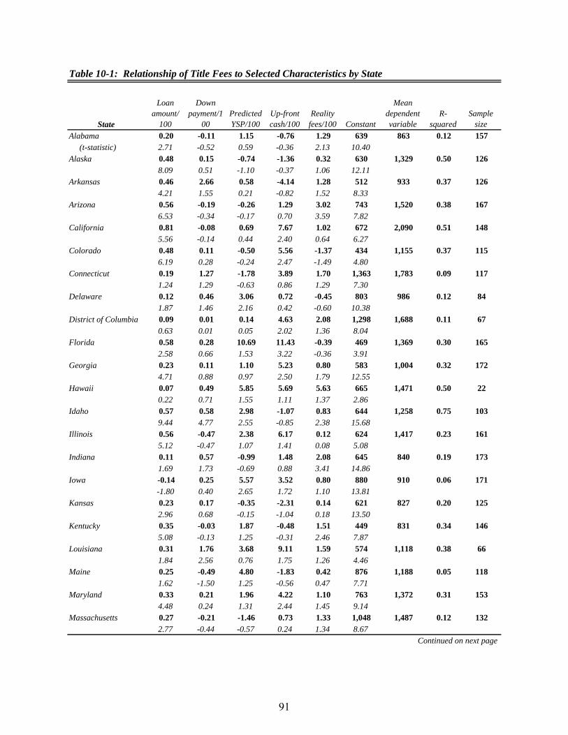
Table 10-1: Relationship of Title Fees to Selected Characteristics by State
Loan Down Mean amount/ payment/1 Predicted Up-front Reality dependent R- Sample
State 100 00 YSP/100 cash/100 fees/100 Constant variable squared size Alabama 0.20 -0.11 1.15 -0.76 1.29 639 863 0.12 157
(t-statistic) 2.71 -0.52 0.59 -0.36 2.13 10.40 Alaska 0.48 0.15 -0.74 -1.36 0.32 630 1,329 0.50 126
8.09 0.51 -1.10 -0.37 1.06 12.11 Arkansas 0.46 2.66 0.58 -4.14 1.28 512 933 0.37 126
4.21 1.55 0.21 -0.82 1.52 8.33 Arizona 0.56 -0.19 -0.26 1.29 3.02 743 1,520 0.38 167
6.53 -0.34 -0.17 0.70 3.59 7.82 California 0.81 -0.08 0.69 7.67 1.02 672 2,090 0.51 148
5.56 -0.14 0.44 2.40 0.64 6.27 Colorado 0.48 0.11 -0.50 5.56 -1.37 434 1,155 0.37 115
6.19 0.28 -0.24 2.47 -1.49 4.80 Connecticut 0.19 1.27 -1.78 3.89 1.70 1,363 1,783 0.09 117
1.24 1.29 -0.63 0.86 1.29 7.30 Delaware 0.12 0.46 3.06 0.72 -0.45 803 986 0.12 84
1.87 1.46 2.16 0.42 -0.60 10.38 District of Columbia 0.09 0.01 0.14 4.63 2.08 1,298 1,688 0.11 67
0.63 0.01 0.05 2.02 1.36 8.04 Florida 0.58 0.28 10.69 11.43 -0.39 469 1,369 0.30 165
2.58 0.66 1.53 3.22 -0.36 3.91 Georgia 0.23 0.11 1.10 5.23 0.80 583 1,004 0.32 172
4.71 0.88 0.97 2.50 1.79 12.55 Hawaii 0.07 0.49 5.85 5.69 5.63 665 1,471 0.50 22
0.22 0.71 1.55 1.11 1.37 2.86 Idaho 0.57 0.58 2.98 -1.07 0.83 644 1,258 0.75 103
9.44 4.77 2.55 -0.85 2.38 15.68 Illinois 0.56 -0.47 2.38 6.17 0.12 624 1,417 0.23 161
5.12 -0.47 1.07 1.41 0.08 5.08 Indiana 0.11 0.57 -0.99 1.48 2.08 645 840 0.19 173
1.69 1.73 -0.69 0.88 3.41 14.86 Iowa -0.14 0.25 5.57 3.52 0.80 880 910 0.06 171
-1.80 0.40 2.65 1.72 1.10 13.81 Kansas 0.23 0.17 -0.35 -2.31 0.14 621 827 0.20 125
2.96 0.68 -0.15 -1.04 0.18 13.50 Kentucky 0.35 -0.03 1.87 -0.48 1.51 449 831 0.34 146
5.08 -0.13 1.25 -0.31 2.46 7.87 Louisiana 0.31 1.76 3.68 9.11 1.59 574 1,118 0.38 66
1.84 2.56 0.76 1.75 1.26 4.46 Maine 0.25 -0.49 4.80 -1.83 0.42 876 1,188 0.05 118
1.62 -1.50 1.25 -0.56 0.47 7.71 Maryland 0.33 0.21 1.96 4.22 1.10 763 1,372 0.31 153
4.48 0.24 1.31 2.44 1.45 9.14 Massachusetts 0.27 -0.21 -1.46 0.73 1.33 1,048 1,487 0.12 132
2.77 -0.44 -0.57 0.24 1.34 8.67 Continued on next page
91
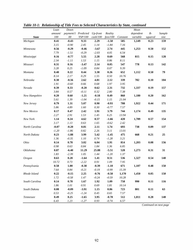
Table 10-1: Relationship of Title Fees to Selected Characteristics by State, continued Loan Down Mean
amount/ payment/1 Predicted Up-front Reality dependent R- Sample State 100 00 YSP/100 cash/100 fees/100 Constant variable squared size
Michigan 0.41 -0.43 9.33 2.29 -1.50 585 1,149 0.23 159 3.15 -0.90 2.45 1.14 -1.84 7.16
Minnesota 0.56 -0.29 -0.46 -3.67 2.74 445 1,253 0.50 152 7.79 -1.51 -0.29 -2.03 4.05 6.54
Mississippi 0.16 -0.77 5.55 2.28 0.69 568 815 0.15 128 2.34 -1.11 1.53 1.15 0.86 8.11
Missouri 0.31 0.16 -3.47 2.14 0.05 547 778 0.13 142 3.28 0.25 -1.09 0.84 0.07 9.39
Montana 0.40 0.22 0.44 3.38 0.26 652 1,112 0.50 79 8.14 2.17 0.29 1.55 0.50 10.76
Nebraska 0.30 -0.56 2.62 4.81 2.12 339 782 0.10 104 1.91 -0.60 0.66 0.68 1.97 3.95
Nevada 0.39 0.33 -0.20 0.62 2.31 732 1,337 0.19 157 3.84 0.57 -0.11 0.32 2.80 7.38
New Hampshire 0.20 0.60 -1.21 -0.18 0.49 860 1,180 0.20 162 5.61 1.39 -1.04 -0.15 1.15 21.04
New Jersey 0.79 1.31 5.07 0.90 -0.93 788 1,922 0.44 171 5.86 4.89 1.60 0.30 -0.77 7.57
New Mexico 0.17 0.47 2.42 1.91 3.79 744 1,174 0.49 135 2.27 2.91 1.53 1.45 6.25 13.94
New York 1.14 0.24 4.62 8.57 -1.66 420 1,789 0.57 154 3.17 1.13 0.63 1.65 -0.62 2.42
North Carolina -0.07 -0.20 0.81 2.11 1.74 693 738 0.09 137 -1.20 -1.86 0.82 2.26 3.11 13.01
North Dakota 0.23 -1.88 3.99 5.42 -1.45 475 668 0.21 25 1.36 -0.35 1.10 0.74 -1.28 3.21
Ohio 0.14 0.78 3.02 6.04 1.91 814 1,203 0.08 156 0.98 0.63 0.84 1.84 1.36 6.85
Oklahoma 0.87 -6.40 11.29 25.88 -5.51 528 1,273 0.31 31 1.83 -2.39 1.05 1.44 -1.20 1.37
Oregon 0.63 0.28 -1.64 1.41 0.51 536 1,327 0.54 140 10.72 0.73 -2.22 0.91 1.09 7.95
Pennsylvania 0.58 1.00 -0.38 -0.39 -1.10 671 1,107 0.48 150 7.64 0.84 -0.21 -0.19 -0.99 15.39
Rhode Island 0.22 -0.15 2.25 -0.76 -0.58 1,170 1,450 0.05 150 1.72 -0.58 1.47 -0.24 -0.59 10.28
South Carolina 0.14 0.78 1.67 1.92 1.09 758 990 0.11 116 1.86 1.01 0.91 0.69 1.81 10.14
South Dakota 0.08 -0.09 -3.91 1.15 0.86 723 801 0.11 63 0.53 -0.25 -1.24 0.45 0.65 7.57
Tennessee 0.49 0.25 -1.65 3.95 -0.78 512 1,011 0.28 148 6.43 1.23 -1.27 0.93 -0.74 6.57
Continued on next page
92
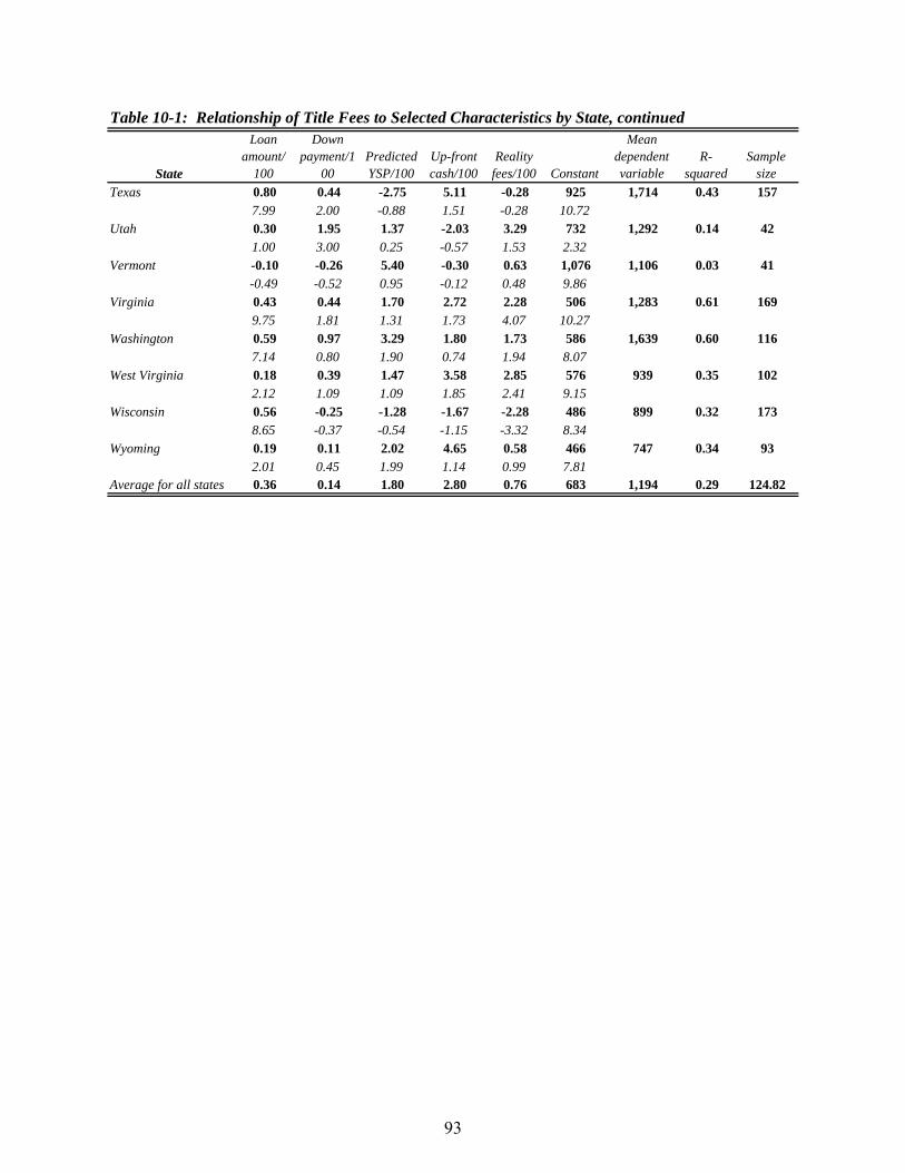
Table 10-1: Relationship of Title Fees to Selected Characteristics by State, continued Loan Down Mean
State Texas
amount/ 100 0.80
payment/1 00
0.44
Predicted YSP/100
-2.75
Up-front cash/100
5.11
Reality fees/100
-0.28 Constant
925
dependent variable
1,714
R-squared
0.43
Sample size 157
7.99 2.00 -0.88 1.51 -0.28 10.72 Utah 0.30 1.95 1.37 -2.03 3.29 732 1,292 0.14 42
1.00 3.00 0.25 -0.57 1.53 2.32 Vermont -0.10 -0.26 5.40 -0.30 0.63 1,076 1,106 0.03 41
-0.49 -0.52 0.95 -0.12 0.48 9.86 Virginia 0.43
9.75 0.44 1.81
1.70 1.31
2.72 1.73
2.28 4.07
506 10.27
1,283 0.61 169
Washington 0.59 7.14
0.97 0.80
3.29 1.90
1.80 0.74
1.73 1.94
586 8.07
1,639 0.60 116
West Virginia 0.18 2.12
0.39 1.09
1.47 1.09
3.58 1.85
2.85 2.41
576 9.15
939 0.35 102
Wisconsin 0.56 -0.25 -1.28 -1.67 -2.28 486 899 0.32 173 8.65 -0.37 -0.54 -1.15 -3.32 8.34
Wyoming 0.19 2.01
0.11 0.45
2.02 1.99
4.65 1.14
0.58 0.99
466 7.81
747 0.34 93
Average for all states 0.36 0.14 1.80 2.80 0.76 683 1,194 0.29 124.82
93
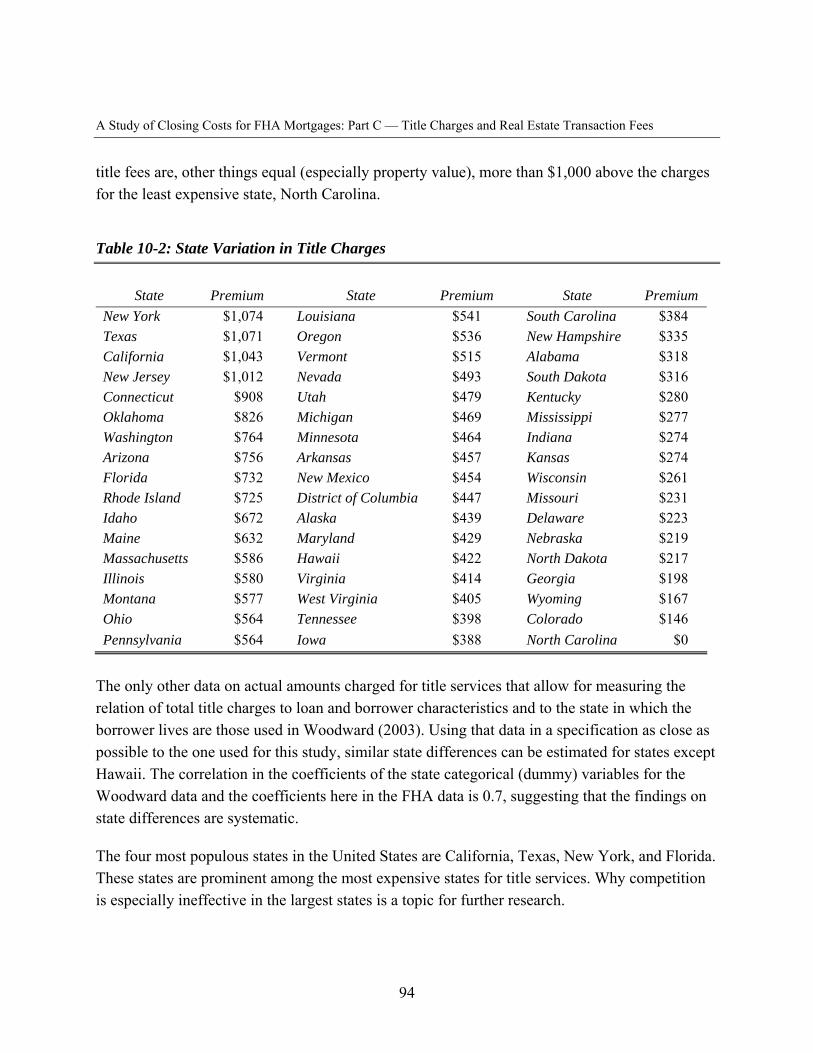
A Study of Closing Costs for FHA Mortgages: Part C — Title Charges and Real Estate Transaction Fees
title fees are, other things equal (especially property value), more than $1,000 above the charges for the least expensive state, North Carolina.
Table 10-2: State Variation in Title Charges
State Premium State Premium State Premium New York $1,074 Louisiana $541 South Carolina $384 Texas $1,071 Oregon $536 New Hampshire $335 California $1,043 Vermont $515 Alabama $318 New Jersey $1,012 Nevada $493 South Dakota $316 Connecticut $908 Utah $479 Kentucky $280 Oklahoma $826 Michigan $469 Mississippi $277 Washington $764 Minnesota $464 Indiana $274 Arizona $756 Arkansas $457 Kansas $274 Florida $732 New Mexico $454 Wisconsin $261 Rhode Island $725 District of Columbia $447 Missouri $231 Idaho $672 Alaska $439 Delaware $223 Maine $632 Maryland $429 Nebraska $219 Massachusetts $586 Hawaii $422 North Dakota $217 Illinois $580 Virginia $414 Georgia $198 Montana $577 West Virginia $405 Wyoming $167 Ohio $564 Tennessee $398 Colorado $146 Pennsylvania $564 Iowa $388 North Carolina $0
The only other data on actual amounts charged for title services that allow for measuring the relation of total title charges to loan and borrower characteristics and to the state in which the borrower lives are those used in Woodward (2003). Using that data in a specification as close as possible to the one used for this study, similar state differences can be estimated for states except Hawaii. The correlation in the coefficients of the state categorical (dummy) variables for the Woodward data and the coefficients here in the FHA data is 0.7, suggesting that the findings on state differences are systematic.
The four most populous states in the United States are California, Texas, New York, and Florida. These states are prominent among the most expensive states for title services. Why competition is especially ineffective in the largest states is a topic for further research.
94
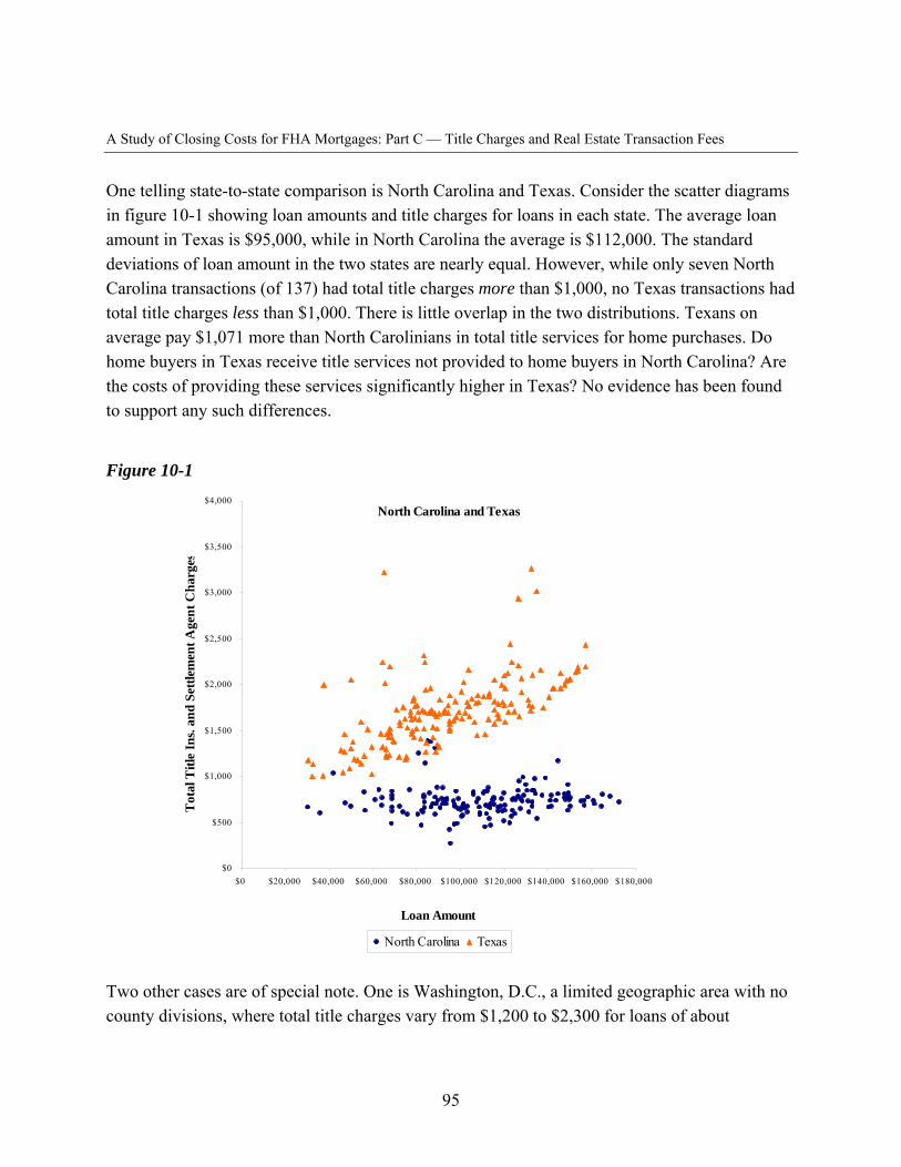
A Study of Closing Costs for FHA Mortgages: Part C — Title Charges and Real Estate Transaction Fees
One telling state-to-state comparison is North Carolina and Texas. Consider the scatter diagrams in figure 10-1 showing loan amounts and title charges for loans in each state. The average loan amount in Texas is $95,000, while in North Carolina the average is $112,000. The standard deviations of loan amount in the two states are nearly equal. However, while only seven North Carolina transactions (of 137) had total title charges more than $1,000, no Texas transactions had total title charges less than $1,000. There is little overlap in the two distributions. Texans on average pay $1,071 more than North Carolinians in total title services for home purchases. Do home buyers in Texas receive title services not provided to home buyers in North Carolina? Are the costs of providing these services significantly higher in Texas? No evidence has been found to support any such differences.
Figure 10-1
Tot
al T
itle
Ins.
and
Settl
emen
t Age
nt C
harg
es
$4,000
$3,500
$3,000
$2,500
$2,000
$1,500
$1,000
$500
$0
North Carolina and Texas
$0 $20,000 $40,000 $60,000 $80,000 $100,000 $120,000 $140,000 $160,000 $180,000
Loan Amount
North Carolina Texas
Two other cases are of special note. One is Washington, D.C., a limited geographic area with no county divisions, where total title charges vary from $1,200 to $2,300 for loans of about
95
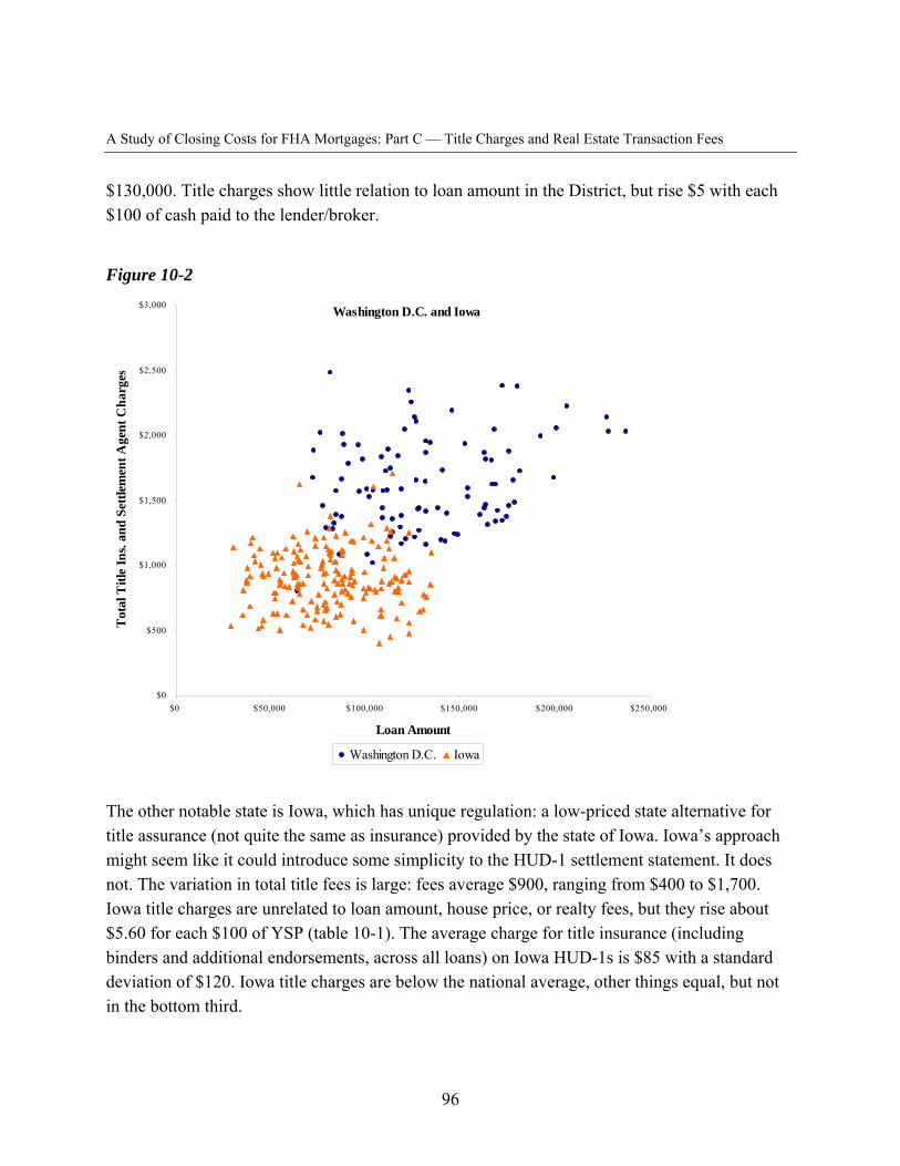
A Study of Closing Costs for FHA Mortgages: Part C — Title Charges and Real Estate Transaction Fees
$130,000. Title charges show little relation to loan amount in the District, but rise $5 with each $100 of cash paid to the lender/broker.
Figure 10-2
Tot
al T
itle
Ins.
and
Settl
emen
t Age
nt C
harg
es
$3,000
$2,500
$2,000
$1,500
$1,000
$500
$0
Washington D.C. and Iowa
$0 $50,000 $100,000 $150,000 $200,000 $250,000
Loan Amount
Washington D.C. Iowa
The other notable state is Iowa, which has unique regulation: a low-priced state alternative for title assurance (not quite the same as insurance) provided by the state of Iowa. Iowa’s approach might seem like it could introduce some simplicity to the HUD-1 settlement statement. It does not. The variation in total title fees is large: fees average $900, ranging from $400 to $1,700. Iowa title charges are unrelated to loan amount, house price, or realty fees, but they rise about $5.60 for each $100 of YSP (table 10-1). The average charge for title insurance (including binders and additional endorsements, across all loans) on Iowa HUD-1s is $85 with a standard deviation of $120. Iowa title charges are below the national average, other things equal, but not in the bottom third.
96
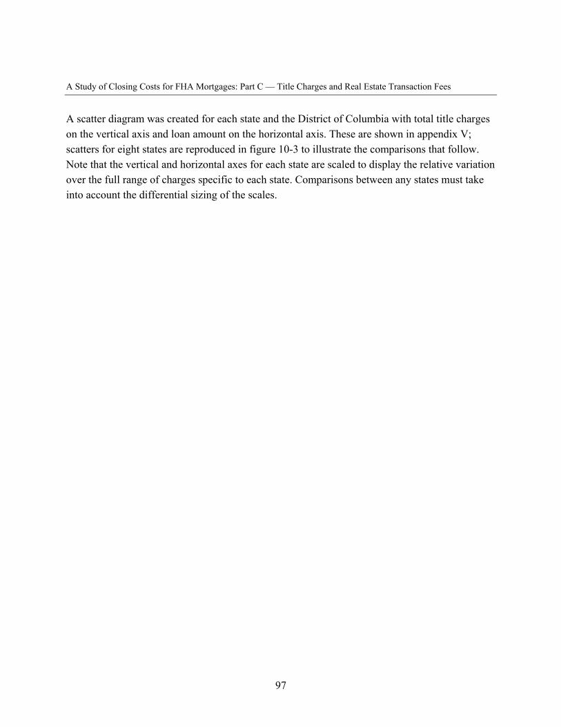
A Study of Closing Costs for FHA Mortgages: Part C — Title Charges and Real Estate Transaction Fees
A scatter diagram was created for each state and the District of Columbia with total title charges on the vertical axis and loan amount on the horizontal axis. These are shown in appendix V; scatters for eight states are reproduced in figure 10-3 to illustrate the comparisons that follow. Note that the vertical and horizontal axes for each state are scaled to display the relative variation over the full range of charges specific to each state. Comparisons between any states must take into account the differential sizing of the scales.
97
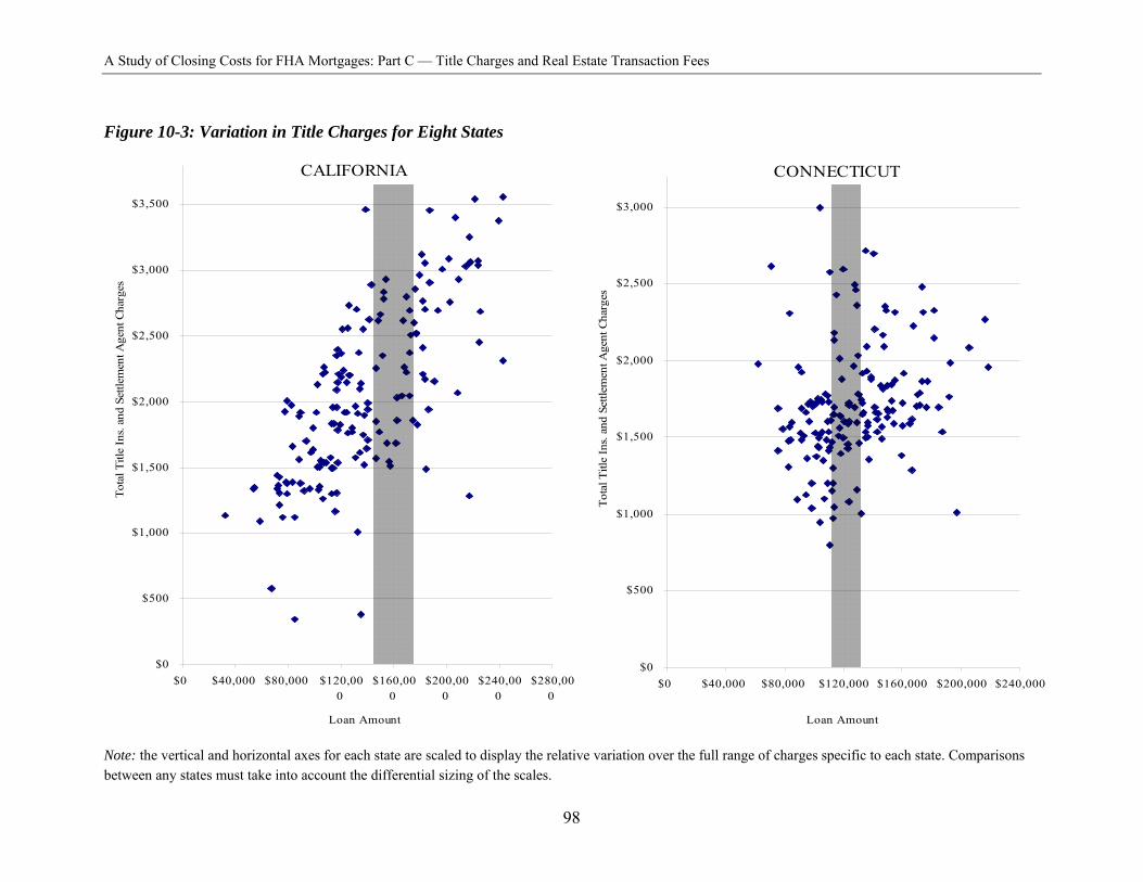
A Study of Closing Costs for FHA Mortgages: Part C — Title Charges and Real Estate Transaction Fees
Figure 10-3: Variation in Title Charges for Eight States
$3,500
CALIFORNIA
$3,000
$3,000 $2,500
CONNECTICUT
Tota
l Titl
e In
s. an
d Se
ttlem
ent A
gent
Cha
rges
Tota
l Titl
e In
s. an
d Se
ttlem
ent A
gent
Cha
rges
$2,500
$2,000
$2,000
$1,500
$1,500
$1,000 $1,000
$500$500
$0 $0 $0 $40,000 $80,000 $120,00 $160,00 $200,00 $240,00 $280,00 $0 $40,000 $80,000 $120,000 $160,000 $200,000 $240,000
0 0 0 0 0
Loan Amount Loan Amount
Note: the vertical and horizontal axes for each state are scaled to display the relative variation over the full range of charges specific to each state. Comparisons between any states must take into account the differential sizing of the scales.
98
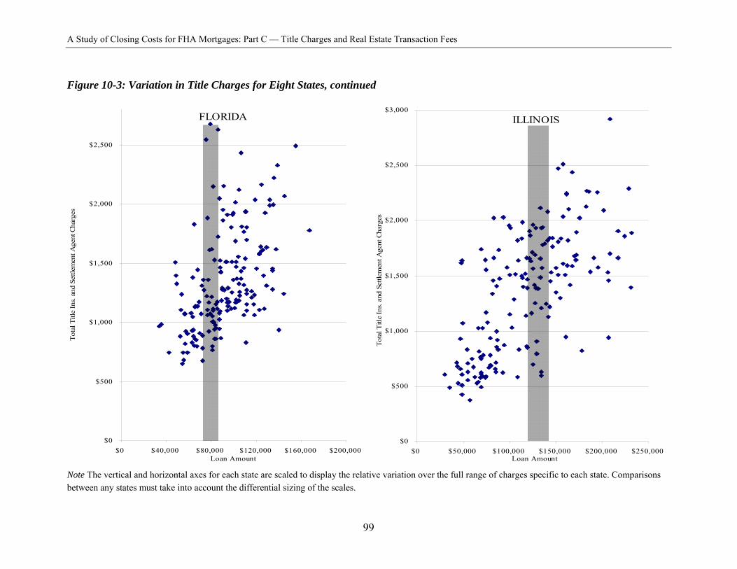
A Study of Closing Costs for FHA Mortgages: Part C — Title Charges and Real Estate Transaction Fees
Figure 10-3: Variation in Title Charges for Eight States, continued
$3,000
$2,500
FLORIDA
$2,500
$2,000
ILLINOIS
Tota
l Titl
e In
s. an
d Se
ttlem
ent A
gent
Cha
rges
Tota
l Titl
e In
s. an
d Se
ttlem
ent A
gent
Cha
rges
$2,000
$1,500
$1,500
$1,000 $1,000
$500 $500
$0 $0 $0 $40,000 $80,000 $120,000 $160,000 $200,000 $0 $50,000 $100,000 $150,000 $200,000 $250,000
Loan Amount Loan Amount
Note The vertical and horizontal axes for each state are scaled to display the relative variation over the full range of charges specific to each state. Comparisons between any states must take into account the differential sizing of the scales.
99
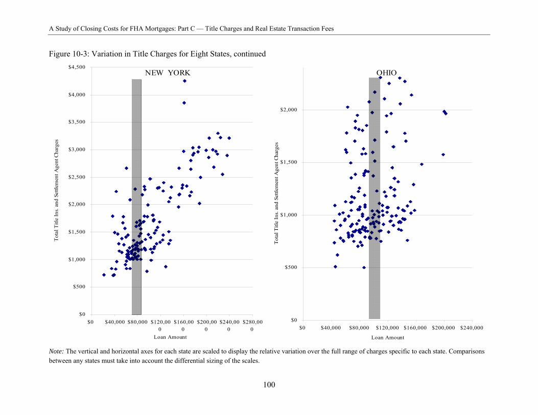
A Study of Closing Costs for FHA Mortgages: Part C — Title Charges and Real Estate Transaction Fees
Figure 10-3: Variation in Title Charges for Eight States, continued
$500
$500
$0 $0 $40,000 $80,000 $120,00 $160,00 $200,00 $240,00 $280,00 $0
0 0 0 0 0 $0 $40,000 $80,000 $120,000 $160,000 $200,000 $240,000
Loan Amount Loan Amount
OHIO
Note: The vertical and horizontal axes for each state are scaled to display the relative variation over the full range of charges specific to each state. Comparisons between any states must take into account the differential sizing of the scales.
$4,500
$4,000
NEW YORK
$2,000
$3,500
Tota
l Titl
e In
s. an
d Se
ttlem
ent A
gent
Cha
rges
$3,000
Tota
l Titl
e In
s. an
d Se
ttlem
ent A
gent
Cha
rges
$1,500
$2,500
$2,000
$1,000
$1,500
$1,000
100
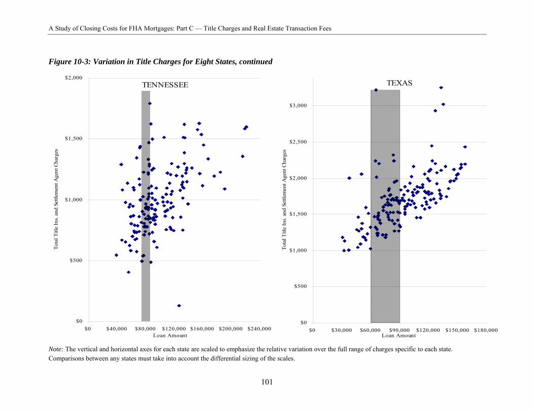
A Study of Closing Costs for FHA Mortgages: Part C — Title Charges and Real Estate Transaction Fees
Figure 10-3: Variation in Title Charges for Eight States, continued
$2,000 TENNESSEE
$3,000
$1,500 $2,500
TEXAS
Tota
l Titl
e In
s. an
d Se
ttlem
ent A
gent
Cha
rges
Tota
l Titl
e In
s. an
d Se
ttlem
ent A
gent
Cha
rges
$2,000
$1,000
$1,500
$1,000
$500
$500
$0 $0 $0 $40,000 $80,000 $120,000 $160,000 $200,000 $240,000 $0 $30,000 $60,000 $90,000 $120,000 $150,000 $180,000
Loan Amount Loan Amount
Note: The vertical and horizontal axes for each state are scaled to emphasize the relative variation over the full range of charges specific to each state. Comparisons between any states must take into account the differential sizing of the scales.
101
A Study of Closing Costs for FHA Mortgages: Part C — Title Charges and Real Estate Transaction Fees
These scatter diagrams show how much total title charges vary in individual states. In California, for loan amounts around $160,000, total title charges range from $1,500 to $2,900, with no evident clustering, though title charges on average rise with loan amount. In Connecticut, loans around $120,000 have title charges ranging from about $900 to over $2,400. Loans around $80,000 in Florida have total title charges from $800 to over $2,000. In Illinois, total title charges for a loan around $140,000 range from around $600 to $2,000. Loans of $80,000 in New York have total title charges from $1,000 to $2,200. Ohio has total title charges from $700 to over $2,000 for loans around $100,000. Loan amounts around $80,000 in Tennessee have title charges ranging from $500 to $1,500. Charges in Texas for loans from $60,000 to $90,000 range from $1,200 to over $2,200.
It is beyond the scope of this study to determine why title charges are so much higher in some states than in others. What this study does, for the first time, is offer some systematically collected data on just how much borrowers are charged for title services and establish that the differences by state are large. Even within each state, large variation unrelated to any competitive forces can be established.
Relation of Title Charges with Loan and Borrower Characteristics
The statistical analysis of title fees shows that title fees rise with loan amount, rise even faster with the amount of the borrower’s down payment, and also rise with neighborhood property values (the median home price in the borrower’s census tract). Title fees are unrelated to either borrower credit scores or whether borrowers have a credit score.
The underlying economics of title services suggests that the cost of assuring title and collecting and assembling the documents necessary to complete a loan closing should have little relation to the amount of the loan or the value of the property. While title insurance is indeed called insurance, the title industry itself emphasizes that the most important aspect of its service is the research done before putting a policy in place, not the insurance itself. For life insurance companies, roughly 95 percent of premiums are eventually paid out in claims to insured parties. For property and casualty insurance, roughly 80 percent of premiums are paid out in claims. For title insurance, less than 5 percent of premiums are paid out in claims. The title industry, when asked to explain these differences, identifies the efforts to identify and resolve title issues as central.
102
A Study of Closing Costs for FHA Mortgages: Part C — Title Charges and Real Estate Transaction Fees
Title fees are higher where area median income is higher, perhaps reflecting variation in local wage levels, a cost of doing business.
Title fees are higher in minority neighborhoods, other things equal. The race relationships in title charges are connected to the racial composition of the borrower’s census tract, but not to the race of the individual borrowers. Borrowers in a typical Latino borrower’s neighborhood pay an extra $106 for title services on average, and borrowers in an African-American neighborhood pay an additional $123, both compared to borrowers residing in neighborhoods with no minorities.
As with lender/broker fees, the education differential is large ($200) for completed-college versus no college, with borrowers in neighborhoods with lower levels of educational attainment paying more. See models 1 through 3 in table 16a in appendix I for the measurement details.
In some states, the services of a lawyer are required in connection with securing title, in others they are not. Among the total 7560 loans, 2,303 have payments to attorneys indicated in the 1100s on the HUD-1. The average attorney fees for nonsubsidized loans with any fees to attorneys are $400. Yet total title fees (including payments to attorneys) on the nonsubsidized loans where an attorney was compensated average $1,278, compared with. $1,179 on loans with no attorney. Thus, it appears that the requirement for an attorney in the loan raises fees only by about $100 despite the fees to the attorneys averaging $400. This difference suggests that attorney services mainly replace other title-related services. A regression of title fees on the usual set of borrower and loan characteristics produces a similar measure ($110) as the coefficient on a categorical variable indicating attorney services are present. (See model 4, table 16, appendix I.)
An additional finding here is that title fees are higher when lender/broker fees or realty fees are higher. These relations are present even when all other loan and borrower characteristics are taken into account, and they are measured with high precision. The amounts by which title fees are higher do not seem to be explainable by something simple, such as the cost to the title company of cutting a check to a lender or real estate agent. For example, title fees are about $20 higher for each consumer loan payoff made in connection with the new mortgage loan, a plausible cost for processing a check to a creditor (see the coefficient on the number of debt payoffs in model 2, table 16, appendix I). Looking at lender/broker fees, title fees are higher by 2.5 percent of the cash fees to lender/brokers and higher by 1.2 percent of the YSP. The strength and size of the effect differs from state to state. These coefficients are for the unsubsidized national sample.
103
A Study of Closing Costs for FHA Mortgages: Part C — Title Charges and Real Estate Transaction Fees
This elevation of fees does not reflect merely that all fees are higher on larger loans, because loan amount (as well as down payment and neighborhood property values) is already accounted for as part of the same measurement. Although title charges rise with both lender/broker charges and realty fees, there is no relationship between the fees paid to lender/brokers and to real estate agents. In other words, when either the lender or the real estate agent makes more on a deal, so does the title company, but the fees of lender/brokers and real estate agents have no similar relation to each other. Title fees rise with lender/broker and realty fees among the nonsubsidized loans.
A fee elevation of 2.5 percent may seem small, but it is not. For example, lender/broker fees on nonsubsidized loans average about $3,100 per loan among these FHA loans. The variation is large, and the 25th and 75th percentiles are roughly $1,950 and $4,350, a difference of $2,400. If these fees are split into half cash and half YSP, the title company makes an additional $100 on the 75th percentile loan versus the 25th percentile loan. This extra amount is in addition to the fees related strictly to loan amount, down payment, and neighborhood property values.
The relationship between title fees and the fees of lender/brokers is also present in the Woodward (2003) data. In her data, for a nationwide set of 2,650 brokered loans, funded from 1996 to 2001 by a single wholesale lender, title fees (reckoned in the same way as for these FHA loans, as all fees paid for services related to title in the 1100s of the HUD-1) averaged $1,175 on loans averaging $130,000 (standard deviation: $75,000). Using a specification as close as possible to the one used here for the FHA loans, including categorical (dummy) variables for all states (except Hawaii, for which there were no loans in the set), title charges were higher by 5.3 percent (standard error = 0.7 percent) of the cash paid to the lender/broker. In that study, no data were collected on fees to real estate agents.
Reflections on the Findings
The standard controversy on title insurance (whether referral fees raise or lower closing costs overall) is only partially informed by the findings here. The differences by state are so large, so systematic, and so different that variation in the success of tacit collusion (often blessed by state regulation) at the state level is a leading candidate for explaining them. The finding that title fees are higher when either lender/broker or realty fees are higher further undermines the hypothesis that competition among other suppliers of settlement services competes away the monopoly element of pricing for title services. The data cannot tell us why this is so: perhaps no referral
104
A Study of Closing Costs for FHA Mortgages: Part C — Title Charges and Real Estate Transaction Fees
fees are paid by title agents to real estate agents or to lender/brokers, or perhaps referral fees are paid but have no impact on the price of the bundle of services.
Title services are not governed by a simple, fixed-price monopoly. This market has substantial impediments to competition and little price transparency. The most systematic sources of variation other than state—notably loan amount, down payment amount, neighborhood racial composition, and education—appear to be simple price discrimination. These loan and borrower differences are not related (or in the case of loan amount, only weakly related) to the cost of providing title services, but they are clearly related to how much borrowers are charged. This price discrimination would not be possible if the market were transparent and competitive.
What neither traditional view of kickbacks or referral fees seems to contemplate is the possibility that title fees are higher when lender/broker or realty fees are higher, and the importance of the title agent’s position in the fee-setting sequence: charges for title services are determined only after the realty and lender/broker fees are known. This finding uncovers a different dynamic among settlement service providers. If the real estate agent or lender introduces a high-paying customer to the title agent, there is yet another reason to seek a kickback: the referrer knows that the title service agency is going to earn a premium on this customer and expects to be rewarded with some part of the gain. The traditional price theory of White and Owen presumes a well-informed competitive market where prices reach competitive equilibrium unless regulation gets in the way. It does not conceive of the possibility of situations such as the “$1,000 cash-back” deals on autos described in chapter 2 in which the sales people know that $1,000 is on the table but the customers do not. Or of customers who are confused about what price should be and vulnerable to noncompetitive variations in price at all levels.
It is widely believed that homebuyers and sellers do not shop for title services. In areas where traditionally the seller has paid for the lender’s title insurance, selecting a title agent is often left to the seller’s real estate agent. Either seller or buyer mainly takes the recommendation of a real estate agent or a lender for title services. Homebuyers also do not shop for services other than insurance provided by title companies. It is very rare to see payments to more than a single title company on a HUD-1. Indeed, the marketing efforts of local title service agencies are targeted at other settlement service providers, not at home sellers or buyers.
Homebuyers have good reasons to not shop for title services. First, they might presume that the market is competitive and that all the prices are the same, and that there is no payoff to shopping. Or they might assume that the market is regulated or be told by lenders, real estate agents, or
105
1
A Study of Closing Costs for FHA Mortgages: Part C — Title Charges and Real Estate Transaction Fees
even title agents that the market is regulated, that prices are fixed, and there is no point in shopping (the author has heard many personal accounts of being told this and also heard it for herself). Or homebuyers might presume that it is in the real estate agent or lender’s interest to guide them to the lowest cost provider to leave more money in the transaction for their own fees. All these reasons for not searching for the lowest price make economic sense. Add to this most buyers’ ignorance of the institutions of the real estate market (that the entire market is a negotiated market, that there are no truly fixed prices), plus their anxiety to get their deals closed, and they become highly inelastic demanders, constrained mainly by how much cash they have available given the house they have chosen, and vulnerable to price discrimination.
What policy change could bring more competition and lower prices to the market for title services? The findings on title fees suggest that improvements are possible, but it is the findings on lender/broker fees that offer guidance on how to reach them. The borrowers who got the best deals were those who got the simplest deals, the borrowers who took out “no-cost” loans. Two principles appear to operate in favor of the no-cost borrowers: simplified price shopping (no-cost borrowers can shop on rate alone because there are no up-front cash charges) and the commitment from the lender that the rate is set and no cash charges will be added between commitment and closing.
One way to simplify the closing transaction for borrowers and to introduce more forceful competition for title services is to allow lenders to arrange for title services as part of loan origination services, and to price the title services without pricing the individual items separately. The original price theory of Owen and White is not flawed, but it is incomplete. Competition works best when the prices are quoted clearly and simply.
In some places, notably British Columbia in Canada, the provincial government has efficiently created the necessary database for assuring clear title. Access to it is almost free. For $24 (Canadian) plus tax, British Columbia will deliver by email, in one day, a real estate title search using a parcel identifier.2 Title insurance is not part of property transactions in British Columbia. Appendix IV discusses the writings and research on title services.
106
A Study of Closing Costs for FHA Mortgages: Part C — Title Charges and Real Estate Transaction Fees
Chapter XI: Real Estate Transaction Fees
All the loans studied here are for the purchase of a home. Real estate agents were compensated in 81 percent of these purchases, while the other 19 percent were presumed sold by the owners. This 19 percent “FSBO” (for-sale-by-owner) or “fizbo” rate compares with a rate of 13 percent on all home transactions nationwide (reported by the National Association of Real Estate Agents) for the year 2000. A probability analysis of transactions studied here (model 1 of table 18 of appendix I) indicates that less-valuable houses are more likely to be sold by their owners without the assistance of a real estate agent. This is consistent with an FHA fizbo rate higher than the national average rate, because FHA limits the size of the loans it insures to target the program to less-affluent homebuyers.
The probit analysis also shows that houses are more likely to be sold without a real estate agent in areas where median metropolitan area income is low and when the individual buyer or borrower does not belong to a minority group (either African American or Latino). Real estate agents are more likely to be involved in the transaction when the buyer’s down payment is small and when the house is in a non-minority neighborhood.
Real estate agent fees are not uniform at six percent of house value. Instead, realty fees are well characterized as $970 plus 4.5 percent of the house value, with substantial variation around this average, shown in model 1 of table 17 of appendix I. Figure 11-1 below shows the distribution of real estate agent fees as a percent of property value.
107
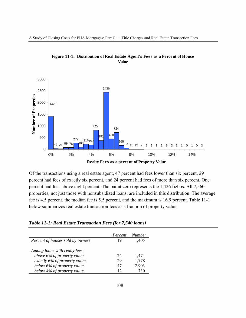
A Study of Closing Costs for FHA Mortgages: Part C — Title Charges and Real Estate Transaction Fees
Figure 11-1: Dis tribution of Re al Estate Age nt’s Fe e s as a Pe rce nt of House Value
43 26 89 76 57 9 6 3 3 1 3 3 1 1 0 1 0 3 0
272 103
216197
827
391
2436
450
724
165 16 12
500
1000
1500
2000
2500
3000
Num
ber
of P
rope
rtie
s
1426
0% 2% 4% 6% 8% 10% 12% 14%
Realty Fees as a percent of Property Value
Of the transactions using a real estate agent, 47 percent had fees lower than six percent, 29 percent had fees of exactly six percent, and 24 percent had fees of more than six percent. One percent had fees above eight percent. The bar at zero represents the 1,426 fizbos. All 7,560 properties, not just those with nonsubsidized loans, are included in this distribution. The average fee is 4.5 percent, the median fee is 5.5 percent, and the maximum is 16.9 percent. Table 11-1 below summarizes real estate transaction fees as a fraction of property value:
Table 11-1: Real Estate Transaction Fees (for 7,540 loans)
Percent Number Percent of houses sold by owners 19 1,405
Among loans with realty fees: above 6% of property value 24 1,474 exactly 6% of property value 29 1,778 below 6% of property value 47 2,903 below 4% of property value 12 730
108
A Study of Closing Costs for FHA Mortgages: Part C — Title Charges and Real Estate Transaction Fees
Real estate agents’ fees are related to more than just the value of the house. One can think of the value of the house as the sum of the loan amount plus the borrower’s down payment. Real estate agent’s fees rise faster with down payment than with loan amount. Another way of expressing this result is that for two houses of the same value, the real estate agent’s fees are lower when the buyer has a smaller down payment. Real estate agents’ fees rise with the fraction of adults who have a college education in a census tract. Real estate fees are $55 lower in typical Latino neighborhoods. The average Latino proportion of the neighborhoods of Latino borrowers is 27 percent (as compared with six percent for white borrowers). To explore this phenomenon, the analysis was repeated limiting the measurement to white borrowers only. White borrowers living in Latino neighborhoods enjoy a similar reduction in realty fees. Limiting the analysis to only African American borrowers reveals that African Americans living in Latino neighborhoods receive no reduction in realty fees.
The fees of real estate agents are not related to race or income of individual borrowers, or to neighborhood racial composition other than Latino. Real estate agent’s fees are positively related to the fees for title services on loans. This relationship is discussed in the section on title fees. Measurements for these results are in model 2 of table 17 in appendix I.
109
A Study of Closing Costs for FHA Mortgages: Appendixes
Appendix I: Econometric Measurements
I-1
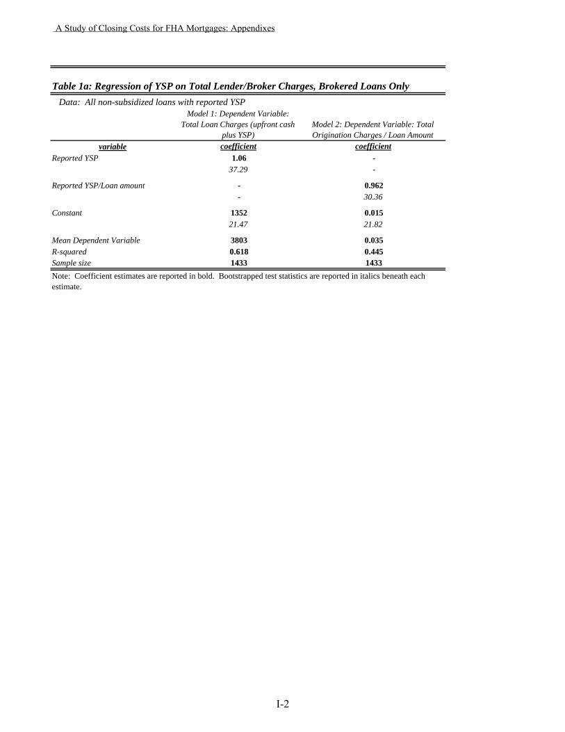
Table 1a: Regression of YSP on Total Lender/Broker Charges, Brokered Loans Only Data: All non-subsidized loans with reported YSP
Model 1: Dependent Variable: Total Loan Charges (upfront cash
plus YSP)Model 2: Dependent Variable: Total Origination Charges / Loan Amount
variable coefficient coefficientReported YSP 1.06 -
37.29 -
Reported YSP/Loan amount - 0.962- 30.36
Constant 1352 0.01521.47 21.82
Mean Dependent Variable 3803 0.035R-squared 0.618 0.445Sample size 1433 1433Note: Coefficient estimates are reported in bold. Bootstrapped test statistics are reported in italics beneath each estimate.
A Study of Closing Costs for FHA Mortgages: Appendixes
I-2
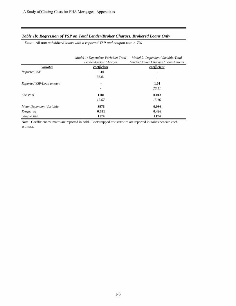
Table 1b: Regression of YSP on Total Lender/Broker Charges, Brokered Loans Only Data: All non-subsidized loans with a reported YSP and coupon rate > 7%
Model 1: Dependent Variable: Total Lender/Broker Charges
Model 2: Dependent Variable:Total Lender/Broker Charges / Loan Amount
variable coefficient coefficientReported YSP 1.10 -
36.01 -
Reported YSP/Loan amount - 1.01- 28.11
Constant 1181 0.01315.67 15.16
Mean Dependent Variable 3976 0.036R-squared 0.631 0.426Sample size 1174 1174
Note: Coefficient estimates are reported in bold. Bootstrapped test statistics are reported in italics beneath each estimate.
A Study of Closing Costs for FHA Mortgages: Appendixes
I-3
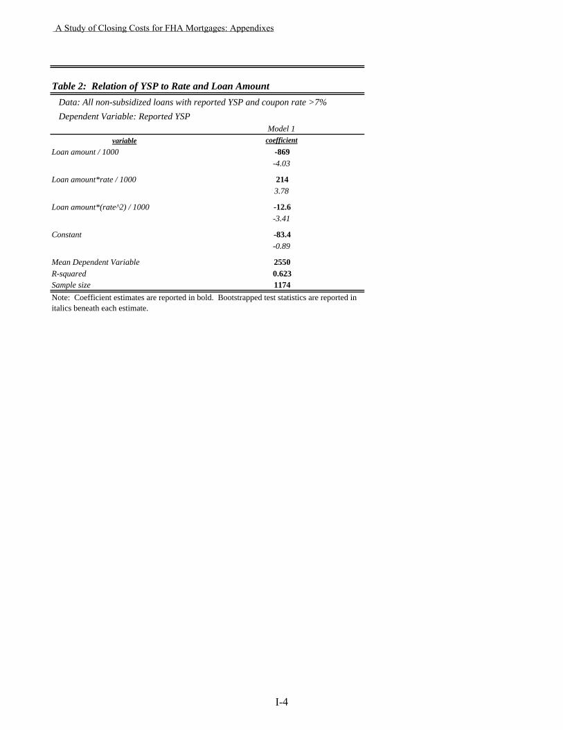
Table 2: Relation of YSP to Rate and Loan Amount Data: All non-subsidized loans with reported YSP and coupon rate >7% Dependent Variable: Reported YSP
Model 1variable coefficient
Loan amount / 1000 -869-4.03
Loan amount*rate / 1000 2143.78
Loan amount*(rate^2) / 1000 -12.6-3.41
Constant -83.4-0.89
Mean Dependent Variable 2550R-squared 0.623Sample size 1174Note: Coefficient estimates are reported in bold. Bootstrapped test statistics are reported in italics beneath each estimate.
A Study of Closing Costs for FHA Mortgages: Appendixes
I-4
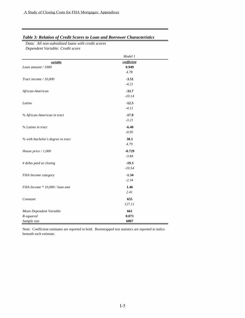
Table 3: Relation of Credit Scores to Loan and Borrower Characteristics Data: All non-subsidized loans with credit scores Dependent Variable: Credit score
Model 1variable coefficient
Loan amount / 1000 0.9494.78
Tract income / 10,000 -3.51-4.21
African-American -33.7-10.14
Latino -12.5-4.11
% African-American in tract -17.9-3.21
% Latino in tract -6.40-0.95
% with bachelor's degree in tract 38.14.79
House price / 1,000 -0.729-3.84
# debts paid at closing -19.3-10.54
FHA Income category -1.34-2.34
FHA Income * 10,000 / loan amt 1.462.41
Constant 655127.11
Mean Dependent Variable 661R-squared 0.071Sample size 6007
Note: Coefficient estimates are reported in bold. Bootstrapped test statistics are reported in italics beneath each estimate.
A Study of Closing Costs for FHA Mortgages: Appendixes
I-5
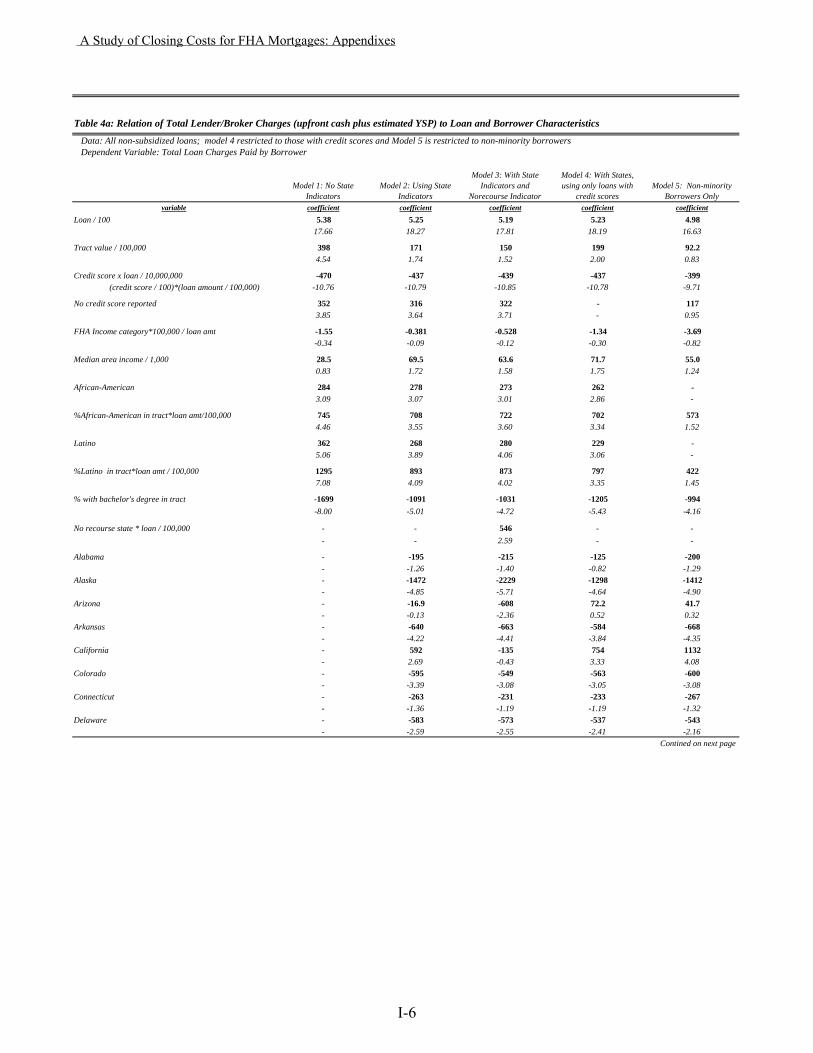
Data: All non-subsidized loans; model 4 restricted to those with credit scores and Model 5 is restricted to non-minority borrowers Dependent Variable: Total Loan Charges Paid by Borrower
Model 1: No State Indicators
Model 2: Using State Indicators
Model 3: With State Indicators and
Norecourse Indicator
Model 4: With States, using only loans with
credit scoresModel 5: Non-minority
Borrowers Onlyvariable coefficient coefficient coefficient coefficient coefficient
Loan / 100 5.38 5.25 5.19 5.23 4.9817.66 18.27 17.81 18.19 16.63
Tract value / 100,000 398 171 150 199 92.24.54 1.74 1.52 2.00 0.83
Credit score x loan / 10,000,000 -470 -437 -439 -437 -399 (credit score / 100)*(loan amount / 100,000) -10.76 -10.79 -10.85 -10.78 -9.71
No credit score reported 352 316 322 - 1173.85 3.64 3.71 - 0.95
FHA Income category*100,000 / loan amt -1.55 -0.381 -0.528 -1.34 -3.69-0.34 -0.09 -0.12 -0.30 -0.82
Median area income / 1,000 28.5 69.5 63.6 71.7 55.00.83 1.72 1.58 1.75 1.24
African-American 284 278 273 262 -3.09 3.07 3.01 2.86 -
%African-American in tract*loan amt/100,000 745 708 722 702 5734.46 3.55 3.60 3.34 1.52
Latino 362 268 280 229 -5.06 3.89 4.06 3.06 -
%Latino in tract*loan amt / 100,000 1295 893 873 797 4227.08 4.09 4.02 3.35 1.45
% with bachelor's degree in tract -1699 -1091 -1031 -1205 -994-8.00 -5.01 -4.72 -5.43 -4.16
No recourse state * loan / 100,000 - - 546 - -- - 2.59 - -
Alabama - -195 -215 -125 -200- -1.26 -1.40 -0.82 -1.29
Alaska - -1472 -2229 -1298 -1412- -4.85 -5.71 -4.64 -4.90
Arizona - -16.9 -608 72.2 41.7- -0.13 -2.36 0.52 0.32
Arkansas - -640 -663 -584 -668- -4.22 -4.41 -3.84 -4.35
California - 592 -135 754 1132- 2.69 -0.43 3.33 4.08
Colorado - -595 -549 -563 -600- -3.39 -3.08 -3.05 -3.08
Connecticut - -263 -231 -233 -267- -1.36 -1.19 -1.19 -1.32
Delaware - -583 -573 -537 -543- -2.59 -2.55 -2.41 -2.16
Contined on next page
Table 4a: Relation of Total Lender/Broker Charges (upfront cash plus estimated YSP) to Loan and Borrower Characteristics
A Study of Closing Costs for FHA Mortgages: Appendixes
I-6
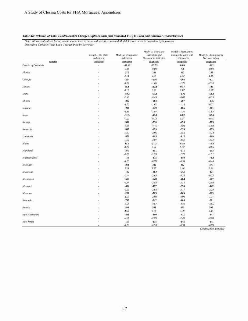
Data: All non-subsidized loans; model 4 restricted to those with credit scores and Model 5 is restricted to non-minority borrowers Dependent Variable: Total Loan Charges Paid by Borrower
Model 1: No State Indicators
Model 2: Using State Indicators
Model 3: With State Indicators and
Norecourse Indicator
Model 4: With States, using only loans with
credit scoresModel 5: Non-minority
Borrowers Onlyvariable coefficient coefficient coefficient coefficient coefficient
Table 4a: Relation of Total Lender/Broker Charges (upfront cash plus estimated YSP) to Loan and Borrower Characteristics
District of Columbia - -49.13 -25.72 0.60 -912- -0.16 -0.08 NA -0.89
Florida - 272 261 353 168- 2.14 2.05 2.82 1.18
Georgia - -264 -256 -265 -371- -1.72 -1.66 -1.72 -2.30
Hawaii - 60.1 122.1 95.7 146- 0.11 0.22 0.17 0.27
Idaho - -59.2 -67.1 -1.72 -58.8- -0.43 -0.49 -0.01 -0.39
Illinois - -282 -263 -207 -135- -1.72 -1.61 -1.19 -0.71
Indiana - -236 -249 -166 -261- -1.86 -1.97 -1.30 -1.85
Iowa - -31.5 -48.8 6.82 -67.6- -0.21 -0.33 0.04 -0.45
Kansas - -516 -530 -459 -573- -4.30 -4.45 -3.84 -5.03
Kentucky - -617 -629 -555 -673- -3.87 -3.95 -3.52 -4.24
Louisiana - -679 -695 -612 -689- -3.91 -4.01 -3.52 -3.72
Maine - 45.6 37.3 81.8 -10.6- 0.29 0.24 0.52 -0.06
Maryland - -375 -351 -311 -293- -2.08 -1.95 -1.71 -1.51
Massachusetts - -178 -135 -159 -72.9- -1.03 -0.78 -0.94 -0.44
Michigan - 393 392 422 375- 3.28 3.27 3.46 2.91
Minnesota - -122 -802 -63.7 -121- -0.74 -2.63 -0.39 -0.72
Mississippi - -508 -528 -464 -507- -3.44 -3.58 -3.11 -2.98
Missouri - -404 -417 -356 -442- -3.55 -3.68 -3.17 -3.29
Montana - -222 -765 -169 -303- -1.25 -2.90 -0.94 -1.71
Nebraska - -737 -747 -684 -761- -4.59 -4.67 -4.30 -4.85
Nevada - 494 509 473 596- 3.60 3.70 3.39 3.45
New Hampshire - -496 -460 -411 -447- -2.96 -2.73 -2.43 -2.68
New Jersey - -159 -135 -145 -141- -1.06 -0.90 -0.94 -0.79
Continued on next page
A Study of Closing Costs for FHA Mortgages: Appendixes
I-7

Data: All non-subsidized loans; model 4 restricted to those with credit scores and Model 5 is restricted to non-minority borrowers Dependent Variable: Total Loan Charges Paid by Borrower
Model 1: No State Indicators
Model 2: Using State Indicators
Model 3: With State Indicators and
Norecourse Indicator
Model 4: With States, using only loans with
credit scoresModel 5: Non-minority
Borrowers Onlyvariable coefficient coefficient coefficient coefficient coefficient
Table 4a: Relation of Total Lender/Broker Charges (upfront cash plus estimated YSP) to Loan and Borrower Characteristics
New Mexico - -128 -130 -35.8 118- -0.60 -0.61 -0.17 0.55
New York - 145 149 221 -82.2- 0.98 1.00 1.50 -0.56
North Carolina - -278 -275 -169 -172- -1.52 -1.51 -0.91 -0.78
North Dakota - -687 -1169 -635 -772- -2.73 -3.87 -2.54 -2.91
Ohio - 177 173 233 125- 1.34 1.32 1.76 0.87
Oklahoma - -373 -400 -330 -425- -2.09 -2.27 -1.73 -2.26
Oregon - -30.4 -668.0 34.5 -189- -0.13 -2.07 0.16 -0.79
Pennsylvania - -293 -308 -242 -320- -2.47 -2.61 -2.00 -2.41
Rhode Island - -266 -249 -263 -344- -1.72 -1.60 -1.67 -2.04
South Carolina - -609 -619 -584 -606- -2.95 -3.01 -2.77 -2.56
South Dakota - -415 -433 -364 -497- -2.56 -2.70 -2.25 -3.09
Tennessee - -935 -941 -878 -887- -4.45 -4.48 -4.08 -4.15
Texas - -120 -130 -55.8 -174- -0.89 -0.98 -0.40 -1.10
Utah - 346 367 213 225- 1.16 1.22 0.70 0.60
Vermont - -219 -221 -141 -276- -1.23 -1.24 -0.80 -1.65
Virginia - -555 -533 -494 -532- -3.30 -3.16 -2.87 -2.77
Washington - 467 -247 482 458- 2.57 -0.89 2.63 2.09
West Virginia - -111 -123 -56.5 -159- -0.87 -0.97 -0.45 -1.21
Wyoming - -1176 -1180 -1092 -1173- -3.71 -3.72 -3.48 -3.70
Constant 143.1 265 370 236 4850.93 1.40 1.93 1.22 2.47
Mean Dependent Variable 3100 3100 3100 3082 2915R-squared 0.391 0.434 0.435 0.430 0.397Sample size 6366 6366 6366 6007 5065
Note: Coefficient estimates are reported in bold. Bootstrapped test statistics are reported in italics beneath each estimate.
A Study of Closing Costs for FHA Mortgages: Appendixes
I-8
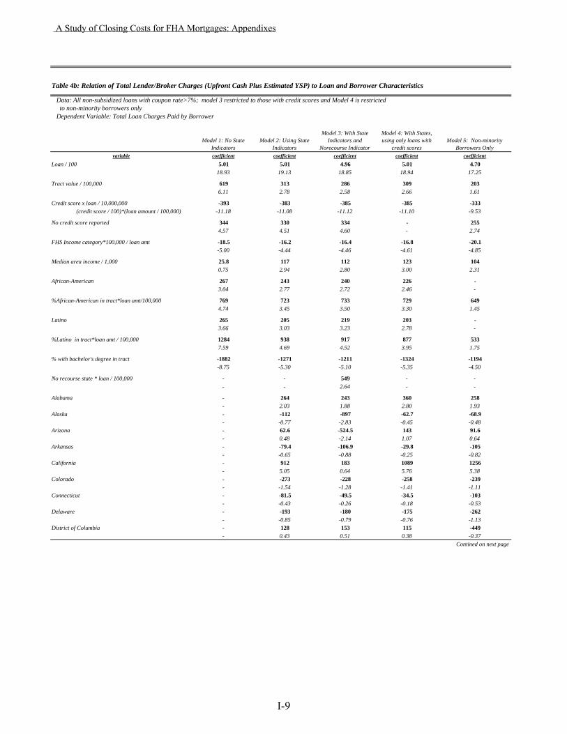
Data: All non-subsidized loans with coupon rate>7%; model 3 restricted to those with credit scores and Model 4 is restricted to non-minority borrowers only Dependent Variable: Total Loan Charges Paid by Borrower
Model 1: No State Indicators
Model 2: Using State Indicators
Model 3: With State Indicators and
Norecourse Indicator
Model 4: With States, using only loans with
credit scoresModel 5: Non-minority
Borrowers Onlyvariable coefficient coefficient coefficient coefficient coefficient
Loan / 100 5.01 5.01 4.96 5.01 4.7018.93 19.13 18.85 18.94 17.25
Tract value / 100,000 619 313 286 309 2036.11 2.78 2.58 2.66 1.61
Credit score x loan / 10,000,000 -393 -383 -385 -385 -333 (credit score / 100)*(loan amount / 100,000) -11.18 -11.08 -11.12 -11.10 -9.53
No credit score reported 344 330 334 - 2554.57 4.51 4.60 - 2.74
FHS Income category*100,000 / loan amt -18.5 -16.2 -16.4 -16.8 -20.1-5.00 -4.44 -4.46 -4.61 -4.85
Median area income / 1,000 25.8 117 112 123 1040.75 2.94 2.80 3.00 2.31
African-American 267 243 240 226 -3.04 2.77 2.72 2.46 -
%African-American in tract*loan amt/100,000 769 723 733 729 6494.74 3.45 3.50 3.30 1.45
Latino 265 205 219 203 -3.66 3.03 3.23 2.78 -
%Latino in tract*loan amt / 100,000 1284 938 917 877 5337.59 4.69 4.52 3.95 1.75
% with bachelor's degree in tract -1882 -1271 -1211 -1324 -1194-8.75 -5.30 -5.10 -5.35 -4.50
No recourse state * loan / 100,000 - - 549 - -- - 2.64 - -
Alabama - 264 243 360 258- 2.03 1.88 2.80 1.93
Alaska - -112 -897 -62.7 -68.9- -0.77 -2.83 -0.45 -0.48
Arizona - 62.6 -524.5 143 91.6- 0.48 -2.14 1.07 0.64
Arkansas - -79.4 -106.9 -29.8 -105- -0.65 -0.88 -0.25 -0.82
California - 912 183 1089 1256- 5.05 0.64 5.76 5.38
Colorado - -273 -228 -258 -239- -1.54 -1.28 -1.41 -1.11
Connecticut - -81.5 -49.5 -34.5 -103- -0.43 -0.26 -0.18 -0.53
Delaware - -193 -180 -175 -262- -0.85 -0.79 -0.76 -1.13
District of Columbia - 128 153 115 -449- 0.43 0.51 0.38 -0.37
Contined on next page
Table 4b: Relation of Total Lender/Broker Charges (Upfront Cash Plus Estimated YSP) to Loan and Borrower Characteristics
A Study of Closing Costs for FHA Mortgages: Appendixes
I-9
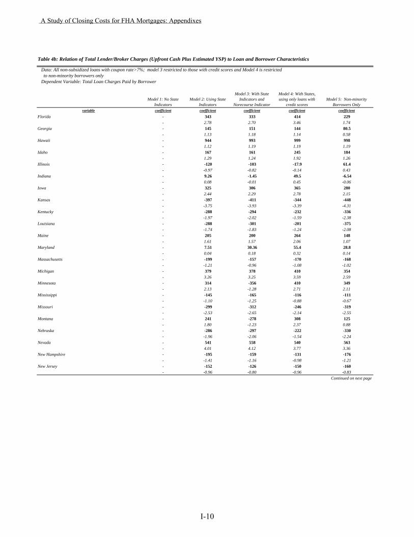
Data: All non-subsidized loans with coupon rate>7%; model 3 restricted to those with credit scores and Model 4 is restricted to non-minority borrowers only Dependent Variable: Total Loan Charges Paid by Borrower
Model 1: No State Indicators
Model 2: Using State Indicators
Model 3: With State Indicators and
Norecourse Indicator
Model 4: With States, using only loans with
credit scoresModel 5: Non-minority
Borrowers Onlyvariable coefficient coefficient coefficient coefficient coefficient
Table 4b: Relation of Total Lender/Broker Charges (Upfront Cash Plus Estimated YSP) to Loan and Borrower Characteristics
Florida - 343 333 414 229- 2.78 2.70 3.46 1.74
Georgia - 145 151 144 80.5- 1.13 1.18 1.14 0.58
Hawaii - 944 993 999 998- 1.12 1.19 1.19 1.19
Idaho - 167 161 245 184- 1.29 1.24 1.92 1.26
Illinois - -120 -103 -17.9 61.4- -0.97 -0.82 -0.14 0.43
Indiana - 9.26 -1.45 49.5 -6.54- 0.08 -0.01 0.45 -0.06
Iowa - 325 306 365 280- 2.44 2.29 2.78 2.15
Kansas - -397 -411 -344 -448- -3.75 -3.93 -3.39 -4.31
Kentucky - -288 -294 -232 -336- -1.97 -2.02 -1.59 -2.38
Louisiana - -288 -301 -201 -375- -1.74 -1.83 -1.24 -2.08
Maine - 205 200 264 148- 1.61 1.57 2.06 1.07
Maryland - 7.51 30.36 55.4 28.8- 0.04 0.18 0.32 0.14
Massachusetts - -199 -157 -170 -168- -1.21 -0.96 -1.08 -1.02
Michigan - 379 378 410 354- 3.26 3.25 3.59 2.59
Minnesota - 314 -356 410 349- 2.13 -1.28 2.71 2.11
Mississippi - -145 -165 -116 -111- -1.10 -1.25 -0.88 -0.67
Missouri - -299 -312 -246 -319- -2.53 -2.65 -2.14 -2.55
Montana - 241 -278 308 125- 1.80 -1.23 2.37 0.88
Nebraska - -286 -297 -222 -330- -1.96 -2.06 -1.54 -2.24
Nevada - 541 558 540 563- 4.01 4.12 3.77 3.36
New Hampshire - -195 -159 -131 -176- -1.41 -1.16 -0.98 -1.21
New Jersey - -152 -126 -150 -160- -0.96 -0.80 -0.96 -0.83
Continued on next page
A Study of Closing Costs for FHA Mortgages: Appendixes
I-10
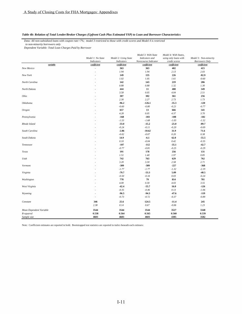
Data: All non-subsidized loans with coupon rate>7%; model 3 restricted to those with credit scores and Model 4 is restricted to non-minority borrowers only Dependent Variable: Total Loan Charges Paid by Borrower
Model 1: No State Indicators
Model 2: Using State Indicators
Model 3: With State Indicators and
Norecourse Indicator
Model 4: With States, using only loans with
credit scoresModel 5: Non-minority
Borrowers Onlyvariable coefficient coefficient coefficient coefficient coefficient
Table 4b: Relation of Total Lender/Broker Charges (Upfront Cash Plus Estimated YSP) to Loan and Borrower Characteristics
New Mexico - 363 363 402 415- 1.94 1.94 2.13 2.03
New York - 149 155 226 -82.9- 1.02 1.05 1.61 -0.60
North Carolina - 142 143 219 286- 0.88 0.88 1.32 1.30
North Dakota - 444 11 488 349- 3.58 0.05 4.04 2.51
Ohio - 307 302 361 256- 2.30 2.27 2.73 1.73
Oklahoma - -96.2 -126.1 -35.3 -120- -0.60 -0.80 -0.21 -0.77
Oregon - 657 13 666 541- 4.28 0.05 4.37 3.70
Pennsylvania - -168 -183 -108 -182- -1.53 -1.68 -1.03 -1.52
Rhode Island - -33.0 -15.2 -25.0 -89.7- -0.24 -0.11 -0.20 -0.69
South Carolina - -2.86 -10.62 31.9 71.6- -0.02 -0.07 0.20 0.38
South Dakota - 14.9 -6.1 62.0 -55.5- 0.10 -0.04 0.42 -0.35
Tennessee - -107 -112 -35.1 -42.7- -0.77 -0.81 -0.25 -0.29
Texas - 191 178 256 131- 1.51 1.40 1.97 0.85
Utah - 742 763 629 762- 3.20 3.30 2.58 2.71
Vermont - -309 -309 -227 -368- -1.77 -1.77 -1.32 -2.19
Virginia - -79.7 -53.3 5.09 -48.5- -0.50 -0.34 0.03 -0.24
Washington - 778 79 814 781- 4.00 0.30 4.03 3.55
West Virginia - -42.4 -55.7 16.0 -126- -0.35 -0.46 0.13 -1.06
Wyoming - -96.5 -94.3 -47.6 -119- -0.73 -0.72 -0.37 -0.89
Constant 346 25.6 124.5 -11.4 2452.38 0.14 0.67 -0.06 1.23
Mean Dependent Variable 3544 3544 3544 3527 3348R-squared 0.538 0.564 0.565 0.560 0.539Sample size 4603 4603 4603 4305 3582
Note: Coefficient estimates are reported in bold. Bootstrapped test statistics are reported in italics beneath each estimate.
A Study of Closing Costs for FHA Mortgages: Appendixes
I-11
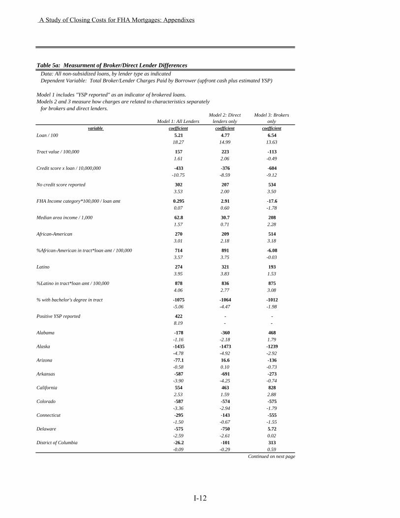
Table 5a: Measurment of Broker/Direct Lender Differences Data: All non-subsidized loans, by lender type as indicated Dependent Variable: Total Broker/Lender Charges Paid by Borrower (upfront cash plus estimated YSP)
Model 1 includes "YSP reported" as an indicator of brokered loans.Models 2 and 3 measure how charges are related to characteristics separately for brokers and direct lenders.
Model 1: All LendersModel 2: Direct
lenders onlyModel 3: Brokers
onlyvariable coefficient coefficient coefficient
Loan / 100 5.21 4.77 6.5418.27 14.99 13.63
Tract value / 100,000 157 223 -1131.61 2.06 -0.49
Credit score x loan / 10,000,000 -433 -376 -604-10.75 -8.59 -9.12
No credit score reported 302 207 5343.53 2.00 3.50
FHA Income category*100,000 / loan amt 0.295 2.91 -17.60.07 0.60 -1.78
Median area income / 1,000 62.8 30.7 2081.57 0.71 2.28
African-American 270 209 5143.01 2.18 3.18
%African-American in tract*loan amt / 100,000 714 891 -6.083.57 3.75 -0.03
Latino 274 321 1933.95 3.83 1.53
%Latino in tract*loan amt / 100,000 878 836 8754.06 2.77 3.08
% with bachelor's degree in tract -1075 -1064 -1012-5.06 -4.47 -1.98
Positive YSP reported 422 - -8.19 - -
Alabama -178 -360 468-1.16 -2.18 1.79
Alaska -1435 -1473 -1239-4.78 -4.92 -2.92
Arizona -77.1 16.6 -136-0.58 0.10 -0.73
Arkansas -587 -691 -273-3.90 -4.25 -0.74
California 554 463 8282.53 1.59 2.88
Colorado -587 -574 -575-3.36 -2.94 -1.79
Connecticut -295 -143 -555-1.50 -0.67 -1.55
Delaware -575 -750 5.72-2.59 -2.61 0.02
District of Columbia -26.2 -101 313-0.09 -0.29 0.59
Continued on next page
A Study of Closing Costs for FHA Mortgages: Appendixes
I-12
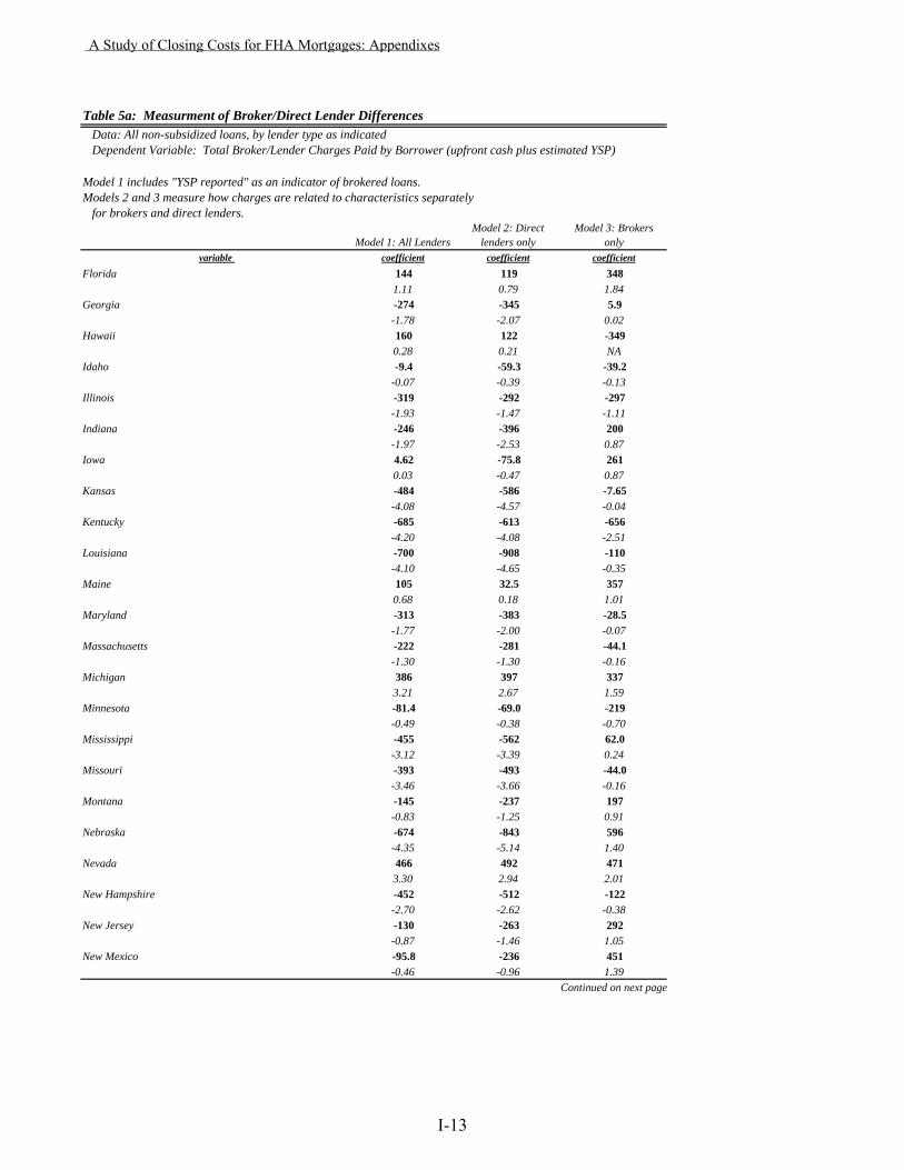
Table 5a: Measurment of Broker/Direct Lender Differences Data: All non-subsidized loans, by lender type as indicated Dependent Variable: Total Broker/Lender Charges Paid by Borrower (upfront cash plus estimated YSP)
Model 1 includes "YSP reported" as an indicator of brokered loans.Models 2 and 3 measure how charges are related to characteristics separately for brokers and direct lenders.
Model 1: All LendersModel 2: Direct
lenders onlyModel 3: Brokers
onlyvariable coefficient coefficient coefficient
Florida 144 119 3481.11 0.79 1.84
Georgia -274 -345 5.9-1.78 -2.07 0.02
Hawaii 160 122 -3490.28 0.21 NA
Idaho -9.4 -59.3 -39.2-0.07 -0.39 -0.13
Illinois -319 -292 -297-1.93 -1.47 -1.11
Indiana -246 -396 200-1.97 -2.53 0.87
Iowa 4.62 -75.8 2610.03 -0.47 0.87
Kansas -484 -586 -7.65-4.08 -4.57 -0.04
Kentucky -685 -613 -656-4.20 -4.08 -2.51
Louisiana -700 -908 -110-4.10 -4.65 -0.35
Maine 105 32.5 3570.68 0.18 1.01
Maryland -313 -383 -28.5-1.77 -2.00 -0.07
Massachusetts -222 -281 -44.1-1.30 -1.30 -0.16
Michigan 386 397 3373.21 2.67 1.59
Minnesota -81.4 -69.0 -219-0.49 -0.38 -0.70
Mississippi -455 -562 62.0-3.12 -3.39 0.24
Missouri -393 -493 -44.0-3.46 -3.66 -0.16
Montana -145 -237 197-0.83 -1.25 0.91
Nebraska -674 -843 596-4.35 -5.14 1.40
Nevada 466 492 4713.30 2.94 2.01
New Hampshire -452 -512 -122-2.70 -2.62 -0.38
New Jersey -130 -263 292-0.87 -1.46 1.05
New Mexico -95.8 -236 451-0.46 -0.96 1.39
Continued on next page
A Study of Closing Costs for FHA Mortgages: Appendixes
I-13
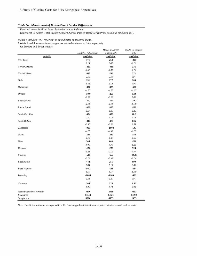
Table 5a: Measurment of Broker/Direct Lender Differences Data: All non-subsidized loans, by lender type as indicated Dependent Variable: Total Broker/Lender Charges Paid by Borrower (upfront cash plus estimated YSP)
Model 1 includes "YSP reported" as an indicator of brokered loans.Models 2 and 3 measure how charges are related to characteristics separately for brokers and direct lenders.
Model 1: All LendersModel 2: Direct
lenders onlyModel 3: Brokers
onlyvariable coefficient coefficient coefficient
New York 171 253 -3201.14 1.47 -1.01
North Carolina -260 -416 331-1.45 -2.18 0.78
North Dakota -632 -796 571-2.57 -2.89 NA
Ohio 191 177 2091.46 1.14 0.90
Oklahoma -337 -375 -586-1.87 -1.87 -1.67
Oregon -50.0 -260 520-0.22 -0.96 1.86
Pennsylvania -307 -390 -79.3-2.60 -2.68 -0.38
Rhode Island -300 -305 -220-1.94 -1.43 -1.11
South Carolina -554 -680 46.6-2.72 -3.09 0.16
South Dakota -344 -470 635-2.17 -2.80 1.53
Tennessee -905 -1004 -547-4.35 -4.42 -1.69
Texas -136 -232 156-1.02 -1.45 0.68
Utah 305 603 -2211.00 1.39 -0.65
Vermont -152 -278 924-0.88 -2.01 0.57
Virginia -510 -652 -14.86-3.06 -3.48 -0.04
Washington 444 255 8992.44 1.19 2.46
West Virginia -94.2 -111 -214-0.73 -0.74 -0.60
Wyoming -1084 -1160 -403-3.46 -3.67 NA
Constant 204 374 9.501.09 1.74 0.03
Mean Dependent Variable 3100 2939 3653R-squared 0.443 0.421 0.490Sample size 6366 4933 1433
Note: Coefficient estimates are reported in bold. Bootstrapped test statistics are reported in italics beneath each estimate.
A Study of Closing Costs for FHA Mortgages: Appendixes
I-14
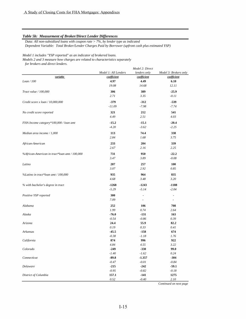
Table 5b: Measurment of Broker/Direct Lender Differences Data: All non-subsidized loans with coupon rate > 7%, by lender type as indicated Dependent Variable: Total Broker/Lender Charges Paid by Borrower (upfront cash plus estimated YSP)
Model 1 includes "YSP reported" as an indicator of brokered loans.Models 2 and 3 measure how charges are related to characteristics separately for brokers and direct lenders.
Model 1: All LendersModel 2: Direct
lenders only Model 3: Brokers onlyvariable coefficient coefficient coefficient
Loan / 100 4.97 4.49 6.1019.08 14.68 12.11
Tract value / 100,000 306 389 -25.92.71 3.35 -0.11
Credit score x loan / 10,000,000 -379 -312 -539-11.09 -7.98 -7.74
No credit score reported 321 212 5414.49 2.51 4.03
FHA Income category*100,000 / loan amt -15.2 -15.1 -20.4-4.20 -3.62 -2.25
Median area income / 1,000 113 74.4 3382.84 1.68 3.75
African-American 233 204 3392.67 2.16 2.25
%African-American in tract*loan amt / 100,000 731 950 -22.23.47 3.89 -0.08
Latino 207 257 1003.07 2.92 0.85
%Latino in tract*loan amt / 100,000 935 964 8354.68 3.48 3.20
% with bachelor's degree in tract -1268 -1243 -1188-5.29 -5.14 -2.04
Positive YSP reported 300 - -7.09 - -
Alabama 252 106 7081.99 0.74 2.64
Alaska -76.0 -131 163-0.54 -0.86 0.39
Arizona 24.4 55.9 82.20.19 0.33 0.41
Arkansas -45.5 -158 674-0.38 -1.18 1.76
California 874 996 9224.84 4.55 3.22
Colorado -249 -330 99.0-1.40 -1.62 0.24
Connecticut -89.8 -1.357 -304-0.47 -0.01 -0.84
Delaware -215 -242 -59.1-0.95 -0.82 -0.18
District of Columbia 157.1 -141 12750.52 -0.40 2.10
Continued on next page
A Study of Closing Costs for FHA Mortgages: Appendixes
I-15
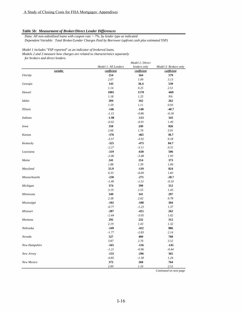
Table 5b: Measurment of Broker/Direct Lender Differences Data: All non-subsidized loans with coupon rate > 7%, by lender type as indicated Dependent Variable: Total Broker/Lender Charges Paid by Borrower (upfront cash plus estimated YSP)
Model 1 includes "YSP reported" as an indicator of brokered loans.Models 2 and 3 measure how charges are related to characteristics separately for brokers and direct lenders.
Model 1: All LendersModel 2: Direct
lenders only Model 3: Brokers onlyvariable coefficient coefficient coefficient
Florida 254 164 5792.07 1.09 3.13
Georgia 143 36.4 5391.14 0.25 2.51
Hawaii 1001 1170 -6691.18 1.25 NA
Idaho 204 162 2621.59 1.11 0.93
Illinois -146 -140 -40.7-1.15 -0.86 -0.18
Indiana -1.98 -113 343-0.02 -0.91 1.49
Iowa 350 249 8262.66 1.76 3.01
Kansas -376 -465 38.7-3.57 -3.92 0.18
Kentucky -325 -473 84.7-2.27 -3.11 0.31
Louisiana -319 -630 506-2.06 -3.48 1.93
Maine 241 214 3731.88 1.39 1.00
Maryland 55.9 -119 8240.33 -0.69 1.83
Massachusetts -230 -271 -28.7-1.40 -1.51 -0.10
Michigan 374 390 3123.19 2.55 1.43
Minnesota 349 341 2972.38 2.02 0.78
Mississippi -102 -188 304-0.77 -1.23 1.37
Missouri -287 -415 262-2.44 -3.05 1.02
Montana 292 232 3122.19 1.43 1.32
Nebraska -249 -422 886-1.77 -2.83 2.14
Nevada 527 460 7683.87 2.76 3.52
New Hampshire -165 -156 -145-1.21 -0.96 -0.44
New Jersey -133 -296 365-0.85 -1.58 1.24
New Mexico 372 268 7642.00 1.16 2.51
Continued on next page
A Study of Closing Costs for FHA Mortgages: Appendixes
I-16
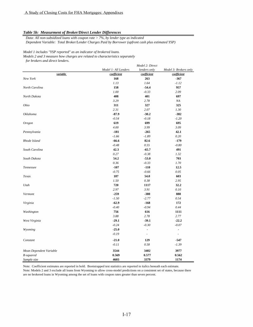
Table 5b: Measurment of Broker/Direct Lender Differences Data: All non-subsidized loans with coupon rate > 7%, by lender type as indicated Dependent Variable: Total Broker/Lender Charges Paid by Borrower (upfront cash plus estimated YSP)
Model 1 includes "YSP reported" as an indicator of brokered loans.Models 2 and 3 measure how charges are related to characteristics separately for brokers and direct lenders.
Model 1: All LendersModel 2: Direct
lenders only Model 3: Brokers onlyvariable coefficient coefficient coefficient
New York 168 263 -3671.13 1.64 -1.12
North Carolina 158 -54.4 9571.00 -0.33 2.09
North Dakota 408 401 6973.29 2.78 NA
Ohio 311 327 3252.31 2.07 1.30
Oklahoma -87.9 -30.2 -382-0.54 -0.18 -1.20
Oregon 619 699 6954.00 3.99 3.09
Pennsylvania -181 -265 42.1-1.66 -1.89 0.20
Rhode Island -66.6 82.6 -179-0.48 0.55 -0.80
South Carolina 42.3 -65.7 4910.27 -0.38 1.32
South Dakota 54.2 -53.0 7030.36 -0.33 1.70
Tennessee -107 -110 12.5-0.75 -0.66 0.05
Texas 187 54.0 6031.50 0.38 2.95
Utah 720 1117 32.22.97 3.91 0.10
Vermont -259 -380 888-1.50 -2.77 0.54
Virginia -62.9 -168 172-0.40 -0.94 0.44
Washington 756 616 11113.88 2.78 2.77
West Virginia -29.1 -39.1 -22.2-0.24 -0.30 -0.07
Wyoming -25.0 - --0.19 - -
Constant -21.0 129 -547-0.11 0.58 -1.39
Mean Dependent Variable 3544 3402 3977R-squared 0.569 0.577 0.562Sample size 4603 3379 1174
Note: Coefficient estimates are reported in bold. Bootstrapped test statistics are reported in italics beneath each estimate.Note: Models 2 and 3 exclude all loans from Wyoming to allow cross-model predictions on a consistent set of states, because there are no brokered loans in Wyoming among the set of loans with coupon rates greater than seven percent.
A Study of Closing Costs for FHA Mortgages: Appendixes
I-17
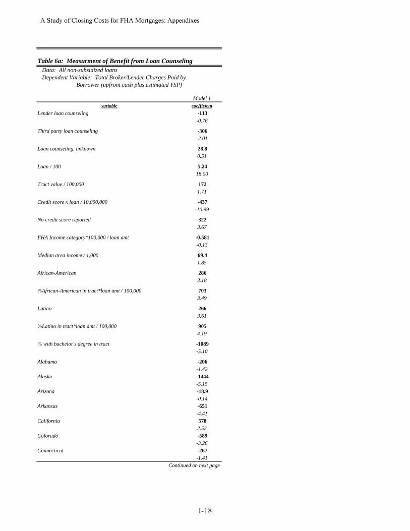
Table 6a: Measurment of Benefit from Loan Counseling Data: All non-subsidized loans Dependent Variable: Total Broker/Lender Charges Paid by Borrower (upfront cash plus estimated YSP)
Model 1variable coefficient
Lender loan counseling -113-0.76
Third party loan counseling -306-2.01
Loan counseling, unknown 28.80.51
Loan / 100 5.2418.00
Tract value / 100,000 1721.71
Credit score x loan / 10,000,000 -437-10.99
No credit score reported 3223.67
FHA Income category*100,000 / loan amt -0.581-0.13
Median area income / 1,000 69.41.85
African-American 2863.18
%African-American in tract*loan amt / 100,000 7033.49
Latino 2663.61
%Latino in tract*loan amt / 100,000 9054.19
% with bachelor's degree in tract -1089-5.10
Alabama -206-1.42
Alaska -1444-5.15
Arizona -18.9-0.14
Arkansas -651-4.41
California 5782.52
Colorado -589-3.26
Connecticut -267-1.41
Continued on next page
A Study of Closing Costs for FHA Mortgages: Appendixes
I-18
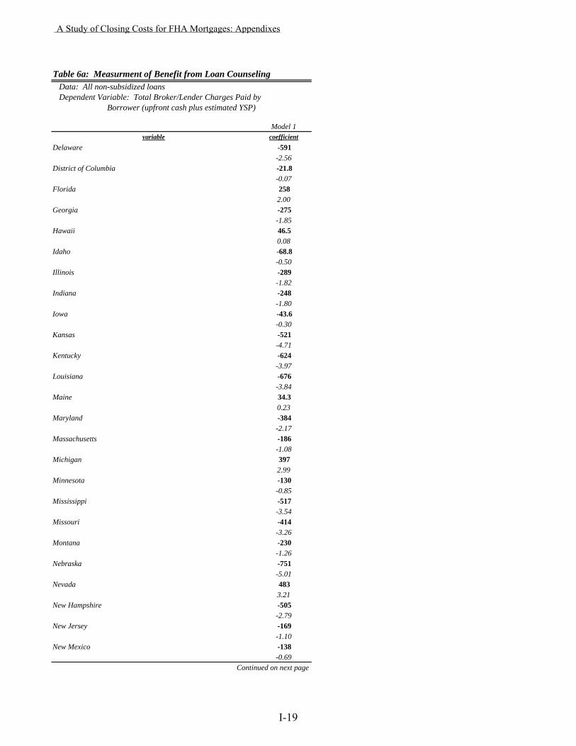
Table 6a: Measurment of Benefit from Loan Counseling Data: All non-subsidized loans Dependent Variable: Total Broker/Lender Charges Paid by Borrower (upfront cash plus estimated YSP)
Model 1variable coefficient
Delaware -591-2.56
District of Columbia -21.8-0.07
Florida 2582.00
Georgia -275-1.85
Hawaii 46.50.08
Idaho -68.8-0.50
Illinois -289-1.82
Indiana -248-1.80
Iowa -43.6-0.30
Kansas -521-4.71
Kentucky -624-3.97
Louisiana -676-3.84
Maine 34.30.23
Maryland -384-2.17
Massachusetts -186-1.08
Michigan 3972.99
Minnesota -130-0.85
Mississippi -517-3.54
Missouri -414-3.26
Montana -230-1.26
Nebraska -751-5.01
Nevada 4833.21
New Hampshire -505-2.79
New Jersey -169-1.10
New Mexico -138-0.69
Continued on next page
A Study of Closing Costs for FHA Mortgages: Appendixes
I-19
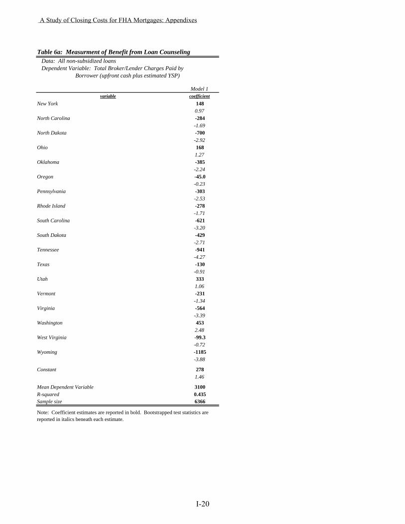
Table 6a: Measurment of Benefit from Loan Counseling Data: All non-subsidized loans Dependent Variable: Total Broker/Lender Charges Paid by Borrower (upfront cash plus estimated YSP)
Model 1variable coefficient
New York 1480.97
North Carolina -284-1.69
North Dakota -700-2.92
Ohio 1681.27
Oklahoma -385-2.24
Oregon -45.0-0.23
Pennsylvania -303-2.53
Rhode Island -278-1.71
South Carolina -621-3.20
South Dakota -429-2.71
Tennessee -941-4.27
Texas -130-0.91
Utah 3331.06
Vermont -231-1.34
Virginia -564-3.39
Washington 4532.48
West Virginia -99.3-0.72
Wyoming -1185-3.88
Constant 2781.46
Mean Dependent Variable 3100R-squared 0.435Sample size 6366
Note: Coefficient estimates are reported in bold. Bootstrapped test statistics are reported in italics beneath each estimate.
A Study of Closing Costs for FHA Mortgages: Appendixes
I-20
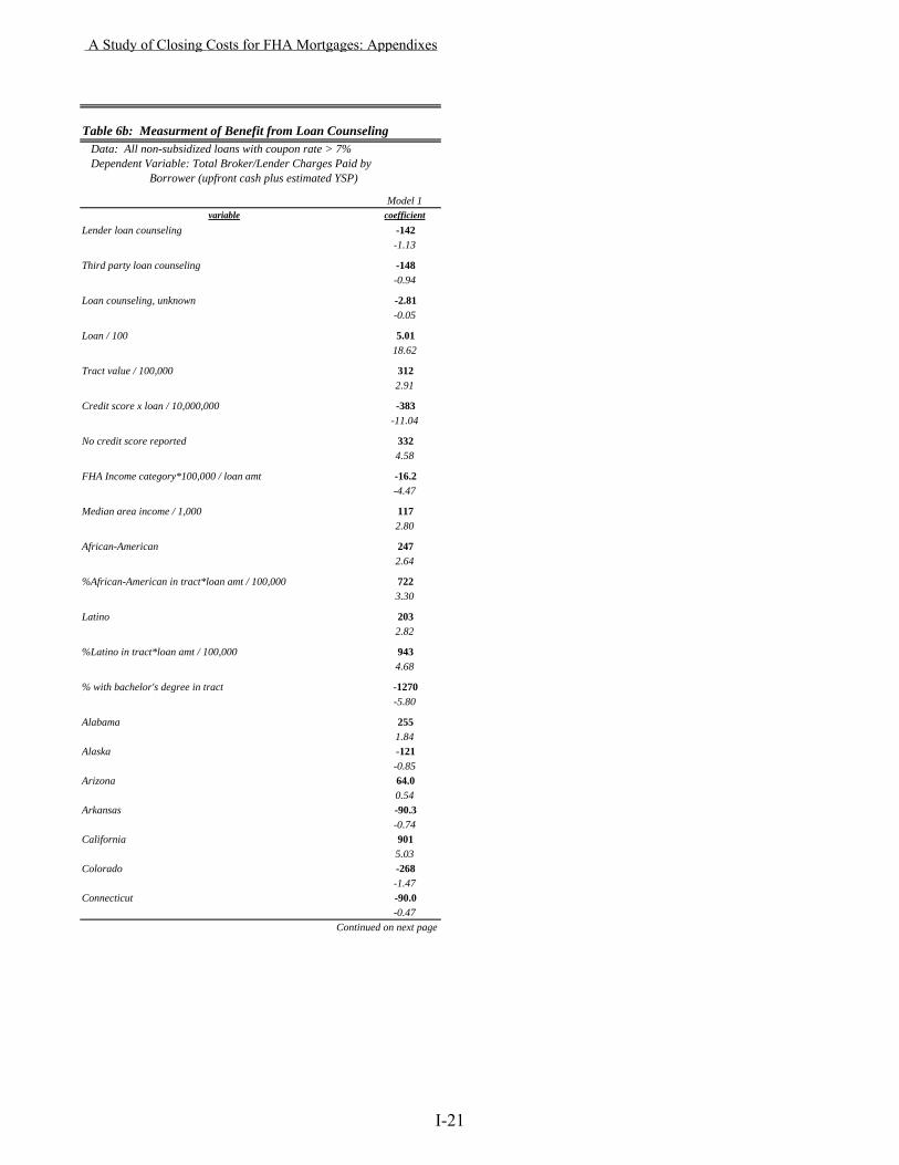
Table 6b: Measurment of Benefit from Loan Counseling Data: All non-subsidized loans with coupon rate > 7% Dependent Variable: Total Broker/Lender Charges Paid by Borrower (upfront cash plus estimated YSP)
Model 1variable coefficient
Lender loan counseling -142-1.13
Third party loan counseling -148-0.94
Loan counseling, unknown -2.81-0.05
Loan / 100 5.0118.62
Tract value / 100,000 3122.91
Credit score x loan / 10,000,000 -383-11.04
No credit score reported 3324.58
FHA Income category*100,000 / loan amt -16.2-4.47
Median area income / 1,000 1172.80
African-American 2472.64
%African-American in tract*loan amt / 100,000 7223.30
Latino 2032.82
%Latino in tract*loan amt / 100,000 9434.68
% with bachelor's degree in tract -1270-5.80
Alabama 2551.84
Alaska -121-0.85
Arizona 64.00.54
Arkansas -90.3-0.74
California 9015.03
Colorado -268-1.47
Connecticut -90.0-0.47
Continued on next page
A Study of Closing Costs for FHA Mortgages: Appendixes
I-21

Table 6b: Measurment of Benefit from Loan Counseling Data: All non-subsidized loans with coupon rate > 7% Dependent Variable: Total Broker/Lender Charges Paid by Borrower (upfront cash plus estimated YSP)
Model 1variable coefficient
Delaware -202-0.94
District of Columbia 1290.43
Florida 3322.87
Georgia 1401.02
Hawaii 9321.04
Idaho 1601.31
Illinois -127-1.02
Indiana 0.8930.01
Iowa 3152.50
Kansas -400-3.91
Kentucky -298-2.04
Louisiana -289-1.73
Maine 1981.52
Maryland -0.128NA
Massachusetts -208-1.22
Michigan 3783.06
Minnesota 3042.11
Mississippi -152-1.14
Missouri -308-2.77
Montana 2421.80
Nebraska -297-1.92
Nevada 5323.94
New Hampshire -203-1.42
New Jersey -158-0.94
New Mexico 3561.87
Continued on next page
A Study of Closing Costs for FHA Mortgages: Appendixes
I-22
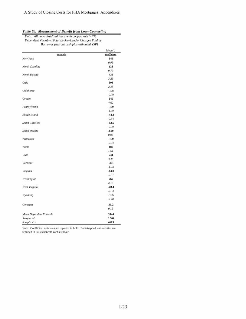
Table 6b: Measurment of Benefit from Loan Counseling Data: All non-subsidized loans with coupon rate > 7% Dependent Variable: Total Broker/Lender Charges Paid by Borrower (upfront cash plus estimated YSP)
Model 1variable coefficient
New York 1490.99
North Carolina 1380.79
North Dakota 4333.29
Ohio 3032.33
Oklahoma -108-0.70
Oregon 6454.62
Pennsylvania -179-1.59
Rhode Island -44.3-0.34
South Carolina -12.5-0.09
South Dakota 3.900.03
Tennessee -109-0.74
Texas 1821.51
Utah 7313.48
Vermont -321-1.74
Virginia -84.0-0.51
Washington 7674.16
West Virginia -40.4-0.33
Wyoming -105-0.78
Constant 36.20.19
Mean Dependent Variable 3544R-squared 0.564Sample size 4603
Note: Coefficient estimates are reported in bold. Bootstrapped test statistics are reported in italics beneath each estimate.
A Study of Closing Costs for FHA Mortgages: Appendixes
I-23
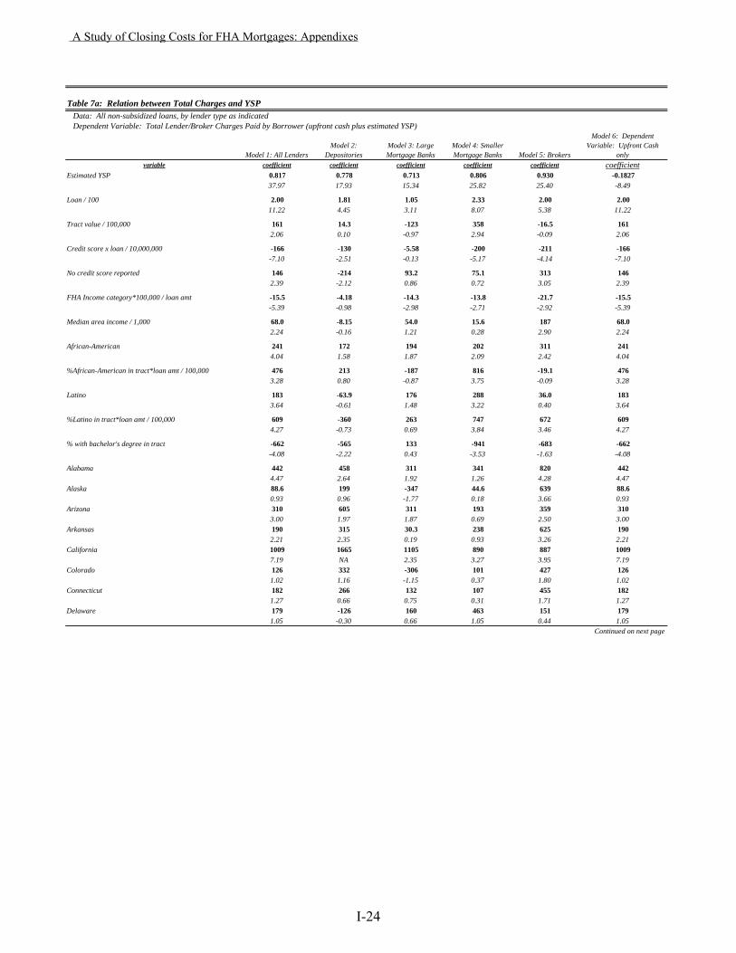
Table 7a: Relation between Total Charges and YSP Data: All non-subsidized loans, by lender type as indicated Dependent Variable: Total Lender/Broker Charges Paid by Borrower (upfront cash plus estimated YSP)
Model 1: All LendersModel 2:
DepositoriesModel 3: Large Mortgage Banks
Model 4: Smaller Mortgage Banks Model 5: Brokers
Model 6: Dependent Variable: Upfront Cash
onlyvariable coefficient coefficient coefficient coefficient coefficient coefficient
Estimated YSP 0.817 0.778 0.713 0.806 0.930 -0.182737.97 17.93 15.34 25.82 25.40 -8.49
Loan / 100 2.00 1.81 1.05 2.33 2.00 2.0011.22 4.45 3.11 8.07 5.38 11.22
Tract value / 100,000 161 14.3 -123 358 -16.5 1612.06 0.10 -0.97 2.94 -0.09 2.06
Credit score x loan / 10,000,000 -166 -130 -5.58 -200 -211 -166-7.10 -2.51 -0.13 -5.17 -4.14 -7.10
No credit score reported 146 -214 93.2 75.1 313 1462.39 -2.12 0.86 0.72 3.05 2.39
FHA Income category*100,000 / loan amt -15.5 -4.18 -14.3 -13.8 -21.7 -15.5-5.39 -0.98 -2.98 -2.71 -2.92 -5.39
Median area income / 1,000 68.0 -8.15 54.0 15.6 187 68.02.24 -0.16 1.21 0.28 2.90 2.24
African-American 241 172 194 202 311 2414.04 1.58 1.87 2.09 2.42 4.04
%African-American in tract*loan amt / 100,000 476 213 -187 816 -19.1 4763.28 0.80 -0.87 3.75 -0.09 3.28
Latino 183 -63.9 176 288 36.0 1833.64 -0.61 1.48 3.22 0.40 3.64
%Latino in tract*loan amt / 100,000 609 -360 263 747 672 6094.27 -0.73 0.69 3.84 3.46 4.27
% with bachelor's degree in tract -662 -565 133 -941 -683 -662-4.08 -2.22 0.43 -3.53 -1.63 -4.08
Alabama 442 458 311 341 820 4424.47 2.64 1.92 1.26 4.28 4.47
Alaska 88.6 199 -347 44.6 639 88.60.93 0.96 -1.77 0.18 3.66 0.93
Arizona 310 605 311 193 359 3103.00 1.97 1.87 0.69 2.50 3.00
Arkansas 190 315 30.3 238 625 1902.21 2.35 0.19 0.93 3.26 2.21
California 1009 1665 1105 890 887 10097.19 NA 2.35 3.27 3.95 7.19
Colorado 126 332 -306 101 427 1261.02 1.16 -1.15 0.37 1.80 1.02
Connecticut 182 266 132 107 455 1821.27 0.66 0.75 0.31 1.71 1.27
Delaware 179 -126 160 463 151 1791.05 -0.30 0.66 1.05 0.44 1.05
Continued on next page
A Study of Closing Costs for FHA Mortgages: Appendixes
I-24

Table 7a: Relation between Total Charges and YSP Data: All non-subsidized loans, by lender type as indicated Dependent Variable: Total Lender/Broker Charges Paid by Borrower (upfront cash plus estimated YSP)
Model 1: All LendersModel 2:
DepositoriesModel 3: Large Mortgage Banks
Model 4: Smaller Mortgage Banks Model 5: Brokers
Model 6: Dependent Variable: Upfront Cash
onlyvariable coefficient coefficient coefficient coefficient coefficient coefficient
District of Columbia 789 514 1657 494 1436 7893.43 0.56 3.14 1.40 3.56 3.43
Florida 444 356 -128 440 669 4444.33 2.09 -0.84 1.57 4.35 4.33
Georgia 429 456 312 277 841 4294.74 2.64 2.23 1.11 5.24 4.74
Hawaii 1158 645 1214 1346 -142 11582.79 0.93 1.21 2.29 NA 2.79
Idaho 439 498 326 462 586 4394.51 3.62 2.42 1.54 2.66 4.51
Illinois -67.6 -86.9 -179 81.3 75.4 -67.6-0.63 -0.26 -1.17 0.30 0.46 -0.63
Indiana 71.9 401 -412 49.9 434 71.90.74 1.70 -3.29 0.20 2.55 0.74
Iowa 464 356 9.72 827 702 4644.63 2.26 0.08 2.69 3.40 4.63
Kansas -213 -71.1 -524 -180 216 -213-2.42 -0.51 -4.29 -0.66 1.40 -2.42
Kentucky 117 -165 -185 633 496 1171.15 -1.14 -1.36 2.04 3.13 1.15
Louisiana 71.1 171 7.76 -54.7 571 71.10.64 1.11 0.03 -0.20 3.11 0.64
Maine 444 264 268 526 106 4443.86 0.67 1.66 1.82 0.38 3.86
Maryland 287 708 361 131 550 2872.48 3.36 2.09 0.45 2.00 2.48
Massachusetts -307 21.0 -419 -224 -200 -307-2.53 0.08 -2.04 -0.75 -0.97 -2.53
Michigan 368 587 -398 676 379 3683.62 2.94 -2.49 2.60 2.34 3.62
Minnesota 631 708 720 578 527 6316.43 4.30 3.43 2.24 2.65 6.43
Mississippi 157 174 112 326 859 1571.56 1.15 0.70 1.08 2.97 1.56
Missouri -181 -131 -435 -184 340 -181-1.94 -0.96 -3.13 -0.70 1.65 -1.94
Montana 517 862 182 398 518 5174.70 4.30 0.83 1.49 3.19 4.70
Nebraska -150 11.7 -282 -276 531 -150-1.62 0.08 -1.86 -1.06 1.89 -1.62
Nevada 614 829 137 790 695 6145.34 3.87 0.89 2.83 4.08 5.34
New Hampshire -203 -531 -166 -63.5 -435 -203-1.75 -2.38 -1.08 -0.20 -1.77 -1.75
New Jersey -20.5 4.52 -404 67.7 204 -20.5-0.16 0.02 -2.08 0.24 0.99 -0.16
New Mexico 574 630 508 1131 937 5743.72 2.50 1.89 2.81 3.10 3.72
Continued on next page
A Study of Closing Costs for FHA Mortgages: Appendixes
I-25
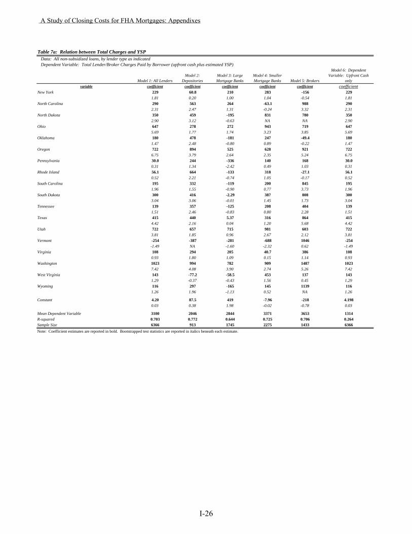
Table 7a: Relation between Total Charges and YSP Data: All non-subsidized loans, by lender type as indicated Dependent Variable: Total Lender/Broker Charges Paid by Borrower (upfront cash plus estimated YSP)
Model 1: All LendersModel 2:
DepositoriesModel 3: Large Mortgage Banks
Model 4: Smaller Mortgage Banks Model 5: Brokers
Model 6: Dependent Variable: Upfront Cash
onlyvariable coefficient coefficient coefficient coefficient coefficient coefficient
New York 229 60.8 210 283 -156 2291.81 0.20 1.00 1.04 -0.54 1.81
North Carolina 290 563 264 -63.1 988 2902.31 2.47 1.31 -0.24 3.32 2.31
North Dakota 350 459 -195 831 780 3502.90 3.12 -0.63 NA NA 2.90
Ohio 647 278 272 943 719 6475.69 1.77 1.74 3.23 3.85 5.69
Oklahoma 180 478 -181 247 -49.4 1801.47 2.48 -0.80 0.89 -0.22 1.47
Oregon 722 894 525 628 921 7226.75 3.79 2.64 2.35 5.24 6.75
Pennsylvania 30.0 244 -336 140 168 30.00.31 1.34 -2.42 0.49 1.03 0.31
Rhode Island 56.1 664 -133 318 -27.1 56.10.52 2.21 -0.74 1.05 -0.17 0.52
South Carolina 195 332 -119 200 845 1951.96 1.55 -0.90 0.77 3.73 1.96
South Dakota 300 416 -2.29 387 808 3003.04 3.06 -0.01 1.45 1.73 3.04
Tennessee 139 357 -125 208 404 1391.51 2.46 -0.83 0.80 2.28 1.51
Texas 415 440 5.37 316 864 4154.42 2.16 0.04 1.20 5.68 4.42
Utah 722 657 715 981 603 7223.81 1.85 0.96 2.67 2.12 3.81
Vermont -254 -387 -281 -688 1046 -254-1.49 NA -1.60 -2.32 0.62 -1.49
Virginia 108 294 205 40.7 386 1080.93 1.80 1.09 0.15 1.14 0.93
Washington 1023 994 782 909 1487 10237.42 4.08 3.90 2.74 5.26 7.42
West Virginia 143 -77.2 -58.5 453 137 1431.29 -0.37 -0.43 1.56 0.45 1.29
Wyoming 116 297 -165 145 1139 1161.26 1.96 -1.13 0.52 NA 1.26
Constant 4.20 87.5 419 -7.96 -218 4.1980.03 0.38 1.98 -0.02 -0.78 0.03
Mean Dependent Variable 3100 2046 2844 3371 3653 1314R-squared 0.703 0.772 0.644 0.725 0.706 0.264Sample Size 6366 913 1745 2275 1433 6366Note: Coefficient estimates are reported in bold. Bootstrapped test statistics are reported in italics beneath each estimate.
A Study of Closing Costs for FHA Mortgages: Appendixes
I-26
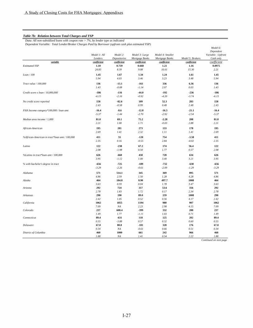
Table 7b: Relation between Total Charges and YSP Data: All non-subsidized loans with coupon rate > 7%, by lender type as indicated Dependent Variable: Total Lender/Broker Charges Paid by Borrower (upfront cash plus estimated YSP)
Model 1: All Lenders
Model 2: Depositories
Model 3: Large Mortgage Banks
Model 4: Smaller Mortgage Banks Model 5: Brokers
Model 6: Dependent
Variable: Upfront Cash only
variable coefficient coefficient coefficient coefficient coefficient coefficientEstimated YSP 1.10 0.759 0.668 1.21 1.16 0.0975
24.83 8.39 9.08 16.61 15.30 2.21
Loan / 100 1.45 1.67 1.34 1.24 1.61 1.455.94 4.03 3.46 3.23 3.48 5.94
Tract value / 100,000 136 -13.1 -161 336 6.36 1361.43 -0.08 -1.14 2.07 0.03 1.43
Credit score x loan / 10,000,000 -186 -116 -44.0 -192 -236 -186-6.15 -2.16 -0.92 -4.20 -3.74 -6.15
No credit score reported 158 -82.6 109 52.3 283 1582.43 -0.58 0.99 0.48 2.48 2.43
FHA Income category*100,000 / loan amt -16.4 -8.6 -12.8 -16.3 -21.1 -16.4-5.37 -1.44 -2.70 -2.92 -2.54 -5.37
Median area income / 1,000 81.0 69.1 75.2 -2.28 208 81.02.21 1.00 1.71 -0.03 2.88 2.21
African-American 195 201 273 133 178 1952.69 1.41 2.32 1.11 1.41 2.69
%African-American in tract*loan amt / 100,000 411 55 -120 754 -3.58 4112.35 0.16 -0.55 2.84 -0.02 2.35
Latino 122 -238 67.2 174 56.4 1222.08 -1.98 0.50 1.77 0.57 2.08
%Latino in tract*loan amt / 100,000 626 -660 458 728 634 6263.95 -1.12 1.00 3.40 3.21 3.95
% with bachelor's degree in tract -656 -725 -189 -732 -630 -656-3.29 -2.26 -0.61 -2.09 -1.29 -3.29
Alabama 571 514.1 345 369 895 5714.86 2.59 1.50 1.28 4.28 4.86
Alaska 464 184.8 8.90 497.7 1008 4643.63 0.59 0.04 1.78 3.47 3.63
Arizona 292 724 317 53.6 356 2922.78 1.83 1.72 0.17 2.34 2.78
Arkansas 290 190 89.0 159 1008 2902.42 1.05 0.52 0.56 4.17 2.42
California 1062 1855 1194 980 907 10627.09 NA 2.23 2.98 4.15 7.09
Colorado 237 608.4 -399 332 288 2371.49 1.77 -1.11 1.03 0.71 1.49
Connecticut 89.4 -631 118 125 202 89.40.55 -3.88 0.57 0.32 0.60 0.55
Delaware 67.0 80.8 -181 328 176 67.00.34 NA -0.61 0.66 0.51 0.34
District of Columbia 460 1000 661 242 966 4601.88 NA 1.41 0.54 2.22 1.88
Continued on next page
A Study of Closing Costs for FHA Mortgages: Appendixes
I-27
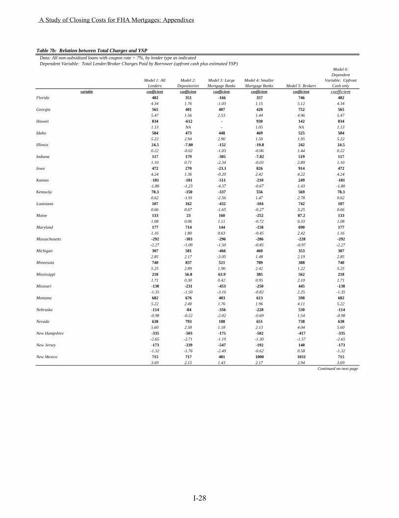
Table 7b: Relation between Total Charges and YSP Data: All non-subsidized loans with coupon rate > 7%, by lender type as indicated Dependent Variable: Total Lender/Broker Charges Paid by Borrower (upfront cash plus estimated YSP)
Model 1: All Lenders
Model 2: Depositories
Model 3: Large Mortgage Banks
Model 4: Smaller Mortgage Banks Model 5: Brokers
Model 6: Dependent
Variable: Upfront Cash only
variable coefficient coefficient coefficient coefficient coefficient coefficientFlorida 482 351 -166 357 746 482
4.34 1.76 -1.03 1.15 5.12 4.34Georgia 565 401 407 420 752 565
5.47 1.56 2.53 1.44 4.96 5.47Hawaii 834 -612 - 930 142 834
1.13 NA - 1.05 NA 1.13Idaho 584 473 448 469 525 584
5.22 2.94 2.90 1.50 1.95 5.22Illinois 24.5 -7.80 -152 -19.8 242 24.5
0.22 -0.02 -1.03 -0.06 1.44 0.22Indiana 117 179 -305 -7.82 519 117
1.10 0.71 -2.34 -0.03 2.89 1.10Iowa 472 270 -23.1 826 914 472
4.24 1.36 -0.20 2.42 4.22 4.24Kansas -181 -181 -511 -210 249 -181
-1.80 -1.23 -4.37 -0.67 1.43 -1.80Kentucky 78.3 -350 -337 556 569 78.3
0.62 -1.91 -2.56 1.47 2.78 0.62Louisiana 107 162 -432 -104 742 107
0.66 0.67 -1.65 -0.27 3.25 0.66Maine 133 23 160 -252 87.2 133
1.08 0.06 1.11 -0.72 0.33 1.08Maryland 177 714 144 -158 690 177
1.16 1.80 0.63 -0.45 2.42 1.16Massachusetts -292 -303 -296 -286 -228 -292
-2.27 -1.09 -1.50 -0.85 -0.97 -2.27Michigan 307 581 -466 460 353 307
2.85 2.17 -3.05 1.48 2.19 2.85Minnesota 740 837 521 789 388 740
5.25 2.89 1.90 2.42 1.22 5.25Mississippi 218 56.8 63.9 385 562 218
1.71 0.30 0.42 0.95 2.10 1.71Missouri -138 -231 -453 -250 445 -138
-1.35 -1.50 -3.16 -0.82 2.25 -1.35Montana 682 676 403 613 598 682
5.22 2.40 1.76 1.96 4.11 5.22Nebraska -114 -84 -356 -228 530 -114
-0.98 -0.52 -2.02 -0.69 1.54 -0.98Nevada 638 793 188 651 738 638
5.60 2.58 1.18 2.13 4.04 5.60New Hampshire -335 -503 -175 -502 -417 -335
-2.65 -2.71 -1.19 -1.30 -1.57 -2.65New Jersey -173 -339 -547 -192 140 -173
-1.32 -1.76 -2.49 -0.62 0.58 -1.32New Mexico 715 717 481 1000 1031 715
3.69 2.15 1.43 2.17 2.94 3.69Continued on next page
A Study of Closing Costs for FHA Mortgages: Appendixes
I-28
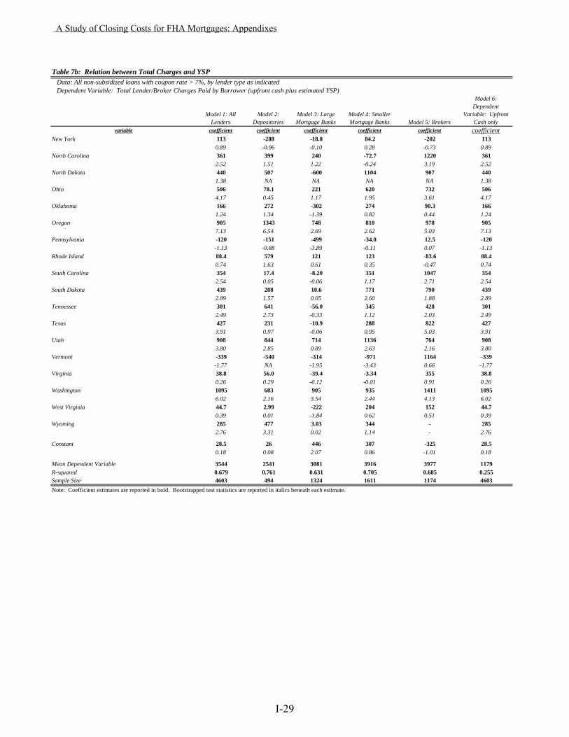
Table 7b: Relation between Total Charges and YSP Data: All non-subsidized loans with coupon rate > 7%, by lender type as indicated Dependent Variable: Total Lender/Broker Charges Paid by Borrower (upfront cash plus estimated YSP)
Model 1: All Lenders
Model 2: Depositories
Model 3: Large Mortgage Banks
Model 4: Smaller Mortgage Banks Model 5: Brokers
Model 6: Dependent
Variable: Upfront Cash only
variable coefficient coefficient coefficient coefficient coefficient coefficientNew York 113 -288 -18.8 84.2 -202 113
0.89 -0.96 -0.10 0.28 -0.73 0.89North Carolina 361 399 240 -72.7 1220 361
2.52 1.51 1.22 -0.24 3.19 2.52North Dakota 440 507 -600 1104 907 440
1.38 NA NA NA NA 1.38Ohio 506 78.1 221 620 732 506
4.17 0.45 1.17 1.95 3.61 4.17Oklahoma 166 272 -302 274 90.3 166
1.24 1.34 -1.39 0.82 0.44 1.24Oregon 905 1343 748 810 978 905
7.13 6.54 2.69 2.62 5.03 7.13Pennsylvania -120 -151 -499 -34.0 12.5 -120
-1.13 -0.88 -3.89 -0.11 0.07 -1.13Rhode Island 88.4 579 121 123 -83.6 88.4
0.74 1.63 0.61 0.35 -0.47 0.74South Carolina 354 17.4 -8.20 351 1047 354
2.54 0.05 -0.06 1.17 2.71 2.54South Dakota 439 288 10.6 771 790 439
2.89 1.57 0.05 2.60 1.88 2.89Tennessee 301 641 -56.0 345 428 301
2.49 2.73 -0.33 1.12 2.03 2.49Texas 427 231 -10.9 288 822 427
3.91 0.97 -0.06 0.95 5.03 3.91Utah 908 844 714 1136 764 908
3.80 2.85 0.89 2.63 2.16 3.80Vermont -339 -540 -314 -971 1164 -339
-1.77 NA -1.95 -3.43 0.66 -1.77Virginia 38.8 56.0 -39.4 -3.34 355 38.8
0.26 0.29 -0.12 -0.01 0.91 0.26Washington 1095 683 905 935 1411 1095
6.02 2.16 3.54 2.44 4.13 6.02West Virginia 44.7 2.99 -222 204 152 44.7
0.39 0.01 -1.84 0.62 0.51 0.39Wyoming 285 477 3.03 344 - 285
2.76 3.31 0.02 1.14 - 2.76
Constant 28.5 26 446 307 -325 28.50.18 0.08 2.07 0.86 -1.01 0.18
Mean Dependent Variable 3544 2541 3081 3916 3977 1179R-squared 0.679 0.761 0.631 0.705 0.685 0.255Sample Size 4603 494 1324 1611 1174 4603Note: Coefficient estimates are reported in bold. Bootstrapped test statistics are reported in italics beneath each estimate.
A Study of Closing Costs for FHA Mortgages: Appendixes
I-29
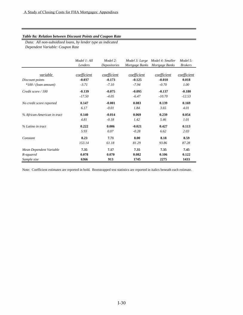
Table 8a: Relation between Discount Points and Coupon Rate Data: All non-subsidized loans, by lender type as indicated Dependent Variable: Coupon Rate
Model 1: All Lenders
Model 2: Depositories
Model 3: Large Mortgage Banks
Model 4: Smaller Mortgage Banks
Model 5: Brokers
variable coefficient coefficient coefficient coefficient coefficientDiscount points -0.037 -0.173 -0.125 -0.010 0.018 *100 / (loan amount) -3.71 -7.10 -7.94 -0.70 1.00
Credit score / 100 -0.139 -0.075 -0.095 -0.137 -0.180-17.50 -4.05 -6.47 -10.70 -12.53
No credit score reported 0.147 -0.001 0.083 0.139 0.1696.17 -0.01 1.84 3.65 4.01
% African-American in tract 0.140 -0.014 0.069 0.239 0.0544.81 -0.18 1.42 5.46 1.01
% Latino in tract 0.222 0.006 -0.021 0.427 0.1135.93 0.07 -0.28 6.62 2.03
Constant 8.23 7.71 8.00 8.18 8.59153.14 61.18 81.29 93.86 87.28
Mean Dependent Variable 7.35 7.17 7.35 7.35 7.45R-squared 0.078 0.070 0.082 0.106 0.122Sample size 6366 913 1745 2275 1433
Note: Coefficient estimates are reported in bold. Bootstrapped test statistics are reported in italics beneath each estimate.
A Study of Closing Costs for FHA Mortgages: Appendixes
I-30
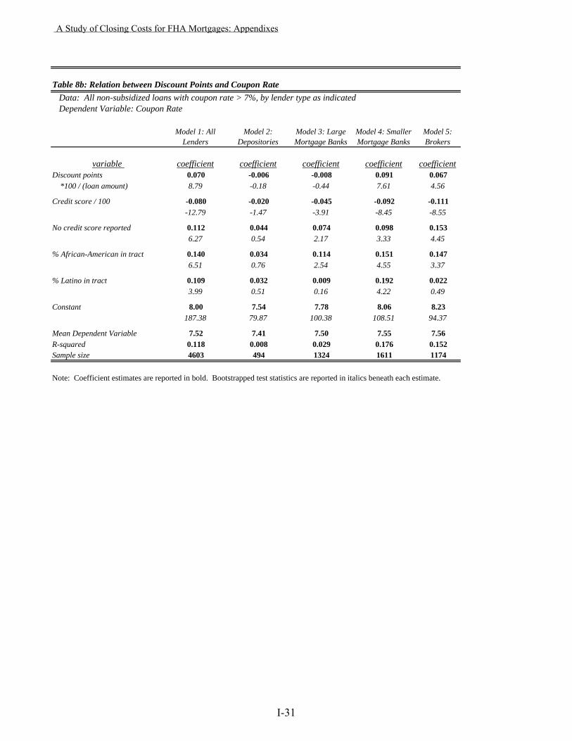
Table 8b: Relation between Discount Points and Coupon Rate Data: All non-subsidized loans with coupon rate > 7%, by lender type as indicated Dependent Variable: Coupon Rate
Model 1: All Lenders
Model 2: Depositories
Model 3: Large Mortgage Banks
Model 4: Smaller Mortgage Banks
Model 5: Brokers
variable coefficient coefficient coefficient coefficient coefficientDiscount points 0.070 -0.006 -0.008 0.091 0.067 *100 / (loan amount) 8.79 -0.18 -0.44 7.61 4.56
Credit score / 100 -0.080 -0.020 -0.045 -0.092 -0.111-12.79 -1.47 -3.91 -8.45 -8.55
No credit score reported 0.112 0.044 0.074 0.098 0.1536.27 0.54 2.17 3.33 4.45
% African-American in tract 0.140 0.034 0.114 0.151 0.1476.51 0.76 2.54 4.55 3.37
% Latino in tract 0.109 0.032 0.009 0.192 0.0223.99 0.51 0.16 4.22 0.49
Constant 8.00 7.54 7.78 8.06 8.23187.38 79.87 100.38 108.51 94.37
Mean Dependent Variable 7.52 7.41 7.50 7.55 7.56R-squared 0.118 0.008 0.029 0.176 0.152Sample size 4603 494 1324 1611 1174
Note: Coefficient estimates are reported in bold. Bootstrapped test statistics are reported in italics beneath each estimate.
A Study of Closing Costs for FHA Mortgages: Appendixes
I-31
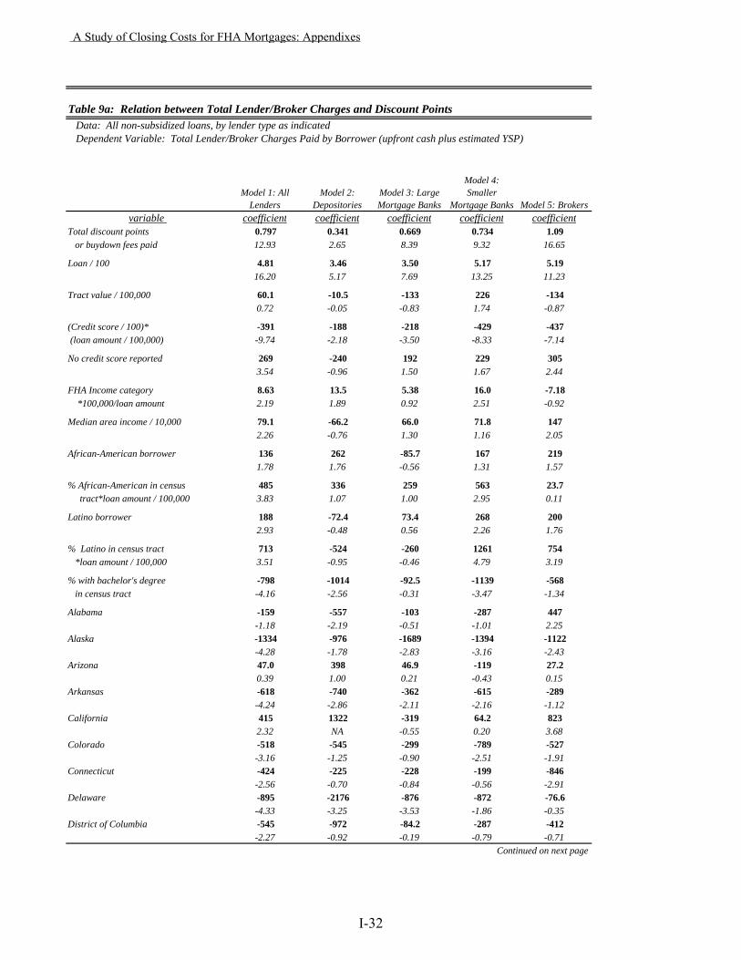
Table 9a: Relation between Total Lender/Broker Charges and Discount Points Data: All non-subsidized loans, by lender type as indicated Dependent Variable: Total Lender/Broker Charges Paid by Borrower (upfront cash plus estimated YSP)
Model 1: All Lenders
Model 2: Depositories
Model 3: Large Mortgage Banks
Model 4: Smaller
Mortgage Banks Model 5: Brokersvariable coefficient coefficient coefficient coefficient coefficient
Total discount points 0.797 0.341 0.669 0.734 1.09 or buydown fees paid 12.93 2.65 8.39 9.32 16.65
Loan / 100 4.81 3.46 3.50 5.17 5.1916.20 5.17 7.69 13.25 11.23
Tract value / 100,000 60.1 -10.5 -133 226 -1340.72 -0.05 -0.83 1.74 -0.87
(Credit score / 100)* -391 -188 -218 -429 -437 (loan amount / 100,000) -9.74 -2.18 -3.50 -8.33 -7.14
No credit score reported 269 -240 192 229 3053.54 -0.96 1.50 1.67 2.44
FHA Income category 8.63 13.5 5.38 16.0 -7.18 *100,000/loan amount 2.19 1.89 0.92 2.51 -0.92
Median area income / 10,000 79.1 -66.2 66.0 71.8 1472.26 -0.76 1.30 1.16 2.05
African-American borrower 136 262 -85.7 167 2191.78 1.76 -0.56 1.31 1.57
% African-American in census 485 336 259 563 23.7 tract*loan amount / 100,000 3.83 1.07 1.00 2.95 0.11
Latino borrower 188 -72.4 73.4 268 200 2.93 -0.48 0.56 2.26 1.76
% Latino in census tract 713 -524 -260 1261 754 *loan amount / 100,000 3.51 -0.95 -0.46 4.79 3.19
% with bachelor's degree -798 -1014 -92.5 -1139 -568 in census tract -4.16 -2.56 -0.31 -3.47 -1.34
Alabama -159 -557 -103 -287 447-1.18 -2.19 -0.51 -1.01 2.25
Alaska -1334 -976 -1689 -1394 -1122-4.28 -1.78 -2.83 -3.16 -2.43
Arizona 47.0 398 46.9 -119 27.20.39 1.00 0.21 -0.43 0.15
Arkansas -618 -740 -362 -615 -289-4.24 -2.86 -2.11 -2.16 -1.12
California 415 1322 -319 64.2 8232.32 NA -0.55 0.20 3.68
Colorado -518 -545 -299 -789 -527-3.16 -1.25 -0.90 -2.51 -1.91
Connecticut -424 -225 -228 -199 -846-2.56 -0.70 -0.84 -0.56 -2.91
Delaware -895 -2176 -876 -872 -76.6-4.33 -3.25 -3.53 -1.86 -0.35
District of Columbia -545 -972 -84.2 -287 -412-2.27 -0.92 -0.19 -0.79 -0.71
Continued on next page
A Study of Closing Costs for FHA Mortgages: Appendixes
I-32
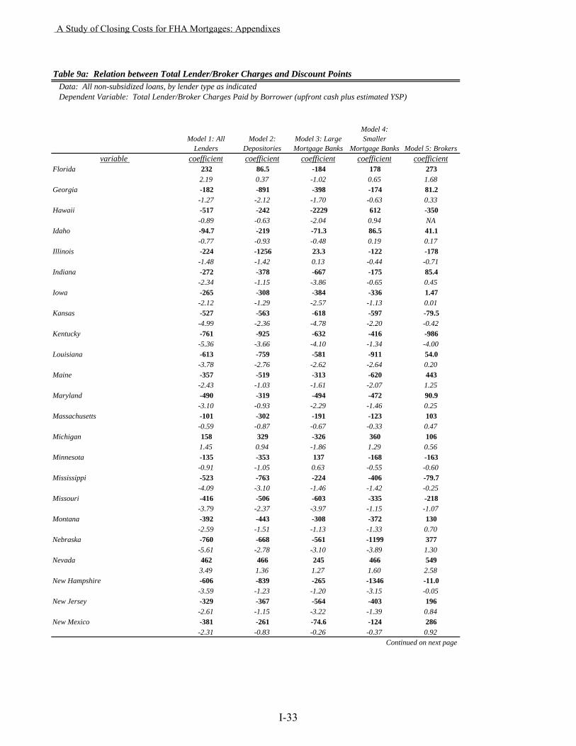
Table 9a: Relation between Total Lender/Broker Charges and Discount Points Data: All non-subsidized loans, by lender type as indicated Dependent Variable: Total Lender/Broker Charges Paid by Borrower (upfront cash plus estimated YSP)
Model 1: All Lenders
Model 2: Depositories
Model 3: Large Mortgage Banks
Model 4: Smaller
Mortgage Banks Model 5: Brokersvariable coefficient coefficient coefficient coefficient coefficient
Florida 232 86.5 -184 178 2732.19 0.37 -1.02 0.65 1.68
Georgia -182 -891 -398 -174 81.2-1.27 -2.12 -1.70 -0.63 0.33
Hawaii -517 -242 -2229 612 -350-0.89 -0.63 -2.04 0.94 NA
Idaho -94.7 -219 -71.3 86.5 41.1-0.77 -0.93 -0.48 0.19 0.17
Illinois -224 -1256 23.3 -122 -178-1.48 -1.42 0.13 -0.44 -0.71
Indiana -272 -378 -667 -175 85.4-2.34 -1.15 -3.86 -0.65 0.45
Iowa -265 -308 -384 -336 1.47-2.12 -1.29 -2.57 -1.13 0.01
Kansas -527 -563 -618 -597 -79.5-4.99 -2.36 -4.78 -2.20 -0.42
Kentucky -761 -925 -632 -416 -986-5.36 -3.66 -4.10 -1.34 -4.00
Louisiana -613 -759 -581 -911 54.0-3.78 -2.76 -2.62 -2.64 0.20
Maine -357 -519 -313 -620 443-2.43 -1.03 -1.61 -2.07 1.25
Maryland -490 -319 -494 -472 90.9-3.10 -0.93 -2.29 -1.46 0.25
Massachusetts -101 -302 -191 -123 103-0.59 -0.87 -0.67 -0.33 0.47
Michigan 158 329 -326 360 1061.45 0.94 -1.86 1.29 0.56
Minnesota -135 -353 137 -168 -163-0.91 -1.05 0.63 -0.55 -0.60
Mississippi -523 -763 -224 -406 -79.7-4.09 -3.10 -1.46 -1.42 -0.25
Missouri -416 -506 -603 -335 -218-3.79 -2.37 -3.97 -1.15 -1.07
Montana -392 -443 -308 -372 130-2.59 -1.51 -1.13 -1.33 0.70
Nebraska -760 -668 -561 -1199 377-5.61 -2.78 -3.10 -3.89 1.30
Nevada 462 466 245 466 5493.49 1.36 1.27 1.60 2.58
New Hampshire -606 -839 -265 -1346 -11.0-3.59 -1.23 -1.20 -3.15 -0.05
New Jersey -329 -367 -564 -403 196-2.61 -1.15 -3.22 -1.39 0.84
New Mexico -381 -261 -74.6 -124 286-2.31 -0.83 -0.26 -0.37 0.92
Continued on next page
A Study of Closing Costs for FHA Mortgages: Appendixes
I-33
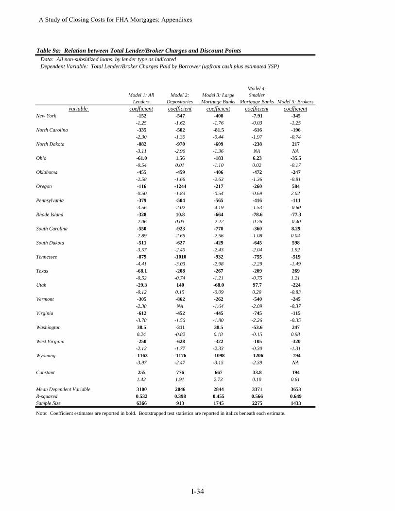
Table 9a: Relation between Total Lender/Broker Charges and Discount Points Data: All non-subsidized loans, by lender type as indicated Dependent Variable: Total Lender/Broker Charges Paid by Borrower (upfront cash plus estimated YSP)
Model 1: All Lenders
Model 2: Depositories
Model 3: Large Mortgage Banks
Model 4: Smaller
Mortgage Banks Model 5: Brokersvariable coefficient coefficient coefficient coefficient coefficient
New York -152 -547 -408 -7.91 -345-1.25 -1.62 -1.76 -0.03 -1.25
North Carolina -335 -502 -81.5 -616 -196-2.30 -1.30 -0.44 -1.97 -0.74
North Dakota -882 -970 -609 -238 217-3.11 -2.96 -1.36 NA NA
Ohio -61.0 1.56 -183 6.23 -35.5-0.54 0.01 -1.10 0.02 -0.17
Oklahoma -455 -459 -406 -472 -247-2.58 -1.66 -2.63 -1.36 -0.81
Oregon -116 -1244 -217 -260 584-0.50 -1.83 -0.54 -0.69 2.02
Pennsylvania -379 -504 -565 -416 -111-3.56 -2.02 -4.19 -1.53 -0.60
Rhode Island -328 10.8 -664 -78.6 -77.3-2.06 0.03 -2.22 -0.26 -0.40
South Carolina -550 -923 -770 -360 8.29-2.89 -2.65 -2.56 -1.08 0.04
South Dakota -511 -627 -429 -645 598-3.57 -2.40 -2.43 -2.04 1.92
Tennessee -879 -1010 -932 -755 -519-4.41 -3.03 -2.98 -2.29 -1.49
Texas -68.1 -208 -267 -209 269-0.52 -0.74 -1.21 -0.75 1.21
Utah -29.3 140 -68.0 97.7 -224-0.12 0.15 -0.09 0.20 -0.83
Vermont -305 -862 -262 -540 -245-2.38 NA -1.64 -2.09 -0.37
Virginia -612 -452 -445 -745 -115-3.78 -1.56 -1.80 -2.26 -0.35
Washington 38.5 -311 38.5 -53.6 2470.24 -0.82 0.18 -0.15 0.98
West Virginia -250 -628 -322 -105 -320-2.12 -1.77 -2.33 -0.30 -1.31
Wyoming -1163 -1176 -1098 -1206 -794-3.97 -2.47 -3.15 -2.39 NA
Constant 255 776 667 33.8 1941.42 1.91 2.73 0.10 0.61
Mean Dependent Variable 3100 2046 2844 3371 3653R-squared 0.532 0.398 0.455 0.566 0.649Sample Size 6366 913 1745 2275 1433
Note: Coefficient estimates are reported in bold. Bootstrapped test statistics are reported in italics beneath each estimate.
A Study of Closing Costs for FHA Mortgages: Appendixes
I-34
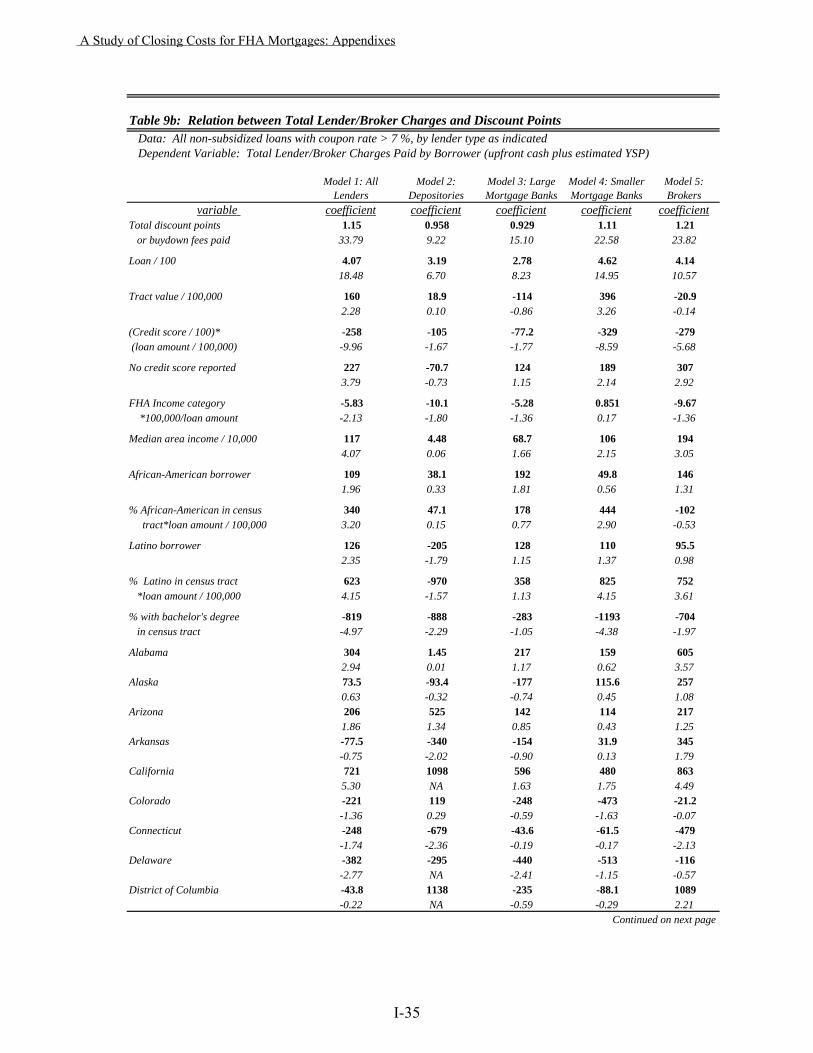
Table 9b: Relation between Total Lender/Broker Charges and Discount Points Data: All non-subsidized loans with coupon rate > 7 %, by lender type as indicated Dependent Variable: Total Lender/Broker Charges Paid by Borrower (upfront cash plus estimated YSP)
Model 1: All Lenders
Model 2: Depositories
Model 3: Large Mortgage Banks
Model 4: Smaller Mortgage Banks
Model 5: Brokers
variable coefficient coefficient coefficient coefficient coefficientTotal discount points 1.15 0.958 0.929 1.11 1.21 or buydown fees paid 33.79 9.22 15.10 22.58 23.82
Loan / 100 4.07 3.19 2.78 4.62 4.1418.48 6.70 8.23 14.95 10.57
Tract value / 100,000 160 18.9 -114 396 -20.92.28 0.10 -0.86 3.26 -0.14
(Credit score / 100)* -258 -105 -77.2 -329 -279 (loan amount / 100,000) -9.96 -1.67 -1.77 -8.59 -5.68
No credit score reported 227 -70.7 124 189 3073.79 -0.73 1.15 2.14 2.92
FHA Income category -5.83 -10.1 -5.28 0.851 -9.67 *100,000/loan amount -2.13 -1.80 -1.36 0.17 -1.36
Median area income / 10,000 117 4.48 68.7 106 1944.07 0.06 1.66 2.15 3.05
African-American borrower 109 38.1 192 49.8 1461.96 0.33 1.81 0.56 1.31
% African-American in census 340 47.1 178 444 -102 tract*loan amount / 100,000 3.20 0.15 0.77 2.90 -0.53
Latino borrower 126 -205 128 110 95.5 2.35 -1.79 1.15 1.37 0.98
% Latino in census tract 623 -970 358 825 752 *loan amount / 100,000 4.15 -1.57 1.13 4.15 3.61
% with bachelor's degree -819 -888 -283 -1193 -704 in census tract -4.97 -2.29 -1.05 -4.38 -1.97
Alabama 304 1.45 217 159 6052.94 0.01 1.17 0.62 3.57
Alaska 73.5 -93.4 -177 115.6 2570.63 -0.32 -0.74 0.45 1.08
Arizona 206 525 142 114 2171.86 1.34 0.85 0.43 1.25
Arkansas -77.5 -340 -154 31.9 345-0.75 -2.02 -0.90 0.13 1.79
California 721 1098 596 480 8635.30 NA 1.63 1.75 4.49
Colorado -221 119 -248 -473 -21.2-1.36 0.29 -0.59 -1.63 -0.07
Connecticut -248 -679 -43.6 -61.5 -479-1.74 -2.36 -0.19 -0.17 -2.13
Delaware -382 -295 -440 -513 -116-2.77 NA -2.41 -1.15 -0.57
District of Columbia -43.8 1138 -235 -88.1 1089-0.22 NA -0.59 -0.29 2.21
Continued on next page
A Study of Closing Costs for FHA Mortgages: Appendixes
I-35
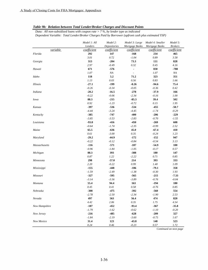
Table 9b: Relation between Total Lender/Broker Charges and Discount Points Data: All non-subsidized loans with coupon rate > 7 %, by lender type as indicated Dependent Variable: Total Lender/Broker Charges Paid by Borrower (upfront cash plus estimated YSP)
Model 1: All Lenders
Model 2: Depositories
Model 3: Large Mortgage Banks
Model 4: Smaller Mortgage Banks
Model 5: Brokers
variable coefficient coefficient coefficient coefficient coefficientFlorida 292 147 -168 234 465
3.01 0.72 -1.04 0.89 3.58Georgia 313 -204 73.3 111 828
2.97 -0.49 0.32 0.45 4.16Hawaii 671 -576 - 830 -788
1.07 NA - 1.07 NAIdaho 118 5.2 71.2 323 351
1.13 0.03 0.56 0.83 1.66Illinois -27.1 -199 -8.26 -94.6 75.4
-0.26 -0.34 -0.05 -0.36 0.42Indiana -20.2 -16.5 -278 -37.9 166
-0.22 -0.06 -2.34 -0.16 1.00Iowa 88.3 -215 -85.3 39.4 502
0.92 -1.23 -0.72 0.15 1.95Kansas -397 -536 -534 -455 -50.7
-4.44 -3.24 -4.45 -1.74 -0.29Kentucky -385 -747 -400 -206 -229
-3.85 -3.53 -2.83 -0.70 -1.55Louisiana -93.8 -416 -450 -269 608
-0.64 -1.74 -2.35 -0.99 2.52Maine 65.5 -636 45.0 -67.4 410
0.61 -3.00 0.35 -0.24 1.23Maryland -29.2 -44.9 -172 -152 947
-0.22 -0.12 -0.84 -0.54 3.13Massachusetts -116 -571 -187 -54.9 100
-0.96 -1.84 -1.05 -0.17 0.57Michigan 88.3 393 -388 180 147
0.87 1.22 -2.22 0.71 0.85Minnesota 298 -57.0 214 393 333
2.20 -0.22 0.99 1.40 1.09Mississippi -155 -448 -186 -79.1 358
-1.59 -2.49 -1.38 -0.30 1.93Missouri -327 -595 -565 -215 -7.33
-3.14 -3.56 -3.89 -0.76 -0.04Montana 55.4 94.4 163 -194 180
0.45 0.41 0.58 -0.76 0.85Nebraska -308 -475 -392 -560 554
-2.78 -2.50 -2.34 -1.90 2.53Nevada 497 563 56.4 474 820
4.42 2.06 0.35 1.75 4.54New Hampshire -187 -452 -93.4 -367 -35.8
-1.79 -1.62 -0.62 -1.10 -0.20New Jersey -216 -485 -628 -209 327
-1.84 -2.19 -3.60 -0.75 1.67New Mexico 31.4 123 -43.8 148 523
0.24 0.46 -0.23 0.57 1.72Continued on next page
A Study of Closing Costs for FHA Mortgages: Appendixes
I-36

Table 9b: Relation between Total Lender/Broker Charges and Discount Points Data: All non-subsidized loans with coupon rate > 7 %, by lender type as indicated Dependent Variable: Total Lender/Broker Charges Paid by Borrower (upfront cash plus estimated YSP)
Model 1: All Lenders
Model 2: Depositories
Model 3: Large Mortgage Banks
Model 4: Smaller Mortgage Banks
Model 5: Brokers
variable coefficient coefficient coefficient coefficient coefficientNew York -134 -648 -141 -111 -374
-1.09 -1.99 -0.76 -0.42 -1.26North Carolina 54.7 -118 40.8 105 155
0.44 -0.46 0.21 0.37 0.59North Dakota 148 107 211 -217 182
1.33 NA NA NA NAOhio 128 -203 24 351 63.9
1.37 -1.07 0.15 1.39 0.40Oklahoma -101 -219 -380 54.0 -96.1
-0.75 -1.30 -2.06 0.15 -0.33Oregon 616 1046 374 481 778
5.13 2.78 1.58 1.68 4.13Pennsylvania -163 -407 -528 -85.7 123
-1.71 -2.31 -4.23 -0.31 0.71Rhode Island -124 -27.2 -223 40.9 10.3
-1.14 -0.07 -1.40 0.14 0.06South Carolina 81.0 -351 -122 158 396
0.74 -1.32 -0.83 0.59 2.54South Dakota -84.7 -316 -256 -301 672
-0.68 -1.63 -1.35 -0.61 2.35Tennessee -33.8 230 -250 14.2 35.2
-0.30 0.99 -1.55 0.05 0.15Texas 310 -236 -114 244 791
2.76 -1.02 -0.65 0.89 4.00Utah 98.2 575 171 79.1 23.0
0.60 0.97 0.48 0.22 0.09Vermont -390 -1238 -234 -706 -470
-3.56 NA -1.62 -2.77 -0.82Virginia -35.2 -160 141 -55.5 198
-0.27 -0.69 0.48 -0.19 0.69Washington 193.0 25.1 110 172 462
1.47 0.09 0.48 0.60 2.22West Virginia -139 -593 -246 127 -249
-1.41 -2.58 -1.95 0.47 -1.28Wyoming -52.0 -22.0 -40.3 -295 -
-0.49 -0.12 -0.29 -1.14 -
Constant 23.2 566 543 -158 -46.90.13 1.53 2.49 -0.48 -0.16
Mean Dependent Variable 3544 2541 3081 3916 3977R-squared 0.755 0.754 0.707 0.780 0.776Sample Size 4603 494 1324 1611 1174
Note: Coefficient estimates are reported in bold. Bootstrapped test statistics are reported in italics beneath each estimate.
A Study of Closing Costs for FHA Mortgages: Appendixes
I-37

Table 10a: Relation between Seller Contribution and Total Charges
Data: All non-subsidized loans, by lender type as indicated Dependent Variable: Total Lender/Broker Charges Paid by Borrower (upfront cash plus estimated YSP)
Model 1: All lenders
Model 2: Depositories
Model 3: Large
mortgage banks
Model 4: Smaller
mortgage banks
Model 5: Brokers
variable coefficient coefficient coefficient coefficient coefficientSeller contribution less seller-paid points 0.496 0.306 0.285 0.418 0.579
15.35 3.26 4.58 7.41 9.82
Loan / 100 4.96 3.46 3.26 5.37 6.3316.79 5.18 6.80 12.57 12.72
Tract value / 100,000 175 38.6 -93.7 397 -199.91.79 0.19 -0.57 2.56 -0.97
Credit score x loan / 10,000,000 -401 -194 -176 -441 -577-9.96 -2.26 -2.67 -7.85 -8.66
No credit score reported 259 -287 158 219 4493.11 -1.12 1.16 1.48 3.38
FHA Income category*100,000 / loan amt 2.93 14.8 -0.941 6.30 -15.20.65 2.00 -0.15 0.84 -1.69
Median area income / 1,000 36.3 -73.9 36.1 9.26 1590.93 -0.85 0.70 0.13 1.78
African-American 271 297 12.6 281 5233.17 1.98 0.08 1.92 3.25
%African-American in tract*loan amt / 100,000 682 377 177 893 -53.43.77 1.17 0.64 3.27 -0.21
Latino 239 -131 163 373 1493.35 -0.86 1.16 2.89 1.22
% Latino in tract*loan amt / 100,000 807 -377 -98.4 1386 7143.77 -0.69 -0.16 4.60 2.77
% with bachelor's degree in tract -979 -1093 -2.53 -1523 -516-4.63 -2.78 -0.01 -4.27 -1.01
Alabama -684 -857 -457 -669 -59.2-4.67 -3.03 -2.08 -2.48 -0.23
Alaska -1729 -1173 -1950 -1664 -1541-5.59 -2.06 -3.19 -3.92 -3.40
Arizona -241 132 -171 -215 -367-2.01 0.33 -0.78 -0.81 -1.88
Arkansas -828 -910 -479 -692 -559-5.58 -3.36 -2.88 -2.59 -1.53
California 289 1284 -38.2 -0.220 6141.35 NA -0.06 NA 2.09
Colorado -787 -639 -631 -922 -820-4.56 -1.51 -1.98 -3.09 -2.37
Connecticut -142 -190 -65.0 113 -327-0.80 -0.60 -0.24 0.32 -1.02
Delaware -476 -2112 -466 -269 194.0-2.21 -3.26 -1.85 -0.54 0.54
District of Columbia -33.6 -828 840 151 257-0.11 -0.76 1.42 0.41 0.48
Continued on next page
A Study of Closing Costs for FHA Mortgages: Appendixes
I-38
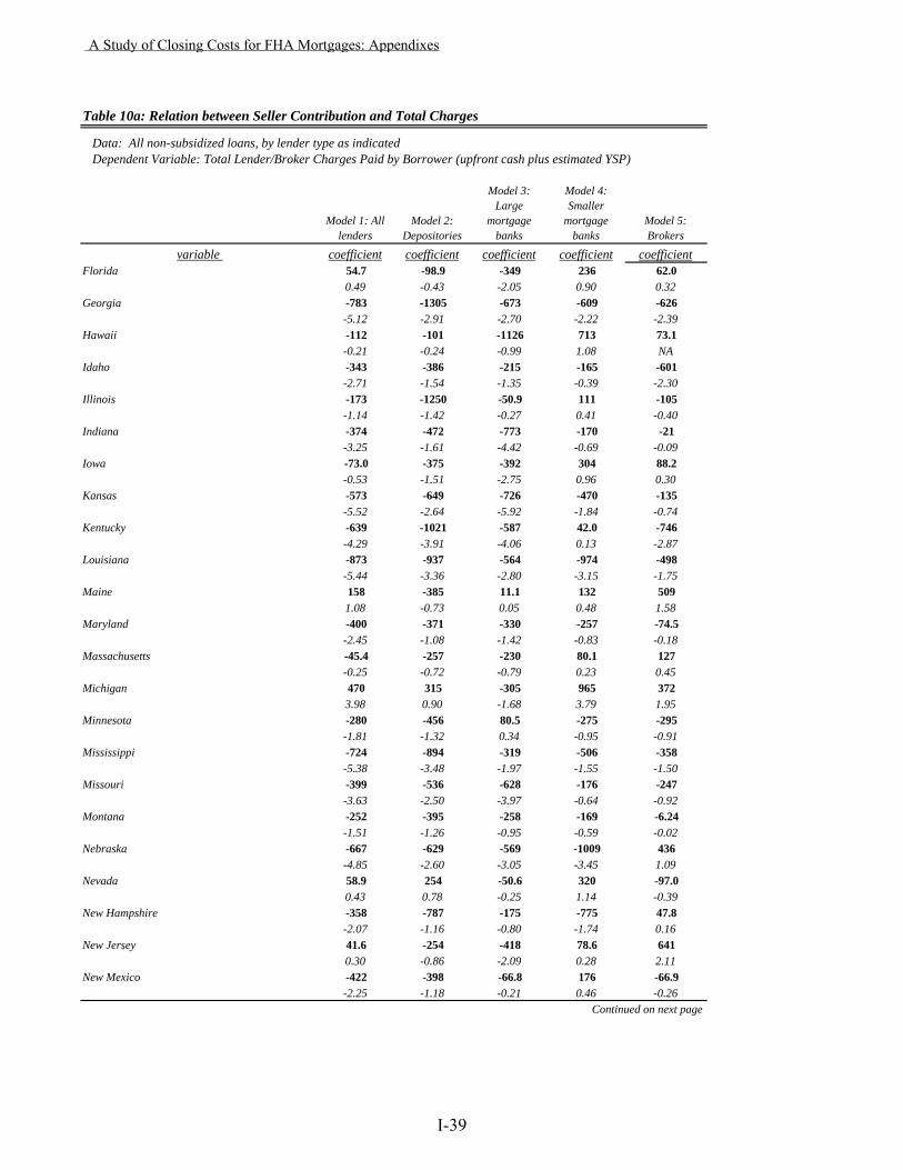
Table 10a: Relation between Seller Contribution and Total Charges
Data: All non-subsidized loans, by lender type as indicated Dependent Variable: Total Lender/Broker Charges Paid by Borrower (upfront cash plus estimated YSP)
Model 1: All lenders
Model 2: Depositories
Model 3: Large
mortgage banks
Model 4: Smaller
mortgage banks
Model 5: Brokers
variable coefficient coefficient coefficient coefficient coefficientFlorida 54.7 -98.9 -349 236 62.0
0.49 -0.43 -2.05 0.90 0.32Georgia -783 -1305 -673 -609 -626
-5.12 -2.91 -2.70 -2.22 -2.39Hawaii -112 -101 -1126 713 73.1
-0.21 -0.24 -0.99 1.08 NAIdaho -343 -386 -215 -165 -601
-2.71 -1.54 -1.35 -0.39 -2.30Illinois -173 -1250 -50.9 111 -105
-1.14 -1.42 -0.27 0.41 -0.40Indiana -374 -472 -773 -170 -21
-3.25 -1.61 -4.42 -0.69 -0.09Iowa -73.0 -375 -392 304 88.2
-0.53 -1.51 -2.75 0.96 0.30Kansas -573 -649 -726 -470 -135
-5.52 -2.64 -5.92 -1.84 -0.74Kentucky -639 -1021 -587 42.0 -746
-4.29 -3.91 -4.06 0.13 -2.87Louisiana -873 -937 -564 -974 -498
-5.44 -3.36 -2.80 -3.15 -1.75Maine 158 -385 11.1 132 509
1.08 -0.73 0.05 0.48 1.58Maryland -400 -371 -330 -257 -74.5
-2.45 -1.08 -1.42 -0.83 -0.18Massachusetts -45.4 -257 -230 80.1 127
-0.25 -0.72 -0.79 0.23 0.45Michigan 470 315 -305 965 372
3.98 0.90 -1.68 3.79 1.95Minnesota -280 -456 80.5 -275 -295
-1.81 -1.32 0.34 -0.95 -0.91Mississippi -724 -894 -319 -506 -358
-5.38 -3.48 -1.97 -1.55 -1.50Missouri -399 -536 -628 -176 -247
-3.63 -2.50 -3.97 -0.64 -0.92Montana -252 -395 -258 -169 -6.24
-1.51 -1.26 -0.95 -0.59 -0.02Nebraska -667 -629 -569 -1009 436
-4.85 -2.60 -3.05 -3.45 1.09Nevada 58.9 254 -50.6 320 -97.0
0.43 0.78 -0.25 1.14 -0.39New Hampshire -358 -787 -175 -775 47.8
-2.07 -1.16 -0.80 -1.74 0.16New Jersey 41.6 -254 -418 78.6 641
0.30 -0.86 -2.09 0.28 2.11New Mexico -422 -398 -66.8 176 -66.9
-2.25 -1.18 -0.21 0.46 -0.26Continued on next page
A Study of Closing Costs for FHA Mortgages: Appendixes
I-39
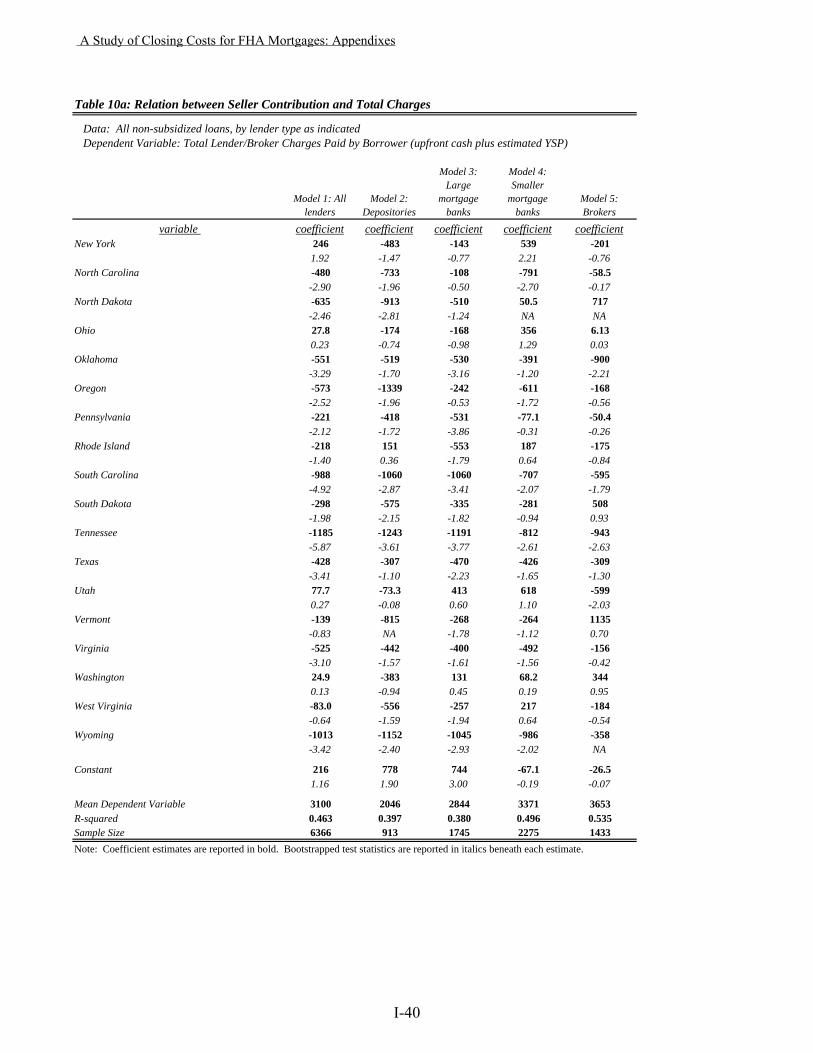
Table 10a: Relation between Seller Contribution and Total Charges
Data: All non-subsidized loans, by lender type as indicated Dependent Variable: Total Lender/Broker Charges Paid by Borrower (upfront cash plus estimated YSP)
Model 1: All lenders
Model 2: Depositories
Model 3: Large
mortgage banks
Model 4: Smaller
mortgage banks
Model 5: Brokers
variable coefficient coefficient coefficient coefficient coefficientNew York 246 -483 -143 539 -201
1.92 -1.47 -0.77 2.21 -0.76North Carolina -480 -733 -108 -791 -58.5
-2.90 -1.96 -0.50 -2.70 -0.17North Dakota -635 -913 -510 50.5 717
-2.46 -2.81 -1.24 NA NAOhio 27.8 -174 -168 356 6.13
0.23 -0.74 -0.98 1.29 0.03Oklahoma -551 -519 -530 -391 -900
-3.29 -1.70 -3.16 -1.20 -2.21Oregon -573 -1339 -242 -611 -168
-2.52 -1.96 -0.53 -1.72 -0.56Pennsylvania -221 -418 -531 -77.1 -50.4
-2.12 -1.72 -3.86 -0.31 -0.26Rhode Island -218 151 -553 187 -175
-1.40 0.36 -1.79 0.64 -0.84South Carolina -988 -1060 -1060 -707 -595
-4.92 -2.87 -3.41 -2.07 -1.79South Dakota -298 -575 -335 -281 508
-1.98 -2.15 -1.82 -0.94 0.93Tennessee -1185 -1243 -1191 -812 -943
-5.87 -3.61 -3.77 -2.61 -2.63Texas -428 -307 -470 -426 -309
-3.41 -1.10 -2.23 -1.65 -1.30Utah 77.7 -73.3 413 618 -599
0.27 -0.08 0.60 1.10 -2.03Vermont -139 -815 -268 -264 1135
-0.83 NA -1.78 -1.12 0.70Virginia -525 -442 -400 -492 -156
-3.10 -1.57 -1.61 -1.56 -0.42Washington 24.9 -383 131 68.2 344
0.13 -0.94 0.45 0.19 0.95West Virginia -83.0 -556 -257 217 -184
-0.64 -1.59 -1.94 0.64 -0.54Wyoming -1013 -1152 -1045 -986 -358
-3.42 -2.40 -2.93 -2.02 NA
Constant 216 778 744 -67.1 -26.51.16 1.90 3.00 -0.19 -0.07
Mean Dependent Variable 3100 2046 2844 3371 3653R-squared 0.463 0.397 0.380 0.496 0.535Sample Size 6366 913 1745 2275 1433Note: Coefficient estimates are reported in bold. Bootstrapped test statistics are reported in italics beneath each estimate.
A Study of Closing Costs for FHA Mortgages: Appendixes
I-40
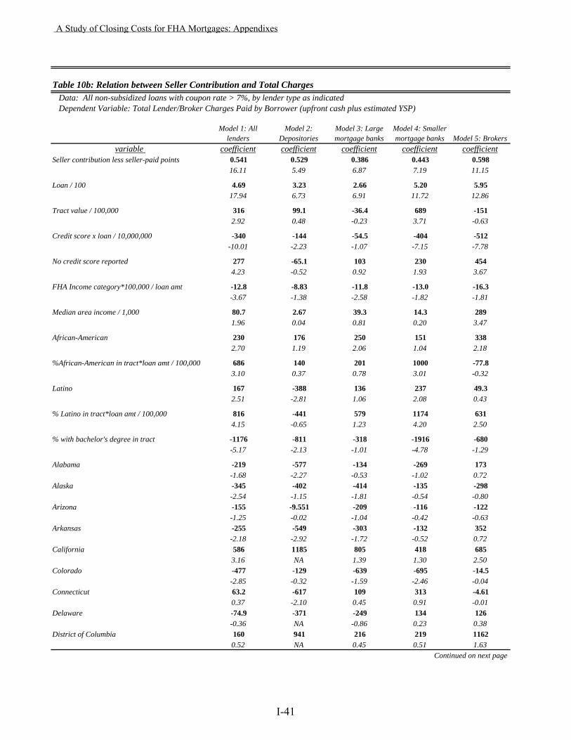
Table 10b: Relation between Seller Contribution and Total Charges Data: All non-subsidized loans with coupon rate > 7%, by lender type as indicated Dependent Variable: Total Lender/Broker Charges Paid by Borrower (upfront cash plus estimated YSP)
Model 1: All lenders
Model 2: Depositories
Model 3: Large mortgage banks
Model 4: Smaller mortgage banks Model 5: Brokers
variable coefficient coefficient coefficient coefficient coefficientSeller contribution less seller-paid points 0.541 0.529 0.386 0.443 0.598
16.11 5.49 6.87 7.19 11.15
Loan / 100 4.69 3.23 2.66 5.20 5.9517.94 6.73 6.91 11.72 12.86
Tract value / 100,000 316 99.1 -36.4 689 -1512.92 0.48 -0.23 3.71 -0.63
Credit score x loan / 10,000,000 -340 -144 -54.5 -404 -512-10.01 -2.23 -1.07 -7.15 -7.78
No credit score reported 277 -65.1 103 230 4544.23 -0.52 0.92 1.93 3.67
FHA Income category*100,000 / loan amt -12.8 -8.83 -11.8 -13.0 -16.3-3.67 -1.38 -2.58 -1.82 -1.81
Median area income / 1,000 80.7 2.67 39.3 14.3 2891.96 0.04 0.81 0.20 3.47
African-American 230 176 250 151 3382.70 1.19 2.06 1.04 2.18
%African-American in tract*loan amt / 100,000 686 140 201 1000 -77.83.10 0.37 0.78 3.01 -0.32
Latino 167 -388 136 237 49.32.51 -2.81 1.06 2.08 0.43
% Latino in tract*loan amt / 100,000 816 -441 579 1174 6314.15 -0.65 1.23 4.20 2.50
% with bachelor's degree in tract -1176 -811 -318 -1916 -680-5.17 -2.13 -1.01 -4.78 -1.29
Alabama -219 -577 -134 -269 173-1.68 -2.27 -0.53 -1.02 0.72
Alaska -345 -402 -414 -135 -298-2.54 -1.15 -1.81 -0.54 -0.80
Arizona -155 -9.551 -209 -116 -122-1.25 -0.02 -1.04 -0.42 -0.63
Arkansas -255 -549 -303 -132 352-2.18 -2.92 -1.72 -0.52 0.72
California 586 1185 805 418 6853.16 NA 1.39 1.30 2.50
Colorado -477 -129 -639 -695 -14.5-2.85 -0.32 -1.59 -2.46 -0.04
Connecticut 63.2 -617 109 313 -4.610.37 -2.10 0.45 0.91 -0.01
Delaware -74.9 -371 -249 134 126-0.36 NA -0.86 0.23 0.38
District of Columbia 160 941 216 219 11620.52 NA 0.45 0.51 1.63
Continued on next page
A Study of Closing Costs for FHA Mortgages: Appendixes
I-41
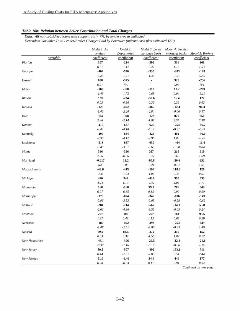
Table 10b: Relation between Seller Contribution and Total Charges Data: All non-subsidized loans with coupon rate > 7%, by lender type as indicated Dependent Variable: Total Lender/Broker Charges Paid by Borrower (upfront cash plus estimated YSP)
Model 1: All lenders
Model 2: Depositories
Model 3: Large mortgage banks
Model 4: Smaller mortgage banks Model 5: Brokers
variable coefficient coefficient coefficient coefficient coefficientFlorida 107 -224 -392 316 261
0.91 -1.17 -2.47 1.15 1.53Georgia -404 -550 -330 -383 -128
-3.25 -1.51 -1.30 -1.51 -0.55Hawaii 658 -575 - 920 -236
0.91 NA - 0.99 NAIdaho -169 -358 -113 13.2 -269
-1.43 -1.73 -0.68 0.04 -1.19Illinois 2.99 -234 -59.6 96.4 127
0.03 -0.36 -0.36 0.36 0.62Indiana -129 -402 -365 -12.4 96.3
-1.40 -2.20 -2.84 -0.06 0.47Iowa 304 -398 -128 920 650
2.46 -2.14 -1.03 2.55 2.58Kansas -415 -687 -625 -254 -86.7
-4.44 -4.18 -5.14 -0.91 -0.47Kentucky -290 -884 -429 402 -96.0
-2.30 -4.12 -2.96 1.05 -0.43Louisiana -513 -867 -650 -464 11.4
-3.49 -3.31 -3.65 -1.70 0.04Maine 346 -356 267 216 519
2.96 -0.86 1.95 0.66 1.68Maryland -0.617 18.2 -60.8 -20.6 652
NA 0.05 -0.24 -0.07 1.61Massachusetts -49.6 -415 -196 118.3 126
-0.36 -1.24 -1.06 0.36 0.51Michigan 470 344 -412 995 335
4.24 1.10 -2.42 4.03 1.71Minnesota 160 -168 99.3 280 349
0.97 -0.65 0.33 0.99 0.90Mississippi -376 -694 -345 -106 -149
-2.96 -3.53 -2.03 -0.28 -0.62Missouri -284 -714 -567 -14.3 55.8
-2.66 -4.36 -3.53 -0.05 0.24Montana 277 100 267 184 93.5
1.97 0.43 1.12 0.68 0.29Nebraska -180 -492 -398 -253 649
-1.47 -2.51 -2.09 -0.83 1.49Nevada 69.0 88.5 -272 319 152
0.53 0.32 -1.58 1.07 0.72New Hampshire -46.1 -306 -29.5 -22.4 -21.6
-0.38 -1.16 -0.19 -0.06 -0.08New Jersey 69.2 -507 -492 153.1 711
0.44 -2.31 -2.05 0.51 2.44New Mexico 51.0 -9.46 34.0 446 177
0.28 -0.03 0.11 0.91 0.64Continued on next page
A Study of Closing Costs for FHA Mortgages: Appendixes
I-42
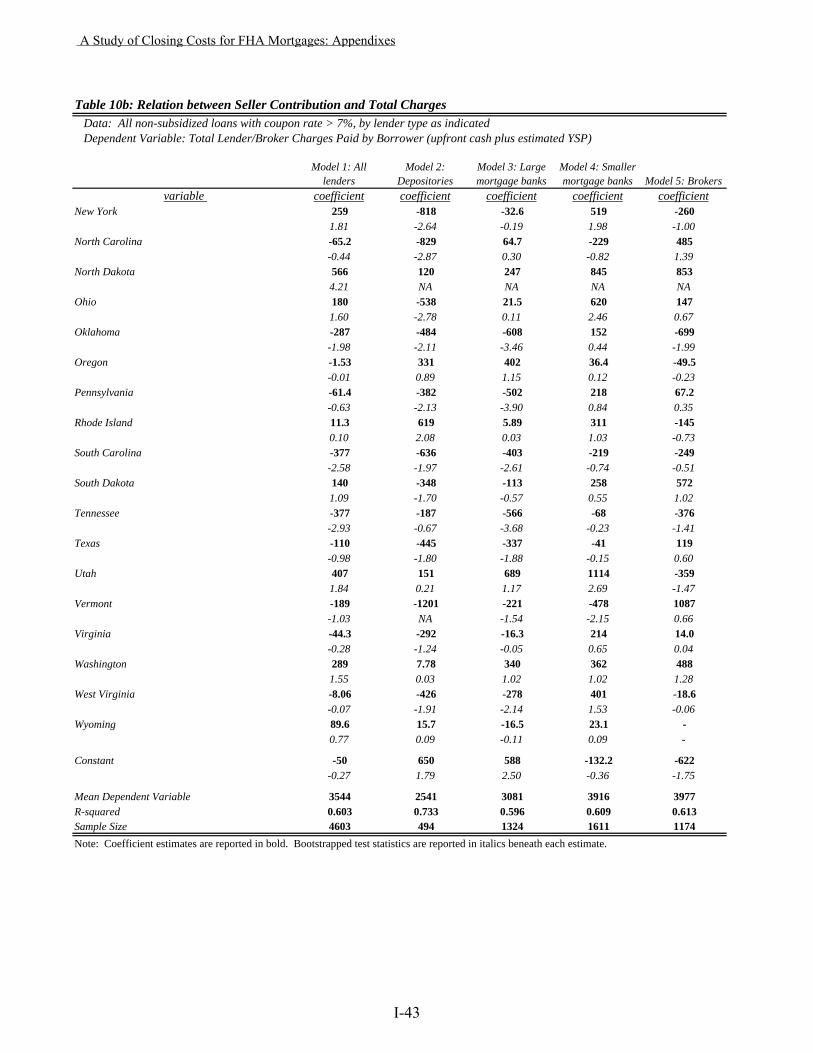
Table 10b: Relation between Seller Contribution and Total Charges Data: All non-subsidized loans with coupon rate > 7%, by lender type as indicated Dependent Variable: Total Lender/Broker Charges Paid by Borrower (upfront cash plus estimated YSP)
Model 1: All lenders
Model 2: Depositories
Model 3: Large mortgage banks
Model 4: Smaller mortgage banks Model 5: Brokers
variable coefficient coefficient coefficient coefficient coefficientNew York 259 -818 -32.6 519 -260
1.81 -2.64 -0.19 1.98 -1.00North Carolina -65.2 -829 64.7 -229 485
-0.44 -2.87 0.30 -0.82 1.39North Dakota 566 120 247 845 853
4.21 NA NA NA NAOhio 180 -538 21.5 620 147
1.60 -2.78 0.11 2.46 0.67Oklahoma -287 -484 -608 152 -699
-1.98 -2.11 -3.46 0.44 -1.99Oregon -1.53 331 402 36.4 -49.5
-0.01 0.89 1.15 0.12 -0.23Pennsylvania -61.4 -382 -502 218 67.2
-0.63 -2.13 -3.90 0.84 0.35Rhode Island 11.3 619 5.89 311 -145
0.10 2.08 0.03 1.03 -0.73South Carolina -377 -636 -403 -219 -249
-2.58 -1.97 -2.61 -0.74 -0.51South Dakota 140 -348 -113 258 572
1.09 -1.70 -0.57 0.55 1.02Tennessee -377 -187 -566 -68 -376
-2.93 -0.67 -3.68 -0.23 -1.41Texas -110 -445 -337 -41 119
-0.98 -1.80 -1.88 -0.15 0.60Utah 407 151 689 1114 -359
1.84 0.21 1.17 2.69 -1.47Vermont -189 -1201 -221 -478 1087
-1.03 NA -1.54 -2.15 0.66Virginia -44.3 -292 -16.3 214 14.0
-0.28 -1.24 -0.05 0.65 0.04Washington 289 7.78 340 362 488
1.55 0.03 1.02 1.02 1.28West Virginia -8.06 -426 -278 401 -18.6
-0.07 -1.91 -2.14 1.53 -0.06Wyoming 89.6 15.7 -16.5 23.1 -
0.77 0.09 -0.11 0.09 -
Constant -50 650 588 -132.2 -622-0.27 1.79 2.50 -0.36 -1.75
Mean Dependent Variable 3544 2541 3081 3916 3977R-squared 0.603 0.733 0.596 0.609 0.613Sample Size 4603 494 1324 1611 1174Note: Coefficient estimates are reported in bold. Bootstrapped test statistics are reported in italics beneath each estimate.
A Study of Closing Costs for FHA Mortgages: Appendixes
I-43
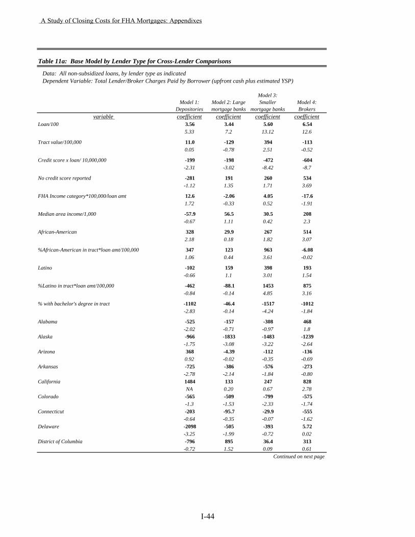
Table 11a: Base Model by Lender Type for Cross-Lender Comparisons
Data: All non-subsidized loans, by lender type as indicated Dependent Variable: Total Lender/Broker Charges Paid by Borrower (upfront cash plus estimated YSP)
Model 1: Depositories
Model 2: Large mortgage banks
Model 3: Smaller
mortgage banksModel 4: Brokers
variable coefficient coefficient coefficient coefficientLoan/100 3.56 3.44 5.60 6.54
5.33 7.2 13.12 12.6
Tract value/100,000 11.0 -129 394 -1130.05 -0.78 2.51 -0.52
Credit score x loan/ 10,000,000 -199 -198 -472 -604-2.31 -3.02 -8.42 -8.7
No credit score reported -281 191 260 534-1.12 1.35 1.71 3.69
FHA Income category*100,000/loan amt 12.6 -2.06 4.05 -17.61.72 -0.33 0.52 -1.91
Median area income/1,000 -57.9 56.5 30.5 208-0.67 1.11 0.42 2.3
African-American 328 29.9 267 5142.18 0.18 1.82 3.07
%African-American in tract*loan amt/100,000 347 123 963 -6.081.06 0.44 3.61 -0.02
Latino -102 159 398 193-0.66 1.1 3.01 1.54
%Latino in tract*loan amt/100,000 -462 -88.1 1453 875-0.84 -0.14 4.85 3.16
% with bachelor's degree in tract -1102 -46.4 -1517 -1012-2.83 -0.14 -4.24 -1.84
Alabama -525 -157 -308 468-2.02 -0.71 -0.97 1.8
Alaska -966 -1833 -1483 -1239-1.75 -3.08 -3.22 -2.64
Arizona 368 -4.39 -112 -1360.92 -0.02 -0.35 -0.69
Arkansas -725 -386 -576 -273-2.78 -2.14 -1.84 -0.80
California 1484 133 247 828NA 0.20 0.67 2.78
Colorado -565 -509 -799 -575-1.3 -1.53 -2.33 -1.74
Connecticut -203 -95.7 -29.9 -555-0.64 -0.35 -0.07 -1.62
Delaware -2098 -505 -393 5.72-3.25 -1.99 -0.72 0.02
District of Columbia -796 895 36.4 313-0.72 1.52 0.09 0.61
Continued on next page
A Study of Closing Costs for FHA Mortgages: Appendixes
I-44
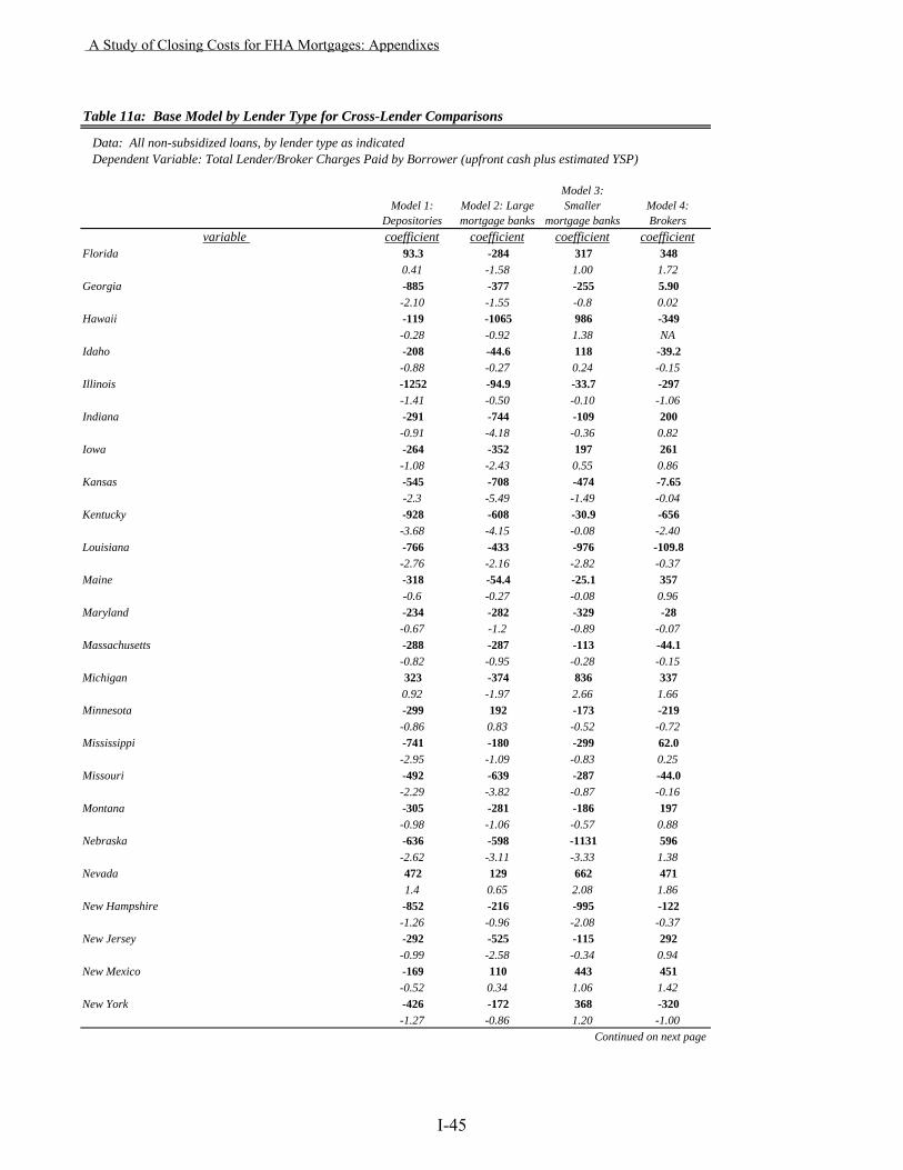
Table 11a: Base Model by Lender Type for Cross-Lender Comparisons
Data: All non-subsidized loans, by lender type as indicated Dependent Variable: Total Lender/Broker Charges Paid by Borrower (upfront cash plus estimated YSP)
Model 1: Depositories
Model 2: Large mortgage banks
Model 3: Smaller
mortgage banksModel 4: Brokers
variable coefficient coefficient coefficient coefficientFlorida 93.3 -284 317 348
0.41 -1.58 1.00 1.72Georgia -885 -377 -255 5.90
-2.10 -1.55 -0.8 0.02Hawaii -119 -1065 986 -349
-0.28 -0.92 1.38 NAIdaho -208 -44.6 118 -39.2
-0.88 -0.27 0.24 -0.15Illinois -1252 -94.9 -33.7 -297
-1.41 -0.50 -0.10 -1.06Indiana -291 -744 -109 200
-0.91 -4.18 -0.36 0.82Iowa -264 -352 197 261
-1.08 -2.43 0.55 0.86Kansas -545 -708 -474 -7.65
-2.3 -5.49 -1.49 -0.04Kentucky -928 -608 -30.9 -656
-3.68 -4.15 -0.08 -2.40Louisiana -766 -433 -976 -109.8
-2.76 -2.16 -2.82 -0.37Maine -318 -54.4 -25.1 357
-0.6 -0.27 -0.08 0.96Maryland -234 -282 -329 -28
-0.67 -1.2 -0.89 -0.07Massachusetts -288 -287 -113 -44.1
-0.82 -0.95 -0.28 -0.15Michigan 323 -374 836 337
0.92 -1.97 2.66 1.66Minnesota -299 192 -173 -219
-0.86 0.83 -0.52 -0.72Mississippi -741 -180 -299 62.0
-2.95 -1.09 -0.83 0.25Missouri -492 -639 -287 -44.0
-2.29 -3.82 -0.87 -0.16Montana -305 -281 -186 197
-0.98 -1.06 -0.57 0.88Nebraska -636 -598 -1131 596
-2.62 -3.11 -3.33 1.38Nevada 472 129 662 471
1.4 0.65 2.08 1.86New Hampshire -852 -216 -995 -122
-1.26 -0.96 -2.08 -0.37New Jersey -292 -525 -115 292
-0.99 -2.58 -0.34 0.94New Mexico -169 110 443 451
-0.52 0.34 1.06 1.42New York -426 -172 368 -320
-1.27 -0.86 1.20 -1.00Continued on next page
A Study of Closing Costs for FHA Mortgages: Appendixes
I-45
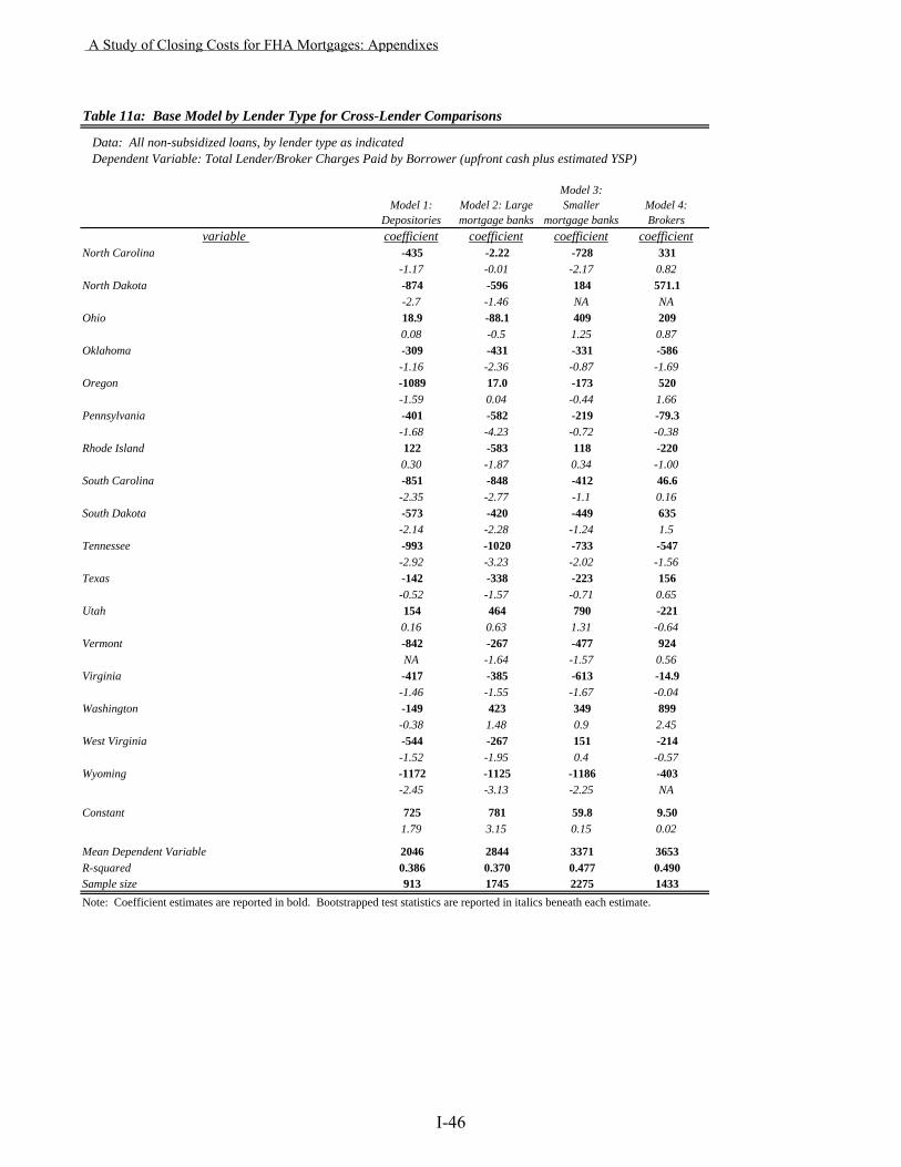
Table 11a: Base Model by Lender Type for Cross-Lender Comparisons
Data: All non-subsidized loans, by lender type as indicated Dependent Variable: Total Lender/Broker Charges Paid by Borrower (upfront cash plus estimated YSP)
Model 1: Depositories
Model 2: Large mortgage banks
Model 3: Smaller
mortgage banksModel 4: Brokers
variable coefficient coefficient coefficient coefficientNorth Carolina -435 -2.22 -728 331
-1.17 -0.01 -2.17 0.82North Dakota -874 -596 184 571.1
-2.7 -1.46 NA NAOhio 18.9 -88.1 409 209
0.08 -0.5 1.25 0.87Oklahoma -309 -431 -331 -586
-1.16 -2.36 -0.87 -1.69Oregon -1089 17.0 -173 520
-1.59 0.04 -0.44 1.66Pennsylvania -401 -582 -219 -79.3
-1.68 -4.23 -0.72 -0.38Rhode Island 122 -583 118 -220
0.30 -1.87 0.34 -1.00South Carolina -851 -848 -412 46.6
-2.35 -2.77 -1.1 0.16South Dakota -573 -420 -449 635
-2.14 -2.28 -1.24 1.5Tennessee -993 -1020 -733 -547
-2.92 -3.23 -2.02 -1.56Texas -142 -338 -223 156
-0.52 -1.57 -0.71 0.65Utah 154 464 790 -221
0.16 0.63 1.31 -0.64Vermont -842 -267 -477 924
NA -1.64 -1.57 0.56Virginia -417 -385 -613 -14.9
-1.46 -1.55 -1.67 -0.04Washington -149 423 349 899
-0.38 1.48 0.9 2.45West Virginia -544 -267 151 -214
-1.52 -1.95 0.4 -0.57Wyoming -1172 -1125 -1186 -403
-2.45 -3.13 -2.25 NA
Constant 725 781 59.8 9.501.79 3.15 0.15 0.02
Mean Dependent Variable 2046 2844 3371 3653R-squared 0.386 0.370 0.477 0.490Sample size 913 1745 2275 1433Note: Coefficient estimates are reported in bold. Bootstrapped test statistics are reported in italics beneath each estimate.
A Study of Closing Costs for FHA Mortgages: Appendixes
I-46
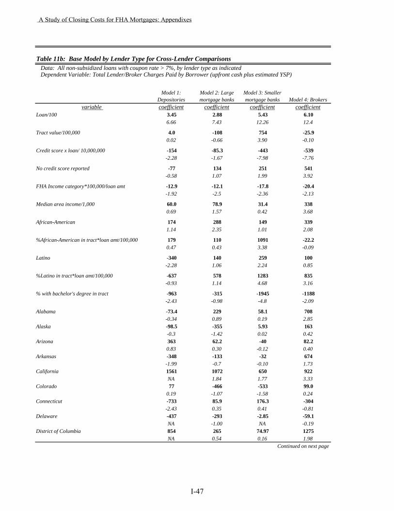
Table 11b: Base Model by Lender Type for Cross-Lender Comparisons Data: All non-subsidized loans with coupon rate > 7%, by lender type as indicated Dependent Variable: Total Lender/Broker Charges Paid by Borrower (upfront cash plus estimated YSP)
Model 1: Depositories
Model 2: Large mortgage banks
Model 3: Smaller mortgage banks Model 4: Brokers
variable coefficient coefficient coefficient coefficientLoan/100 3.45 2.88 5.43 6.10
6.66 7.43 12.26 12.4
Tract value/100,000 4.0 -108 754 -25.90.02 -0.66 3.90 -0.10
Credit score x loan/ 10,000,000 -154 -85.3 -443 -539-2.28 -1.67 -7.98 -7.76
No credit score reported -77 134 251 541-0.58 1.07 1.99 3.92
FHA Income category*100,000/loan amt -12.9 -12.1 -17.8 -20.4-1.92 -2.5 -2.36 -2.13
Median area income/1,000 60.0 78.9 31.4 3380.69 1.57 0.42 3.68
African-American 174 288 149 3391.14 2.35 1.01 2.08
%African-American in tract*loan amt/100,000 179 110 1091 -22.20.47 0.43 3.38 -0.09
Latino -340 140 259 100-2.28 1.06 2.24 0.85
%Latino in tract*loan amt/100,000 -637 578 1283 835-0.93 1.14 4.68 3.16
% with bachelor's degree in tract -963 -315 -1945 -1188-2.43 -0.98 -4.8 -2.09
Alabama -73.4 229 58.1 708-0.34 0.89 0.19 2.85
Alaska -98.5 -355 5.93 163-0.3 -1.42 0.02 0.42
Arizona 363 62.2 -40 82.20.83 0.30 -0.12 0.40
Arkansas -348 -133 -32 674-1.99 -0.7 -0.10 1.73
California 1561 1072 650 922NA 1.84 1.77 3.33
Colorado 77 -466 -533 99.00.19 -1.07 -1.58 0.24
Connecticut -733 85.9 176.3 -304-2.43 0.35 0.41 -0.81
Delaware -437 -293 -2.85 -59.1NA -1.00 NA -0.19
District of Columbia 854 265 74.97 1275NA 0.54 0.16 1.98
Continued on next page
A Study of Closing Costs for FHA Mortgages: Appendixes
I-47
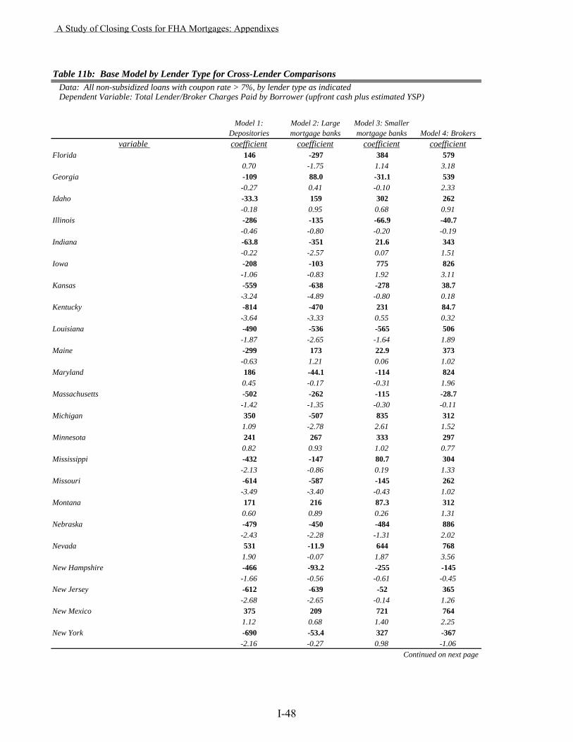
Table 11b: Base Model by Lender Type for Cross-Lender Comparisons Data: All non-subsidized loans with coupon rate > 7%, by lender type as indicated Dependent Variable: Total Lender/Broker Charges Paid by Borrower (upfront cash plus estimated YSP)
Model 1: Depositories
Model 2: Large mortgage banks
Model 3: Smaller mortgage banks Model 4: Brokers
variable coefficient coefficient coefficient coefficientFlorida 146 -297 384 579
0.70 -1.75 1.14 3.18Georgia -109 88.0 -31.1 539
-0.27 0.41 -0.10 2.33Idaho -33.3 159 302 262
-0.18 0.95 0.68 0.91Illinois -286 -135 -66.9 -40.7
-0.46 -0.80 -0.20 -0.19Indiana -63.8 -351 21.6 343
-0.22 -2.57 0.07 1.51Iowa -208 -103 775 826
-1.06 -0.83 1.92 3.11Kansas -559 -638 -278 38.7
-3.24 -4.89 -0.80 0.18Kentucky -814 -470 231 84.7
-3.64 -3.33 0.55 0.32Louisiana -490 -536 -565 506
-1.87 -2.65 -1.64 1.89Maine -299 173 22.9 373
-0.63 1.21 0.06 1.02Maryland 186 -44.1 -114 824
0.45 -0.17 -0.31 1.96Massachusetts -502 -262 -115 -28.7
-1.42 -1.35 -0.30 -0.11Michigan 350 -507 835 312
1.09 -2.78 2.61 1.52Minnesota 241 267 333 297
0.82 0.93 1.02 0.77Mississippi -432 -147 80.7 304
-2.13 -0.86 0.19 1.33Missouri -614 -587 -145 262
-3.49 -3.40 -0.43 1.02Montana 171 216 87.3 312
0.60 0.89 0.26 1.31Nebraska -479 -450 -484 886
-2.43 -2.28 -1.31 2.02Nevada 531 -11.9 644 768
1.90 -0.07 1.87 3.56New Hampshire -466 -93.2 -255 -145
-1.66 -0.56 -0.61 -0.45New Jersey -612 -639 -52 365
-2.68 -2.65 -0.14 1.26New Mexico 375 209 721 764
1.12 0.68 1.40 2.25New York -690 -53.4 327 -367
-2.16 -0.27 0.98 -1.06Continued on next page
A Study of Closing Costs for FHA Mortgages: Appendixes
I-48
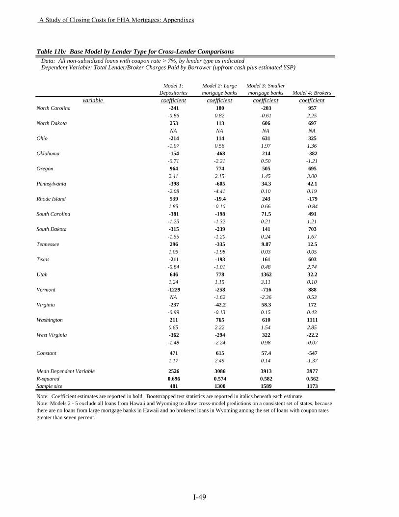
Table 11b: Base Model by Lender Type for Cross-Lender Comparisons Data: All non-subsidized loans with coupon rate > 7%, by lender type as indicated Dependent Variable: Total Lender/Broker Charges Paid by Borrower (upfront cash plus estimated YSP)
Model 1: Depositories
Model 2: Large mortgage banks
Model 3: Smaller mortgage banks Model 4: Brokers
variable coefficient coefficient coefficient coefficientNorth Carolina -241 180 -203 957
-0.86 0.82 -0.61 2.25North Dakota 253 113 606 697
NA NA NA NAOhio -214 114 631 325
-1.07 0.56 1.97 1.36Oklahoma -154 -468 214 -382
-0.71 -2.21 0.50 -1.21Oregon 964 774 505 695
2.41 2.15 1.45 3.00Pennsylvania -398 -605 34.3 42.1
-2.08 -4.41 0.10 0.19Rhode Island 539 -19.4 243 -179
1.85 -0.10 0.66 -0.84South Carolina -381 -198 71.5 491
-1.25 -1.32 0.21 1.21South Dakota -315 -239 141 703
-1.55 -1.20 0.24 1.67Tennessee 296 -335 9.87 12.5
1.05 -1.98 0.03 0.05Texas -211 -193 161 603
-0.84 -1.01 0.48 2.74Utah 646 778 1362 32.2
1.24 1.15 3.11 0.10Vermont -1229 -258 -716 888
NA -1.62 -2.36 0.53Virginia -237 -42.2 58.3 172
-0.99 -0.13 0.15 0.43Washington 211 765 610 1111
0.65 2.22 1.54 2.85West Virginia -362 -294 322 -22.2
-1.48 -2.24 0.98 -0.07
Constant 471 615 57.4 -5471.17 2.49 0.14 -1.37
Mean Dependent Variable 2526 3086 3913 3977R-squared 0.696 0.574 0.582 0.562Sample size 481 1300 1589 1173
Note: Coefficient estimates are reported in bold. Bootstrapped test statistics are reported in italics beneath each estimate.Note: Models 2 - 5 exclude all loans from Hawaii and Wyoming to allow cross-model predictions on a consistent set of states, because there are no loans from large mortgage banks in Hawaii and no brokered loans in Wyoming among the set of loans with coupon rates greater than seven percent.
A Study of Closing Costs for FHA Mortgages: Appendixes
I-49
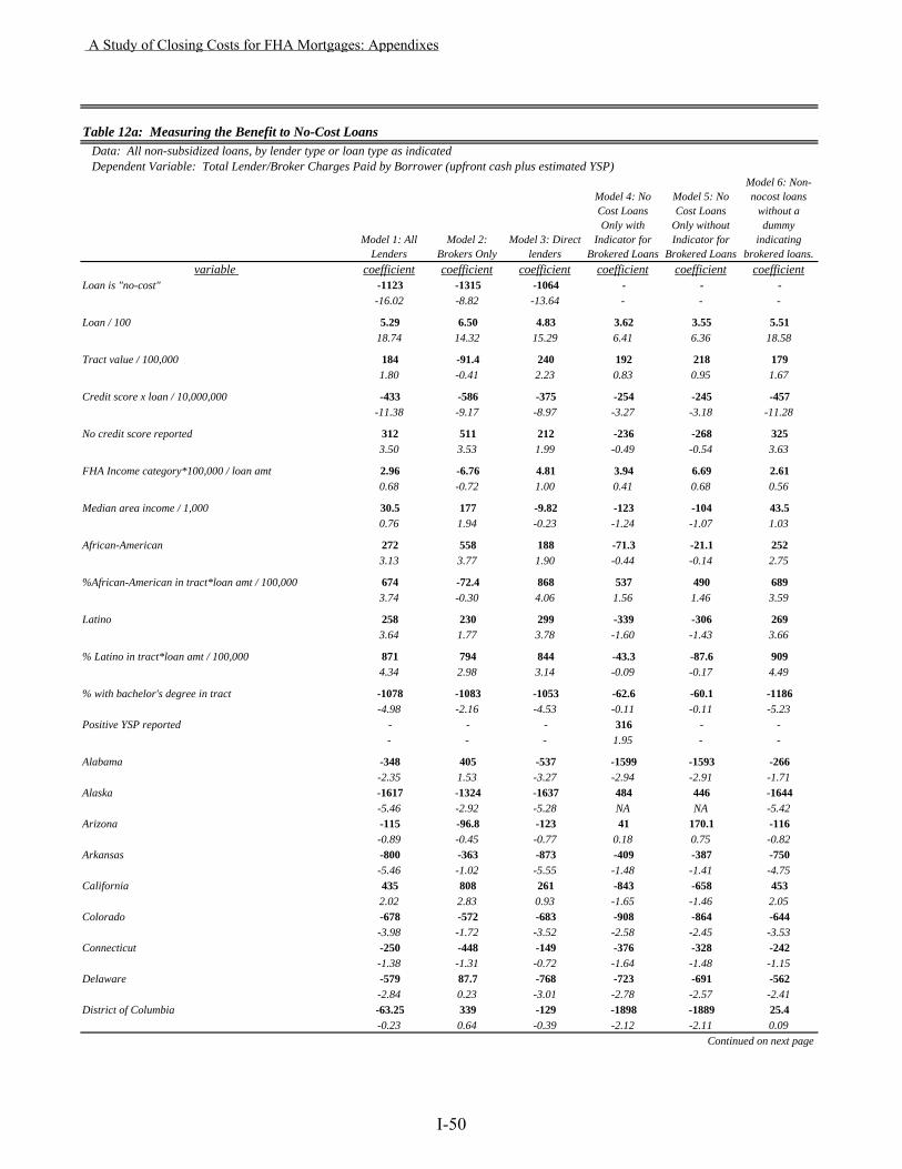
Table 12a: Measuring the Benefit to No-Cost Loans Data: All non-subsidized loans, by lender type or loan type as indicated Dependent Variable: Total Lender/Broker Charges Paid by Borrower (upfront cash plus estimated YSP)
Model 1: All Lenders
Model 2: Brokers Only
Model 3: Direct lenders
Model 4: No Cost Loans Only with
Indicator for Brokered Loans
Model 5: No Cost Loans
Only without Indicator for
Brokered Loans
Model 6: Non-nocost loans
without a dummy
indicating brokered loans.
variable coefficient coefficient coefficient coefficient coefficient coefficientLoan is "no-cost" -1123 -1315 -1064 - - -
-16.02 -8.82 -13.64 - - -
Loan / 100 5.29 6.50 4.83 3.62 3.55 5.5118.74 14.32 15.29 6.41 6.36 18.58
Tract value / 100,000 184 -91.4 240 192 218 1791.80 -0.41 2.23 0.83 0.95 1.67
Credit score x loan / 10,000,000 -433 -586 -375 -254 -245 -457-11.38 -9.17 -8.97 -3.27 -3.18 -11.28
No credit score reported 312 511 212 -236 -268 3253.50 3.53 1.99 -0.49 -0.54 3.63
FHA Income category*100,000 / loan amt 2.96 -6.76 4.81 3.94 6.69 2.610.68 -0.72 1.00 0.41 0.68 0.56
Median area income / 1,000 30.5 177 -9.82 -123 -104 43.50.76 1.94 -0.23 -1.24 -1.07 1.03
African-American 272 558 188 -71.3 -21.1 2523.13 3.77 1.90 -0.44 -0.14 2.75
%African-American in tract*loan amt / 100,000 674 -72.4 868 537 490 6893.74 -0.30 4.06 1.56 1.46 3.59
Latino 258 230 299 -339 -306 2693.64 1.77 3.78 -1.60 -1.43 3.66
% Latino in tract*loan amt / 100,000 871 794 844 -43.3 -87.6 9094.34 2.98 3.14 -0.09 -0.17 4.49
% with bachelor's degree in tract -1078 -1083 -1053 -62.6 -60.1 -1186-4.98 -2.16 -4.53 -0.11 -0.11 -5.23
Positive YSP reported - - - 316 - -- - - 1.95 - -
Alabama -348 405 -537 -1599 -1593 -266-2.35 1.53 -3.27 -2.94 -2.91 -1.71
Alaska -1617 -1324 -1637 484 446 -1644-5.46 -2.92 -5.28 NA NA -5.42
Arizona -115 -96.8 -123 41 170.1 -116-0.89 -0.45 -0.77 0.18 0.75 -0.82
Arkansas -800 -363 -873 -409 -387 -750-5.46 -1.02 -5.55 -1.48 -1.41 -4.75
California 435 808 261 -843 -658 4532.02 2.83 0.93 -1.65 -1.46 2.05
Colorado -678 -572 -683 -908 -864 -644-3.98 -1.72 -3.52 -2.58 -2.45 -3.53
Connecticut -250 -448 -149 -376 -328 -242-1.38 -1.31 -0.72 -1.64 -1.48 -1.15
Delaware -579 87.7 -768 -723 -691 -562-2.84 0.23 -3.01 -2.78 -2.57 -2.41
District of Columbia -63.25 339 -129 -1898 -1889 25.4-0.23 0.64 -0.39 -2.12 -2.11 0.09
Continued on next page
A Study of Closing Costs for FHA Mortgages: Appendixes
I-50
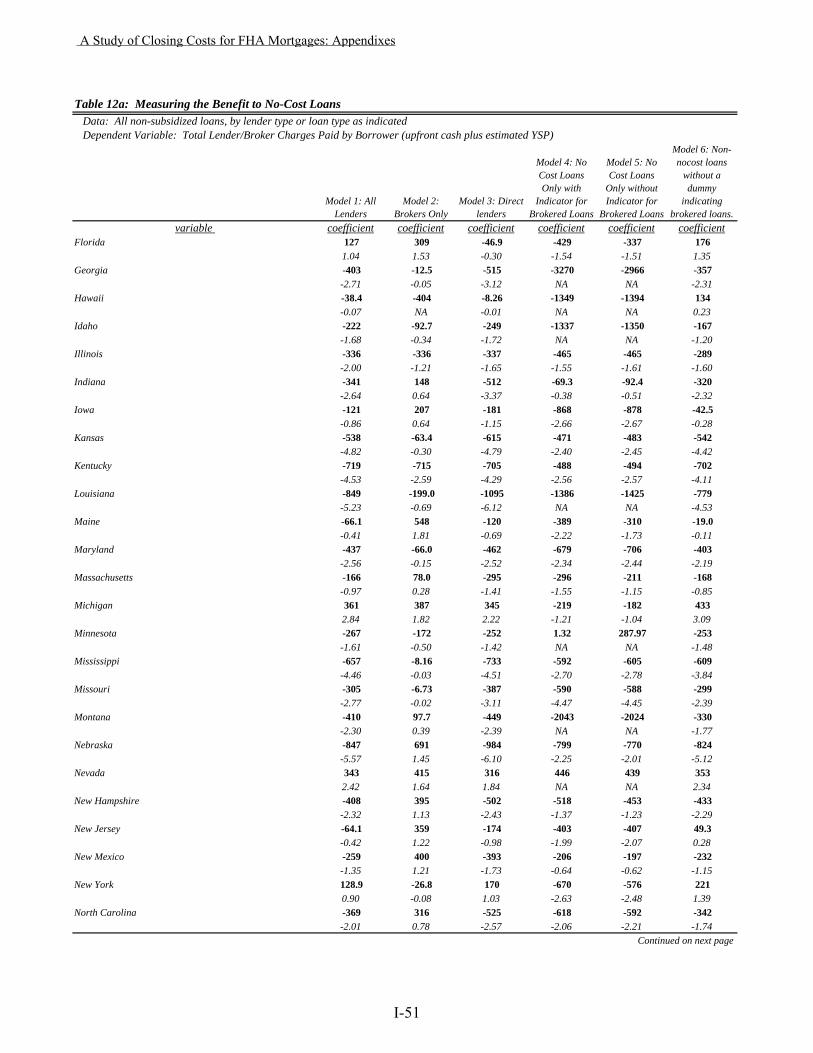
Table 12a: Measuring the Benefit to No-Cost Loans Data: All non-subsidized loans, by lender type or loan type as indicated Dependent Variable: Total Lender/Broker Charges Paid by Borrower (upfront cash plus estimated YSP)
Model 1: All Lenders
Model 2: Brokers Only
Model 3: Direct lenders
Model 4: No Cost Loans Only with
Indicator for Brokered Loans
Model 5: No Cost Loans
Only without Indicator for
Brokered Loans
Model 6: Non-nocost loans
without a dummy
indicating brokered loans.
variable coefficient coefficient coefficient coefficient coefficient coefficientFlorida 127 309 -46.9 -429 -337 176
1.04 1.53 -0.30 -1.54 -1.51 1.35Georgia -403 -12.5 -515 -3270 -2966 -357
-2.71 -0.05 -3.12 NA NA -2.31Hawaii -38.4 -404 -8.26 -1349 -1394 134
-0.07 NA -0.01 NA NA 0.23Idaho -222 -92.7 -249 -1337 -1350 -167
-1.68 -0.34 -1.72 NA NA -1.20Illinois -336 -336 -337 -465 -465 -289
-2.00 -1.21 -1.65 -1.55 -1.61 -1.60Indiana -341 148 -512 -69.3 -92.4 -320
-2.64 0.64 -3.37 -0.38 -0.51 -2.32Iowa -121 207 -181 -868 -878 -42.5
-0.86 0.64 -1.15 -2.66 -2.67 -0.28Kansas -538 -63.4 -615 -471 -483 -542
-4.82 -0.30 -4.79 -2.40 -2.45 -4.42Kentucky -719 -715 -705 -488 -494 -702
-4.53 -2.59 -4.29 -2.56 -2.57 -4.11Louisiana -849 -199.0 -1095 -1386 -1425 -779
-5.23 -0.69 -6.12 NA NA -4.53Maine -66.1 548 -120 -389 -310 -19.0
-0.41 1.81 -0.69 -2.22 -1.73 -0.11Maryland -437 -66.0 -462 -679 -706 -403
-2.56 -0.15 -2.52 -2.34 -2.44 -2.19Massachusetts -166 78.0 -295 -296 -211 -168
-0.97 0.28 -1.41 -1.55 -1.15 -0.85Michigan 361 387 345 -219 -182 433
2.84 1.82 2.22 -1.21 -1.04 3.09Minnesota -267 -172 -252 1.32 287.97 -253
-1.61 -0.50 -1.42 NA NA -1.48Mississippi -657 -8.16 -733 -592 -605 -609
-4.46 -0.03 -4.51 -2.70 -2.78 -3.84Missouri -305 -6.73 -387 -590 -588 -299
-2.77 -0.02 -3.11 -4.47 -4.45 -2.39Montana -410 97.7 -449 -2043 -2024 -330
-2.30 0.39 -2.39 NA NA -1.77Nebraska -847 691 -984 -799 -770 -824
-5.57 1.45 -6.10 -2.25 -2.01 -5.12Nevada 343 415 316 446 439 353
2.42 1.64 1.84 NA NA 2.34New Hampshire -408 395 -502 -518 -453 -433
-2.32 1.13 -2.43 -1.37 -1.23 -2.29New Jersey -64.1 359 -174 -403 -407 49.3
-0.42 1.22 -0.98 -1.99 -2.07 0.28New Mexico -259 400 -393 -206 -197 -232
-1.35 1.21 -1.73 -0.64 -0.62 -1.15New York 128.9 -26.8 170 -670 -576 221
0.90 -0.08 1.03 -2.63 -2.48 1.39North Carolina -369 316 -525 -618 -592 -342
-2.01 0.78 -2.57 -2.06 -2.21 -1.74Continued on next page
A Study of Closing Costs for FHA Mortgages: Appendixes
I-51
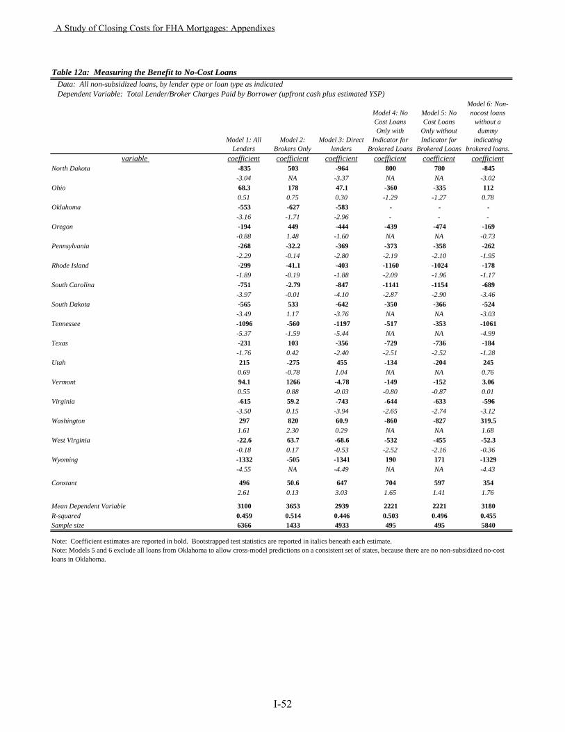
Table 12a: Measuring the Benefit to No-Cost Loans Data: All non-subsidized loans, by lender type or loan type as indicated Dependent Variable: Total Lender/Broker Charges Paid by Borrower (upfront cash plus estimated YSP)
Model 1: All Lenders
Model 2: Brokers Only
Model 3: Direct lenders
Model 4: No Cost Loans Only with
Indicator for Brokered Loans
Model 5: No Cost Loans
Only without Indicator for
Brokered Loans
Model 6: Non-nocost loans
without a dummy
indicating brokered loans.
variable coefficient coefficient coefficient coefficient coefficient coefficientNorth Dakota -835 503 -964 800 780 -845
-3.04 NA -3.37 NA NA -3.02Ohio 68.3 178 47.1 -360 -335 112
0.51 0.75 0.30 -1.29 -1.27 0.78Oklahoma -553 -627 -583 - - -
-3.16 -1.71 -2.96 - - -Oregon -194 449 -444 -439 -474 -169
-0.88 1.48 -1.60 NA NA -0.73Pennsylvania -268 -32.2 -369 -373 -358 -262
-2.29 -0.14 -2.80 -2.19 -2.10 -1.95Rhode Island -299 -41.1 -403 -1160 -1024 -178
-1.89 -0.19 -1.88 -2.09 -1.96 -1.17South Carolina -751 -2.79 -847 -1141 -1154 -689
-3.97 -0.01 -4.10 -2.87 -2.90 -3.46South Dakota -565 533 -642 -350 -366 -524
-3.49 1.17 -3.76 NA NA -3.03Tennessee -1096 -560 -1197 -517 -353 -1061
-5.37 -1.59 -5.44 NA NA -4.99Texas -231 103 -356 -729 -736 -184
-1.76 0.42 -2.40 -2.51 -2.52 -1.28Utah 215 -275 455 -134 -204 245
0.69 -0.78 1.04 NA NA 0.76Vermont 94.1 1266 -4.78 -149 -152 3.06
0.55 0.88 -0.03 -0.80 -0.87 0.01Virginia -615 59.2 -743 -644 -633 -596
-3.50 0.15 -3.94 -2.65 -2.74 -3.12Washington 297 820 60.9 -860 -827 319.5
1.61 2.30 0.29 NA NA 1.68West Virginia -22.6 63.7 -68.6 -532 -455 -52.3
-0.18 0.17 -0.53 -2.52 -2.16 -0.36Wyoming -1332 -505 -1341 190 171 -1329
-4.55 NA -4.49 NA NA -4.43
Constant 496 50.6 647 704 597 3542.61 0.13 3.03 1.65 1.41 1.76
Mean Dependent Variable 3100 3653 2939 2221 2221 3180R-squared 0.459 0.514 0.446 0.503 0.496 0.455Sample size 6366 1433 4933 495 495 5840
Note: Coefficient estimates are reported in bold. Bootstrapped test statistics are reported in italics beneath each estimate.Note: Models 5 and 6 exclude all loans from Oklahoma to allow cross-model predictions on a consistent set of states, because there are no non-subsidized no-cost loans in Oklahoma.
A Study of Closing Costs for FHA Mortgages: Appendixes
I-52

Table 12b: Measuring the Benefit to No-Cost Loans Data: All non-subsidized loans with coupon rate > 7%, by lender type or loan type as indicated Dependent Variable: Total Lender/Broker Charges Paid by Borrower (upfront cash plus estimated YSP)
Model 1: All Lenders
Model 2: Brokers Only
Model 3: Direct lenders
Model 4: Nocost loans with a dummy
indicating brokered loans
Model 5: Nocost loans
without a dummy
indicating brokered loans
Model 6: Non-nocost loans
without a dummy
indicating brokered
loans.variable coefficient coefficient coefficient coefficient coefficient coefficient
Loan is "no-cost" -1303 -1387 -1246 - - --28.16 -10.46 -23.94 - - -
Loan / 100 4.99 5.97 4.48 2.95 2.93 5.3821.64 12.80 16.60 8.05 8.01 21.06
Tract value / 100,000 347 12.7 438 96 100.8 3743.48 0.05 3.87 0.54 0.58 3.40
Credit score x loan / 10,000,000 -366 -506 -297 -134 -131 -414-11.68 -7.38 -8.55 -2.74 -2.68 -11.75
No credit score reported 319 515 218 99.0 91.0 3034.45 3.81 2.60 0.75 0.70 3.84
FHA Income category*100,000 / loan amt -11.1 -6.44 -11.6 -6.16 -5.43 -11.4-3.20 -0.70 -3.09 -1.15 -1.00 -2.95
Median area income / 1,000 58.3 293 5.90 -106 -100 84.51.46 3.35 0.13 -1.19 -1.15 1.95
African-American 238 389 178 -99.5 -85.5 1782.92 2.61 1.84 -0.84 -0.74 1.99
%African-American in tract*loan amt / 100,000 686 -90.9 930 406 392 8073.49 -0.36 4.13 1.33 1.29 3.69
Latino 193 136 231 -352 -345 1923.18 1.21 3.03 -2.10 -2.05 2.97
% Latino in tract*loan amt / 100,000 910 748 979 -325 -336 9824.79 2.78 3.78 -0.67 -0.70 5.43
% with bachelor's degree in tract -1225 -1274 -1192 -110 -105 -1392-5.45 -2.19 -5.23 -0.29 -0.28 -5.56
Positive YSP reported - - - 93.3 - -- - - 1.15 - -
Alabama 59.5 641 -142 -456 -455 1470.46 2.64 -1.00 NA NA 1.05
Alaska -282 63.5 -325 254 242 -309-2.05 0.16 -2.31 NA NA -2.05
Arizona -48.2 149 -118.6 193 232 -42.6-0.40 0.80 -0.74 0.93 1.12 -0.32
Arkansas -240 532 -351 -432 -427 -166-2.04 1.49 -2.74 -1.70 -1.68 -1.29
California 711 896 725 -586 -529 7264.47 3.35 3.58 -1.27 -1.18 4.45
Colorado -354 188 -470 -514 -495 -299-2.21 0.47 -2.63 -1.85 -1.81 -1.72
Connecticut -36.3 -90.0 -8.4 -167 -150 -18.5-0.21 -0.25 -0.04 -0.90 -0.83 -0.08
Continued on next page
A Study of Closing Costs for FHA Mortgages: Appendixes
I-53
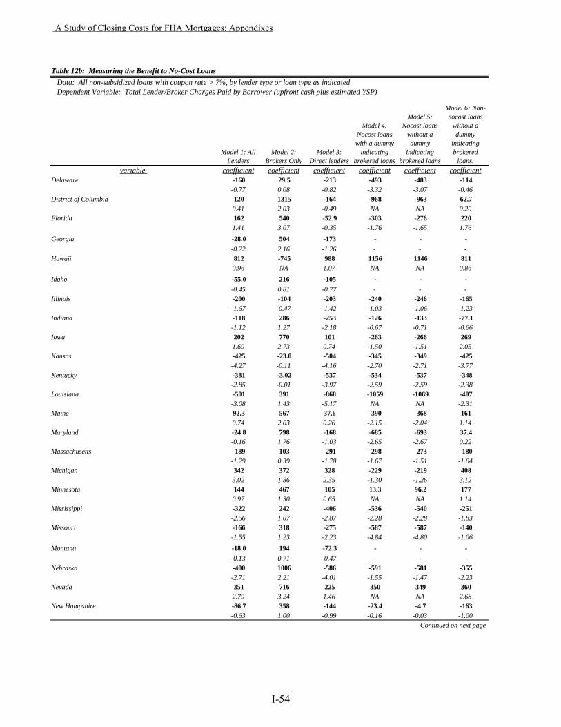
Table 12b: Measuring the Benefit to No-Cost Loans Data: All non-subsidized loans with coupon rate > 7%, by lender type or loan type as indicated Dependent Variable: Total Lender/Broker Charges Paid by Borrower (upfront cash plus estimated YSP)
Model 1: All Lenders
Model 2: Brokers Only
Model 3: Direct lenders
Model 4: Nocost loans with a dummy
indicating brokered loans
Model 5: Nocost loans
without a dummy
indicating brokered loans
Model 6: Non-nocost loans
without a dummy
indicating brokered
loans.variable coefficient coefficient coefficient coefficient coefficient coefficient
Delaware -160 29.5 -213 -493 -483 -114-0.77 0.08 -0.82 -3.32 -3.07 -0.46
District of Columbia 120 1315 -164 -968 -963 62.70.41 2.03 -0.49 NA NA 0.20
Florida 162 540 -52.9 -303 -276 2201.41 3.07 -0.35 -1.76 -1.65 1.76
Georgia -28.0 504 -173 - - --0.22 2.16 -1.26 - - -
Hawaii 812 -745 988 1156 1146 8110.96 NA 1.07 NA NA 0.86
Idaho -55.0 216 -105 - - --0.45 0.81 -0.77 - - -
Illinois -200 -104 -203 -240 -246 -165-1.67 -0.47 -1.42 -1.03 -1.06 -1.23
Indiana -118 286 -253 -126 -133 -77.1-1.12 1.27 -2.18 -0.67 -0.71 -0.66
Iowa 202 770 101 -263 -266 2691.69 2.73 0.74 -1.50 -1.51 2.05
Kansas -425 -23.0 -504 -345 -349 -425-4.27 -0.11 -4.16 -2.70 -2.71 -3.77
Kentucky -381 -3.02 -537 -534 -537 -348-2.85 -0.01 -3.97 -2.59 -2.59 -2.38
Louisiana -501 391 -868 -1059 -1069 -407-3.08 1.43 -5.17 NA NA -2.31
Maine 92.3 567 37.6 -390 -368 1610.74 2.03 0.26 -2.15 -2.04 1.14
Maryland -24.8 798 -168 -685 -693 37.4-0.16 1.76 -1.03 -2.65 -2.67 0.22
Massachusetts -189 103 -291 -298 -273 -180-1.29 0.39 -1.78 -1.67 -1.51 -1.04
Michigan 342 372 328 -229 -219 4083.02 1.86 2.35 -1.30 -1.26 3.12
Minnesota 144 467 105 13.3 96.2 1770.97 1.30 0.65 NA NA 1.14
Mississippi -322 242 -406 -536 -540 -251-2.56 1.07 -2.87 -2.28 -2.28 -1.83
Missouri -166 318 -275 -587 -587 -140-1.55 1.23 -2.23 -4.84 -4.80 -1.06
Montana -18.0 194 -72.3 - - --0.13 0.71 -0.47 - - -
Nebraska -400 1006 -586 -591 -581 -355-2.71 2.21 -4.01 -1.55 -1.47 -2.23
Nevada 351 716 225 350 349 3602.79 3.24 1.46 NA NA 2.68
New Hampshire -86.7 358 -144 -23.4 -4.7 -163-0.63 1.00 -0.99 -0.16 -0.03 -1.00
Continued on next page
A Study of Closing Costs for FHA Mortgages: Appendixes
I-54
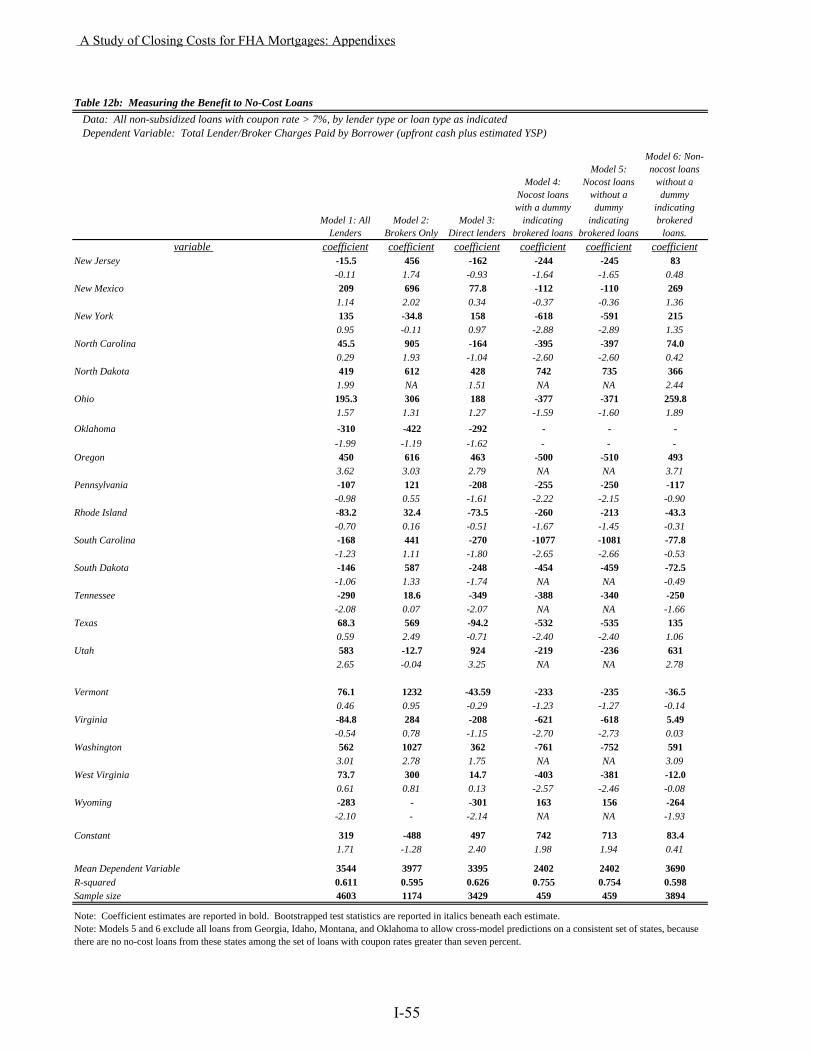
Table 12b: Measuring the Benefit to No-Cost Loans Data: All non-subsidized loans with coupon rate > 7%, by lender type or loan type as indicated Dependent Variable: Total Lender/Broker Charges Paid by Borrower (upfront cash plus estimated YSP)
Model 1: All Lenders
Model 2: Brokers Only
Model 3: Direct lenders
Model 4: Nocost loans with a dummy
indicating brokered loans
Model 5: Nocost loans
without a dummy
indicating brokered loans
Model 6: Non-nocost loans
without a dummy
indicating brokered
loans.variable coefficient coefficient coefficient coefficient coefficient coefficient
New Jersey -15.5 456 -162 -244 -245 83-0.11 1.74 -0.93 -1.64 -1.65 0.48
New Mexico 209 696 77.8 -112 -110 2691.14 2.02 0.34 -0.37 -0.36 1.36
New York 135 -34.8 158 -618 -591 2150.95 -0.11 0.97 -2.88 -2.89 1.35
North Carolina 45.5 905 -164 -395 -397 74.00.29 1.93 -1.04 -2.60 -2.60 0.42
North Dakota 419 612 428 742 735 3661.99 NA 1.51 NA NA 2.44
Ohio 195.3 306 188 -377 -371 259.81.57 1.31 1.27 -1.59 -1.60 1.89
Oklahoma -310 -422 -292 - - --1.99 -1.19 -1.62 - - -
Oregon 450 616 463 -500 -510 4933.62 3.03 2.79 NA NA 3.71
Pennsylvania -107 121 -208 -255 -250 -117-0.98 0.55 -1.61 -2.22 -2.15 -0.90
Rhode Island -83.2 32.4 -73.5 -260 -213 -43.3-0.70 0.16 -0.51 -1.67 -1.45 -0.31
South Carolina -168 441 -270 -1077 -1081 -77.8-1.23 1.11 -1.80 -2.65 -2.66 -0.53
South Dakota -146 587 -248 -454 -459 -72.5-1.06 1.33 -1.74 NA NA -0.49
Tennessee -290 18.6 -349 -388 -340 -250-2.08 0.07 -2.07 NA NA -1.66
Texas 68.3 569 -94.2 -532 -535 1350.59 2.49 -0.71 -2.40 -2.40 1.06
Utah 583 -12.7 924 -219 -236 6312.65 -0.04 3.25 NA NA 2.78
Vermont 76.1 1232 -43.59 -233 -235 -36.50.46 0.95 -0.29 -1.23 -1.27 -0.14
Virginia -84.8 284 -208 -621 -618 5.49-0.54 0.78 -1.15 -2.70 -2.73 0.03
Washington 562 1027 362 -761 -752 5913.01 2.78 1.75 NA NA 3.09
West Virginia 73.7 300 14.7 -403 -381 -12.00.61 0.81 0.13 -2.57 -2.46 -0.08
Wyoming -283 - -301 163 156 -264-2.10 - -2.14 NA NA -1.93
Constant 319 -488 497 742 713 83.41.71 -1.28 2.40 1.98 1.94 0.41
Mean Dependent Variable 3544 3977 3395 2402 2402 3690R-squared 0.611 0.595 0.626 0.755 0.754 0.598Sample size 4603 1174 3429 459 459 3894
Note: Coefficient estimates are reported in bold. Bootstrapped test statistics are reported in italics beneath each estimate.Note: Models 5 and 6 exclude all loans from Georgia, Idaho, Montana, and Oklahoma to allow cross-model predictions on a consistent set of states, because there are no no-cost loans from these states among the set of loans with coupon rates greater than seven percent.
A Study of Closing Costs for FHA Mortgages: Appendixes
I-55
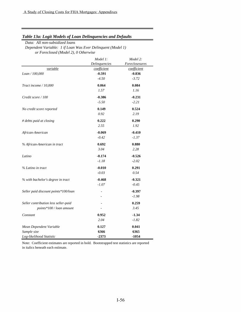
Data: All non-subsidized loans Dependent Variable: 1 if Loan Was Ever Delinquent (Model 1) or Foreclosed (Model 2), 0 Otherwise
Model 1: Delinquencies
Model 2: Foreclosesures
variable coefficient coefficientLoan / 100,000 -0.591 -0.836
-4.50 -3.72
Tract income / 10,000 0.064 0.0841.57 1.16
Credit score / 100 -0.386 -0.231-5.50 -2.21
No credit score reported 0.149 0.5240.92 2.19
# debts paid at closing 0.222 0.2902.55 1.92
African-American -0.069 -0.410-0.42 -1.37
% African-American in tract 0.692 0.8803.04 2.28
Latino -0.174 -0.526-1.18 -2.02
% Latino in tract -0.010 0.291-0.03 0.54
% with bachelor's degree in tract -0.468 -0.321-1.07 -0.45
Seller paid discount points*100/loan - -0.397- -1.98
Seller contribution less seller-paid - 0.259 points*100 / loan amount - 3.45
Constant 0.952 -1.342.04 -1.82
Mean Dependent Variable 0.127 0.041Sample size 6366 6365Log-likelihood Statistic -2373 -1054
Note: Coefficient estimates are reported in bold. Bootstrapped test statistics are reported in italics beneath each estimate.
Table 13a: Logit Models of Loan Delinquencies and Defaults
A Study of Closing Costs for FHA Mortgages: Appendixes
I-56
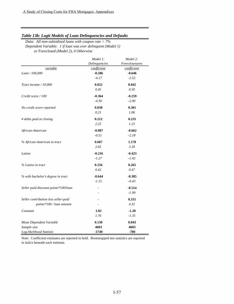
Data: All non-subsidized loans with coupon rate > 7% Dependent Variable: 1 if loan was ever delinquent (Model 1) or Foreclosed (Model 2), 0 Otherwise
Model 1: Delinquencies
Model 2: Foreclosesures
variable coefficient coefficientLoan / 100,000 -0.586 -0.646
-4.17 -2.52
Tract income / 10,000 0.022 0.0420.45 0.50
Credit score / 100 -0.364 -0.259-4.30 -2.00
No credit score reported 0.038 0.3010.21 1.06
# debts paid at closing 0.212 0.2352.25 1.23
African-American -0.087 -0.662-0.51 -2.18
% African-American in tract 0.687 1.1782.65 3.18
Latino -0.216 -0.423-1.27 -1.42
% Latino in tract 0.156 0.2650.42 0.47
% with bachelor's degree in tract -0.644 -0.385-1.15 -0.43
Seller paid discount points*100/loan - -0.514- -1.99
Seller contribution less seller-paid - 0.331 points*100 / loan amount - 4.32
Constant 1.02 -1.201.76 -1.35
Mean Dependent Variable 0.130 0.043Sample size 4603 4603Log-likelihood Statistic -1740 -780
Note: Coefficient estimates are reported in bold. Bootstrapped test statistics are reported in italics beneath each estimate.
Table 13b: Logit Models of Loan Delinquencies and Defaults
A Study of Closing Costs for FHA Mortgages: Appendixes
I-57
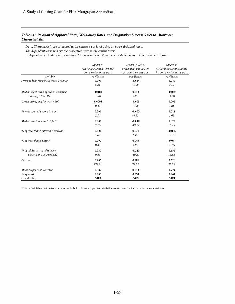
Data: These models are estimated at the census tract level using all non-subsidized loans. The dependent variables are the respective rates in the census tracts Independent variables are the average for the tract when there is more than one loan in a given census tract.
Model 1: Approvals/applications for
borrower's census tract
Model 2: Walk-aways/applications for borrower's census tract
Model 3: Originations/applications
for borrower's census tractvariable coefficient coefficient coefficient
Average loan for census tract/ 100,000 0.009 -0.034 0.0435.31 -6.59 7.10
Median tract value of owner-occupied -0.018 0.012 -0.030 housing / 100,000 -6.70 1.97 -4.08
Credit score, avg for tract / 100 0.0004 -0.005 0.0050.42 -1.90 1.81
% with no credit score in tract 0.006 -0.005 0.0112.74 -0.82 1.63
Median tract income / 10,000 0.007 -0.018 0.02411.23 -13.19 15.43
% of tract that is African-American 0.006 0.071 -0.0651.82 9.69 -7.31
% of tract that is Latino 0.002 0.049 -0.0470.42 4.90 -3.85
% of adults in tract that have 0.037 -0.215 0.252 a bachelors degree (BA) 6.86 -16.24 16.95
Constant 0.905 0.381 0.524122.81 22.53 27.29
Mean Dependent Variable 0.937 0.213 0.724R-squared 0.059 0.259 0.247Sample size 5409 5409 5409
Note: Coefficient estimates are reported in bold. Bootstrapped test statistics are reported in italics beneath each estimate.
Table 14: Relation of Approval Rates, Walk-away Rates, and Origination Success Rates to Borrower Characteristics
A Study of Closing Costs for FHA Mortgages: Appendixes
I-58
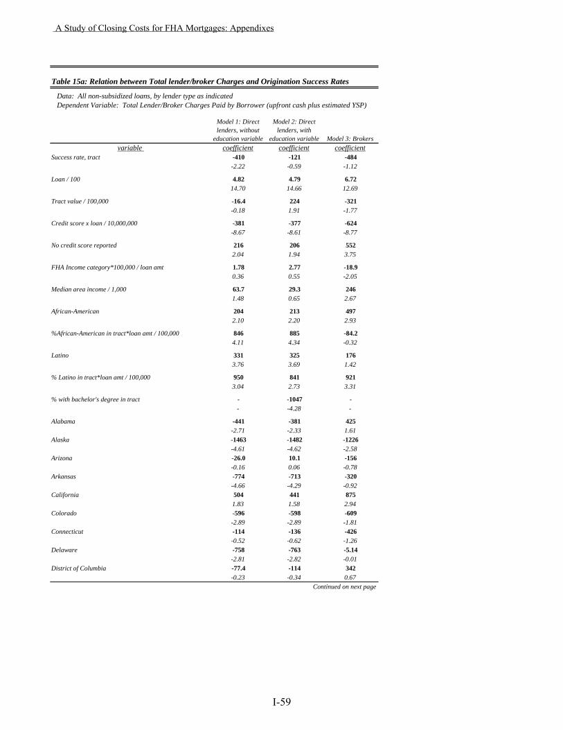
Model 1: Direct lenders, without
education variable
Model 2: Direct lenders, with
education variable Model 3: Brokersvariable coefficient coefficient coefficient
Success rate, tract -410 -121 -484-2.22 -0.59 -1.12
Loan / 100 4.82 4.79 6.7214.70 14.66 12.69
Tract value / 100,000 -16.4 224 -321-0.18 1.91 -1.77
Credit score x loan / 10,000,000 -381 -377 -624-8.67 -8.61 -8.77
No credit score reported 216 206 5522.04 1.94 3.75
FHA Income category*100,000 / loan amt 1.78 2.77 -18.90.36 0.55 -2.05
Median area income / 1,000 63.7 29.3 2461.48 0.65 2.67
African-American 204 213 4972.10 2.20 2.93
%African-American in tract*loan amt / 100,000 846 885 -84.24.11 4.34 -0.32
Latino 331 325 1763.76 3.69 1.42
% Latino in tract*loan amt / 100,000 950 841 9213.04 2.73 3.31
% with bachelor's degree in tract - -1047 -- -4.28 -
Alabama -441 -381 425-2.71 -2.33 1.61
Alaska -1463 -1482 -1226-4.61 -4.62 -2.58
Arizona -26.0 10.1 -156-0.16 0.06 -0.78
Arkansas -774 -713 -320-4.66 -4.29 -0.92
California 504 441 8751.83 1.58 2.94
Colorado -596 -598 -609-2.89 -2.89 -1.81
Connecticut -114 -136 -426-0.52 -0.62 -1.26
Delaware -758 -763 -5.14-2.81 -2.82 -0.01
District of Columbia -77.4 -114 342-0.23 -0.34 0.67
Continued on next page
Data: All non-subsidized loans, by lender type as indicated
Table 15a: Relation between Total lender/broker Charges and Origination Success Rates
Dependent Variable: Total Lender/Broker Charges Paid by Borrower (upfront cash plus estimated YSP)
A Study of Closing Costs for FHA Mortgages: Appendixes
I-59
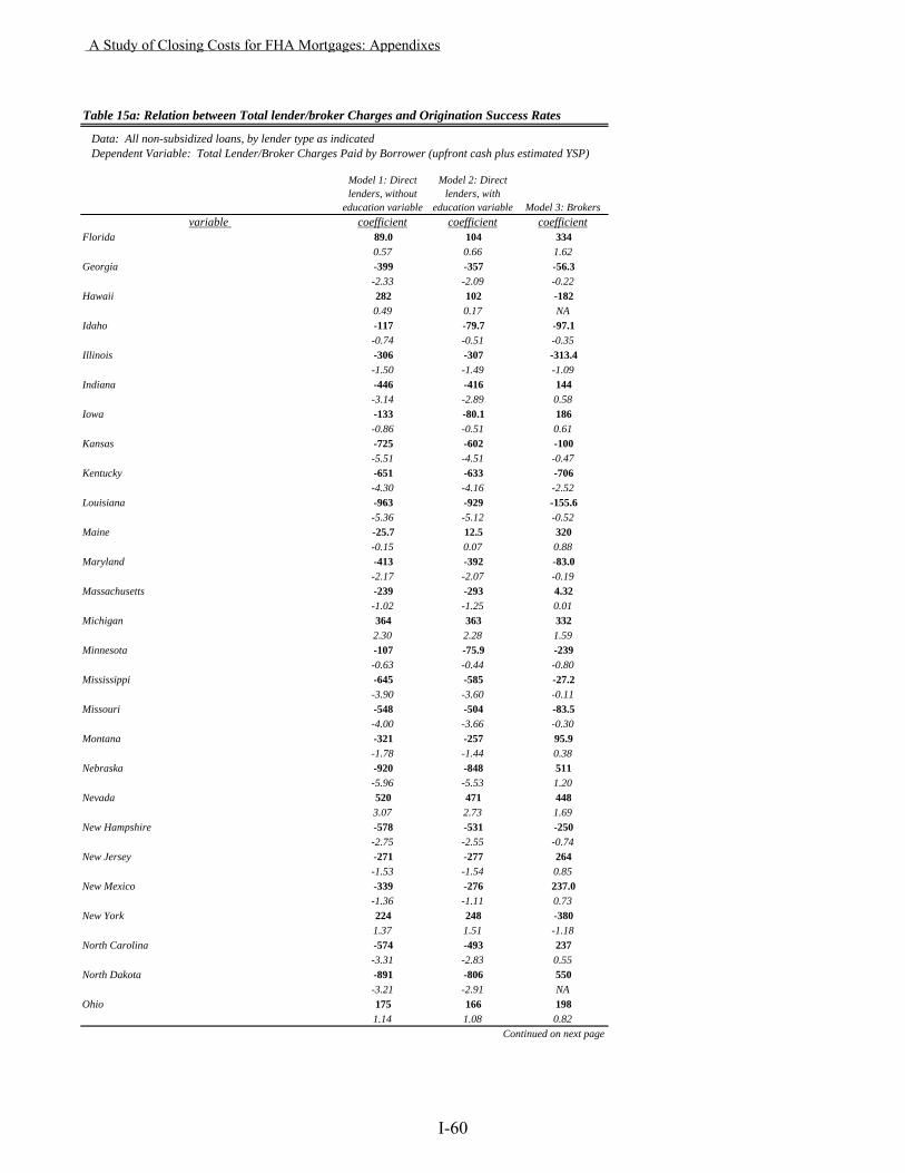
Model 1: Direct lenders, without
education variable
Model 2: Direct lenders, with
education variable Model 3: Brokersvariable coefficient coefficient coefficient
Data: All non-subsidized loans, by lender type as indicated
Table 15a: Relation between Total lender/broker Charges and Origination Success Rates
Dependent Variable: Total Lender/Broker Charges Paid by Borrower (upfront cash plus estimated YSP)
Florida 89.0 104 3340.57 0.66 1.62
Georgia -399 -357 -56.3-2.33 -2.09 -0.22
Hawaii 282 102 -1820.49 0.17 NA
Idaho -117 -79.7 -97.1-0.74 -0.51 -0.35
Illinois -306 -307 -313.4-1.50 -1.49 -1.09
Indiana -446 -416 144-3.14 -2.89 0.58
Iowa -133 -80.1 186-0.86 -0.51 0.61
Kansas -725 -602 -100-5.51 -4.51 -0.47
Kentucky -651 -633 -706-4.30 -4.16 -2.52
Louisiana -963 -929 -155.6-5.36 -5.12 -0.52
Maine -25.7 12.5 320-0.15 0.07 0.88
Maryland -413 -392 -83.0-2.17 -2.07 -0.19
Massachusetts -239 -293 4.32-1.02 -1.25 0.01
Michigan 364 363 3322.30 2.28 1.59
Minnesota -107 -75.9 -239-0.63 -0.44 -0.80
Mississippi -645 -585 -27.2-3.90 -3.60 -0.11
Missouri -548 -504 -83.5-4.00 -3.66 -0.30
Montana -321 -257 95.9-1.78 -1.44 0.38
Nebraska -920 -848 511-5.96 -5.53 1.20
Nevada 520 471 4483.07 2.73 1.69
New Hampshire -578 -531 -250-2.75 -2.55 -0.74
New Jersey -271 -277 264-1.53 -1.54 0.85
New Mexico -339 -276 237.0-1.36 -1.11 0.73
New York 224 248 -3801.37 1.51 -1.18
North Carolina -574 -493 237-3.31 -2.83 0.55
North Dakota -891 -806 550-3.21 -2.91 NA
Ohio 175 166 1981.14 1.08 0.82
Continued on next page
A Study of Closing Costs for FHA Mortgages: Appendixes
I-60
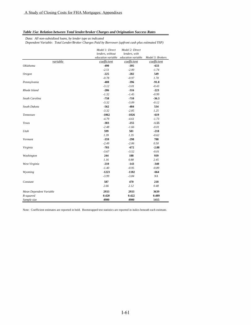
Model 1: Direct lenders, without
education variable
Model 2: Direct lenders, with
education variable Model 3: Brokersvariable coefficient coefficient coefficient
Data: All non-subsidized loans, by lender type as indicated
Table 15a: Relation between Total lender/broker Charges and Origination Success Rates
Dependent Variable: Total Lender/Broker Charges Paid by Borrower (upfront cash plus estimated YSP)
Oklahoma -490 -395 -633-2.51 -2.00 -1.74
Oregon -225 -282 549-0.78 -0.97 1.70
Pennsylvania -408 -396 -91.8-3.12 -3.01 -0.43
Rhode Island -286 -316 -223-1.32 -1.45 -0.99
South Carolina -758 -710 -36.3-3.32 -3.09 -0.12
South Dakota -562 -484 534-3.32 -2.85 1.25
Tennessee -1062 -1026 -619-4.79 -4.61 -1.73
Texas -383 -255 -1.55-2.48 -1.66 -0.01
Utah 599 581 -2181.39 1.35 -0.62
Vermont -359 -298 788-2.49 -2.06 0.50
Virginia -703 -672 -2.88-3.67 -3.52 -0.01
Washington 244 188 9391.16 0.88 2.45
West Virginia -210 -143 -340-1.40 -0.95 -0.89
Wyoming -1223 -1182 -664-3.99 -3.84 NA
Constant 587 470 2182.66 2.12 0.48
Mean Dependent Variable 2933 2933 3639R-squared 0.420 0.422 0.489Sample size 4900 4900 1415
Note: Coefficient estimates are reported in bold. Bootstrapped test statistics are reported in italics beneath each estimate.
A Study of Closing Costs for FHA Mortgages: Appendixes
I-61
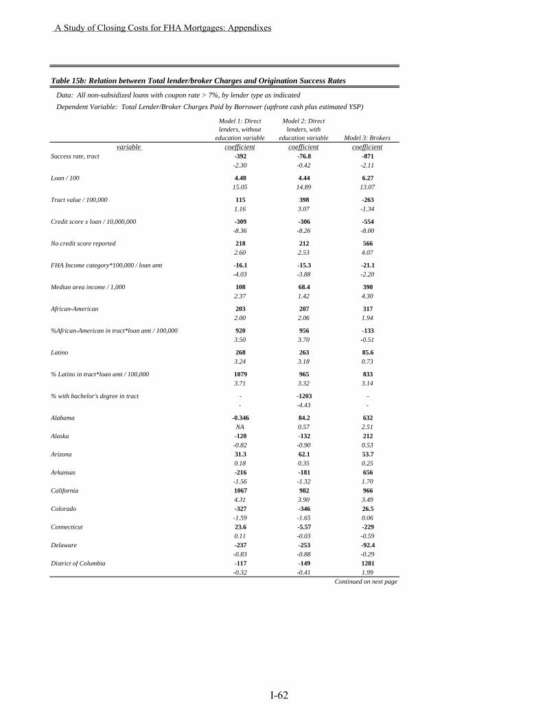
Model 1: Direct lenders, without
education variable
Model 2: Direct lenders, with
education variable Model 3: Brokersvariable coefficient coefficient coefficient
Success rate, tract -392 -76.8 -871-2.30 -0.42 -2.11
Loan / 100 4.48 4.44 6.2715.05 14.89 13.07
Tract value / 100,000 115 398 -2631.16 3.07 -1.34
Credit score x loan / 10,000,000 -309 -306 -554-8.36 -8.26 -8.00
No credit score reported 218 212 5662.60 2.53 4.07
FHA Income category*100,000 / loan amt -16.1 -15.3 -21.1-4.03 -3.88 -2.20
Median area income / 1,000 108 68.4 3902.37 1.42 4.30
African-American 203 207 3172.00 2.06 1.94
%African-American in tract*loan amt / 100,000 920 956 -1333.50 3.70 -0.51
Latino 268 263 85.63.24 3.18 0.73
% Latino in tract*loan amt / 100,000 1079 965 8333.71 3.32 3.14
% with bachelor's degree in tract - -1203 -- -4.43 -
Alabama -0.346 84.2 632NA 0.57 2.51
Alaska -120 -132 212-0.82 -0.90 0.53
Arizona 31.3 62.1 53.70.18 0.35 0.25
Arkansas -216 -181 656-1.56 -1.32 1.70
California 1067 982 9664.31 3.90 3.49
Colorado -327 -346 26.5-1.59 -1.65 0.06
Connecticut 23.6 -5.57 -2290.11 -0.03 -0.59
Delaware -237 -253 -92.4-0.83 -0.88 -0.29
District of Columbia -117 -149 1281-0.32 -0.41 1.99
Continued on next page
Data: All non-subsidized loans with coupon rate > 7%, by lender type as indicated
Table 15b: Relation between Total lender/broker Charges and Origination Success Rates
Dependent Variable: Total Lender/Broker Charges Paid by Borrower (upfront cash plus estimated YSP)
A Study of Closing Costs for FHA Mortgages: Appendixes
I-62
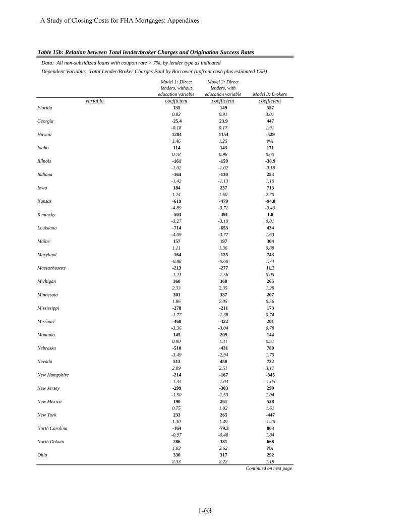
Model 1: Direct lenders, without
education variable
Model 2: Direct lenders, with
education variable Model 3: Brokersvariable coefficient coefficient coefficient
Data: All non-subsidized loans with coupon rate > 7%, by lender type as indicated
Table 15b: Relation between Total lender/broker Charges and Origination Success Rates
Dependent Variable: Total Lender/Broker Charges Paid by Borrower (upfront cash plus estimated YSP)
Florida 135 149 5570.82 0.91 3.01
Georgia -25.4 23.9 447-0.18 0.17 1.91
Hawaii 1284 1154 -5291.46 1.25 NA
Idaho 114 143 1710.78 0.98 0.60
Illinois -161 -159 -38.9-1.02 -1.02 -0.18
Indiana -164 -130 253-1.42 -1.13 1.10
Iowa 184 237 7131.24 1.60 2.70
Kansas -619 -479 -94.8-4.89 -3.71 -0.43
Kentucky -503 -491 1.8-3.27 -3.19 0.01
Louisiana -714 -653 434-4.09 -3.77 1.63
Maine 157 197 3041.11 1.36 0.88
Maryland -164 -125 743-0.88 -0.68 1.74
Massachusetts -213 -277 11.2-1.21 -1.56 0.05
Michigan 360 360 2652.33 2.35 1.28
Minnesota 301 337 2071.86 2.05 0.56
Mississippi -278 -211 173-1.77 -1.38 0.74
Missouri -468 -422 201-3.36 -3.04 0.78
Montana 145 209 1440.90 1.31 0.51
Nebraska -510 -431 780-3.49 -2.94 1.75
Nevada 513 450 7322.89 2.51 3.17
New Hampshire -214 -167 -345-1.34 -1.04 -1.05
New Jersey -299 -303 299-1.50 -1.53 1.04
New Mexico 190 261 5280.75 1.02 1.61
New York 233 265 -4471.30 1.49 -1.26
North Carolina -164 -79.3 803-0.97 -0.48 1.84
North Dakota 286 381 6681.83 2.62 NA
Ohio 330 317 2922.33 2.22 1.19
Continued on next page
A Study of Closing Costs for FHA Mortgages: Appendixes
I-63
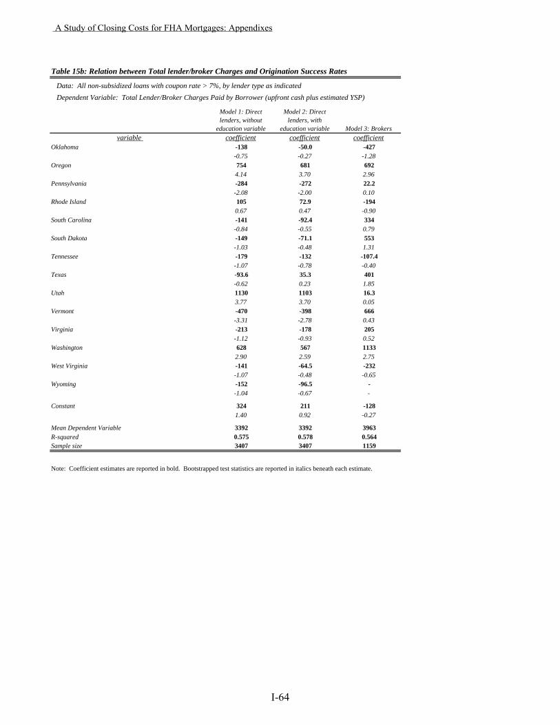
Model 1: Direct lenders, without
education variable
Model 2: Direct lenders, with
education variable Model 3: Brokersvariable coefficient coefficient coefficient
Data: All non-subsidized loans with coupon rate > 7%, by lender type as indicated
Table 15b: Relation between Total lender/broker Charges and Origination Success Rates
Dependent Variable: Total Lender/Broker Charges Paid by Borrower (upfront cash plus estimated YSP)
Oklahoma -138 -50.0 -427-0.75 -0.27 -1.28
Oregon 754 681 6924.14 3.70 2.96
Pennsylvania -284 -272 22.2-2.08 -2.00 0.10
Rhode Island 105 72.9 -1940.67 0.47 -0.90
South Carolina -141 -92.4 334-0.84 -0.55 0.79
South Dakota -149 -71.1 553-1.03 -0.48 1.31
Tennessee -179 -132 -107.4-1.07 -0.78 -0.40
Texas -93.6 35.3 401-0.62 0.23 1.85
Utah 1130 1103 16.33.77 3.70 0.05
Vermont -470 -398 666-3.31 -2.78 0.43
Virginia -213 -178 205-1.12 -0.93 0.52
Washington 628 567 11332.90 2.59 2.75
West Virginia -141 -64.5 -232-1.07 -0.48 -0.65
Wyoming -152 -96.5 --1.04 -0.67 -
Constant 324 211 -1281.40 0.92 -0.27
Mean Dependent Variable 3392 3392 3963R-squared 0.575 0.578 0.564Sample size 3407 3407 1159
Note: Coefficient estimates are reported in bold. Bootstrapped test statistics are reported in italics beneath each estimate.
A Study of Closing Costs for FHA Mortgages: Appendixes
I-64
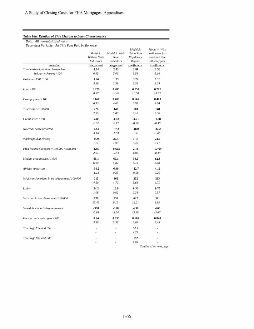
Data: All non-subsidized loans Dependent Variable: All Title Fees Paid by Borrower
Model 1: Without State
Indicators
Model 2: With State
Indicators
Model 3: Using State Regulatory
Regime
Model 4: With indicators for state and title attorney fees
variable coefficient coefficient coefficient coefficientTotal cash origination charges less 4.04 2.53 3.81 2.56 3rd party charges / 100 6.95 5.06 6.58 5.16
Estimated YSP / 100 3.46 1.23 3.24 1.105.99 3.59 6.38 3.24
Loan / 100 0.229 0.285 0.250 0.2878.97 14.46 10.08 14.62
Downpayment / 100 0.660 0.400 0.665 0.4136.13 4.68 5.97 4.94
Tract value / 100,000 220 149 169 1487.55 5.40 6.18 5.36
Credit score / 100 -4.85 -1.18 -4.71 -1.98-0.57 -0.17 -0.56 -0.30
No credit score reported -42.4 -37.2 -48.0 -37.2-1.63 -1.83 -1.91 -1.86
# debts paid at closing 15.9 22.5 7.19 24.21.21 1.99 0.49 2.17
FHA Income Category * 100,000 / loan amt 2.35 -0.603 2.16 -0.4692.01 -0.63 1.88 -0.49
Median area income / 1,000 65.1 60.1 58.5 62.36.69 5.82 6.16 6.08
African-American -30.2 6.90 -22.7 4.12-1.13 0.33 -0.98 0.20
%African-American in tract*loan amt / 100,000 215 262 252 2634.50 4.70 5.68 4.71
Latino 24.2 10.9 8.30 9.751.08 0.62 0.38 0.57
% Latino in tract*loan amt / 100,000 676 333 622 32115.45 9.15 14.21 8.99
% with bachelor's degree in tract -358 -198 -238 -206-5.84 -3.54 -3.98 -3.67
Fees to real estate agent / 100 0.64 0.835 0.665 0.8403.30 5.38 3.69 5.45
Title Reg: File and Use - - 52.2 -- - 4.25 -
Title Reg: Use and File - - 192 -- - 7.69 -
Continued on next page
Table 16a: Relation of Title Charges to Loan Characteristics
A Study of Closing Costs for FHA Mortgages: Appendixes
I-65
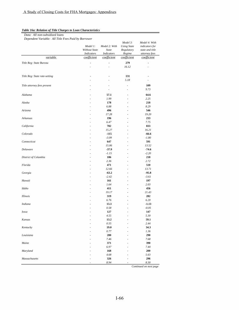
Data: All non-subsidized loans Dependent Variable: All Title Fees Paid by Borrower
Model 1: Without State
Indicators
Model 2: With State
Indicators
Model 3: Using State Regulatory
Regime
Model 4: With indicators for state and title attorney fees
variable coefficient coefficient coefficient coefficient
Table 16a: Relation of Title Charges to Loan Characteristics
Title Reg: State Bureau - - 279 -- - 16.12 -
Title Reg: State rate-setting - - 131 -- - 5.18 -
Title attorney fees present - - - 109- - - 9.73
Alabama - 57.1 - 64.6- 1.99 - 2.25
Alaska - 178 - 218- 6.88 - 8.29
Arizona - 496 - 546- 17.28 - 19.20
Arkansas - 196 - 233- 6.47 - 7.75
California - 782 - 833- 15.27 - 16.21
Colorado - -115 - -66.6- -3.09 - -1.80
Connecticut - 647 - 591- 15.06 - 13.52
Delaware - -37.9 - -74.6- -1.15 - -2.20
District of Columbia - 186 - 218- 2.36 - 2.72
Florida - 471 - 510- 12.66 - 13.71
Georgia - -63.2 - -95.8- -2.42 - -3.61
Hawaii - 161 - 197- 1.64 - 2.03
Idaho - 411 - 456- 19.17 - 21.43
Illinois - 319 - 282- 6.76 - 6.20
Indiana - 13.3 - -1.13- 0.58 - -0.05
Iowa - 127 - 147- 4.55 - 5.30
Kansas - 13.2 - 59.1- 0.55 - 2.44
Kentucky - 19.0 - 34.3- 0.77 - 1.36
Louisiana - 280 - 290- 7.46 - 7.68
Maine - 371 - 390- 6.97 - 7.44
Maryland - 168 - 200- 4.68 - 5.63
Massachusetts - 326 - 296- 8.94 - 8.30
Continued on next page
A Study of Closing Costs for FHA Mortgages: Appendixes
I-66

Data: All non-subsidized loans Dependent Variable: All Title Fees Paid by Borrower
Model 1: Without State
Indicators
Model 2: With State
Indicators
Model 3: Using State Regulatory
Regime
Model 4: With indicators for state and title attorney fees
variable coefficient coefficient coefficient coefficient
Table 16a: Relation of Title Charges to Loan Characteristics
Michigan - 208 - 246- 6.87 - 8.20
Minnesota - 203 - 242- 7.28 - 8.58
Mississippi - 16.4 - -8.94- 0.56 - -0.30
Missouri - -30.4 - 13.2- -1.25 - 0.56
Montana - 316 - 336- 11.51 - 12.77
Nebraska - -42.1 - 1.09- -1.10 - 0.03
Nevada - 232 - 278- 7.34 - 8.78
New Hampshire - 73.8 - 88.3- 2.82 - 3.42
New Jersey - 751 - 728- 17.28 - 17.68
New Mexico - 193 - 231- 5.95 - 6.93
New York - 813 - 785- 14.76 - 14.18
North Carolina - -261 - -280- -9.05 - -9.70
North Dakota - -44.0 - -5.97- -1.28 - -0.18
Ohio - 303 - 300- 7.29 - 7.35
Oklahoma - 565 - 614- 7.91 - 8.62
Oregon - 275 - 322- 10.08 - 12.00
Pennsylvania - 303 - 339- 12.55 - 14.17
Rhode Island - 464 - 457- 14.33 - 14.28
South Carolina - 123 - 88.2- 4.33 - 3.15
South Dakota - 55.0 - 55.3- 1.56 - 1.51
Tennessee - 137 - 165- 4.69 - 5.95
Texas - 810 - 810- 24.93 - 25.39
Utah - 218 - 266- 3.48 - 4.22
Vermont - 254 - 195- 5.68 - 4.37
Virginia - 153 - 155- 5.54 - 5.66
Washington - 503 - 545- 14.14 - 15.58
West Virginia - 145 - 162- 5.08 - 5.80
Continued on next page
A Study of Closing Costs for FHA Mortgages: Appendixes
I-67
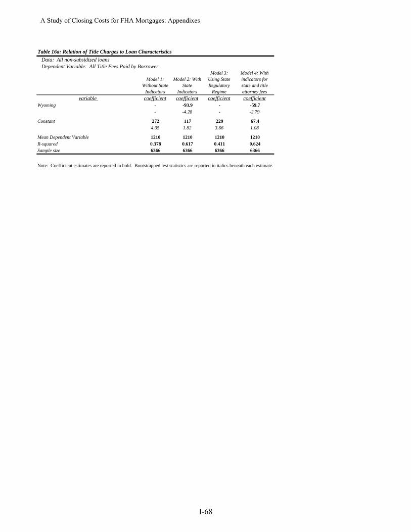
Data: All non-subsidized loans Dependent Variable: All Title Fees Paid by Borrower
Model 1: Without State
Indicators
Model 2: With State
Indicators
Model 3: Using State Regulatory
Regime
Model 4: With indicators for state and title attorney fees
variable coefficient coefficient coefficient coefficient
Table 16a: Relation of Title Charges to Loan Characteristics
Wyoming - -93.9 - -59.7- -4.28 - -2.79
Constant 272 117 229 67.44.05 1.82 3.66 1.08
Mean Dependent Variable 1210 1210 1210 1210R-squared 0.378 0.617 0.411 0.624Sample size 6366 6366 6366 6366
Note: Coefficient estimates are reported in bold. Bootstrapped test statistics are reported in italics beneath each estimate.
A Study of Closing Costs for FHA Mortgages: Appendixes
I-68
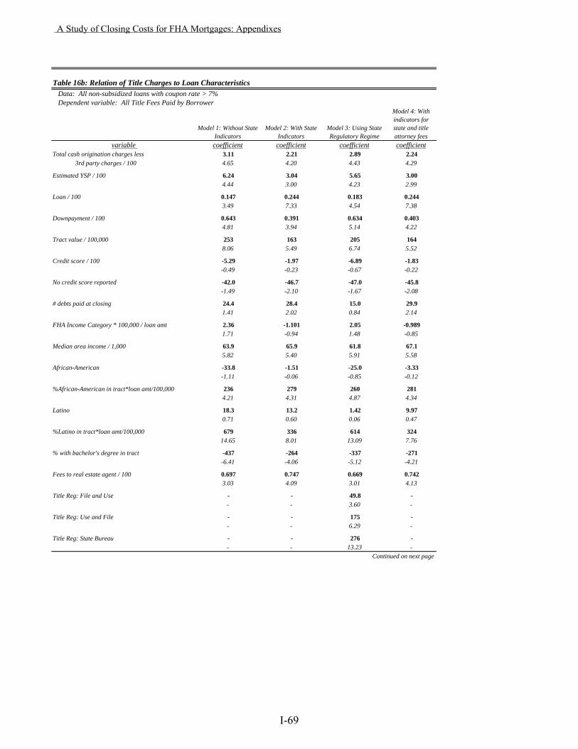
Data: All non-subsidized loans with coupon rate > 7% Dependent variable: All Title Fees Paid by Borrower
Model 1: Without State Indicators
Model 2: With State Indicators
Model 3: Using State Regulatory Regime
Model 4: With indicators for state and title attorney fees
variable coefficient coefficient coefficient coefficientTotal cash origination charges less 3.11 2.21 2.89 2.24 3rd party charges / 100 4.65 4.20 4.43 4.29
Estimated YSP / 100 6.24 3.04 5.65 3.004.44 3.00 4.23 2.99
Loan / 100 0.147 0.244 0.183 0.2443.49 7.33 4.54 7.38
Downpayment / 100 0.643 0.391 0.634 0.4034.81 3.94 5.14 4.22
Tract value / 100,000 253 163 205 1648.06 5.49 6.74 5.52
Credit score / 100 -5.29 -1.97 -6.89 -1.83-0.49 -0.23 -0.67 -0.22
No credit score reported -42.0 -46.7 -47.0 -45.8-1.49 -2.10 -1.67 -2.08
# debts paid at closing 24.4 28.4 15.0 29.91.41 2.02 0.84 2.14
FHA Income Category * 100,000 / loan amt 2.36 -1.101 2.05 -0.9891.71 -0.94 1.48 -0.85
Median area income / 1,000 63.9 65.9 61.8 67.15.82 5.40 5.91 5.58
African-American -33.8 -1.51 -25.0 -3.33-1.11 -0.06 -0.85 -0.12
%African-American in tract*loan amt/100,000 236 279 260 2814.21 4.31 4.87 4.34
Latino 18.3 13.2 1.42 9.970.71 0.60 0.06 0.47
%Latino in tract*loan amt/100,000 679 336 614 32414.65 8.01 13.09 7.76
% with bachelor's degree in tract -437 -264 -337 -271-6.41 -4.06 -5.12 -4.21
Fees to real estate agent / 100 0.697 0.747 0.669 0.7423.03 4.09 3.01 4.13
Title Reg: File and Use - - 49.8 -- - 3.60 -
Title Reg: Use and File - - 175 -- - 6.29 -
Title Reg: State Bureau - - 276 -- - 13.23 -
Continued on next page
Table 16b: Relation of Title Charges to Loan Characteristics
A Study of Closing Costs for FHA Mortgages: Appendixes
I-69
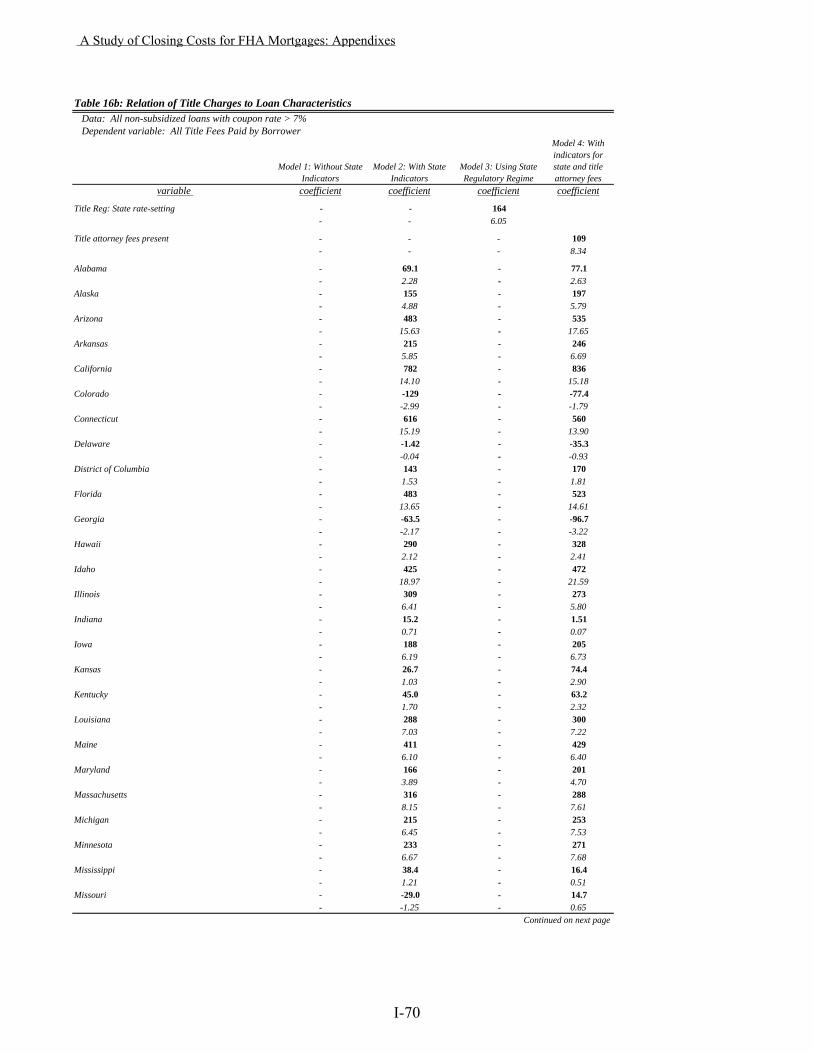
Data: All non-subsidized loans with coupon rate > 7% Dependent variable: All Title Fees Paid by Borrower
Model 1: Without State Indicators
Model 2: With State Indicators
Model 3: Using State Regulatory Regime
Model 4: With indicators for state and title attorney fees
variable coefficient coefficient coefficient coefficient
Table 16b: Relation of Title Charges to Loan Characteristics
Title Reg: State rate-setting - - 164- - 6.05
Title attorney fees present - - - 109- - - 8.34
Alabama - 69.1 - 77.1- 2.28 - 2.63
Alaska - 155 - 197- 4.88 - 5.79
Arizona - 483 - 535- 15.63 - 17.65
Arkansas - 215 - 246- 5.85 - 6.69
California - 782 - 836- 14.10 - 15.18
Colorado - -129 - -77.4- -2.99 - -1.79
Connecticut - 616 - 560- 15.19 - 13.90
Delaware - -1.42 - -35.3- -0.04 - -0.93
District of Columbia - 143 - 170- 1.53 - 1.81
Florida - 483 - 523- 13.65 - 14.61
Georgia - -63.5 - -96.7- -2.17 - -3.22
Hawaii - 290 - 328- 2.12 - 2.41
Idaho - 425 - 472- 18.97 - 21.59
Illinois - 309 - 273- 6.41 - 5.80
Indiana - 15.2 - 1.51- 0.71 - 0.07
Iowa - 188 - 205- 6.19 - 6.73
Kansas - 26.7 - 74.4- 1.03 - 2.90
Kentucky - 45.0 - 63.2- 1.70 - 2.32
Louisiana - 288 - 300- 7.03 - 7.22
Maine - 411 - 429- 6.10 - 6.40
Maryland - 166 - 201- 3.89 - 4.70
Massachusetts - 316 - 288- 8.15 - 7.61
Michigan - 215 - 253- 6.45 - 7.53
Minnesota - 233 - 271- 6.67 - 7.68
Mississippi - 38.4 - 16.4- 1.21 - 0.51
Missouri - -29.0 - 14.7- -1.25 - 0.65
Continued on next page
A Study of Closing Costs for FHA Mortgages: Appendixes
I-70

Data: All non-subsidized loans with coupon rate > 7% Dependent variable: All Title Fees Paid by Borrower
Model 1: Without State Indicators
Model 2: With State Indicators
Model 3: Using State Regulatory Regime
Model 4: With indicators for state and title attorney fees
variable coefficient coefficient coefficient coefficient
Table 16b: Relation of Title Charges to Loan Characteristics
Montana - 335 - 354- 11.20 - 11.99
Nebraska - -27.2 - 14.3- -0.93 - 0.48
Nevada - 232 - 279- 6.84 - 8.31
New Hampshire - 63.2 - 76.9- 2.36 - 2.90
New Jersey - 764 - 743- 16.98 - 17.71
New Mexico - 214 - 250- 6.32 - 7.06
New York - 810 - 784- 14.66 - 14.11
North Carolina - -226 - -245- -6.82 - -7.57
North Dakota - 20.1 - 68.7- 0.49 - 1.70
Ohio - 316 - 311- 6.90 - 6.80
Oklahoma - 564 - 613- 8.70 - 9.37
Oregon - 252 - 301- 8.90 - 10.73
Pennsylvania - 302 - 339- 11.12 - 12.69
Rhode Island - 479 - 469- 13.49 - 13.50
South Carolina - 138 - 96.2- 4.13 - 2.92
South Dakota - 61.0 - 73.0- 1.69 - 1.95
Tennessee - 103 - 130- 2.95 - 3.83
Texas - 777 - 782- 22.62 - 23.16
Utah - 234 - 284- 3.35 - 4.05
Vermont - 265 - 207- 6.13 - 4.86
Virginia - 167 - 170- 5.81 - 5.94
Washington - 520 - 563- 14.81 - 16.12
West Virginia - 160 - 179- 5.62 - 6.45
Wyoming - -88.0 - -59.4- -3.36 - -2.34
Constant 291 100.4 238 47.23.72 1.34 3.26 0.65
Mean Dependent Variable 1227 1227 1227 1227R-squared 0.387 0.618 0.420 0.624Sample size 4603 4603 4603 4603Note: Coefficient estimates are reported in bold. Bootstrapped test statistics are reported in italics beneath each estimate.
A Study of Closing Costs for FHA Mortgages: Appendixes
I-71
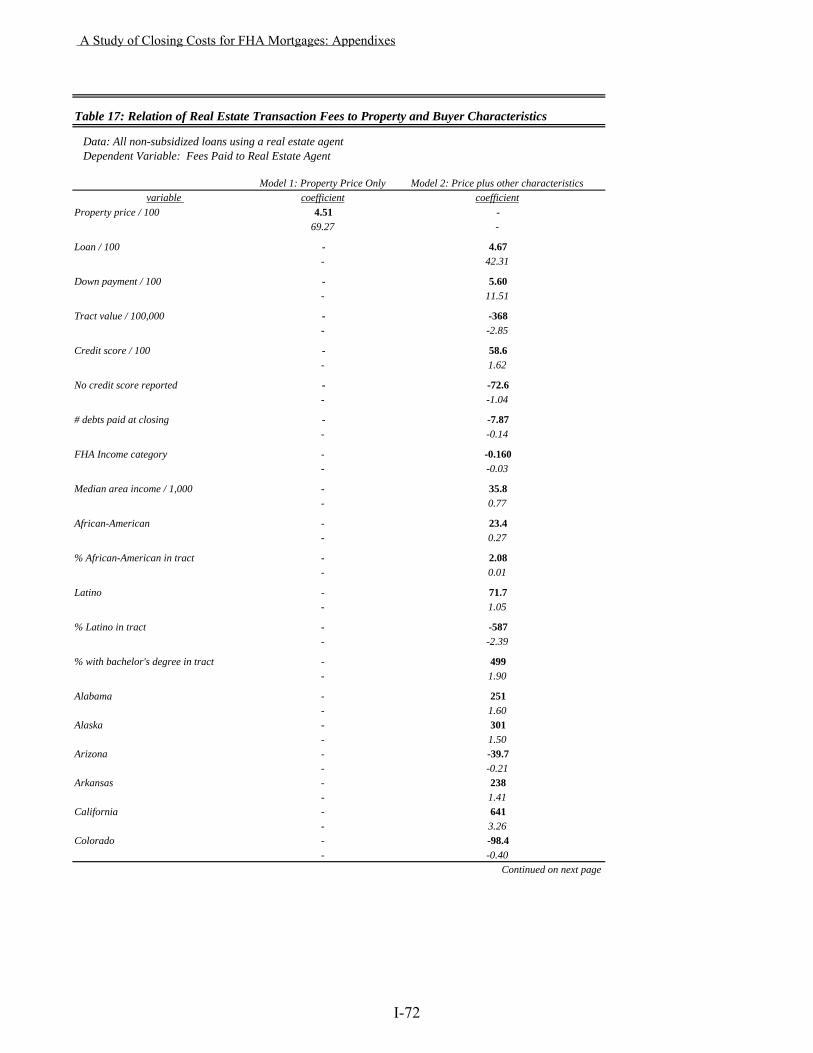
Data: All non-subsidized loans using a real estate agent Dependent Variable: Fees Paid to Real Estate Agent
Model 1: Property Price Only Model 2: Price plus other characteristicsvariable coefficient coefficient
Property price / 100 4.51 -69.27 -
Loan / 100 - 4.67- 42.31
Down payment / 100 - 5.60- 11.51
Tract value / 100,000 - -368- -2.85
Credit score / 100 - 58.6- 1.62
No credit score reported - -72.6- -1.04
# debts paid at closing - -7.87- -0.14
FHA Income category - -0.160- -0.03
Median area income / 1,000 - 35.8- 0.77
African-American - 23.4- 0.27
% African-American in tract - 2.08- 0.01
Latino - 71.7- 1.05
% Latino in tract - -587- -2.39
% with bachelor's degree in tract - 499- 1.90
Alabama - 251- 1.60
Alaska - 301- 1.50
Arizona - -39.7- -0.21
Arkansas - 238- 1.41
California - 641- 3.26
Colorado - -98.4- -0.40
Continued on next page
Table 17: Relation of Real Estate Transaction Fees to Property and Buyer Characteristics
A Study of Closing Costs for FHA Mortgages: Appendixes
I-72

Data: All non-subsidized loans using a real estate agent Dependent Variable: Fees Paid to Real Estate Agent
Model 1: Property Price Only Model 2: Price plus other characteristicsvariable coefficient coefficient
Table 17: Relation of Real Estate Transaction Fees to Property and Buyer Characteristics
Connecticut - 395- 2.59
Delaware - 285- 1.65
District of Columbia - 621- 2.53
Florida - 222- 1.36
Georgia - 794- 4.57
Hawaii - 1056- 2.10
Idaho - 92.1- 0.61
Illinois - -354- -2.00
Indiana - 328- 1.97
Iowa - 611- 4.07
Kansas - 337- 2.14
Kentucky - 58.2- 0.31
Louisiana - 190- 0.95
Maine - 732- 5.11
Maryland - 531- 2.71
Massachusetts - -233- -0.96
Michigan - 435- 2.62
Minnesota - 602- 2.86
Mississippi - -294- -1.72
Missouri - 237- 1.32
Montana - -47.9- -0.28
Nebraska - 691- 4.21
Nevada - 227- 1.14
New Hampshire - 60.7- 0.32
New Jersey - 609- 4.28
New Mexico - 612- 3.21
Continued on next page
A Study of Closing Costs for FHA Mortgages: Appendixes
I-73
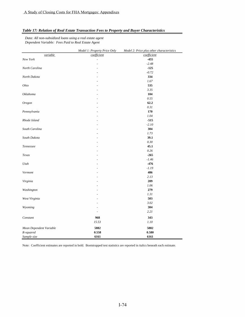
Data: All non-subsidized loans using a real estate agent Dependent Variable: Fees Paid to Real Estate Agent
Model 1: Property Price Only Model 2: Price plus other characteristicsvariable coefficient coefficient
Table 17: Relation of Real Estate Transaction Fees to Property and Buyer Characteristics
New York - -455- -2.48
North Carolina - -125- -0.72
North Dakota - 334- 1.67
Ohio - 535- 3.35
Oklahoma - 104- 0.55
Oregon - 62.2- 0.31
Pennsylvania - 170- 1.04
Rhode Island - -515- -2.10
South Carolina - 304- 1.73
South Dakota - 39.1- 0.30
Tennessee - 45.1- 0.26
Texas - -265- -1.46
Utah - -476- -1.19
Vermont - 486- 2.13
Virginia - 209- 1.06
Washington - 279- 1.31
West Virginia - 503- 3.02
Wyoming - 304- 2.21
Constant 968 34315.53 1.10
Mean Dependent Variable 5882 5882R-squared 0.558 0.580Sample size 6161 6161
Note: Coefficient estimates are reported in bold. Bootstrapped test statistics are reported in italics beneath each estimate.
A Study of Closing Costs for FHA Mortgages: Appendixes
I-74
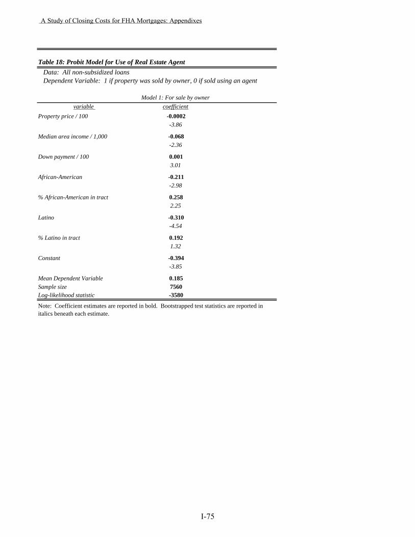
Table 18: Probit Model for Use of Real Estate Agent Data: All non-subsidized loans Dependent Variable: 1 if property was sold by owner, 0 if sold using an agent
Model 1: For sale by ownervariable coefficient
Property price / 100 -0.0002-3.86
Median area income / 1,000 -0.068-2.36
Down payment / 100 0.0013.01
African-American -0.211-2.98
% African-American in tract 0.2582.25
Latino -0.310-4.54
% Latino in tract 0.1921.32
Constant -0.394-3.85
Mean Dependent Variable 0.185Sample size 7560Log-likelihood statistic -3580
Note: Coefficient estimates are reported in bold. Bootstrapped test statistics are reported in italics beneath each estimate.
A Study of Closing Costs for FHA Mortgages: Appendixes
I-75
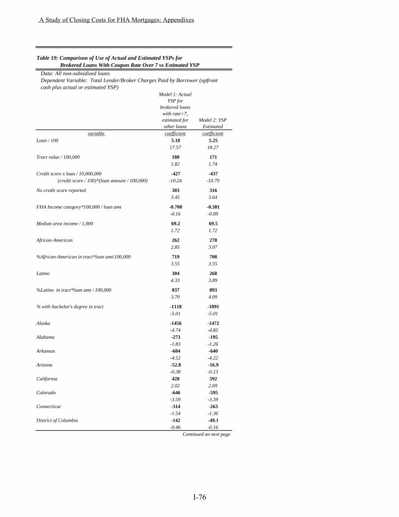
Table 19: Comparison of Use of Actual and Estimated YSPs for Brokered Loans With Coupon Rate Over 7 vs Estimated YSP Data: All non-subsidized loans
cash plus actual or estimated YSP)Model 1: Actual
YSP for brokered loans
with rate>7, estimated for other loans
Model 2: YSP Estimated
variable coefficient coefficientLoan / 100 5.18 5.25
17.57 18.27
Tract value / 100,000 180 1711.82 1.74
Credit score x loan / 10,000,000 -427 -437 (credit score / 100)*(loan amount / 100,000) -10.24 -10.79
No credit score reported 303 3163.45 3.64
FHA Income category*100,000 / loan amt -0.708 -0.381-0.16 -0.09
Median area income / 1,000 69.2 69.51.72 1.72
African-American 262 2782.85 3.07
%African-American in tract*loan amt/100,000 719 7083.55 3.55
Latino 304 2684.33 3.89
%Latino in tract*loan amt / 100,000 837 8933.70 4.09
% with bachelor's degree in tract -1118 -1091-5.01 -5.01
Alaska -1456 -1472-4.74 -4.85
Alabama -273 -195-1.83 -1.26
Arkansas -684 -640-4.52 -4.22
Arizona -52.8 -16.9-0.38 -0.13
California 428 5922.02 2.69
Colorado -646 -595-3.59 -3.39
Connecticut -314 -263-1.54 -1.36
District of Columbia -142 -49.1-0.46 -0.16
Continued on next page
Dependent Variable: Total Lender/Broker Charges Paid by Borrower (upfront
A Study of Closing Costs for FHA Mortgages: Appendixes
I-76
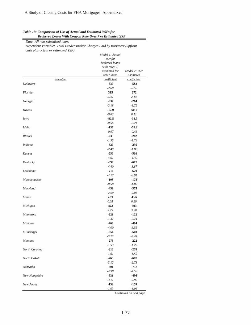
Table 19: Comparison of Use of Actual and Estimated YSPs for Brokered Loans With Coupon Rate Over 7 vs Estimated YSP Data: All non-subsidized loans
cash plus actual or estimated YSP)Model 1: Actual
YSP for brokered loans
with rate>7, estimated for other loans
Model 2: YSP Estimated
variable coefficient coefficient
Dependent Variable: Total Lender/Broker Charges Paid by Borrower (upfront
Delaware -630 -583-2.68 -2.59
Florida 315 2722.30 2.14
Georgia -337 -264-2.18 -1.72
Hawaii -17.9 60.1-0.03 0.11
Iowa -82.5 -31.5-0.56 -0.21
Idaho -137 -59.2-0.97 -0.43
Illinois -233 -282-1.35 -1.72
Indiana -320 -236-2.49 -1.86
Kansas -556 -516-4.61 -4.30
Kentucky -690 -617-4.40 -3.87
Louisiana -716 -679-4.12 -3.91
Massachusetts -108 -178-0.58 -1.03
Maryland -459 -375-2.59 -2.08
Maine 7.74 45.60.05 0.29
Michigan 422 3933.29 3.28
Minnesota -221 -122-1.37 -0.74
Missouri -460 -404-4.00 -3.55
Mississippi -554 -508-3.73 -3.44
Montana -278 -222-1.53 -1.25
North Carolina -310 -278-1.61 -1.52
North Dakota -769 -687-3.12 -2.73
Nebraska -801 -737-4.98 -4.59
New Hampshire -531 -496-3.11 -2.96
New Jersey -159 -159-1.03 -1.06
Continued on next page
A Study of Closing Costs for FHA Mortgages: Appendixes
I-77
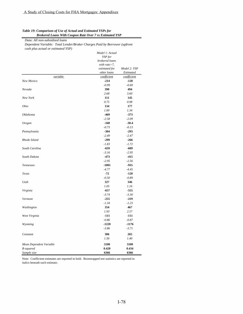
Table 19: Comparison of Use of Actual and Estimated YSPs for Brokered Loans With Coupon Rate Over 7 vs Estimated YSP Data: All non-subsidized loans
cash plus actual or estimated YSP)Model 1: Actual
YSP for brokered loans
with rate>7, estimated for other loans
Model 2: YSP Estimated
variable coefficient coefficient
Dependent Variable: Total Lender/Broker Charges Paid by Borrower (upfront
New Mexico -214 -128-0.99 -0.60
Nevada 390 4942.68 3.60
New York 111 1450.75 0.98
Ohio 134 1771.00 1.34
Oklahoma -469 -373-2.58 -2.09
Oregon -168 -30.4-0.73 -0.13
Pennsylvania -304 -293-2.49 -2.47
Rhode Island -299 -266-1.83 -1.72
South Carolina -659 -609-3.16 -2.95
South Dakota -473 -415-2.95 -2.56
Tennessee -1001 -935-4.77 -4.45
Texas -72 -120-0.50 -0.89
Utah 327 3461.05 1.16
Virginia -657 -555-3.74 -3.30
Vermont -255 -219-1.34 -1.23
Washington 354 4671.93 2.57
West Virginia -111 -111-0.86 -0.87
Wyoming -1220 -1176-3.86 -3.71
Constant 306 2651.56 1.40
Mean Dependent Variable 3100 3100R-squared 0.420 0.434Sample size 6366 6366
Note: Coefficient estimates are reported in bold. Bootstrapped test statistics are reported in italics beneath each estimate.
A Study of Closing Costs for FHA Mortgages: Appendixes
I-78
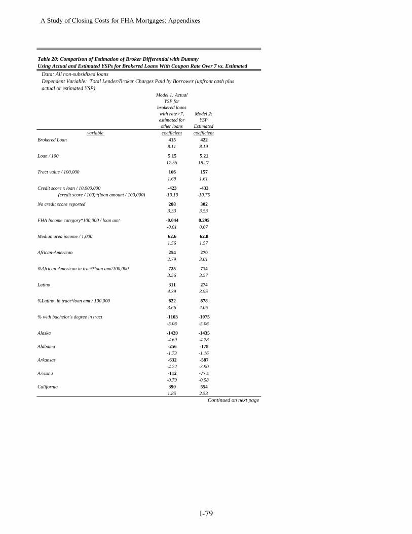
Table 20: Comparison of Estimation of Broker Differential with Dummy Using Actual and Estimated YSPs for Brokered Loans With Coupon Rate Over 7 vs. Estimated Data: All non-subsidized loans
actual or estimated YSP)Model 1: Actual
YSP for brokered loans
with rate>7, estimated for other loans
Model 2: YSP
Estimatedvariable coefficient coefficient
Brokered Loan 415 4228.11 8.19
Loan / 100 5.15 5.2117.55 18.27
Tract value / 100,000 166 1571.69 1.61
Credit score x loan / 10,000,000 -423 -433 (credit score / 100)*(loan amount / 100,000) -10.19 -10.75
No credit score reported 288 3023.33 3.53
FHA Income category*100,000 / loan amt -0.044 0.295-0.01 0.07
Median area income / 1,000 62.6 62.81.56 1.57
African-American 254 2702.79 3.01
%African-American in tract*loan amt/100,000 725 7143.56 3.57
Latino 311 2744.39 3.95
%Latino in tract*loan amt / 100,000 822 8783.66 4.06
% with bachelor's degree in tract -1103 -1075-5.06 -5.06
Alaska -1420 -1435-4.69 -4.78
Alabama -256 -178-1.73 -1.16
Arkansas -632 -587-4.22 -3.90
Arizona -112 -77.1-0.79 -0.58
California 390 5541.85 2.53
Continued on next page
Dependent Variable: Total Lender/Broker Charges Paid by Borrower (upfront cash plus
A Study of Closing Costs for FHA Mortgages: Appendixes
I-79
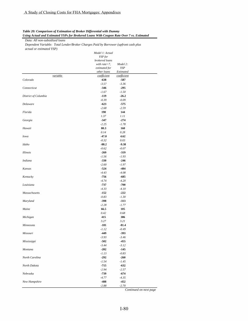
Table 20: Comparison of Estimation of Broker Differential with Dummy Using Actual and Estimated YSPs for Brokered Loans With Coupon Rate Over 7 vs. Estimated Data: All non-subsidized loans
actual or estimated YSP)Model 1: Actual
YSP for brokered loans
with rate>7, estimated for other loans
Model 2: YSP
Estimatedvariable coefficient coefficient
Dependent Variable: Total Lender/Broker Charges Paid by Borrower (upfront cash plus
Colorado -638 -587-3.57 -3.36
Connecticut -346 -295-1.67 -1.50
District of Columbia -119 -26.2-0.39 -0.09
Delaware -623 -575-2.68 -2.59
Florida 190 1441.37 1.11
Georgia -347 -274-2.25 -1.78
Hawaii 80.3 1600.14 0.28
Iowa -47.0 4.62-0.32 0.03
Idaho -88.2 -9.38-0.62 -0.07
Illinois -269 -319-1.56 -1.93
Indiana -330 -246-2.60 -1.97
Kansas -524 -484-4.43 -4.08
Kentucky -756 -685-4.74 -4.20
Louisiana -737 -700-4.33 -4.10
Massachusetts -152 -222-0.83 -1.30
Maryland -398 -313-2.28 -1.77
Maine 66.5 1050.42 0.68
Michigan 415 3863.27 3.21
Minnesota -181 -81.4-1.12 -0.49
Missouri -449 -393-3.93 -3.46
Mississippi -502 -455-3.44 -3.12
Montana -202 -145-1.13 -0.83
North Carolina -292 -260-1.54 -1.45
North Dakota -715 -632-2.94 -2.57
Nebraska -739 -674-4.77 -4.35
New Hampshire -488 -452-2.88 -2.70
Continued on next page
A Study of Closing Costs for FHA Mortgages: Appendixes
I-80

Table 20: Comparison of Estimation of Broker Differential with Dummy Using Actual and Estimated YSPs for Brokered Loans With Coupon Rate Over 7 vs. Estimated Data: All non-subsidized loans
actual or estimated YSP)Model 1: Actual
YSP for brokered loans
with rate>7, estimated for other loans
Model 2: YSP
Estimatedvariable coefficient coefficient
Dependent Variable: Total Lender/Broker Charges Paid by Borrower (upfront cash plus
New Jersey -130 -130-0.85 -0.87
New Mexico -182 -95.8-0.85 -0.46
Nevada 362 4662.43 3.30
New York 137 1710.92 1.14
Ohio 148 1911.13 1.46
Oklahoma -433 -337-2.32 -1.87
Oregon -187 -50.0-0.81 -0.22
Pennsylvania -318 -307-2.64 -2.60
Rhode Island -334 -300-2.04 -1.94
South Carolina -605 -554-2.94 -2.72
South Dakota -403 -344-2.56 -2.17
Tennessee -971 -905-4.69 -4.35
Texas -87.6 -136-0.62 -1.02
Utah 286 3050.91 1.00
Virginia -612 -510-3.51 -3.06
Vermont -189 -152-1.02 -0.88
Washington 330 4441.80 2.44
West Virginia -94.9 -94.2-0.74 -0.73
Wyoming -1130 -1084-3.61 -3.46
Constant 247 2041.27 1.09
Mean Dependent Variable 3100 3100R-squared 0.428 0.443Sample size 6366 6366
Note: Coefficient estimates are reported in bold. Bootstrapped test statistics are reported in italics beneath each estimate.
A Study of Closing Costs for FHA Mortgages: Appendixes
I-81
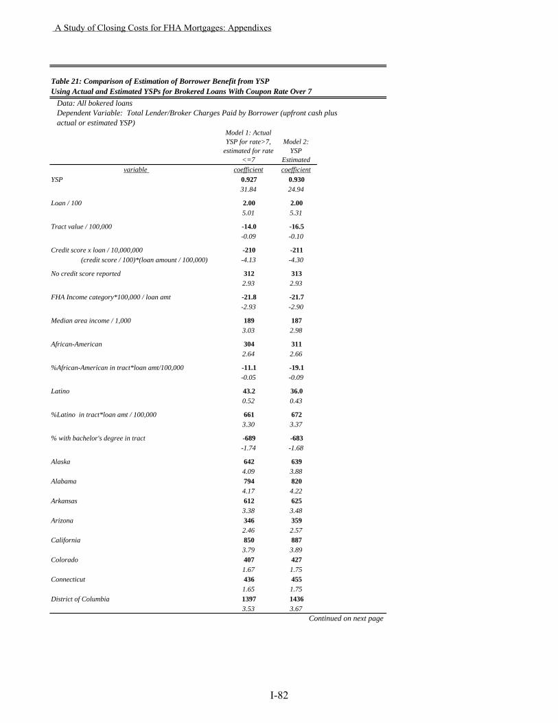
Table 21: Comparison of Estimation of Borrower Benefit from YSP Using Actual and Estimated YSPs for Brokered Loans With Coupon Rate Over 7 Data: All bokered loans
actual or estimated YSP)Model 1: Actual YSP for rate>7,
estimated for rate <=7
Model 2: YSP
Estimatedvariable coefficient coefficient
YSP 0.927 0.93031.84 24.94
Loan / 100 2.00 2.005.01 5.31
Tract value / 100,000 -14.0 -16.5-0.09 -0.10
Credit score x loan / 10,000,000 -210 -211 (credit score / 100)*(loan amount / 100,000) -4.13 -4.30
No credit score reported 312 3132.93 2.93
FHA Income category*100,000 / loan amt -21.8 -21.7-2.93 -2.90
Median area income / 1,000 189 1873.03 2.98
African-American 304 3112.64 2.66
%African-American in tract*loan amt/100,000 -11.1 -19.1-0.05 -0.09
Latino 43.2 36.00.52 0.43
%Latino in tract*loan amt / 100,000 661 6723.30 3.37
% with bachelor's degree in tract -689 -683-1.74 -1.68
Alaska 642 6394.09 3.88
Alabama 794 8204.17 4.22
Arkansas 612 6253.38 3.48
Arizona 346 3592.46 2.57
California 850 8873.79 3.89
Colorado 407 4271.67 1.75
Connecticut 436 4551.65 1.75
District of Columbia 1397 14363.53 3.67
Continued on next page
Dependent Variable: Total Lender/Broker Charges Paid by Borrower (upfront cash plus
A Study of Closing Costs for FHA Mortgages: Appendixes
I-82
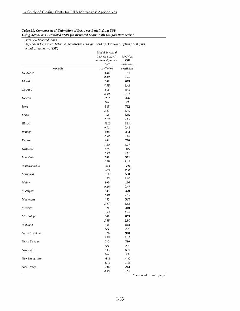
Table 21: Comparison of Estimation of Borrower Benefit from YSP Using Actual and Estimated YSPs for Brokered Loans With Coupon Rate Over 7 Data: All bokered loans
actual or estimated YSP)Model 1: Actual YSP for rate>7,
estimated for rate <=7
Model 2: YSP
Estimatedvariable coefficient coefficient
Dependent Variable: Total Lender/Broker Charges Paid by Borrower (upfront cash plus
Delaware 136 1510.40 0.45
Florida 668 6694.38 4.43
Georgia 816 8414.90 5.11
Hawaii -202 -142NA NA
Iowa 685 7023.21 3.30
Idaho 551 5862.77 2.83
Illinois 79.2 75.40.51 0.48
Indiana 408 4342.52 2.65
Kansas 203 2161.20 1.27
Kentucky 474 4962.99 3.07
Louisiana 560 5713.09 3.19
Massachusetts -191 -200-0.84 -0.88
Maryland 510 5501.93 2.06
Maine 100 1060.38 0.41
Michigan 385 3792.38 2.32
Minnesota 485 5272.47 2.62
Missouri 321 3401.63 1.73
Mississippi 840 8592.88 2.90
Montana 485 518NA NA
North Carolina 976 9883.08 3.17
North Dakota 732 780NA NA
Nebraska 503 531NA NA
New Hampshire -442 -435-1.75 -1.69
New Jersey 206 2040.95 0.93
Continued on next page
A Study of Closing Costs for FHA Mortgages: Appendixes
I-83
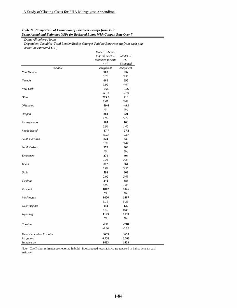
Table 21: Comparison of Estimation of Borrower Benefit from YSP Using Actual and Estimated YSPs for Brokered Loans With Coupon Rate Over 7 Data: All bokered loans
actual or estimated YSP)Model 1: Actual YSP for rate>7,
estimated for rate <=7
Model 2: YSP
Estimatedvariable coefficient coefficient
Dependent Variable: Total Lender/Broker Charges Paid by Borrower (upfront cash plus
New Mexico 903 9373.20 3.30
Nevada 668 6953.92 4.07
New York -165 -156-0.63 -0.59
Ohio 705.2 7193.65 3.63
Oklahoma -89.6 -49.4NA NA
Oregon 884 9214.99 5.22
Pennsylvania 164 1680.98 1.00
Rhode Island -37.7 -27.1-0.23 -0.17
South Carolina 824 8453.35 3.47
South Dakota 775 808NA NA
Tennessee 379 4042.24 2.39
Texas 872 8646.07 5.96
Utah 591 6032.02 2.09
Virginia 342 3860.95 1.08
Vermont 1042 1046NA NA
Washington 1456 14875.15 5.29
West Virginia 141 1370.50 0.48
Wyoming 1123 1139NA NA
Constant -211 -218-0.80 -0.82
Mean Dependent Variable 3653 3653R-squared 0.739 0.706Sample size 1433 1433
Note: Coefficient estimates are reported in bold. Bootstrapped test statistics are reported in italics beneath each estimate.
A Study of Closing Costs for FHA Mortgages: Appendixes
I-84
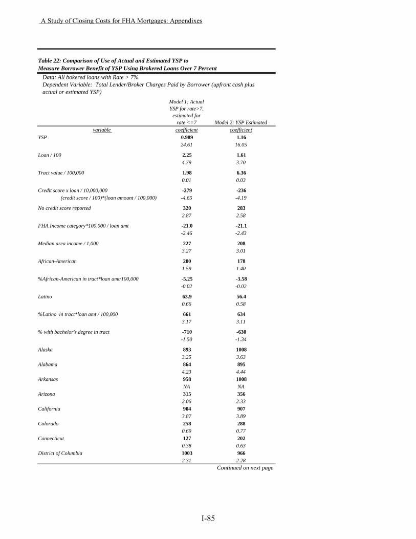
Table 22: Comparison of Use of Actual and Estimated YSP to Measure Borrower Benefit of YSP Using Brokered Loans Over 7 Percent Data: All bokered loans with Rate > 7%
actual or estimated YSP)Model 1: Actual YSP for rate>7,
estimated for rate <=7 Model 2: YSP Estimated
variable coefficient coefficientYSP 0.989 1.16
24.61 16.05
Loan / 100 2.25 1.614.79 3.70
Tract value / 100,000 1.98 6.360.01 0.03
Credit score x loan / 10,000,000 -279 -236 (credit score / 100)*(loan amount / 100,000) -4.65 -4.19
No credit score reported 320 2832.87 2.58
FHA Income category*100,000 / loan amt -21.0 -21.1-2.46 -2.43
Median area income / 1,000 227 2083.27 3.01
African-American 200 1781.59 1.40
%African-American in tract*loan amt/100,000 -5.25 -3.58-0.02 -0.02
Latino 63.9 56.40.66 0.58
%Latino in tract*loan amt / 100,000 661 6343.17 3.11
% with bachelor's degree in tract -710 -630-1.50 -1.34
Alaska 893 10083.25 3.63
Alabama 864 8954.23 4.44
Arkansas 958 1008NA NA
Arizona 315 3562.06 2.33
California 904 9073.87 3.89
Colorado 258 2880.69 0.77
Connecticut 127 2020.38 0.63
District of Columbia 1003 9662.31 2.28
Continued on next page
Dependent Variable: Total Lender/Broker Charges Paid by Borrower (upfront cash plus
A Study of Closing Costs for FHA Mortgages: Appendixes
I-85

Table 22: Comparison of Use of Actual and Estimated YSP to Measure Borrower Benefit of YSP Using Brokered Loans Over 7 Percent Data: All bokered loans with Rate > 7%
actual or estimated YSP)Model 1: Actual YSP for rate>7,
estimated for rate <=7 Model 2: YSP Estimated
variable coefficient coefficient
Dependent Variable: Total Lender/Broker Charges Paid by Borrower (upfront cash plus
Delaware 139 1760.41 0.52
Florida 722 7464.73 4.93
Georgia 717 7524.73 5.10
Hawaii 16.0 142NA NA
Iowa 899 9143.96 4.09
Idaho 481 525NA NA
Illinois 202 2421.27 1.55
Indiana 489 5192.83 3.06
Kansas 216 2491.21 1.39
Kentucky 496 5692.37 2.74
Louisiana 707 7423.28 3.38
Massachusetts -197 -228-0.83 -0.95
Maryland 702 6902.23 2.32
Maine 127 87.20.49 0.34
Michigan 348 3532.13 2.18
Minnesota 366 3881.14 1.20
Missouri 416 4452.19 2.39
Mississippi 522 5622.14 2.16
Montana 552 598NA NA
North Carolina 1181 12202.99 3.13
North Dakota 869 907NA NA
Nebraska 577 530NA NA
New Hampshire -379 -417-1.43 -1.57
New Jersey 173 1400.75 0.61
Continued on next page
A Study of Closing Costs for FHA Mortgages: Appendixes
I-86

Table 22: Comparison of Use of Actual and Estimated YSP to Measure Borrower Benefit of YSP Using Brokered Loans Over 7 Percent Data: All bokered loans with Rate > 7%
actual or estimated YSP)Model 1: Actual YSP for rate>7,
estimated for rate <=7 Model 2: YSP Estimated
variable coefficient coefficient
Dependent Variable: Total Lender/Broker Charges Paid by Borrower (upfront cash plus
New Mexico 987 10313.10 3.19
Nevada 739 7384.12 4.10
New York -227 -202-0.83 -0.74
Ohio 671.7 7323.19 3.45
Oklahoma 16.2 90.3NA NA
Oregon 931 9784.86 5.24
Pennsylvania 16.4 12.50.10 0.08
Rhode Island -98.9 -83.6-0.57 -0.48
South Carolina 964 1047NA NA
South Dakota 772 790NA NA
Tennessee 364 4281.71 2.01
Texas 794 8225.23 5.46
Utah 657 7641.89 2.13
Virginia 321 3550.80 0.88
Vermont 1123 1164NA NA
Washington 1362 14114.19 4.44
West Virginia 128 1520.41 0.49
Wyoming NA NANA NA
Constant -356.2 -325-1.21 -1.11
Mean Dependent Variable 3977 3977R-squared 0.727 0.685Sample size 1174 1174
Note: Coefficient estimates are reported in bold. Bootstrapped test statistics are reported in italics beneath each estimate.
A Study of Closing Costs for FHA Mortgages: Appendixes
I-87
A Study of Closing Costs for FHA Mortgages: Appendixes
Appendix II: References
II-1

A Study of Closing Costs for FHA Mortgages: Appendixes
REFERENCES
Aguiar, Mark, and Erik Hurst. 2005. “Expenditure and Consumption.” Journal of Political Economy 113(5): 919–48.
El Anshasy, Amany, Gregory Elliehausen, and Yoshiaki Shimazaki, 2004. “Mortgage Brokers and the Subprime Market” May 2004, available at http://www.ftc.gov/be/seminardocs/0405elliehausen.pdf
Asabere, Paul K. and Forrest E. Hoffman. 1997. “Discount Point Concessions and the Value of Homes with Conventional versus Nonconventional Mortgage Financing” Journal of Real Estate Finance and Economics 15(3): 261–70.
Ayres, Ian. 2001. Pervasive Prejudice? Unconventional Evidence of Race and Gender Discrimination. Chicago, IL: University of Chicago Press.
Ayres, Ian, and Peter Seigelman. 1995. “Race and Gender Discrimination in Bargaining for a New Car.” American Economic Review 85(3): 304–21.
Becker, Gary S. 1957. The Economics of Discrimination, Chicago, IL: University of Chicago Press
Black, Harold A., Thomas P. Boehm, and Ramon P. DeGennaro. 2001a. “Is There Discrimination in Mortgage Pricing? The Case of Overages.” Working Paper 2001-4a. Atlanta, GA: Federal Reserve Bank of Atlanta.
———. 2001b. “Overages, Mortgage Pricing and Race.” Working Paper. Knoxville: University of Tennessee.
Brueckner, J. K. 1994. “Borrower mobility, Adverse Selection, and Mortgage Points.” Journal of Financial Mediation 3(4): 416–41.
Busse, Meghan, Jorge Silva-Risso, and Florian Zettelmeyer. 2006. “$1,000 Cash Back: The Pass-Through of Auto Manufacturer Promotions.” American Economic Review 96(4).
Cohen, Mark A. 2006. “Imperfect Competition in Auto Lending: Subjective Markup, Racial Disparity, and Class Action Litigation.” Law and Economics Research Paper 07-01. Nashville, TN: Owen Graduate School of Management, Vanderbilt University.
Cotterman, Robert F. 1992. Final Report: Seller Financing of Temporary Buydowns, Washington, DC: U.S. Department of Housing and Urban Development.
II-2
A Study of Closing Costs for FHA Mortgages: Appendixes
———. 2001. Neighborhood Effects in Mortgage Default Risk. Washington, DC: U.S. Department of Housing and Urban Development, Office of Policy Development and Research.
———. 2004 Analysis of FHA Single Family Default and Loss Rates. Washington, DC: U.S. Department of Housing and Urban Development, Office of Policy Development and Research.
Courchane, Marsha, and David Nickerson. 1997. “Discrimination Resulting from Overage Practices.” Journal of Financial Services Research 11: 133–51.
Courchane, Marsha, Brian Surette, and Peter Zorn. 2003. “Subprime Borrowers: Mortgage Transitions and Outcomes.” Journal of Real Estate Finance and Economics.
Deng, Yonghing, and Stuart Gabriel. 2005. “Are Underserved Borrowers Lower Risk? New Evidence on the Performance and Pricing of FHA-Insured Mortgages.” Working paper. Los Angeles: Lusk Center for Real Estate, University of Southern California.
Lacko, James M., and Janis K. Pappalardo. 2007. “Improved Consumer Mortgage Disclosures: An Empirical Assessment of Current and Prototype Disclosure Forms.” Bureau of Economics Staff Report. Washington, DC: Federal Trade Commission. Available at http://www.ftc.gov/os/2007/06/P025505MortgageDisclosureReport.pdf.
LaCour-Little, Michael. 1999. “Discrimination in Mortgage Lending: A Critical Review of the Literature.” Journal of Real Estate Literature 7: 15–49.
Morton, Fiona Scott, Florian Zettelmeyer, and Jorge Silva-Risso. 2003. “Consumer Information and Discrimination: Does the Internet Affect the Pricing of New Cars to Women and Minorities?” Quantitative Marketing and Economics 1(1): 65–92.
———. 2007. “What Matters for Price Negotiation: Evidence from the U.S. Auto Retailing Industry.” July. Working paper. http://flomac.haas.berkeley.edu/~florian/Papers/carsurvey.pdf
Shroder, Mark D. 2007. “The Value of Sunshine Cure: The Efficacy of the Real Estate Settlement Procedures Act Disclosure Strategy.” Cityscape: A Journal of Policy Development and Research 9(1): 73–92.
Stango, Victor, and Jonathan Zinman. 2006. “How a Cognitive Bias Shapes Competition: Evidence from Consumer Credit Markets.” http://ssrn.com/abstract=928956.
Stanton, Richard, and Nancy Wallace. 1998. “Mortgage Choice: What’s the Point?” Real Estate Economics 26: 173–205.
II-3
A Study of Closing Costs for FHA Mortgages: Appendixes
Steiner, Faye. 2000. “Quantifying Discrimination in Home Mortgage Lending: Estimation of Loan Price Elasticities across Products and Races.” SIEPR Discussion Paper 00-15. Stanford, CA: Stanford University.
Woodward, Susan E. 2003. “Consumer Confusion in the Mortgage Market” Working Paper, Sand Hill Econometrics
Zorn, Peter, and Robert Van Order. 2001. “Performance of Low Income and Minority Mortgages.” Working paper. Washington, DC: Freddie Mac.
II-4

A Study of Closing Costs for FHA Mortgages: Appendixes
Appendix III: Data
III-1
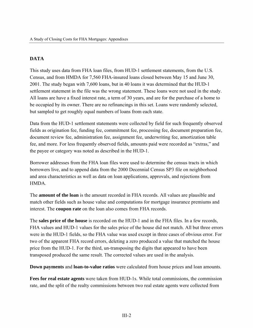
A Study of Closing Costs for FHA Mortgages: Appendixes
DATA
This study uses data from FHA loan files, from HUD-1 settlement statements, from the U.S. Census, and from HMDA for 7,560 FHA-insured loans closed between May 15 and June 30, 2001. The study began with 7,600 loans, but in 40 loans it was determined that the HUD-1 settlement statement in the file was the wrong statement. These loans were not used in the study. All loans are have a fixed interest rate, a term of 30 years, and are for the purchase of a home to be occupied by its owner. There are no refinancings in this set. Loans were randomly selected, but sampled to get roughly equal numbers of loans from each state.
Data from the HUD-1 settlement statements were collected by field for such frequently observed fields as origination fee, funding fee, commitment fee, processing fee, document preparation fee, document review fee, administration fee, assignment fee, underwriting fee, amortization table fee, and more. For less frequently observed fields, amounts paid were recorded as “extras,” and the payee or category was noted as described in the HUD-1.
Borrower addresses from the FHA loan files were used to determine the census tracts in which borrowers live, and to append data from the 2000 Decennial Census SP3 file on neighborhood and area characteristics as well as data on loan applications, approvals, and rejections from HMDA.
The amount of the loan is the amount recorded in FHA records. All values are plausible and match other fields such as house value and computations for mortgage insurance premiums and interest. The coupon rate on the loan also comes from FHA records.
The sales price of the house is recorded on the HUD-1 and in the FHA files. In a few records, FHA values and HUD-1 values for the sales price of the house did not match. All but three errors were in the HUD-1 fields, so the FHA value was used except in three cases of obvious error. For two of the apparent FHA record errors, deleting a zero produced a value that matched the house price from the HUD-1. For the third, un-transposing the digits that appeared to have been transposed produced the same result. The corrected values are used in the analysis.
Down payments and loan-to-value ratios were calculated from house prices and loan amounts.
Fees for real estate agents were taken from HUD-1s. While total commissions, the commission rate, and the split of the realty commissions between two real estate agents were collected from
III-2
A Study of Closing Costs for FHA Mortgages: Appendixes
HUD-1s in addition to the amounts paid by buyer and seller, only the amounts paid by the buyer and seller were subject to the arithmetic test to assure that individual items summed to the total cash required at closing. Thus, the fields relied on were amounts paid by the buyer and by the seller, plus extras payable to real estate agents on the HUD-1 (also subject to the arithmetic test) and amounts paid to realtors outside closing. “Extras” that were not included in agent’s compensation were taxes on agent’s commissions, referral fees to other agents, and extraordinary items such as 1031 exchange fees. Sales tax was shown to be paid on 164 loans, and referral fees were reported on 23 loans. A total of 1,399 loans, or 19 percent, showed no real estate fees, and are presumed to be houses sold by their owners without the assistance of an agent, known in the industry as for-sale-by-owner, or fizbos.
Origination Fees
Origination fees were computed by summing the individual origination items, treating negative amounts in either the standard categories or the “extras” as credits. Credits in the 200 lines of the HUD-1 were also treated as credits, but only if they were contributions from the lender or broker to the borrower’s closing costs. Credits from homeownership programs such as Nehemiah or Ameridream, or various state and local programs, were not counted as reductions in settlement costs. Items payable to settlement service providers for extraordinary items, such as 1031 exchange fee services, premium homeowner’s insurance policies, sales taxes on settlement services, and so on, were also not included as loan origination or title charges.
Third-party charges for credit reports, appraisals, tax service and flood certifications were not included in lender/broker origination fees. Three of these services—appraisal, credit report, and flood certification—are required on FHA loans and all are provided by third parties. FHA lenders are not required to hire third parties for tax servicing, but all FHA lenders must monitor the payment of property taxes. Some lender/servicers subcontract the monitoring and payment of property taxes, and many do not. There were explicit charges for tax service on about half the loans studied here. Many loans were lacking charges for at least one of these third-party items. It is presumed that lenders fulfilled the requirements, and that on loans where there was no itemized charge, lenders absorbed the cost. Thus, to compute lender/broker origination fees on similar terms for all loans, the median charge for loans in the same state was subtracted from lender/broker fees if the explicit charge was not present.
III-3
A Study of Closing Costs for FHA Mortgages: Appendixes
The courier fees for the 900s and 1000s lines of the HUD-1 were included in lender/broker fees, while courier fees and notary fees in the 1200s and 1300s were included in title charges.
There were three different category names for loan discount fees: “loan discount,” “buydown,” and “additional discount.” The three were added together to compute the total loan discount charge. These are the same as discount points.
Yield-spread premium: Three terms were often seen on HUD-1s indicating a payment to a mortgage broker from a wholesale lender: “yield-spread premium,” “service release premium,” and “broker premium.” Eight of these were entered as negative amounts. Because the YSP is paid by the lender to the broker, it was not subject to the arithmetic check on the HUD-1. For purposes of this analysis, the signs of all YSPs were changed to positive. There were 114 loans with more than one type of premium payment recorded (e.g., a yield spread premium and a service release premium). The two premiums were added together to obtain the total yield-spread premium. There were 1,525 loans with reported yield-spread premiums. For the 1,525 loans with reported YSPs, the YSP averaged $2,262.
All loans with YSPs reported are presumed to be loans originated by mortgage brokers. This treatment is likely to miss some brokered loans and to make brokered and direct loans look more similar than they actually are since loans made by brokers where no YSP was recorded are counted as direct loans. This issue is discussed further in the analysis of the data.
The lender is identified on every loan in the FHA loan files. There are 1,799 unique lenders represented in this data. In addition to the broker/direct lender classification, lenders were classified based on name and the number of loans from that lender in our file as depositories, large mortgage banks (> 100 loans in our file), and smaller mortgage banks (< 100 loans). These classifications are largely congruent with the size of these institutions from other data.
Seller contributions to origination fees were computed by summing the seller-paid amounts only, again treating negative entries as credits. Fees for credit reports, appraisals, flood certifications, and tax service were omitted from loan origination fees, as were the same fees paid by buyers. Seller-paid points were obtained by summing the seller-paid amounts to the three categories of discount points.
III-4
A Study of Closing Costs for FHA Mortgages: Appendixes
Title Fees
Total title fees were computed by adding the total amounts paid by the buyer and the seller in the 1100s section of the HUD-1 to title companies and settlement agents, and adding any courier fees and notary fees from the 1200s and 1300s. Seller’s contribution to title fees is simply the separate seller’s total. Attorney’s fees for title paid by the buyer and the seller in connection with the title process were totaled separate from other title charges. Attorney’s fees that were extraordinary to the title process, such as those needed in the case of an estate or divorce, were not included in the total.
Other information gathered from the HUD-1 settlement statements was the number and amount of loan payoffs included in the settlement. Items paid off may be previous mortgages, consumer loans, credit card loans, and second mortgages. Both the total dollar amount paid off and the number of items paid off were gathered.
The FHA files included other useful information about borrowers and their loans. Borrower age is recorded; whether the borrower is a first-time homebuyer; whether borrower is married; gender of the borrower; and categories for borrower income (category 1 is incomes up to $15,000, Category 2 is incomes between $15,000 and $30,000, and additional categories are in $5,000 increments up to Category 35). Borrower race is also recorded. The files also contained information about whether borrowers received loan counseling about the borrowing process. Borrower counseling is classified as lender counseling, third-party counseling, or borrower declined counseling. Counseling data were missing for nine percent of the loans, so this forms a fourth category. Credit score data was taken from FHA loan files. For some loans, more than one credit score was available. When more than one score was recorded, the average of the scores was used. For 420 loans, the borrower had no credit score.
Census Data
The U.S. 2000 Decennial Census has several different demographic measures that were useful in this study. One is median area income. For addresses in metropolitan areas, the study uses median metropolitan area income for the metro area in which the borrower lives. For addresses in nonmetropolitan areas, county median income for the county where borrower lives is used for median area income.
III-5

A Study of Closing Costs for FHA Mortgages: Appendixes
Other useful census variables are educational attainment in the borrower’s census tract, measured as the fraction of adults in the census tract with a bachelor’s. Another is neighborhood house values, measured as the median value of owner-occupied houses in the borrower’s census tract. Neighborhood household income is measured as the median household income in the borrower’s census tract. The racial composition of the neighborhood was measured as the fraction of individuals who are white, African American, or Latino (Hispanic).
HMDA Data
HMDA data are collected based on 1990 census tract boundaries, while the other census data used in this study comes from census tracts as they were drawn for the 2000 decennial census. Borrower addresses were matched to both. It was possible to use data when loans matched to the same census tract for both 1990 and 2000. For these loans, the fields gathered were the number of loan applications, loan originations, and rejected loans for FHA and conventional loans, by census tract for the 7,501 loans that matched to the same tract for both the 1990 and 2000 census.
Delinquency and Foreclosure Data
This book of loans was, at the time of this analysis, over six years old, sufficient to see the pattern of delinquencies and foreclosures. Actual delinquencies and foreclosures were gathered from FHA records.
III-6
A Study of Closing Costs for FHA Mortgages: Appendixes
Appendix IV: Review of Prior Research on Title Fees
IV-1

A Study of Closing Costs for FHA Mortgages: Appendixes
Review of Previous Writing and Research on Title Fees Robert M. Feinberg, Professor of Economics, American University This appendix discusses writings and research on the U.S. market for title services. The title services market has been controversial for many years. Part of the goal of the Real Estate Settlement Procedures Act of 1975 was to prohibit referral fees, rebates, or kickbacks in settlement services generally, but a substantial part of the impetus for RESPA was that title companies wanted relief from the pressure for referral fees from real estate agents and lenders. Investigations and reports at both the federal and state levels continue to identify high prices; market concentration; payment of referral fees, rebates, and kickbacks; and price discrimination as issues in the market for title services (GAO 2006, 2007; Birnbaum 2005).
Two views of title services come through in the writings to be reviewed. One is the view of economists, especially Bruce Owen (1977) and Lawrence White (1984). In their view, the price of title services is held above cost by a combination of industry practices and state regulation. Because prices are artificially held above cost, title companies compete for business by paying referral fees or kickbacks to real estate agents and/or lenders who bring title business to them.
Owen and White contend that despite monopoly pricing in title services, competition in realty agency and lending can deliver competitive pricing to consumers. The other settlement service providers who receive payments from title companies then compete among another and drive their own profits, including the revenue from title companies, to zero. Any inhibition on the payment of referral fees, such as section 8 of RESPA, interferes with the achievement of competitive pricing for consumers. Owen and White see section 8 of RESPA as perverse, inhibiting a force that could deliver competitive pricing to consumers despite cartel pricing in title services.
After the passage of RESPA in 1975, real estate agents and lenders began to establish affiliations with title services through either partial or full ownership of title agencies. This route around section 8 in principle enabled the profit in title transactions to be at least partially captured by a single organization (the combination of real estate agents or lenders with title agencies) without explicit payment of a referral fee. In the economists’ view, this is efficient given the prohibition on explicit referral fees, and might also deliver competitive pricing. The amendments to RESPA in 1983 were an effort to inhibit affiliations between title agents and real estate agents or lenders, called “controlled business arrangements” or “affiliated business arrangements.”
The alternative view, that of the title services industry, is that title service providers have been pressured by real estate agents and lenders to pay them referral fees, kickbacks, or rebates. These referral fees are, for the title agencies, a cost of doing business. This “reverse competition” raises their costs, and they must raise their prices to cover this cost.
IV-2

A Study of Closing Costs for FHA Mortgages: Appendixes
In the economists’ view, the artificial elevation of price above cost invites the payment of kickbacks or referral fees. Economists see what the industry calls “reverse competition” as simply a competition for the profits in title services created by artificially high prices. In the industry’s view, the pressure for referral fees or kickbacks raises costs and, thus, prices.
Title Services
Title insurance service providers include title insurers and title agents, as well as closing (settlement) and escrow service providers. The exact role of each participant varies from state to state and even by metropolitan area within states, but the basic services provided remain the same. The economic importance of title costs is shown by the fact that title charges account for almost 30 percent of cash loan origination and closing fees on a typical real estate transaction (GAO 2007), and by the finding in this report that title charges average $1,200 per loan.
Title services involve searching the history of legal and tax documents pertaining to a property (the title search), evaluating the likelihood of “defects” in the title (e.g., liens against the property), arranging for a title insurance policy to be written (either on the value of the mortgage—a lender’s policy—or on the total value of the property, with the possibility of this covering appreciation as well), and providing the actual insurance.1 Beyond this, as discussed by Lipshutz (1994, 7),
The expense component of title insurance is expanded even further by the fact that the title insurer is frequently also responsible for the closing of the real estate transaction, a responsibility that encompasses correction of any really serious title problems prior to closing; drafting, or at least collecting, all the relevant documents, including deeds and mortgages; maintaining the escrow account; conducting the settlement itself; and recording the documents establishing the new ownership, releasing the mortgage liens of lenders who have been repaid, and recording the lien interests of the new lenders.
The title search itself traditionally involved a time-consuming investigation through documents at a county courthouse, but larger title insurers and agents developed and
maintained their own title plants—a physical housing of title-related documents. Over the past few decades, title plants have become, to a large extent, computerized and title insurers have merged title plants into joint title plants. These joint title plants provide access to other title insurers and underwritten title companies—non-owners—for a subscription fee. Title plant information comes from individual counties as the title-related information—such as property sales,
IV-3
A Study of Closing Costs for FHA Mortgages: Appendixes
liens, and tax information—is filed initially within the county. (Birnbaum 2005, 12)
The 2007 GAO report details considerable variation across states in methods (and efficiency) of title searching: in New York, title agents send employees to various county offices to conduct document searches manually and a “typical title insurance issuance took 90 to 120 days for a purchase and 30 to 45 days for a refinance.” In contrast, for an automated title plant in Texas, “typical turnaround time for a completed title search, examination, and commitment for a title examiner simultaneously working on several titles was 2 to 3 days” (p. 17).
The rationale generally provided by the industry for premiums far in excess of losses is that title search is costly, both in fixed (maintenance of title plants) and variable (labor expenses, primarily) costs.2 Title insurers argue that this extensive search keeps losses low. Of course, there is a classic principal-agent problem here in that the ultimate purchaser of title insurance has no idea how much search is really required to bring expected losses to a reasonable level and must rely on the title agent to do the optimal amount of search.3 While Baker and colleagues (2002, 148) state that “title insurers have a strong interest in ensuring that the search is optimal,” they give no explanation for why title insurers’ interests would be the same as society’s. They find, in a cross-state analysis, that a higher risk of defects is a determinant of longer—and presumably more expensive—search, and interpret this as consistent with efficient search. But Baker and colleague’s empirical proxy for this higher defect risk is simply the average title insurance premium in a state. So, the finding of a positive correlation between premium and search effort could instead be interpreted as suggesting that the title industry simply uses more search as a justification for higher rates.
Structure of Fees
Title insurance fees vary considerably across states. Based on a 2005 Bankrate.com survey of closing costs on a $180,000 loan to urban buyers, Holden Lewis reports that these costs ranged from $439 in North Carolina to $1,451 in New York, similar to the findings in this study.4 However, several factors make comparisons of price schedules across states difficult. First, the services covered by a title insurance premium may differ from state to state. In some states, the premium covers title search by an agent (and possibly additional paperwork and settlement expenses), while in others only the actual insurance is covered, and the title agent charges separately for the title search.5 Second, different rates apply to owners’ (covering buyers on the value of the property as long as they own the particular property) and lenders’ policies (covering lenders up to the value of the loan only until the loan is paid off, either through sale of the property or refinancing). Finally, there are also generally discounts available (though not always offered to homeowners), “reissue rates,” on refinancings.
IV-4
A Study of Closing Costs for FHA Mortgages: Appendixes
Birnbaum (2005, 17) reports:
The bulk of the title insurance premium goes to expenses as opposed to claim payments. A.M. Best reports that title insurers paid an average of 4.6% of premium for claims and claim settlement expenses from 1995 to 2004 compared to around 80% for the property casualty industry.
…..
The title insurance premium is split between the title insurance company and the underwritten title company, when an underwritten title company is involved in the title transaction. The typical premium split in California is 8% to 12% for the title insurer and 92% to 88% for the underwritten title company …[comparable to a title agency in other states]… The percentage of gross title premium retained by title insurers in California—a bit less than 10% on average—is much less than the percentage retained by the same title insurers in other states.6
Commission rates (or split of premiums between title insurers and agents) are generally unregulated and simply reflect negotiations between insurer and agent. Exceptions are Florida, New Mexico, Texas, Connecticut and South Carolina (Lipshutz 1994). The agent can be an employee, an affiliated agency, or an independent agent. According to Lipshutz (1994), more than half of all title insurance premiums are written by independent agents; the agent often does more than just marketing and serves an underwriting function (producing “a fully examined and insurable title”). Even on the marketing side, the agent’s efforts are directed not to ultimate consumers but to local real estate professionals.
Customer loyalty runs primarily to the producer, not the insuring company as such, and so competition among insurers for established producers is intense. In some cases, established title producers can be induced to become employees of an insurer branch office. But many very effective producers prefer to conduct business as independent agents, and in the competition to attract these agents, the primary competitive tool is the commission rate. As institutional loyalties throughout the economy have eroded, switching among insurers by agents has become more common and has led to the perception that prevailing commission rates have crept upward. (Lipshutz 1994, 35–36)
Rate Determination
Fay (2005) summarizes the current mechanisms of regulation of title insurance rates, which vary considerably from state to state. There are 36 “file and use” states, in which title insurers must file rates with the state regulatory body (and often wait for a short time —15–30 days—for either regulatory approval or lack of objections) before using them. Insurers in Alaska, Arizona,
IV-5
A Study of Closing Costs for FHA Mortgages: Appendixes
Nevada, New Jersey, New York, Oregon, and Pennsylvania can avoid separately filing by joining a licensed rating bureau. Three states (Florida, New Mexico, and Texas) directly promulgate rates for insurers within their jurisdictions. Three others (Hawaii, Vermont, and Wisconsin) ask insurers to file or make rates available for inspection but do not require them to wait for approval. Iowa does not allow the sale of title insurance. The remaining states have no rate filing requirements for title insurers.
Roussel and Rosenberg, two lawyers with strong ties to the title insurance industry, defend title insurance price-fixing via rating bureaus. They state (1981, 646), “Title insurance rating bureaus at present provide rate computation for all of their members, based upon consolidated industry data.” Lipshutz (1994) notes that the dominant price scheme in the 1972–1985 period was the rating bureau mechanism—voluntary associations of title insurers to file joint rates for members in “file and use” states—but that this largely ceased in 1985 after an FTC antitrust complaint (which argued that the McCarran-Ferguson exemption did not protect them). According to Nyce and Boyer (1998, 227), “On June 12, 1992, in FTC vs. Ticor Title Insurance Co. et al., the U.S. Supreme Court sided with the FTC in finding that rate bureaus were guilty of horizontal price fixing for title searches and examinations.” While the decision provided some guidance on how rate bureaus could be reformed—essentially, to make them less industry cartel and more directly state regulated—they have become less important since the decision (though they remain in the seven states mentioned above).
Birnbaum (2005, 15) explains that in California,
The price a consumer pays for title insurance is based on rates filed by title insurers with the California Department of Insurance. Rates for title insurance are typically a function of the amount of liability. The liability is the amount of coverage, which is the amount of the loan for the lender’s policy and the purchase price of the house for the owner’s policy. The filed title insurance rates typically do not vary within the state. However, because title rates are a function of sales price or loan amount, the average title premium varies considerably by county.
Similarly, Arrunada (2002, 587) states:
Premiums differ substantially across states. They usually increase in a lower proportion than the amount insured. According to a 1997 survey, for a property valued at 50,000 U.S. dollars, the owner’s policy costs on average 3.55 per thousand, but this falls to 2.44 per thousand for properties valued at one million dollars. These premiums do not include the costs of search (estimated between $192.72 and $519.03), closing services and document preparation.
Roussel and Rosenberg (1981, 645) agree on the basic pattern of pricing:
IV-6
A Study of Closing Costs for FHA Mortgages: Appendixes
The cost of production of a policy does not vary consistently with the exposure for loss; the same cost may be incurred on a policy for a $1,000,000 industrial project and a $50,000 single-family residence. However, the single most important variable in the price of a title insurance policy is its face amount: the typical price structure is ‘x’ dollars per thousand dollars of coverage. Because of the relatively constant cost of production, the result is a substantial cross-subsidization of purchasers of small, single-family, residential policies by purchasers of large facilities, typically commercial, industrial, or large residential developments.7
The 2007 GAO report notes disagreement among industry officials and state regulators as to whether this subsidization was intentional or not.
Price Discrimination by Title Service Providers
Price discrimination is defined by economists as pricing differences to different consumers not justified by cost differences. The discussion above makes clear the systematic price discrimination present in the industry. Because both title insurance premiums and escrow fees generally rise with loan value (while costs, if they rise at all, do so only modestly), owners of higher-valued properties are discriminated against relative to owners of lower-valued properties.8 Whatever one may think of the fairness aspects of this price discrimination, it strongly suggests an absence of competitive forces in the market (this is discussed in more detail below).
In addition, there are less systematic aspects of price discrimination present in favor of better-informed consumers. Reissue rates with discounts of 50 percent or more on refinancing transactions are not always offered to consumers: those who ask get them.9 But given the limited title searching required on refinancings, it is likely that the costs associated with these policies fall by much more than the premiums, implying price discrimination against refinancers (despite the discounts). Similarly purchasers of properties recently sold would seem to be discriminated against given the limited amount of search required to find title defects since the previous sale.
Both the Woodward (2003) and Courchane, McManus, and Zorn (2004) papers deal with broker fees and yield-spread premiums, with no separate discussion of title services and fees. But they do both suggest that homebuyers can be segmented into types by degree of sophistication and that this translates into different fees paid. From the perspective of title fees, this strongly supports the ability to price discriminate by title insurers and agents as well.
IV-7
A Study of Closing Costs for FHA Mortgages: Appendixes
Reverse Competition, Referral Fees, and Controlled Businesses
A feature of the market for title services that is often the focus of discussion is “reverse competition.” Birnbaum (2005, p. 2) describes the basics well:
Title insurance and escrow markets are characterized by reverse competition where the marketing of the products is directed at the real estate agents, mortgage brokers and lenders who steer and direct the home purchaser or borrower—the consumer who actually pays for title and escrow services—to particular title insurers, underwritten title companies and escrow companies. Residential consumers have little, if any, market power because title insurance and escrow services are required for the closing of a real estate transaction, resulting in inelastic demand. In a reverse competitive market, expenses are inflated as title insurers compete for the producers of title business—the real estate agents, mortgage brokers and lenders and others involved in real estate settlements.
However, Birnbaum observes:
Peat Marwick’s study [for HUD] found that ‘the combination of reverse competition and prices set by historical and customary practices has led to excess revenues which either are used to obtain referrals or contribute to underwriter profit.’ The study also concluded that excess profits may not accrue to title insurers, but rather to the producers of the title business. The underwriter may be forced to bid away the excess profits to acquire the business from the real estate settlement entity. (2005, 33)
Referral fees (otherwise known as kickbacks, rebates, or bribes) result from high prices, despite being illegal under RESPA section 8. However, enforcement of RESPA has led to the growth of “controlled businesses” or what the 2007 GAO report refers to as “affiliated business arrangements” (or ABAs, the term that replace “controlled business arrangements”). Owen and Grundfest (1977) note that the potential for collusive profits combined with anti-rebate laws have prompted entry by these “controlled firms”—title insurers and/or title agencies owned by real estate brokerages (and sometimes lenders).
The American Land Title Association’s (ALTA’s) 1979 paper, The Controlled Business Problem in the Title Insurance Industry, argues that a controlled title insurance agency faces little competition and therefore is unlikely to worry about keeping prices low. (ALTA refers to controlled title insurance agencies as ones owned or affiliated with a real estate broker or lender.) They also note that these arrangements create entry barriers for new title insurance service providers into the market.
IV-8
A Study of Closing Costs for FHA Mortgages: Appendixes
Lipshutz has a concise discussion of the relevant issues. Referring to Owen and Grundfest (1977), he suggests “the payment of kickbacks [or referral fees] is an efficient way to market, the profits earned through kickback mechanisms are applied by the kickback recipient to reduce the prices it charges for its other services, and any misbehavior on the part of the kickback recipient is forestalled by the recipient’s regard for its business reputation” (Lipshutz 1994, 68). And, when real estate businesses have opened title insurance agencies (controlled businesses) in response to RESPA, Lipshutz reports that some argue “the profits earned on title insurance agency business are used to subsidize the cost of the other real estate activities of the controlled business agent, and thus reduce the price for other services related to real estate transfer, if not the title insurance rate itself” (Lipshutz 1994, 66, referring to White 1984).
However, Lipshutz goes on to note that others
maintain that controlled business agents extract monopoly rents from their control of customers by charging a higher than necessary commission, or by extorting special concessions from their insurer. With respect to ultimate consumers, they maintain that controlled business agents exploit their monopoly of information by failing to alert purchasers to the existence of lower title insurance rates offered by insurers for whom they do not act as agents, or even from their active insurer through available discounts for special conditions. (Lipshutz 1994, 66)
But the latter point is important. It is only because of monopoly power in related services, especially by brokers, that these rebates or referral fees are not translated into lower prices to consumers. White contends that even successful enforcement of section 8 simply reallocates rents between the various real estate service providers with no change in the price of title insurance to homebuyers if all aspects of settlement services were characterized by monopoly power. “Instead, the title insurers would keep a larger share of the potential profits that the large price-cost margins promised; referrers would receive less” (White 1984, 313).
White also contends that if there were competition among the referrers of business to title insurers (brokers, lenders, lawyers), the ability to get referral fees (reverse competition), by lowering insurers’ cost, would push them to lower prices on their services to consumers. Even without price competition among these providers, they might still compete on non-price measures to the benefit of consumers. Section 8 of RESPA limits this and thus likely makes consumers worse off. White sees controlled businesses as a second-best response to RESPA section 8. Controlled businesses will still need to compete (either in price or non-price ways) to attract consumers, though White does acknowledge that there may be inefficiencies in combining the various providers into a single entity.
More recently, Martin and Ludwick (2006) conclude that title agents within ABAs do not charge higher fees to consumers than independent title agents. Nevertheless, the 2007 GAO report finds
IV-9
A Study of Closing Costs for FHA Mortgages: Appendixes
that “the concerns expressed by regulators and some industry participants over ABAs raise questions about the potential effects of some ABAs on consumers” (p. 33).
Recent Developments Involving Allegations of Title Insurance Kickbacks and Captive Reinsurance Arrangements
A GAO report discusses state and federal investigations of these activities, in particular the practice of captive reinsurance deals. “In such arrangements, a home-builder, real estate broker, lender, title insurance company, or some combination of these entities forms a reinsurance company that works in conjunction with a title insurer. The title insurer agrees to ‘reinsure’ all or part of its business with the reinsurer by paying the company a portion of the premium … for each title transaction” (GAO 2006, 14). Given the minimal risk involved in title insurance, with less than 5 percent of premiums going to pay losses on average, regulators have questioned the need for reinsurance.10
That same GAO report chronicles recent settlements involving HUD as well as cases brought by state insurance regulators in California, New York, and Colorado. It describes the “typical fraudulent business arrangement” as one involving
a shell title agency that is set up by a title agent but that generally has no physical location, employees, or assets, and does not actually perform title and settlement business. In cases we examined, regulators alleged their primary purpose is to serve as a vehicle to provide kickbacks by being a pass-through for payments or preferential treatment given by the title agent to real estate agents and brokers, home-builders, attorneys, or mortgage brokers for business referrals. Investigations have alleged that the arrangements in these cases violate RESPA. (GAO 2006, 15)
One example of a recent settlement involves two leading title insurers—Fidelity National Financial and First American—that each agreed to pay $2 million and reduce rates by 15 percent. The New York Attorney General contended “the insurers drove up rates for homeowners by providing developers free or discounted insurance in other states in exchange for client referrals in New York.”11
The 2007 GAO report identifies “13 [state and HUD] investigations [from 2003 to 2006] involving 37 entities that were related to captive reinsurance arrangements, with 1 multistate settlement agreement involving activities in 26 states” (p. 30). Based on “details provided in a multistate settlement, insurers were allegedly giving away [to reinsurers] as much as one-third or more of the premiums consumers paid in order to obtain consumer referrals,” suggesting to state
IV-10
A Study of Closing Costs for FHA Mortgages: Appendixes
regulators that these ABAs led to consumers being overcharged relative to competitive levels (GAO 2007, 31).
The Nature of Competition in the Market
Birnbaum (2005) discusses competition in the California title services industry. Using a traditional framework from the field of industrial organization—looking at the structure, conduct, and performance of the market—he finds that there is not “a reasonable degree of competition” in the markets for title insurance and escrow services in California. The focus of the discussion below is on the aspects of this study of broader relevance nationally. Other economists retained by the title industry have criticized the Birnbaum report, and these views will be considered as well.12
First, consider market structure. Birnbaum reports
significant consolidation and growth in concentration in the title insurance industry on a countrywide basis and in California. The American Land Title Association web site lists 46 mergers or acquisitions of title insurance companies that appears to cover the period 1987 through 1999. Between 1986 and 1991, three of the seven largest title insurers were acquired by two of the remaining four. Chicago Title acquired Safeco Title and Ticor Title and Commonwealth Land Title acquired Transamerica Title (now Transnation Title). …The top three title insurers in 2003 wrote 72.5% of the market, up from 53% in 1996 and the top five title insurers in 2003 wrote over 90% of the market compared to 74% in 1996. (2005, 72)13
Stangle and Strombom (2006), in a report prepared for the First American Title Insurance Company, acknowledge consolidation in the industry but note that “there is no necessary connection between the number of firms and price competition” (p. 3).
Another important consideration in judging competition, from a market structure perspective, is the role of entry barriers. Three possibilities considered by Birnbaum are (1) fixed costs of maintaining title plants; (2) the monoline nature of title insurance; and (3) the availability of skilled personnel. At least in larger local markets in California, Birnbaum finds that “title insurers and underwritten title companies that do not own their own title plant can gain access to joint plants for a relatively small fee. In 2004, underwritten title companies reported title plant rent and maintenance expenses of about 5% of gross title premium”; thus, these expenses do “not represent a significant fixed cost for underwritten title companies or title insurers” (Birnbaum 2005, 67–68).14
IV-11
A Study of Closing Costs for FHA Mortgages: Appendixes
However, Birnbaum notes that
the fact that title insurance is a monoline product means that other property casualty insurers cannot enter the title insurance market without first creating a new title insurance company. And while creating a new title insurer and obtaining a license to do business is not impossible, it is not a trivial undertaking. It requires millions of dollars in capital and a detailed application and approval process. In other property and casualty lines of insurance, an existing insurer licensed to sell insurance in one line can enter another line of insurance without a new insurance company application and approval. (2005, 66)15
Finally, while Birnbaum concludes (p. 69) that the available pool of skilled personnel to perform title searches and escrow services is sufficient,
the availability of established relationships to the referrers of title insurance business is a barrier to entry. Because of reverse competition in the California title insurance and escrow markets, existing firms with established relationships to the referrers of title insurance business have a significant competitive advantage over new entrants who do not possess such relationships. In our view, that is why the new entrants are either acquiring existing firms with such relationships and controlled business arrangements owned, in whole or in part, by the referrer of title insurance and escrow business.16
Adding to the market power of title insurers, according to Birnbaum, is that “there are no substitutes for title insurance…. Lenders require assurance of title before agreeing to make a loan and, in 49 states and the District of Columbia, the only acceptable method of providing title assurance is title insurance” (2005, 69). Birnbaum further notes—as many others have as well— that
consumer demand for title and escrow services is inelastic, meaning that changes in the price for title insurance and escrow services have very little or no effect on the amount of these products purchased… the demand for title insurance and escrow services is derived from the demand for real estate purchases and real estate loans. The cost of title insurance and escrow services is relatively small in comparison to the size of the underlying real estate or loan transaction and are often financed as part of the larger transaction or paid for by another party to the transaction. Even though the cost of title insurance and escrow may be thousands of dollars, a consumer—who generally has little knowledge of title insurance and escrow because he or she infrequently uses the services—is unlikely to stop a real estate or loan closing because of concerns about the cost of title or escrow. (2005, 70)17
IV-12
A Study of Closing Costs for FHA Mortgages: Appendixes
On the last point, White notes that it is standard to assume that consumers are unfamiliar with title insurance and will just rely on recommendations from other professionals, so title insurers cannot compete directly for business from homebuyers.
This reluctance to approach consumers directly is quite consistent with the insurers’ reluctance to compete on the basis of price. There have been sporadic instances of title insurers approaching consumers directly, but these have been the exception rather than the rule. We would expect a more competitive industry to advertise in the real estate sections of newspapers, along the lines of “To protect your home and to get the best price, insist on XYZ title insurance when you buy your home.” Even in states in which regulation makes price competition impossible, one would expect to see ads along the lines of “For the best way to protect your home, insist on XYZ title insurance when you buy your home.” Normal homeowner’s insurance is sold in this manner, despite the fact that it too is a complicated instrument. One suspects that adequate advertising by title insurers could go a long way toward educating consumers. (1984, 312)
The 2007 GAO report continues to find that “title agents market to those from whom they get consumer referrals, and not to consumers themselves, creating potential conflicts of interest where the referrals could be made in the best interest of the referrer and not the consumer” (25).
Turning to the issue of market conduct, Birnbaum “found numerous examples in California of illegal rebates and kickbacks where the title insurer or the underwritten title company provides money, free services, or other things of value to a real estate agent, a lender, or homebuilder in exchange for business referrals. These illegal rebates and kickbacks—a consequence of reverse competition—show that title insurance and escrow charges are excessive and that some portion of the overcharge is passed from the underwritten title company or title insurer to the referrer of business” (2005, 3). On the reverse competition issue, Birnbaum comments:
the vast majority of title insurance and escrow business is generated by local referrals. …the key point of competition among underwritten title companies and title insurers is for referrals from the real estate professionals who can steer the ultimate consumer—the buyer or seller of a property or the consumer borrowing money secured by real estate—to the escrow company, the underwritten title company and the title insurer. In most cases, this competition for referrals is quite local and focuses on escrow and title sales staffs who have established relationships with the real estate professionals who are able to steer title and escrow business. In other cases, the competition is at a national level, characterized by the largest title insurers seeking a countrywide relationship with lenders or others who are able to steer business on a nationwide basis. (2005, 26)
IV-13
A Study of Closing Costs for FHA Mortgages: Appendixes
Consistent with a lack of competition in pricing toward ultimate consumers, Birnbaum
found a remarkable absence of rate changes by title insurers over the past five years, despite declining costs of production, increased number of transactions and increased revenue per transaction. During a period when costs per unit of production declined significantly, underwritten title companies and title insurers maintained excessive rates. The prices charged by title insurers and underwritten title companies were not and are not responsive to the changing costs of production or increasing revenue per transaction at a given set of rates. (2005, 3)
Much earlier, Owen and Grundfest (1977) had noted uniform and stable prices (despite the cyclical nature of demand) as an indicator of a lack of competition among title insurers; the requirement imposed by most state regulators for posting prices with the state and sticking with these (preventing discounting to consumers) facilitates this. They noted, as does White (1984), that price discrimination (higher rates on more expensive homes relative to cost) also indicates a lack of competition, or market power.
Roussel and Rosenberg reject the notion that rate competition among title insurers could lower prices or in any way benefit consumers. They contend that rating bureaus (and lack of rate competition more generally) subsidize low-value residential transactions (by forcing title insurers to stick to premium formulas based on loan value), reduce costs of insurers by allowing sharing of data—helping to keep smaller (possibly less efficient) title insurers afloat, and “by mitigating the effects of reverse competition they lower costs [to consumers, presumably], especially for residential real estate transactions” (1981, 644). Roussel and Rosenberg argue that, with rate competition, small residential purchasers will have to pay more for title insurance if insurers “reverse compete” by offering rebates to brokers, lenders, or lawyers to get the business, but that large purchasers will be able to shop around and not pay more. In contrast, Baker and colleagues, in one of their econometric specifications, find that the title insurance premium “is smaller in states in which pricing was judged to be relatively competitive” (2002, 157); the latter judgment is based on an admittedly old survey published in a 1973 law review article.18
Stangle and Strombom (2006) argue that prices in California (the focus of their study) are highly competitive. They compare (one-time) title insurance premiums to the much higher total homeowner’s premiums paid over the expected 14-year period of ownership (though they fail to take the present discounted value of the latter, which would provide a more appropriate comparison). This comparison shows little, as costs and risks associated with the two types of policies differ. Similarly, Stangle and Strombom’s comparison of California title insurance premiums to those in other large states says little about the state of competition either in California or nationally. Stangle and Strombom focus on premiums per dollar of coverage to argue that California title insurers have dramatically lowered prices over time: for example, they
IV-14
A Study of Closing Costs for FHA Mortgages: Appendixes
note, “in 1962, the price of First American’s CLTA Standard Coverage owner’s policy for the median priced home in California of $15,100 was $6.89 per thousand dollars of coverage… By 2005, the price of coverage for the median priced home of $548,400 had fallen to $3.06 per thousand dollars of coverage” (2006, 3). However, the cause of this trend was not reduced premiums but the tremendous appreciation in the value of California real estate over this period. In fact, from 1962 to 2005, the premium for that median-priced California home increased more than 1,500 percent from $104 to $1,678, while the consumer price index over that period increased by just under 550 percent.
On the issue of reverse competition, Owen and Grundfest (1977) claim that rebates and referral fees may actually lower costs, and that the main reason for high closing costs is the lack of competition in the real estate transactions industry—in particular, price fixing by local real estate broker associations, facilitated in large part by participation in Multiple Listing Service organizations (p. 948). Similarly, White states
that the absence of price competition in title insurance is the fundamental problem of the industry and that reverse competition and controlled business arrangements are symptoms of that problem, rather than being problems themselves. Indeed, reverse competition and controlled business arrangements represent ameliorations of the problem of the absence of price competition and should be encouraged rather than discouraged, so long as true price competition remains absent. (1984, 308–309)
Both Owen and Grundfest (1977) and White (1984) use the analogy of the airline industry under CAB regulation to describe an oligopolistic industry where competition in marketing practices occurs because of the combination of monopoly rents and the lack of other competition. Owen and Grundfest suggest that the inability of title insurers to stop this form of competition among themselves has led the industry to call for government to make referral fees (and other forms of “reverse competition”) illegal. Owen and Grundfest argue for deregulation of title business and antitrust action against brokers (noting that antitrust against title insurers themselves may be blocked by the McCarran-Ferguson Act). They claim that if brokers were competitive, rebates and kickbacks and referral fees would be bid away in lowering prices to final consumers.
White emphasizes that the direction of causality often drawn between high settlement costs and “reverse competition” is the wrong one:
the conclusion that it is the kickbacks and fees that would cause the high prices of title insurance is simply incorrect. Instead, proper analysis will show that it is the high price of title insurance (relative to the basic costs of title searches, claims payments, etc.) that lead to the referral fees. The model that should be applied to this situation is that of non-price competition in concentrated or regulated
IV-15
A Study of Closing Costs for FHA Mortgages: Appendixes
industries…. the competitive instincts of the firms are likely to be channeled into non-price dimensions. If the margin between price and the basic costs of producing the product or service is large, each extra sale is quite attractive to the firms in the industry, and substantial sums are likely to be spent on non-price competition; this non-price competition could exhaust a large part of the potential profits which would otherwise be present. (1984, 310)
White argues that
controlled business arrangements with respect to title insurance largely represent an imperfect way of referrers reestablishing referral fees….In this sense, these arrangements are a loophole in Sec. 8 of RESPA, but they are a loophole that should be encouraged rather than discouraged, as long as section 8 itself is not repealed. To the extent that there is competition among real estate brokers, builders, lenders, and attorneys—and this is likely to increase, since added antitrust attention is being paid to real estate brokers and attorneys and relaxation of economic regulation of banks and savings institutions should bring more competition among these institutions—controlled business arrangements will allow benefits to flow through to consumers. (318)
Finally, a major indicator of exploited monopoly power is profits. While difficult to measure precisely, in a competitive market sellers should be earning a reasonable return. Birnbaum finds (2005) that nationwide profitability of title insurers licensed to conduct business in California averaged 27.2 percent over the 2001–04 period. (Profitability is measured as after-tax net income divided by average policyholder surplus.) He also examines the profitability of the publicly traded parents of the four largest insurer groups: First American, Fidelity National Financial, LandAmerica, and Stewart. For the latter two, virtually all revenues were generated from title insurance premiums, and their average profitability (here net income divided by stockholder equity) over the 2001–04 period was 16.4 percent—well above any reasonable notion of a normal rate of return.19 The 2007 GAO report finds that the industry’s financial performance has been strong since as far back as 1992 (with return on equity above that of the property-casualty insurance industry in every year since then but one).
How were title agencies doing during this period? In the California market, the underwritten title companies—again, comparable to title insurance agencies in other states—realized after-tax net income as a percentage of stockholder’s equity (as calculated by Birnbaum 2005, 82) of 49.0 and 32.3 percent, respectively, in 2003 and 2004. Birnbaum further notes that these figures “almost certainly understate the actual profitability because many owners of underwritten title companies were also paid salaries, commissions and bonuses as employees of or contractors to their underwritten title companies. In some cases, the salaries, commissions and bonuses paid to owners were in the millions of dollars.”
IV-16
A Study of Closing Costs for FHA Mortgages: Appendixes
White, writing more than 20 years ago, observed potentially large rents available to be shared by players in the real estate transaction market. Birnbaum’s recent results suggest that these rents remain. White argued that “public policy should encourage the maximum amount of competition—price and non-price—at all levels and among all types of real estate settlements services. Restrictions on competition in this area, as in virtually all other areas of the U.S. economy, must inevitably mean reduced overall economic welfare” (1984, 319).
The 2007 GAO report makes several recommendations to promote price competition both at the title insurer and title agency level, to require more detailed cost data be provided to state regulators by title agents and insurers, and to better enforce existing rules relating to potentially illegal marketing practices in the industry. At the federal level, the study proposes providing HUD with increased authority to penalize violators of section 8 of RESPA, to clarify regulations on ABAs and referral fees, to better coordinate with state regulators in enforcing RESPA, and to require consumers be better informed (and earlier in the process) about options for purchasing title insurance, warnings about dealing with title agent ABAs, and discounts available—especially on refinancings. Also recommended is strengthened state-level regulation of title agents, increased collection and auditing of title agent costs and revenues, and improved methods of publicizing title insurance price information to consumers.
IV-17
A Study of Closing Costs for FHA Mortgages: Appendixes
References
American Land Title Association (ALTA). 1979. The Controlled Business Problem in the Title Insurance Industry. Washington, DC: ALTA.
Arrunada, Benito. 2002. “A Transaction-Cost View of Title Insurance in Different Legal Systems.” The Geneva Papers of Risk and Insurance 27(4): 582–601.
Baker, Matthew, Thomas J. Micelli, C. F. Sirmans, and Geoffrey K. Turnbull. 2002. “Optimal Title Search.” The Journal of Legal Studies 31: 139–58.
Birnbaum, Birny. 2005. “An Analysis of Competition in the California Title Insurance and Escrow Industry.” Report to the California Insurance Commissioner.
Courchane, Marsha J., Douglas McManus, and Peter M. Zorn. 2004. “An Analysis of Mortgage Closing Costs.” Working paper. Silver Spring, MD, and McLean, VA: Welch Consulting and Freddie Mac.
Fay, Andrew. 2005. “State Regulation of Title Insurance Rates.” Memorandum to Ivy Jackson, Office of RESPA and ILS, U.S. Department of Housing and Urban Development, March 10.
Jaffee, Dwight. 2006. “Monoline Restrictions, with Applications to Mortgage Insurance and Title Insurance.” Review of Industrial Organization 28: 83–108.
Lipshutz, Nelson R. 1994. The Regulatory Economics of Title Insurance. Westport, CT: Praeger.
Martin, Donald, and Richard Ludwick. 2006. “Affiliated Business Arrangements and Their Effects on Residential Real Estate Settlement Costs: An Economic Analysis.” Washington, DC: CapAnalysis Group, LLC.
Nyce, C. M., and M. M. Boyer. 1998. “An Analysis of the Title Insurance Industry.” Journal of Insurance Regulation 17: 213–58.
Owen, B. M., and J. Grundfest. 1977. “Kickbacks, Specialization, Price Fixing, and Efficiency in Residential Real Estate Markets.” Stanford Law Review 29: 931–67.
Roussel, H. Lee, and Moses K. Rosenberg. 1981. “The High Price of ‘Reform’: Title Insurance Rates and the Benefits of Rating Bureaus.” The Journal of Risk and Insurance 48(4): 638–48.
Stangle, Bruce E., and Bruce A. Strombom. 2006. “Competition and Title Insurance Rates in California.” Analysis Group, Inc.
IV-18
A Study of Closing Costs for FHA Mortgages: Appendixes
U.S. Government Accountability Office (GAO). 2006. Title Insurance: Preliminary Views and Issues for Further Study. Washington, DC: GAO.
———. 2007. Title Insurance: Actions Needed to Improve Oversight of the Title Industry and Better Protect Consumers. Washington, DC: GAO.
Vistnes, Gregory. 2006. An Economic Analysis of Competition in the Title Insurance Industry. Washington, DC: Fidelity National Title Group.
White, Lawrence J. 1984. “The Title Insurance Industry, Reverse Competition, and Controlled Business—A Different View.” The Journal of Risk and Insurance 51(2): 308–19.
Woodward, Susan E. 2003. “Consumer Confusion in the Mortgage Market.” Working paper. Palo Alto, CA: Sand Hill Econometrics.
IV-19
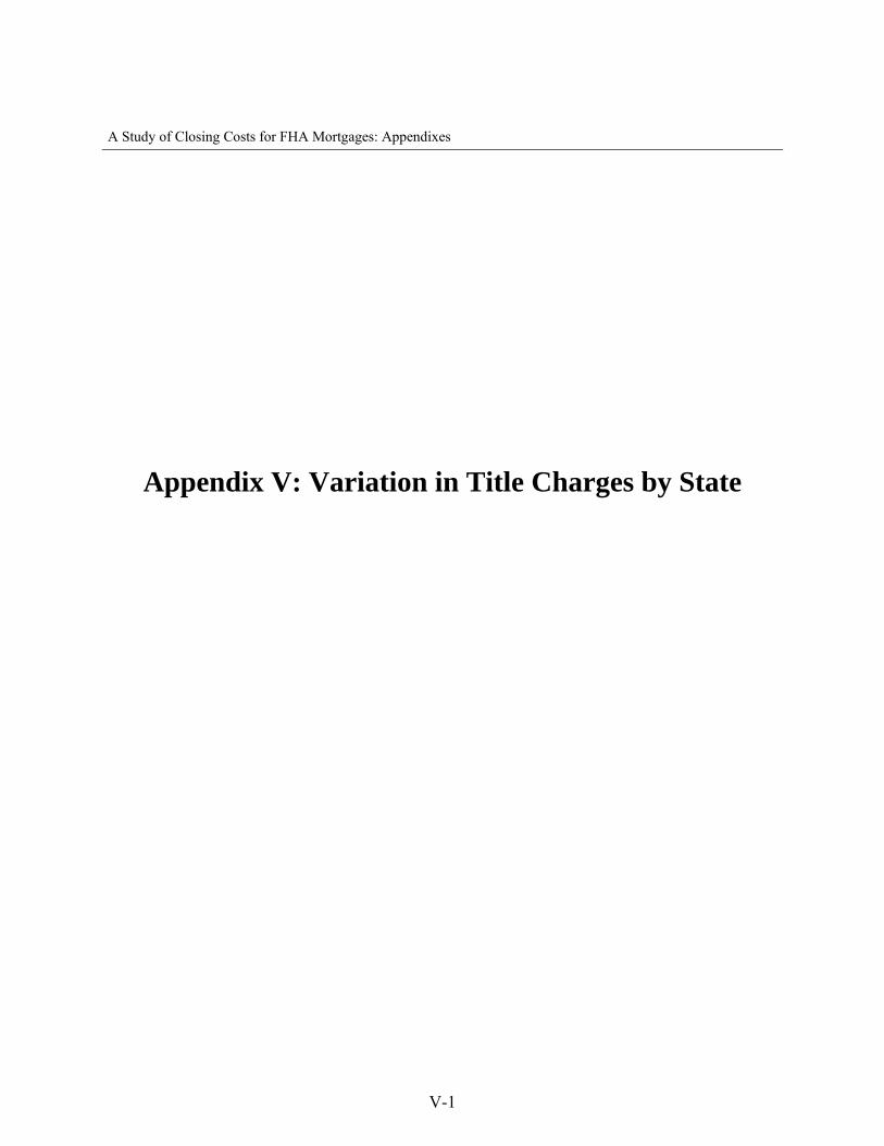
A Study of Closing Costs for FHA Mortgages: Appendixes
Appendix V: Variation in Title Charges by State
V-1
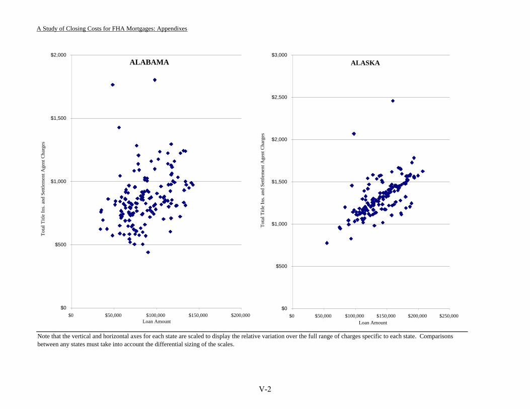
A Study of Closing Costs for FHA Mortgages: Appendixes
Note that the vertical and horizontal axes for each state are scaled to display the relative variation over the full range of charges specific to each state. Comparisons between any states must take into account the differential sizing of the scales.
ALABAMA
$0
$500
$1,000
$1,500
$2,000
$0 $50,000 $100,000 $150,000 $200,000Loan Amount
Tota
l Titl
e In
s. an
d Se
ttlem
ent A
gent
Cha
rges
ALASKA
$0
$500
$1,000
$1,500
$2,000
$2,500
$3,000
$0 $50,000 $100,000 $150,000 $200,000 $250,000Loan Amount
Tota
l Titl
e In
s. an
d Se
ttlem
ent A
gent
Cha
rges
V-2

A Study of Closing Costs for FHA Mortgages: Appendixes
Note that the vertical and horizontal axes for each state are scaled to display the relative variation over the full range of charges specific to each state. Comparisons between any states must take into account the differential sizing of the scales.
ARIZONA
$0
$500
$1,000
$1,500
$2,000
$2,500
$0 $50,000 $100,000 $150,000 $200,000Loan Amount
Tota
l Titl
e In
s. an
d Se
ttlem
ent A
gent
Cha
rges
ARKANSAS
$0
$500
$1,000
$1,500
$2,000
$2,500
$3,000
$0 $50,000 $100,000 $150,000 $200,000Loan Amount
Tota
l Titl
e In
s. an
d Se
ttlem
ent A
gent
Cha
rges
V-3
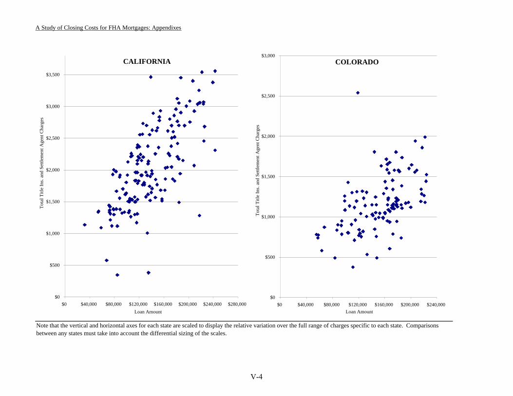
A Study of Closing Costs for FHA Mortgages: Appendixes
Note that the vertical and horizontal axes for each state are scaled to display the relative variation over the full range of charges specific to each state. Comparisons between any states must take into account the differential sizing of the scales.
CALIFORNIA
$0
$500
$1,000
$1,500
$2,000
$2,500
$3,000
$3,500
$0 $40,000 $80,000 $120,000 $160,000 $200,000 $240,000 $280,000Loan Amount
Tota
l Titl
e In
s. an
d Se
ttlem
ent A
gent
Cha
rges
COLORADO
$0
$500
$1,000
$1,500
$2,000
$2,500
$3,000
$0 $40,000 $80,000 $120,000 $160,000 $200,000 $240,000Loan Amount
Tota
l Titl
e In
s. an
d Se
ttlem
ent A
gent
Cha
rges
V-4
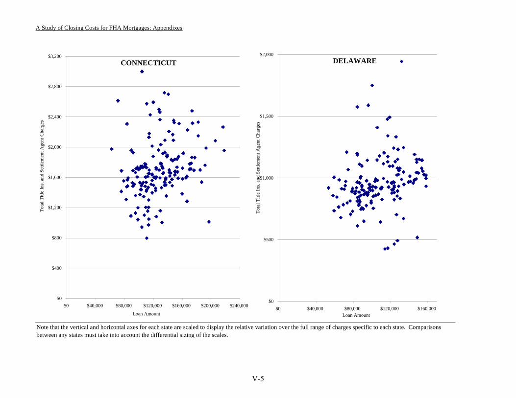
A Study of Closing Costs for FHA Mortgages: Appendixes
Note that the vertical and horizontal axes for each state are scaled to display the relative variation over the full range of charges specific to each state. Comparisons between any states must take into account the differential sizing of the scales.
CONNECTICUT
$0
$400
$800
$1,200
$1,600
$2,000
$2,400
$2,800
$3,200
$0 $40,000 $80,000 $120,000 $160,000 $200,000 $240,000
Loan Amount
Tota
l Titl
e In
s. an
d Se
ttlem
ent A
gent
Cha
rges
DELAWARE
$0
$500
$1,000
$1,500
$2,000
$0 $40,000 $80,000 $120,000 $160,000Loan Amount
Tota
l Titl
e In
s. an
d Se
ttlem
ent A
gent
Cha
rges
V-5
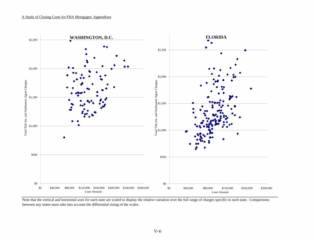
A Study of Closing Costs for FHA Mortgages: Appendixes
Note that the vertical and horizontal axes for each state are scaled to display the relative variation over the full range of charges specific to each state. Comparisons between any states must take into account the differential sizing of the scales.
WASHINGTON, D.C.
$0
$500
$1,000
$1,500
$2,000
$2,500
$0 $40,000 $80,000 $120,000 $160,000 $200,000 $240,000 $280,000Loan Amount
Tota
l Titl
e In
s. an
d Se
ttlem
ent A
gent
Cha
rges
FLORIDA
$0
$500
$1,000
$1,500
$2,000
$2,500
$0 $40,000 $80,000 $120,000 $160,000 $200,000Loan Amount
Tota
l Titl
e In
s. an
d Se
ttlem
ent A
gent
Cha
rges
V-6
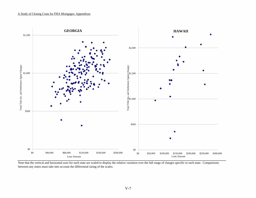
A Study of Closing Costs for FHA Mortgages: Appendixes
Note that the vertical and horizontal axes for each state are scaled to display the relative variation over the full range of charges specific to each state. Comparisons between any states must take into account the differential sizing of the scales.
GEORGIA
$0
$500
$1,000
$1,500
$0 $40,000 $80,000 $120,000 $160,000 $200,000Loan Amount
Tota
l Titl
e In
s. an
d Se
ttlem
ent A
gent
Cha
rges
HAWAII
$0
$500
$1,000
$1,500
$2,000
$0 $50,000 $100,000 $150,000 $200,000 $250,000 $300,000Loan Amount
Tota
l Titl
e In
s. an
d Se
ttlem
ent A
gent
Cha
rges
V-7
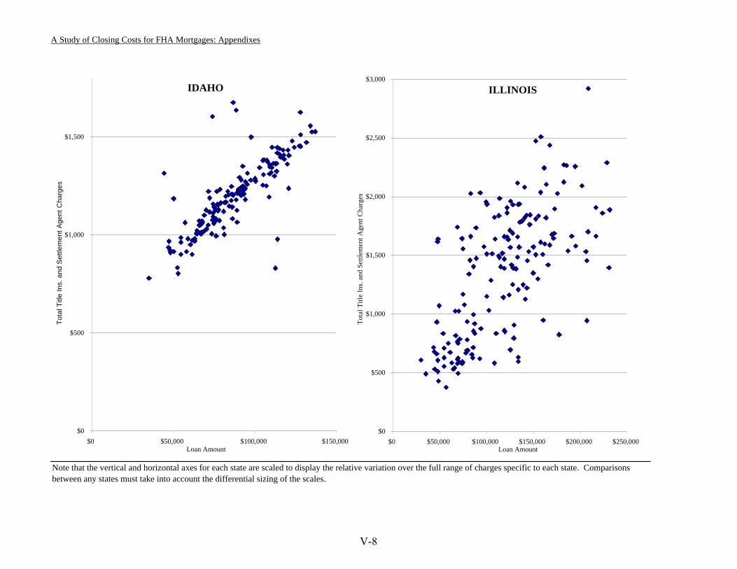
A Study of Closing Costs for FHA Mortgages: Appendixes
Note that the vertical and horizontal axes for each state are scaled to display the relative variation over the full range of charges specific to each state. Comparisons between any states must take into account the differential sizing of the scales.
IDAHO
$0
$500
$1,000
$1,500
$0 $50,000 $100,000 $150,000Loan Amount
Tota
l Titl
e In
s. a
nd S
ettle
men
t Age
nt C
harg
es
ILLINOIS
$0
$500
$1,000
$1,500
$2,000
$2,500
$3,000
$0 $50,000 $100,000 $150,000 $200,000 $250,000Loan Amount
Tota
l Titl
e In
s. an
d Se
ttlem
ent A
gent
Cha
rges
V-8
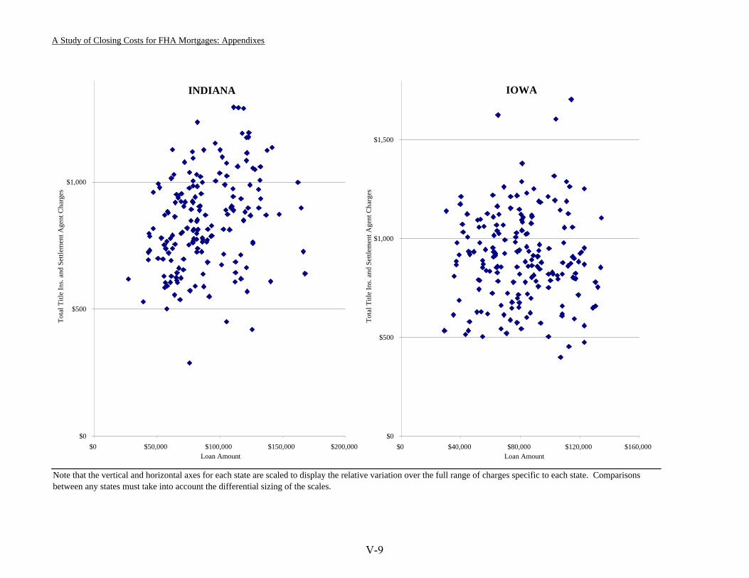
A Study of Closing Costs for FHA Mortgages: Appendixes
Note that the vertical and horizontal axes for each state are scaled to display the relative variation over the full range of charges specific to each state. Comparisons between any states must take into account the differential sizing of the scales.
INDIANA
$0
$500
$1,000
$0 $50,000 $100,000 $150,000 $200,000Loan Amount
Tota
l Titl
e In
s. an
d Se
ttlem
ent A
gent
Cha
rges
IOWA
$0
$500
$1,000
$1,500
$0 $40,000 $80,000 $120,000 $160,000Loan Amount
Tota
l Titl
e In
s. an
d Se
ttlem
ent A
gent
Cha
rges
V-9
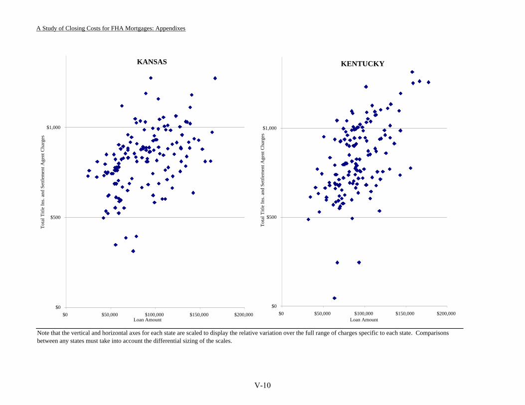
A Study of Closing Costs for FHA Mortgages: Appendixes
Note that the vertical and horizontal axes for each state are scaled to display the relative variation over the full range of charges specific to each state. Comparisons between any states must take into account the differential sizing of the scales.
KANSAS
$0
$500
$1,000
$0 $50,000 $100,000 $150,000 $200,000Loan Amount
Tota
l Titl
e In
s. an
d Se
ttlem
ent A
gent
Cha
rges
KENTUCKY
$0
$500
$1,000
$0 $50,000 $100,000 $150,000 $200,000Loan Amount
Tota
l Titl
e In
s. an
d Se
ttlem
ent A
gent
Cha
rges
V-10
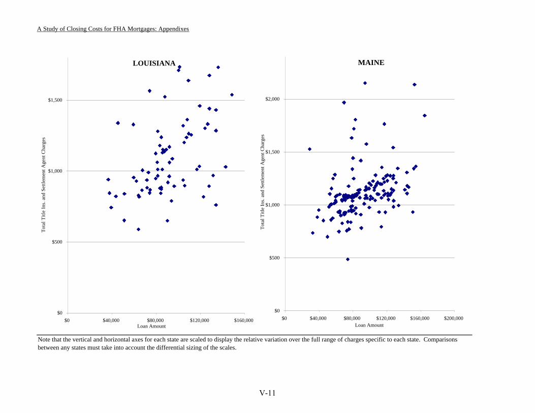
A Study of Closing Costs for FHA Mortgages: Appendixes
Note that the vertical and horizontal axes for each state are scaled to display the relative variation over the full range of charges specific to each state. Comparisons between any states must take into account the differential sizing of the scales.
LOUISIANA
$0
$500
$1,000
$1,500
$0 $40,000 $80,000 $120,000 $160,000Loan Amount
Tota
l Titl
e In
s. an
d Se
ttlem
ent A
gent
Cha
rges
MAINE
$0
$500
$1,000
$1,500
$2,000
$0 $40,000 $80,000 $120,000 $160,000 $200,000Loan Amount
Tota
l Titl
e In
s. an
d Se
ttlem
ent A
gent
Cha
rges
V-11
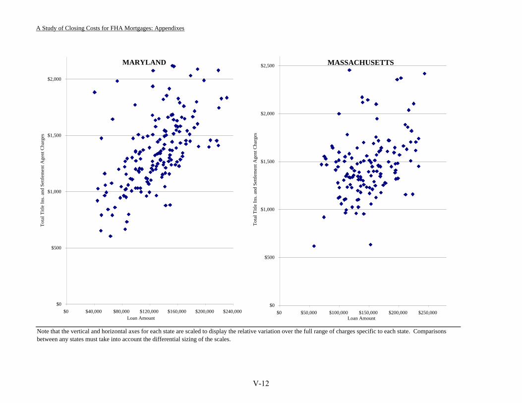
A Study of Closing Costs for FHA Mortgages: Appendixes
Note that the vertical and horizontal axes for each state are scaled to display the relative variation over the full range of charges specific to each state. Comparisons between any states must take into account the differential sizing of the scales.
MARYLAND
$0
$500
$1,000
$1,500
$2,000
$0 $40,000 $80,000 $120,000 $160,000 $200,000 $240,000Loan Amount
Tota
l Titl
e In
s. an
d Se
ttlem
ent A
gent
Cha
rges
MASSACHUSETTS
$0
$500
$1,000
$1,500
$2,000
$2,500
$0 $50,000 $100,000 $150,000 $200,000 $250,000Loan Amount
Tota
l Titl
e In
s. an
d Se
ttlem
ent A
gent
Cha
rges
V-12
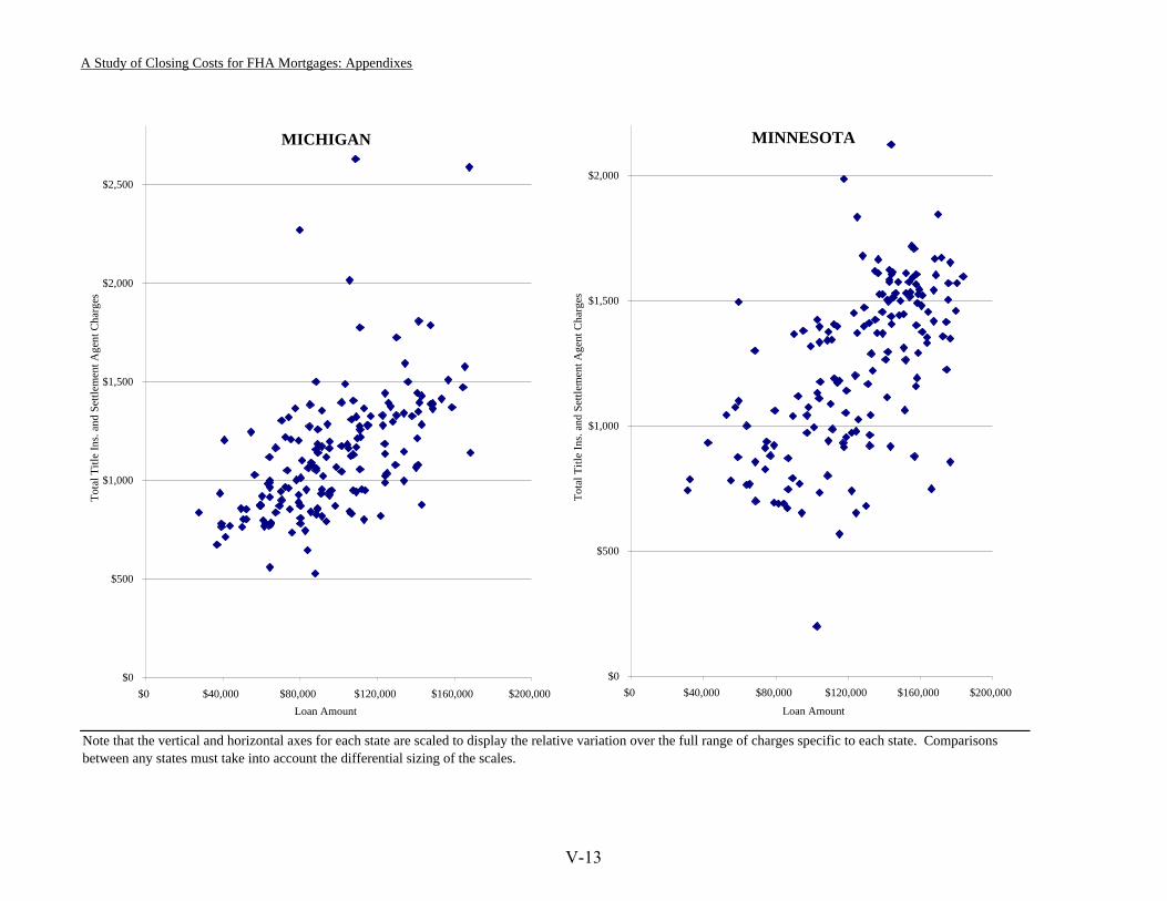
A Study of Closing Costs for FHA Mortgages: Appendixes
Note that the vertical and horizontal axes for each state are scaled to display the relative variation over the full range of charges specific to each state. Comparisons between any states must take into account the differential sizing of the scales.
MICHIGAN
$0
$500
$1,000
$1,500
$2,000
$2,500
$0 $40,000 $80,000 $120,000 $160,000 $200,000Loan Amount
Tota
l Titl
e In
s. an
d Se
ttlem
ent A
gent
Cha
rges
MINNESOTA
$0
$500
$1,000
$1,500
$2,000
$0 $40,000 $80,000 $120,000 $160,000 $200,000
Loan Amount
Tota
l Titl
e In
s. an
d Se
ttlem
ent A
gent
Cha
rges
V-13
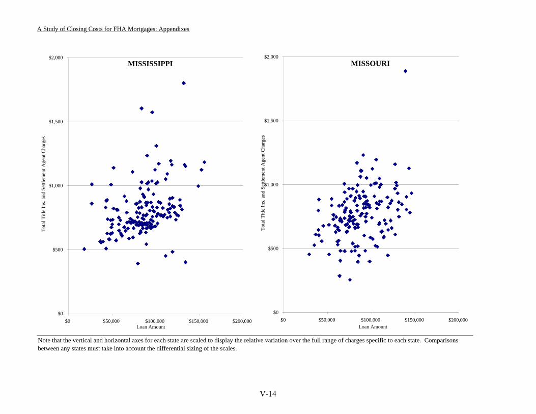
A Study of Closing Costs for FHA Mortgages: Appendixes
Note that the vertical and horizontal axes for each state are scaled to display the relative variation over the full range of charges specific to each state. Comparisons between any states must take into account the differential sizing of the scales.
MISSISSIPPI
$0
$500
$1,000
$1,500
$2,000
$0 $50,000 $100,000 $150,000 $200,000Loan Amount
Tota
l Titl
e In
s. an
d Se
ttlem
ent A
gent
Cha
rges
MISSOURI
$0
$500
$1,000
$1,500
$2,000
$0 $50,000 $100,000 $150,000 $200,000Loan Amount
Tota
l Titl
e In
s. an
d Se
ttlem
ent A
gent
Cha
rges
V-14
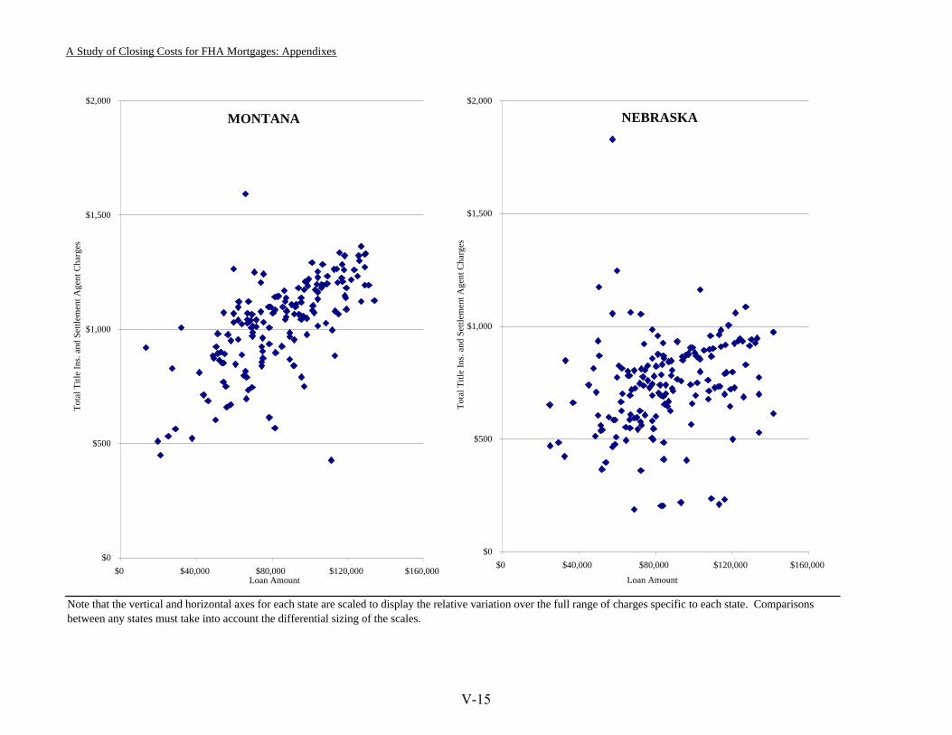
A Study of Closing Costs for FHA Mortgages: Appendixes
Note that the vertical and horizontal axes for each state are scaled to display the relative variation over the full range of charges specific to each state. Comparisons between any states must take into account the differential sizing of the scales.
MONTANA
$0
$500
$1,000
$1,500
$2,000
$0 $40,000 $80,000 $120,000 $160,000Loan Amount
Tota
l Titl
e In
s. an
d Se
ttlem
ent A
gent
Cha
rges
NEBRASKA
$0
$500
$1,000
$1,500
$2,000
$0 $40,000 $80,000 $120,000 $160,000
Loan Amount
Tota
l Titl
e In
s. an
d Se
ttlem
ent A
gent
Cha
rges
V-15
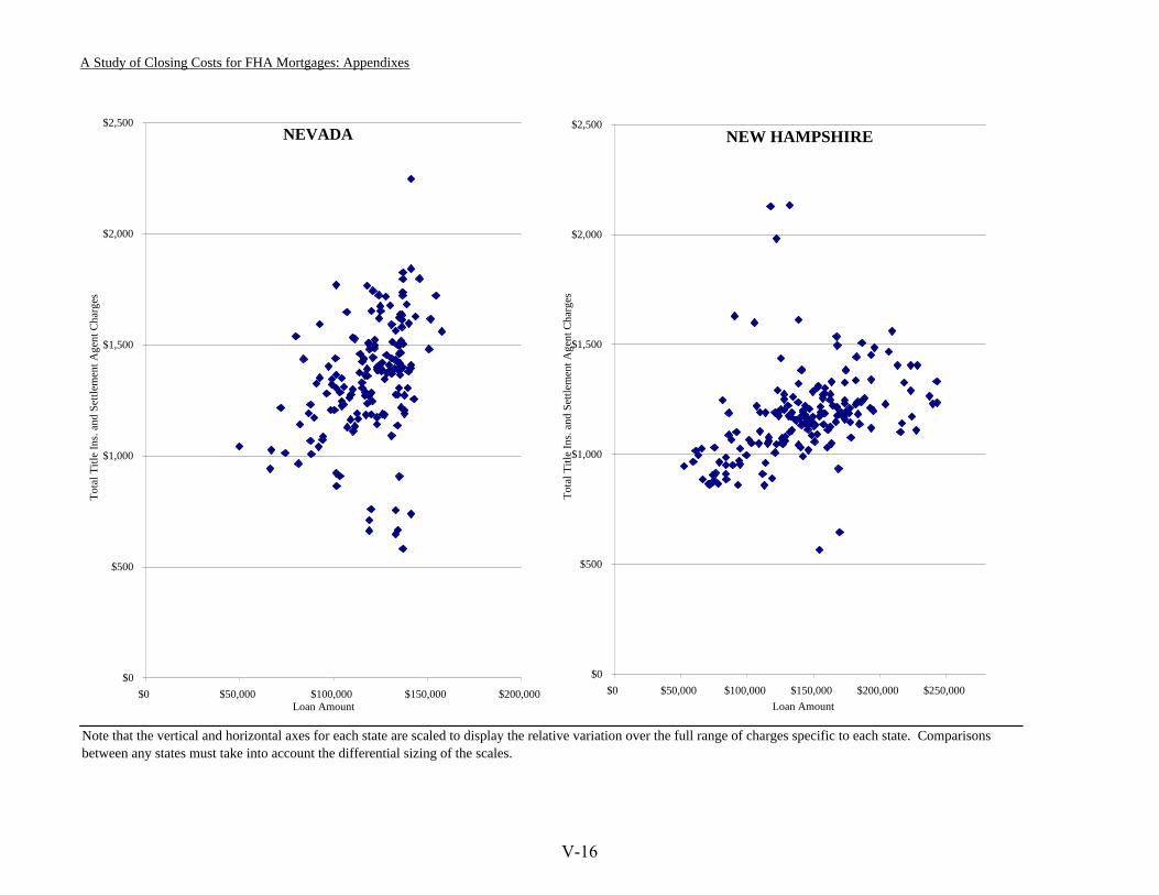
A Study of Closing Costs for FHA Mortgages: Appendixes
Note that the vertical and horizontal axes for each state are scaled to display the relative variation over the full range of charges specific to each state. Comparisons between any states must take into account the differential sizing of the scales.
NEVADA
$0
$500
$1,000
$1,500
$2,000
$2,500
$0 $50,000 $100,000 $150,000 $200,000Loan Amount
Tota
l Titl
e In
s. an
d Se
ttlem
ent A
gent
Cha
rges
NEW HAMPSHIRE
$0
$500
$1,000
$1,500
$2,000
$2,500
$0 $50,000 $100,000 $150,000 $200,000 $250,000Loan Amount
Tota
l Titl
e In
s. an
d Se
ttlem
ent A
gent
Cha
rges
V-16
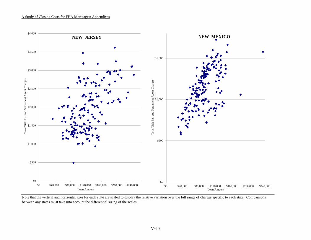
A Study of Closing Costs for FHA Mortgages: Appendixes
Note that the vertical and horizontal axes for each state are scaled to display the relative variation over the full range of charges specific to each state. Comparisons between any states must take into account the differential sizing of the scales.
NEW JERSEY
$0
$500
$1,000
$1,500
$2,000
$2,500
$3,000
$3,500
$4,000
$0 $40,000 $80,000 $120,000 $160,000 $200,000 $240,000Loan Amount
Tota
l Titl
e In
s. an
d Se
ttlem
ent A
gent
Cha
rges
NEW MEXICO
$0
$500
$1,000
$1,500
$0 $40,000 $80,000 $120,000 $160,000 $200,000 $240,000Loan Amount
Tota
l Titl
e In
s. an
d Se
ttlem
ent A
gent
Cha
rges
V-17
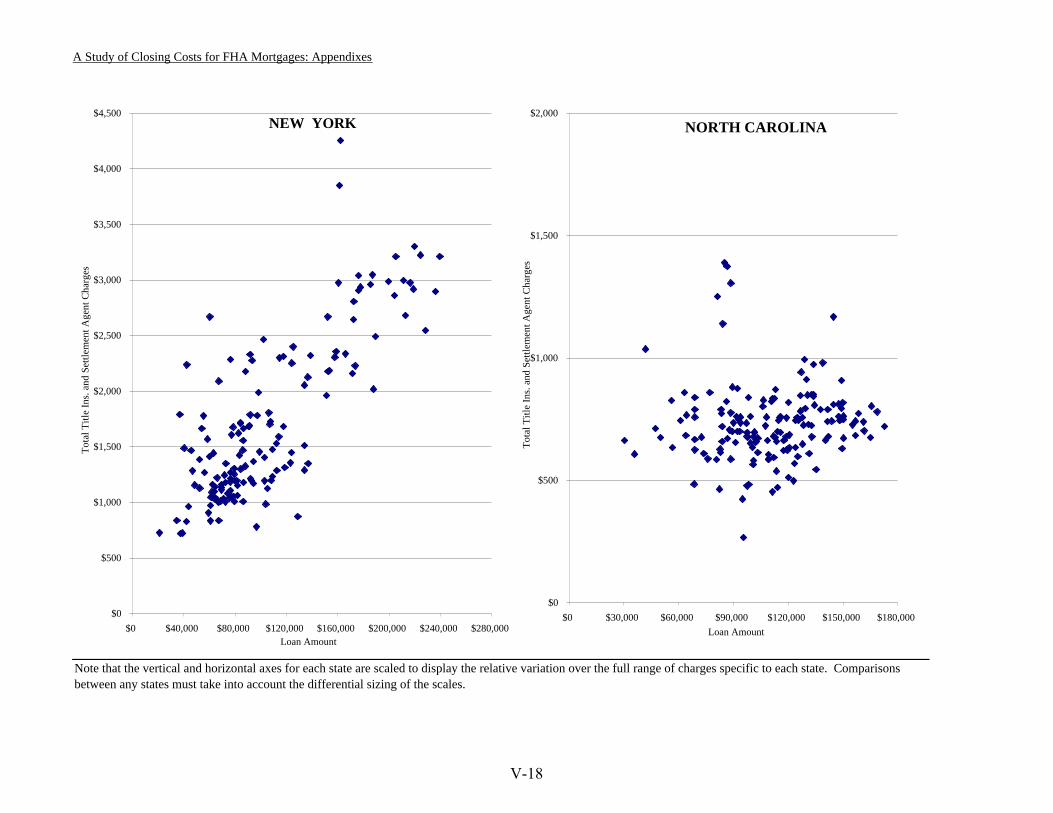
A Study of Closing Costs for FHA Mortgages: Appendixes
Note that the vertical and horizontal axes for each state are scaled to display the relative variation over the full range of charges specific to each state. Comparisons between any states must take into account the differential sizing of the scales.
NEW YORK
$0
$500
$1,000
$1,500
$2,000
$2,500
$3,000
$3,500
$4,000
$4,500
$0 $40,000 $80,000 $120,000 $160,000 $200,000 $240,000 $280,000Loan Amount
Tota
l Titl
e In
s. an
d Se
ttlem
ent A
gent
Cha
rges
NORTH CAROLINA
$0
$500
$1,000
$1,500
$2,000
$0 $30,000 $60,000 $90,000 $120,000 $150,000 $180,000Loan Amount
Tota
l Titl
e In
s. an
d Se
ttlem
ent A
gent
Cha
rges
V-18
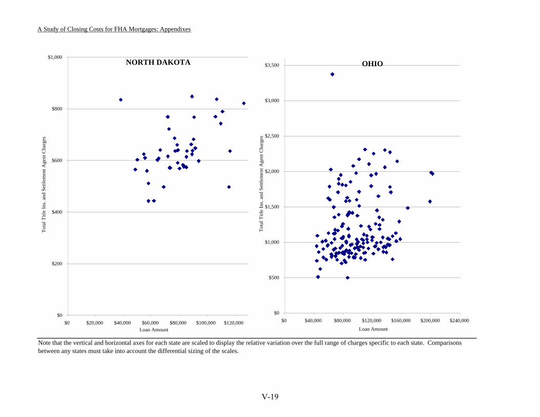
A Study of Closing Costs for FHA Mortgages: Appendixes
Note that the vertical and horizontal axes for each state are scaled to display the relative variation over the full range of charges specific to each state. Comparisons between any states must take into account the differential sizing of the scales.
NORTH DAKOTA
$0
$200
$400
$600
$800
$1,000
$0 $20,000 $40,000 $60,000 $80,000 $100,000 $120,000Loan Amount
Tota
l Titl
e In
s. an
d Se
ttlem
ent A
gent
Cha
rges
OHIO
$0
$500
$1,000
$1,500
$2,000
$2,500
$3,000
$3,500
$0 $40,000 $80,000 $120,000 $160,000 $200,000 $240,000
Loan Amount
Tota
l Titl
e In
s. an
d Se
ttlem
ent A
gent
Cha
rges
V-19
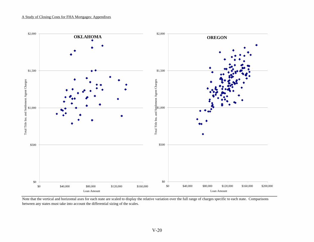
A Study of Closing Costs for FHA Mortgages: Appendixes
Note that the vertical and horizontal axes for each state are scaled to display the relative variation over the full range of charges specific to each state. Comparisons between any states must take into account the differential sizing of the scales.
OKLAHOMA
$0
$500
$1,000
$1,500
$2,000
$0 $40,000 $80,000 $120,000 $160,000Loan Amount
Tota
l Titl
e In
s. an
d Se
ttlem
ent A
gent
Cha
rges
OREGON
$0
$500
$1,000
$1,500
$2,000
$0 $40,000 $80,000 $120,000 $160,000 $200,000
Loan Amount
Tota
l Titl
e In
s. an
d Se
ttlem
ent A
gent
Cha
rges
V-20
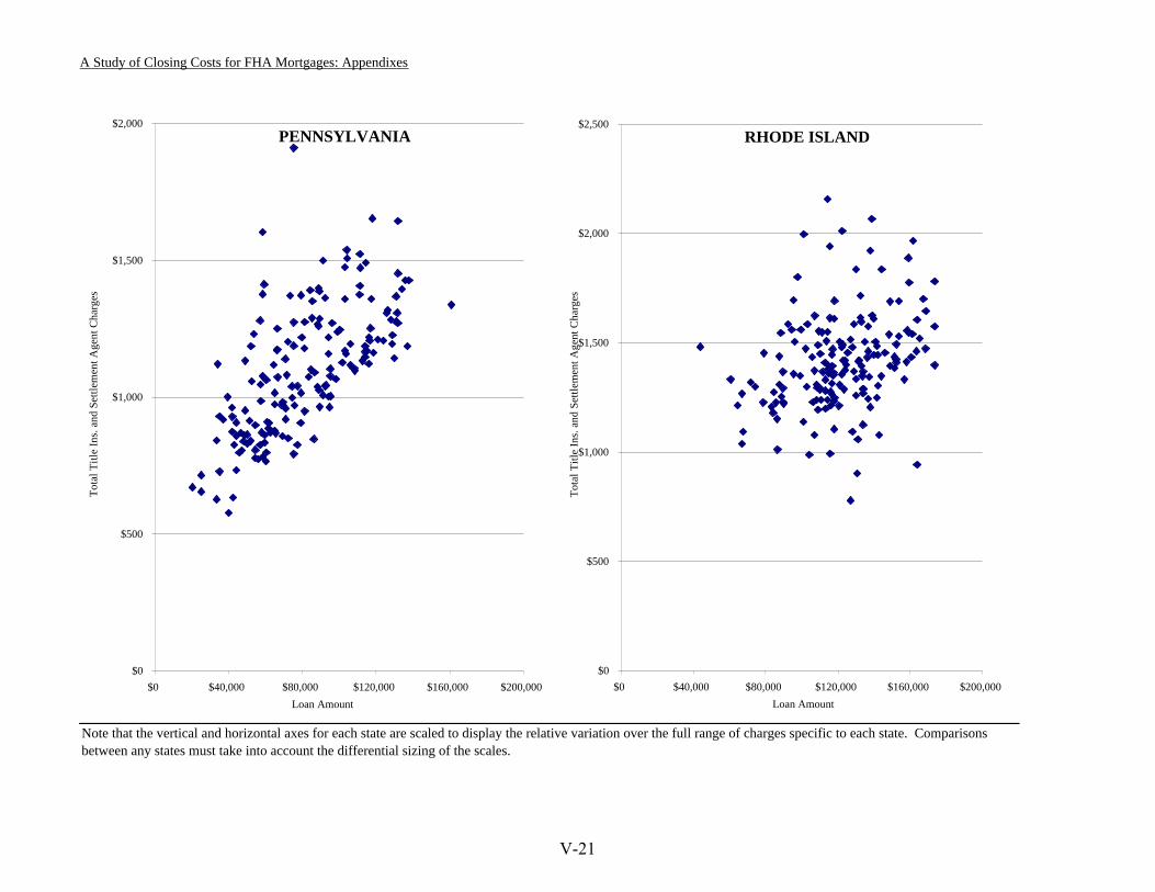
A Study of Closing Costs for FHA Mortgages: Appendixes
Note that the vertical and horizontal axes for each state are scaled to display the relative variation over the full range of charges specific to each state. Comparisons between any states must take into account the differential sizing of the scales.
PENNSYLVANIA
$0
$500
$1,000
$1,500
$2,000
$0 $40,000 $80,000 $120,000 $160,000 $200,000Loan Amount
Tota
l Titl
e In
s. an
d Se
ttlem
ent A
gent
Cha
rges
RHODE ISLAND
$0
$500
$1,000
$1,500
$2,000
$2,500
$0 $40,000 $80,000 $120,000 $160,000 $200,000Loan Amount
Tota
l Titl
e In
s. an
d Se
ttlem
ent A
gent
Cha
rges
V-21
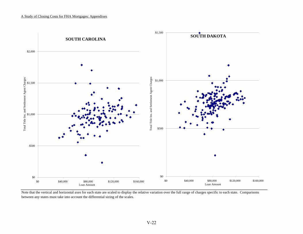
A Study of Closing Costs for FHA Mortgages: Appendixes
Note that the vertical and horizontal axes for each state are scaled to display the relative variation over the full range of charges specific to each state. Comparisons between any states must take into account the differential sizing of the scales.
SOUTH CAROLINA
$0
$500
$1,000
$1,500
$2,000
$0 $40,000 $80,000 $120,000 $160,000Loan Amount
Tota
l Titl
e In
s. an
d Se
ttlem
ent A
gent
Cha
rges
SOUTH DAKOTA
$0
$500
$1,000
$1,500
$0 $40,000 $80,000 $120,000 $160,000Loan Amount
Tota
l Titl
e In
s. an
d Se
ttlem
ent A
gent
Cha
rges
V-22
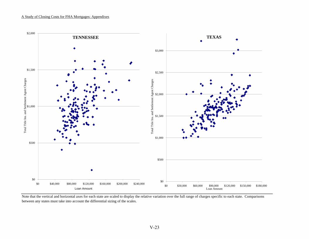
A Study of Closing Costs for FHA Mortgages: Appendixes
Note that the vertical and horizontal axes for each state are scaled to display the relative variation over the full range of charges specific to each state. Comparisons between any states must take into account the differential sizing of the scales.
TENNESSEE
$0
$500
$1,000
$1,500
$2,000
$0 $40,000 $80,000 $120,000 $160,000 $200,000 $240,000Loan Amount
Tota
l Titl
e In
s. an
d Se
ttlem
ent A
gent
Cha
rges
TEXAS
$0
$500
$1,000
$1,500
$2,000
$2,500
$3,000
$0 $30,000 $60,000 $90,000 $120,000 $150,000 $180,000Loan Amount
Tota
l Titl
e In
s. an
d Se
ttlem
ent A
gent
Cha
rges
V-23
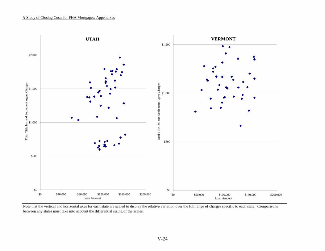
A Study of Closing Costs for FHA Mortgages: Appendixes
Note that the vertical and horizontal axes for each state are scaled to display the relative variation over the full range of charges specific to each state. Comparisons between any states must take into account the differential sizing of the scales.
UTAH
$0
$500
$1,000
$1,500
$2,000
$0 $40,000 $80,000 $120,000 $160,000 $200,000Loan Amount
Tota
l Titl
e In
s. an
d Se
ttlem
ent A
gent
Cha
rges
VERMONT
$0
$500
$1,000
$1,500
$0 $50,000 $100,000 $150,000 $200,000Loan Amount
Tota
l Titl
e In
s. an
d Se
ttlem
ent A
gent
Cha
rges
V-24
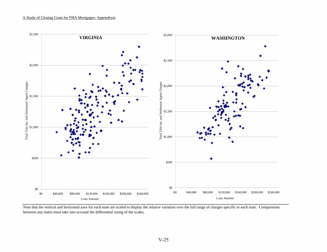
A Study of Closing Costs for FHA Mortgages: Appendixes
Note that the vertical and horizontal axes for each state are scaled to display the relative variation over the full range of charges specific to each state. Comparisons between any states must take into account the differential sizing of the scales.
VIRGINIA
$0
$500
$1,000
$1,500
$2,000
$2,500
$0 $40,000 $80,000 $120,000 $160,000 $200,000 $240,000
Loan Amount
Tota
l Titl
e In
s. an
d Se
ttlem
ent A
gent
Cha
rges
WASHINGTON
$0
$500
$1,000
$1,500
$2,000
$2,500
$3,000
$0 $40,000 $80,000 $120,000 $160,000 $200,000 $240,000
Loan Amount
Tota
l Titl
e In
s. an
d Se
ttlem
ent A
gent
Cha
rges
V-25
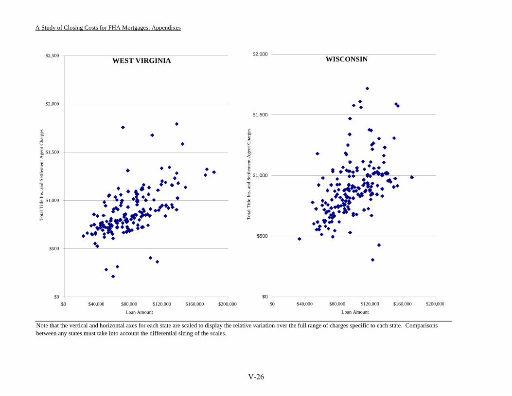
A Study of Closing Costs for FHA Mortgages: Appendixes
Note that the vertical and horizontal axes for each state are scaled to display the relative variation over the full range of charges specific to each state. Comparisons between any states must take into account the differential sizing of the scales.
WEST VIRGINIA
$0
$500
$1,000
$1,500
$2,000
$2,500
$0 $40,000 $80,000 $120,000 $160,000 $200,000
Loan Amount
Tota
l Titl
e In
s. an
d Se
ttlem
ent A
gent
Cha
rges
WISCONSIN
$0
$500
$1,000
$1,500
$2,000
$0 $40,000 $80,000 $120,000 $160,000 $200,000
Loan Amount
Tota
l Titl
e In
s. an
d Se
ttlem
ent A
gent
Cha
rges
V-26
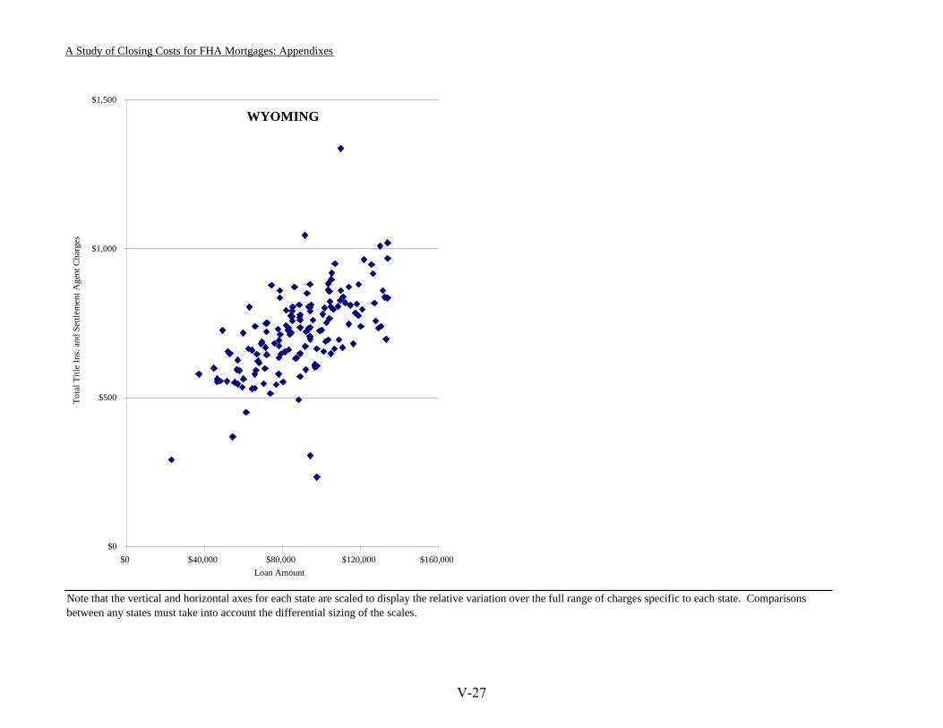
A Study of Closing Costs for FHA Mortgages: Appendixes
Note that the vertical and horizontal axes for each state are scaled to display the relative variation over the full range of charges specific to each state. Comparisons between any states must take into account the differential sizing of the scales.
WYOMING
$0
$500
$1,000
$1,500
$0 $40,000 $80,000 $120,000 $160,000Loan Amount
Tota
l Titl
e In
s. an
d Se
ttlem
ent A
gent
Cha
rges
V-27
A Study of Closing Costs for FHA Mortgages: Appendixes
Notes Chapter I 1. Important exceptions are the studies by the Federal Trade Commission (Lacko and Pappalardo 2007) and by HUD. 2. For RESPA purposes, HUD defines a mortgage broker as a person or firm that originates loans in the name of a lender but never holds titles to the loans. Such a transaction is generally referred to as a “table funded” loan. It is a transaction-specific, rather than occupation- or firm-specific, definition. A person or firm may be a HUD-defined broker in one transaction but not in another. 3. Sometimes, especially for larger principal balance loans for which the 1/8 tick in which mortgage interest rates are quoted is constraining, the borrower will get a check at closing for the excess of the YSP over the closing costs.
4. When mortgages began to be securitized, it was necessary to organize arrangements to ensure that the booking of payments and monitoring of borrowers (and pursuance of foreclosure if necessary) continued after a lender sold the note into the secondary market. This is arranged by paying a portion of the interest to the mortgage servicer who performs these functions. This interest rate strip (44 basis points for GNMA, 25 basis points for Freddie Mac and Fannie Mae) is more than it costs on average to service loans. Thus, servicers bid for the right to receive the interest strip and perform the servicing. With their investment as a hostage to exchange (to be lost if the guarantor forces a transfer of servicing in the case of GNMA), the servicer has incentive to keep the loan current and performing. Servicing on new loans typically sells in the range of 1 to 1.5 percent of the principal amount of the loan and is a function of average loan amount, credit quality, and prepayment speed. 5. All ARMs have both annual and life-of-loan caps, by federal law, partly as a result of the Truth in Lending Act requirement that lenders disclose the total number of dollars that could ever have to be repaid on the loan. Without caps, the possible total is unlimited. 6. The value of the option to prepay and the separating equilibrium are discussed in Stanton and Wallace (1998) and Brueckner (1994). See references.
Chapter V 1. Variables that affect loan pricing due to their influence on default probability are interacted with loan amount because losses from default increase with loan amount.
Chapter VI 1. “Points” have been the subject of some hand-wringing at FHA. Before 1983, the FHA commissioner set ceilings on the rate and points allowed on FHA loans but evidently did not adjust them often enough to reflect market conditions. When interest rates bumped up against the FHA ceilings, sellers started paying points for buyers (presumably in exchange for a higher price on the house) and even real estate agents started paying points (presumably in exchange for a higher fee) in order to get transactions completed. Thus, the term “points” has meant many different things in different situations, providing further reason for borrowers to be confused. Though 1983 may seem a long time ago, it is not in the evolution of markets and their practices. The original interest rate on a bond or a mortgage is called a “coupon” rate even though it has been decades since any bonds had coupons to be torn off (along perforations), submitted, and redeemed for interest payments.
A Study of Closing Costs for FHA Mortgages: Appendixes
2. Analysis by Asabere and Hoffman (1997) finds that house prices in the conventional market, but not the FHA market, are inflated by seller contributions.
Chapter VIII 1. There is no instrument available for a measurement using instrumental variables.
Chapter IX 1. George Stigler originated this phrase.
Chapter X 1. See Birnbaum (2005) as well as the 10K filings with the SEC for the largest title insurers. 2. See http://www.legaldeeds.com/Interface/Services/Conveyances/Canada/BC/real_estate_title_search/ questionnaire.php?affiliate_id=enroute.
Appendix IV 1. Lipshutz (1994, 1) states: “Title insurance is unique in that it is insurance against ignorance of the past, that is, whether some unknown past event has clouded the ownership interest or lien interest in a parcel of real property that the insured believes to exist when the title insurance policy is issued.” 2. The 2006 GAO report notes that “the amount of premium paid to or retained by title agents, generally to pay for title search and examination costs and agents’ commissions, accounted for approximately 71 percent of title insurers’ total premiums written in 2004” (p. 3). 3. In fact, GAO (2007) reports that title insurers themselves do little analysis of actual costs incurred by agents and that the percentage of premium retained by agents was negotiated based on various factors but not generally the agent’s actual costs. 4. Holden Lewis, “Study reveals closing cost differences,” Bankrate.com, http://www.bankrate.com/brm/news/mortgages/ccmain.asp, accessed May 4, 2006. 5. Lewis attributes this explanation to James Maher, executive vice president of ALTA. Indicative of a lack of cost basis for title insurance rates is the discussion in GAO (2007, 39) reporting that insurers “generally share the same percentage of the premium with their agents, around 80 to 90 percent, regardless of whether those agents were in states where consumers were to pay for agents’ search and examination services within the premium rate … or whether they were in states where agents can charge consumers separately for these services.” 6. Lipshutz (1994) estimates the average agent commission as 80 percent. 7. Lipshutz (1994, 50) agrees this pricing pattern results in a cross-subsidization for small consumers (as “cost per transaction was not strongly dependent on the amount of liability insured”). Birnbaum (2005, 22) notes that (for California at least) “like title insurance rates, escrow fees vary by the size of the transaction. Unlike title insurance rates, escrow fees also vary by county.” 8. Woodward (2003), however, in an econometric study of the determinants of title insurance fees, fails to find this relationship; while these fees increase with loan value, the effect is not statistically significant once other factors —in particular yield spread premiums on the loan—are included. This puzzling result deserves further exploration,
A Study of Closing Costs for FHA Mortgages: Appendixes
considering that the monotonic relationship between title fees and loan size is accepted as truth by virtually all who have written on the industry. 9. Kenneth R. Harney, “Refinancing’s Magic Words: Reissue Rate,” Washington Post, June 8, 2002, p. H1. Harney quotes James R. Maher, executive vice president of ALTA acknowledging that the association is “aware that not all of our members disclose” the possibility of these reissue discounts. 10. Erin Toll, a deputy commissioner at the Colorado Division of Insurance, testified before the House Financial Services Subcommittee on Housing and Community Opportunity on April 26, 20006 that “there is no financial necessity to reinsure in a residential, single-family dwelling—there’s absolutely none.” 11. Washington Post, “Title Insurers Settle With N.Y.,” May 24, 2006, p. D-2. 12. For example, Vistnes (2006), critiquing the study on behalf of the California Land Title Association, rejects the analyses in the Birnbaum report. 13. GAO (2007) provides similar figures for 2005 and points out that concentration is even higher than this in individual states, with two or three insurers generally dominant. 14. Nyce and Boyer (1998, 228) posit that requiring title plants may be a barrier to entry. They present some data suggesting that in the 15 states not requiring title plants, there are more title insurers and a lower Herfindahl index (a measure of market concentration)—even after controlling for differences in state size. Nyce and Boyer do, however, expect that technology will lessen this barrier. 15. Jaffee (2006) suggests there may be efficiencies associated with the monoline insurance requirement. 16. Nyce and Boyer (1998, 230–31) agree that controlled business arrangements may discourage new entry by requiring partnerships with existing producers of business (affiliations short of ownership raise the same issue). 17. In a similar vein, the 2006 GAO report (pp. 10–11) states that “while consumers are the ones paying for title insurance, they generally do not know how to ‘shop around’ for the best deal, and may not even know that they can. Meanwhile, the potential exists for real estate or mortgage professionals to recommend – not the least expensive or most reputable title insurer or agent – but the one that is most closely aligned with the professional’s best interest.” 18. See Stephen J. Quiner, “Title Insurance and the Title Insurance Industry,” 22 Drake L R. 711 (1973). 19. Average profitability was even higher for the other two holding companies over the same period, but a significant part of revenues for these companies was generated from non-title insurance sources. Stangle and Strombom (2006) make a different comparison—title company net income margin and operating profit margin versus property or casualty insurers, homebuilders, and the S&P 500—to claim title insurers have comparable or lower profits.


![Q2 2015 Mortgage Lender Sentiment Survey Questionnaire · /* Q10c */ Refinance - [* Government *] [- Government Mortgages primarily include Federal Housing Administration (FHA) and](https://img.pdfslide.net/doc/110x75/5f0972397e708231d426df3b/q2-2015-mortgage-lender-sentiment-survey-q10c-refinance-government-.jpg)