A STUDY OF CRACK-INCLUSION INTERACTION USING MOIRÉ

A STUDY OF CRACK-INCLUSION INTERACTION USING MOIRÉ

INTERFEROMETRY AND FINITE ELEMENT ANALYSIS

Except where reference is made to the work of others, the work described in this thesis is my own or was done in collaboration with my advisory committee. This thesis does not

include proprietary or classified information.

________________________________ Piyush Chunilal Savalia

Certificate of Approval:

______________________________ _____________________________ Jeffrey C. Suhling Hareesh V. Tippur, Chair Quina Distinguished Professor Alumni Professor Mechanical Engineering Mechanical Engineering ______________________________ _____________________________ Robert L. Jackson Stephen L. McFarland Assistant Professor Acting Dean Mechanical Engineering Graduate School



Piyush Chunilal Savalia

A Thesis

Submitted to

the Graduate Faculty of

Auburn University

in Partial Fulfillment of the

Requirements for the

Degree of

Master of Science

Auburn, Alabama December 15, 2006




Permission is granted to Auburn University to make copies of this thesis at its discretion upon request of individuals or institutions and at their expense. The author reserves all

publication rights.

_____________________________ Signature of Author

_____________________________

Date of Graduation

iii

VITA

Piyush Savalia, son of Chunilal and Kanchan Savalia, was born on December 13,

1979, in Gujarat, India. He earned a Bachelor’s degree in Mechanical Engineering from

Sardar Patel University, Vallabh Vidyanagar, India in 2002 with first class. After

Graduation he worked for Videocon Narmada Glass, a manufacturer of panels and

funnels for glass picture tubes in TV, in company’s captive power plant division as a

graduate engineer trainee. In August 2003, he began his graduate study in Mechanical

Engineering at Auburn University. He joined Dr. Hareesh V. Tippur’s research group in

January 2004, as a Graduate Research Assistant. He also worked as a Graduate Teaching

Assistant for the undergraduate course of Mechanics of Materials at Department of

Mechanical Engineering.

iv

THESIS ABSTRACT




Master of Science, December 15, 2006

(B. E., Sardar Patel University, Vallabh Vidyanagar, India, 2002)

131 Typed Pages

Directed by Hareesh V. Tippur

Failure of composite materials is intrinsically linked to the fundamental problem

of a matrix crack interacting with a second phase inclusion. In this work, the critical

issue of matrix-inclusion debonding in the presence of a nearby crack is addressed

experimentally and numerically. Optical measurement of surface deformations in the

vicinity of a crack-inclusion pair is carried out using moiré interferometry. The

measurements are used to validate an approach for simulating evolution of inclusion-

matrix debonding. The numerical model is subsequently used to parametrically study

crack-inclusion interactions.

In the first phase of this work, a process based on microlithography is developed

for creating master gratings on silicon wafers. Two methods are then developed to

transfer gratings to polymeric specimens. Edge cracked epoxy beams, each with a

v

cylindrical glass inclusion ahead of the crack tip, are fabricated to experimentally model

crack-inclusion interactions. A moiré interferometer for mapping displacement fields in

the crack-inclusion vicinity is developed. Debonding of an inclusion from the

surrounding matrix is detected successfully by the interferometer. The measured

displacements are analyzed to estimate surface strains and study the evolution of strain

fields associated with crack-inclusion debonding phenomenon. The associated effects on

fracture parameters namely, crack mouth opening displacements (CMOD), crack mouth

compliance, mode – I stress intensity factors (SIF) and energy release rates (ERR), are

extracted. A sharp rise in crack mouth compliance values and strains in the close vicinity

of the inclusion due to debonding is observed.

Next, a finite element model is developed to simulate the experimentally observed

behavior. Interfacial debonding between the matrix and the inclusion is simulated using

the element stiffness deactivation method. A failure criterion based on a critical radial

stress is shown to capture the onset and progression of debonding and finite element

results are in good agreement with measurements. A follow up parametric study is

performed to examine effects of inclusion size and inclusion proximity to the crack tip.

The results show that debonding is delayed as the inclusion size increases for a constant

L/d ratio where L and d are crack tip-inclusion distance and inclusion diameter,

respectively. For a constant L, debonding occurs at lower loads for larger inclusions

along with higher crack mouth compliance following inclusion-matrix debonding.

vi

ACKNOWLEDGEMENTS

I would like to thank my academic advisor, Dr. Hareesh V. Tippur for the

financial support and constant guidance throughout this work. Special thanks are due to

Madhusudhana Kirugulige, a doctoral candidate in our group and Charles Ellis, the lab

manager of Alabama Microelectronics Science and Technology Center (AMSTC), at

Auburn University’s Department of Electrical Engineering. Madhu’s help throughout my

stay at Auburn in many aspects is greatly appreciated. He introduced me to many

techniques and methods in the laboratory. His expertise and suggestions regarding the

finite element analysis issues were very helpful. This work would not have been possible

without cordial help by Charles. His suggestions and expertise in microelectronics

fabrication processes were of immense help. It was great to work with Dr. Rajesh Kitey,

a recent graduate and Taylor Owens, a master’s candidate in our group. Thanks are due

to my thesis committee members Dr. Jeff Suhling and Dr. Robert Jackson for reviewing

this work. I am very thankful to all my friends in Auburn and my cousin Dr. Jignesh

Dholaria for their constant support and for not letting me miss my family throughout my

stay at Auburn. I am indebted to my parents for their financial support and constant

moral support during my course of study at Auburn. Without their constant

encouragement and love it would not have been possible for me to do this work. I

dedicate this work to my parents.

vii

Style manual or journal used Discrete Mathematics (together with the style

known as “auphd”).

Computer software used The document preparation package Microsoft Word

2002 . SigmaPlot2001 was used for plotting the graphs.

viii

117

TABLE OF CONTENTS LIST OF FIGURES xi LIST OF TABLES xv

1. INTRODUCTION .......................................................................................................... 1

1.1 Composite materials: An overview........................................................................... 1

1.2 The crack-inclusion interaction problem .................................................................. 4

1.3 Background and literature survey ............................................................................. 6

1.4 Objectives ............................................................................................................... 10

1.5 Organization of the thesis ....................................................................................... 12 2. GRATINGS FABRICATION AND TRANSFER TECHNIQUES ............................. 13

2.1 Master gratings fabrication ..................................................................................... 15

2.2 Grating transfer methods......................................................................................... 21

2.2.1 Direct grating transfer from a silicon master ................................................... 21

2.2.2 Grating transfer using silicone rubber submasters........................................... 23

2.3 Crack-inclusion specimen fabrication..................................................................... 27 2.4 Materials characteristics.......................................................................................... 29 3. MOIRÉ INTERFEROMETRY..................................................................................... 32

3.1 Experimental Setup................................................................................................. 33

3.2 Deformation field mapping..................................................................................... 37 ix

118

3.3 Interference of plane waves .................................................................................... 37

3.4 In-plane moiré interferometry................................................................................. 40

3.5 Benchmark experiment ........................................................................................... 46 4. CRACK-INCLUSION INTERACTION...................................................................... 53

4.1 Interaction between crack and inclusion................................................................. 53

4.2 Fracture parameters and strains .............................................................................. 56

4.3 Experimental repeatability ...................................................................................... 61 5. FINITE ELEMENT MODELING................................................................................ 63

5.1 FEA model description ........................................................................................... 64

5.2 Inclusion-matrix debonding .................................................................................... 66

5.3 Effect of β on debonding ........................................................................................ 70

5.4 Convergence study.................................................................................................. 77

5.5 Parametric study...................................................................................................... 79

5.5.1 Constant L/d ratio: Effect of inclusion size...................................................... 79

5.5.2 Varying L/d ratio: Crack-inclusion proximity effect ....................................... 85

5.6 Estimation of glass-epoxy interface strength.......................................................... 90 6. CONCLUSIONS .......................................................................................................... 94 BIBLIOGRAPHY............................................................................................................. 97 APPENDICES ................................................................................................................ 100

A. ANSYS APDL Macros .......................................................................................... 101

B. Analysis of uncracked beam with inclusion........................................................... 114

x

118

LIST OF FIGURES

Figure 1.1 : Some applications of composite materials and relevance of the crack- inclusion interaction study. ............................................................................ 3 Figure 1.2 : Schematic of a matrix crack interacting with an inclusion. ........................... 5 Figure 2.1 : (a) LASI window showing mask design (b) Enlarged view of the gratings design in LASI (c) Mask (Ronchi gratings) made according to the design. 14 Figure 2.2 : (a) Wafer cleaning. (b) Dehydration bake.................................................... 15 Figure 2.3 : (a) HMDS application. (b) Photoresist application. ..................................... 17 Figure 2.4 : (a) Soft baking of the wafer. (b) The mask aligner showing the mask and The wafer. (Mask is held in the frame by vacuum.) .................................... 17 Figure 2.5 : (a) Photoresist development (b) Rinsing (c) Drying (d) Inspection under microscope. .................................................................................................. 18 Figure 2.6 : STS Multiplex ICP used to etch silicon. ...................................................... 19 Figure 2.7 : Micrographs of silicon wafer gratings (a) Cross section. (b) Front view..... 19 Figure 2.8 : Schematic of steps involved in fabrication of silicon wafer gratings........... 20 Figure 2.9 : Aluminum coated silicon wafer gratings...................................................... 21 Figure 2.10: Direct transfer of gratings from silicon wafer with aluminum coating........ 22 Figure 2.11: Silicone rubber casting molds and submasters............................................. 24 Figure 2.12: Steps involved in fabrication of silicone rubber submaster grating and transferring grating pattern onto specimen surface. (Note: specimen and grating are shown in the thickness dimension) ............................................. 25 Figure 2.13: Micrographs of (a) Cross-section of a silicone rubber submaster (b) Front view of epoxy gratings transferred using a silicone rubber submaster. ........ 26 xi

119

Figure 2.14: (a) Specimen preparation, (b) Specimen geometry and loading configuration. ............................................................................................... 28 Figure 2.15: (a) Notch-sharpening setup. (b) Sharp-crack: front-side view of the specimen. (c) Sharp-crack: back-side view of the specimen. ..................... 30 Figure 2.16: Stress-strain response of neat epoxy. ........................................................... 31 Figure 3.1 : Schematic of moiré interferometer............................................................... 34 Figure 3.2 : 3-D representation of the moiré interferometry setup. ................................. 35 Figure 3.3 : Photograph of moiré interferometry setup. .................................................. 36 Figure 3.4 : Interference of plane waves. (a) Plane wave propagation. (b) Geometry and (c) Intensity on the image plane. ............................................................ 37 Figure 3.5 : Diffraction from a grating. ........................................................................... 40 Figure 3.6 : Moiré interferometry principle..................................................................... 43 Figure 3.7 : Double exposure moiré interferometry principle. ........................................ 44 Figure 3.8 : Neat epoxy three-point bend sample. ........................................................... 46 Figure 3.9 : Interferograms showing evolution of opening displacement field around the crack-tip in neat epoxy sample. (Sensitivity = 1.25 µm/half-fringe)...... 47 Figure 3.10: Results from benchmark study: (a) Variation for CMOD with load. (b) Variation of mode –I SIF with load. ............................................................. 49 Figure 3.11: Comparison of strain distribution in neat epoxy sample along line x ~3 mm (L = 5 mm, and indicated by ‘m’) from moiré data and finite element analysis......................................................................................................... 52 Figure 4.1 : Crack-inclusion specimen geometry loading configuration and crack-tip coordinate system......................................................................................... 54 Figure 4.2 : Selected moiré interferograms of crack-inclusion specimen before debonding occurs between inclusion and matrix. ......................................... 54 Figure 4.3 : Selected moiré interferograms of crack-inclusion specimen after Debonding between inclusion and matrix..................................................... 55 xii

120

Figure 4.4 : Comparison between experimentally obtained crack mouth opening displacements for the crack-inclusion and neat epoxy specimens with load.56 Figure 4.5 : Comparison of experimentally obtained variation of crack mouth compliance with applied load for crack-inclusion and neat epoxy specimens..................................................................................................... 57 Figure 4.6 : Variation of mode–I SIF with load for crack-inclusion specimen. .............. 58 Figure 4.7 : Strain field evolution along (x/L ~ 0.6, y/L) (shown by line ‘m’) during the loading phase. .............................................................................................. 59 Figure 4.8 : CMOD variation with load for two different crack-inclusion specimens. ... 61 Figure 4.9 : Crack compliance variation with load for two different crack-inclusion specimens..................................................................................................... 62 Figure 5.1 : (a) Finite element mesh used for simulating crack-inclusion interaction in a three-point bend specimen (b) Enlarged view of the mesh in the vicinity of crack-tip and inclusion............................................................................. 65 Figure 5.2 : Crack tip and inclusion coordinate systems. ................................................ 66 Figure 5.3 : Analysis methodology for debond simulation using ANSYS APDL. ......... 68 Figure 5.4 : (a) Variation of radial stress variation around the inclusion for b = 0.12 (applied load P is normalized by Po, the load corresponding to tensile failure of an uncracked neat epoxy beam).(b) CMOD variation for various β values (eq. (5.1)) used in finite element simulations and comparison with experimental results. (L/d = 1.31, d = 4 mm) ...................................... 69 Figure 5.5 : Crack mouth compliance comparison between experimental and FEA data.............................................................................................................. 70 Figure 5.6 : Strain field evolution along (x ~ 3 mm, y) (shown by line ‘m’) for (a) pre- debonding and (b) post-debonding stages..................................................... 71 Figure 5.7 : Crack opening displacement field from finite element analysis showing perturbed displacement contours in the crack-inclusion vicinity. (a) Before debonding (b) After debonding. Contours levels are approximately same as the experimental ones. (a = 8.5 mm, d = 4mm, L/d = 1.31, β = 0.14). ............................................................................................................ 73 Figure 5.8 : Energy release rate variation with applied load. ......................................... 74 xiii

121

Figure 5.9 : Normal Strain evolution along line ‘m’ (a) εx (b) εy.................................... 75 Figure 5.10: Evolution of (a) Shear strain εxy (b) Von-Mises stess along line ‘m’........ 76 Figure 5.11: Validation of CMOD with load for different bond layer element sizes. ...... 78 Figure 5.12: CMOD variation with load for L/d ratio of 1.31. ......................................... 80 Figure 5.13: Variation of crack mouth compliance with respect to applied load. (L/d=1.31)..................................................................................................... 81 Figure 5.14: Crack mouth compliance values for different inclusion diameters (L/d = 1.31). ................................................................................................. 81 Figure 5.15: Energy release rates for different diameter inclusions (L/d = 1.31)............. 82 Figure 5.16: Strain (εy) evolution along line ‘m’ for L/d =1.31 (a) Before debonding (P/Po= 0.023) (b) After debonding (P/Po= 0.30). (Note: a = 8.5 mm.) ....... 84 Figure 5.17: Variation of crack mouth opening displacement with the applied load. ...... 85 Figure 5.18: Variation of crack mouth compliance with the applied load........................ 86 Figure 5.19: Steady state and maximum values of crack mouth compliance with variation of L/d ratio. ................................................................................... 87 Figure 5.20: Energy release rates for different L/d ratios. ............................................... 88 Figure 5.21: Strain (εy) evolution along line ‘m’ for L = 5 mm. (a) Before debonding (P/Po= 0.023) (b) After debonding (P/Po= 0.30). ........................................ 89 Figure 5.22: Schematic of specimens and loading configuration used for estimating glass-epoxy bond strength. (Note: All dimensions are in mm.) ................... 90 Figure 5.23: Silicone rubber molds cast on a flat surface................................................. 91 Figure 5.24: Experimental setup for glass-epoxy interfacial strength measurement........ 92 Figure B.1 : Radial stress in the bond layer elements at different load levels. ............... 115 Figure B.2 : Opening displacement field in uncracked beam with inclusion. (a) Before debonding (P/Po = 0.12) (b) After onset of debonding (P/Po = 0.30). ....... 116

xiv

LIST OF TABLES

Table 2.1: Elastic properties of matrix and inclusion.......................................................27

Table 5.1: Geometric parameters used for study with a constant L/d ratio......................80

Table 5.2: Geometric parameters used for studying effect of L/d ratio............................85

Table 5.3: Glass-epoxy interfacial failure strength data...................................................92

xv

1

CHAPTER 1

INTRODUCTION

1.1 Composite materials: An overview Structures made of composite materials have been used over the millennia by

mankind. Adobe bricks are the earliest known composite materials used by Israelites by

mixing in which straw (a fibrous material) with clay (a binder with strong compressive

strength). The straw promotes water in the brick to evaporate and distribute cracks in the

clay evenly resulting in improved strength. Ancient Egyptians used plywood to enhance

the strength by exploiting grain structure and resistance to hygro-thermal expansion.

In many modern engineering applications such as civil aviation, space exploration

and microelectronics structural members are exposed to harsh environments during

service. Engineered materials in general and composite materials in particular offer

solutions in such demanding situations. A composite member made of two or more

different material phases on microscopic/macroscopic scales, utilizes beneficial

mechanical and thermal characteristics of individual phases to get the desired overall

behavior. Broadly, composite materials are classified into the following categories [1]:

(1) Fibrous composites,

(2) Laminated composites,

(3) Particulate composites,

2

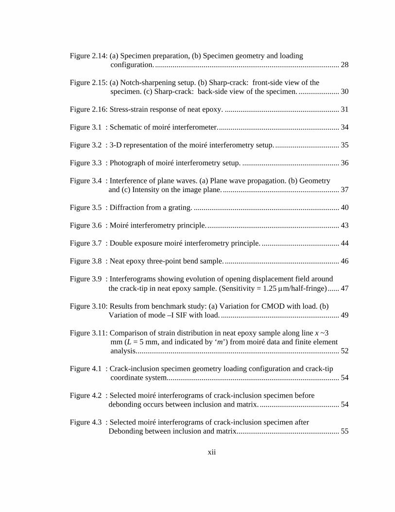
(4) Combination of some or all of previous three types.

In general a structure made of a composite material contains a binder material

known as the matrix phase and one or more reinforcing phases at the microscopic scale.

The secondary phase can be in the form of long fibers, whiskers or particles of different

geometries.

Long fibers (very high length-to-diameter ratio) generally being much stiffer and

stronger than the bulk material have found applications in fiber reinforced composite

materials. For example, strength of commercially available micron size glass fibers is

almost 140 to 240 times that of bulk glass. Common fiber reinforced plastics (FRP)

generally contain fibers such as carbon, boron or glass oriented in either unidirectional or

multidirectional architecture and bonded together by a polymer such as epoxy, polyester,

etc. They offer high strength-to-weight and strength-to stiffness ratios along with good

impact and fatigue resistance crucial to aerospace and military applications.

Accordingly, investigation of failure of fiber reinforced composites at various length

scales have received much attention in recent years.

Particle reinforced metal matrix composites (MMC) (such as, aluminum matrix

reinforced with silicon carbide (SiC) or titanium carbide (TiC) particles) have shown

great potential for many elevated temperature applications. As the name suggests

particulate composites involve discrete filler/reinforcement phase/s in a binder unlike

continuous fibers in FRPs. The use of particulates enables a cost effective production of

this class of composites while offering flexibility in terms of filler size, volume fraction,

shape and distribution to alter properties for a given application. Additionally, the

macroscopic isotropy of these composites greatly simplifies the mechanical design. The

3

Problem: Interaction of matrix crack

with embedded second phaseApplications

Ref: www.aviation-history.comFiber Reinforced CompositePolymer – Aircraft components

UnderfillDie Bumps

Solder Ball

Package A’A

Composite Micro-structure–Flip chip Package

Crack

FibersAA

Crack

Hollow Micro-spheres

Crack

Syntactic foam -BuoyRef: www.flotec.com

Figure 1.1: Some applications of composite materials and relevance of the crack-inclusion interaction study.

filler particles could also be either metallic (aluminum, silver, etc.) or non-metallic

(alumina, silica, etc.). For example, structural syntactic foam (Kirugulige et. al. [8]) is a

type of particulate composite in which prefabricated micro hollow spheres are dispersed

in a binder. In these foams porosity is microscopic unlike conventional foams and can be

varied by controlling the size and the density of hollow spheres in the matrix during

4

fabrication. Among the typical applications of syntactic foams are the high compression

applications such as undersea probes and marine platforms. The electronics industry also

utilizes particulate composites as underfill materials which are generally silica-filled

epoxy or urethane compounds are used to relieve stresses in electrical interconnects such

as solder ball grid array (BGA). One of the recent advances in particulate composites is

the development of the so-called Functionally Graded Materials (FGM) having

directional variations of their thermo-mechanical properties. This is achieved by varying

the volume fraction (and/or other micro-structural features) along a desired direction

during material processing. Techniques such as slip casting [2], centrifugal casting [3],

laser alloying and cladding [4], plasma-spray forming [5] and gravity casting [6, 7] have

been used successfully to fabricate such materials.

By combining of one or more types of composites discussed above gives numerous

variations of materials for structural applications. In view of these, it is important to

study failure of these materials in order to predict their thermo-mechanical performance

and reliability during service. Figure 1.1 shows some of the common applications

discussed in the previous section along with representative insets where potential crack-

inclusion interactions are possible. These generally include a matrix crack interacting

with a filler phase such as a reinforcing fiber or a particle.

1.2 The crack-inclusion interaction problem

The fundamental problem of a matrix crack interacting with a second phase

inclusion is of vital interest to researchers due to the increasing use of composite

materials and their complex failure behavior. Generally, the mechanical behavior of

5

composite materials depends mainly on properties of the individual phases involved and

the strength of the bond between them. As shown in Fig. 1.2 the intrinsic failure process

under the influence of a pre-existing or a service induced flaw (such as a crack) can be

explained by studying a simplified problem of a matrix crack interacting with the second

phase which can be a fiber or a particle. Simplifying the problem in this manner

facilitates parametric investigation of the problem for possible material design. Some of

these variations include (a) the geometry and the size of the inclusion, (b) the orientation

of the inclusion with respect to the crack, (c) the mismatch between elastic properties of

Figure 1.2: Schematic of a matrix crack interacting with an inclusion.

the matrix (Em, νm) and the inclusion (Ei, νi), (d) effects of bond strength between the

inclusion and the matrix and (e) a crack interacting with multiple inclusions.

Y

X

Z

X

Y

Matrix crack

Inclusion Ei, νi

Em, νm

6

1.3 Background and literature survey

Several investigations of the aforesaid problem have been carried out from both

analytical and numerical perspectives since the early study of its kind by Tamate [9].

Using Mushkelishvili’s complex potentials, he studied the interaction of a radial matrix

crack with a circular inclusion in a uniaxially loaded plate. He showed that a relatively

stiff inclusion ahead of a compliant matrix reduces the stress intensity factors whereas a

compliant inclusion ahead of a stiff matrix crack increases the same. Atkinson [10]

investigated the problem of a crack outside a perfectly bonded elastic inclusion under

uniaxial and biaxial tensions for different crack lengths and elastic properties of the

inclusion and the matrix. He solved singular integrals numerically to obtain the stress

intensity factor variations as a function of the distance between the inclusion and the

crack tip. Erdogan et. al. [11] investigated interaction between a circular inclusion and an

arbitrarily oriented crack using Green’s functions. They developed expressions for mode-

I and mode-II stress intensity factors in terms of asymptotic values of density functions of

integral equations which are given in terms of crack face displacements. Gdoutos [12, 13]

studied interaction between a crack and a hole or a perfectly bonded inclusion in an

elastic medium under uniform tension. He investigated critical values of the applied

stress for crack extension and initial crack extension angle in both the cases and reported

that rigid inclusion increases the fracture strength of the plate while the opposite occurs in

case of a hole. He also later studied stable crack growth when a crack is oriented along a

diameter of the inclusion using strain energy density theory. The investigation included

dependence of the stable crack growth on loading rate and showed that critical value of

failure stress decreases as the number of loading steps decreases (i.e. at higher loading

7

rates) and lower loading rates results in a more stable crack growth. Kunin and

Gommerstadt [14] used projection integral equation approach for studying a crack-

inclusion system and developed a relationship between J and M (where J is the energy

release rate and M is the interaction integral) integrals for translation of the inclusion with

respect to the crack and the effect of the inclusion size. Hasebe et. al. [15], studied stress

fields when debonding occurs between a rigid circular inclusion from the matrix and the

resultant interfacial crack in an infinite plate loaded in uniform tension. They modeled the

phenomena as a mixed boundary value problem and reported stress intensities at debond

tip. Patton and Santare [16] investigated interaction of a crack with elliptical inclusions.

They examined the problem using Mushkhelishvili’s complex potentials and used them

to formulate singular integral equations for crack opening displacement and solved for

stress intensity factors numerically. They studied the problem of a straight crack near a

rigid inclusion in an infinite medium. It was observed that for relatively flat elliptical

inclusions and radially oriented crack with respect to the inclusion, as the crack rotates

towards the flat side of the inclusion the crack tip stress intensity decreases drastically.

Li and Chudnovsky [17, 18] performed energy analysis and examined effects of an elastic

inclusion on the energy release rate for crack extension. They studied variations due to

inclusion translation, rotation and expansion with respect to the crack tip and showed that

a crack approaching a soft inclusion accelerated while a crack approaching a stiff

inclusion slowed down.

Boundary element (BE) methods have been used widely to address crack-

inclusion interaction problems. Bush [19] used BE formulation to model a matrix crack

interacting with single and multiple inclusions and reported crack paths and energy

8

release rates (ERR) for crack initiation and growth. This study showed that a crack tip

approaching a particle is shielded from far field stresses whereas after it passes the

inclusion the crack tip stresses are amplified. It was also observed that no substantial

crack deflection occurs until the tip is within approximately one radius away although

ERR effects are noticeable when the distance between the crack and the stiff inclusion is

about five radii. He also modeled a weak interface between an inclusion and matrix by

introducing a flaw between them and showed that the flaw increases ERR substantially

and attracts the crack. Knight et. al. [20] studied the effect of introducing an interphase

region between an inclusion and the matrix on ERR and crack trajectories using BE

technique. They studied effects of Poisson’s ratio of the inclusion and the matrix in the

absence of interphase and observed that as the Poisson’s ratio of the matrix approaches

incompressibility limit of 0.5, shielding effect and deflection experienced by the crack

reduces. They showed that the Poisson’s ratio of the inclusion being higher than that of

the matrix results in distinct shielding whereas amplification occurs in the opposite

scenario. Interphase thickness was shown to affect the crack behavior depending on the

relative elastic property mismatch between the three phases. Recently, Kitey et. al. [21]

and Kitey [22] investigated interaction between a crack and a single inclusion and a

cluster-of-inclusions using symmetric Galerkin BE method. They showed that a crack

propagating through a particle cluster exhibits different trajectories with respect to cluster

orientation whereas the overall energy dissipation remains unaltered. In this study it was

also observed that increase in the area ratio of inclusions to matrix increases ERR and

hence material becomes more fracture resistant.

9

Although many researchers have contributed analytically and numerically to the

problem, strikingly few experimental investigations are found in the literature owing to

the obvious experimental complexities. O’Toole and Santare [23] have investigated

crack-inclusion interaction experimentally using photoelasticity. They simulated an

inclusion by bonding rather than embedding two identical steel inclusions on two

opposite faces of a polycarbonate plate ahead of a crack. Influence of elliptical

inclusions on an edge crack was studied by calculating stress intensity factors from

experimental data and showed toughening effect to be the greatest for an elliptical

inclusion when its major axis is normal to the crack plane. Another interesting

experimental study of the problem is by Li et. al. [24]. They experimentally modeled

perfectly bonded ‘second phase’ in a matrix by altering the chemical structure by

selectively exposing specific regions of a polymer to UV radiation. Under fatigue

loading conditions, they experimentally measured crack speed and qualitatively observed

fractured surface morphology. They reported energy release rates and crack speeds for a

crack approaching and penetrating softer inclusion and showed that interaction with a soft

or a stiff inclusion affects the resulting crack path significantly. Single fiber pull-out test

is used to characterize interfacial properties of fiber-matrix bond, namely interfacial

fracture energy (in shear dominated failure) and shear stress. Easley et. al. [25] used

moiré interferometry to investigate stress field in a fiber pull-out test in the presence of

nearby matrix cracks when the crack plane is perpendicular to the axis of the fiber.

Specimens with partially exposed fibers were used to investigate shear stress in the

vicinity of the fiber and the crack. They reported a decrease in shear stress near the fiber-

matrix interface at peak pullout load.

10

A perfect bond between a matrix and an inclusion seldom exists in reality due to

finite interfacial strength. This results in interfacial debonding between the two which in

turn plays a significant role in the overall failure process. The presence of a nearby crack

would likely aggravate or accelerate the process as well. Apart from the interfacial bond

strength, debonding may depend on material properties of the matrix and the inclusion,

geometry of the crack-inclusion pair and the type of loading. The matrix-inclusion

debonding causes redistribution of strains and hence stresses in the vicinity of both the

inclusion and the crack. These make it important to study and model mechanical fields in

the vicinity of a crack-inclusion pair as debonding evolves. Debonding of the inclusion

matrix can be easily detected if full-field displacements are measured. None of the

reported investigations address this very important issue of matrix-inclusion debonding in

presence of a nearby crack. Dearth of experimental investigations regarding this issue

emphasizes the need for further investigation in this regard. Also, experimental

investigation of this problem can offer valuable insight for developing numerical models

and help achieve reliable solutions.

1.4 Objectives

As discussed in the previous Section, the issue of debonding of a matrix from an

inclusion in the presence of a crack requires further experimental investigation. Optical

techniques are extensively used for mapping full-field deformations in various solid

mechanics problems. Among these techniques moiré interferometry is a well-known

whole field experimental tool used to study in-plane displacement and strain fields. This

technique in its various forms has been employed to study macro and micro mechanics

11

problems by many researchers. To be able to employ this technique successfully,

fabrication of physical specimen gratings of desired spatial frequency in the region of

interest is of key importance. Microlithography processes are extensively adopted in

recent years by microelectronics and MEMS industries to fabricate micro and nano

features on different substrates. The most common substrate used is silicon which is

commercially available in the form of wafers. Microfabrication of gratings on a silicon

wafer is a well-known process that uses photolithography and can be used to fabricate

gratings on specimen substrates. Considering all the requirements of the stated problem

and the availability of resources, the main objectives identified for this research are as

follows:

• Fabricate square-wave profile gratings on silicon wafer and devise reliable

method/methods to transfer gratings to specimens.

• Fabricate a specimen to study the crack-inclusion interaction problem in a two-

dimensional setting.

• Develop a moiré interferometer to map full-field displacement fields in real-time

and extract strains at strategic locations in the vicinity of a crack-inclusion pair.

• Measure fracture parameters such as crack opening displacements and stress

intensity factors (K), energy release rates (ERR) under quasi-static loading

conditions and identify matrix-inclusion debonding.

• Model matrix-inclusion debonding in the crack tip vicinity using finite element

method and experimentally validate the model.

12

• Parametrically study crack-inclusion interaction using the validated finite element

model.

1.5 Organization of the thesis

Including the current chapter this thesis comprises of five chapters. Chapter 2

presents details of the microfabrication used to develop silicon wafer gratings. In this

chapter the methods developed to fabricate the specimen gratings are elaborated. This

chapter also describes fabrication of crack-inclusion specimen for experimental study.

Chapter 3 discusses the basics of interference of light waves and the working principle of

moiré interferometry. Results of benchmark experiment with homogeneous cracked

sample (without inclusion) are presented in this chapter. The experimental investigation

of the crack-inclusion interaction problem using moiré interferometry is described in

Chapter 4. Chapter 5 describes a finite element methodology to simulate crack-inclusion

interaction including the method used to model debonding between an inclusion and a

matrix. This chapter also covers comparison between experimental and numerical results

followed by a parametric study for the crack-inclusion problem using the adopted

methodology. Chapter 6 concludes the work with a summary of observations and

outcome of the thesis work.

13

CHAPTER 2

GRATINGS FABRICATION AND TRANSFER TECHNIQUES

A critical requirement for successfully implementing moiré interferometry is to

have high quality gratings printed on the specimen. Modern day lithography processes

have been used in the current work to fabricate amplitude gratings on silicon wafers.

Two methods are developed to transfer gratings to specimens. Photolithography is the

underlying methodology used here to achieve the desired patterns [26]. It involves

transfer of geometric shapes on a mask to a substrate coated with photosensitive polymer

called photoresist. Accounts of various other methods used to develop and print gratings

on specimens for moiré interferometry can be found in works by Post [27] and his co-

researchers. Among these, a method extensively used now-a-days involves fabrication of

a master (sinusoidal) grating using high spatial frequency interference pattern of

photoresist. The photoresist is developed following exposure to create a master grating.

Replicas made from master gratings are used to create specimen gratings after depositing

a reflective aluminum layer on them. In the current work photolithography technique is

used in conjunction with various microelectronic fabrication tools and methods to create

‘square-wave’ amplitude gratings on a silicon wafer. This process is executed in various

steps and requires a careful control over the process parameters to achieve the

desired results. Next the various necessary steps are described.

14

(a)

(b) (c)

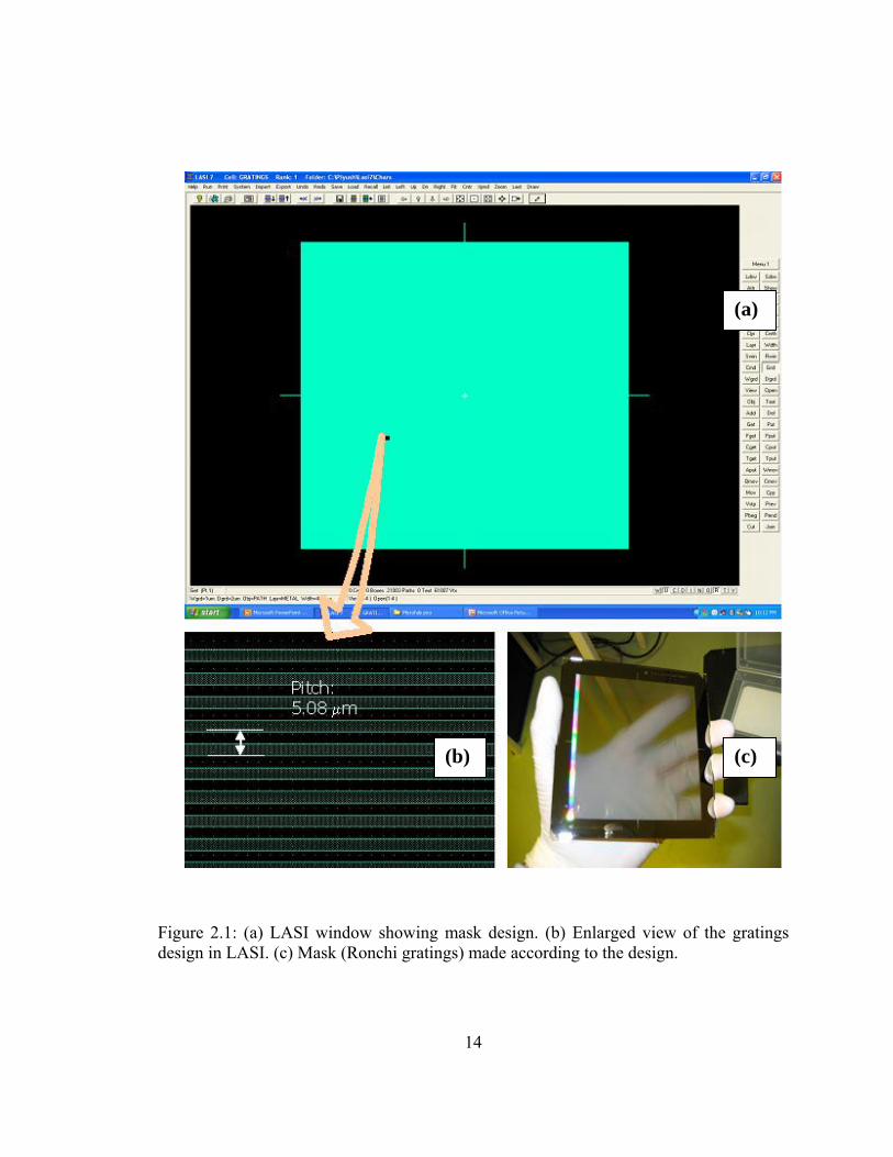
Figure 2.1: (a) LASI window showing mask design. (b) Enlarged view of the gratings design in LASI. (c) Mask (Ronchi gratings) made according to the design.

15

2.1 Master gratings fabrication

Considering the availability of in-house microfabrication facilities, a spatial

frequency of 5000 lines/inch (5.08 µm pitch) was adopted. A mask was first designed

using LASI (LAyout System for Individuals), a general purpose IC layout freeware and

design system. A chrome-on-glass mask (essentially a Ronchi grating) with equally

spaced opaque chrome bars and transparent glass spaces was procured from a commercial

source based on the supplied design. Figure 2.1(a) shows the LASI design window used

for the mask design. In Fig. 2.1(b) an enlarged view of the grating pattern to be produced

on the mask is shown. Figure 2.1(c) shows the actual mask thus procured. The active

area of the mask has dimensions of 4 inch x 4 inch and it can be used to process a 4 inch

diameter silicon wafer utilizing the full wafer area.

A single side polished, P-type <100> silicon wafer (diameter = 100 mm, thickness

= 1 mm) was used for producing master gratings. (The crystallographic orientation and

Figure 2.2: (a) Wafer cleaning. (b) Dehydration bake.

16

doping are not critical for the present work and were simply based on the availability.)

The polished surface of the wafer was used for all processes described in the following.

The wafer surface was rinsed with Acetone (Dimethyl Ketone CH3-CO-CH3) generously

followed by a quick rinse with Methanol (Methyl alcohol CH3-OH) and then dried using

pressurized nitrogen (see Fig. 2.2(a)). Next the wafer was baked at 120 oC for 20 min, to

remove any moisture (Fig. 2.2(b)). Then HMDS (Hexamethyl-Disilazane) - a primer that

enhances adhesion between silicon and photoresist - was vaporized onto the wafer

surface in a closed container for about 20 minutes (Fig. 2.3(a)). After centering the wafer

on a vacuum chuck a positive photosensitive polymer (photoresist-AZ5214) was spin

coated on the prepared wafer surface at 3500 RPM for 30 seconds as shown in Fig 2.3(b).

This results in a (~ 1.5 µm thick) layer of photoresist over the wafer surface. To let the

photoresist cure quickly the wafer was then soft baked on a hot plate at 105 oC for 60

seconds with the rough side of the wafer in contact with the hot plate surface (Fig.

2.4(a)).

Next the photoresist was exposed using the mask in a mask aligner (Karl Suss

Model # MA6) with an exposure time of 6-8 seconds. UV radiation is used in the mask

aligner (Fig. 2.4(b)) for exposing the photoresist. A hard contact was used between the

mask and the wafer during exposure.

The exposed wafer was then developed (Fig. 2.5(a)) in a 1:2 solution of developer

AZ 400K and water for approximately 20 seconds. Then the wafer was quickly rinsed

deionized water (Fig. 2.5(b)) for 2 minutes, dried using pressurized nitrogen (Fig. 2.5(c))

and inspected under an optical microscope (Fig. 2.5(d)). The development of the

photoresist results in a regularly spaced photoresist bars with bare silicon spaces in

17

Figure 2.3: (a) HMDS application. (b) Photoresist application.

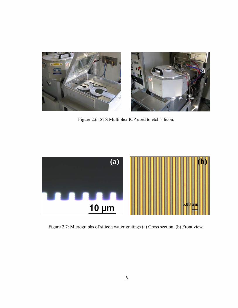
Figure 2.4: (a) Soft baking of the wafer. (b) The mask aligner showing the mask and the wafer. (Mask is held in the frame by vacuum.) between them. The developed wafer was then anisotropically etched in those bare silicon

spaces using Inductively Coupled Plasma (ICP) (STS Multiplex ICP). An in-built

program ‘MORGANSOI’ was used for this purpose for 4 cycles of alternative passivation

and etching. Each consecutive etching cycle affects the passivation layer on horizontal

surfaces but the vertical walls are almost unaffected during etching. This results in a very

18

high quality anisotropic etching with almost square wave profile gratings on silicon

wafer. Approximately 2 µm etching depth was achieved. The photoresist bars were then

stripped off from the wafer using oxygen plasma using a photo-stripping machine

(MATRIX). An in-built program ‘Photo-Str’ was used and the process time used was

approximately 4 minutes. At the end of this step a high quality square-wave grating

Figure 2.5: (a) Photoresist development (b) Rinsing (c) Drying (d) Inspection under microscope.

was generated on the wafer surface with the desired pitch of 5.08 µm. Then using the

same ICP machine a very thin passivation layer (C4F8) was deposited on the gratings

using a program ‘PASSIVAT’ for 6 minutes. The silicon wafer gratings were then

examined under a microscope and critical dimensions were measured using an in-built

19

Figure 2.6: STS Multiplex ICP used to etch silicon.

Figure 2.7: Micrographs of silicon wafer gratings (a) Cross section. (b) Front view.

5.08 µm

(b) (a)

20

Figure 2.8: Schematic of steps involved in fabrication of silicon wafer gratings.

(f) Stripped photoresist

(g) Application of passivation layer

(e) Etching of silicon

(a) Silicon wafer

(b) Application of photoresist

(d) Development of photoresist

(c) UV exposure using grating mask

Mask

21

digital camera. The micrographs of silicon wafer gratings are shown in Fig. 2.7. Figure

2.8 shows a schematic of all the processes discussed so far.

2.2 Grating transfer methods

To prepare specimen gratings from master gratings two different techniques were

developed in this work. Both the techniques were tested successfully and are described

in detail next.

2.2.1 Direct grating transfer from a silicon master

In this method a thin aluminum layer was vacuum deposited on the silicon wafer

after the gratings were prepared as described earlier. This was done using a Denton

Vacuum Deposition machine under high vacuum of (2 X 10-5 torr). A photograph of a

silicon wafer grating with aluminum film deposited over it is shown in Fig. 2.9. The rest

of the steps involved in grating transfer are depicted schematically in Fig. 2.10.

Figure 2.9: Aluminum coated silicon wafer gratings.

22

Figure 2.10: Direct transfer of gratings from silicon wafer with aluminum coating. (Note: In the schematic the specimen and the wafer are shown in thickness dimensions.)

(a) Specimen

Aluminum coating

Epoxy pool

Silicon wafer

(b)

(c)

Cured epoxy gratings with Al-coating

(d)

23

The fluorocarbon passivation layer (C4F8) (see, section 2.1) acts as a parting layer

between aluminum and silicon by reducing the adhesion strength between the two. The

specimen surfaces on which gratings were being transferred were prepared using #220

and then #320 grit sand papers. A pool of liquid epoxy was applied to the specimen

surface in the region of interest as shown in Fig. 2.10(a). The silicon master with the

desired orientation of the gratings with respect to the specimen was pressed against the

epoxy pool. Excess epoxy was removed and the pair was allowed to cure at room

temperature for about 72 hours. After the epoxy was cured silicon wafer was carefully

pried off without much effort. This resulted in gratings along with aluminum coating

transferred to the specimen surface with a high degree of fidelity (Fig. 2.10(c)) and good

reflectivity. (The use of thick (1 mm) wafer was helpful in handling of the wafer when

being pried off the specimen surface.) The silicon wafer was re-used to print gratings on

other specimens after redepositing the passivation layer and aluminum over it. A

specimen prepared in this manner is shown in Fig. 2.10(d) with high quality grating

structure in the region of interest.

2.2.2 Grating transfer using silicone rubber submasters

In the second method, silicone rubber was used to make submasters or replicas of

the master grating pattern on silicon wafer. A cardboard mold with its sides parallel and

perpendicular to the grating lines was prepared to create a stamp to replicate the gratings

from silicon wafer to the specimen. A photograph of the mold on silicon wafer and

prepared silicone rubber stamp (or submaster) with gratings on them is shown in Fig.

2.11. The steps involved in transferring gratings from the silicon wafer to a specimen is

24

shown schematically in Fig. 2.12. After preparing a card-board mold, 2 part silicone

rubber∗ was mixed thoroughly and liquid rubber was deaerated in a vacuum chamber at ~

25 inches of mercury until the rubber pool rises initially and trapped air bubbles collapse

eventually. Deaeration was continued for an additional 3-4 minutes. The liquid rubber

was then transferred into the mold and cured at room temperature for over 16 hours (Fig.

2.12(a)). The cured rubber submaster was then detached from the silicon wafer with

ease. A glob of liquid epoxy† was then deposited on a pre-fabricated epoxy specimen

surface (prepared with #220 and #320 grit sand papers) in the region of interest (Fig.

Figure 2.11: Silicone rubber casting molds and submasters.

∗Two-part silicone rubber (Plastisil 73-60 RTV) manufactured by Polytek Inc., PA. †Two-part epoxy (Epo-ThinTM (Product # 20-1840, 1842, )) 100 parts resin : 39 parts hardener) from Beuhler Inc., PA.

Molds Silicone rubber submasters

25

Figure 2.12: Steps involved in fabrication of silicone rubber submaster grating and transferring grating pattern onto specimen surface. (Note: specimen and grating are shown in the thickness dimension)

Silicon wafer

Liquid silicone rubber

Mold

(a)

Cured silicone rubber

Epoxy pool

Specimen

(b)

(c)

Cured epoxy gratings

(d)

(e)

26

2.12(b)). The silicone rubber submaster, with its edges aligned with the machined

specimen edges, was pressed against the specimen surface and excess epoxy was

squeezed out (Fig 2.12(c)) and removed using cotton swabs. Finally after epoxy was

cured the rubber mold was detached from the specimen with little effort (Fig 2.12(d)).

This resulted in high quality amplitude gratings on the specimen surface.

Figure 2.13: Micrographs of (a) Cross-section of a silicone rubber submaster (b) Front view of epoxy gratings transferred using a silicone rubber submaster.

Relatively high diffraction efficiency was obtained from these gratings as evident

from high quality moiré interferograms to be discussed. (Depositing a reflective metallic

film (aluminum, gold, etc.) is optional for studying dynamic events where high

reflectivity is needed.) This method allowed fabrication of virtually unlimited numbers

of submasters and was also tested successfully on both metallic and polymeric substrates.

A specimen with epoxy gratings transferred using this method is shown in Fig. 2.12(e).

The cross-section of a silicone rubber stamp as viewed under an optical microscope is

shown in Fig. 2.13(b).

27

2.3 Crack-inclusion specimen fabrication

Next, specimen preparation for crack-inclusion interaction studies is described. To

simulate this problem in a two dimensional setting, epoxy was used as the matrix material

and laboratory grade glass was used as the inclusion. The elastic properties of the matrix

and the inclusion phases are listed in Table – 2.1. Pyrex glass rods of diameter 3.8 mm

Table 2.1: Elastic properties of matrix and inclusion.

were cut into cylindrical pieces of length 7.1 mm. To enhance bond strength between

glass and epoxy, glass cylinders were treated with gamma-aminopropyltrimethoxysilane‡

according to manufacturer’s instructions. This bonding agent is used widely in the

fabrication of glass-filled polymeric composites to improve matrix-filler bonding

strength. The glass cylinder was then held in a mold of cavity thickness equal to its

length so that the axis of the cylinder was perpendicular to the major dimensions of the

mold (see, Fig. 2.14(a)). Two part epoxy mixture was then poured into the mold around

the inclusion and cured at room temperature for about 72 hours. The cured sample was

then machined to the required dimensions and epoxy gratings were printed using one of

the methods described previously. (It should be noted that, gratings and specimen

materials being same, shear lag effects are minimum.) Figure 2.14(b) depicts specimen

geometry, dimensions and loading configuration with an illustration of grating lines and

orientation on them. Here L is the distance between the crack tip and the center of the ‡ Silquest A-1110 Silane manufactured by GE Silicones, WV.

Young’s modulus E (GPa)

Poisson’s ratio ν

Epoxy 3.5 0.35 Glass 68 0.19

28

inclusion of diameter d. Thus L/d ratio is a nondimensional measure of inclusion

proximity to the crack tip and it was 1.31 in this work. A notch was then cut into the

edge of the specimen using a circular diamond impregnated saw blade (thickness

Figure 2.14: (a) Specimen preparation, (b) Specimen geometry and loading configuration.

Specimen

a = 8.5 mm W = 42.5 mm B = 7.1 mm d = 3.8 mm L = 5 mm S = 127 mm

W

B

La

d

S

P

Epoxy beam

Glass inclusion

Gratings

Crack

(b)

(a)

Epoxy

Glass inclusion

Mold

29

~300 µm). To sharpen the notch-tip a set-up was developed and is shown in Fig. 2.15(a).

The set-up includes a translation stage with micrometers mounted on an angle bracket

with a sharp razor blade fixed vertically, as shown. The specimen was rested on a fixed

stage with horizontal and vertical support surfaces. The thickness of the blade being less

than the notch width, it was driven freely into the notch. The sharp edge of the blade was

then pressed into the notch tip in a controlled manner for approximately 200 µm depth.

The blade was then retracted while holding the specimen against the supports resulting in

a sharpened notch tip shown in the micrographs in Figs. 2.15(b) and (c). By careful

alignment of the blade with respect to the translation stage the length difference of the

sharp crack on the front and back sides at the notch tip was controlled to within ±30 µm.

2.4 Materials characteristics

Epoxy used in this work as the matrix material was initially characterized by

performing a uniaxial tension test on a ‘dog-bone’ specimen. The test was performed in a

INSTRON 4465 testing machine and the results are shown in Fig. 2.16. The strain was

measured using an extensometer (Epsilon Inc., model # 3542-0050-010-ST). The initial

response shows that epoxy used here is essentially a linear elastic material with a modest

nonlinearity seen before failure. The elastic modulus determined from the graph by

drawing a tangent to the initial part of the curve is 3.4 ± 0.1 GPa. Evidently, the strength

of epoxy is approximately 63 ± 2 MPa and failure strain is 0.02 ± 0.002.

30

(a)

(b) (c)

Specimen

Translation stage

Razor blade

Figure 2.15: (a) Notch-sharpening setup. (b) Sharp-crack: front-side view of the specimen. (c) Sharp-crack: back-side view of the specimen.

31

Figure 2.16: Stress-strain response of neat epoxy.

ε0.000 0.005 0.010 0.015 0.020 0.025

σ ( M

Pa)

0

10

20

30

40

50

60

Neat epoxy

32

CHAPTER 3

MOIRÉ INTERFEROMETRY

Moiré fringes are interference patterns generated when two geometric patterns of

nearly same spatial frequency are superimposed. Though considered optical noise in

many instances moiré patterns are used in the field of solid mechanics to measure in-

plane and out-of-plane deformations. An interferometric version of this method called

moiré interferometry is used in the current research to map in-plane displacement

components in real-time. This method has been used successfully to study macro- and

micro-mechanics problems in engineering. These encompass fracture mechanics,

mechanics of microelectronic packages, composite materials, bi-material joints and for

calibrating strain measuring devices, to name a few.

In the current work moiré interferometry is utilized to map evolution of dominant

displacement fields in the vicinity of a crack-inclusion pair. Moiré interferometry

depends on both interference and diffraction of coherent light. Two coherent light beams

with plane wave fronts interfere to produce periodic constructive and destructive intensity

patterns or the so-called virtual gratings. The working principle, implementation issues

and various applications of moiré interferometry are detailed in a monograph by Post [27,

28]. This chapter explains the optical setup developed for the current investigation, the

33

associated mathematical analysis of moiré interferometry [29, 30], validation experiments

and results.

3.1 Experimental Setup

Figure 3.1 shows a schematic of the optical setup developed during this research.

It includes a 8 mW He-Ne laser, Ronchi grating (R), mirrors (M1, M2, M3 and M4),

collimators (C1 and C2), lens (L1) and a CCD camera. The Ronchi grating R is of the

same pitch as the specimen gratings to easily achieve the required angles of incidence on

the specimen. The unexpanded laser beam was made to pass through the Ronchi gratings

(with its principal axis in the horizontal plane, in this case) using mirror M1. Upon

transmission laser beam undergoes diffraction and several odd diffraction orders in the

horizontal plane are generated. The angle α between diffraction orders is given by the

diffraction equation,

sinpλα , (3.1)

where λ is the wave length of light and p is the pitch of the Ronchi gratings. For He-Ne

laser (λ = 633 nm) and a grating pitch of 5.08 µm, the value of α is ~7.15o. All but ±1

diffraction orders were blocked by an aperture and the first order diffractions were

directed towards mirrors M2 and M3. The reflected laser beams were then directed into

two separate beam expanders coupled to collimators C1 and C2 as shown. The

collimators were mounted on x-y-z translation stages for fine adjustment. The expanded

and collimated laser beams (with plane wave fronts) were directed towards the specimen

as shown and made to interfere with each other producing a standing wave of pitch

34

Figure 3.1: Schematic of moiré interferometer.

Power supply

Loading Control unit

Data logger

Loading tup Computer

Specimen

Plane wave front

Distorted object wave front

R

45o M1 He-Ne Laserλ = 633 nm

CCD Camera

M4

L1

M3 M2

α

α C2 C1

+3 -3 +1 -1

0

35

pv = 2.54 µm (10000 cycles/inch) on the specimen surface. These two incident beams are

diffracted by the specimen grating and produce ±1 diffractions propagating along the

optical axis (dotted line ) towards mirror M4 and the camera carrying information

about in-plane deformations shown by warped wave fronts in Fig. 3.1. They are directed

into the camera back by the mirror M4 and imaging lens L1. The recording system

consisting of the lens and the camera back is kept focused on the specimen plane. For

further clarity a three dimensional sketch of the setup is shown in Fig 3.2 and an actual

photograph of the setup is shown in Fig. 3.3.

Figure 3.2: 3-D representation of the moiré interferometry setup.

A null field was achieved in no-load condition by making fine adjustments to the

collimators. The +1 and -1 orders emerging from the specimen grating and propagating

along the optical axis interfere and produce moiré fringes. The details of the optical

7.1

0o Mirror

0o Mirror

Collimator

Collimator

He-Ne Laser

45o MirrorGrating (Pitch= 5.08 µm)

0

-3

+3

-1

+1 y, v(x, y)

Specimen

Data Acquisition

x, u(x, y) Digital Camera

Time

Load

Computer

Focusing Lens

45o Mirror

36

analysis are presented in the next section. These fringes represent contours of in-plane

displacement component in the principal direction of the specimen grating. In the current

Figure 3.3: Photograph of moiré interferometry setup.

investigation crack opening displacements (displacements in the y-direction) were

mapped. The opening displacements are governed by the equation,

( , ) ( , ) ,y vv x y N x y p= Ny = 0, ±1, ±2, ±3,… (3.2)

where Ny represents fringe orders and pv (= 2.54 µm) is the pitch of the virtual gratings

Data logger

Mirror

Collimators

Loading frame

SpecimenLens

Camera

Mirror

Ronchi rulings

Mirror

He-Ne laser

37

3.2 Deformation field mapping

The specimen was placed in a loading frame and a null light field was achieved

under no-load conditions. A digital CCD camera interfaced with a computer was set to

time-lapse photography mode to record interferograms at 2 seconds intervals during the

loading phase. A load cell connected to a data logger was also interfaced with the same

computer and was configured to log the load history at a rate of 5samples/sec during the

event. Both the camera and the data logger were triggered from the computer at the same

time as the loading phase was initiated. The specimen was loaded quasi-statically in

three-point bending configuration in a displacement control mode with a cross-head

speed of ~0.04 mm/sec. The recording camera was configured in a manner that each

image was tagged with temporal information of the computer clock as images were

dumped into the computer memory. The data logger clock was also synchronized with

the computer clock such that loading data and the corresponding time for each data point

was recorded. This facilitated establishing load levels at which each image was recorded.

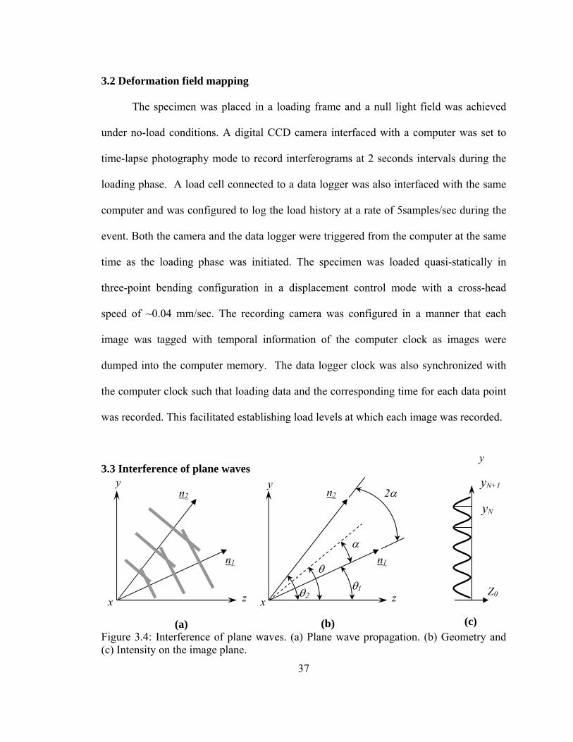
3.3 Interference of plane waves

Figure 3.4: Interference of plane waves. (a) Plane wave propagation. (b) Geometry and (c) Intensity on the image plane.

(a)

y

z

n1

n2

x

(b)

n2

n1

y

z

θ θ1 θ2

α

x

2α

(c)

yN

yN+1

Z0

y

38

Let us consider two plane waves with propagation vector represented by n1 and

n2 shown in Fig 3.4 and their respective angles with the z –axis as θ1 and θ2. Τhese

plane waves can be represented in vectorial forms as,

1

2

.1 1

.2 2

ikn s

ikn s

Ae

A e

ψ

ψ

=

= (3.3)

where ψ1 and ψ2 denote complex amplitude distributions and s is the position vector.

Considering propagation in the y-z plane, y zs ye ze= + where ye and ze are unit

vectors in y and z- directions, respectively and 2k π λ= is the wave number. Here, A1

and A2 represent strength of the field and λ is the wave length. Using the angular

parameters shown in Fig. 3.4(b), complex amplitudes can be expressed as,

1

2

1 1 1 1 1

2 2 2 2 2

exp[ ( sin cos )]

exp[ ( sin cos )]

i

i

A ik y z Ae

A ik y z A e

φ

φ

ψ θ θ

ψ θ θ

= + =

= + = (3.4)

where 1 1 1( sin cos )y zφ θ θ= + and 2 2 2( sin cos )y zφ θ θ= + . If the field strengths of the

above two wave fronts are same, then A1 = A2 = A. Then,

1 2totalψ ψ ψ= + 1 2( )i iA e eφ φ= + and the resulting intensity is given by the scalar product,

*total totalI ψ ψ= ⋅

where *totalψ denotes complex conjugate of totalψ . Hence,

1 2 1 22 ( )( )i i i iI A e e e eφ φ φ φ− −= + +

22 (1 cos )A φ= + ∆ s (3.5)

where,

39

1 2φ φ φ∆ = − 1 2 1 2[ (sin sin ) (cos cos )]k y θ θ θ θ= − + − (3.6)

is the phase difference.

From Fig. 3.4(b), 1θ θ α= − , 1θ θ α= + . Substituting these in eq. (3.6),

( ) ( ){ } ( ) ( ){ }sin sin cos cosk y zφ θ α θ α θ α θ α⎡ ⎤∆ = − − + + − − +⎣ ⎦

2 sin ( cos sin )k y zα θ θ= − + (3.7)

By installing the origin on the specimen surface (z = 0 on the specimen), we get,

0 2 sin cosz kyφ α θ=∆ = − . (3.8)

By combining eq. (3.7) with eq. (3.4), it can be said that intensity attains maximum value

(= 4A2) when 2Nφ π∆ = , where N=0, ±1, ±2...

Hence, 2sin cosN

Ny λα θ

= and 1

( 1)2sin cosN

Ny λα θ++

= are locations of two consecutive bright

fringes and the associated fringe spacing is,

1 2sin cosN N vy y p λα θ+− = = , (3.9)

where pv is fringe spacing or the pitch of virtual gratings in case of two beam moiré

interferometry in this study. For 0θ = ,

2sinvp λα

= . (3.10)

Thus in moiré interferometry setup of the current work the virtual grating

(reference) pitch is half of the initial pitch of the specimen gratings.

40

3.4 In-plane moiré interferometry

Single beam incidence

Figure 3.5: Diffraction from a grating.

The aperture function of a square wave (amplitude) gratings can be represented as,

2 2 2( , ) cos cos3 cos5 ...y y yt x y A B C Dp p pπ π π⎛ ⎞ ⎛ ⎞ ⎛ ⎞

= + − + −⎜ ⎟ ⎜ ⎟ ⎜ ⎟⎝ ⎠ ⎝ ⎠ ⎝ ⎠

As it is evident from the following analysis, truncating the series after the two terms is

sufficient to develop the necessary expressions for moiré interferometry. That is,

2( , ) cos yt x y A Bpπ⎛ ⎞

+ ⎜ ⎟⎝ ⎠

( )2 2

2i y p i y pBA e eπ π−= + + (3.11)

y

θ

θ

α α

Ψr, 0

Ψr, -1

Ψr, +1

Ψi

Ψr, +3

Ψr, -3 α

p

Object/ Specimen

41

Undeformed specimen

As shown in Fig. 3.5, if the gratings are illuminated by a plane wave represented by,

( sin cos )ik y zi Re θ θψ += where R is constant.

sin0

ikyi z Re θψ = = (3.12)

After reflection,

0i r ztψ ψ ==

( )sin 2 2iky i y p i y pRe A Be Beθ π π−= + + .

Expressing wave number as 2k πλ

= ,

sin 1 sin 12 22 sin /

0

i y i yp pi y

r z ARe BRe BReθ θπ π

λ λπ θ λψ⎛ ⎞ ⎛ ⎞

+ −⎜ ⎟ ⎜ ⎟⎝ ⎠ ⎝ ⎠

= = + + (3.13)

( ,0) ( , 1) ( , 1)r r rψ ψ ψ+ −= + +

where the second subscript in each term denotes the diffraction order of the wave. But, it

is known that for a grating with pitch p and wave length λ, diffraction angle α can be

represented as, sinpλα = . Therefore,

2 sin 2 (sin sin ) 2 (sin sin )0

i y i y i yr z ARe BRe BReπ θ λ π θ α λ π θ α λψ + −

= ⎡ ⎤= + +⎣ ⎦ (3.14)

Each term in eq. (3.14) represents diffracted waves propagating in distinctly different

directions given by multiples of the diffraction angle α. If the illumination angle θ, is

adjusted such thatθ α= ,

2 sin 2 (2sin )0

i y i yr z ARe BRe BRπ θ λ π α λψ = ⎡ ⎤= + +⎣ ⎦ (3.15)

42

where 2 sin( ,0)

i yr ARe π θ λψ = , 2 (2sin )

( , 1)i y

r BRe π α λψ + = and ( , 1)r BRψ − = . That is, ( , 1)rψ − is a

wave propagating in the z-direction towards the imaging device.

Deformed specimen

The specimen grating pitch p changes when the object deforms. Using prime

notation for quantities after deformation, deformed pitch p’ = p ± ∆p, where change in the

pitch is ∆p ≡ ∆p(x, y).

Then, 1 sin ''p

αλ

= where ' '( , )x yα α= .

The counterpart of eq. (3.15) upon deformation is,

sin (sin sin ') (sin sin ')0' ik iky iky

r z ARe BRe BReθ θ α θ αψ + += ⎡ ⎤= + +⎣ ⎦ (3.16)

where sin( ,0)' ikr ARe θψ = , (sin sin ')

( , 1)' ikyr BRe θ αψ +

+ = and (sin sin ')( , 1)' ikyr BRe θ αψ +

− = are the

amplitudes of the diffracted wave fronts.

Dual beam incidence

As shown in Fig. 3.6, when the deformed object is illuminated by two coherent

plane waves (or, collimated light beams) at angles +θ and -θ (that is α = θ), then,

sin1 0

sin2 0

ikyi z

ikyi z

Re

Re

α

α

ψ

ψ=

−=

=

= (3.17)

The diffracted wave fronts from the first beam are,

43

' sin (sin sin ') (sin sin ')1

ik iky ikyr ARe BRe BReθ θ α θ αψ + +⎡ ⎤= + +⎣ ⎦

( 1,0) ( 1, 1) ( 1, 1)' ' 'r r rψ ψ ψ+ −= + +

Similarly the diffracted wave fronts due to the second incident beam are,

Figure 3.6: Moiré interferometry principle.

' sin (sin sin ') (sin sin ')2

ik iky ikyr ARe BRe BReθ θ α θ αψ − − + − +⎡ ⎤= + +⎣ ⎦

( 2,0) ( 2, 1) ( 2, 1)' ' 'r r rψ ψ ψ+ −= + +

In Fig. 3.6 only ( 1, 1)' rψ − and ( 2, 1)' rψ − orders are shown for clarity. These two waves

propagate along the optical axis (z-axis), towards the imaging device (a camera). The

total complex amplitude registered on the camera plane is given by,

( 1, 1) ( 2, 1)' 'camera r rψ ψ ψ− −= +

(sin sin ') (sin sin ')( )iky ikyBR e eθ α θ α+ − += +

The corresponding intensity distribution on the image plane is given by,

*camera camera cameraI ψ ψ= ⋅

α

α

Ψi2

Ψi1

Ψ’r1,-1

Ψ’r2,-1 z

y

p

44

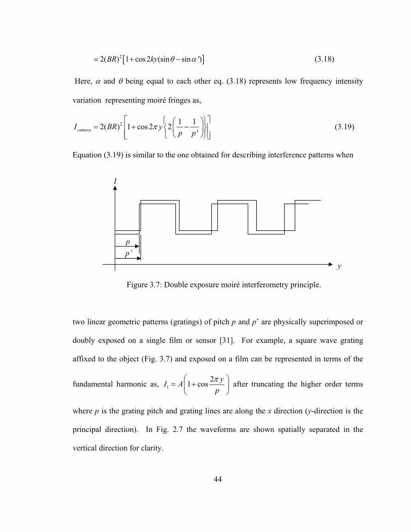
[ ]22( ) 1 cos 2 (sin sin ')BR ky θ α= + − (3.18)

Here, α and θ being equal to each other eq. (3.18) represents low frequency intensity

variation representing moiré fringes as,

2 1 12( ) 1 cos 2 2'cameraI BR y

p pπ

⎡ ⎤⎧ ⎫⎛ ⎞= + −⎢ ⎥⎨ ⎬⎜ ⎟

⎢ ⎥⎝ ⎠⎩ ⎭⎣ ⎦ (3.19)

Equation (3.19) is similar to the one obtained for describing interference patterns when

Figure 3.7: Double exposure moiré interferometry principle.

two linear geometric patterns (gratings) of pitch p and p’ are physically superimposed or

doubly exposed on a single film or sensor [31]. For example, a square wave grating

affixed to the object (Fig. 3.7) and exposed on a film can be represented in terms of the

fundamental harmonic as, 121 cos yI A

pπ⎛ ⎞

= +⎜ ⎟⎝ ⎠

after truncating the higher order terms

where p is the grating pitch and grating lines are along the x direction (y-direction is the

principal direction). In Fig. 2.7 the waveforms are shown spatially separated in the

vertical direction for clarity.

I

yp’ p

45

If the grating upon loading changes its pitch locally to p’ the changed profile can

be expressed as 2 ,

21 cos yI Apπ⎛ ⎞

= +⎜ ⎟⎝ ⎠

. If a single film records both unchanged and

changed profile the resulting intensity is expressed as,

1 2 ,

2 22 cos costotaly yI I I A

p pπ π⎛ ⎞

= + = + +⎜ ⎟⎝ ⎠

, ,

1 1 1 12 1 cos 2 cos 2A y yp p p p

π π⎛ ⎞⎛ ⎞ ⎛ ⎞

= + + −⎜ ⎟⎜ ⎟ ⎜ ⎟⎝ ⎠ ⎝ ⎠⎝ ⎠

(3.20)

In eq. (3.20) ,

1 1cos 2 yp p

π⎛ ⎞

+⎜ ⎟⎝ ⎠

represents ‘high frequency’ carrier fringes and

,

1 1cos 2 yp p

π⎛ ⎞

−⎜ ⎟⎝ ⎠

represents ‘low frequency’ moiré fringes. Since the high frequency

information is ordinarily invisible the low frequency moiré signal can be isolated. The

corresponding displacement represented by the geometric interference is given by,

v Np= , N = 0, ±1, ±2,… (3.21)

In the current work, for specimen gratings pitch p = 5.08 µm ( 1p

= 5000

cycles/inch) corresponding virtual gratings pitch pv = 2.54 µm ( 1

vp =10000 cycles/inch).

Therefore, the governing equation of moiré interferometry for the current work is given

by,

2pv N= , N = 0, ±1, ±2,… (3.22)

Carrier fringes Moiré fringes

46

Thus eqs. (3.22) and (3.2) are the same equations where pitch of the virtual

gratings is2vpp = . This is also evident if the cosine terms representing moiré fringes in

eqs. (3.19) and (3.20) are compared. Thus the sensitivity of moiré interferometry is twice

than the geometric moiré.

3.5 Benchmark experiment

Figure 3.8: Neat epoxy three-point bend sample

Neat epoxy beam samples were fabricated as described in the previous chapter

and gratings were printed in the area of interest. An edge notch was cut and sharpened

using the method described previously. The resulting specimen geometry is shown in Fig

3.8 with an interferogram of moiré fringes representing crack opening displacement

around the crack-tip. Experiments were performed in three-point bending configuration

and interferograms were recorded at different load levels (P). Several selected

interferograms from a test are shown in Fig. 3.9 and the fringe sensitivity is 1.25 µm/half-

B


W

S

P

Epoxy beam

a

Crack

Gratings

47

Figure 3.9: Interferograms showing evolution of opening displacement field around the crack-tip in neat epoxy sample. (Sensitivity = 1.25 µm/half-fringe)

142 N 320 N

450 N 627 N

712 N 934 N

48

fringe. The pattern shows nearly symmetric crack opening displacement contours

indicative of mode-I loading of the crack tip. An interactive MATLABTM code was

developed to digitize fringes and record fringe location relative to the crack tip. From the

digitized data crack opening displacements and hence crack mouth opening

displacements (CMOD) at the specimen edge for various load levels were determined

using governing equation (eq. (3.22)) of moiré interferometry.

Displacements along (r, θ =180o) were also extracted from different

interferograms to determine mode-I stress intensity factors (KI) as a function of the

applied load. The displacement regression method was used for evaluating values of KI

from each interferogram. Using Williams’ asymptotic expansion [32] for mode- I crack

opening displacements for plane stress assumption is given by,

1 121 22 2sin (1 )sin cos 2 sin

2 2 2Ev A r A rθ θ θυ υ θ⎡ ⎤= − + −⎢ ⎥⎣ ⎦

3 223 4

2 3 32sin (1 ) sin cos sin 2 ...3 2 2 2

A r A rθ θυ θ ν θ⎡ ⎤+ − + − +⎢ ⎥⎣ ⎦ (3.23)

In the above Ai (i=1, 2, 3...) are coefficients of each term and A1 is related to mode- I

stress intensity factor (SIF) as 1 / 2IK A π= . Also, E is the Young’s modulus, v is

crack opening displacement, υ is the Poisson’s ratio, r is radial distance measured from

the crack tip and θ is angular coordinate. By truncating the series in eq. (3.23) after the

first term,

12

( )2 2sin (1 )sin cos

2 2 22I appK

Ev r θ θ θυπ

⎡ ⎤= − +⎢ ⎥⎣ ⎦, (3.24)

49

Figure 3.10: Results from benchmark study: (a) Variation for CMOD with load. (b) Variation of mode –I SIF with load.

Load ( N )0 200 400 600 800

KI

(MPa

-m1/

2 )

0.0

0.5

1.0

1.5

2.0 N e a t e p o x y - E x p e r i m e n tN e a t e p o x y - F E A

Load ( N )0 200 400 600 800

CM

OD

( µm

)

0

50

100

150

200

N e a t e p o x y - E x p e r i m e n tN e a t e p o x y - F E A

(b)

(a)

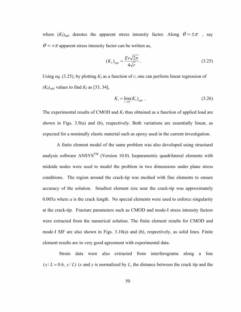
50

where (KI)app denotes the apparent stress intensity factor. Along θ π= ± , say

θ π= + apparent stress intensity factor can be written as,

2( )4I app

EvKrπ

= . (3.25)

Using eq. (3.25), by plotting KI as a function of r, one can perform linear regression of

(KI)app values to find KI as [33, 34],

1 10lim( )appr

K K→

= . (3.26)

The experimental results of CMOD and KI thus obtained as a function of applied load are

shown in Figs. 3.9(a) and (b), respectively. Both variations are essentially linear, as

expected for a nominally elastic material such as epoxy used in the current investigation.

A finite element model of the same problem was also developed using structural

analysis software ANSYSTM (Version 10.0). Isoparametric quadrilateral elements with

midside nodes were used to model the problem in two dimensions under plane stress

conditions. The region around the crack-tip was meshed with fine elements to ensure

accuracy of the solution. Smallest element size near the crack-tip was approximately

0.005a where a is the crack length. No special elements were used to enforce singularity

at the crack-tip. Fracture parameters such as CMOD and mode-I stress intensity factors

were extracted from the numerical solution. The finite element results for CMOD and

mode-I SIF are also shown in Figs. 3.10(a) and (b), respectively, as solid lines. Finite

element results are in very good agreement with experimental data.

Strain data were also extracted from interferograms along a line

( / 0.6, / )x L y L (x and y is normalized by L, the distance between the crack tip and the

51

inclusion in a crack-inclusion specimen, to be described in the next chapter) ahead of the

crack tip. A central difference scheme without any data smoothing was used to extract

strain values from interferograms. The strains were calculated as engineering strains

using the following relationship,

yy v

Nv py y

ε∂⎡ ⎤∂

= = ⎢ ⎥∂ ∂⎣ ⎦ (3.27)

where pv pitch of the virtual gratings and Ny is fringe order in the y-direction. Thus

obtained strain data was normalized by the maximum tensile strain in an uncracked

homogeneous epoxy beam strain,

2

3( )

2y beam

PSEBW

ε = , (3.28)

where P is the applied load, S, W, B are specimen dimensions (See Fig. 3.8) and E is the

Young’s modulus. The corresponding strain plot is shown in Fig. 3.11(a) as a function of

normalized y for various load levels. As expected, the strain data is relatively noisy due

to numerical differentiation and potential digitization errors, particularly close to (y/L=0)

where optical data tends to be sparse for a mode-I crack tip. The strain data from four

different load levels are shown in Fig 3.11 and the data sets overlap on each other as

expected. Also shown in the same plot is the strain variation obtained from the finite

element model along the same line showing good agreement in the overall strain

variation trends as well as magnitudes.

52

y/L-3 -2 -1 0 1 2 3

ε y / (

ε y) B

eam

0.5

0.6

0.7

0.8

0.9

1.0

1.1

533 N450 N750 N934 NFEA

x

y

m

L

Figure 3.11: Comparison of strain distribution in neat epoxy sample along line x ~3 mm (L = 5 mm, and indicated by ‘m’) from moiré data and finite element analysis.

53

CHAPTER 4

CRACK-INCLUSION INTERACTION

In this chapter experimental results from crack-inclusion interaction studies are

described. The specimens previously discussed are studied using moiré interferometry

and dominant crack opening displacements in the crack-inclusion vicinity are obtained.

Details of fracture parameters such as crack mouth opening displacements (CMOD) and

hence stress intensity factors are assessed as a function of applied load. Using measured

displacements, strains are estimated at strategic locations near the inclusion.

Experimentally obtained data will be compared to numerical results in the next chapter.

4.1 Interaction between crack and inclusion

Edge notched crack-inclusion specimens were fabricated using the method

described in Chapter 2. The notch was sharpened by razor blade insertion apparatus

discussed earlier. A schematic of a crack-inclusion specimen with and illustration of the

crack-tip coordinate system, gratings direction and loading configuration is shown in Fig.

4.1. A typical moiré fringe pattern is also shown in the region of interest. The

experimental procedure adopted is the same as the one described in Chapter 3. The

contours of crack opening displacement field (displacements along the y-direction) were

recorded as moiré interferograms (sensitivity 1.25 µm/half-fringe). Figure 4.2 shows a

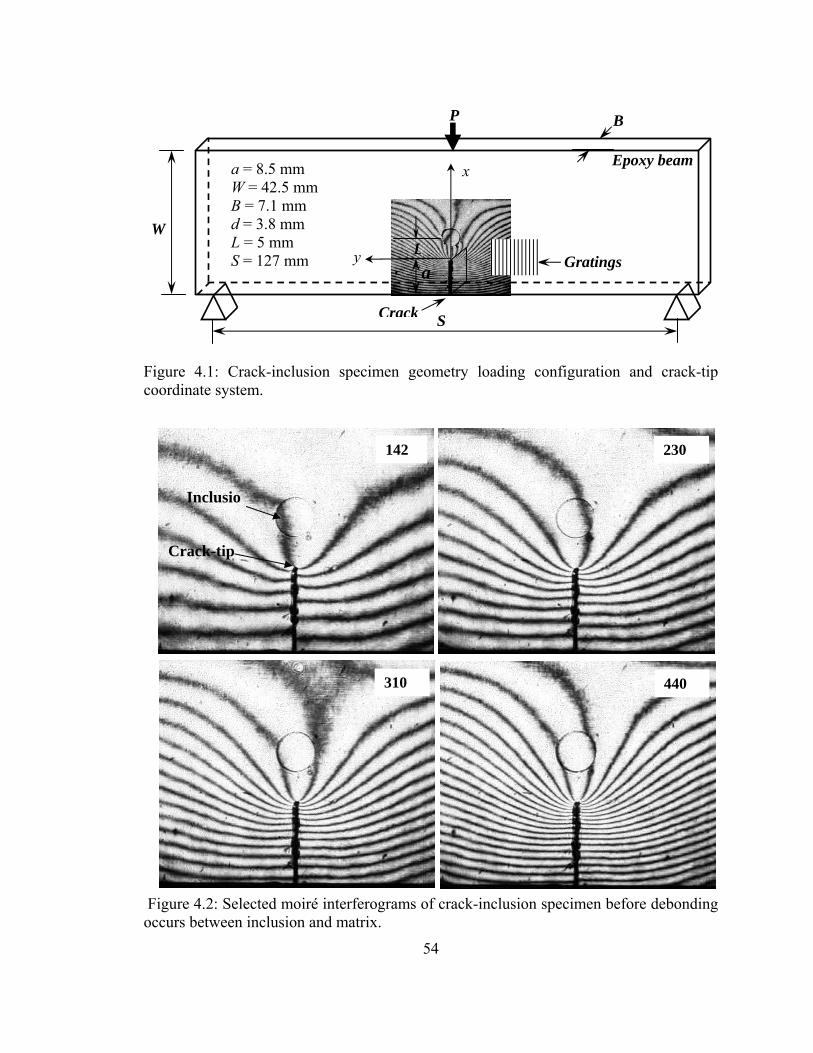
54

Figure 4.1: Crack-inclusion specimen geometry loading configuration and crack-tip coordinate system.

Figure 4.2: Selected moiré interferograms of crack-inclusion specimen before debonding occurs between inclusion and matrix.

P

x

y La

Crack


W

B

S

Epoxy beam

Gratings

310 440

142 230

Inclusion

Crack-tip

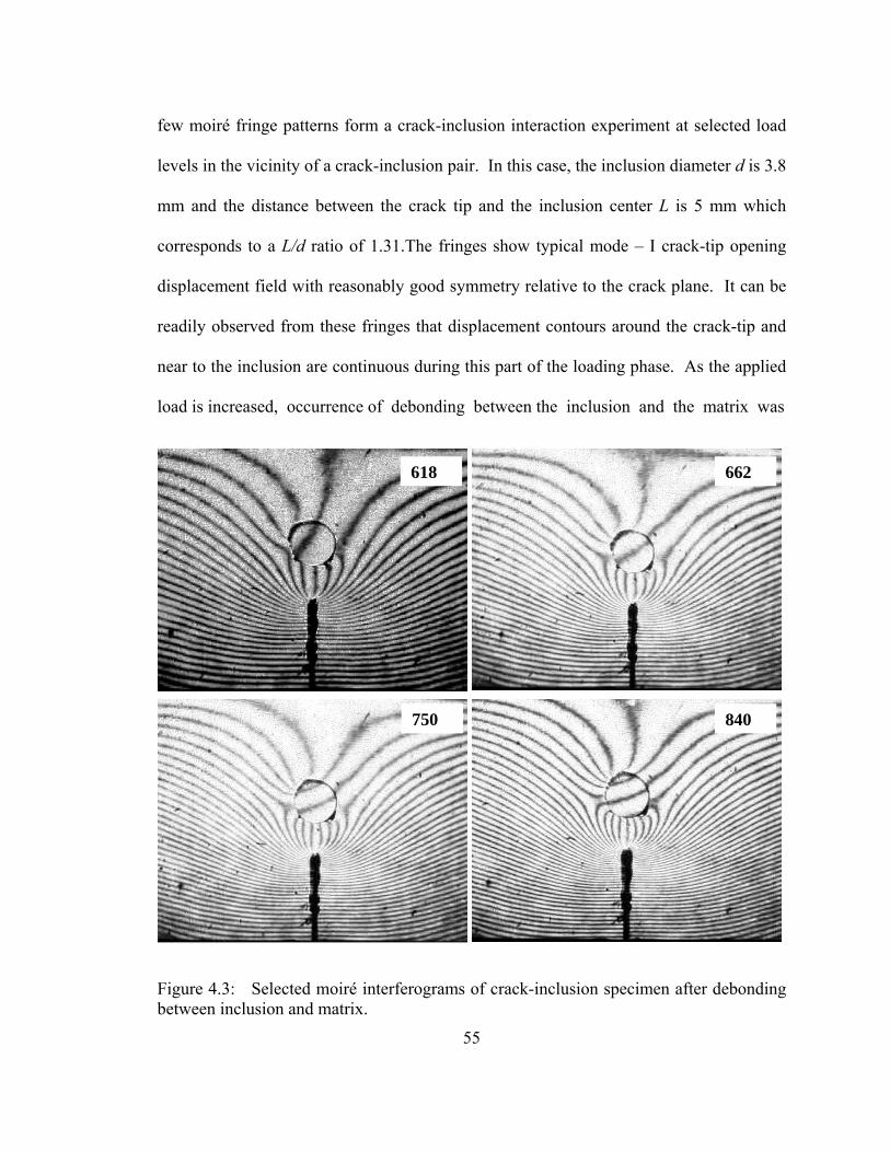
55

662 618

750 840

few moiré fringe patterns form a crack-inclusion interaction experiment at selected load

levels in the vicinity of a crack-inclusion pair. In this case, the inclusion diameter d is 3.8

mm and the distance between the crack tip and the inclusion center L is 5 mm which

corresponds to a L/d ratio of 1.31.The fringes show typical mode – I crack-tip opening

displacement field with reasonably good symmetry relative to the crack plane. It can be

readily observed from these fringes that displacement contours around the crack-tip and

near to the inclusion are continuous during this part of the loading phase. As the applied

load is increased, occurrence of debonding between the inclusion and the matrix was

Figure 4.3: Selected moiré interferograms of crack-inclusion specimen after debonding between inclusion and matrix.

56

observed and the resulting moiré interferograms from the same experiment are shown in

Fig. 4.3 for a few selected load levels. Onset of debonding can easily be detected from

successive interferograms by visual inspection of fringe pattern near the matrix-inclusion

interface. Debonding results in discontinuous fringes around the inclusion. The fringes

observed within the inclusion are parallel to each other and are equally spaced indicating

rigid rotation of the inclusion after debonding, possibly due to friction and/or incomplete

debonding between the inclusion and the matrix. A jump in the number of fringes (4-6)

around the crack was generally observed immediately following the onset of debonding.

4.2 Fracture parameters and strains

Figure 4.4: Comparison between experimentally obtained crack mouth opening displacements for the crack-inclusion and neat epoxy specimens with load.

Load (N)0 200 400 600 800

CM

OD

( µm

)

0

50

100

150

200

Neat epoxy - ExperimentInclusion - Experiment

Debond regime

57

CMOD was calculated by counting the number of fringes around the crack to the

sample edge and by using characteristic equation of moiré interferometry. The results

for the experiment are shown in Fig. 4.4. CMOD data for previously discussed neat

epoxy specimen are also shown on the same plot for comparison between the two.

Regime during the loading phase when debonding begins can be perceived by visual

inspection of interferograms and that region is highlighted in Fig. 4.4. From the graph it

can be observed that CMOD values in the crack-inclusion specimen are lower than its

neat epoxy (without inclusion) counterpart before the onset of debonding. A noticeable

Figure 4.5: Comparison of experimentally obtained variation of crack mouth compliance with applied load for crack-inclusion and neat epoxy specimens.

Load (N)

0 200 400 600 800 1000

d(C

MO

D)/d

P ( µ

m/N

)

0.18

0.20

0.22

0.24

0.26

0.28

0.30

0.32

0.34

Crack-inclusion specimenNeat epoxy specimen

Debond regime

58

jump in CMOD as a consequence of debonding is evident and hence in the post-

debonding regime where CMOD values for the crack-inclusion specimen is generally

greater than its neat epoxy counterpart. This is better evident from crack mouth

compliance (d(CMOD)/dP) values calculated from CMOD values by using a simple

central differencing scheme and are shown in Fig. 4.5. Crack mouth compliance

calculated in the same manner for the neat epoxy case is also shown on the same plot for

comparison. Evidently, the crack mouth compliance for the neat epoxy case is nearly

constant as expected for a homogeneous linear elastic material. The crack-inclusion

specimen also shows a similar behavior before the onset of debonding but with

compliance values somewhat lower than the neat epoxy case. However, the sharp rise in

Figure 4.6: Variation of mode–I SIF with load for crack-inclusion specimen.

Load (N)0 200 400 600 800 1000

KI (

MPa

-m1/

2 )

0.0

0.5

1.0

1.5

2.0

2.5

Inclusion - experimentNeat epoxy - Experiment

Debond regime

59

compliance for the crack-inclusion case is associated with occurrence of debonding

which results in a peak as it can be seen from the plot. Further, the crack mouth

compliance values are consistently higher than the ones for neat epoxy in the post-

debonding regime.

Using linear regression method described in Chapter 3, mode – I stress intensity

factors were also calculated from crack opening displacements along crack faces

(θ π= ± ) and a plot of mode-I SIF (KI) for crack-inclusion specimen is also shown in

Fig. 4.6. Again the response is generally linear as expected with the exception of a

noticeable jump in KI values when debonding occurs.

Figure 4.7: Strain field evolution along (x/L ~ 0.6, y/L) (shown by line ‘m’) during the loading phase.

y/L-3 -2 -1 0 1 2 3

ε y / (

ε y) B

eam

0.4

0.6

0.8

1.0

1.2

1.4

1.6

533 N604 N662 N916 N

x

y

m

60

Evolution of dominant strain εy along a line orthogonal to the crack and at

( / 0.6, / )x L y L ahead of the crack tip (between the crack tip and the inclusion and

nearly tangential to the inclusion) is shown in Fig. 4.7. The strains are normalized with

respect to an uncracked homogeneous beam sample of same loading configuration and

geometry as described by eq. (3.20). Load levels 533 N in the strain plot shown in Fig.

4.7 corresponds to the loading phase before debonding. Whereas, load level 604 N and

662 N corresponds to debonding regime and load level 916 N corresponds to an applied

load well after debonding. It can be seen from the plot that there is substantial

redistribution of strains ahead of the crack tip following the onset of debonding of the

inclusion from the matrix. After debonding occurs, strains close to y/L = 0 increase

drastically and attain a peak value. This can also be observed qualitatively in the

decreasing fringe spacing near the inclusion-matrix interface along y/L = 0. The contrast

between an edge cracked neat epoxy specimen (see Fig. 3.10) and crack-inclusion

specimen (see Fig. 4.7) in terms of normalized strain can be readily observed. The strains

before debonding occurs are lower in case of the crack-inclusion specimen compared to

the neat epoxy specimen due to shielding of the crack tip by the rigid inclusion. Due to

occurrence of debonding these shielding effects are compromised and strain values show

sharp increase near the inclusion-matrix interface. Noticeably, the strain redistribution is

a highly localized phenomena and strains remain unaffected beyond y/L ~ ±1. It is also

evident from Fig. 4.7 that during debonding, the strain distribution in the inclusion

vicinity is asymmetric with respect to y/L=0. This is attributed to competing debond

fronts around the inclusion.

61

4.3 Experimental repeatability

Results from two crack-inclusion interaction experiments are shown in Fig.

4.8 to address the repeatability of the crack-inclusion interaction behavior. The plot

shows variation of CMOD values for two crack-inclusion specimens. The pre-debonding

behavior is quite repeatable as can be seen from the graph whereas post-debonding

variation is within 10 µm of each other. Both experiments show occurrence of inclusion

debonding at approximately same load level and show a jump in the CMOD values. The

Figure 4.8: CMOD variation with load for two different crack-inclusion specimens.

differences in post-debonding behavior can be attributed to various reasons. The first and

the most crucial is homogeneity of bond strength that can be produced between the

inclusion and the matrix in different specimens. Due to manual treatment of glass

Load (N)0 200 400 600 800

CM

OD

( µm

)

0

50

100

150

200

Specimen - 1Specimen - 2

62

cylinders with silane some difference is expected in the bond between matrix and

inclusion in terms of the bond strength. This coupled with large stress gradient due to the

crack tip field may compound any such deviation. Another potential reason is

unavoidable errors due to experimental limitation in achievable symmetry and relative

Figure 4.9: Crack compliance variation with load for two different crack-inclusion specimens. location of crack tip and the inclusion. These result in debond front selecting a dominant

path on either side of the inclusion. However, in the post-debonding regime (well after

the completion of debonding) the two graphs are basically parallel to each other.

Experimental repeatability is better visualized by the crack mouth compliance

plots for the two experiments and are shown in Fig. 4.9. The occurrence of debonding is

evident by the steep increase in the compliance values and a distinctly different plateau

values before and after debonding.

Load (N)

0 200 400 600 800 1000

d(C

MO

D)/d

P ( µ

m/N

)

0.16

0.18

0.20

0.22

0.24

0.26

0.28

0.30

0.32

0.34

0.36

Specimen - 1Specimen - 2

63

CHAPTER 5

FINITE ELEMENT MODELING

An approach based on deactivation of stiffness for elements meeting certain

specified failure criteria has been used in a few previous works to simulate initiation and

progression of fracture in materials. Al-Ostaz and Jasiuk [35] simulated crack growth and

propagation in porous materials under uniaxial tension. They investigated crack

trajectories in perforated epoxy sheets by considering elastic strain energy and maximum

in-plane normal principal stress based failure criteria for simulating progressive failure.

Ko et. al. [36] used this method to simulate fracture in a punch problem dominated by

shear failure with a ductile-fracture criterion based on effective strain. They compared

numerical results to the ones from experiments and showed that an improved solution can

be obtained if fracture strain of the material is determined experimentally and then used

as an input in the numerical model.

This chapter describes modeling and simulation of the crack-inclusion interaction

including debonding of inclusion-matrix interface. Element stiffness deactivation method

is used in the current work to simulate onset and evolution of debonding. A finite

element model was developed in ANSYSTM [37] structural analysis environment for

static analysis of crack-inclusion interaction. ANSYS APDL (ANSYS Parametric

Design Language) macros were used for pre- and post-processing of numerical data. A

64

parametric study was performed with respect to some of the geometrical parameters of

the model.

5.1 FEA model description

Under plane stress assumptions the finite element model was defined by

specifying keypoints, joining them by lines and then creating areas in 2-D space. The

three-point-bend geometry (152mm x 42.5mm x 7.1mm), same as the one used in

experiments, was created in this manner. A symmetrically located sharp crack was

modeled by creating unmerged areas having common sides forming the two crack faces.

Isoparametric quadrilateral elements with mid-side nodes were used to create a controlled

mesh for the whole model. A representative finite element mesh used in the simulation

performed to complement experiments is shown in Fig. 5.1(a). Figure 5.2(b) shows an

enlarged view of the mesh in vicinity of the crack tip and inclusion pair. A very fine

mesh was used in the region of interest namely, in the vicinities of the crack-inclusion

pair and the inclusion-matrix interface to capture steep gradients of mechanical field

quantities. A distinct set of elements forming the interface between the inclusion and the

matrix was generated as shown in Fig. 5.1(b). This interfacial layer was modeled to have

a thickness of ~ d/100, d being the inclusion diameter. The geometrical parameters and

the coordinate systems involved are shown schematically in Fig. 5.2. In addition to the

crack tip coordinate system with origin at O, a cylindrical coordinate system with origin

O’ was also considered. In Fig. 5.2, L is the distance between the crack tip and the

center of the inclusion, d is inclusion diameter and a is crack length. Next, the

65

methodology to simulate debonding between the inclusion and the matrix during the

loading phase is discussed.

Figure 5.1: (a) Finite element mesh used for simulating crack-inclusion interaction in a three-point bend specimen (b) Enlarged view of the mesh in the vicinity of crack-tip and inclusion.

y

x

Interfacial layer of elements

Inclusion

Crack tip (b)

(a)

P

66

δCOD

θr

y

x

O

a

L

θ'O’

d

r’

Figure 5.2: Crack tip and inclusion coordinate systems.

5.2 Inclusion-matrix debonding

A criteria based on the ultimate strength of epoxy was hypothesized to simulate

debonding of the inclusion from matrix. The aforementioned interfacial elements that

constitute the bond layer were useful for this. Failure due to radial stress (relative to the

origin (O’) defined at the inclusion center) was considered for debonding of inclusion-

matrix interface. It was hypothesized that debonding occurs when radial stress attains a

fraction of the ultimate stress of the matrix material in these elements. Quasi-static

symmetric loading (P) was applied to the model with an increment of 20 N per step to

67

achieve mode – I conditions. During the loading phase, elements in this bonding layer

were monitored for radial stress with respect to the cylindrical coordinate system with

origin at the inclusion center. Post-processing was carried out at the end of each load step

and beyond a predefined value of positive radial stress to ‘kill’ (or deactivate) the bond

layer elements using ‘element death’ (EKILL) option available in ANSYS. A user

defined macro using ANSYS APDL was developed for this purpose (see, Appendix A).

To achieve the desired effect the program does not actually remove the ‘killed’ elements

in the model. Instead, elements meeting a stipulated criterion are deactivated by

multiplying their elemental stiffness by a severe reduction factor. In this work a reduction

factor of 1x10-8 was used. This prevents those deactivated elements from contributing to

the overall stiffness of the structure. That is, the respective rows and columns of the

stiffness matrix are made negligibly small without replacing them by zeros. Respective

loads in the load vector are also zeroed out but not removed from the vector. Strain and

stress values of all ‘killed’ elements are set to zero as soon as the elements are

deactivated. At the same time, large deformation effects are invoked for these elements to

achieve meaningful results. As mentioned earlier, the criteria proposed for deactivation of

an element in the bond layer is,

( )rr cr oσ βσ= , (5.1)

where (σrr)cr is the critical radial stress relative to the cylindrical coordinate system with

its axis centered at O’, σo is the strength of matrix material and β is a scalar (0 ≤ β ≤ 1).

The value of σo was used as 63 MPa for epoxy based on tensile test data shown in Fig.

4.16. A flow chart in Fig. 5.3 shows the analysis methodology described above.

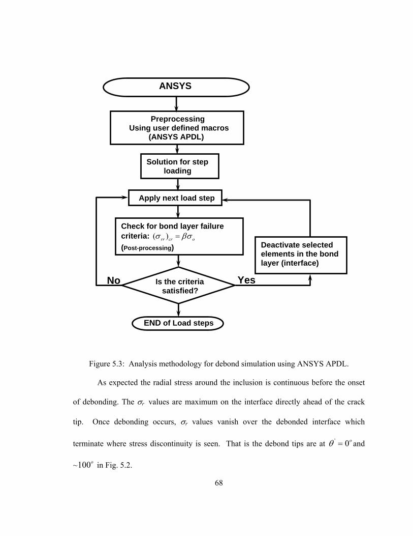
68

Figure 5.3: Analysis methodology for debond simulation using ANSYS APDL.

As expected the radial stress around the inclusion is continuous before the onset

of debonding. The σr values are maximum on the interface directly ahead of the crack

tip. Once debonding occurs, σr values vanish over the debonded interface which

terminate where stress discontinuity is seen. That is the debond tips are at ' 0oθ = and

~100o in Fig. 5.2.

ANSYS

Preprocessing Using user defined macros (ANSYS APDL)

Solution for step loading

Apply next load step

Check for bond layer failure criteria: ( )rr cr oσ βσ= (Post-processing)

Is the criteria satisfied?

Deactivate selected elements in the bond layer (interface)

YesNo

END of Load steps

69

Figure 5.4: (a) Variation of radial stress variation around the inclusion for b = 0.12 (applied load P is normalized by Po, the load corresponding to tensile failure of an uncracked neat epoxy beam).(b) CMOD variation for various β values (eq. (5.1)) used in finite element simulations and comparison with experimental results. (L/d = 1.31, d = 4 mm)

Load (N)

0 200 400 600 800

CM

OD

( µm

)

0

50

100

150

200

Experimentβ=0.079β=0.127β=0.143β=0.206β=0.301

(b)

θo (deg.)

-150 -100 -50 0 50 100 150

σ r (M

Pa)

-10

-8

-6

-4

-2

0

2

4

6

8

10

Before debonding (P/Po = 0.12)After debonding (P/Po = 0.20)β = 0.14

(a)

70

5.3 Effect of β on debonding

Figure 5.4(a) shows the variation of radial stress along the bond layer before and

well after the occurrence of debonding. After an element meets the debond criteria its

strain and hence stress are set to zero. Various values of β were considered for

simulating debonding. A plot of CMOD as a function of applied load for various values

of β in eq. (5.1) is shown in Fig. 5.4(b). Each plot shows a linear variation of CMOD

with load until the onset of debonding. Post-debonding regimes have noticeably different

slopes when compared to pre-debonding ones. A transition zone in between the two can

also be identified. On the same plot, experimentally obtained CMOD values from moiré

interferometry are also shown. A value of β = 0.14 in eq. (5.1) resulted in a good

agreement with experimental observations. A lower or a higher value of β relative to this

Figure 5.5: Crack mouth compliance comparison between experimental and FEA data. Load (N)

0 200 400 600 800

d(C

MO

D)/d

P ( µ

m/N

)

0.18

0.20

0.22

0.24

0.26

0.28

0.30

0.32

0.34

0.36

ExperimentFEA

Debonding regime

71

Figure 5.6: Strain field evolution along (x ~ 3 mm, y) (shown by line ‘m’) for (a) pre-debonding and (b) post-debonding stages.

y/L-3 -2 -1 0 1 2 3

ε y /

( εy)

Bea

m

0.0

0.2

0.4

0.6

0.8

1.0

1.2

1.4

1.6

1.8

ExperimentFEA x

y

m

(a)

y/L-3 -2 -1 0 1 2 3

ε y /

( εy)

Bea

m

0.0

0.2

0.4

0.6

0.8

1.0

1.2

1.4

1.6

1.8

ExperimentFEA x

y

m

(b)

72

value results in initiation of debonding at lower or higher loads, respectively, as

expected. Evidently, following debonding, all graphs coincide with each other.

Next crack mouth compliance (d(CMOD)/dP) was calculated by differentiating

CMOD data obtained from FE simulation. A central difference scheme was used to

compute compliance and the result is shown in Fig. 5.5 indicated by a solid line. On the

same plot the experimentally observed crack mouth compliance values are also shown.

An excellent agreement between the finite element model and experimental data is

readily evident from this graph. A sudden increase in compliance occurs following the

onset of debonding. A relatively higher plateau in compliance values in the post-

debonding regime compared to the ones from pre-debonding regime can be readily

observed.

Next strain evolution along a line (x/L ~ 0.6, y/L) (shown by ‘m’ in Fig. 5.6) near

the inclusion-matrix interface from the finite element model are discussed. The strains in

Fig. 5.6 are normalized with respect to maximum beam strains, as described in Chapter 3

and the plots are shown for pre- and post-debonding regimes in Figs. 5.6(a) and (b)

respectively. The experimental data (from Chapter 4 (Fig. 4.7)) is also shown on the same

plot for comparison. The strain values from FEA model are in good agreement with

experimental data and these strain plots show a behavior similar to the one observed in

experiments. The difference between experimental and finite element strain values closer

to the inclusion-matrix interface is not completely unexpected considering the

asymmetries entering the model (see Fig. 5.4(a)) after the occurrence of inclusion-matrix

73

(b)

(a)

(360 N)

(840 N)

Figure 5.7: Crack opening displacement field from finite element analysis showing perturbed displacement contours in the crack-inclusion vicinity. (a) Before debonding (b) After debonding. Contours levels are approximately same as the experimental ones. (a = 8.5 mm, d = 4mm, L/d = 1.31, β = 0.14).

74

debonding. Further, strain differences are due to possible digitization and differentiation

errors as noted earlier.

After the onset of debonding a qualitatively similar progression of the debond

front as in experiments was observed in finite element simulations. Also the fringe

spacing in the vicinity of crack-inclusion was observed to decrease in post-debonding

regime which is evident from the strain plot as a steep increase in Fig. 5.6(b).

Representative plots of opening displacement fields from the finite element analysis in

Figure 5.8: Energy release rate variation with applied load.

vicinity the of crack-inclusion pair, before and after debonding, are shown in Fig. 5.7.

Here the contour levels are same as the one in moiré interferometry. Qualitative

agreement between experimentally recorded opening displacements fields (Figs. 4.2 and

Load (N)

0 200 400 600 800 1000

ERR

(N/m

)

0

200

400

600

800

1000

1200

1400

1600

1800

ExperimentFEA

75

Figure 5.9: Normal Strain evolution along line ‘m’ (a) εx (b) εy.

y/L-2 -1 0 1 2

ε y/εm

ax-b

eam

0.0

0.2

0.4

0.6

0.8

1.0

1.2

1.4

1.6

1.8

Before debondingAfter debonding

x

y

m

(b)

y/L

-2 -1 0 1 2

ε x/ ε

max

-bea

m

-0.6

-0.4

-0.2

0.0

0.2

0.4

0.6

0.8

1.0

1.2

After debondingBefore debonding

x

y

m

(a)

76

Figure 5.10: Evolution of (a) Shear strain εxy (b) Von-Mises stess along line ‘m’.

y/L

-2 -1 0 1 2

ε xy/ ε

max

-bea

m

-2.0

-1.5

-1.0

-0.5

0.0

0.5

1.0

1.5

2.0


x

y

m

(a)

y/L

-2 -1 0 1 2

σ von_

mis

es/ σ

max

-bea

m

0.6

0.8

1.0

1.2

1.4

1.6

1.8

2.0


x

y

m

(b)

77

4.3) and the ones from finite element analysis is readily evident. Discontinuous fringes

around the inclusion periphery in the interferograms shown in Figs. 4.2 and 4.3 are also

evident in Fig. 5.7. Thus the overall crack tip behavior in terms of crack opening

displacements is preserved in these simulations.

A user-defined macro was used to extract mode – I stress intensity factors (KI)

from the finite element model. Linear regression methods using crack opening

displacement alongθ π= ± , as described in Chapter 3 was used and subsequently

Energy Release Rates (ERR) were calculated as,

2IKERR G

E= = for plane stress (5.2)

where E is the Young’s modulus of the matrix material. A good agreement can be seen

between experiments and simulations from the results plotted in Fig. 5.8.

Normal strains (εx) and (εy) shear strains (εxy) were also extracted along (x/L ~ 0.6,

y/L) (shown by line ‘m’) from the finite element model and are shown in Figs. 5.9 and

5.10(a). (For completeness a plot of normal strain (εy) along ‘m’ is reproduced in Fig.

5.9(b)). All strain components also shows drastic increase in the vicinity of the inclusion

after debonding whereas beyond y/L = ±1 the values are almost unaffected suggesting a

highly localized phenomena. Figure 5.10(b) shows a plot of von-Mises stresses along the

same line for the pre- and post-debonding regimes.

5.4 Convergence study

To ensure the accuracy of the results a convergence study was performed. As

described earlier the model is comprised of a distinct set of elements along the interface

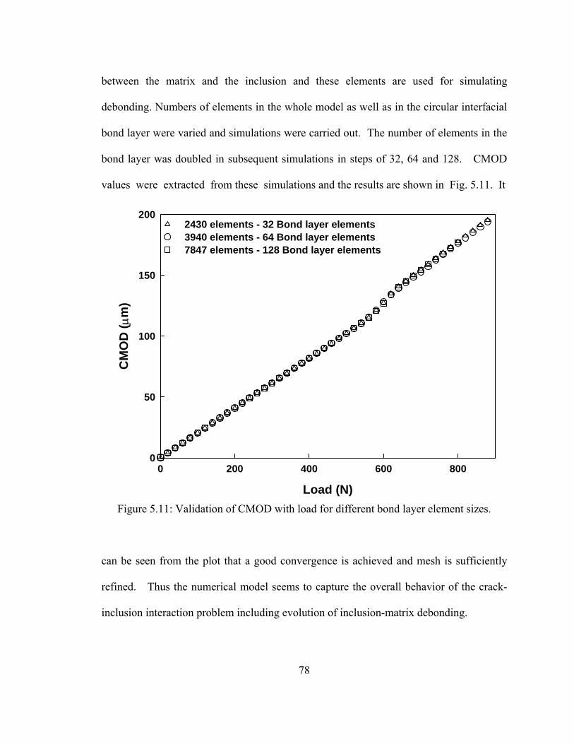
78

between the matrix and the inclusion and these elements are used for simulating

debonding. Numbers of elements in the whole model as well as in the circular interfacial

bond layer were varied and simulations were carried out. The number of elements in the

bond layer was doubled in subsequent simulations in steps of 32, 64 and 128. CMOD

values were extracted from these simulations and the results are shown in Fig. 5.11. It

Figure 5.11: Validation of CMOD with load for different bond layer element sizes.

can be seen from the plot that a good convergence is achieved and mesh is sufficiently

refined. Thus the numerical model seems to capture the overall behavior of the crack-

inclusion interaction problem including evolution of inclusion-matrix debonding.

Load (N)

0 200 400 600 800

CM

OD

( µm

)

0

50

100

150

2002430 elements - 32 Bond layer elements3940 elements - 64 Bond layer elements7847 elements - 128 Bond layer elements

79

5.5 Parametric study

5.5.1 Constant L/d ratio: Effect of inclusion size

A parametric study was carried out for different L/d ratios using the finite element

model for the edge cracked geometry loaded in symmetric three-point bend

configuration. In all simulations β = 0.14 for which good agreement between

experiments and simulations were observed is used. The effect of inclusion size was

studied for a constant L/d ratio with respective L and d values shown in Table 5.1. Here

L is the distance between the crack tip and inclusion center and d is the diameter of the

inclusion. A bonding layer thickness (tb) of d/100 was used in each of these simulations.

The model parameters used for these are listed in Table 5.1.

The plot of variation of CMOD with applied load is shown in Fig. 5.12 for a

constant L/d ratio of 1.31 with different diameters of inclusions. The applied load in

these plots is normalized by Po, the load at which a neat epoxy beam would fail in tension

based on ultimate strength of epoxy (σo). Po is calculated by using equation,

22

3o

oBWPS

σ= (5.3)

where B is the thickness, W is the height of the beam and S is span. The value of Po was

thus calculated as (4241 N) as failure load of an uncracked neat epoxy beam. For these

simulations parameter L was varied with respect to the inclusion diameter d to achieve a

constant L/d ratio. A delayed debonding was observed for larger inclusions whereas

smaller inclusions get debonded from the matrix at much lower loads, as seen from plot

in Fig 5.12. This can be visualized better from the crack mouth compliance

(d(CMOD)/dP) calculated by differencing CMOD values with respect to the applied load,

80

Table 5.1: Geometric parameters used for study with a constant L/d ratio.

Figure 5.12: CMOD variation with load for L/d ratio of 1.31.

# L (mm) d (mm) L/d tb (mm) 1 0.655 0.5 1.31 0.006 2 1.31 1 1.31 0.01 3 2.62 2 1.31 0.02 4 5 3.8 1.31 0.05 5 6.55 5 1.31 0.05 6 7.86 6 1.31 0.06 7 9.17 7 1.31 0.07 8 10.48 8 1.31 0.08

Load (N)

0 200 400 600 800 1000 1200

CM

OD

( µm

)

0

50

100

150

200

250

300

d = 0.05 mmd = 1 mmd = 2 mmd = 3.8 mmd = 5 mmd = 6 mmd = 7 mmd = 8 mm

81

Figure 5.13:Variation of crack mouth compliance with respect to applied load.(L/d=1.31)

Figure 5.14: Crack mouth compliance values for different inclusion diameters (L/d = 1.31).

P/Po

0.0 0.1 0.2 0.3

d(C

MO

D)/d

P ( µ

m/N

)

0.20

0.22

0.24

0.26

0.28

0.30

0.32

0.34

0.36

d/a = 0.0058d/a = 0.117d/a = 0.235d/a = 0.447d/a = 0.588d/a = 0.705d/a = 0.823d/a = 0.941

d/a 0.0 0.2 0.4 0.6 0.8 1.0

d(C

MO

D)/d

P ( µ

m/N

)

0.18

0.20

0.22

0.24

0.26

0.28

0.30

0.32

0.34

0.36

Before debondingAfter debondingPeak Value

82

and are shown in Figure 5.13. Each compliance plot shows different steady state values

before and after debonding. In this context it is worth noting that crack mouth

compliance for a cracked neat (without any inclusion) epoxy beam is 0.21 µm/N. At the

onset of debonding compliance shows a jump and attains distinctly different maximum

value in each case. The compliance values before debonding, after debonding as well as

the maxima during the loading phase are shown in Fig. 5.14. Maximum values increase

until a d/a value of 0.6 but drop with further increase in d/a. Though the physical

Figure 5.15: Energy release rates for different diameter inclusions (L/d = 1.31).

significance of these maximum values is unclear at the moment, further investigation

would likely shed more light on the issue.

P/Po

0.00 0.05 0.10 0.15 0.20 0.25 0.30

Gin

clus

ion/G

neat

epo

xy

0.90

0.95

1.00

1.05

1.10

1.15

1.20d/a = 0.0058d/a = 0.117d/a = 0.235d/a = 0.447d/a = 0.588d/a = 0.705d/a = 0.823d/a = 0.941

83

Normalized energy release rates (ERR) were also calculated from the simulations

as described by eq. 5.2 and corresponding plots of the same is shown in Fig. 5.14. A

behavior similar to the one observed from crack mouth compliance values is observed.

The normalization was done with respect to the energy release rates associated with a

same geometry (edge cracked three-point bend) neat epoxy specimen at the same load

level (Gneat epoxy) calculated as,

2

epoxy

( )I neatneat epoxy

KG

E= (5.4)

Opening strains (εy) were extracted from these simulations involving a constant

L/d ratio of 1.31. Figures 5.16(a) and (b) show the plots of normalized εy in pre- and

post-debonding regimes respectively. A normalized load of P/Po= 0.023 is considered

for the pre-debonding regime plots which corresponds to a load level well before

debonding. For post-debonding regime the normalized load value is P/Po= 0.30 which

corresponds to a load level after debonding. Here Po (= 4241 N) is the load value

corresponding to failure of a homogeneous uncracked beam based on failure strength of

matrix (epoxy) material. The increasing shielding effect is evident here in the pre-

debonding regime (Fig. 5.16(a)) as inclusion size increases from lower values of strains

near matrix-inclusion interface for larger size inclusions. In post-debonding regime also

the same trend is observed for larger size inclusions as seen from Fig. 5.16(b).

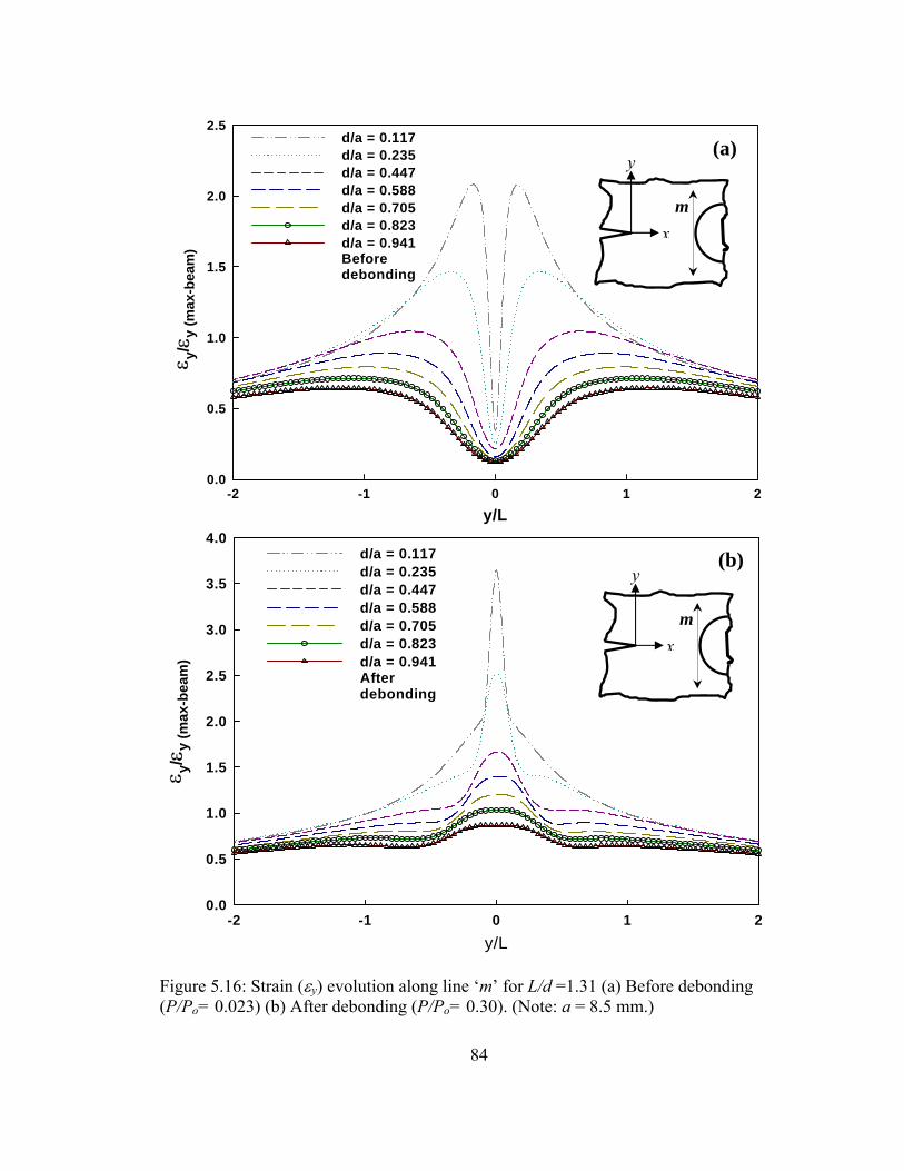
84

Figure 5.16: Strain (εy) evolution along line ‘m’ for L/d =1.31 (a) Before debonding (P/Po= 0.023) (b) After debonding (P/Po= 0.30). (Note: a = 8.5 mm.)

y/L-2 -1 0 1 2

ε y/ε y

(max

-bea

m)

0.0

0.5

1.0

1.5

2.0

2.5d/a = 0.117d/a = 0.235d/a = 0.447d/a = 0.588d/a = 0.705d/a = 0.823d/a = 0.941Before debonding

y/L-2 -1 0 1 2

ε y/ε y

(max

-bea

m)

0.0

0.5

1.0

1.5

2.0

2.5

3.0

3.5

4.0d/a = 0.117d/a = 0.235d/a = 0.447d/a = 0.588d/a = 0.705d/a = 0.823d/a = 0.941Afterdebonding

x

y

m

x

y

m

(a)

(b)

85

5.5.2 Varying L/d ratio: Crack-inclusion proximity effect

Next, the L/d ratio was varied to examine the effect of inclusion proximity with

the crack tip and its impact on overall behavior of the problem. In this case inclusion size

(d) was varied whereas the distance between the crack tip and inclusion center L was kept

Table 5.2: Geometric parameters used for studying effect of L/d ratio.

Figure 5.17: Variation of crack mouth opening displacement with the applied load.

# L (mm) d (mm) L/d tb (mm) 1 5 1 5 0.01 2 5 2 2.5 0.02 3 5 3.8 1.25 0.04 4 5 5 1 0.05 5 5 6 0.83 0.06 6 5 7 0.71 0.07 7 5 8 0.63 0.08

Load (N)

0 200 400 600 800 1000 1200

CM

OD

( µm

)

0

100

200

300

400

d = 1 mmd = 2 mmd = 3.8 mmd = 5 mmd = 6 mmd = 7 mmd = 8 mm

86

constant. The values of parameters L and d used in this set of simulations are tabulated in

Table 5.2.

The CMOD values for this study are shown in Fig. 5.17. It can be seen from the

plots that as the L/d ratio decreases the debonding occurs much earlier. Also, the CMOD

values are lower for higher L/d before debonding whereas after debonding the trend is

reversed. The inclusions nearer to the crack-tip show variation of CMOD with noticeably

higher slopes. The compliance plots obtained from Fig. 5.17 shown in Fig. 5.18

demonstrate this more distinctly. It can be seen that the compliance values before and

after debonding show opposite trends. The peak compliance values attained along with

the steady state values before and well after the occurrence of debonding are shown in

Fig. 5.19 for various L/d ratios. Peak compliance values show increasing trend as the L/d

Figure 5.18: Variation of crack mouth compliance with the applied load.

P/Po

0.00 0.05 0.10 0.15 0.20 0.25 0.30

d(C

MO

D)/d

P ( µ

m/N

)

0.2

0.3

0.4

0.5

0.6

0.7

d/a = 0.117, L/d = 5d/a = 0.235, L/d = 2.5d/a = 0.447, L/d = 1.31d/a = 0.588, L/d = 1d/a = 0.705, L/d = 0.83d/a = 0.823, L/d = 0.71d/a = 0.941, L/d = 0.63

87

ratio decreases (when the distance between the crack tip and the inclusion center (L) is

constant). The values associated pre-debonding regime shows a decreasing trend with

decrease in the L/d ratio whereas after debonding the trend is reversed. For this case (L/d

varying), normalized energy release rates (or, crack driving force) are shown in Figure

5.20. In each case, shielding effect is evident before the occurrence of debonding as the

L/d ratio increases whereas after debonding the energy release rates shows steep increase

and settles at a higher value for larger L/d ratios. From L/d = 5 to L/d = 0.625 the

normalized value of energy release rate is increased approximately 2.5 times as evident

form the plot. That is, an inclusion which is much closer to the crack tip

Figure 5.19: Steady state and maximum values of crack mouth compliance with variation of L/d ratio.

L/d

0 1 2 3 4 5

d(C

MO

D)/d

P ( µ

m/N

)

0.1

0.2

0.3

0.4

0.5

0.6

0.7

Before debondingAfter debondingPeak Value

88

Figure 5.20: Energy release rates for different L/d ratios. when debonds increases the crack driving force (by a factor of ~ 2.5 in this study) as well

as crack mouth compliance when compared to the one farther away.

For the case of varying L/d ratio the opening strains (εy) were extracted and the

corresponding plots of strains along line ‘m’ are shown in Figs. 5.21(a) and 5.21(b). The

corresponding load levels for each of these plots are kept same as Figs. 5.16(a) and (b)

respectively. As L/d ratio increases εy values shows increasing trend in the vicinity of the

inclusion-matrix interface in the pre-debonding regime (Fig. 5.21(a)). Figure 5.21(a)

shows a slight decrease in εy values for L/d ratio larger than 0.71. Whereas εy values

show a monotonic increase in the post debonding regime with increase in the L/d ratio as

seen from Fig. 5.21(b).

P/Po

0.00 0.05 0.10 0.15 0.20 0.25 0.30

Gin

clus

ion/

Gne

at e

poxy

0.5

1.0

1.5

2.0

2.5

3.0

L/d = 5L/d = 2.5L/d = 1.31L/d = 1L/d = 0.83L/d = 0.71L/d = 0.63

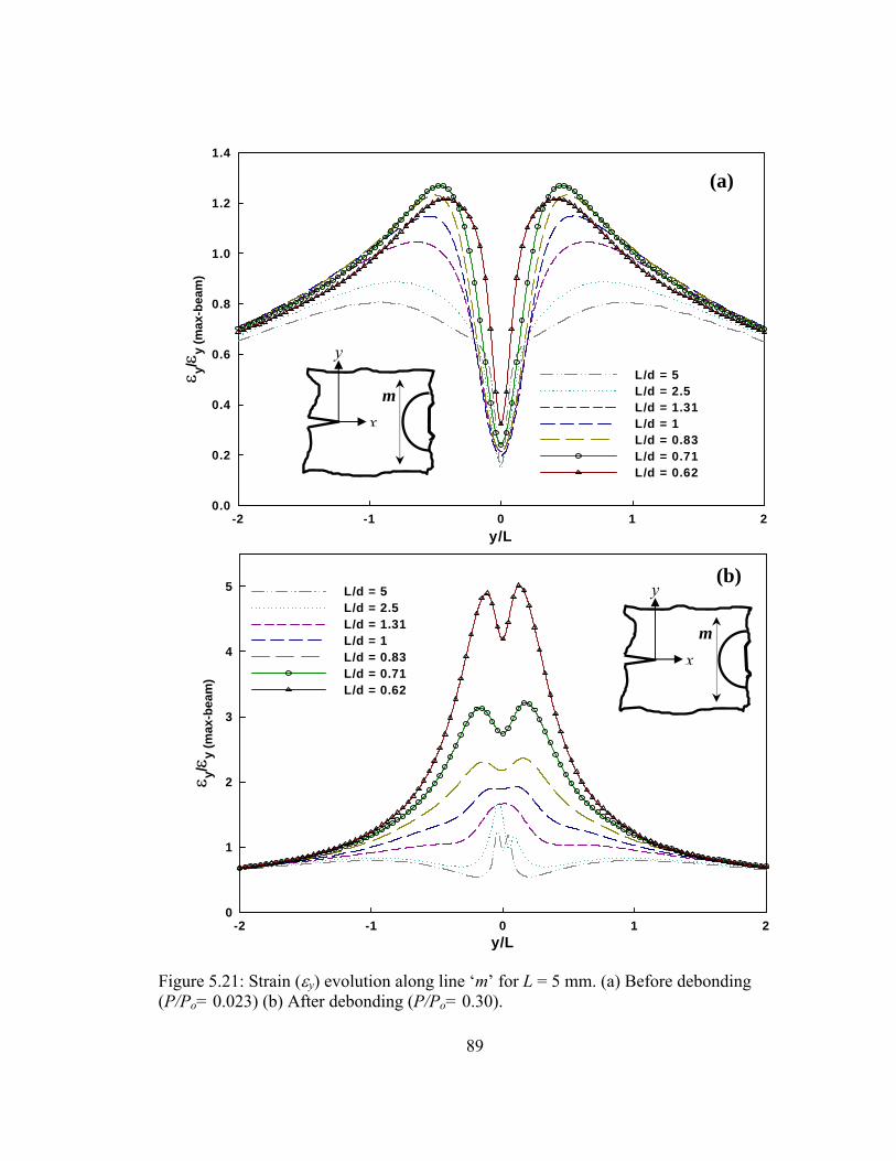
89

Figure 5.21: Strain (εy) evolution along line ‘m’ for L = 5 mm. (a) Before debonding (P/Po= 0.023) (b) After debonding (P/Po= 0.30).

y/L-2 -1 0 1 2

ε y/ε y

(max

-bea

m)

0

1

2

3

4

5 L/d = 5L/d = 2.5L/d = 1.31L/d = 1L/d = 0.83L/d = 0.71L/d = 0.62

y/L-2 -1 0 1 2

ε y/ε y

(max

-bea

m)

0.0

0.2

0.4

0.6

0.8

1.0

1.2

1.4

L/d = 5L/d = 2.5L/d = 1.31L/d = 1L/d = 0.83L/d = 0.71L/d = 0.62

x

y

m

x

y

m

(a)

(b)

90

5.6 Estimation of glass-epoxy interface strength To provide a physical interpretation for the value of β = 0.14 in eq. (5.1) that

provided good agreement with experimental CMOD variation, nominal interfacial

strength between epoxy and glass was measured. This was done using T-shaped tension

specimens shown schematically in Fig. 5.22. Clean surface of a rectangular glass bar

(75mm x 25mm x 6.6mm) that has the surface finish same as that of the glass inclusion

was treated with silane and dried at room temperature for 24 hours. Silicone rubber

molds were prepared to cast epoxy (70mm x 21mm x 7.1mm) stems on the glass surface.

Figure 5.22: Schematic of specimens and loading configuration used for estimating glass-epoxy bond strength. (Note: All dimensions are in mm.)

Side view Front view

Glass

Epoxy

70 21

7

25 75

91

Figure 5.23: Silicone rubber molds cast on a flat surface.

Silicone molds thus prepared are shown in Fig 5.23. These molds were separated from

the casting surface after they were cured and the epoxy bar used to cast the mold was

pulled out. After proper alignment of the mold over the treated glass surface liquid epoxy

was again poured into the mold and allowed to cure for 72 hours at room temperature.

Casting epoxy in this way allowed preparing bond between epoxy and glass in a manner

similar to the one that exists between the inclusion surface and the matrix in crack-

inclusion specimens. The specimens were tested in an INSTRON 4465 testing machine

and load data were collected until glass-epoxy interface failed. A photograph of the test

setup is shown in Fig. 5.24. Brittle failures of the glass-epoxy interfaces were observed

and average failure stresses for several samples tested are reported in Table – 5.3.

Silicone

Epoxy stub

Mold

92

Figure 5.24: Experimental setup for glass-epoxy interfacial strength measurement.

Table 5.3: Glass-epoxy interfacial failure strength data.

Specimen # Failure stress (MPa)

1 7.46

2 10.39

3 9.90

Average interfacial failure strength = 9.25 MPa

Epoxy

Glass

93

The average value of the interface strength was estimated as 9±1 MPa.

Interestingly, (σrr)cr value in eq. (7) that produced good agreement (=βσo) with moiré

data is within 5% of the interfacial strength between epoxy and glass. This further

validates the proposed model used in the FE simulations.

It should also be noted that a few experiments on T-specimens prepared without

silane treatment were carried out. The resulting weaker interface showed an average

interfacial strength of 3 ± 1 MPa, nearly a third of the one when glass was treat with

silane.

94

CHAPTER 6

CONCLUSIONS

In this work a stationary crack interacting with a relatively stiff inclusion and the

resulting debonding of the inclusion from the matrix were studied experimentally and

numerically. Three-point bend (TPB) epoxy specimens with edge cracks and solid

cylindrical glass inclusion were examined. The full-field technique of moiré

interferometry was used to map deformations in the crack-inclusion vicinity. The

experimental novelty here includes development of microelectronics fabrication based

methods for printing specimen gratings using two approaches namely, (1) Direct transfer

of aluminum coated gratings from a silicon wafer master and (2) Indirect transfer of

gratings using silicone rubber submasters. High quality grating profiles were achieved

using these two methods. A moiré interferometer was developed and used to acquire high

quality interferograms. An optical resolution of 1.25 µm/half-fringe was successfully

achieved and results were benchmarked using a cracked TPB specimen made of neat

epoxy.

Next, crack-inclusion specimens were fabricated and deformations were mapped

near crack-inclusion vicinity during monotonically increasing load. The occurrence of

debonding between the matrix and the inclusion was successfully identified during the

loading phase. Pre- and post-debond deformation fields show localized differences ahead

95

of the crack tip and near the inclusion. The fringe contours clearly show discontinuity at

the matrix-inclusion interface and observable asymmetry in displacements around the

inclusion due to selective propagation of the debond front. A change in the crack mouth

compliance was clearly evident at the onset of debonding. Substantial differences in

terms of dominant strains obtained by differentiating the optical data were also evident

when pre- and post-debond stages were compared. Opening strain values showed

noticeable increase in the vicinity of the crack tip and the inclusion near to inclusion-

matrix interface after debonding whereas far field strains remain relatively unaffected.

A finite element model was developed to capture the major experimental

observations. This was achieved by implementing a inclusion-matrix debond criteria

based on an interfacial layer of elements attaining a fraction of the ultimate strength of

the epoxy matrix. The debonding process was simulated by deactivating stiffness of

interfacial layer of elements by a user-defined macro in ANSYS structural analysis

environment. Various bond strengths were used as a fraction of the ultimate strength of

the matrix material and the finite element model was validated against the experimental

data. The displacement and strain fields were compared successfully with experimental

results. A follow up experiment to measure apparent interfacial strength of glass-epoxy

suggested that inclusion debonded when radial stress at a location on the interface

reached the interfacial strength of the interface.

A parametric study was undertaken using the finite element model. Mainly two

different scenarios were studied: (1) Inclusion size effect (constant L/d ratio) and (2)

Inclusion proximity effect (varying L/d ratio). Fracture parameters such as crack mouth

opening displacement (CMOD) and energy release rates were calculated using the finite

96

element model. At a constant L/d ratio the larger size inclusions show delayed debonding.

Also the peak value of crack mouth compliance attained during debonding was observed

to increase until a d/a ratio of approximately 0.58 whereas further increase showed a

decreasing trend. The study of varying L/d ratio (with constant L) showed that a larger

inclusion shields the crack tip more before debonding. However, a larger inclusion

debonds at a lower load and results in higher crack mouth compliance than the smaller

size inclusion upon debonding. Energy release rate for a larger inclusion (L/d = 0.63)

showed a higher value (~ 2.5 times) than smaller (L/d = 5) inclusion at a fixed value of L

(= 5 mm) in post-debonding regime in this study.

97

BIBLIOGRAPHY

1. Jones R. M., Mechanics of composite materials, Second edition, Taylor and

Francis, Inc., 1999. (ISBN: 1-56032-712-X)

2. Marple B. S. and Boulanger J., Graded casting of materials with continuous gradients, Journal of American Ceramic Society., 77(10), pp.2747, 1994.

3. Fukui Y., Takashima K. and Ponton C. B., Measurement of Young’s modulus

and internal friction of an in-situ Al-Al3Ni functionally gradient material, Journal of Materials Science, 29, pp.2281, 1994.

4. Abboud J. H., Rawlings R. D. and West D. R. F., Functionally graded nickel-

aluminide and iron-aluminide coatings produced via laser cladding, Material Science and Technology., 10, pp.414, 1994.

5. Sampath S., Gausert R. and Herman H., Plasma-spray forming ceramics and

layered composites, Journal of Metals. 47, pp.30, 1995. 6. Butcher R. J., Rousseau C. –E., Tippur H. V., A functionally graded particulate

composite: Preparation, measurements and failure analysis, Acta Materilia, 47(1), pp.259-268, 1999.

7. Rousseau C. –E., Tippur H. V., Compositionally graded materials with cracks

normal to the elastic gradient. , Acta Materilia, 48, pp.4021-4033, 2000. 8. Kirugulige M. S., Kitey R., Tippur H. V., Dynamic fracture behavior of model

sandwich structures with functionally graded core: a feasibility study, Composite Science and Technology., 65, pp.1052-1068, 2005.

9. Tamate O., “The effect of a circular Inclusion on the stress around a line crack in

a sheet under tension,” International Journal of Fracture Mechanics., 4, pp.275-266, 1968.

10. Atkinson C., “The interaction between a crack and an inclusion, “International

Journal of Engineering Sciences, 10, pp.127-136, 1972.

98

11. Erdogan F., Gupta G. D. and Ratwani M., “Interaction between a circular inclusion and an arbitrarily oriented crack,” Journal of Applied Mechanics, 41, pp.1007-1013, 1974.

12. Gduotos E.E., Interaction effects between a crack and a circular inclusion, Fibre

Science and Technology, 15(1), pp.27-40, 1981. 13. Gduotos E.E., Stable Crack Growth of a Crack Interacting with a Circular

Inclusion, Theoretical and Applied Fracture Mechanics, 3(2), pp.141-150, 1985. 14. Kunin I., Gommerstadt B., On Elastic Crack-Inclusion Interaction, International

Journal of Solids and Structures, 21(7), pp.757-766, 1985. 15. Hasebe N., Okumura M., Nakumura T., Stress-Analysis of a debonding and a

crack Around a Circular Rigid Inclusion, International Journal of Fracture., 32(3), pp.169-183,Nov 1986.

16. Patton E. M., Santare M. H., The effect of a rigid elliptical inclusion on a straight

crack, International Journal of Fracture, 46, pp.71-79, 1990. 17. Li R. and Chudnovsky A., Energy analysis of crack interaction with an elastic

inclusion, International Journal of Fracture, 63, pp.247-261, 1993. 18. Li R., and Chudnovsky A., The stress intensity factor Green’s function for a

crack interacting with a circular inclusion, International Journal of Fracture,67, pp.169-177, 1994.

19. Bush M., The interaction between a crack and a particle cluster, International

Journal of Fracture, 88, pp.215-232, 1997. 20. Knight M. G., Wrobel L. C., Henshall J. L., De Lacerda L. A., A study of the

interaction between a propagating crack and an uncoated/coated elastic inclusion using BE technique, International Journal of Fracture., 114, pp.47-61, 2002.

21. Kitey R., Phan A. V. Tippur H. V., Kaplan T., Modeling of crack growth through

particulate clusters in brittle matrix by symmetric-Galerkin boundary element method, International Journal of Fracture, 2005 (Article in press).

22. Kitey R., Microstructural effects on Fracture behavior of particulate composites:

Investigation of toughening mechanism using optical and boundary element methods, Doctoral thesis and dissertation, Auburn University, 2006.

23. O’Toole B. J., Santare M. H., Photoelastic Investigation of Crack-inclusion

Interaction, Experimental Mechanics, 30(3), pp.253-257, 1990.

99

24. Li R., Wu S., Ivanova E., Chudnovsky A., Sehaobish K., and Bosnyak C.P., Finite Element Model and Experimental Analysis of Crack-Inclusion Interaction, Journal of Applied Polymer Sciences, 50, pp.1233-1238, 1993.

25. Easley T. C., Faber K. T., Shah S. P., Moiré interferometry analysis of fiber debonding, Journal of Engineering Mechanics, 127, pp.625-629, 2001. 26. Jaeger R. C., Introduction to Microelectronic Fabrication, Second Edition,

Vol. 5, Prentice Hall, NJ, 2002.

27. Post D., Han B., Ifju P., High sensitivity moiré, Springer–Verlag, New York, 1994. 28. Post D. and Baracat W. A., High-sensitivity moiré interferometry – A simplified approach, Exp. Mech., 21(3), pp100-104, 1981.

29. Krishnamoorthy H., Estimation of fracture parameters in solder-copper joints using moiré interferometry, Master’s thesis, Auburn University, 1997. 30. Tippur H., Optical methods in mechanics, Lecture notes, Auburn University, Spring 2005. 31. Chiang F. P., Doyle J. F., Phillips J. W., Manual on Experimental Stress Analysis, Society of Experimental Mechanics, Connecticut, 1989.

32. Williams M. L., On the stress distribution at the base of a stationary crack, Journal of Applied Mechanics, 24, pp.109-104, 1957. 33. Rousseau C. –E., Tippur H. V., Influence of elastic gradient profiles on dynamically loaded functionally graded materials: Cracks along the gradient, International Journal of Solids and Structures, 38, pp7839-7856, 2001. 34. Kirugulige M. S., Kitey R., Tippur H. V., Dynamic fracture behavior of model sandwich structures with functionally graded core: a feasibility study., Composite Science and Technology, 65, pp1052-1068, 2005. 35. Al-Ostaz A., Jasiuk I., Crack initiation and propagation in matrials with randomly distributed holes, Engineering Fracture Mechanics, 58(5-6). pp.95-420, 1997. 36. Ko D., Kim B., Choi J., Finite-element simulation of the shear process using the element-kill method, Journal of Materials Procesing Technology, 72, pp.129-140, 1997. 37. ANSYSTM User’s Manual (Ver.10). ANSYS Inc., Cannonsburg, PA.

100

APPENDICES

101

APPENDIX A

List of ANSYS APDL Macros

(1) Macro to generate the crack-inclusion interaction model. (TPB geometry) !---------------------------------------------------------------------- !Modeling of 2D circular inclusion specimen with crack !Global Cartesian coordinate system orientation: crack along x-axis !---------------------------------------------------------------------- /com,structural /prep7 csys,0 !---------------------- ! Parameters !---------------------- a=8.5 ! Crack length in mm d=3.8 ! Inclusion diameter in mm r=d/2 ! Inclusion radius e=5 ! Distance between inclusion center and crack tip b=(e-r)/2 ! Tip quarter (square) zone dimension bt=.01*d! Bonding layer thickness between inclusion and matrix s=127 ! Span in mm h=42.5 ! Height in mm l=152 ! Specimen full length in mm nw=0 ! Notch width in mm !-------------------------------------- ! MATERIAL LIBRARY !--------------------------------------- mpdel,all,all !-----------Inclusion property-------- mp,ex,1,68000 ! Young's modulus (Mpa) mp,prxy,1,.19 ! Major Poisson's ratio !-----------Matrix property------------ mp,ex,2,3500 ! Young's modulus (Mpa) mp,prxy,2,0.35 ! Major poisson's ratio !---------- Bonding layer property------ mp,ex,3,3500 ! Young's modulus (MPa) mp,prxy,3,0.35 ! Poisson's ratio !--------End Material property definition--- !------------------------------------------------ ! ELEMENT TYPE !------------------------------------------------- et,1,PLANE82 ! 8 noded iso paramatric element keyopt,1,3,3 ! Plane stress with thickness option keyopt,itype,knum,value keyopt,1,5,2 ! Nodal stress solution for extra element output keyopt,1,6,0 ! Extra surface output as basic element solution R,1,7.1 ! Real constant set definition !---------------------------- ! Crack tip Geometry !---------------------------- k,1,0,0 ! Crack tip zone keypoint definition k,2,-b,-nw/2 ! k,npt,x,y,z (Npt= kp#, x,y,z(cartesian) or r, q, z (cylindrical) etc..

102

k,3,-b,-b k,4,0,-b k,5,b,-b k,6,b,0 k,7,b,b k,8,0,b k,9,-b,b k,10,-b,nw/2 lstr,1,2 ! (1) !lstr,P1,P2 lstr,1,4 ! (2) lstr,1,6 ! (3) lstr,1,8 ! (4) lstr,1,10 ! (5) lstr,6,5 ! (6) lstr,6,7 ! (7) lstr,8,7 ! (8) lstr,8,9 ! (9) lstr,10,9 ! (10) lstr,2,3 ! (11) lstr,4,3 ! (12) lstr,4,5 ! (13) !------------------ !Inclusion geometry !------------------ k,11,e,0 ! center of inclusion k,12,(e-r),0 ! bottom point k,13,e,-r ! right point k,14,(e+r),0 ! top point k,15,e,r ! left point k,16,(e-r-bt),0 ! bonding layer bottom point k,17,e,-(r+bt) ! bonding layer right point k,18,(e+r+bt),0 ! bonding layer top point k,19,e,(r+bt) ! bonding layer left point ! inclusion arcs..... larc,12,13,11,r ! (14)! larc,P1,P2,PC,rad larc,13,14,11,r ! (15) larc,14,15,11,r ! (16) larc,15,12,11,r ! (17) !bonding layer arcs.... larc,16,17,11,(r+bt) ! (18) ! larc,P1,P2,PC,rad larc,17,18,11,(r+bt) ! (19) larc,18,19,11,(r+bt) ! (20) larc,19,16,11,(r+bt) !(21) lstr,12,16 ! (22) lstr,13,17 !(23) lstr,14,18 ! (24) lstr,15,19 ! (25) !------------------------------ ! Specimen overall geometry !------------------------------ k,20,-a,-nw/2 ! crack mouth right(top) side k,21,-a,-s/2 ! bottom right k,22,h-a,-s/2 ! top right k,23,h-a,s/2 ! top left

103

k,24,-a,s/2 ! bottom left k,25,-a,nw/2 ! crack mouth left(bottom) side k,26,h-a,0 ! load point for TPB lstr,2,20 ! (26) lstr,10,25 ! (27) lstr,20,21 ! (28) lstr,25,24 ! (29) lstr,21,22 ! (30) lstr,24,23 ! (31) lstr,26,23 ! (32) lstr,26,22 ! (33) lstr,18,26 ! (34) line joining bonding layer to load point lstr,6,16 ! (35) line joining tip area to bonding layer !--------------------------------- ! Extended specimen from supports !--------------------------------- k,27,-a,l/2 ! bottom leftmost k,28,h-a,l/2 ! top leftmost k,29,-a,-l/2 ! bottom rightmost k,30,h-a,-l/2 ! top rightmost lstr,24,27 ! (L36) lstr,27,28 ! (L37) lstr,23,28 ! (L38) lstr,21,29 ! (L39) lstr,29,30 ! (L40) lstr,22,30 ! (L41) ! Dividing inclusion into 4 parts lstr,12,11 ! (42) lstr,13,11 ! (43) lstr,14,11 ! (44) lstr,15,11 ! (45) ! a,1,2,3,4 ! (A1) a,1,4,5,6 ! (A2) a,1,6,7,8 ! (A3) a,1,8,9,10 ! (A4) !al,14,15,16,17 ! (A5) inclusion area al,14,23,18,22 ! (A5) bottom right bonding layer segment al,15,23,19,24 ! (A6) top right bonding layer segment al,16,24,20,25 ! (A7) top left bonding layer segment al,17,22,21,25 ! (A8) bottom left bonding layer segment ! Inclusion areas al,42,14,43 ! A9(inclusion bottom right) al,43,15,44 ! A10(inclusion top right) al,44,16,45 ! A11(inclusion top left) al,45,17,42 ! A12(inclusion bottom left) a,10,9,8,7,6,16,19,18,26,23,24,25 ! (A13) left half a,2,20,21,22,26,18,17,16,6,5,4,3 ! (A14) right half al,36,37,38,31 ! (A15) left extended specimen al,30,39,40,41 ! (A16) right extended specimen

104

!-----------End of Gometry definition-------------- !------------- Element attributes to selected unmeshed areas------- ! AATT,mat,real,type,esys,secn asel,all asel,s,area,,9,12,1 !inclusion aatt,1,1,1,0 allsel,all asel,s,area,,5,8,1 ! Bonding layers aatt,3,1,1,0 allsel,all asel,u,area,,5,12,1 ! selection of martix areas aatt,2,1,1,0 allsel,all !-----------End of area attributes----------- !********************************************** !***************** MESHING ****************** !********************************************** !-------------------------------------------------- ! Line seeding !-------------------------------------------------- !LESIZE,NL1,SIZE,ANGSIZ,NDIV,SPACE,KFORC,LAYER1,LAYER2,KYNDIV !NL1=numberof line to be modified, can be ALL or P for graphical picking !SIZE=if NDIV is is blank, size is division (element edge) length. if size is zero(or blank), ! use ANGSIZ or NDIV !ANGSIZ=the division arc ( in degrees) spanned by the element edge. !NDIV=if positive,NDIV is the number of element divisions per line. !SPACE=Spacing ratio. If positive, nominal ratio of last division size to first division size. ! (if > 1.0, sizes increase,if <1.0, sizes decrease) !KFORC !Tip-zone seeding nd1=20 sr1=3 lesize,1,,,nd1,sr1 lesize,2,,,nd1,sr1 lesize,3,,,nd1,sr1 lesize,4,,,nd1,sr1 lesize,5,,,nd1,sr1 lesize,8,,,nd1,1 lesize,7,,,nd1,1 lesize,6,,,nd1,1 lesize,13,,,nd1,1 lesize,12,,,nd1,1 lesize,11,,,nd1,1 lesize,10,,,nd1,1 lesize,9,,,nd1,1 type,1

105

real,1 mshape,0,2d amesh,1,4,1 !inclusion and bonding layer seeding nd2=58 ! number of divisions lesize,14,,,nd2,1 lesize,15,,,nd2,1 lesize,16,,,nd2,1 lesize,17,,,nd2,1 lesize,18,,,nd2,1 lesize,19,,,nd2,1 lesize,20,,,nd2,1 lesize,21,,,nd2,1 lesize,22,,,1,1 lesize,23,,,1,1 lesize,24,,,1,1 lesize,25,,,1,1 ! seeding of lines inside inclusion ndinclu=12 srinclu=10 lesize,42,,,ndinclu,srinclu lesize,43,,,ndinclu,srinclu lesize,44,,,ndinclu,srinclu lesize,45,,,ndinclu,srinclu type,1 real,1 mshape,0,2d ! 0 = quadrilateral, 1= trianglular, and 2d = area mesh, 3d= volume mesh amesh,5,12,1 !( 4 bonding layer 5-8 + 4 inclusion 9-12 areas) !seeding line joining bonding layer and tip zone lesize,34,,,50,25 ! inclusion top to top of specimen lesize,35,,,30,1 ! crack tip zone to inclusion !seeding line on top edge left and top right lesize,32,,,30,3 lesize,33,,,30,3 !seeding of bottom left and bottom right lines joined to crack mouth lesize,29,,,30,3 lesize,28,,,30,3 !seeding of crack flanks lesize,26,,,30,10 lesize,27,,,30,10 !seeding right and left vertical edges near to supports lesize,31,,,18,1 lesize,30,,,18,1 ! meshing left and right half matrix areas type,1 real,1

106

mshape,0,2d amesh,13,14,1 !mesing extended parts # 12 & 13 lesize,37,,,18,1 !left most edge lesize,40,,,18,1 ! right most edge lesize,38,,,5,1 !left top lesize,36,,,5,1 ! left bottom lesize,41,,,5,1 ! right top lesize,39,,,5,1 ! right bottom type,1 real,1 amesh,15,16,1 !*************************************** ! End of seeding+ meshing !*************************************** !----------------------------------------------- ! CONSTRAINTS !--------------------------------------------- ddel,all,all nsel,s,loc,x,-a,-a nsel,r,loc,y,-s/2,-s/2 d,all,ux !d,all,uy allsel,all nsel,s,loc,x,-a,-a nsel,r,loc,y,s/2,s/2 d,all,ux d,all,uy allsel,all !-----------END Constraints-------------------- save,inclu2,db,all finish ! !****************************************************************** !********* SOLUTION PROC ****************************************** !****************************************************************** /solu allsel,all ! !---cylindrical coordinate system for bonding layer elements----------- allsel,all cskp,21,1,11,14,19 csys,21 dsys,21 nsel,s,loc,x,(d/2+.001),(d/2+bt-.001) ! regard x here as r coordinate csys,0 dsys,0 nplo esln,s,0 ! 0=select ele if any of its node is selected set, 1=only if all nodes are in set eplo ! plot selected elements ! !

107

!********* ARRAY and variables NAMES EXPLANATION************* ! NAME ATTRIBUTE ! e_count - total number of elements in bonding layer ! e_list - array containing all bonding layer element numbers ! k_list - array to store killed element numbers !**********END ARRAY EXPLANATION******************************** !----WRITE ALL BONDING LAYER ELEMENT NUMBERS IN ARRAY e_list------- cm,e_fail,elem ! Making a componenet of selected bl element *get,e_count,elem,0,count ! counting number of selected elements *dim,e_list,,1,e_count *do,i,1,e_count,1 *get,e_list(1,i),elem,0,num,min e_min=e_list(1,i)!dummy variable to unselect last element esel,u,,,e_min !unselect last element from the set *enddo allsel,all !-------------------writing complete---------------------------- *dim,k_list,,100,80 ! Define array to store killed element numbers *dim,ek_aray,,100,80! Write all to be killed element in an array list=1 !dummy variable initiation for later storing of killed element list !********************************************************************** !********** Application of load and solving *************************** !********************************************************************** !-------selecting node to apply load at-------------------------------- allsel,all ksel,s,loc,x,h-a,h-a ksel,r,loc,y,0,0 nslk,r *get,l_pn,node,0,num,max ! Variable ‘load_pointnode’ stores load application node num. allsel,all eplo !---------------------------------------------------------------------- ! Solution Parameters and solving methods !---------------------------------------------------------------------- /solu nlgeom,on ! Nonlinear geometry on nropt,full ! Newton-Raphson full solcontrol,off ! no auto time stepping outres,all,all autots,0 !******************************************** (2) Solution macro. !---------------------------------------------------------------------- ! ANSYS MACRO FOR CRACK PARTICLE INTERACTION SIMULATION !---------------------------------------------------------------------- /prep7 allsel,all fdel,all ! Delete all previously defined force !---cylindrical coordinate system for bonding layer elements----------- allsel,all cskp,21,1,11,14,19 csys,21

108

dsys,21 nsel,s,loc,x,(d/2+.001),(d/2+bt-.001) ! regard x here as r coordinate csys,0 dsys,0 nplo esln,s,0 ! 0=select ele if any of its node is selected set, 1=only if all nodes are in set eplo ! plot selected elements nodeset cm,e_fail,elem ! Writing the selected element set into a component *get,e_cou,elem,0,count ! Counting number of secected elements *dim,e_aray,,8,e_cou !Writing selected bonding layer element numbers in an array *do,i,1,e_cou,1 *get,e_aray(1,i),elem,0,num,min e_min=e_aray(1,i) esel,u,,,e_min *enddo allsel,all /solu ddel,all,uy !----------------------------------------------- ! CONSTRAINTS !--------------------------------------------- ddel,all,all nsel,s,loc,x,-a,-a nsel,r,loc,y,-s/2,-s/2 d,all,ux !d,all,uy allsel,all nsel,s,loc,x,-a,-a nsel,r,loc,y,s/2,s/2 d,all,ux d,all,uy allsel,all !-----------END Constraints-------------------- !---------------------- ! DEFINING FORCE HISTORY TABLE !--------------------------------- *dim,force1,table,18,1 ! Defining load history table step 1-18 *dim,force2,table,18,1 ! Defining load history table step 19-36 *dim,force3,table,18,1 ! Defining load history table step 37-54 *dim,force4,table,18,1 ! Defining load history table step 55-62 force1(1,1)=-1,-20,-40,-60,-80,-100,-120,-140,-160,-180,-200,-220,-240,-260,-280,-300,-320,-340 force1(1,0)=1,2,3,4,5,6,7,8,9,10,11,12,13,14,15,16,17,18 force2(1,1)=-360,-380,-400,-420,-440,-460,-480,-500,-520,-540,-560,-580,-600,-620,-640,-660,-680,-700 force2(1,0)=19,20,21,22,23,24,25,26,27,28,29,30,31,32,33,34,35,36 force3(1,1)=-720,-740,-760,-780,-800,-820,-840,-860,-880,-900,-920,-940,-960,-980,-1000,-1020,-1040,-1060 force3(1,0)=37,38,39,40,41,42,43,44,45,46,47,48,49,50,51,52,53,54 force4(1,1)=-1080,-1100,-1120,-1140,-1160,-1180,-1200,-1220,-1240,-1260,-1280,-1300 force4(1,0)=55,56,57,58,59,60,61,62,63,64,65,66

109

!--------End force history definition------------ ! nlgeom,on ! Nonlinear geometry on nropt,full ! Newton-Raphson full outres,all,all *dim,killed_list,,200,200 ! Define array to store killed element numbers list=1!Initiating the array dimension variable defined in previous line *dim,e_killarray,,70,150! Write all to be killed element in an array tm_start=1 ! Start time ( must be >0) tm_end=66 ! End time of the ficsious static time scale of load application tm_incr=1 ! Time increment *do,tm,tm_start,tm_end,tm_incr !Do for tm from tm_start t tm_end in *if,tm,eq,1,then ! steps of tm_incr *cfopen,time_ch,txt,,append *cfwrite,time1=tm *cfclos antype,0,new ! Start new analysis if first time step *else *cfopen,time_ch,txt,,append *cfwrite,time_b=tm *cfclos antype,0,rest! Restart if subsequent timesteps *cfopen,time_ch,txt,,append *cfwrite,time_a=tm *cfclos *endif /solu time,tm ! Time value Force application during subsequent loadsteps... *if,tm,le,18,then f,l_pn,fx,force1(tm) ! Time-varying force *elseif,tm,le,36,then f,l_pn,fx,force2(tm) *elseif,tm,le,54,then f,l_pn,fx,force3(tm) *else f,l_pn,fx,force4(tm) *endif allsel,all solve /post1 !------------------------------------------------------- !killing secected element on inclusion-matrix interface !------------------------------------------------------- allsel,all rsys,21 cmsel,s,e_fail,elem ! Select the bonding layer element set component etable,s_rr,s,x ! Read the radial stress for those elements esel,r,etab,s_rr,9 ! Reselect element with SEQV >9 *get,ekill_count,elem,0,count ! Count reselected elements *do,k,1,ekill_count,1 *if,k,eq,1,then

110

*get,e_n,elem,0,num,max e_killarray(1,k)=e_n e_high=e_n *else *get,e_n,elem,e_high,nxth e_killarray(1,k)=e_n e_high=e_n *endif *enddo /solu *cfopen,deactive_elem,txt,,append *cfwrite,t_step=tm *cfwrite,tot_tokil=ekill_count *cfclos *do,kil,1,ekill_count,1 !Do for killing the elements in e_killarray ekill,e_killarray(1,kil) *cfopen,deactive_elem,txt,,append *cfwrite,kiled_elem=e_killarray(1,kil) *cfclos killed_list(list,kil)=e_killarray(1,kil)!Populating killed list *enddo estif,1e-8 allsel,all !------------------------------------------ !End of interface element killing !----------------------------------- allsel,all list=list+1 esel,all /post1 rsys,0 allsel,all ! Post time-step analysis to kill elements set,last ! bonding layer /device,vector,1 /contour,,128,-.375276,.002964,.004154 plnsol,u,y /solu *enddo (3) Macro to calculate and store crack mouth opening displacements. /post1 !--SELECTIONG CRACK MOUTH TOP AND BOTTOM NODES TO CALCULATE CMOD---- !-----selection of node from line number---- allsel,all lsel,s,line,,27 allsel,below,line nsll,s,1 nsel,r,loc,x,-a,-a *get,kf_top,node,0,num,max !crack flank top node. allsel,all lsel,s,line,,26 allsel,below,line

111

allsel,below,line nsll,s,1 nsel,r,loc,x,-a,-a *get,kf_bot,node,0,num,max !crack flank bottom node. !--------end selection from line----- !-----------END SECECTION OF NODE FOR CMOD------------- n=66 ! Number of load steps *do,setno,1,n,1 set,setno !---------WRITING CMOD VALUES -------------------------- *get,u21,node,kf_top,u,y *get,u22,node,kf_bot,u,y *cfopen,COD_VAL,txt,,append COD=(u21-u22)*1000 ! COD in Micrometer *cfwrite,cmod=cod *cfclos !---------END COD VALUES WRITING------------- (4) Macro to calculate mode – I stress intensity factors. !Macro to calculate Mode 1 Stress intensity factor K1 from crack !opening displacements using linear regression. !Parameters: E_epo=3500 ! Young's modulus in MPa pi=3.142857 n_set=66 ! number of load steps B=7.1 ! Specimen thickness rb=0.5 ! r/B ratio limits !End Parameters /post1 allsel,all !Writing node numbers of top crack flank lsel,s,line,,5 lsel,a,line,,27 allsel,below,line nsll,s,1 cm,top_nod,node *get,nt_cou,node,0,count *dim,top_nodes,,8,nt_cou !top_nodes(1,i)=x location of all nodes from tip to mouth !top_nodes(2,i)=node numbers from tip to mouth !top_nodes(3,1)=node opening displacement *do,i,1,nt_cou,1 *get,top_nodes(1,i),node,0,mxloc,x nod=node(top_nodes(1,i),0,0) top_nodes(2,i)=nod !*get,top_nodes(3,i),node,n,u,y nsel,u,node,,top_nodes(2,i) *enddo !Writing node numbers of bottom crack flank

112

lsel,s,line,,1 lsel,a,line,,26 allsel,below,line nsll,s,1 cm,bot_nod,node *get,nb_cou,node,0,count *dim,bot_nodes,,8,nt_cou !bot_nodes(1,i)=x location of all nodes from tip to mouth !bot_nodes(2,i)=node numbers from tip to mouth !bot_nodes(3,1)=node opening displacement *do,i,1,nb_cou,1 *get,bot_nodes(1,i),node,0,mxloc,x nod=node(bot_nodes(1,i),0,0) bot_nodes(2,i)=nod !*get,bot_nodes(3,i),node,n,u,y nsel,u,node,,bot_nodes(2,i) *enddo ! Limits of data to be considered for linear fit *dim,k1sif,,nt_cou *dim,rsif,,nt_cou *dim,aaa,,66 *dim,bbb,,66 !*dim,k1sif,,8,count ! K1 apperant for cropped range !*dim,rsif,,8,count ! radius data of cropped range *do,setno,1,n_set,1 set,setno x_max=a x_min=rb*B lim_cou=0 *do,jj,1,nt_cou,1 cmsel,s,top_nod,node nsel,r,node,,top_nodes(2,jj) *get,top_nodes(3,jj),node,top_nodes(2,jj),u,y allsel,all cmsel,s,bot_nod,node nsel,r,node,,bot_nodes(2,jj) *get,bot_nodes(3,jj),node,bot_nodes(2,jj),u,y allsel,all *enddo *do,l,1,nt_cou,1 *if,abs(top_nodes(1,l)),gt,x_min,and,abs(top_nodes(1,l)),lt,x_max,then lim_cou=lim_cou+1 *cfopen,delta,txt,,append *cfwrite,del=top_nodes(3,l)-bot_nodes(3,l) *cfclos *cfopen,r_value,txt,,append *cfwrite,r_val=abs(top_nodes(1,l)) *cfclos k1sif(lim_cou)=(E_epo*(top_nodes(3,l)-bot_nodes(3,l))*sqrt(2*pi*0.001))/(8*sqrt(abs(top_nodes(1,l)))) rsif(lim_cou)=abs(top_nodes(1,l))

113

*else *cycle *endif *enddo sigx=0.0 ! Initiation of values sigy=0.0 sigxy=0.0 sigxx=0.0 *do,i,1,lim_cou,1 sigx=sigx+rsif(i) sigy=sigy+k1sif(i) sigxy=sigxy+(rsif(i)*k1sif(i)) sigxx=sigxx+(rsif(i)*rsif(i)) *enddo aaa(setno)=((sigx*sigy)-(lim_cou*sigxy))/((sigx*sigx)-(lim_cou*sigxx)) bbb(setno)=(sigy-(aaa(setno)*sigx))/lim_cou *cfopen,k1_fromuy,txt,,append *cfwrite,SIF=bbb(setno) *cfclos *enddo (5) Macro to write displacements, stresses and strains data in text files. /post1 !n= number of sets for which results are to be written ! Path definition ! P3= on y=(e-r) between points (e-r,10), (e-r,-10) padel,all path,P3,2,30,100 ppath,1,,e-r,10,,0 ppath,2,,e-r,-10,,0 n=66 *cfopen,P3_data,txt,,append *do,setno,1,n,1 *cfwrite,set=setno set,setno path,P3 pdef,exx_p3,epto,x,avg pdef,eyy_p3,epto,y,avg pdef,exy_p3,epto,xy,avg pdef,sxx_p3,s,x,avg pdef,syy_p3,s,y,avg pdef,sxy_p3,s,xy,avg paget,datap3_,table ! order in table array XG, YG, ZG, S, data1,data2,data3,....... *do,m,1,1,1 *vwrite,datap3_(m,2),datap3_(m,5),datap3_(m,6),datap3_(m,7),datap3_(m,8),datap3_(m,9),datap3_(m,10) (F9.5,' ',F15.8,' ',F15.8,' ',F15.8,' ',F9.3,' ',F9.3,' ',F9.3) *enddo *del,,prm_ *enddo *cfclos

114

θ' (deg.)

-150 -100 -50 0 50 100 150

σ r (M

Pa)

-10

-5

0

5

10

15

20

25

30

P/Po = 0.12P/Po = 0.20P/Po = 0.30

After onset of debonding

APPENDIX B

Analysis of uncracked beam with inclusion

To examine the effect of presence of crack on debonding of an inclusion in a beam

specimen with same geometry as the experimental model was modeled and simulated.

For completeness some of these results are presented here. Figure B.1 shows radial stress

rσ around the inclusion. The distribution is continuous before debonding and rσ vanish

upon debonding in the range of 80o± to 120o± . Further, initiation of debonding in

uncracked beam was at a comparably higher load as it can be seen from the plots of

Figure B.1: Radial stress in the bond layer elements at different load levels.

115

Figure B.2: Opening displacement field in uncracked beam with inclusion. (a) Before debonding (P/Po = 0.12) (b) After onset of debonding (P/Po = 0.30).

(b)

(a)

Onset of Debonding

116

radial stresses in the bond layer elements in Fig. B.1. Stress intensification is evident

where debonding occurs in the bonding layer and it can be seen in the radial stress plot.

The opening displacement contours are shown in Fig. B.2(a) and (b) which corresponds

to load levels of (P/Po = 0.12) and (P/Po = 0.3) respectively. Here, Po is the load at which

an uncracked neat epoxy beam would fail under tension based on ultimate strength of

epoxy (σo = 63 MPa). Thus in the absence of crack debonding takes place much later in

the loading phase and it is evident that a crack in the vicinity of the inclusion accelerates

the process of debonding between an inclusion and matrix.

Documents

A STUDY OF CRACK-INCLUSION INTERACTION USING MOIRÉ