A Study of Dynamic Access-Point Configuration andPower Minimization in Elastic Wireless Local-Area

Network System

September, 2019

Md. Manowarul Islam

Graduate School ofNatural Science and Technology

(Doctor’s Course)Okayama University

Dissertation submitted toGraduate School of Natural Science and Technology

ofOkayama University

forpartial fulfillment of the requirements

for the degree ofDoctor of Philosophy.

Written under the supervision of

Professor Nobuo Funabiki

and co-supervised byProfessor Satoshi Denno

andProfessor Yasuyuki Nogami

Okayama University, September 2019.

ToWhom ItMay Concern

We hereby certify that this is a typical copy of the original doctor thesis ofMd. Manowarul Islam

Signature of Seal of

the Supervisor

Graduate School of

Prof. Nobuo Funabiki Natural Science and Technology

Abstract

Recently, Wireless Local Area Networks (WLANs) have increased popularity around the worldand have been commonly deployed in various places, including airports, shopping malls, stations,and hotels, due to the characteristics of easy installations, flexible coverages areas, and low costs.The WLAN users can easily access to the Internet through associations with access points (APs)using mobile devices like smart phones, tablets, and laptops. In WLAN, the number of users isalways changing by day and time, and users are not evenly distributed in the field. To optimizethe active APs and their host associations in WLAN depending on traffic demands from users, wehave proposed the elastic WLAN system and the active AP configuration algorithm.

In the elastic WLAN system, Linux environments have been adopted to implement the testbedbecause various software tools are available to realize the functions of the system. Linux PC isused for the management server and the host, and Raspberry Pi is for the AP.

The active AP configuration algorithm selects the minimum number of active APs in the net-work while satisfying the constraints of the throughputs for the hosts, and assigns one channel toevery active AP from the limited number of the non-interfered channels. We assume that eachof the active AP uses the default maximum transmission power for the stronger signal during thecommunication. The throughput estimation model has been used to evaluate the link throughputbetween an AP and a host, where the model parameter values are obtained from extensive measure-ments by applying the parameter optimization tool. Unfortunately, the throughput measurementsneed high labor costs and the corresponding measurement can be done manually.

However, in the previous studies of the elastic WLAN system and the active AP configurationalgorithm, there are four drawbacks to be solved. The first drawback is that the previous studiesdo not handle the dynamic nature of WLAN, assuming the fixed user state in the network. Evenif only one host joins or leaves the network, it can generate the totally new configuration withoutconsidering the currently communicating hosts and APs and their associations. The second draw-back is that the elastic WLAN system testbed does not have the security function. To enhance thesafety of the system, any system software must be updated for the newest version, and any hostuser must be authenticated before joining the system. The third drawback is that the transmissionpower of the AP is fixed at the default maximum one, although the strong power consumes moreenergy and increases interferences to adjacent wireless nodes. It should be minimized to ensure therequired throughput against the associated host. The fourth drawback is that the active AP config-uration algorithm needs the accurate throughput estimation model. It requires a lot of throughputmeasurements in the network field, which should be minimized as best as possible.

To solve the above drawbacks, firstly, in this thesis, we proposed the extension of the active APconfiguration algorithm to deal with the dynamic nature of the WLAN and implemented the elasticWLAN testbed using Raspberry Pi. This extension considers that any communicating AP cannotbe suspended and any communicating host cannot change its associated AP. Through numericalexperiments in simulations using the WIMNET simulator and throughput measurements in real

i

environments using the testbed, the effectiveness of our proposal is demonstrated.Secondly, in this thesis, we implement the system software update function and the user au-

thentication function. The former function periodically downloads the latest system software fromthe website and stores them to a repository server for the APs and the hosts. The latter func-tion authenticates any joining host via an AP using the RADIUS server. The correctness of theimplemented functions is confirmed through experiments using the testbed.

Thirdly, in this thesis, we propose two approaches for the transmission power minimization inthe elastic WLAN system. The first approach estimates the minimum transmission power of eachactive AP that satisfies the minimum throughput constraint, by using the throughput estimationmodel. The effectiveness of our proposal is verified through simulations using the WIMNET sim-ulator and experiments using the testbed in several network scenarios. The second approach isthe use of the PI feedback control, which can avoid the requirement of the accurate model. First,the initial power is examined from the difference between the measured received signal strength(RSS) at the AP from the host and the estimated RSS necessary for the target throughput. Then, thepower is minimized by using the PI feedback control, such that the measured throughput achievesthe target one. For evaluations, the proposal is implemented in the elastic WLAN system testbed.The experiment results in various fields confirm that this approach can reduce the transmissionpower significantly while keeping the target throughput performance.

Fourthly, in this thesis, we propose the method of minimizing the number of host locations formeasurements. To reduce the number of locations while keeping the model accuracy, we considerthe conditions to select the measurement locations. The effectiveness of the methods are confirmedthrough experiments, where the number of locations is reduced by 60% and 86% by the previousand proposed method respectively, while the throughput estimation error is not degraded by anymethod.

In future studies, we will consider further enhancements of the active AP configuration al-gorithm and the elastic WLAN system implementation, and their evaluations in various networkfields.

ii

To My Beloved Wife, Parents and Brother

Acknowledgements

It is my great pleasure to express my heartiest thankfulness to those who gave me the valuable timeand supported me in making this dissertation possible. I believe that you are the greatest blessingin my life. Thanks all of you to make my dream successful.

I owe my deepest sense of gratitude to my honorable supervisor, Professor Nobuo Funabiki forhis excellent supervision, meaningful suggestions, persistent encouragements, and other fruitfulhelp during each stage of my Ph.D. study. His thoughtful comments and guidance helped me tocomplete my research papers and present them in productive ways. Besides, he was always patientand helpful whenever his guidance and assistance were needed in both of my academic and dailylife in Japan. I have really been lucky in working with a person like him. Needless to say, it wouldnot have been possible to complete this thesis without his guidance and active support.

I am indebted to my Ph.D. co-supervisors, Professor Satoshi Denno and Professor YasuyukiNogami, for taking the valuable time to give me advice, guidance, insightful comments, and proof-reading of this thesis.

I want to express my profound gratitude to Associate Professor Minoru Kuribayashi in OkayamaUniversity for his valuable discussions during my research. I would like to take this opportunity tothank and convey my respect to all of my course teachers during my Ph.D. study for sharing theirgreat ideas and knowledge with me.

I would like to acknowledge the Ministry of Education, Culture, Sports, Science, and Technol-ogy of Japan (MEXT) for financially supporting my Ph.D. study, and the Begum Rokeya Univer-sity, Rangpur, Bangladesh for giving me the study leave permission for this study.

I would like to thank for the fruitful discussions and cooperations with many people includingDr. Sritrusta Sukaridhoto, Dr. I-Wei Lai, Dr. Nobuya Ishihara, Dr. Md. Ezharul Islam, Dr. Md.Selim Al Mamun, Dr. Khin Khin Zaw, Dr. Kyaw Soe Lwin, Dr. Sumon Kumar Debnath, Ms.Mousumi Saha, Mr. Kwenga Ismael Munene, Mr. Rahardhita Widyatra Sudibyo and Mr. HendyBriantoro. I would like to convey my respect to all the members of FUNABIKI Lab for theirsupport during the period of this study.

I especially want to thank my beloved wife Murshid Jahan Ferdous, who always comforts,consoles, and encourages me. Thank you for being with me in all the difficult time in Japan.

Last but not least, I am grateful to my family, my mother, father, brother, and all of my friends.For your unconditional loves, supports, patience, and confidence in me are the biggest rewards aswell as the driving forces of my life.

Md. Manowarul IslamOkayama University, Japan

September 2019

v

List of Publications

Journal Papers1. M. M. Islam, N. Funabiki, M. Kuribayashi, S. K. Debnath, I. M. Kwenga, K. S. Lwin, , R.

W. Sudibyo and M. S. A. Mamun, “Dynamic access-point configuration approach for elasticwireless local-area network system and its implementation using Raspberry Pi,” Int. J. Netw.Comput., vol. 8, no. 2, pp. 254-281, July 2018.

2. M. M. Islam, N. Funabiki, M. Kuribayashi, M. Saha, I. M. Kwenga, R. W. Sudibyo, andW-C. Kao, “A proposal of transmission power minimization extension in active access-pointconfiguration algorithm for elastic wireless local-area network system ,” Int J. Comput. Soft.Eng., vol. 4, no. 140, pp. 1-9, Jan. 2019.

3. M. M. Islam, N. Funabiki, R. W. Sudibyo, I. M. Kwenga, and W-C. Kao, “ A dynamicaccess-point transmission power minimization method using PI feedback control in elasticWLAN system for IoT applications,” Internet of Things, vol. 8, pp. 1-15, Aug. 2019.

International Conference Papers

4. M. M. Islam, M. S. A. Mamun, N. Funabiki, and M. Kuribayashi, “ Dynamic access-pointconfiguration approach for elastic wireless local-area network system,” Proc. Int. Symp.Comput. Netw., pp. 216-222, Nov. 2017.

5. M. M. Islam, N. Funabiki, M. Kuribayashi, M. Saha, I. M. Kwenga, R. W. Sudibyo, andW-C. Kao, “An improvement of throughput measurement minimization method for access-point transmission power minimization in wireless local-area network,” Proc. IEEE Int.Conf. Consum. Elect. Taiwan (ICCE-TW), May 2019.

Other Papers

6. M. M. Islam, M. S. A. Mamun, N. Funabiki, and M. Kuribayashi, “A dynamic host be-havior extension of active access-point configuration algorithm for elastic WLAN system,”Chugoku-branch Joint Conv. Inst. Elec. Info. Eng., Oct. 2017.

7. M. M. Islam, N. Funabiki, M. Kuribayashi, R. W. Sudibyo and I. M. Kwenga, “Imple-mentations of system software update and user authentication functions in elastic wirelesslocal-area network system,” IEICE Tech. Rep., SRW2018-14, pp. 31-36, Aug. 2018.

vii

8. M. M. Islam, N. Funabiki, M. Kuribayashi, and W-C. Kao, “A proposal of transmissionpower minimization extension in active access-point configuration algorithm for elastic wire-less local-area network system,” IEICE Tech. Report, NS2018-173, pp. 83-88, Dec. 2018.

9. M. M. Islam, N. Funabiki, M. Saha, I. M. Kwenga, and R. W. Sudibyo, “Throughput mea-surement location minimization method for access-point transmission power minimizationin wireless local-area network,” IEICE General Conf., pp. S-76-77, March 2019.

10. M. M. Islam, N. Funabiki, R. W. Sudibyo, I. M. Kwenga, and H. Briantoro, “An access-pointtransmission power minimization approach using PI feedback control in wireless local-areanetwork,” IEICE Society Conf., pp. S-29-30, Sept. 2019.

viii

List of Figures

1.1 Overview of Elastic WLAN. . . . . . . . . . . . . . . . . . . . . . . . . . . . . . 2

2.1 Components of IEEE 802.11 WLANs. . . . . . . . . . . . . . . . . . . . . . . . . 62.2 Operating modes of IEEE 802.11 networks. . . . . . . . . . . . . . . . . . . . . . 72.3 Extended service set (ESS). . . . . . . . . . . . . . . . . . . . . . . . . . . . . . . 82.4 Current and future WiFi Standards. . . . . . . . . . . . . . . . . . . . . . . . . . . 102.5 WiFi channels in 2.4 GHz band. . . . . . . . . . . . . . . . . . . . . . . . . . . . 122.6 WiFi channels in 5 GHz band. . . . . . . . . . . . . . . . . . . . . . . . . . . . . 122.7 IEEE 802.11n channel bonding concept. . . . . . . . . . . . . . . . . . . . . . . . 132.8 Comparison between SISO and 4 × 4 MIMO technology. . . . . . . . . . . . . . . 13

3.1 Design of Elastic WLAN system. . . . . . . . . . . . . . . . . . . . . . . . . . . . 203.2 Elastic WLAN system topology. . . . . . . . . . . . . . . . . . . . . . . . . . . . 293.3 Execution Flow of Elastic WLAN system. . . . . . . . . . . . . . . . . . . . . . . 31

4.1 Dynamic active AP Configuration Algorithm extension operation flow. . . . . . . . 344.2 Host join operation. . . . . . . . . . . . . . . . . . . . . . . . . . . . . . . . . . . 374.3 Host leave operation. . . . . . . . . . . . . . . . . . . . . . . . . . . . . . . . . . 374.4 Solution for small topology with 30 hosts and 4 APs. . . . . . . . . . . . . . . . . 404.5 Performance graph for small topology. . . . . . . . . . . . . . . . . . . . . . . . . 414.6 Solution for large topology with 70 hosts and 10 APs. . . . . . . . . . . . . . . . . 424.7 Performance graph for small topology. . . . . . . . . . . . . . . . . . . . . . . . . 434.8 Performance graph for large topology with λ = 4. . . . . . . . . . . . . . . . . . . 444.9 Performance graph for large topology with λ = 5. . . . . . . . . . . . . . . . . . . 454.10 Performance graph for large topology with network parameter change. . . . . . . . 474.11 Elastic WLAN system execution flow for Dynamic active AP Configuration. . . . . 494.12 Testbed for 3 × 4 scenario in one room. . . . . . . . . . . . . . . . . . . . . . . . 544.13 Testbed for 3 × 4 scenario in different rooms. . . . . . . . . . . . . . . . . . . . . 544.14 Testbed for 3 × 6 scenario. . . . . . . . . . . . . . . . . . . . . . . . . . . . . . . 554.15 Testbed for 4 × 8 scenario. . . . . . . . . . . . . . . . . . . . . . . . . . . . . . . 554.16 Throughput results for 3 × 4 scenario in one room. . . . . . . . . . . . . . . . . . 564.17 Throughput results for 3 × 4 scenario in different rooms. . . . . . . . . . . . . . . 574.18 Throughput results for 3 × 6 scenario. . . . . . . . . . . . . . . . . . . . . . . . . 574.19 Throughput results for 4 × 8 scenario. . . . . . . . . . . . . . . . . . . . . . . . . 58

5.1 Example of mirror.list in apt-mirror in server. . . . . . . . . . . . . . . . . . . . . 615.2 Example of source.list in Raspberry Pi. . . . . . . . . . . . . . . . . . . . . . . . . 625.3 Example of mirror.list in apt-mirror in server for host. . . . . . . . . . . . . . . . . 635.4 Example of source.list for host. . . . . . . . . . . . . . . . . . . . . . . . . . . . . 64

ix

5.5 Elastic WLAN system topology with update servers. . . . . . . . . . . . . . . . . 655.6 Elastic WLAN system authentication process. . . . . . . . . . . . . . . . . . . . . 665.7 Adding client (AP) information. . . . . . . . . . . . . . . . . . . . . . . . . . . . 675.8 Configuration of hostapd deamon in AP for RADIUS. . . . . . . . . . . . . . . . . 685.9 Remote host change association. . . . . . . . . . . . . . . . . . . . . . . . . . . . 68

6.1 Measurement field. . . . . . . . . . . . . . . . . . . . . . . . . . . . . . . . . . . 736.2 Throughput results at different transmission powers. . . . . . . . . . . . . . . . . . 746.3 Network topology for near two-host experiments. . . . . . . . . . . . . . . . . . . 746.4 Measurement results with different transmission powers for near two-host experi-

ments. . . . . . . . . . . . . . . . . . . . . . . . . . . . . . . . . . . . . . . . . . 756.5 Small network topology for simulations. . . . . . . . . . . . . . . . . . . . . . . . 776.6 Transmission powers in small network topology. . . . . . . . . . . . . . . . . . . . 786.7 Large network topology for simulations. . . . . . . . . . . . . . . . . . . . . . . . 796.8 Transmission powers in large network topology. . . . . . . . . . . . . . . . . . . . 796.9 Testbed topology for 2 × 4 scenario in Engineering Building-2. . . . . . . . . . . . 806.10 Testbed topology for 3 × 6 scenario in Engineering Building-2. . . . . . . . . . . . 806.11 Transmission powers for 2 × 4 scenario in Engineering Building-2. . . . . . . . . . 816.12 Transmission powers for 3 × 6 scenario in Engineering Building-2. . . . . . . . . . 826.13 Testbed topology for 2 × 4 scenario in Graduate School Building. . . . . . . . . . 826.14 Testbed topology for 3 × 6 scenario in Graduate School Building. . . . . . . . . . 826.15 Transmission powers for 2 × 4 scenario in Graduate School Building. . . . . . . . 836.16 Transmission powers for 3 × 6 scenario in Graduate School Building. . . . . . . . 83

7.1 Overview of AP transmission power minimization method. . . . . . . . . . . . . . 877.2 Topology 1: one host in one room. . . . . . . . . . . . . . . . . . . . . . . . . . . 897.3 Results for Topology 1 with G = 10Mbps. . . . . . . . . . . . . . . . . . . . . . . 907.4 Results for Topology 1 with G = 40Mbps. . . . . . . . . . . . . . . . . . . . . . . 907.5 Topology 2: one host in corridor. . . . . . . . . . . . . . . . . . . . . . . . . . . . 917.6 Results for Topology 2 with G = 5Mbps. . . . . . . . . . . . . . . . . . . . . . . . 917.7 Results for Topology 2 with G = 15Mbps. . . . . . . . . . . . . . . . . . . . . . . 927.8 Results for Topology 2 with G = 25Mbps. . . . . . . . . . . . . . . . . . . . . . . 927.9 Topology 3: two hosts in different room. . . . . . . . . . . . . . . . . . . . . . . . 937.10 Results for Topology 3 with G = 5Mbps. . . . . . . . . . . . . . . . . . . . . . . . 937.11 Results for Topology 3 with G = 10Mbps. . . . . . . . . . . . . . . . . . . . . . . 947.12 Results for Topology 3 with G = 15Mbps. . . . . . . . . . . . . . . . . . . . . . . 947.13 Topology 4: two hosts in same room. . . . . . . . . . . . . . . . . . . . . . . . . . 957.14 Results for Topology 4 with G=10Mbps. . . . . . . . . . . . . . . . . . . . . . . . 957.15 Results for Topology 4 with G=40Mbps. . . . . . . . . . . . . . . . . . . . . . . . 967.16 Topology 5: two hosts in different room. . . . . . . . . . . . . . . . . . . . . . . . 967.17 Results for Topology 5 with G=3Mbps. . . . . . . . . . . . . . . . . . . . . . . . 977.18 Results for Topology 5 with G=10Mbps. . . . . . . . . . . . . . . . . . . . . . . . 977.19 Results for Topology 5 with G=15Mbps. . . . . . . . . . . . . . . . . . . . . . . . 97

8.1 Host selection results. . . . . . . . . . . . . . . . . . . . . . . . . . . . . . . . . . 1028.2 Measured and estimated throughput for AP1 for different transmission power. . . . 1038.3 Host selection results. . . . . . . . . . . . . . . . . . . . . . . . . . . . . . . . . . 1078.4 Measured and estimated throughput for AP1 for different transmission power. . . . 108

x

List of Tables

2.1 IEEE 802.11 Standards. . . . . . . . . . . . . . . . . . . . . . . . . . . . . . . . . 82.1 IEEE 802.11 Standards. . . . . . . . . . . . . . . . . . . . . . . . . . . . . . . . . 92.2 Characteristics of common IEEE 802.11 standards. . . . . . . . . . . . . . . . . . 102.3 IEEE 802.11n specification. . . . . . . . . . . . . . . . . . . . . . . . . . . . . . 112.4 Effects of channel bandwidth and spatial stream’s selection towards IEEE 802.11n’s

throughput. . . . . . . . . . . . . . . . . . . . . . . . . . . . . . . . . . . . . . . 13

3.1 Device environment and software in testbed. . . . . . . . . . . . . . . . . . . . . . 29

4.1 Simulation environment. . . . . . . . . . . . . . . . . . . . . . . . . . . . . . . . 384.2 Simulation parameters for WIMNET simulator. . . . . . . . . . . . . . . . . . . . 394.3 Throughput comparison between two methods for both topology. . . . . . . . . . . 424.4 Throughput comparison between two methods for large λ. . . . . . . . . . . . . . 454.5 Simulation results for moving hosts. . . . . . . . . . . . . . . . . . . . . . . . . . 464.6 Comparisons of performances between proposal and previous. . . . . . . . . . . . 464.7 Devices and software in the testbed. . . . . . . . . . . . . . . . . . . . . . . . . . 53

5.1 Hardware and software in testbed. . . . . . . . . . . . . . . . . . . . . . . . . . . 685.2 Time comparison for system update. . . . . . . . . . . . . . . . . . . . . . . . . . 695.3 Time comparison for open source application software/tool installation. . . . . . . 69

6.1 Hardware and software in measurements. . . . . . . . . . . . . . . . . . . . . . . 736.2 P1 values by estimation and measurement for each transmission power. . . . . . . 746.3 Parameter values in throughput estimation model. . . . . . . . . . . . . . . . . . . 776.4 Simulation results in small network topology. . . . . . . . . . . . . . . . . . . . . 786.5 Simulation results in large network topology. . . . . . . . . . . . . . . . . . . . . 796.6 Experiment results in Engineering Building-2. . . . . . . . . . . . . . . . . . . . . 816.7 Experiment results in Graduate School Building. . . . . . . . . . . . . . . . . . . 83

7.1 Result for Topology 1. . . . . . . . . . . . . . . . . . . . . . . . . . . . . . . . . . 907.2 Result for Topology 2. . . . . . . . . . . . . . . . . . . . . . . . . . . . . . . . . . 937.3 Results for Topology 3. . . . . . . . . . . . . . . . . . . . . . . . . . . . . . . . . 947.4 Results for Topology 4. . . . . . . . . . . . . . . . . . . . . . . . . . . . . . . . . 967.5 Results for Topology 5. . . . . . . . . . . . . . . . . . . . . . . . . . . . . . . . . 98

8.1 Parameters in throughput estimation model. . . . . . . . . . . . . . . . . . . . . . 1048.2 Through. estimation errors (Mbps) for AP1. . . . . . . . . . . . . . . . . . . . . . 1048.3 Through. estimation errors (Mbps) for AP2. . . . . . . . . . . . . . . . . . . . . . 1058.4 Through. estimation errors (Mbps) for AP3. . . . . . . . . . . . . . . . . . . . . . 105

xi

8.5 T-test results on average throughput estimation results for each APs. . . . . . . . . 1058.6 Measurement minimization results. . . . . . . . . . . . . . . . . . . . . . . . . . . 1068.7 Parameters in throughput estimation model. . . . . . . . . . . . . . . . . . . . . . 1078.8 Through. estimation errors (Mbps) for AP1. . . . . . . . . . . . . . . . . . . . . . 1098.9 Through. estimation errors (Mbps) for AP2. . . . . . . . . . . . . . . . . . . . . . 1098.10 Through. estimation errors (Mbps) for AP3. . . . . . . . . . . . . . . . . . . . . . 1098.11 T-test results on average throughput estimation results for each APs. . . . . . . . . 1108.12 Measurement minimization results. . . . . . . . . . . . . . . . . . . . . . . . . . . 110

xii

Contents

Abstract i

Acknowledgements v

List of Publications vii

List of Figures xi

List of Tables xii

1 Introduction 11.1 Background . . . . . . . . . . . . . . . . . . . . . . . . . . . . . . . . . . . . . . 11.2 Contributions . . . . . . . . . . . . . . . . . . . . . . . . . . . . . . . . . . . . . 31.3 Thesis Outline . . . . . . . . . . . . . . . . . . . . . . . . . . . . . . . . . . . . . 4

2 IEEE 802.11 Wireless Network Technologies 52.1 802.11 WLAN Overview . . . . . . . . . . . . . . . . . . . . . . . . . . . . . . . 5

2.1.1 Advantages of WLAN . . . . . . . . . . . . . . . . . . . . . . . . . . . . 52.1.2 IEEE 802.11 WLAN Components . . . . . . . . . . . . . . . . . . . . . . 62.1.3 Operating Modes for IEEE 802.11 WLAN . . . . . . . . . . . . . . . . . 72.1.4 Overview of IEEE 802.11 Protocols . . . . . . . . . . . . . . . . . . . . . 7

2.2 IEEE 802.11n Protocol . . . . . . . . . . . . . . . . . . . . . . . . . . . . . . . . 112.3 Features of IEEE 802.11n Protocol . . . . . . . . . . . . . . . . . . . . . . . . . . 112.4 Heterogeneous Access Points . . . . . . . . . . . . . . . . . . . . . . . . . . . . 142.5 Linux Tools for Wireless Networking . . . . . . . . . . . . . . . . . . . . . . . . 14

2.5.1 ‘arp-scan’ - to Explore Currently Active Devices . . . . . . . . . . . . . . 142.5.2 ‘nm-tool’ - to Collect Host Information . . . . . . . . . . . . . . . . . . . 152.5.3 ‘hostapd’ - to Make AP-mode Linux-PC . . . . . . . . . . . . . . . . . . . 152.5.4 ‘ssh’ - to Remotely Execute Command . . . . . . . . . . . . . . . . . . . 152.5.5 ‘nmcli’ - to Change Associated AP . . . . . . . . . . . . . . . . . . . . . 162.5.6 ‘iwconfig’ - to Collect Information of Active Network Interface . . . . . . 162.5.7 ‘iperf’ - to Measure Link Speed . . . . . . . . . . . . . . . . . . . . . . . 16

2.6 Summary . . . . . . . . . . . . . . . . . . . . . . . . . . . . . . . . . . . . . . . 17

3 Review of Previous Studies 193.1 Elastic WLAN System . . . . . . . . . . . . . . . . . . . . . . . . . . . . . . . . 19

3.1.1 Overview . . . . . . . . . . . . . . . . . . . . . . . . . . . . . . . . . . . 193.1.2 Related Works in Literature . . . . . . . . . . . . . . . . . . . . . . . . . 19

xiii

3.1.3 Design and Operational Flow . . . . . . . . . . . . . . . . . . . . . . . . 203.2 Throughput Estimation Model for IEEE 802.11n Protocol . . . . . . . . . . . . . . 21

3.2.1 Overview of Model . . . . . . . . . . . . . . . . . . . . . . . . . . . . . . 213.2.2 Receiving Signal Strength Estimation by Log-Distance Path Model . . . . 213.2.3 Throughput Estimation by Sigmoid Function . . . . . . . . . . . . . . . . 21

3.2.3.1 Multi-Path Effect Consideration . . . . . . . . . . . . . . . . . . 223.3 Active AP Configuration Algorithm . . . . . . . . . . . . . . . . . . . . . . . . . 22

3.3.1 Problem Formulation . . . . . . . . . . . . . . . . . . . . . . . . . . . . . 223.3.2 Algorithm Procedure . . . . . . . . . . . . . . . . . . . . . . . . . . . . . 24

3.3.2.1 Active AP and Associated Host Selection Phase . . . . . . . . . 243.3.2.2 Channel Assignment Phase . . . . . . . . . . . . . . . . . . . . 263.3.2.3 Channel Load Averaging Phase . . . . . . . . . . . . . . . . . . 27

3.4 Testbed Implementation Using Raspberry Pi . . . . . . . . . . . . . . . . . . . . . 283.4.1 Implementation Environment/Platform . . . . . . . . . . . . . . . . . . . 283.4.2 System Topology . . . . . . . . . . . . . . . . . . . . . . . . . . . . . . . 293.4.3 AP Configuration of Raspberry Pi . . . . . . . . . . . . . . . . . . . . . . 303.4.4 Execution Flow of Elastic WLAN . . . . . . . . . . . . . . . . . . . . . . 30

3.4.4.1 Generation of input for Active AP Configuration Algorithm . . . 303.4.4.2 Execution of Active AP Configuration Algorithm . . . . . . . . 313.4.4.3 Execution of Channel Assignment Algorithm . . . . . . . . . . 313.4.4.4 Application of Active AP Configuration . . . . . . . . . . . . . 323.4.4.5 Application of Channel Assignment . . . . . . . . . . . . . . . 32

3.5 Summary . . . . . . . . . . . . . . . . . . . . . . . . . . . . . . . . . . . . . . . 32

4 Dynamic Active AP Configuration 334.1 Introduction . . . . . . . . . . . . . . . . . . . . . . . . . . . . . . . . . . . . . . 334.2 Motivation . . . . . . . . . . . . . . . . . . . . . . . . . . . . . . . . . . . . . . . 334.3 Drawbacks of the Previous Algorithm . . . . . . . . . . . . . . . . . . . . . . . . 344.4 Contributions . . . . . . . . . . . . . . . . . . . . . . . . . . . . . . . . . . . . . 344.5 Related Works . . . . . . . . . . . . . . . . . . . . . . . . . . . . . . . . . . . . . 344.6 Extension of Active AP Configuration Algorithm . . . . . . . . . . . . . . . . . . 35

4.6.1 Definitions of Terms . . . . . . . . . . . . . . . . . . . . . . . . . . . . . 364.6.2 Joining Host Operation . . . . . . . . . . . . . . . . . . . . . . . . . . . . 364.6.3 Leaving Host Operation . . . . . . . . . . . . . . . . . . . . . . . . . . . 374.6.4 Examples of Host Join Operation . . . . . . . . . . . . . . . . . . . . . . 374.6.5 Examples of Host Leave Operation . . . . . . . . . . . . . . . . . . . . . 37

4.7 Evaluations by Simulations . . . . . . . . . . . . . . . . . . . . . . . . . . . . . . 384.7.1 WIMNET Simulator . . . . . . . . . . . . . . . . . . . . . . . . . . . . . 384.7.2 Network Environments . . . . . . . . . . . . . . . . . . . . . . . . . . . . 384.7.3 Simulation Platform . . . . . . . . . . . . . . . . . . . . . . . . . . . . . 384.7.4 Host Behavior Model . . . . . . . . . . . . . . . . . . . . . . . . . . . . . 394.7.5 Evaluation of Small Topology . . . . . . . . . . . . . . . . . . . . . . . . 40

4.7.5.1 Small Topology . . . . . . . . . . . . . . . . . . . . . . . . . . 404.7.5.2 Results . . . . . . . . . . . . . . . . . . . . . . . . . . . . . . . 40

4.7.6 Evaluation of Large Topology . . . . . . . . . . . . . . . . . . . . . . . . 414.7.6.1 Large Topology . . . . . . . . . . . . . . . . . . . . . . . . . . 424.7.6.2 Results . . . . . . . . . . . . . . . . . . . . . . . . . . . . . . . 42

xiv

4.7.6.3 Results for Larger λ . . . . . . . . . . . . . . . . . . . . . . . . 434.7.6.4 Results for Moving Hosts . . . . . . . . . . . . . . . . . . . . . 444.7.6.5 Comparisons with Previous Study . . . . . . . . . . . . . . . . . 464.7.6.6 Discussions . . . . . . . . . . . . . . . . . . . . . . . . . . . . 47

4.8 Testbed Implementation . . . . . . . . . . . . . . . . . . . . . . . . . . . . . . . . 484.9 Execution Flow of Elastic WLAN for Dynamic Approach . . . . . . . . . . . . . . 48

4.9.1 Detection of Communicating AP and Host . . . . . . . . . . . . . . . . . 484.9.2 Network Change Detection . . . . . . . . . . . . . . . . . . . . . . . . . . 494.9.3 Leaving or Joining Host Identification . . . . . . . . . . . . . . . . . . . 504.9.4 Execution of Algorithm . . . . . . . . . . . . . . . . . . . . . . . . . . . 504.9.5 Application of Algorithm Output . . . . . . . . . . . . . . . . . . . . . . 51

4.10 Evaluations by Testbed Experiments . . . . . . . . . . . . . . . . . . . . . . . . . 524.10.1 Devices and Software . . . . . . . . . . . . . . . . . . . . . . . . . . . . . 524.10.2 Two Comparison Methods . . . . . . . . . . . . . . . . . . . . . . . . . . 52

4.10.2.1 Comparison Method 1 (COMP-1) . . . . . . . . . . . . . . . . . 524.10.2.2 Comparison Method 2 (COMP-2) . . . . . . . . . . . . . . . . . 53

4.10.3 Network Scenarios . . . . . . . . . . . . . . . . . . . . . . . . . . . . . . 534.10.3.1 3 × 4 Scenario in One Room . . . . . . . . . . . . . . . . . . . 534.10.3.2 3 × 4 Scenario in Different Rooms . . . . . . . . . . . . . . . . 544.10.3.3 3 × 6 Scenario . . . . . . . . . . . . . . . . . . . . . . . . . . . 544.10.3.4 4 × 8 Scenario . . . . . . . . . . . . . . . . . . . . . . . . . . . 55

4.10.4 Host Join/Leave Dynamics . . . . . . . . . . . . . . . . . . . . . . . . . . 554.10.5 Throughput Measurement Results . . . . . . . . . . . . . . . . . . . . . . 56

4.10.5.1 3 × 4 Scenario in One room . . . . . . . . . . . . . . . . . . . . 564.10.5.2 3 × 4 Scenario in Different Rooms . . . . . . . . . . . . . . . . 564.10.5.3 3 × 6 Scenario . . . . . . . . . . . . . . . . . . . . . . . . . . . 564.10.5.4 4 × 8 Scenario . . . . . . . . . . . . . . . . . . . . . . . . . . . 57

4.11 Summary . . . . . . . . . . . . . . . . . . . . . . . . . . . . . . . . . . . . . . . 58

5 System Security Implementation in elastic WLAN Testbed 595.1 Motivation . . . . . . . . . . . . . . . . . . . . . . . . . . . . . . . . . . . . . . . 595.2 Importance of System Software Update . . . . . . . . . . . . . . . . . . . . . . . 605.3 Implementation of System Software Update Function . . . . . . . . . . . . . . . . 60

5.3.1 Configuration of Local Repository Server . . . . . . . . . . . . . . . . . . 605.3.2 Installation of Web Server Function . . . . . . . . . . . . . . . . . . . . . 615.3.3 Configuration of AP . . . . . . . . . . . . . . . . . . . . . . . . . . . . . 615.3.4 Periodic update function in server . . . . . . . . . . . . . . . . . . . . . . 625.3.5 Software Update for Host . . . . . . . . . . . . . . . . . . . . . . . . . . 625.3.6 System Topology with Update Servers for APs and Hosts . . . . . . . . . . 625.3.7 Correctness of System Software Update . . . . . . . . . . . . . . . . . . . 64

5.4 Implementation of User Authentication System Function . . . . . . . . . . . . . . 655.4.1 System Configuration . . . . . . . . . . . . . . . . . . . . . . . . . . . . 655.4.2 Installation of FreeRADIUS . . . . . . . . . . . . . . . . . . . . . . . . . 665.4.3 Configuration of Server . . . . . . . . . . . . . . . . . . . . . . . . . . . . 665.4.4 Registration of System User . . . . . . . . . . . . . . . . . . . . . . . . . 665.4.5 Configuration of hostapd for RADIUS Server . . . . . . . . . . . . . . . . 67

5.5 Evaluations . . . . . . . . . . . . . . . . . . . . . . . . . . . . . . . . . . . . . . 67

xv

5.5.1 Hardware and Software Specification . . . . . . . . . . . . . . . . . . . . 675.5.2 Evaluation of System Software Update Function . . . . . . . . . . . . . . 685.5.3 Evaluation of User Authentication Function . . . . . . . . . . . . . . . . . 69

5.6 Summary . . . . . . . . . . . . . . . . . . . . . . . . . . . . . . . . . . . . . . . 69

6 Static AP Transmission Power Minimization 716.1 Introduction . . . . . . . . . . . . . . . . . . . . . . . . . . . . . . . . . . . . . . 716.2 Related Works . . . . . . . . . . . . . . . . . . . . . . . . . . . . . . . . . . . . . 716.3 Static AP Transmission Power Minimization Approach . . . . . . . . . . . . . . . 72

6.3.1 Overview . . . . . . . . . . . . . . . . . . . . . . . . . . . . . . . . . . . 726.3.2 Throughput Measurements under Different Transmission Powers . . . . . . 726.3.3 Throughput Measurements at Near Locations for Two Hosts . . . . . . . . 736.3.4 P1 for Different Transmission Powers . . . . . . . . . . . . . . . . . . . . 736.3.5 Static Transmission Power Minimization . . . . . . . . . . . . . . . . . . 76

6.4 Evaluations by Simulations . . . . . . . . . . . . . . . . . . . . . . . . . . . . . . 766.4.1 Parameters of Throughput Estimation Model . . . . . . . . . . . . . . . . 776.4.2 Simulation in Small Network Topology . . . . . . . . . . . . . . . . . . . 776.4.3 Simulation in Large Network Topology . . . . . . . . . . . . . . . . . . . 78

6.5 Evaluations by Testbed Experiments . . . . . . . . . . . . . . . . . . . . . . . . . 806.5.1 Experiments in Engineering Building-2 . . . . . . . . . . . . . . . . . . . 806.5.2 Experiments in Graduate School Building . . . . . . . . . . . . . . . . . . 81

6.6 Summary . . . . . . . . . . . . . . . . . . . . . . . . . . . . . . . . . . . . . . . 81

7 Dynamic AP Transmission Power Minimization 857.1 Introduction . . . . . . . . . . . . . . . . . . . . . . . . . . . . . . . . . . . . . . 857.2 Drawbacks of Static Approach . . . . . . . . . . . . . . . . . . . . . . . . . . . . 857.3 Dynamic AP Transmission Power Minimization Approach . . . . . . . . . . . . . 86

7.3.1 Overview . . . . . . . . . . . . . . . . . . . . . . . . . . . . . . . . . . . 867.3.2 Initial Power Selection by Model . . . . . . . . . . . . . . . . . . . . . . 867.3.3 Dynamic Power Minimization by PI Control . . . . . . . . . . . . . . . . 877.3.4 Testbed Implementation . . . . . . . . . . . . . . . . . . . . . . . . . . . 88

7.3.4.1 Initial Power Selection . . . . . . . . . . . . . . . . . . . . . . . 887.3.4.2 Dynamic Power Minimization . . . . . . . . . . . . . . . . . . . 88

7.4 Evaluations . . . . . . . . . . . . . . . . . . . . . . . . . . . . . . . . . . . . . . 887.4.1 Network Fields . . . . . . . . . . . . . . . . . . . . . . . . . . . . . . . . 887.4.2 Three Methods for Comparison . . . . . . . . . . . . . . . . . . . . . . . 897.4.3 Throughput Constraint Setup . . . . . . . . . . . . . . . . . . . . . . . . . 897.4.4 Experiments in Engineering Building-2 . . . . . . . . . . . . . . . . . . . 89

7.4.4.1 Topology 1: One Host in Same Room . . . . . . . . . . . . . . . 897.4.4.2 Topology 2: One Host in Corridor . . . . . . . . . . . . . . . . 917.4.4.3 Topology 3: Two Hosts in Different Room . . . . . . . . . . . . 92

7.4.5 Experiments in Graduate School Building . . . . . . . . . . . . . . . . . . 927.4.5.1 Topology 4: Two Hosts in Same Room . . . . . . . . . . . . . . 957.4.5.2 Topology 5: Two Hosts in Different Room . . . . . . . . . . . . 95

7.4.6 Overall Discussions . . . . . . . . . . . . . . . . . . . . . . . . . . . . . 987.5 Summary . . . . . . . . . . . . . . . . . . . . . . . . . . . . . . . . . . . . . . . 99

xvi

8 Measurement Location Minimization for Throughput Estimation Model 1018.1 Drawbacks in Previous Approach . . . . . . . . . . . . . . . . . . . . . . . . . . . 1018.2 Measurement Location Selection Method-1 . . . . . . . . . . . . . . . . . . . . . 102

8.2.1 Host Location Selection Result . . . . . . . . . . . . . . . . . . . . . . . . 1028.2.2 Parameter Optimization Results . . . . . . . . . . . . . . . . . . . . . . . 1028.2.3 Throughput Estimation Results . . . . . . . . . . . . . . . . . . . . . . . 1028.2.4 Validation by T-test . . . . . . . . . . . . . . . . . . . . . . . . . . . . . . 1058.2.5 Measurement minimization Results . . . . . . . . . . . . . . . . . . . . . 106

8.3 Measurement Location Selection Method-2 . . . . . . . . . . . . . . . . . . . . . 1068.3.1 Host Location Selection Result . . . . . . . . . . . . . . . . . . . . . . . . 1068.3.2 Parameter Optimization Results . . . . . . . . . . . . . . . . . . . . . . . 1068.3.3 Throughput Estimation Results . . . . . . . . . . . . . . . . . . . . . . . 1088.3.4 Validation by T-test . . . . . . . . . . . . . . . . . . . . . . . . . . . . . . 1098.3.5 Measurement minimization Results . . . . . . . . . . . . . . . . . . . . . 110

8.4 Summary . . . . . . . . . . . . . . . . . . . . . . . . . . . . . . . . . . . . . . . 110

9 Conclusion 111

References 113

xvii

Chapter 1

Introduction

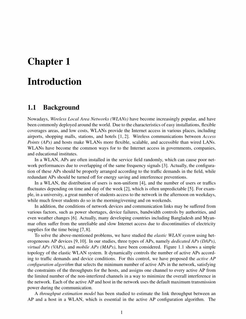
1.1 BackgroundNowadays, Wireless Local Area Networks (WLANs) have become increasingly popular, and havebeen commonly deployed around the world. Due to the characteristics of easy installations, flexiblecoverages areas, and low costs, WLANs provide the Internet access in various places, includingairports, shopping malls, stations, and hotels [1, 2]. Wireless communications between AccessPoints (APs) and hosts make WLANs more flexible, scalable, and accessible than wired LANs.WLANs have become the common ways for to the Internet access in governments, companies,and educational institutes.

In a WLAN, APs are often installed in the service field randomly, which can cause poor net-work performances due to overlapping of the same frequency signals [3]. Actually, the configura-tion of these APs should be properly arranged according to the traffic demands in the field, whileredundant APs should be turned off for energy saving and interference preventions.

In a WLAN, the distribution of users is non-uniform [4], and the number of users or trafficsfluctuates depending on time and day of the week [2], which is often unpredictable [5]. For exam-ple, in a university, a great number of students access to the network in the afternoon on weekdays,while much fewer students do so in the morning/evening and on weekends.

In addition, the conditions of network devices and communication links may be suffered fromvarious factors, such as power shortages, device failures, bandwidth controls by authorities, andeven weather changes [6]. Actually, many developing countries including Bangladesh and Myan-mar often suffer from the unreliable and slow Internet access due to discontinuities of electricitysupplies for the time being [7, 8].

To solve the above-mentioned problems, we have studied the elastic WLAN system using het-erogeneous AP devices [9, 10]. In our studies, three types of APs, namely dedicated APs (DAPs),virtual APs (VAPs), and mobile APs (MAPs), have been considered. Figure 1.1 shows a simpletopology of the elastic WLAN system. It dynamically controls the number of active APs accord-ing to traffic demands and device conditions. For this control, we have proposed the active APconfiguration algorithm that selects the minimum number of active APs in the network, satisfyingthe constraints of the throughputs for the hosts, and assigns one channel to every active AP fromthe limited number of the non-interfered channels in a way to minimize the overall interference inthe network. Each of the active AP and host in the network uses the default maximum transmissionpower during the communication.

A throughput estimation model has been studied to estimate the link throughput between anAP and a host in a WLAN, which is essential in the active AP configuration algorithm. The

1

parameter values of the model are optimized by throughput measurement results with different hostlocations in the network field. To improve the estimation accuracy of the model, the parameteroptimization tool [11, 12] has been proposed to find the accurate parameter values such that theaverage difference between the measured throughput and the estimated one becomes minimal.

!" #!"$!"

%&'(%&'( %&'(

)*+,*

%&'(%&'(

-.(/0./(

1(2/0./(

1(2/0./(

Figure 1.1: Overview of Elastic WLAN.

However, in the previous studies of the elastic WLAN system and the active AP configurationalgorithm, the following drawbacks need to be solved for reducing the power consumption andbetter performance of the current research:

• Hosts often repeat joining and leaving in the WLAN. Thus, the network configuration shouldbe adaptive with this dynamic host behavior. Unfortunately, the current active AP config-uration algorithm can only find the whole solution of all the active APs at the same time,with their associated hosts and assigned channels for a given state of the traffic demandsand the device conditions in the network. Even if only one host joins or leaves the network,the current algorithm generates the totally new configuration without considering the currentstate. If some hosts are currently communicating with the Internet, they cannot be stoppedto change the associated APs. Thus, the new configuration must avoid this discontinuity ofcommunicating services.

• In the current implementation of the elastic WLAN system, a Linux PC including RaspberryPi is used for a host and an AP. Therefore, to increase the security and performance of thesystem, it is important to keep updating the system and application software to the latestversion. The user authentication is also inevitable to enhance the security of the system.

• In the current algorithm, each of active APs is running with the maximum transmissionpower. Usually, a significant number of APs is deployed in a WLAN, which may causea large power consumption of the network and increase the interference to other APs. Insuch environment, reducing the transmission power of APs is important to reduce the powerconsumption and interference. Hence, the efficient transmission power management of theAP while maintaining the network performance is a challenging task.

2

• Finally, the extensive measurements for the accurate parameter tuning in the throughputestimation model cause high labor costs. The host must be moved to many locations, and themeasurements can be done manually. Thus, the number of measurement locations should beminimized.

1.2 ContributionsIn this thesis, we have carried out the following research contributions.

As the first contribution, we propose the extension of the active AP configuration algorithmto overcome the discontinuity problem in the current algorithm [13–15]. In this extension, thecurrently communicating APs and hosts are designated as communicating APs and communicatinghosts for convenience. Any communicating AP is not deactivated and any communicating hostdoes not change the associated AP by the algorithm. Through numerical experiments using theWIMNET simulator [16] in two network instances, the effectiveness of the proposed extension isdemonstrated.

Furthermore, the proposed algorithm extension is implemented on the elastic WLAN systemtestbed to verify the practicality in the real system. In this testbed implementation, RaspberryPi [17] is adopted for the AP and Linux PC is for the host. The performance of this elastic WLANsystem testbed is evaluated through experiments in four scenarios, where the measured throughputsby the proposal are always higher than those by the comparison methods.

As the second contribution, we implement the system software update function for APs andhosts and user authentication function in the elastic WLAN system, to enhance the system perfor-mance and security [18]. The system software update function periodically downloads the latestsystem software to the local repository servers, and installs it into them. Every AP and user hostin the system accesses to this server to update the software. Then, the user authentication functionis implemented to authenticate a newly joining host using the RADIUS server. These functions areevaluated with the elastic WLAN system testbed using Linux PCs for hosts and Raspberry Pi forAPs.

As the third contribution, we propose two approaches for the transmission power minimizationto reduce the power consumption in the elastic WLAN system. The first approach is the extensionof the active AP configuration algorithm to reduce the energy consumption at each of the activeAPs [19, 20]. In this extension, the previous active AP configuration finds the active APs, AP-host associations, and AP channel assignments, assuming the use of the maximum transmissionpower. Then, it minimizes the transmission power of each active AP such that it satisfies theminimum throughput constraint. The throughput estimation model has been used to evaluate thethroughput for each transmission power, where the model parameter values are obtained fromextensive measurements by applying the parameter optimization tool [11, 12].

The effectiveness of the proposal was validated through simulations with the WIMNET simula-tor and experiments using the testbed in several network scenarios. Unfortunately, the throughputmeasurement of different transmission powers require a lot of labor costs for accurate model pa-rameters that needs to be minimized.

In the second approach, we propose the PI feedback control for the transmission power min-imization [21, 22]. The benefit of this approach is to avoid extensive measurements. The initialpower is examined from the difference between the measured received signal strength (RSS) at theAP from the host and the estimated RSS necessary for the target throughput. Then, the power isdynamically minimized by using the PI feedback control [23], such that the measured throughput

3

by iperf [24], achieves the target one. The proposal was implemented in the elastic WLAN systemtestbed. The experiment results in different network topologies confirmed the effectiveness of theproposal.

Finally, as the fourth contribution, we propose two measurement location minimization meth-ods for selecting host locations that can keep the original accuracy of the throughput estimationmodel [25, 26]. To reduce the number of locations while keeping the model accuracy, we considerthe conditions to select the measurement locations. We confirm the effectiveness of our proposalthrough experiments for IEEE 802.11n WLAN, where the throughput estimation error is not de-graded after the location minimization and the number of original measurements is reduced by60% and 86% by first method and second method respectively.

The four contributions in the thesis are summarized as follows:

• the proposal of the dynamic extension of the active AP configuration algorithm to deal withthe dynamic host behavior in the elastic WLAN system.

• the implementation of the system software update and user authentication functions for sys-tem security of the elastic WLAN system.

• the proposal of AP transmission power minimization methods using the throughput estima-tion model and the PI feedback control.

• the proposal of measurement location minimization methods to reduce the labor cost andtime for the throughput estimation model.

1.3 Thesis OutlineThe remaining part of this thesis is organized as follows.

In Chapter 2, we review IEEE 802.11 wireless network technologies related to this thesis,including the IEEE 802.11n protocols, features of IEEE 802.11n protocols, and software tools inthe Linux operating system.

In Chapter 3, we review our previous related studies.In Chapter 4, we describe the proposal of the dynamic extension of the active AP configuration

algorithm, the implementation in the elastic WLAN system testbed, and the evaluation throughsimulations using the WIMNET simulator and experiments using the testbed.

In Chapter 5, we describe the implementation of the system software update and user authen-tication functions for system security of the elastic WLAN system.

In Chapter 6, we describe the proposal of the static AP transmission power minimization ap-proach using the throughput estimation model and the evaluation of the proposal through simula-tions and testbed experiments.

In Chapter 7, we describe the proposal of the dynamic AP transmission power minimizationapproach using the PI feedback control, the implementation in the elastic WLAN system testbed,and the evaluation in various network fields.

In Chapter 8, we describe the proposal of two measurement location minimization methods forthroughput estimation model.

Finally, in Chapter 9, we conclude this thesis with some future works.

4

Chapter 2

IEEE 802.11 Wireless Network Technologies

In this chapter, we briefly introduce wireless network technologies for backgrounds of this dis-sertation. First, we review IEEE 802.11 protocols. Then, we discuss the IEEE 802.11n protocol,especially, the key features of the protocol. After that, we introduce the three different types of APsassumed in the active AP configuration algorithm and discuss the characteristics and the speed dif-ference between them. Finally, we outline some Linux tools and commands for WLANs that areused for measurements, and the implementation of elastic WLAN system.

2.1 802.11 WLAN OverviewIEEE 802.11 standards determine physical (PHY) and media access control (MAC) layer specifi-cations for implementing high-speed wireless local area network (WLAN) technologies. WLANis an extension to a wired LAN that enables the user mobility by the wireless connectivity andsupports the flexibility in data communications [27]. It can reduce the cabling costs in the homeor office environments by transmitting and receiving data over the air using radio frequency (RF)technology.

2.1.1 Advantages of WLANWLAN offers several benefits over the traditional wired networks. Specific benefits are includedin the following [27]:

• User mobility:In a wired network, users need to use wired lines to stay connected to the network. On theother hand, WLAN allows user mobility within the coverage area of the network.

• Easy and rapid deployment:WLAN can exclude the requirement of network cables between hosts and connection hubsor APs. Thus, the installation of WLAN can be much easier and quicker than wired LAN.

• Cost:The initial installation cost can be higher than the wired LAN, but the life-cycle cost can besignificantly lower. In the environment requiring frequent movements or reconfigurations ofthe network, WLAN can provide the long-term cost profit.

5

• Increased flexibility:The network coverage area by WLAN can be easily expanded because the network mediumis already everywhere.

• Scalability:WLAN can be configured in a variety of topologies suitable to applications. WLAN can sup-port both peer-to-peer networks suitable for a small number of users and full infrastructurenetworks of thousands of users.

2.1.2 IEEE 802.11 WLAN ComponentsIEEE 802.11 WLAN consists of four primary components as shown in Figure 2.1 [27]:

Distributed

System

Access PointWireless Medium

Station

Station

Station

Figure 2.1: Components of IEEE 802.11 WLANs.

• Stations or hosts:WLAN transfers data between stations or hosts. A station in WLAN indicates an electronicdevice such as a desktop/laptop PC, a smartphone, or a tablet that has the capability ofaccessing the network over the wireless network interface card (NIC).

• Access points (APs):An AP acts as the main radio transceiver or a generic base station for WLAN that plays thesimilar role as a hub/switch in a wired Ethernet LAN. It also performs the bridging functionbetween the wireless and the wired networks with some other tasks.

• Wireless medium:The IEEE 802.11 standard uses the wireless medium to flow the information from one hostto another host in a network.

• Distribution system:When several APs are connected together to form a large coverage area, they must com-municate with each other to trace the movements of the hosts. The distribution system isthe logical component of WLAN which serves as the backbone connections among APs. Itis often called as the backbone network used to relay frames between APs. In most cases,Ethernet is commonly used as the backbone network technology.

6

2.1.3 Operating Modes for IEEE 802.11 WLANThe elementary unit of IEEE 802.11WLAN is simply a set of hosts that can communicate witheach other known as the basic service set (BSS). Based on the types of BSS, the IEEE 802.11supports two operating modes as illustrated in Figure 2.2.

• Independent or ad hoc mode:In this mode, a collection of stations or hosts can send frames directly to each other withoutan AP. It is also called as an independent BSS (IBSS) mode as shown in Figure 2.2(a). This adhoc network is rarely used for permanent networks due to the lack of required performancesand security issues.

• Infrastructure mode:In this mode, the stations exchange their information through an AP as shown in Fig-ure 2.2(b). A single AP acts as the main controller to all the hosts within its BSS, knownas infrastructure BSS. In this mode, a host must be associated with an AP to obtain networkservices [28].

Station

StationStation

(a) Adhoc network.

Station

StationStation

Access

Point

(b) Infrastructure network.

Figure 2.2: Operating modes of IEEE 802.11 networks.

In addition, multiple BSSes can be connected together with a backbone network to formextended service set (ESS) as shown in Figure 2.3. ESS can form a large size WLAN. EachAP in ESS is given an ID called the service set identifier (SSID), which serves as a “networkname” for the users. Hosts within the same ESS can communicate with each other, even ifthey are in different basic service areas.

2.1.4 Overview of IEEE 802.11 ProtocolsThe IEEE 802.11 working group has improved the existing PHY and MAC layer specificationsto realize WLAN at the 2.4-2.5 GHz, 3.6 GHz and 5.725-5.825 GHz unlicensed ISM (Industrial,Scientific and Medical) frequency bands defined by the ITU-R. In this working group, severaltypes of IEEE Standard Association Standards are available, where each of them comes with aletter suffix, covers from wireless standards, to standards for security aspects, Quality of Service(QoS) and others, shown in Table 2.1 [28–33].

7

AP1AP2

Distributed System

StationStation

StationBSS1 BSS2

Figure 2.3: Extended service set (ESS).

Table 2.1: IEEE 802.11 Standards.

Standard Purpose

802.11a Wireless network bearer operating in the 5 GHz ISM band, data rate upto 54Mbps

802.11b Operate in the 2.4 GHz ISM band, data rates up to 11Mbps802.11c Covers bridge operation that links to LANs with a similar or identical

MAC protocol802.11d Support for additional regulatory differences in various countries802.11e QoS and prioritization, an enhancement to the 802.11a and 802.11b

WLAN specifications802.11f Inter-Access Point Protocol for handover, this standard was withdrawn802.11g Operate in 2.4 GHz ISM band, data rates up to 54Mbps802.11h Dynamic Frequency Selection (DFS) and Transmit Power Control

(TPC)802.11i Authentication and encryption802.11j Standard of WLAN operation in the 4.9 to 5 GHz band to conform to

the Japan’s rules802.11k Measurement reporting and management of the air interface between

several APs802.11l Reserved standard, to avoid confusion802.11m Provides a unified view of the 802.11 base standard through continuous

monitoring, management and maintenance802.11n Operate in the 2.4 and 5 GHz ISM bands, data rates up to 600Mbps802.11o Reserved standard, to avoid confusion802.11p To provide for wireless access in vehicular environments (WAVE)802.11r Fast BSS Transition, supports VoWiFi handoff between access points to

enable VoIP roaming on a WiFi network with 802.1X authentication802.11s Wireless mesh networking802.11t Wireless Performance Prediction (WPP), this standard was cancelled

8

Table 2.1: IEEE 802.11 Standards.

Standard Purpose

802.11u Improvements related to ”hotspots” and 3rd party authorization ofclients

802.11v To enable configuring clients while they are connected to the network802.11w Protected Management Frames802.11x Reserved standard, to avoid confusion802.11y Introduction of the new frequency band, 3.65-3.7GHz in US besides 2.4

and 5 GHz802.11z Extensions for Direct Link Setup (DLS)802.11aa Specifies enhancements to the IEEE 802.11 MAC for robust audio video

(AV) streaming802.11ac Wireless network bearer operating below 6 GHz to provide data rates of

at least 1Gbps for multi-station operation and 500Mbps on a single link802.11ad Wireless Gigabit Alliance (WiGig), providing very high throughput at

frequencies up to 60GHz802.11ae Prioritization of management frames802.11af WiFi in TV spectrum white spaces (often called White-Fi)802.11ah WiFi uses unlicensed spectrum below 1GHz, smart metering802.11ai Fast initial link setup (FILS)802.11aj Operation in the Chinese Milli-Meter Wave (CMMW) frequency bands802.11ak General links802.11aq Pre-association discovery802.11ax High efficiency WLAN, providing 4x the throughput of 802.11ac802.11ay Enhancements for Ultra High Throughput in and around the 60GHz

Band802.11az Next generation positioning802.11mc Maintenance of the IEEE 802.11m standard

Figure 2.4 shows the current and future WiFi standards. Among these standards, the commonand popular ones are IEEE 802.11a, 11b, 11g, 11n, and 11ac. For the physical layer, the 11a/n/acuse Orthogonal Frequency Division Multiplexing (OFDM) modulation scheme while the 11b usesthe Direct Sequence Spread Spectrum (DSSS) technology. 11g supports both technologies. Ta-ble 2.2 summarizes the features of these common WiFi standards [27, 34, 35].

• IEEE 802.11b: IEEE 802.11b operates at 2.4 GHz band with the maximum data rate up to11 Mbps. 11b is considered to be a robust system and has a capacity to compensate thesame IEEE 802.11 protocols. Because of the interoperability feature between products fromdifferent vendors, this standard has not only boosted the manufacturing of the products butalso motivated the competitions between WLAN vendors. The limitation of this standard isthe interference among the products using industrial, scientific and medical (ISM) band thatuses the same 2.4 GHz band of frequency [36, 37].

• IEEE 802.11a: IEEE 802.11a operates at 5 GHz ISM band. It adopts on orthogonal fre-quency division multiplexing (OFDM) coding scheme that offers a high data rates up to 6,

9

Figure 2.4: Current and future WiFi Standards.

Table 2.2: Characteristics of common IEEE 802.11 standards.

IEEE IEEE IEEE IEEE IEEE802.11b 802.11a 802.11g 802.11n 802.11ac

Release Sep 1999Sep1999

Jun 2003 Oct 2009 Dec 2013

Frequency Band 2.4 GHz 5 GHz 2.4 GHz2.4/5GHz

5 GHz

Max. Data Rate 11 Mbps 54 Mbps 54 Mbps600

Mbps1300 Mbps

ModulationCCK1modulated with

PSKOFDM

DSSS2,CCK,

OFDMOFDM OFDM

Channel Width 20 MHz 20 MHz 20 MHz20/40MHz

20/40/80/160MHz

# of Antennas 1 1 1 4 8security Medium Medium Medium High High

1 CCK: Complementary Code Keying2 DSSS: Direct Sequence Spread Spectrum

12, 24, 54 Mbps, and sometimes beyond this speed in comparison to 11b. Two main lim-itations of 11a are the compatibility issue of the 11a products with 11b products and theunavailability of 5 GHz band with free of cost for all the countries in the world [36, 37].

• IEEE 802.11g: IEEE suggested 11g standard over 11a to improve the 2.4 GHz 11b tech-nology. 11g introduces two different modulation techniques including the packet binaryconvolution code (PBCC) that supports the data rate up to 33Mbps and the orthogonal fre-quency division multiplexing (OFDM) that supports up to 54Mbps data rate. Compatibilityissues are also resolved in 11g products with 11b products [36, 37].

• IEEE 802.11n: The primary purpose of initiating the 11n standard to improve the usablerange and data rate up to 600Mbps. 11n supports both of 2.4 GHz and 5 GHz ISM bandunlicensed national information infrastructure (UNII) band, and is backward compatiblewith earlier standards. It introduces new technology features including the use of channelbonding and multiple antennas to get the better reception of the RF signals to enhance thethroughput and coverage range [36, 38].

10

• IEEE 802.11ac: The aim of the 11ac standard to improve individual link performance andtotal network throughput of more than 1Gbps. Many of the specifications like static and dy-namic channel bonding and simultaneous data streams of 11n have been kept and further en-hanced for 11ac to reach the gigabit transmission rate. It supports static and dynamic channelbonding up to 160MHz and Multi-User Multiple-Input-Multiple-Output (MU-MIMO). 11acoperates only on the 5 GHz band [39–41].

2.2 IEEE 802.11n ProtocolIn this section, we overview the IEEE 802.11n protocol that has been used for our throughputmeasurements and implementations. IEEE 802.11n is an amendment to the IEEE 802.11 2007wireless networking standard. This standard was introduced with 40 MHz bandwidth channels,Multiple-Input-Multiple-Output (MIMO), frame aggregation, and security improvements over theprevious 11a, 11b, and 11g standards. Table 2.3 shows a brief summary of this standard.

Table 2.3: IEEE 802.11n specification.

Specification IEEE 802.11nFrequency Band 2.4 GHz 5 GHzSimultaneous Uninterrupted Channel 2 ch 9 chAvailable Channel 13 ch 19 chMax. Speed 600MbpsMax. Bandwidth 40 MHzMax. Spatial Streams 4Subcarrier Modulation Scheme 64 QAMRelease Date Sept 2009

The IEEE 802.11n is available both on 2.4 GHz and 5 GHz bands. Nowadays, 2.4 GHz is verypopular as it was inherited from the IEEE 802.11g. This frequency band has become crowdedwith lots of WiFi signals using the same channel. As a result, these WiFi signals with adjacentchannels will suffer from interferences between them, and end up with throughput performancedegrades [32, 34]. For 2.4 GHz band, there is a limited number of non-interfered channels, whichare Channel 3 and Channel 11 in 40 MHz bandwidth. While for 20 MHz bandwidth, Channel 1,Channel 6, and Channel 11 are free from interference. In overall, the wider bandwidth will reducethe number of free channels. Figure 2.5 [33] shows the WiFi channels for IEEE 802.11n 2.4 GHzband. In the 5 GHz band of IEEE 802.11n protocol, it has 19 uninterrupted channels availablewith the 20MHz bandwidth. In the 40MHz bandwidth, which doubles the channel width from the20MHz, there are nine channels. For the 80MHz bandwidth, there are four of them. Figure 2.6shows these WiFi channels for the IEEE 802.11n 5 GHz band [42].

2.3 Features of IEEE 802.11n ProtocolIEEE 802.11n protocol incorporates several new technologies to boost up its performance. Thestandard uses the multiple antennas technology, channel bonding, frame aggregation, and security

11

1ch 2ch 3ch 4ch 5ch 6ch 7ch 8ch 9ch 10ch 11ch12ch13ch

20MHz

2412MHz 2432MHz 2452MHz 2472MHz

5MHz

Figure 2.5: WiFi channels in 2.4 GHz band.

Figure 2.6: WiFi channels in 5 GHz band.

improvements mechanism to improve the throughput. In this section, we describe these featuresof IEEE 802.11n Protocol.

• Channel Bonding:In the channel bonding, each channel can operate with the 40MHz bandwidth by using twoadjacent 20MHz channels together to double its physical data rate [43] as shown in Fig-ure 2.7. However, the usage of the channel bonding will reduce the available non-interferedchannels for other devices as there are only two non-interfered bonded channels availablefor IEEE 802.11n protocol at 2.4 GHz band. Table 2.4 shows the usage of different channelbandwidths and spatial streams towards the throughput of IEEE 802.11n.

• MIMO (Multiple-Input-Multiple-Output):In MIMO, the throughput can be linearly increased to the number of transmitting (TX) andreceiving (RX) antennas up to four times, without the additional bandwidth or transmissionpower. The coverage area can be enhanced over the single antenna technology in Single-Input Single-Output (SISO). The multiple antenna configurations in MIMO can overcome thedetrimental effects of multi-path and fading, trying to achieve high data throughput in limitedbandwidth channels. For example, in the 4× 4 MIMO, four independent data streams can bemultiplexed and transmitted simultaneously with the spatial division multiplexing (SDM), to

12

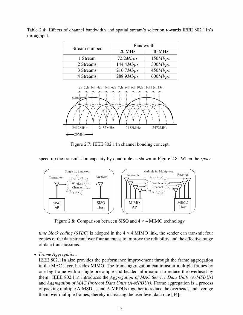
Table 2.4: Effects of channel bandwidth and spatial stream’s selection towards IEEE 802.11n’sthroughput.

Stream number Bandwidth20 MHz 40 MHz

1 Stream 72.2Mbps 150Mbps2 Streams 144.4Mbps 300Mbps3 Streams 216.7Mbps 450Mbps4 Streams 288.9Mbps 600Mbps

1ch 2ch 3ch 4ch 5ch 6ch 7ch 8ch 9ch 10ch 11ch12ch13ch

20MHz

2412MHz 2432MHz 2452MHz 2472MHz

5MHz

Figure 2.7: IEEE 802.11n channel bonding concept.

speed up the transmission capacity by quadruple as shown in Figure 2.8. When the space-

Transmitter ReceiverMultiple in, Multiple out

SISO

AP

Transmitter Receiver

Wireless

Channel

Single in, Single out

MIMO

AP

MIMO

Host

Wireless

Channel

SISO

Host

Figure 2.8: Comparison between SISO and 4 × 4 MIMO technology.

time block coding (STBC) is adopted in the 4 × 4 MIMO link, the sender can transmit fourcopies of the data stream over four antennas to improve the reliability and the effective rangeof data transmissions.

• Frame Aggregation:IEEE 802.11n also provides the performance improvement through the frame aggregationin the MAC layer, besides MIMO. The frame aggregation can transmit multiple frames byone big frame with a single pre-ample and header information to reduce the overhead bythem. IEEE 802.11n introduces the Aggregation of MAC Service Data Units (A-MSDUs)and Aggregation of MAC Protocol Data Units (A-MPDUs). Frame aggregation is a processof packing multiple A-MSDUs and A-MPDUs together to reduce the overheads and averagethem over multiple frames, thereby increasing the user level data rate [44].

13

• Modulation and Coding Scheme:Various modulation, error-correcting codes are used in IEEE 802.11n, represented by a Mod-ulation and Coding Scheme (MCS) index value, or mode. IEEE 802.11n defines 31 differentmodes and provides the greater immunity against selective fading by using the OrthogonalFrequency Division Multiplexing (OFDM). This standard increases the number of OFDMsub-carriers of 56 (52 usable) in High Throughput (HT) with 20MHz channel width and114 (108 usable) in HT with 40MHz. Each of these sub-carriers is modulated with BPSK,QPSK, 16-QAM or 64-QAM, and Forward Error Correction (FEC) coding rate of 1/2, 2/3,3/4 or 5/6 [44].

2.4 Heterogeneous Access PointsIn this section, we introduce three different types of APs that we use in our active AP configurationalgorithm. We also discuss the characteristics and the speed difference of these APs.

A DAP is a wireless AP that adopts the IEEE 802.11n wireless protocol and connects PCs tothe Internet. A commercial DAP using IEEE 802.11n has the coverage radius of around 110m andthe transmission speed around 120Mbps. However, the transmission speed varies significantlydepending on the environment including obstacles, channel interferences, number of antennas andplacement heights of APs.

A VAP is a software-based router using a personal computer (PC) with either Windows orLinux for the operating system. Several Internet connection mediums including wired, wireless,or cellular communications are available for the VAP. A network device can connect to a VAP thesame way as it does to a conventional DAP. Most VAPs support the IEEE 802.11n protocol [45]with a maximum of 54Mbps transmissions.

While, DAP and VAP use wired Ethernet to access the Internet, the MAP is a device that con-nects to the Internet through 3G/4G wireless technology, e.g., smart phone. For such portabledevices, the power supply is unnecessary because of the built-in battery. With the rapid devel-opment of the cellular technology, most MAPs support the IEEE 802.11n protocol, in which thetransmission speed is capped to around 30Mbps due to the bottleneck in the cellular network1.

2.5 Linux Tools for Wireless NetworkingAs an open-source operating system, Linux has been used as a platform to implement new al-gorithms, protocols, methods, and devices for advancements of wireless networks [46]. In thissection, we give the overview of the Linux tools and software used for the measurement performedthroughout the thesis and the implementation of the elastic WLAN system.

2.5.1 ‘arp-scan’ - to Explore Currently Active Devicesarp-scan [47] is a command-line tool using the ARP protocol to discover and fingerprint the IPhosts in the local area network. This tool can discover all the devices using IP addresses in thenetwork. arp-scan works on an IEEE 802.11 wireless (WiFi) network as well as a wired Ethernet,

1We should note that the DAPs and the VAPs share the gateway to the Internet. The bandwidth of this gatewaybecomes the total available bandwidth for the whole WLAN.

14

where the wireless network uses the same data-link protocol. In the Linux operating system, arp-scan can be installed by downloading the source code from [48] or using the following command:

$ sudo ap t −g e t i n s t a l l arp −s can

The simplest command to scan the network using arp-scan is given by:

$ arp −s can −− i n t e r f a c e =e t h 0 −− l o c a l n e t

–interface=eth0 represents the interface to be used in scanning devices. The use of –localnet makesarp-scan scan all the possible IP addresses in the network that are connected to this interface, whichis defined by the interface IP address and net mask. The name of the network interface depends onthe operating system, the network type (Ethernet, wireless etc.), and the interface card type. Here,the interface name eth0 is used as an example.

2.5.2 ‘nm-tool’ - to Collect Host Informationnm-tool provides the information of the devices in the local area network including the wirelessnetwork [49, 50]. In our design, we use nm-tool to get the information for the host such as thecurrently associated AP, the associable APs, and the receiving signal strength from each AP. nm-tool is installed as a part of the NetworkManager package [51] in the Linux operating system,which is usually installed by default on the Ubuntu distribution. It can be installed using thefollowing command manually:

$ sudo ap t −g e t i n s t a l l network−manager

The simple way to run nm-tool is:

$ nm− t o o l

2.5.3 ‘hostapd’ - to Make AP-mode Linux-PChostapd is a Linux tool for the AP and the authentication server. It implements IEEE 802.11 APmanagements, along with other IEEE 802.1X protocols and security applications. In the Linuxoperating system, hostapd can be installed by downloading the source code from [52] or using thefollowing command:

$ sudo ap t −g e t i n s t a l l h o s t a p d

After installing this tool in a Linux PC that contains WLAN driver that supports the AP mode, itcan be configured to create a command-line based AP in the Linux-PC. The hostapd can be startedor stopped by the following commands:

$ sudo / e t c / i n i t . d / h o s t a p d s t a r t$ sudo / e t c / i n i t . d / h o s t a p d s t o p

2.5.4 ‘ssh’ - to Remotely Execute Commandssh is an abbreviation of Secure Shell that is a cryptographic network protocol to securely initiate ashell session on a remote machine [53, 54]. It is operated in two parts: SSH client and SSH server,and establishes a secure channel between them over an insecure network. The open source versionof ssh is OpenSSH [55] that can be installed using the following command [56]:

15

$ sudo ap t −g e t i n s t a l l openssh − s e r v e r openssh − c l i e n t

The following list shows an example to remotely execute nm-tool on a remote host through thenetwork using ssh [53, 54, 57]:

$ s s h username@192 . 1 6 8 . 1 . 3 1 ’nm− t o o l ’username@192 . 1 6 8 . 1 . 3 1 ’ s password :

Here, 192.168.1.31 represents the IP address of the remote host.

2.5.5 ‘nmcli’ - to Change Associated APnmcli [58, 59] is a command-line Linux tool to manage, configure, and control the powerful Net-workManager package. nmcli is pre-included in the NetworkManager package. nmcli is used toassociate a host with an AP through the following command line:

$ sudo −s nmcl i dev w i f i c o n n e c t NewSSID password PASSWORD

The above command connects the host to the AP specified with NewSSID using the correspondingpassword PASSWORD of the AP.

2.5.6 ‘iwconfig’ - to Collect Information of Active Network Interfaceiwconfig [60] is a command-line Linux tool to display and change the parameters of the activenetwork interface for wireless operations. It can also be used to display the wireless networkparameters and statistics. iwconfig is usually installed by default in the Ubuntu distribution. It canalso be installed manually using the following command:

$ sudo ap t −g e t i n s t a l l w i r e l e s s − t o o l s

The following list shows the use of iwconfig to display the information of the currently associatedAP using the network interface wlan0:

$ i w c o n f i g wlan0

2.5.7 ‘iperf’ - to Measure Link Speediperf [24] is a software to measure the available throughput or bandwidth on IP networks. Itsupports both TCP and UDP protocols along with tuning various parameters related to timing andbuffers, and reports the bandwidth, the loss, and other parameters. iperf is usually installed bydefault in the Ubuntu distribution. It can also be installed manually using the following command:

$ sudo ap t −g e t i n s t a l l i p e r f

To measure the TCP throughput between two devices using iperf, one of them uses the server-mode and the other one uses the client-mode, where packets are transmitted from the client to theserver. The iperf output contains the time-stamped report of the transmitted data amount and themeasured throughput. The following list shows the typical use of iperf on the server and client sidefor throughput measurement:

$ i p e r f −s / / s e r v e r s i d e$ i p e r f −c 1 7 2 . 2 4 . 4 . 1 / / c l i e n t s i d e

Here, 172.24.4.1 represents the IP address of the server. In this thesis, we use iperf to measure thethroughput between an AP and a host through the IEEE802.11n protocol.

16

2.6 SummaryIn this chapter, we presented various wireless network technologies, key features of IEEE 802.11nprotocols, heterogeneous WLAN AP devices and Linux tools which are adopted in this thesis forour experiments as well as simulations. In the next chapter, we will review our previous relatedstudies.

17

Chapter 3

Review of Previous Studies

In this chapter, we briefly overview our previous studies related to this thesis. Firstly, we reviewthe elastic WLAN system. Secondly, we review the study of the throughput estimation model forthe IEEE 802.11n link in WLAN. Thirdly, we review the study of the active AP configurationalgorithm for the elastic WLAN system. Finally, we review the implementation details of theelastic WLAN system testbed using Raspberry Pi APs.

3.1 Elastic WLAN SystemIn this section, we review the elastic WLAN system, which can dynamically optimize the networkconfiguration by activating/deactivating APs, according to traffic demands and network conditions.

3.1.1 OverviewCurrently, WLANs have been increasingly installed in business organizations, educational institu-tions, and public places like buses, airplanes, or trains. In these cases, unplanned or independentlycontrolled APs can lead to problems resulting in performance degradations and/or wastages of en-ergy. In one hand, WLANs can suffer from over-allocation problems with redundant APs that haveoverlapped coverage areas. On another hand, WLANs can be overloaded with hosts suffering fromlow performances. Therefore, WLANs should be adaptive by changing the allocations of APs andthe associations of hosts to the APs, according to the network traffic demands and conditions. Torealize this goal, we have studied the elastic WLAN system.

3.1.2 Related Works in LiteratureIn this section, we show our brief surveys to this work.

In [61], Lei et al. proposed a campus WLAN framework based on the software defined network(SDN) technology.

In [62], Luengo et al. also proposed a design and implementation of a testbed for integratedwireless networks based on SDN. Although this framework is flexible to design and manage, itrequires SDN-enabled devices and network virtualizations.

In [63][64], Sukaridhoto et al. proposed a Linux implementation design using OpenFlow of thefixed backoff-time switching (FBS) method for the wireless mesh network. Their implementationrequires Linux driver kernel modifications and specific WLAN hardware interfaces.

19

In [65], Ahmed et al. describe the important design issues in preparing a large-scale WLANtestbed for evaluation of centralized control algorithms and presented experimental results. Theydid not analyzed the power-saving and adaptive control mechanism of centralized WLANs whichis one of the the main purposes of our research.

In [66], Debele et al. proposed a Resource-on-Demand (RoD) strategy for energy-saving indense WLANs where they analyzed user behavior in the network and formulated the stochasticcharacteristics. Our system also adapts with the user demand and frequency, and moreover wepresent a implementation of our system in real networks.

3.1.3 Design and Operational FlowFigure 3.1 illustrates an example topology of the elastic WLAN system. The elastic WLAN systemdynamically controls the number of active APs in the network by activating or deactivating theinstalled APs according to traffic demands and network conditions. The implementation of the

!"#$%

&'(')$*$(#

+$%,$%

-.%$/0

1!(($2#.!(

-.%$3$440

1!(($2#.!(

522$4406!.(#522$4406!.(#

7!4# 7!4# 7!4# 7!4#

Figure 3.1: Design of Elastic WLAN system.

elastic WLAN system adopts the management server to manage the necessary information for thesystem and control the APs and the hosts. This server not only has the administrative access rightsto all the devices in the network, but controls the whole system through the following three steps:

1. The server explores all the devices in the network and collects the requisite information forthe active AP configuration algorithm.

2. The server executes the active AP configuration algorithm using the inputs derived in theprevious step. The output of the algorithm contains the list of the active APs, the hostassociations, and the assigned channels.

3. The server applies this output to the network by activating or deactivating the specified APs,changing the specified host associations, and assigning the channels.

20

3.2 Throughput Estimation Model for IEEE 802.11n ProtocolThe link speed or throughput between any AP and host depends on a variety of factors such as themodulation and coding scheme, the transmission power, the transmission distance, and obstacles.The theoretical computation of the accurate link speed is challenging [9][67]. In this section, wereview the throughput estimation model for IEEE 802.11n link in WLAN.

3.2.1 Overview of ModelThis model estimates the link speed or data throughput of an IEEE 802.11 link in WLAN. It hastwo main steps to estimate the throughput between a source and a destination node. In the firststep, it estimates the receiving signal strength (RSS) at the host by using the log distance path lossmodel. In the second step, it converts the estimated RSS into the corresponding throughput by thesigmoid function [11]. Both functions have several configuration parameters that can affect theestimation accuracy, which depends on link specifications and network field environments.

3.2.2 Receiving Signal Strength Estimation by Log-Distance Path ModelThe signal strength is estimated by the log-distance path loss model and it considers the multi-patheffects by considering both the direct signal along the line-of-sight (LoS) and the indirect signalthrough the non line-of-sight (NLoS) path in indoor environments. First, the Euclidean distance d(m) is calculated for each link (AP/host pair) by:

d =

√(APx − Hx)2 + (APy − Hy)2 (3.1)

where APx, APy and Hx, Hy does the x and y coordinates for the AP and the host respectively. Then,the RSS, Pd (dBm), at the host is estimated using the log distance path loss model by consideringthe distance and the obstacles loss between end nodes[67]:

Pd = P1 − 10α log10 d −∑

k

nkWk (3.2)

where P1 represents the signal strength at 1m from the AP (source), α is the path loss exponent,d (m) does the link distance from the AP, nk does the number of the type-k walls along the pathbetween the AP and the host, and Wk does the signal attenuation factor (dBm) for the type-k wallin the environment. The estimation accuracy of RSS relies on the parameter values, which dependon the propagation environment [67].

3.2.3 Throughput Estimation by Sigmoid FunctionFrom the RSS, the throughput S (Mbps) of the link is derived using following the sigmoid function:

S =a

1 + e−( (Pd+120)−bc )

(3.3)

where a, b, and c are the constant parameters of the sigmoid function that should be optimizedby parameter optimization tool [12]. The assumption of this sigmoid function for the throughputestimation is based on our real-world measurement results which clearly reflects the relationshipbetween the RSSs and the estimated throughput.

21

3.2.3.1 Multi-Path Effect Consideration

Due to the multipath effect in indoor environments, the receiver may receive the indirect signalthrough an NLoS path that arrives after reflected/diffracted at some points on walls or obstacles,in addition of the direct signal along the LOS path. When the direct signal passes through multi-ple walls, the RSS at the receiver becomes much weaker than that of the indirect signal if it passesthrough much fewer walls. The throughput estimation model considers this multi-path effect by se-lecting a diffraction point for each AP/host pair such that it is located on the wall in the same roomas the host and RSS of the AP is largest. The indirect signal reaches the host through this diffractingpoint after the signal is attenuated there. The RSS through indirect path, Pind is calculated by:

Pdi f = P1 − 10α log10 r −∑

k

nkWk (3.4)

Pind = Pdi f − 10α log10 t −Wdi f (3.5)

where Pdi f represents the RSS at the diffraction point, r (m) is the distance between the AP and thediffraction point, t (m) does the distance between the diffraction point and the host, and Wdi f (dBm)does the attenuation factor at the diffraction point. For the estimated RSS at the receiver, the largerone between the direct or indirect signals is selected.

3.3 Active AP Configuration AlgorithmIn this section, we review the active AP configuration algorithm for the elastic WLAN system thatoptimizes the number of active APs and the host associations [9, 10].

3.3.1 Problem FormulationThe active AP configuration problem for this algorithm is formulated as follows:

1. Inputs:

• Number of hosts: H

• Number of APs: N = ND + NV + NM where ND, NV , and NM represent the number ofDAPs, VAPs, and MAPs respectively.

• Link speed between APi and host j for i = 1 to N, j = 1 to H: si j, where the linkspeed can be estimated by the model in [11].

• Minimum link speed for association: S

• Number of non-interfered channels: C

2. Outputs:

• Set of active APs

• Set of hosts associated with each active AP

• Channel assigned to each active AP

3. Objectives:

22

• To minimize E1.

• Holding the first objective, to maximize E2.

• Holding the two objectives, to minimize E3 for channel assignments.

Let, E1 represents the number of active APs (DAPs, VAPs, and MAPs) in the network:

E1 = ED1 + EV

1 + EM1 (3.6)

where ED1 represents the number of active DAPs, EV

1 does the number of active VAPs, andEM

1 does the number of active MAPs respectively.The transmission delay of the jth AP can be defined by:

T j =∑k∈P j

Dk

s jk(3.7)

where Dk represents the traffic of the kth host, s jk does the link speed between the jth AP tothe kth host, and P j does the set of the hosts associated with the jth AP. Then, the averagethroughput T Hi j of the ith host associated with the jth AP can be estimated by:

T Hi j =Di

T j=

Di∑k∈P j

Dks jk

(3.8)

Since the real traffic of each host is unpredictable, we assume the identical traffic for everyhost, which can be represented by the unit traffic for the sake of simplicity. Then, the averagehost throughput for AP j is given by:

T H j =1∑

k∈P j

1s jk

(3.9)

If T H j ≥ G, the minimum host throughput constraint is satisfied, where G represents thethreshold for this constraint. Then, the second objective function E2 is defined to maximizethe minimum average host throughput for the bottleneck, AP which is given by:

E2 = minj

[T H j

](3.10)

E3 signifies the total interfered communication time:

E3 =

N∑i=1

[ITi] =

N∑i=1

∑k∈Iick=ci

Tk

(3.11)

where ITi represents the interfered communication time for APi, Ti does the total communi-cation time for APi, Ii does the set of the interfered APs with APi, and ci does the assignedchannel to APi. They are given by follows:

• Tk is given by the sum of the time that is required to transmit one bit data between APk

and its each associated host.

23

• Ii represents the set of the indices of the APs that are interfered with APi if they areassigned the same channel.

• ck signifies the channel assigned to APk by the active AP configuration algorithm.

• ITi is given by the sum of the total communication time for the APs that are interferedwith APi.

4. Constraints:

• Minimum host throughput constraint: each host in the network must enjoy the giventhreshold G on average when all the hosts are communicating simultaneously.

• Bandwidth limit constraint: the bandwidth of the wired network to the Internet must beless than or equal to the total available bandwidth of the network Ba.

• Channel assignment constraint: each AP must be assigned one channel between 1 andC.

3.3.2 Algorithm ProcedureThe active AP configuration algorithm consists of three phases: the active AP and associated hostselection phase, the channel assignment phase, and the channel load averaging phase.

3.3.2.1 Active AP and Associated Host Selection Phase

In this phase, the set of the active APs and their associated hosts are selected. This phase comprisesfollowing eight steps:

1. PreprocessingThe link speed for each possible pair of an AP and a host is estimated with the measurementor the throughput estimation model [11]. Then, this step initializes the variables for thefollowing steps:

(a) For each AP, make a list of hosts that can be associated with this AP, where the through-put of the link between a host and an AP is S or larger, it can be associated. This list iscalled the associable host list for APs.

(b) Initialize each AP as the non-active AP. Initially, only the DAPs are selected as candi-date APs.

2. Initial Solution GenerationAn initial solution to the cost function E1 is derived using a greedy algorithm [68], whichrepeats the following procedures:

(a) Select the AP that can be associated with the maximum number of non-associatedhosts.

(b) Activate this AP and increment E1 by one.

(c) Update the number of non-associated hosts in the host list for APs.

3. Host Association ImprovementThe cost function E2 is calculated for the greedy solution using Eq. (3.10). Then, this

solution is improved by repeating the following procedure:

24

(a) Find the AP that gives the lowest host throughput in Eq. (3.10).

(b) Select one host randomly from the associated hosts with this AP, and associate it withanother active AP that is selected randomly. Then, calculate E2.

(c) Keep the new association only if this new E2 is higher than the previous E2. Otherwise,return to the previous association.

4. AP Selection OptimizationThe cost functions E1 and E2 are further jointly improved in this step under the constraints

mentioned before by the local search [69]. This local search repeats the following threeprocedures:

(a) If the current solution satisfies the minimum host throughput constraint, it seeks to re-duce the number of active APs E1 by deactivating an active AP. In the implementation,it repeats to 1) randomly select an active AP and deactivate it, 2) apply Host AssociationImprovement, and 3) check the feasibility of this deactivation.

(b) Otherwise, it seeks to improve the minimum average host throughput E2 with the samenumber of active APs by changing the active AP. In the implementation, it repeats to1) randomly select a non-active AP and activate it, 2) apply Host Association Improve-ment, and 3) check the possibility of deactivating another active AP.

(c) If (b). is not achieved, it seeks to satisfy the minimum host throughput constraint by in-creasing the number of active APs while improving the minimum average host through-put. In the implementation, it 1) randomly selects a non-active AP and 2) applies HostAssociation Improvement.

5. Link Speed NormalizationThe fairness criterion will be applied when the total expected bandwidth exceeds Ba. Gen-erally, the link speed is normalized as:

(a) Calculate the expected total bandwidth Be by the summation of the throughputs of allthe APs.

(b) If Be>Ba, adjust each AP-host link speed as:

si j = si j ×Ba

Be (3.12)

where si j is the normalized link speed.

6. Termination CheckThe algorithm is terminated when either of the following conditions is satisfied:

(a) The minimum host throughput constraint is satisfied.

(b) All the APs in the network have been activated.

7. Additional VAP ActivationIf all the DAPs become active but the minimum host throughput constraint is still not sat-isfied, VAPs are newly selected as candidate APs. A VAP is slower than a DAP, but fasterthan a MAP. The locations of hosts are considered as the locations of the candidate VAPs,because user hosts may be used for VAPs. Then, it returns to AP Selection Optimizationstep.

25

8. Additional MAP ActivationIf all the DAPs and VAPs become active but the minimum host throughput constraint is stillnot satisfied, MAPs are newly selected as candidate APs. A MAP is the slowest amongthe three AP types. The locations of hosts are considered as the locations of the candidateMAPs, because users may have MAPs. Then, it returns to AP Selection Optimization step.

3.3.2.2 Channel Assignment Phase

In this phase, the assigned channels to the active APs are selected and it has the following foursteps:

1. PreprocessingThe interference and delay conditions of the network are represented by a graph.

(a) Construct the interference graph, G = (V, E), from the APs and the hosts, where thevertex V represents the set of APs and the edge E presents the existence of the interfer-ence between two APs. e(i, j) ∈ E if APi is interfered with AP j in the network.

(b) Calculate the communication time for each AP. The communication time Ti for APi isdefined as the total time when the AP transmits 1-bit to all the associated hosts. It isgiven by:

Ti =∑

j

1spi j

(3.13)

where spi j represents the link speed between APi and host j.

(c) Calculate the neighbor interfered communication time for each AP. The neighbor in-terfered communication time NTi for APi is given by:

NTi =∑

e(i,k)=1

Tk (3.14)

2. Interfered AP Set GenerationThe set of APs that are interfering with each other is found for each AP.

(a) Sort the APs in descending order of NTi, where the tie-break is resolved by Ti.

(b) Find the interfered AP set for each AP by repeating the following steps:

i. Initialize the interfered AP set by Ii = {i} for APi.ii. Expand Ii by examining the APs in sorted order in a) whether the AP is interfered

with each AP in Ii. If so, include this AP, AP j, into Ii, i.e. Ii = Ii ∪ { j}.

(c) Calculate the total interfered communication time ATi for APi, which is given by:

ATi =∑k∈Ii

Tk (3.15)

3. Initial Solution ConstructionThen, an initial solution is derived with a greedy algorithm.

(a) Sort the APs in descending order of the total interfered communication time ATi, wherethe tie-break is resolved by NTi.

26

(b) Assign a channel c to APi such that the interfered communication time ITi is minimizedif it is assigned. ITi is given by:

ITi =∑k∈Iick=ci

Tk (3.16)

where ck represents the assigned channel to APk.

(c) Repeat 2) until each active AP is assigned to one channel.

(d) Calculate the cost function E3 using Eq. (3.11) and save this initial solution as the bestsolution Ebest

3 .

4. Solution Improvement by Simulated AnnealingFinally, the initial solution is improved by repeating the following simulated annealing (SA)procedure with the constant SA temperature T S A at the SA repeating times RS A, where T S A

and RS A are given algorithm parameters:

(a) Randomly select one AP and one new channel for the channel change trial.

(b) Calculate the interfered communication time ITi after assigning this new channel by:

(c) Calculate Enew3 using Eq. (3.11) for the new channel assignment, and ∆E3 = Enew

3 − E3.

(d) If ∆E3 ≤ 0, accept the new channel assignment, and address this new solution as thebest one.

(e) Otherwise, generate a 0-1 random number, rand, and if rand ≤ −∆E3T S A , then accept the

new channel assignment.

3.3.2.3 Channel Load Averaging Phase

After the channel assignment using the limited number of channels, the total loads may be imbal-anced depending on different channels that are assigned to the APs. In this phase, the channel loadis averaged by changing associated APs for hosts. It has four steps as follows:

1. PreprocessingThe AP flag for each AP is initialized with OFF to avoid processing the same AP.

2. AP SelectionOne AP is selected to move its associated host to a different AP that is assigned a differentchannel.

(a) Terminate the procedure if each AP has ON AP flag.

(b) Initialize the host flag by OFF for each host.

(c) Select one AP, say APi, that satisfies the two conditions:

i. The AP flag is OFF.ii. The interfered communication time ITi is largest among the OFF APs.

(d) Set the AP flag ON.

3. Host SelectionThen, one host associated with APi is selected for the associated AP movement.

27

(a) Select one host, say H j, that satisfies the four conditions:

i. The host flag is OFF.ii. The host is associated with APi.

iii. The host can be associated with another AP assigned a different channel from APi,or is located out of the interference range of APi.

iv. The link speed with APi is the smallest among the hosts satisfying (a)–(c).

(b) If one host is selected, set the host flag ON.

(c) Otherwise, return to AP Selection for the new AP selection.

4. Association Change ApplicationFinally, the new associated AP is selected for H j.

(a) Select the AP that has the largest link speed among the APs that are assigned to adifferent channel from APi and can be associated with H j.

(b) Calculate the new cost function Enew3 with Eq. (3.11) if H j is associated with this AP.

(c) If Enew3 is equal to or smaller than the previous E3, accept the new association, and

return to Host Selection.

(d) Otherwise, select another AP that has the next largest link speed, and return to 3).

(e) If no such AP exists, return to Host Selection for the new host selection.

3.4 Testbed Implementation Using Raspberry PiIn this section, we describe the testbed implementation of the elastic WLAN system using Rasp-berry Pi and Linux PCs. Raspberry Pi is a small-size low-cost computer, and has become popularin academics and industries around the world. Therefore, the use of Raspberry Pi in the elasticWLAN system is significant for its disseminations in developing countries.

3.4.1 Implementation Environment/PlatformAs the initial implementation platform of our elastic wireless LAN system, we choose the Linuxenvironment that has been used as a platform to implement new algorithms, protocols, methods,and devices for advancements of wireless networks, because of being an open-source operatingsystem. Linux environment has a lot of open source tools to use. Most of them are easily con-figurable and have flexibility to use and integrate with other tools [46]. On the other hand, whilesearching for the network configuration and management tools in Windows operating system, wefound most of them are less flexible and less configurable, and not open source. Currently, we areusing Ubuntu for our implementation platform as the popular distribution of Linux environment forgeneral-purpose users. Implementations of the elastic WLAN system on various platforms will bein our future studies. The device environments and software in Table 3.1 are used for the testbedimplementation of the system. The IEEE 802.11n protocol is used for any communication linkwith the channel bonding.

28

Table 3.1: Device environment and software in testbed.

devices and software

server PCOS Ubuntu LTS 14.04model Lesance W255HUProcessor Intel(R), Core(TM)-i3

client PCOS Ubuntu LTS 14.04Model Fujitsu Lifebook S761/C/SSDProcessor Intel(R), Core-i5

access pointOS RaspbianModel Raspberry Pi 3Processor 1.2 GHz

software/tools

openssh to access remote PC and APhostapd to prepare and configure APnmcli for association changenm-tool to measure signal strengtharp-scan to discover active network devices

3.4.2 System TopologyFigure 3.2 shows the simple network topology of the elastic WLAN system. Raspberry Pi is usedfor the AP and a Linux laptop PC is for the server and the host. The server can manage and controlall the APs and the hosts by using the administrative access to them. The APs are connectedto the server through wired connections. The hosts and the APs are connected through wirelessconnections.

!"#$ !"#% !"#&

'($ '(%

)!*#+,

-./.0+1+/#23+,4+,

56,+7+""2

8!//+9#6!/

56,+:

8!//+9#6!/

!"#;

Figure 3.2: Elastic WLAN system topology.

29

3.4.3 AP Configuration of Raspberry PiThis section explains how to configure Raspberry Pi for AP using hostapd daemon [70, 71].

1. Install the hostapd using the following command:

$ sudo apt-get install hostapd

2. Modify the configuration file /etc/hostapd/hostapd.conf with the desired SSID and PASS-WORD. A simple example of the configuration file is given below:

i n t e r f a c e =wlan0s s i d =SSIDc h a n n e l =1w p a p a s s p h r a s e=PASSWORD

3. Uncomment and set DAEMON CONF to the absolute path of a hostapd configuration file tostart hostapd during system boot:

DAEMON_CONF="/etc/hostapd/hostapd.conf"

4. Setup the wlan0 interface to have a static IP address in the network interface configurationfile /etc/network/interfaces. An example of the interface file is given below:

a u t o wlan0i f a c e wlan0 i n e t s t a t i ca d d r e s s 1 9 2 . 1 6 8 . 1 . 1 1netmask 2 5 5 . 2 5 5 . 2 5 5 . 0ne twork 1 9 2 . 1 6 8 . 1 . 0

5. Finally, install the DHCP server for assigning the dynamic IP addresses to the hosts.

3.4.4 Execution Flow of Elastic WLANFigure 3.3 shows the execution flow of the elastic WLAN system testbed implementation.

3.4.4.1 Generation of input for Active AP Configuration Algorithm

In this step, the server explores all the connected device to the network and generates the input forthe active AP configuration algorithm using the following procedure:

1. The server explores all the connected device to the network using arp-scan [48]. The com-mand is given below:

$ sudoarp-scan --interface=eth0 192.168.11.0/24

Here, –interface=eth0 represents the interface and 192.168.11.0/24 is the network IP rangeto scan. The output consists of the IP and MAC addresses of the hosts and the APs that areavailable in the network. A simple C program is developed to identify the hosts and APs inthis system using the MAC addresses of the devices. After this, the server generates the listof permitted APs and the list of permitted hosts.

30

Generation of input for AP Configuration Algorithm

AP Configuration of Raspberry Pi

Execution of Active AP Configuration Algorithm

Execution of Channel Assignment Algorithm

Application of Active AP Configuration

Application of Channel Assignment

Figure 3.3: Execution Flow of Elastic WLAN system.

2. The following command finds the receiving signal strength of each host from each AP usingnm-tool [49, 50]. ssh protocol is used to execute the command remotely in each host [53,54, 57].

$ sudo nm-tool

3. After this, the server converts the receiving signal strength to the estimated link speed us-ing the sigmoid function in [72], and generates the input for the active AP configurationalgorithm.

3.4.4.2 Execution of Active AP Configuration Algorithm

The active AP configuration algorithm is executed in this step. The following commands compilethe program for the active AP configuration algorithm and execute it respectively. The minimumhost throughput constraint and the bandwidth limitation constraint are specified by the user.

$ g++ -o apc APConfigurationAlgorithm.cpp

$ ./apc input.txt min_host_throughput bw_limit

Here, input.txt presents the input file generated in the previous step, min host throughput does theminimum host throughput constraint, and bw limit does the bandwidth limitation constraint. Afterthis, the list of active APs and their associations with the hosts are obtained.

3.4.4.3 Execution of Channel Assignment Algorithm

The following commands compile the program for the channel assignment extension and executeit respectively.

31

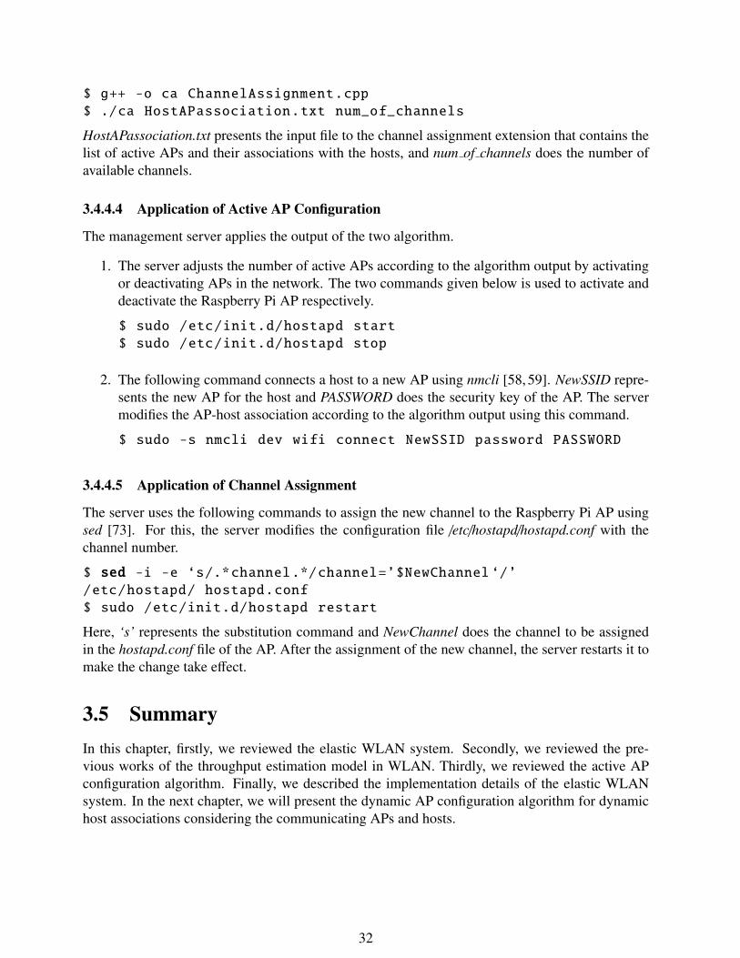
$ g++ -o ca ChannelAssignment.cpp

$ ./ca HostAPassociation.txt num_of_channels

HostAPassociation.txt presents the input file to the channel assignment extension that contains thelist of active APs and their associations with the hosts, and num of channels does the number ofavailable channels.

3.4.4.4 Application of Active AP Configuration

The management server applies the output of the two algorithm.

1. The server adjusts the number of active APs according to the algorithm output by activatingor deactivating APs in the network. The two commands given below is used to activate anddeactivate the Raspberry Pi AP respectively.

$ sudo /etc/init.d/hostapd start

$ sudo /etc/init.d/hostapd stop

2. The following command connects a host to a new AP using nmcli [58, 59]. NewSSID repre-sents the new AP for the host and PASSWORD does the security key of the AP. The servermodifies the AP-host association according to the algorithm output using this command.

$ sudo -s nmcli dev wifi connect NewSSID password PASSWORD

3.4.4.5 Application of Channel Assignment

The server uses the following commands to assign the new channel to the Raspberry Pi AP usingsed [73]. For this, the server modifies the configuration file /etc/hostapd/hostapd.conf with thechannel number.

$ sed -i -e ‘s/.*channel.*/channel=’$NewChannel ‘/’/etc/hostapd/ hostapd.conf

$ sudo /etc/init.d/hostapd restart

Here, ‘s’ represents the substitution command and NewChannel does the channel to be assignedin the hostapd.conf file of the AP. After the assignment of the new channel, the server restarts it tomake the change take effect.

3.5 SummaryIn this chapter, firstly, we reviewed the elastic WLAN system. Secondly, we reviewed the pre-vious works of the throughput estimation model in WLAN. Thirdly, we reviewed the active APconfiguration algorithm. Finally, we described the implementation details of the elastic WLANsystem. In the next chapter, we will present the dynamic AP configuration algorithm for dynamichost associations considering the communicating APs and hosts.

32

Chapter 4

Dynamic Active AP Configuration

In this chapter, we present the extension of the active AP configuration algorithm for dynamicbehaviors of joining and leaving hosts. Firstly, we describe the motivation of our proposal. Sec-ondly, we describe some related works. Thirdly, we present the algorithm extension for join andleave operations considering the currently communicating APs and hosts. Fourthly, we evaluatethe proposal through simulations using two networks topologies. Fifthly, we present the imple-mentation of the proposal in the elastic WLAN system testbed. Finally, we evaluate our proposalusing testbed experiments.

4.1 IntroductionIn Chapter 3, we reviewed the previous studies of the active AP configuration algorithm for theelastic WLAN system. This algorithm can optimize the number of active APs depending on trafficdemands and network situations [9, 10]. Unfortunately, this algorithm can find the solution for thefixed user state of the network, although user hosts often repeat joining and leaving the network.

To solve this issue, we propose the extension of the active AP configuration algorithm in orderto deal with this dynamic nature. By considering the currently communicating hosts and APs, thealgorithm can find the new configuration for host joining and leaving operations in the network.

4.2 MotivationThe active AP configuration algorithm consists of three phases, namely, the active AP and asso-ciated host selection phase, the channel assignment phase, and the channel load averaging phase.In the first phase, the algorithm selects the active APs and the host associations based on the statichost information in the system. In this phase, the algorithm selects the minimum number of activeAPs that can satisfy the predefined throughput constraints on the hosts. In the second phase, itassigns one channel to each active AP from the limited number of the non-interfered channels inorder to minimize the overall interference of the network. Finally, in the third phase, the channelloads are averaged by changing associated APs for hosts when their loads are high.

In a real WLAN system, hosts often join and leave from the network and the number of hostsusually fluctuate depending on the time and days of the week. Thus, the network configurationshould be adaptive for the dynamic nature of host joining and leaving. Also, some hosts maycurrently send or receive data to/from the Internet. Thus, their services should not be stoppedwhen a new configuration is composed.

33

4.3 Drawbacks of the Previous AlgorithmUnfortunately, the previous active AP configuration algorithm can find a solution for the fixed userstate in the network, although it is usual that users repeat joining and leaving the network. Even forany single join or leave operation, the algorithm may generate a totally new configuration withoutconsidering the current state. Thus, it cannot provide continuous services to the currently com-municating hosts. The new network configuration must avoid this discontinuity of communicationservices.

4.4 ContributionsIn this chapter, we first propose the extension of the active AP configuration algorithm to overcomethe discontinuity problem of the algorithm. The algorithm can handle the dynamic host behaviorby considering the rapid host join and leave operation. Figure 4.1 shows the dynamic extension ofthe previous algorithm. It takes the current network association as the input and finds the currentlycommunicating APs and hosts those are exchanging the data using Internet. Then, it finds thejoining or leaving hosts in the network. Finally, depending on the join or leave operation, thealgorithm finds the new configuration. In this extension, the currently communicating APs andhosts are designated as communicating APs and communicating hosts for convenience. Then, asthe new constraints, any communicating AP must not be deactivated and any communicating hostmust not change the associated AP by the algorithm.

Phase-2: Channel Assignment

Phase-1: Activate APs and Host

Association

Output

Phase-3: Load Averaging

Input

Dynamic Extension

Find Joining Host

Find Leaving Host

Find Communicating AP and Host

Apply Algorithm Extension

Figure 4.1: Dynamic active AP Configuration Algorithm extension operation flow.

Furthermore, the proposed algorithm extension is implemented on the elastic WLAN systemtestbed to verify the practicality in the real system. In this testbed implementation, Raspberry Piis adopted for the AP and Linux PC is for the host.

4.5 Related WorksIn this section, we briefly introduce related works in literature to this work.

34

[4] adopts a game theoretic approach to balance the loads among the APs. That is, the usersassociated with highly congested APs will be moved to less loaded APs for better throughputs.Although this approach can balance the loads among APs, the user movement from one AP toanother AP makes it impractical in real applications, because a host has to discover another suitableAP and move to the place, if it doesn’t succeed in receiving the required data rate or service fromthe associated AP.

[74, 75] propose a load balancing approach among APs to mitigate congestions and fair distri-butions of users. Each host monitors the wireless channel qualities that it experiences from nearbyAPs and reports them to the network control center that determines the host and AP associations.Since the objective function of the proportional fairness is non-linear, its implementation is muchmore challenging, where detecting the bottleneck users and finding their normalized bandwidthare NP-hard.

[76] provides an algorithm to place several extension points for cellular networks such that thethroughput capacity of WLAN is maximized. These extension points act as relay points betweenthe APs and the hosts located at longer distances. Each extension point can receive the packetsfrom the APs and deliver them to the hosts. In a conventional WLAN, the extension point is notused, because the multi-hop communications degrade the performance due to strong interferencesamong multi-hop links.

[77] presents an AP association approach to improve the network throughput while balancingthe loads among APs. The authors investigate and evaluate a measurement driven frameworkwith three objective functions in a dense WLAN; (i) the frequency/channel selection across theAPs to minimize the noise or interference between neighboring APs, (ii) the user association byconsidering the load of the AP and the receiving signal strength, and (iii) the power control for eachAP. While each of the three objective functions achieves its optimization objective individually, incertain cases, to apply all of them (channel selection, user association, and power control) willlead to the suboptimal performance. Moreover, the authors found that if all of them are randomlyapplied, it will degrade the performance. A host is initially associated with the AP that providesthe highest received signal strength indicator (RSSI). Then, any host from an overloaded AP ismigrated to a lightly loaded AP for balancing the load in the network.

[78] introduces a heuristic algorithm for the AP placement based on the user distribution onan indoor WLAN system. The authors have proposed a fuzzy C-clustering-based AP deploymentstrategy to maximize the user coverage and balance the load among the APs.

[79] examines an AP selection algorithm to maximize the throughput for a newly joining hostin the multi-rate WLAN by moving the host towards the location of the desired AP.

[80–82] focus on the highest RSSI to select the AP association. However, the AP with thehighest RSSI can be overloaded by a number of users, and thus, may not ensure the proper loadbalancing among APs.

[83] presents a smart AP solution to balance the loads across multiple Wi-Fi interfaces. Still,the implementation of this approach is difficult, since each AP must be equipped with multipleinterfaces operating on different channels simultaneously.

4.6 Extension of Active AP Configuration AlgorithmIn this section, we present the extension of the active AP configuration algorithm to consider thecurrently communicating APs and hosts.

35

4.6.1 Definitions of TermsIn the extension, any communicating host must not change the associated AP to ensure the con-tinuous Internet service, while any communicating AP must not be deactivated. For the algorithmextension, we introduce the following terms to describe the states of the network and simulations:

• joining host is a host that newly joins the network to be associated with an active AP for theInternet access. The algorithm must find the associated active AP for the joining host.

• leaving host is a host that leaves the network after completing the Internet service.

• communicating host is a host that is currently communicating with the Internet. The algo-rithm cannot change the associated AP to avoid the communication suspension.

• communicating AP is an AP that is currently associated with a communicating host. Thealgorithm cannot stop this AP to avoid the communication suspension.

• active host is a host that is currently associated with an active AP.

• inactive host is a host that is not associated with an active AP.

4.6.2 Joining Host OperationFirst, we present the algorithm extension for one joining host. When a new host joins the network,the associated active AP must be selected for the joining host such that the constraints in subsec-tion 3.3.1 are satisfied. Here, the selected active AP must satisfy the minimum host throughputconstraint when the following normalized link speed is considered if Ba < Be:

s jk = s jk ×Ba

Be (4.1)

where Ba and Be represent the available and expected total bandwidth respectively, s jk representsthe link speed between the jth AP and the kth host, and s jk does its normalized link speed. Then,the average host throughput (T H j) using the normalized link speeds is calculated for each activeAP ( jth AP) when the joining host is associated with it:

T H j =1∑

k

1s jk

(4.2)

where T H j represents the average host throughput for the jth AP. If T H j ≥ G, the minimum hostthroughput constraint is satisfied, where G represents the threshold for this constraint. If multipleactive APs can satisfy it, the AP that maximizes the E2 defined in Eq. (3.10) is selected. Onthe other hand, if any active AP cannot satisfy the constraints for the joining host, this host isfirst associated with the active AP that maximizes the E2 defined in Eq. (3.10), and the active APconfiguration algorithm in the previous chapter is applied from AP Selection Optimization (Step(4) in Section 3.3.2.1).

Here, to avoid the suspensions of the currently communicating hosts, the two modifications areincorporated: 1) any communicating AP is not deactivated in AP Selection Optimization, and 2) anycommunicating host does not change the associated active AP in Host Association Improvement(Step (3) in Section 3.3.2.1) and in AP Selection Optimization (Step (4) in Section 3.3.2.1).

36

4.6.3 Leaving Host OperationNext, we present the algorithm extension for one leaving host. When an existing host leaves thenetwork, it is only necessary to remove this leaving host from the associated active AP. Then, ifthe AP is not associated with any host, this AP is deactivated. Otherwise, to minimize the numberof active APs and improve the host associations, the active AP configuration algorithm is appliedfrom AP Selection Optimization (Step (4) in Section 3.3.2.1) with the two modifications for thejoining host.

4.6.4 Examples of Host Join OperationIn this paper, it is assumed that at most one host may join or leave the network at each time. First,the host join operation in Figure 4.2 is discussed. When H4 joins the network, it newly activatesAP2 to satisfy the minimum host throughput constraint. Then, to balance the loads between AP1and AP2, H2 changes the associated AP from AP1 to AP2, because H3 cannot change the associ-ated AP as the communicating host.

AP1AP2

H1

H2

H3

H4

(a) Before H4 join

AP1

H1

H2

H3

AP2

H4

(b) After H4 join

Figure 4.2: Host join operation.

4.6.5 Examples of Host Leave OperationThen, the host leave operation in Figure 4.3 is discussed. When H4 leaves the network, if H3changes the associated AP to AP1, it can deactivate AP2 while satisfying the minimum hostthroughput constraint. However, H3 cannot change the associated AP as the communicating host,and AP2 cannot be deactivated.

AP1

H2

H3

AP2

H1

H4

(a) Before H4 leave

AP1

H2

H3

AP2

H1

(b) After H4 leave

Figure 4.3: Host leave operation.

37

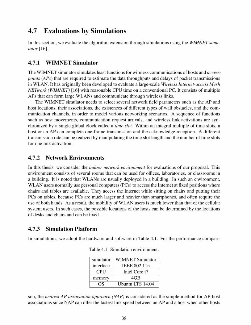
4.7 Evaluations by SimulationsIn this section, we evaluate the algorithm extension through simulations using the WIMNET simu-lator [16].

4.7.1 WIMNET SimulatorThe WIMNET simulator simulates least functions for wireless communications of hosts and access-points (APs) that are required to estimate the data throughputs and delays of packet transmissionsin WLAN. It has originally been developed to evaluate a large-scale Wireless Internet-access MeshNETwork (WIMNET) [16] with reasonable CPU time on a conventional PC. It consists of multipleAPs that can form large WLANs and communicate through wireless links.

The WIMNET simulator needs to select several network field parameters such as the AP andhost locations, their associations, the existences of different types of wall obstacles, and the com-munication channels, in order to model various networking scenarios. A sequence of functionssuch as host movements, communication request arrivals, and wireless link activations are syn-chronized by a single global clock called a time slot. Within an integral multiple of time slots, ahost or an AP can complete one-frame transmission and the acknowledge reception. A differenttransmission rate can be realized by manipulating the time slot length and the number of time slotsfor one link activation.

4.7.2 Network EnvironmentsIn this thesis, we consider the indoor network environment for evaluations of our proposal. Thisenvironment consists of several rooms that can be used for offices, laboratories, or classrooms ina building. It is noted that WLANs are usually deployed in a building. In such an environment,WLAN users normally use personal computers (PCs) to access the Internet at fixed positions wherechairs and tables are available. They access the Internet while sitting on chairs and putting theirPCs on tables, because PCs are much larger and heavier than smartphones, and often require theuse of both hands. As a result, the mobility of WLAN users is much lower than that of the cellularsystem users. In such cases, the possible locations of the hosts can be determined by the locationsof desks and chairs and can be fixed.

4.7.3 Simulation PlatformIn simulations, we adopt the hardware and software in Table 4.1. For the performance compari-

Table 4.1: Simulation environment.

simulator WIMNET Simulatorinterface IEEE 802.11n

CPU Intel Core i7memory 4GB

OS Ubuntu LTS 14.04

son, the nearest AP association approach (NAP) is considered as the simple method for AP-hostassociations since NAP can offer the fastest link speed between an AP and a host when other hosts

38

are not associated with the AP, where the active APs are selected by our algorithm. Table 4.2summarizes the simulation parameters that are used for the simulation using WIMNET simulator.

Table 4.2: Simulation parameters for WIMNET simulator.

parameter valuespacket size 2360 bytesmax. transmission rate 150 Mbit/spropagation model log distance path loss modelrate adaptation algorithm link speed estimation model [9]carrier sense threshold −85 dBmcollision threshold 10RTS/CTS yes

4.7.4 Host Behavior ModelIn our simulations, it is assumed that a host randomly joins and leaves the network by followingthe Poission distribution, and a host continues the communication with the Internet during the timederived by the Exponential distribution. In each simulation in this paper, at the first, N1 hosts arerandomly selected from all the N hosts in the network for N1 < N as active hosts, and the originalactive AP configuration algorithm is applied to the N1 active hosts so that the active APs and theassociated active hosts are obtained. For each active host, the communication duration time iscalculated by the following equation:

F(p, µ) =−ln(1 − p)

µ(4.3)

where p is 0−1 random number and µ is the parameter for the Exponential distribution. Then, everytime the constant time Td is elapsed, the communicating host is maintained if the communicationduration time is not over since the arrival to the network. Here, Td = 10sec is used in this paper.Besides, the number of newly joining hosts from inactive hosts and the number of leaving hostsfrom active hosts are calculated here by the following procedure:

1. Calculate the probability to select each number k by the Poission distribution:

F(k, λ) =λke−λ

k!, (4.4)

where λ is the parameter for the Poission distribution.

2. Calculate the cumulative probability C (k, λ) for each number k by:

C (k, λ) =

k∑i=0

λi · e−λ

i!(4.5)

3. Generate a 0 − 1 random number p.

4. Find k such that C (k, λ) ≤ p < C (k + 1, λ).

Then, the corresponding number of joining hosts are randomly selected from inactive hosts. Foreach newly joining host, the communication duration time is calculated by Eq. (4.3).

39

4.7.5 Evaluation of Small TopologyFirstly, we evaluate our proposal using a small-size network topology.

4.7.5.1 Small Topology

The small topology in Figure 4.4 is first considered for simulations, where 30 hosts, 4 DAPs aredistributed in the 100m × 50m rectangular area. The circles and squares represent the APs andhosts respectively. The minimum host throughput threshold G = 10Mbps and the bandwidth limitconstraint Ba = ∞ are examined. As the host behavior model in this topology, N1 = 18 hosts arerandomly selected as initial active hosts from N = 30 hosts, and λ = 1 and µ = .02 are adopted.

Active host Inactive host Com. active host

Active AP Inactive AP Com. active AP

CH1

CH6

Figure 4.4: Solution for small topology with 30 hosts and 4 APs.

4.7.5.2 Results

Figure 4.5 (a) shows the changes of the number of active hosts and the number of communicatingactive APs by the host behavior model, the number of active APs by the proposed algorithm, andthe least number of APs required to satisfy the minimum host throughput constraint (ideal APs),when the simulation time elapsed. The number of ideal APs is calculated by G × N1/AT . ATrepresents the average total throughput for one AP that is given by the throughput at the averageleast distance with each host in the network. This graph indicates that the number of active APs isdynamically controlled by the proposed algorithm depending on the number of active hosts.

Figure 4.5 (b) shows the changes of the minimum host throughput and the overall throughput bythe WIMNET simulator for the AP-host association by the proposal and for that by the comparedNAP. This graph indicates that the minimum host throughput by the proposal is always largerthan the threshold G = 10Mbps whereas that by the comparison is sometimes smaller than thethreshold. Besides, the overall throughput by the proposal is larger than that by the comparison atmost of the simulation time.

40

10 20 30 40 50 60 70 80 90 10012

14

16

18

20

22

24

26

# of active hosts # of ideal APs # of active APs # of com. active APs

Simulation time (sec)

# o

f act

ive

host

s

0

1

2

3

4

5

6

# of

act

ive

AP

s , c

om. a

ctiv

e A

Ps

and

idea

l AP

s

(a) Change of active hosts and APs.

10 20 30 40 50 60 70 80 90 1004

6

8

10

12

14

16 Min. host Throgh. of proposed alg. Min. host throgh. of nearest alg. Overall throgh. of proposed alg. Overall throgh. of nearest alg.

Simulation Time (sec)

Min

. hos

t thr

ough

put (

Mbp

s)

200

250

300

350

400

450

500

550

600

Ove

rall

thro

ughp

ut (M

bps)

(b) Change of min. host and overall throughputs.

Figure 4.5: Performance graph for small topology.

Table 4.3 compares the average minimum host throughput and overall throughput by the twomethods. This table also indicates that the performance by the proposal is better than that by thecomparison.

4.7.6 Evaluation of Large TopologySecondly, we evaluate our proposal using a large-size network topology.

41

Table 4.3: Throughput comparison between two methods for both topology.

instance small topology large topologymethod proposed compare proposed compareave. min. host throughput (Mbps) 12.21 10.51 11.53 10.31ave. overall throughput (Mbps) 301.81 261.47 450.70 407.69

4.7.6.1 Large Topology

The large topology in Figure 4.6 is then considered for simulations, which basically models thethird floor of Engineering Building-2 in Okayama University. 70 hosts and 10 DAPs are regularlydistributed in the six rooms with two different sizes, 7m × 6m and 3.5m × 6m. The same minimumhost throughput constraint G = 10Mbps and bandwidth limit constraint Ba = ∞ are examined.As the host behavior model in this topology, N1 = 35 hosts are randomly selected as initial activehosts from N = 70 hosts, and λ = 1.5 and µ = .02 are adopted.

Room D301 Room D302 Room D303

Room D304 Room D305 Room D306

Active AP Inactive AP Com. active AP

Active host Inactive host Com. active host

CH6CH11

CH6

CH1

Figure 4.6: Solution for large topology with 70 hosts and 10 APs.

4.7.6.2 Results

Figure 4.7 (a) shows the changes of the number of active hosts and the number of communicat-ing active APs by the host behavior model, and the number of active APs by the proposed algo-rithm, when the simulation time elapsed. Figure 4.7 (b) shows the changes of the minimum hostthroughput and the overall throughput by the WIMNET simulator for the AP-host association bythe proposal and for that by the compared NAP. From them, the same performance results can beobserved for the large topology as for the small topology.

42

10 20 30 40 50 60 70 80 90 1000

10

20

30

40

50

# of active hosts # of ideal APs # of active APs # of com. active APs

Simulation time (sec)

# o

f act

ive

host

s

2

3

4

5

6

# of

act

ive

AP

s , c

om. a

ctiv

e A

Ps

and

idea

l AP

s

(a) Change of active hosts and APs.

10 20 30 40 50 60 70 80 90 1000

2

4

6

8

10

12

14

16 Min. host Throgh. of proposed alg. Min. host throgh. of nearest alg. Overall throgh. of proposed alg. Overall throgh. of nearest alg.

Simulation Time (sec)

Min

. hos

t thr

ough

put (

Mbp

s)

250

300

350

400

450

500

550

600

650

700

750

800

Ove

rall

thro

ughp

ut (M

bps)

(b) Change of min. host and overall throughputs.

Figure 4.7: Performance graph for small topology.

4.7.6.3 Results for Larger λ

In some networks, the number of users can be more widely fluctuated by time. For example, atpublic WLANs in a station or an airport, a lot of users may arrive there by a train or an airplaneand join the network at the same time. They often stay there for a short time. To simulate suchcases, the larger value of λ = 4, 5 and µ = .05 are adopted. Figures 4.8 (a) and 4.9 (a) showthe changes of the number of active hosts and the number of communicating active APs and thenumber of active APs for each λ respectively. Figures 4.8 (b) and 4.9 (b) indicate that by theproposal, the minimum host throughput is always larger than the threshold G = 10Mbps and the

43

10 20 30 40 50 60 70 80 90 1000

10

20

30

40

50

60

# of active hosts # of ideal APs # of active APs # of com. active APs

Simulation time (sec)

# o

f act

ive

host

s

2

4

6

8

10

# of

act

ive

AP

s , c

om. a

ctiv

e A

Ps

and

idea

l AP

s

(a) Change of active hosts and APs.

10 20 30 40 50 60 70 80 90 1006

8

10

12

14

16

18

20 Min. host Throgh. of proposed alg. Min. host throgh. of nearest alg. Overall throgh. of proposed alg. Overall throgh. of nearest alg.

Simulation Time (sec)

Min

. hos

t thr

ough

put (

Mbp

s)

400

600

800

1000

1200

1400

Ove

rall

thro

ughp

ut (M

bps)

(b) Change of min. host and overall throughputs.

Figure 4.8: Performance graph for large topology with λ = 4.

overall throughput is larger than that of the comparison. Table 4.4 compares the average minimumhost throughput and overall throughput between the two methods. This table indicates that theperformance by the proposal is better than that by the comparison.

4.7.6.4 Results for Moving Hosts

As described before, this study assumes that WLAN users usually use PCs on fixed positions wheredesks or chairs are available. However, users may move to different positions in the network field ifthe new positions are better for users. This move of a host to a different position can be representedby a pair of the leave operation from the current position and the join operation at the new position.

44

10 20 30 40 50 60 70 80 90 10010

20

30

40

50

60

70 # of active hosts # of ideal APs # of active APs # of com. active APs

Simulation time (sec)

# of

act

ive

host

s

2

4

6

8

10

# of

act

ive

AP

s , c

om. a

ctiv

e A

Ps

and

idea

l AP

s

(a) Change of active hosts and APs.

10 20 30 40 50 60 70 80 90 100

2

4

6

8

10

12

14

16

18

20

22 Min. host Throgh. of proposed alg. Min. host throgh. of nearest alg. Overall throgh. of proposed alg. Overall throgh. of nearest alg.

Simulation Time (sec)

Min

. hos

t thr

ough

put (

Mbp

s)

200

250

300

350

400

450

500

550

600

650

700

750

800

Ove

rall

thro

ughp

ut (M

bps)

(b) Change of min. host and overall throughputs.

Figure 4.9: Performance graph for large topology with λ = 5.

Table 4.4: Throughput comparison between two methods for large λ.

instance λ = 4 λ = 5method proposed compare proposed compareave. min. host throughput (Mbps) 12.65 10.16 14.33 11.70ave. overall throughput (Mbps) 525.39 441.21 478.29 387.73

Thus, when a host move appears, basically, the algorithm extension for a leaving host and that for ajoining host are applied sequentially. However, if the host moves to a near position from the current

45

one, it can keep the same associated AP if the minimum host throughput constraint is satisfied. Inthis case, the proposed extension is not applied, where only the link speed is updated.

To consider moving hosts, we simulated the proposal with them for the large topology. Here,λ = 1.5 is used for the parameter of joining and leaving hosts, µ = .02 is for the parameter ofthe communication duration time, and 10% is for the communicating host selection probability.At the time hosts may join or leave the network, the moving hosts are randomly selected fromnon-communicating hosts with the fixed probability, where 0%, 5%, 10%, and 15% are used forthis probability. The selected moving host is moved to a randomly selected host position instantly.

Table 4.5 summarizes the simulation results. The throughput performance is similar in anycase. Therefore, our proposal is effective for the moving hosts in the network field.

Table 4.5: Simulation results for moving hosts.

parameters resultsmoving host selection probability 0% 5% 10% 15%avg. # of active APs 4.54 4.54 4.58 4.54avg. # of moving hosts 0 1.86 3.70 5.40avg. # of communicating hosts 3.38 3.34 3.44 3.36avg. min. host throughput (Mbps) 11.32 11.16 11.34 11.33avg. overall throughput (Mbps) 452.44 448.22 446.95 443.50

4.7.6.5 Comparisons with Previous Study

To clarify the effectiveness of the proposed algorithm extensions, we simulate the cases when therate of the communicating hosts among the hosts is set to 25% and 50%, and compare the numberof the active APs, the minimum host throughput, the total throughput, and the number of hostschanging the associated APs between the previous algorithm and the proposed one. It is noted thatas the number of hosts changing the associated APs increases, the number of suspending hosts tochange the associated APs increases.

Table 4.6: Comparisons of performances between proposal and previous.

simulation cases resultsrate of com. host parameters proposal previous

25%avg. # of active APs 5.00 5.00avg. min. host throughput (Mbps) 10.96 10.97avg. overall throughput (Mbps) 487.45 480.81avg. rate of AP change hosts among com. hosts 0% 37.5 %

50%avg. # of active APs 6.00 6.00avg. min. host throughput (Mbps) 12.31 13.03avg. overall throughput (Mbps) 562.74 568.98avg. rate of AP change hosts among com. hosts 0% 41.2%

Table 4.6 shows the results when the rate of the communicating hosts is set to 25% and 50%.The network load is changed where the number of active hosts is set to 41 on average, to takethe average values of the minimum host throughput and the overall throughput for each case. Itis found that the average values of the both throughputs are similar between the two algorithms,

46

while 37.5% or 41.2% hosts must change the associated APs while communicating, which canincrease the network management overheads and suspend the Internet services for them.

4.7.6.6 Discussions

The simulation results show that at any situation, the extended algorithm can minimize the numberof active APs while the minimum host throughput is maintained, and the overall throughput isbetter than the nearest AP association approach. They confirm the effectiveness of the proposal.

10 15 20 25 30 35 40 45 50 55 60 65 70 75

10

20

30

40

50

# of active hosts # of ideal APs # of active APs # of com. active APs

Simulation time (sec)

# o

f act

ive

host

s

2

4

6

8

# of

act

ive

AP

s , c

om. a

ctiv

e A

Ps

and

idea

l AP

s(a) Change of active hosts and APs.

10 15 20 25 30 35 40 45 50 55 60 65 70 750

2

4

6

8

10

12

14

16 Min. host Throgh. of proposed alg. Min. host throgh. of nearest alg. Overall throgh. of proposed alg. Overall throgh. of nearest alg.

Simulation Time (sec)

Min

. hos

t thr

ough

put (

Mbp

s)

300

350

400

450

500

550

600

650

700

750

800O

vera

ll th

roug

hput

(Mbp

s)

(b) Change of min. host and overall throughputs.

Figure 4.10: Performance graph for large topology with network parameter change.

In Figure 4.5 (a), the number of active APs and the number of ideal APs are always same. In

47

others, they are sometimes different by 1 or 2 because of the communicating APs that cannot bedeactivated. Furthermore, in order to see the performance of the extended algorithm when impor-tant parameters in the host behavior model are changed during the simulation, another simulationis conducted, where Td is changed from 10sec to 5sec and λ is changed from 3 to 2 when 50sec iselapsed. As shown in Figure 4.10, our algorithm can adapt to the change of the network parametersimmediately.

The results in Section 4.7.6.5 show that our proposal can avoid the suspensions of communi-cating host due to the change of the associated APs. The host mobility results in Section 4.7.6.4also show that the proposed algorithm can improve the network performance similar to relatedwork [79]. Furthermore, by considering host leaving from the network, this algorithm deactivatesunnecessary APs to save energy and reduce interferences. On the whole, the proposed extensionexhibits dynamic feature of real time WLAN system and outperform all the other algorithms.

4.8 Testbed ImplementationIn this section, we present the implementation of the elastic WLAN system testbed using Rasp-berry Pi for the proposal. This testbed adopts a server to manage the information and control thesystem.

4.9 Execution Flow of Elastic WLAN for Dynamic ApproachFigure 4.11 shows the execution flow of the elastic WLAN system testbed. To deal with dynamicbehaviors of joining and leaving hosts, the four steps, Steps 7-10, are added to the six steps, Steps1-6, of the original implementation in [9]. Before starting the execution of Step 7 to Step 10, shownin Figure 4.11, the server compiles all the programs made by C at once to save the CPU time andthe load. The following commands perform the compilation of each program.

Linux commands for compilation of each C program� �#/bin/bash

# to detect the network change and identify joining or leaving host

01: g++ -o chkD CheckDevicesForjoinleave.cpp

02: g++ -o Inputforleavinghost GenAlgmInputforLeaving.cpp

03: g++ -o ckcurap CheckWithCurrentAP.cpp

04. g++ -o dcs Decisioncurjoin.cpp

05. g++ -o CrIn CreateInputforAllHost.cpp

06: g++ -o ckcomap Comaphost.cpp

07: g++ -o DAPC DAPC.cpp� �After that, the server uses the executable files and the necessary input files generated by each stepto perform the whole execution process. The following section describes how the server can detectcommunicating APs and hosts. Then, all the steps are describes with detail operations.

4.9.1 Detection of Communicating AP and HostThe AP association of any host that is currently communicating with the Internet, must be con-tinued. To detect such communicating APs and hosts, the server inspects the packets that are

48

Go t

o S

tep

7

1

8

9

10Application of Algorithm Output

Execution of Algorithm Extension

Leaving or Joining Host Identification

5

6

7Network Change Detection

Application of Channel Assignment

Application of Active AP Configuration

2

3

4Execution of Channel Assignment Algorithm

Execution of Active AP Configuration Algorithm

Generation of input for AP Configuration Algorithm

AP Configuration of Raspberry Pi

Figure 4.11: Elastic WLAN system execution flow for Dynamic active AP Configuration.

exchanged between the host and the AP, using tcpdump [84]. The tcpdump is a powerful networkdebugging tool and command-line packet analyzer on a network interface. The server collects thepackets between the active hosts and their associated active APs, and detects the hosts and APsthat are currently communicating from them. The following commands are used in this step:

Linux commands for communicating hosts and APs dectection� �#/bin/bash

# to inspect packets exchange between hosts and APs

01: timeout 50 tcpdump -i wlan0 host ip

# analyze and detect Com. APs and hosts

02: ./ckcomap tcppacket.txt� �The command in 01 inspects the TCP packets between the APs and their associated hosts for50sec. using tcpdump. Here, host ip represents the IP address of any host connecting to anyactive AP. Then, a C program is executed to filter and analyze the packets. The server detects thecommunicating hosts and APs using the command in 02.

4.9.2 Network Change DetectionIn this step, the server detects whether the network state is being changed due to joining of newhosts or leaving of existing hosts in the network. To detect it, the server uses the following com-mands:

49

Linux commands for network change detection� �#/bin/bash

# to explore the connected devices in network

01: sudoarp-scan --interface=eth0 192.168.11.0/24

# to detect the network change

02: ./chkD netoutpre.txt netoutrecent.txt� �The command in 01 explores the connected devices in the network using arp-scan [47]. The outputconsists of the IP and MAC addresses of the hosts and the APs that are available in the network.The command in 02 identifies network changes. Here, netoutpre.txt and netoutrecent.txt containthe device information of the network according to previous and current status. The C program willcheck the devices and can detect the network changes. After detecting the network state change,the server takes the following steps to control the number of active APs.

4.9.3 Leaving or Joining Host IdentificationAfter detecting the network state change, the server identifies the hosts that newly joined or leftthe network and finds their IP addresses by running the same C program.

Linux commands for leaving or joining host identification� �#/bin/bash

# identify joining or leaving hosts/hosts

01: ./chkD netoutpre.txt netoutrecent.txt� �The command in 01 takes the two files, netoutpre.txt and netoutrecent.txt, as the inputs. Afteranalyzing the IP and MAC addresses of the devices, the server identifies and prepares the list ofthe changed hosts. If there is no change in the network, the server goes back to the previous stepin Figure 4.11.

4.9.4 Execution of AlgorithmAccording the host identifications, the active AP configuration algorithm is applied for joininghosts or leaving hosts. The output of the algorithm contains the information of the networkchanges, including the associations between the hosts and APs and the list of APs for activation ordeactivation.

1. Steps in Leaving OperationBefore executing the algorithm for the leaving host, the server prepares the input by thefollowing commands:

Linux commands for leaving host operation� �#/bin/bash

# generate input for the Modified APC Alg.

01: ./Inputforleavinghost leavinghosts.txt

alg_out.txt previousinput.txt group_info.txt newinput.txt

#run the DAPC

02: ./DAPC newinput.txt min_host_throughput com.txt� �The command in 01 takes the input from previousinput.txt and prepares the new input for the

50

leaving host extension. Before applying the algorithm, the server detects the communicatinghosts and APs, as described in Section 4.9.1. After that, the extended active AP configurationalgorithm is executed using the command in 02 to finds the new configuration by consideringthe communicating APs and the hosts in com.txt detected in Section 4.9.1.

2. Steps in Joining OperationThe server collects the signal strengths of the newly joining hosts and the active APs in thenetwork. Then, it applies the following commands:

Linux commands for joining host operation� �#/bin/bash

# to inspect signal strength for joining host

01: sudo nm-tool

02: sh ./nm_scriptjoinhost.sh

03: ./ckcurap JoinHosts.txt

# decision on current APs

04: ./dcs ch_association.sh ap_activation.sh

# generate input for the Modified APC Alg

# if we need to activate new AP

05: ./CrIn CurHostsall.txt CurAPall.txt

#run the DAPC

06: ./DAPC newinput.txt min_host_throughput com.txt� �The commands in 01 and 02 find the receiving signal strength of each joining host fromevery AP using nm-tool [49, 50]. The ssh [53, 54] protocol is used to execute the commandin 01 remotely in each host. The output consists of the currently associated APs, the listof associable APs, and the receiving signal strength of each host from all the associableAPs. After this, the server converts the receiving signal strength to the estimated link speedusing the sigmoid function in [72], and generates the input for the active AP configurationalgorithm. By using the commands in 03 and 04, the server knows whether the currentlyactivated APs can satisfy the minimum host throughput constraint for the hosts or not. Italso detects the changes of their AP associations, if necessary. If they cannot satisfy theconstraint, the server applies the algorithm to activate some deactivated APs, after preparingthe algorithm input using the command in 05. Finally, the dynamic active AP configurationalgorithm is executed to find the association after the join operation using the command in06. Again, the communicating hosts and APs are detected using the procedure in Section4.9.1. Here, com.txt is the list of currently communicating hosts and APs.

4.9.5 Application of Algorithm OutputThen, the server changes the corresponding associations and deactivates all the unused APs byfollowing the algorithm output. For the joining hosts, some additional APs are activated and areassigned the channels, if necessary. Besides, the channels of some active APs are also changed, ifnecessary. The following commands are used in this step. The commands in 01 and 02 activateor deactivate the Raspberry Pi AP respectively. The server adjusts the number of active APsaccording to the algorithm output by activating or deactivating APs in the network. The commandin 03 connects a host to a new AP using nmcli [58, 59]. Here, NewSSID represents the new AP

51

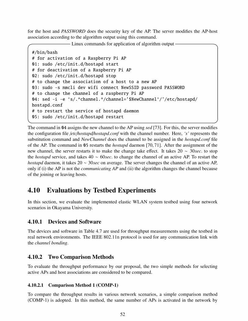
for the host and PASSWORD does the security key of the AP. The server modifies the AP-hostassociation according to the algorithm output using this command.

Linux commands for application of algorithm output� �#/bin/bash

# for activation of a Raspberry Pi AP

01: sudo /etc/init.d/hostapd start

# for deactivation of a Raspberry Pi AP

02: sudo /etc/init.d/hostapd stop

# to change the association of a host to a new AP

03: sudo -s nmcli dev wifi connect NewSSID password PASSWORD

# to change the channel of a raspberry Pi AP

04: sed -i -e ‘s/.*channel.*/channel=’$NewChannel‘/’/etc/hostapd/

hostapd.conf

# to restart the service of hostapd daemon

05: sudo /etc/init.d/hostapd restart� �The command in 04 assigns the new channel to the AP using sed [73]. For this, the server modifiesthe configuration file /etc/hostapd/hostapd.conf with the channel number. Here, ‘s’ represents thesubstitution command and NewChannel does the channel to be assigned in the hostapd.conf fileof the AP. The command in 05 restarts the hostapd daemon [70, 71]. After the assignment of thenew channel, the server restarts it to make the change take effect. It takes 20 ∼ 30sec. to stopthe hostapd service, and takes 40 ∼ 60sec. to change the channel of an active AP. To restart thehostapd daemon, it takes 20 ∼ 30sec on average. The server changes the channel of an active AP,only if (i) the AP is not the communicating AP and (ii) the algorithm changes the channel becauseof the joining or leaving hosts.

4.10 Evaluations by Testbed ExperimentsIn this section, we evaluate the implemented elastic WLAN system testbed using four networkscenarios in Okayama University.

4.10.1 Devices and SoftwareThe devices and software in Table 4.7 are used for throughput measurements using the testbed inreal network environments. The IEEE 802.11n protocol is used for any communication link withthe channel bonding.

4.10.2 Two Comparison MethodsTo evaluate the throughput performance by our proposal, the two simple methods for selectingactive APs and host associations are considered to be compared.

4.10.2.1 Comparison Method 1 (COMP-1)

To compare the throughput results in various network scenarios, a simple comparison method(COMP-1) is adopted. In this method, the same number of APs is activated in the network by

52

Table 4.7: Devices and software in the testbed.

Devices and software

server PCOS Ubuntu LTS 14.04model Lesance W255HUProcessor Intel(R), Core(TM)-i3

client PC (type-1)OS Ubuntu LTS 14.04Model Toshiba Dynabook R731/BProcessor Intel(R), Core-i5

client PC (type-2)OS Ubuntu LTS 14.04Model Fujitsu Lifebook S761/C/SSDProcessor Intel(R), Core-i5

access pointRaspberry Pi 3

OS RaspbianProcessor 1.2 GHz

software/tools

openssh to access remote PC and APhostapd to prepare and configure APnmcli for association changenm-tool to measure signal strengthtcpdump to analyze packetsarp-scan to discover active network devices

randomly selecting them from available APs, where the channel is assigned by our algorithm. Forany newly joining host, the host is associated with the AP that provides the highest RSSI from theactive APs.

4.10.2.2 Comparison Method 2 (COMP-2)

As another comparison method (COMP-2), the active APs are also selected by the RSSI to thejoining host. For any joining host, if the number of active APs is smaller than the algorithm, theAP that provides the highest RSSI is newly activated, and the host is associated with it. Again, forany AP, the channel is assigned by the algorithm.

4.10.3 Network ScenariosFor evaluations, four network scenarios are prepared for the elastic WLAN system testbed. Foreach AP, one of the three orthogonal channels, 1, 6, and 11, is assigned by the proposed algorithm.

4.10.3.1 3 × 4 Scenario in One Room

In the first scenario, three Raspberry Pi devices for APs and four Linux PCs for hosts are preparedin a room of size 7m× 6m. Figure 4.12 shows the distance between the hosts and APs. Any accesspoint is connected to the server using the wired connection.

53

H3

H1

2m

2m

3m

H2

H4

AP1

AP2

AP3

Figure 4.12: Testbed for 3 × 4 scenario in one room.

4.10.3.2 3 × 4 Scenario in Different Rooms

In the second scenario, three Raspberry Pi devices for APs and four Linux PCs for hosts areprepared in two rooms with the size of 7m × 6m separated by the wall and one corridor at thethird floor of Engineering Building-2 in Okayama University. As shown in Figure 4.13, any AP is5m − 6m away from another AP in the different room and corridor to reduce the interference.

H1

AP1

H2

AP2

H4

H3

AP3

Figure 4.13: Testbed for 3 × 4 scenario in different rooms.

4.10.3.3 3 × 6 Scenario

In the third scenario, three Raspberry Pi devices for APs and six Linux PCs for hosts are placed inthe same field, as shown in Figure 4.14.

54

H1

AP1

H2

AP2

H5

H3

AP3

H4

H6

Figure 4.14: Testbed for 3 × 6 scenario.

4.10.3.4 4 × 8 Scenario

In the fourth scenario, four Raspberry Pi devices for APs and eight Linux PCs for hosts are dis-tributed in the three rooms and the corridor as shown in Figure 4.15 at the second floor of GraduateSchool Building in Okayama University. The size of each room is 9m × 5.5m, 3.5m × 5.5m, and7m × 5.5m respectively. Any AP is 4m away from another AP in the same room.

H7

AP4

H8

H5

H1

AP3

H3

H2AP2

H6

AP1

H4

Figure 4.15: Testbed for 4 × 8 scenario.

4.10.4 Host Join/Leave DynamicsIn each scenario, the host join/leave dynamics in the network are represented by a sequence ofstages. At each stage, 1) one host joins or leaves the network, 2) Steps 7-10 in Section 4.9 areexecuted, and 3) the throughputs of all the active hosts are measured when they are concurrently

55

communicating with the iperf [24] server through the associated APs. By following the host be-havior model in 4.7.4, the joining and leaving hosts are randomly selected for each network stagewith λ = 1 and µ = .02.

4.10.5 Throughput Measurement ResultsFor each scenario, the throughputs at each stage are measured and compared.

4.10.5.1 3 × 4 Scenario in One room

Figure 4.16 (a) and (b) show the minimum host throughput results and the overall throughputresults in the testbed for the 3 × 4 scenario in one room, by the proposal, by COMP-1, and byCOMP-2 at each stage, where the number of active hosts is changed from 1 to 4. Except for theminimum host throughput at stage 4, our proposal always provides the better performance thanCOMP-1.

1 2 3 4 5 60

5

10

15

20

25

30

35

40

Min

. hos

t thr

ough

put (

Mbp

s)

Network Stages

DAPC COMP-1 COMP-2

(a) Minimum host throughput.

1 2 3 4 5 60

20

40

60

Ove

rall

thro

ughp

ut (M

bps)

Network Stages

DAPC COMP-1 COMP-2

(b) Overall throughput.

Figure 4.16: Throughput results for 3 × 4 scenario in one room.

4.10.5.2 3 × 4 Scenario in Different Rooms

Figure 4.17 (a) and (b) show the minimum host throughput results and the overall throughputresults in the testbed for the 3 × 4 scenario in different rooms, by the proposal, by COMP-1, andby COMP-2 at each stage, where the number of active hosts is changed from 1 to 4. Except forthe minimum host throughput at stages 3, 5 and the overall throughput at stage 3, our proposalalways provides the better performance than COMP-1 and COMP-2. It can be observed that theminimum host throughput becomes lower at any stage than that in one room case. Here, since ahost is connected to an AP in a different room, the RSS at such a host from the AP becomes smallerdue to the wall attenuation, and thus, the throughput becomes lower.

4.10.5.3 3 × 6 Scenario

Figure 4.18 (a) and (b) show the minimum host throughput results and the overall throughputresults in the testbed for the 3 × 6 scenario, by the proposal, by COMP-1, and by COMP-2 at

56

1 2 3 4 5 60

5

10

15

20

25

30

35

Min

. hos

t thr

ough

put (

Mbp

s)

Network Stages

DAPC COMP-1 COMP-2

(a) Minimum host throughput.

1 2 3 4 5 60

10

20

30

40

50

60

70

Ove

rall

thro

ughp

ut (M

bps)

Network Stages

DAPC COMP-1 COMP-2

(b) Overall throughput.

Figure 4.17: Throughput results for 3 × 4 scenario in different rooms.

each stage, where the number of active hosts is changed from 2 to 6. Except for the minimumhost throughput at stage 1, our proposal always provides the better performance than COMP-1 andCOMP-2.

1 2 3 4 5 60

2

4

6

8

10

12

Min

. hos

t thr

ough

put (

Mbp

s)

Network Stages

DAPC COMP-1 COMP-2

(a) Minimum host throughput.

1 2 3 4 5 60

20

40

60

80

Ove

rall

thro

ughp

ut (M

bps)

Network Stages

DAPC COMP-1 COMP-2

(b) Overall throughput.

Figure 4.18: Throughput results for 3 × 6 scenario.

4.10.5.4 4 × 8 Scenario

As the largest topology, Figure 4.19 (a) and (b) show the minimum host throughput results and theoverall throughput results in the testbed for the 3 × 6 scenario, by the proposal, by COMP-1, andby COMP-2 at each stage, where the number of active hosts is changed from 3 to 8. Except forthe minimum host throughput at stage 1, our proposal always provides the better performance thanCOMP-1 and COMP-2.

57

1 2 3 4 5 60

2

4

6

8

Min

. hos

t thr

ough

put (

Mbp

s)

Network Stages

DAPC COMP-1 COMP-2

(a) Minimum host throughput.

1 2 3 4 5 60

20

40

60

80

100

120

Ove

rall

thro

ughp

ut (M

bps)

Network Stages

DAPC COMP-1 COMP-2

(b) Overall throughput.

Figure 4.19: Throughput results for 4 × 8 scenario.

4.11 SummaryIn this chapter, firstly, we described the motivation of our proposal. Secondly, we described somerelated works. Thirdly, we presented the extension of the active AP configuration algorithm fordynamic host joining and leaving. Fourthly, we evaluated the proposal through simulations usingthe WIMNET simulator. Fifthly, we described the implementation of the proposal in the elasticWLAN system testbed. Finally, we evaluated our proposal through experiments using the testbed.In the next chapter, we will present the security update functions for the elastic WLAN system.

58

Chapter 5

System Security Implementation in elasticWLAN Testbed

In this chapter, we describe the implementations of the two security functions for the elastic WLANsystem testbed: the system software update function and the user authentication function. We alsoconfirm the correctness of them through experiments.

5.1 MotivationIn the current implementation of the elastic WLAN system, we limit a Linux PC for a host andthe server, and choose Raspberry Pi for an AP. Since all the host PCs and the APs are usingthe same platform, it is important to keep the system software updated for the latest version formaintaining the operational availability, confidentiality and integrity. Basically the majority ofcyber-attacks target known vulnerabilities in the system software. Any software vulnerability isone of the security hole found in a software program or operating system. Thus, the managementof the system software updates has become a serious challenge for modern organizations.

To increase the security and performance of the system, it is important to keep updating thesystem and application software to the latest version. Here, to reduce the overhead in downloadingthe software files from the Internet, a local repository server is prepared to download and storeall the updated files and packages periodically from the original repository and to distribute themto the APs and the hosts. The user authentication is also inevitable to enhance the security of thesystem.

In this study, we implement the system software update function and the user authenticationfunction in the elastic WLAN system. The system software update function identifies the newestversion of the system and application software that have been installed into the AP and the hostin the system. This function periodically checks the version for each software in the originalrepository in the Internet. Then, if the newer version exists, it downloads the necessary files toupdate the software, and stores them in the prepared local repository server. Every AP and userhost in the system accesses to this server to update the system software.

The user authentication function is implemented using the RADIUS server. Any newly join-ing user to the system must register the information for authentication at the server. Using thisinformation, the server authenticates the joining host user by sending the authentication messagevia one AP in the system to the server. Through experiments, we confirm the correctness of theseimplemented functions.

59

5.2 Importance of System Software UpdateThe system software update function is implemented based on the following observations:

• Security:Hackers may be always finding new ways to attack a system by finding security holes of thesoftware in the system. The regular update of the software can remove the known securityholes.

• Functionality:The latest software often provides new features and running speed enhancements.

• Load:The use of the local repository server can reduce the bandwidth required to download the filesfrom the original repository in the Internet. It can be very helpful in developing countriesincluding Bangladesh and Myanmar suffering from the unreliable and slow Internet access.

5.3 Implementation of System Software Update FunctionIn this section, we present the implementation of the system software update function in the elasticWLAN system testbed.

5.3.1 Configuration of Local Repository ServerThe configuration of the local repository server for the system software update function is de-scribed in details here. This server stores the latest files and packages for the system softwarelocally inside the elastic WLAN system. A Linux PC is used for this server. The apt-mirror tool isused to mirror or copy any part (or even all) of Ubuntu GNU/Linux distributions and any other aptsource provided by an open source developer [85]. The following commands are used to configurethe server with apt-mirror:

1. sudo apt-get install apt-mirror

2. cd /var/spool/apt-mirror

3. mkdir var mirror skel

4. sudo nano /etc/apt/mirror.list

5. sudo apt-mirror

The command in (1) is used to install apt-mirror to the local server. The commands in (2) and (3)create the necessary folder to store the files, so that this repository server works correctly. Then,apt-mirror is configured to collect the necessary files from the original repository. The commandin (4) is used to edit the source list of mirror.list file. Here, we put the source address of the originalmirror site for the Raspbian OS. From this site, apt-mirror downloads all the packages and files.Figure 5.1 shows an example mirror.list file. Finally, the command in (5) allows the server todownload the system files and packages to be stored in this server.

60

############# config #################### set base_path /var/spool/apt-mirror## set mirror_path $base_path/mirror# set skel_path $base_path/skel# set var_path $base_path/var# set cleanscript $var_path/clean.sh# set defaultarch <running host architecture># set postmirror_script $var_path/postmirror.sh# set run_postmirror 0set nthreads 20set _tilde 0############### end config ##############

deb-armhf http://mirrordirector.raspbian.org/raspbian/ jessie main contrib non-free rpi

deb-src http://mirrordirector.raspbian.org/raspbian/ jessie main contrib non-freeclean http://mirrordirector.raspbian.org/raspbian

Figure 5.1: Example of mirror.list in apt-mirror in server.

5.3.2 Installation of Web Server FunctionFor the access to the local repository server from the APs and hosts, this server should adopt theWeb server function and offer the link to the packages and binary files stored in the server. Here,we choose and configure Apache for the Web server system [86]. The following commands areused to install and configure the Web server function:

1. sudo apt-get install apache2

2. ln -s /var/spool/apt-mirror/mirror/mirrordirector. raspbian.org/raspbian/ /var/www/html/rasp-bian

3. sudo service apache2 start

The command in (1) is used to install Apache in the server machine. The command in (2) createssymlink to allow the access to the stored files and the system administrator to manage and browsethe stored packages and directories in the server. The command in (3) is used to start the installedserver after configuration.

5.3.3 Configuration of APEvery AP or client of the local repository server is configured so that it can download the systemsoftware from the server. In this configuration, it is necessary to edit the /etc/apt/source.list filein each client. The original repository address is changed to the IP address of the server. Thefollowing command is used to change the source list by this file:

• sudo nano /etc/apt/sources.list

The sample sources.list file after modification is shown in Figure 5.2. Then, any client uses thefollowing commands to update all the system software or install a specific package from the localserver:

61

deb http://192.168.11.30/raspbian/ jessie main

contrib non-free rpi

# Uncomment line below then 'apt-get update' to

enable 'apt-get source'

#deb-src http://192.168.11.30/raspbian/ jessie main

contrib non-free rpi

Figure 5.2: Example of source.list in Raspberry Pi.

1. sudo apt-get update

2. sudo apt-get install XXXX

where XXXX represents the application or system software package.

5.3.4 Periodic update function in serverThe latest version of any system software and package is collected from the original mirror repos-itory provided by the open source developer, and is stored periodically at the server. This can bedone at a fixed time in a day, where the system schedule job is assigned at 2 AM every day inour implementation. This process runs automatically in the background using the cron daemon inLinux [87]. The following commands are used for the periodic update of files and packages:

1. 0 2 * * * /usr/bin/apt-mirror

2. 0 5 * * * /var/spool/apt-mirror/var/clean.sh

The command in (1) automatically and periodically updates the system software files and packages.The command in (2) deletes the unnecessary files at 5AM every day, so that the server can updatefiles and packages without interruptions.

5.3.5 Software Update for HostIn the current implementation of the elastic WLAN system testbed, any host must use Linux. Toenhance the security, it is essential to keep updating the system software on time using the localrepository server for hosts. To create this server, the same steps in Sections 5.3.1 to 5.3.4 are used,including apt-mirror and Apache. During the configuration of apt-mirror, the default mirror.listfile is changed to the list in Figure 5.3. After configuring apt-mirror, the procedure in Section 5.3.3is applied where the source.list file of each host is changed to get the necessary files and packagesfrom the server for hosts. Fig. 5.4 shows this source.list file for each host.

5.3.6 System Topology with Update Servers for APs and HostsFigure 5.5 illustrates the elastic WLAN system topology with the system software update serversfor APs and hosts. Each server finds and downloads the updated files and packages from the

62

############# config ##################

##set base_path /var/spool/apt-mirror

## set mirror_path $base_path/mirror

# set skel_path $base_path/skel

# set var_path $base_path/var

# set cleanscript $var_path/clean.sh

# set defaultarch <running host architecture>

# set postmirror_script $var_path/postmirror.sh

# set run_postmirror 0

set nthreads 20

set _tilde 0

############## end config ##############

deb-amd64 http://jp.archive.ubuntu.com/ubuntu trusty main restricted

universe multiverse

deb-amd64 http://jp.archive.ubuntu.com/ubuntu trusty-security main

restricted universe multiverse

deb-amd64 http://jp.archive.ubuntu.com/ubuntu trusty-updates main restricted

universe multiverse

#deb http://archive.ubuntu.com/ubuntu trusty-proposed main restricted

universe multiverse

#deb http://archive.ubuntu.com/ubuntu trusty-backports main restricted

universe multiverse

deb-i386 http://jp.archive.ubuntu.com/ubuntu trusty main restricted universe

multiverse

deb-i386 http://jp.archive.ubuntu.com/ubuntu trusty-security main restricted

universe multiverse

deb-i386 http://jp.archive.ubuntu.com/ubuntu trusty-updates main restricted

universe multiverse

deb-src http://jp.archive.ubuntu.com/ubuntu trusty main restricted universe

multiverse

deb-src http://jp.archive.ubuntu.com/ubuntu trusty-security main restricted

universe multiverse

deb-src http://jp.archive.ubuntu.com/ubuntu trusty-updates main restricted

universe multiverse

#deb-src http://archive.ubuntu.com/ubuntu trusty-proposed main restricted

universe multiverse

#deb-src http://archive.ubuntu.com/ubuntu trusty-backports main restricted

universe multiverse

clean http://jp.archive.ubuntu.com/ubuntu

Figure 5.3: Example of mirror.list in apt-mirror in server for host.

Internet. Each AP and host updates the system software using the server respectively. As a result,even if the Internet is not available for APs or hosts, they can still update the system software usingthe local network or the elastic WLAN system.

63

# newer versions of the distribution.

deb http://192.168.11.30/ubuntu/ trusty main restricted

deb-src http://192.168.11.30/ubuntu/ trusty main restricted

deb http://192.168.11.30/ubuntu/ trusty-updates main restricted

deb-src http://192.168.11.30/ubuntu/ trusty-updates main restricted

deb http://192.168.11.30/ubuntu/ trusty universe

deb-src http://192.168.11.30/ubuntu/ trusty universe

deb http://192.168.11.30/ubuntu/ trusty-updates universe

deb-src http://192.168.11.30/ubuntu/ trusty-updates universe

deb http://192.168.11.30/ubuntu/ trusty multiverse

deb-src http://192.168.11.30/ubuntu/ trusty multiverse

deb http://192.168.11.30/ubuntu/ trusty-updates multiverse

deb-src http://192.168.11.30/ubuntu/ trusty-updates multiverse

deb http://192.168.11.30/ubuntu/ trusty-backports main restricted universe

multiverse

deb-src http://192.168.11.30/ubuntu/ trusty-backports main restricted

universe multiverse

deb http://192.168.11.30/ubuntu trusty-security main restricted

deb-src http://192.168.11.30/ubuntu trusty-security main restricted

deb http://192.168.11.30/ubuntu trusty-security universe

deb-src http://192.168.11.30/ubuntu trusty-security universe

deb http://192.168.11.30/ubuntu trusty-security multiverse

deb-src http://192.168.11.30/ubuntu trusty-security multiverse

Figure 5.4: Example of source.list for host.

5.3.7 Correctness of System Software UpdateAs we mentioned, each of the hosts and APs in our currently implemented elastic WLAN systemuses Linux based operating system. Most of the Linux based system uses the public key cryptog-raphy based concept called SecureApt to verify the integrity and the correctness of the downloadedpackages from Apt package repositories [88–90]. GNU Privacy Guard (GPG) is a tool used inSecureApt to sign files and check their signatures. The open source developer and the packagemaintainers generate and publish a list of checksums calculated by secure hash functions fromtheir packages and sign that list with their private GPG key. Each sources.list entry points APTto a release file Release.gpg signature that contains md5 checksums of other files in the archive.SecureApt maintains a key ring with public GPG keys for the outside world. During the updateprocess, upon package download and installation, it can verify the integrity of the checksum andthe software package based on those verified the keys and checksums.

On the other hand, if it cannot find the corresponding Release.gpg or if the signature is incor-rect, it will complain, and will make note that the packages files that the release file points to, andall the packages listed therein, are from an untrusted source.

64

Management Server

Router

Host1 Host2 Host4Host3

AP1 AP2

System Software Server for

APSystem Software Server for

Host

Figure 5.5: Elastic WLAN system topology with update servers.

5.4 Implementation of User Authentication System FunctionIn this section, we present the implementation of the user authentication function in the elasticWLAN system testbed.

5.4.1 System ConfigurationWhen any user host wants to join the elastic WLAN system, it goes through the authenticationprocess using the RADIUS server. RADIUS can authenticate a Wi-Fi user with the 802.1X protocol[91]. In our current implementation, 802.1X has the following three components:

1. Host or supplicant: a user that wants to access to the Internet.

2. RADIUS client: the AP in the elastic WLAN system.

3. Authentication server: the server that manages the information of the authenticators andthe hosts.

Figure 5.6 shows the overview of the authentication process for a new user host. Whenever auser host tries to join the network, the supplicant or host requests it with the identity (SSID andpassword) for the authentication. Upon receiving the identity, the RADIUS client forwards therequest to the authentication server. The authentication server verifies the information and repliesback with success or deny.

65

Host

AP

RADIUS Client

RADIUS Server

802.1x

Authentication

Internet

Figure 5.6: Elastic WLAN system authentication process.

5.4.2 Installation of FreeRADIUSWe use the FreeRADIUS to prevent any unauthorized access to the elastic WLAN system. Toauthenticate any newly joining host FreeRADIUS is adopted as the open source popular RADIUSserver software that has been used in many organizations, due to the following features:

• open and scalable solution

• easy modification

• separation of security and communication processes

• adaptable to most security systems.

The following command is used to install the FreeRADIUS server with the necessary packages:

• sudo apt-get install freeradius

5.4.3 Configuration of ServerThe AP in the network are termed as the RADIUS client. Any AP is added as a client in the server,so that the server can accept any request to process it. The AP and the authentication server use theshared secret key to verify each other. In order to add the AP, the client configuration file, namelyclient.conf in the /etc/freeradius/ directory in the RADIUS server, must be modified. The individualAP can be added with each name and IP address. To modify the file, the following command areused:

• sudo nano /etc/freeradius/client.conf

Figure 5.7 shows the example client configuration file for the AP. Here, S o f tAP represents thename of the AP, ipaddr does the IP address of the AP, and secret does the shared secret keybetween the AP and the server. This key is used to authenticate the AP in the RADIUS server.

5.4.4 Registration of System UserThe next step is to register the user in the server by modifying the client configuration file, namelyuser in the /etc/freeradius/ directory of the server:

66

client SoftAP77

{

ipaddr = 192.168.11.17

netmask = 24

secret = strong-passphrase

}

Figure 5.7: Adding client (AP) information.

• sudo nano /etc/freeradius/users

The username and password can be added using the following line:

• userid Cleartext-Password := password

Here, userid is the user name of the host and password describes the password for the user. Finally,the RADIUS server must be restarted to apply the changes using the following two commands:

• sudo service freeradius stop

• sudo service freeradius start

5.4.5 Configuration of hostapd for RADIUS ServerTo enable the authentication process using the RADIUS server, the hostapd deamon [70, 71] ineach AP must be configured properly. The hostapd.conf file is modified with the corresponding IPaddress of the server along with the port number and other related fields. Figure 5.8 shows the nec-essary configuration to enable the RADIUS server. Here, auth server addr represents the RADIUSserver IP address, own ip addr does the IP address of the AP, and auth server shared secret doesthe shared secret key that is compared with the corresponding one of each AP in the client.conffile in the RADIUS server. The elastic WLAN system controls the number of active APs and thehost associations in the network running the active AP configuration algorithm in the managementserver. Figure 5.9 shows the commands with the necessary parameters to connect an existing hostto a new active AP. Here, 802.1x.identy and 802.1x.password represents the ID and password ofthe user, and con-name SoftAP77 does the name of the AP where the host will be associated. Usingthe nmcli tool, the association is changed.

5.5 EvaluationsIn this section, we evaluate the correctness of the two implemented functions using the elasticWLAN system testbed.

5.5.1 Hardware and Software SpecificationTable 5.1 shows the hardware and software specifications adopted in this elastic WLAN systemtestbed.

67

##### hostapd configuration file ######Radius Setupown_ip_addr=192.168.11.17auth_server_addr=192.168.11.32auth_server_port=1812auth_server_shared_secret=passwordacct_server_addr=192.168.11.32acct_server_port=1813acct_server_shared_secret=password###WPA Setupwpa=1wpa_key_mgmt=WPA-EAP

Figure 5.8: Configuration of hostapd deamon in AP for RADIUS.

sudo! S!nmcli!connection!add!type!wifi!

con name!SoftAP77!ifname!wlp3s0!ssid!SoftAP77

!wifi sec.key mgmt!wpa eap!802 1x.eap!ttls!

802 1x.phase2 auth!mschapv2!802 1x.identity!

userid!802 1x.password!password!&&!

sudo!nmcli!con!up!SoftAP77!

Figure 5.9: Remote host change association.

Table 5.1: Hardware and software in testbed.

hardware/software specificationserver PC OS: Ubuntu LTS 14.04

model: Lesance W255HUclient PC OS: Ubuntu LTS 16.04

model: Toshiba Dynabook R731/BAP OS: Raspbian Jessie 4.4.13-v7+

model: Raspberry Pi 3nmcli version: 0.9.8.8

hostapd version: 2.3FreeRADIUS version: 2.1.12

apt-mirror version: 0.5.1-1Apache2 version: 2.4.10

5.5.2 Evaluation of System Software Update FunctionFirst, we evaluate the system software update function for APs and hosts in the testbed. The localrepository servers periodically download the latest versions of the system files and packages, andupdate them. Then, any AP and host can download them from the server and update them. It isfound that the update time can be reduced from the direct Internet access. Table 5.2 comparesthe time required to download and install the necessary packages and files when the size of thepackage file is changed in three cases. Clearly, this local server can speed up the system updatethan the direct access to the Internet. Since all the APs and hosts are using the updated server,

68

it can reduce the unnecessary bandwidth cost. Table 5.3 compares the time for installing various

Table 5.2: Time comparison for system update.

software size from update server (sec.) from Internet (sec.)Case-1 (5.3Mb) 6 7Case-2 (7.2Mb) 9 12Case-3 (20.9Mb) 17 22

open source application software from our server and the Internet. Again, this server can updatethe necessary packages with less time.

Table 5.3: Time comparison for open source application software/tool installation.

application Software/tools from update server (sec.) from Internet (sec.)apt-mirror 4 4Apache2 12 18

db5.3-sql-util 8 10VLC media player 25 39

5.5.3 Evaluation of User Authentication FunctionThen, we evaluate the user authentication function. For any new host, this function authenticatesthe user by comparing the information of the user with the information stored in the RADIUSserver. Any unauthorized user is denied from the access to the elastic WLAN system.

5.6 SummaryIn this chapter, first, we implemented the system software update function for APs and hosts in theelastic WLAN system, to enhance the system performance and security. This function periodicallydownloads the latest system software to the local repository servers, and installs it into the APs andhosts. Then, we implemented the user authentication function to authenticate a newly joining hostuser using the RADIUS server. Finally, these functions are evaluated with the elastic WLAN systemtestbed. In the next chapter, we will present AP power transmission minimization approach.

69

Chapter 6

Static AP Transmission Power Minimization

In this chapter, we present the AP transmission power minimization approach as an extension of theactive AP configuration algorithm for the elastic WLAN system. First, we describe the backgroundof this proposal followed by some related works. Then, we present the AP transmission powerminimization approach. Finally, we evaluate the proposal through simulations using the WIMNETsimulator and testbed experiments.

6.1 IntroductionIn the active AP configuration algorithm in Chapters 3 and 4, we assume that any AP uses thedefault maximum transmission power to provide the strongest signal to hosts during the com-munication. When a large number of APs is deployed in a network field, this default maximumpower may suffer from large power consumptions, large radio interferences, and short lifetimes ofwireless nodes. Instead, the transmission power of the APs on a large scale should be properlycontrolled to minimize the power consumption and increase the lifetime of the APs [92–94], whileensuring the required data transmission speed or throughput against the associated host.

In this chapter, we propose the transmission power minimization extension in the active APconfiguration algorithm to further reduce the energy consumption. After the active AP configu-ration algorithm finds the active APs, the AP-host associations, and the AP channel assignments,assuming the use of the maximum transmission power, this extension minimizes the transmissionpower of each active AP such that it satisfies the minimum throughput constraint. The through-put estimation model [11] has been used to estimate the throughput for each transmission power,where the model parameter values for different transmission powers are obtained from extensivemeasurements.

6.2 Related WorksIn this section, we briefly introduce related works in literature to this paper. A substantial amountof research works has been found in literature that focus on the power consumption at each activeAP. For instance, [93] explores a genetic algorithm to control the power of each active APs inindustrial wireless local area network (IWLAN).

[94] analyses the disadvantages of using the highest transmission power of the AP and explainsthat it can reduce the lifetime of the device, increases the interference with the nearby APs and thus,reduce the performance.

71

[95] proposes a channel assignment and transmission power control algorithm for multi-rateWLAN. The authors consider both overlapping and non-overlapping channel assignment. In thefirst step, the channel is assigned to the AP while the other parameters such as power and posi-tions were constant. Then, the second step improves the network throughput by optimizing thetransmission power of the APs.

[96] proposes a joint approach of power tuning and partially overlapping channel (POC) assign-ment. Based on the assigned POC, the algorithm performs an effective power tuning to improvethe network performance.

[97] provide a heuristic approach to control the power and channel allocation process itera-tively. The authors select a set of level of transmission power for the APs and the available channelin order to determine the best set-up for each AP. Then, based on the initial channel and powerassignment, the algorithm try to assign the best channel and power level by error and trial method.The algorithm finds the best solution after a predefined number of trial so that the selected powerand assigned channel can improve the overall network throughput.

6.3 Static AP Transmission Power Minimization ApproachIn this section, we present the proposed static transmission power minimization approach.

6.3.1 OverviewTo reduce the power consumption of the active APs, the transmission power minimization phase isproposed as the additional phase of the active AP configuration algorithm. This phase is realizedthrough the following three stages. In the first stage, extensive throughput measurements are con-ducted in the target network field under different transmission powers for the Raspberry Pi AP. Inthe second stage, the parameter values of the throughput estimation model for different transmis-sion powers are found by applying the parameter optimization tool [12] using the measurementresults with different transmission powers. In the third stage, the minimum transmission poweris selected to satisfy the minimum host throughput constraint for any AP through estimating thethroughput for each transmission power using this model. Then, the transmission power of anyRaspberry Pi AP is controlled by a Linux command.

6.3.2 Throughput Measurements under Different Transmission PowersTo observe the effect of the different transmission power in the throughput and estimate the valueof P1 in the model, extensive throughput measurements are conducted by using different trans-mission powers, namely, 5dBm, 10dBm, 20dBm, and 30dBm, for Raspberry Pi AP on the 3rdfloor of Engineering Building-2 of Okayama University. The locations of the AP and the host inmeasurements are illustrated in Figure 6.1. Table 6.1 shows the adopted hardware and software inmeasurements.

The value of P1 in the throughput estimation model is found for each transmission power basedon measurements, where P1 is related to the transmission power. The other parameters can be fixedat the ones with the full transmission power in Section 6.4.1. iperf 2.05 is used to generate TCPpackets during the measurement [24]. Figure 6.2 offers the average throughput results among10 measurements for each host location with the four different transmission powers. This figureindicates that 1) the host throughput becomes smaller when the transmission power is reduced

72

Room A Room B Room C

2

1

2 2

1 1

1

2

3

4

3

4

3

4

EV

Access Point Host

Corridor D

11 Corridor E

Figure 6.1: Measurement field.

Table 6.1: Hardware and software in measurements.

hardware/software specificationserver PC OS: Ubuntu LTS 14.04

model: Lesance W255HUclient PC OS: Ubuntu LTS 16.04

model: Toshiba Dynabook R731/BAP OS: Raspbian Jessie 4.4.13-v7+

model: Raspberry Pi 3iperf Version: 2.05

except the host position E1, and 2) the throughput is not always proportional to the transmissionpower, because the modulation and coding scheme (MCS) [98] is changed stepwise. We found that,the throughput is decreased as the transmission power and the distance between the AP and thehost is decreased. The host position E1 is very near from the AP. Even if the transmission power ofthe AP is reduced to 5dBm, the measured throughput is not decreased, where it is just fluctuated.At E1, the RSS at the AP and the host with the smallest transmission power is sufficiently large tooffer the highest throughput using the fastest MCS.

6.3.3 Throughput Measurements at Near Locations for Two HostsThe throughput is not reduced even if the transmission power at the AP is reduced at the hostlocation near from the AP. To confirm it using two hosts, we conduct experiments in the similarfield in Figure 6.3. The transmission power of the AP is changed from 30dBm to 0dBm and thethroughput is measured using iperf. Figure 6.4 shows the measured RSS and throughput resultsfor the different transmission powers. Even when the power becomes 0dBm, the reduction of RSSis very small and the throughput is not reduced.

6.3.4 P1 for Different Transmission PowersThen, the value of P1 in the throughput estimation model is estimated by applying the measurementresults in Figure 6.2 to the parameter optimization tool [11]. Table 6.2 shows the value of P1 foreach transmission power. It is compared with the measured value of P1. This table reveals that

73

A-1 A-2 B-1 B-2 B-3 B-4 C-1 C-2 C-3 C-4 D-1 D-2 D-3 D-4 E-10

5

10

15

20

25

30

35

Indi

vidu

al h

ost t

hrou

gput

(M

bps)

Host ID

Tx-Power 30 Tx-Power 20 Tx-Power 10 Tx-Power 5

Figure 6.2: Throughput results at different transmission powers.

Room D307 Room D306

Refresh Corner

AP1

H1

H2

Room D308

Figure 6.3: Network topology for near two-host experiments.

both values are nearly the same, which confirms the accuracy of the throughput estimation model.It should be pointed that, for practical use of the proposal, it is necessary to reduce the numberof throughput measurements required to tune the model parameters, which will be explored inChapter 8.

Table 6.2: P1 values by estimation and measurement for each transmission power.

P1 for 1 meter distance.transmission power (dBm) P1 by est. (dBm) P1 by meas. (dBm) difference (dBm)

30 -34.00 -34.20 .2020 -38.20 -38.40 .2010 -44.50 -44.60 .105 -52.60 -52.20 .40

74

H-1 H-2

-50

-40

-30

-20

-10

0

RSS

in d

BmIndividual Host ID

Tx-Power 30 Tx-Power 20 Tx-Power 10 Tx-Power 5 Tx-Power 0

(a) RSS results.

H-1 H-20

5

10

15

20

25

30

35

40

Indi

vidu

al h

ost t

hrou

gput

(M

bps)

Individual Host ID

Tx-Power 30 Tx-Power 20 Tx-Power 10 Tx-Power 5 Tx-Power 0

(b) Throughput results.

Figure 6.4: Measurement results with different transmission powers for near two-host experiments.

75

6.3.5 Static Transmission Power MinimizationUsing the throughput estimation model, the following procedure is proposed to statically minimizethe transmission power of each active AP (let AP i here) that satisfies the minimum host throughputconstraint, which is added to the active AP configuration algorithm as the fourth phase. To improvethe accuracy while reducing the computation time, the throughput is first estimated at an equalinterval of the transmission power using the throughput estimation model. Then, the throughput atan arbitrary transmission power is obtained by the interpolation of the results at the two adjacentpowers. We calculate the average host throughput that should be greater or equal to the throughputconstraint G as follows:

aveS i =1∑

j

1si j

≥ G (6.1)

Here, the minimum host throughput constraint is defined in this algorithm so that the throughputof every host exceeds the given threshold G on average when all the hosts are communicatingsimultaneously.

1. Calculate the link throughput between AP i and its associated host j, namely S 5i j, S 10

i j , S 20i j ,

and S 30i j , using the throughput estimation model, when the transmission power of AP i is

reduced to 5dBm, 10dBm, 20dBm, and 30dBm, respectively.

2. Calculate the corresponding average host throughput for AP i, aveS 5i , aveS 10

i , aveS 20i , and

aveS 30i , respectively, using Eq. (6.1).

3. Calculate the average host throughput for AP i, aveS pi , at the arbitrary transmission power

p, from them by the following procedure:

• if p ≤ 5→ aveS pi = aveS 5

i ,

• else if p ≤ 10→ aveS pi = {(10 − p) × aveS 5

i + (p − 5) × aveS 10i }/5,

• else if p ≤ 20→ aveS pi = {(20 − p) × aveS 10

i + (p − 10) × aveS 20i }/10,

• else aveS pi = {(30 − p) × aveS 20

i + (p − 20) × aveS 30i }/10.

4. Determine the minimum transmission power T Xi that satisfies the average host throughputconstraint by:

• if aveS 5i ≥ G → T Xi = 5,

• else if aveS pi ≥ G for p = 6, 7, 8..., 30→ T Xi = p.

6.4 Evaluations by SimulationsIn this section, we evaluate the static transmission power minimization approach through simula-tions in two network topologies using the WIMNET simulator [16]. The same parameter values ofChapter 4 are used here. Table 4.1 shows the adopted hardware and software in simulations, andTable 4.2 provides the parameters in the WIMNET simulator.

76

6.4.1 Parameters of Throughput Estimation ModelThe parameter values of the throughput estimation model for different transmission powers at anAP were derived based on measurement results using the parameter optimization tool [11]. Table6.3 reveals the parameter values of the throughput estimation model used in simulations.

Table 6.3: Parameter values in throughput estimation model.

parameter valueα 3.00

W1 0W2 7W3 6W4 7W5 2.30W6 3.40W7 5a 34b 57c 8

6.4.2 Simulation in Small Network TopologyFirst, the small network topology in Figure 6.5 is considered in simulations. It basically models thethird floor of Engineering Building-2 in Okayama University. 15 hosts and six APs are regularlydistributed in the corridor and rooms with 7m × 6m and 3.5m × 6m. G = 10Mbps and Ba =

∞ are adopted for the minimum host throughput constraint and the bandwidth limit constraint,respectively. Table 6.4 shows the simulation results where the average minimum host throughput,

Room D307 Room D306Room D308

Refresh Corner

Access PointHost

Figure 6.5: Small network topology for simulations.

the overall throughput, and the average transmission power is summarized. The results indicatethat the proposal can reduce the transmission power by 26.13% while satisfying the minimum host

77

throughput constraint and keeping the overall throughput before applying the proposal. Figure 6.6compares the transmission power in each AP before and after the proposal. This figure impliesthat it can reduce the transmission power significantly while maintaining the performance, whichconfirms the effectiveness of the proposal.

Table 6.4: Simulation results in small network topology.

instance Resultsproposal before afterave. min. throughput (Mbps) 10.01 10.10overall throughput (Mbps) 151.08 150.31ave. trans. power (dBm) 30.00 22.16

AP1 AP2 AP3 AP4 AP5 AP60

5

10

15

20

25

30

35

Tx-P

ower

(dBm

)

Individual AP ID

Before proposal After proposal

Figure 6.6: Transmission powers in small network topology.

6.4.3 Simulation in Large Network TopologyNext, the large network topology in Figure 6.7 is considered. The network field has the samesize as the small network topology, but 40 hosts and 18 APs are allocated. For the minimumhost throughput constraint, G = 10Mbps is adopted. Table 6.5 reveals the simulation results,which indicate that the proposal reduces the transmitting power by 51.20% in the large topology.Figure 6.8 shows the transmission power reduction in each AP by the proposal. Once more, itwas observed that the proposal has reduced the transmission power prominently while keeping thethroughput performance.

78

Room D307 Room D306Room D308

Refresh Corner

Host Access Point

Figure 6.7: Large network topology for simulations.

Table 6.5: Simulation results in large network topology.

instance Resultsproposal before afterave. min. host throughput (Mbps) 10.40 10.01overall throughput (Mbps) 413.83 400.04ave. trans. power (dBm) 30.00 14.64

AP1 AP2 AP3 AP4 AP6 AP7 AP8AP10AP11AP12AP13AP16AP17AP180

5

10

15

20

25

30

35

Tx-P

ower

(dBm

)

Individual AP ID

Before proposal After proposal

Figure 6.8: Transmission powers in large network topology.

79

6.5 Evaluations by Testbed ExperimentsIn this section, we evaluate our proposal through experiments using the elastic WLAN systemtestbed [15] in two buildings at Okayama University.

6.5.1 Experiments in Engineering Building-2First, the third floor in Engineering Building-2 is adopted in experiments. Two scenarios are con-sidered using a different number of rooms. Each room has 7m × 6m size, where one Raspberry Pifor the AP and two Linux PCs for hosts are allocated. Then, two rooms are used in 2 × 4 scenarioin Figure 6.9, and three rooms are in 3 × 6 scenario in Figure 6.10.

Room D307 Room D306Room D308

Refresh Corner

AP2

H3

H4

Access PointHost

AP1

H1

H2

Figure 6.9: Testbed topology for 2 × 4 scenario in Engineering Building-2.

Room D307 Room D306Room D308

Refresh Corner

AP2

H3

H4

Access PointHost

AP1

H1

H2

H5

H6

AP3

Figure 6.10: Testbed topology for 3 × 6 scenario in Engineering Building-2.

80

Table 6.6 compares the overall throughput and the average transmission power before andafter applying the proposal in two scenarios. The overall throughput is similar between them,whereas the transmission power is reduced greatly by the proposal. Figures 6.11 and 6.12 show

Table 6.6: Experiment results in Engineering Building-2.

scenario 2 × 4 3 × 6proposal before after before after

overall throughput (Mbps) 60.22 58.78 89.26 84.75ave. trans. power (dBm) 30.00 11.00 30.00 10.67

the transmission power change at each AP.

AP1 AP20

5

10

15

20

25

30

35

Tx-P

ower

(dBm

)

Individual AP ID

Before proposal After proposal

Figure 6.11: Transmission powers for 2 × 4 scenario in Engineering Building-2.

6.5.2 Experiments in Graduate School BuildingNext, the second floor in Graduate School Building is adopted in experiments with two scenarios.In 2 × 4 scenario, one room with 9m × 5.5m size is used, where two Raspberry Pi APs and fourhosts are allocated, as indicated in Figure 6.13. In 3 × 6 scenario, additionally, one AP and twohosts are allocated in another room with 3.5m × 5.5m size, as shown in Figure 6.14.

Table 6.7 compares the overall throughput and the average transmission power before and afterapplying the proposal. Figure 6.15 and 6.16 show the transmission power at each AP namely, theoverall throughput is similar between them, whereas the transmission power is reduced signifi-cantly.

81

AP1 AP2 AP30

5

10

15

20

25

30

35

Tx-P

ower

(dBm

)

Individual AP ID

Before proposal After proposal

Figure 6.12: Transmission powers for 3 × 6 scenario in Engineering Building-2.

Room BRoom A

H2

H1

AP1

H4

H3

AP2

Access PointHost

Figure 6.13: Testbed topology for 2 × 4 scenario in Graduate School Building.

Room BRoom A

H2

H1

AP1

H4

H3

AP2

H6

H5

AP3

Access PointHost

Figure 6.14: Testbed topology for 3 × 6 scenario in Graduate School Building.

82

Table 6.7: Experiment results in Graduate School Building.

scenario 2 × 4 3 × 6proposal before after before after

overall through. (Mbps) 68.99 62.19 97.50 92.07ave. trans. power (dBm) 30.00 8.00 30.00 8.00

AP1 AP20

5

10

15

20

25

30

35

Tx

-Pow

er (d

Bm)

Individual AP ID

Before proposal After proposal

Figure 6.15: Transmission powers for 2 × 4 scenario in Graduate School Building.

AP1 AP2 AP30

5

10

15

20

25

30

35

Tx-P

ower

(dBm

)

Individual AP ID

Before proposal After proposal

Figure 6.16: Transmission powers for 3 × 6 scenario in Graduate School Building.

83

6.6 SummaryIn this chapter, we proposed the static transmission power minimization approach as the exten-sion of the active AP configuration algorithm to further minimize the power consumption. Then,we evaluated our proposal using simulations and testbed experiments. The results confirmed thatthe proposal can reduce the transmission power significantly while keeping the throughput per-formance. In the next chapter, we will present the dynamic transmission power minimizationapproach using the PI feedback control.

84

Chapter 7

Dynamic AP Transmission PowerMinimization

In this chapter, we propose an AP transmission power minimization approach using the PI feed-back control in the elastic WLAN system. Firstly, we describe the drawback of the previous staticapproach. Secondly, we describe the procedure for this dynamic approach. Thirdly, we describethe implementation of the proposal in the elastic WLAN system testbed. Finally, we evaluate theproposal through testbed experiments.

7.1 IntroductionIn Chapter 6, we proposed the static AP transmission power minimization approach. This approachestimates the minimum transmission power to achieve the required throughput using the through-put estimation model [11]. Unfortunately, this approach needs a lot of throughput measurements toobtain the accurate model parameters under various transmission powers. In this chapter, we pro-pose an dynamic AP transmission power minimization approach using the PI feedback control [23]to avoid extensive measurements. The initial transmission power is examined from the differencebetween the measured received signal strength (RSS) at the AP from the host and the estimatedRSS necessary for the target throughput. Then, this power is dynamically minimized by using thePI feedback control, such that the measured throughput using iperf [24] achieves the target one.

For evaluations, we implement the proposal in the elastic WLAN system testbed using Rasp-berry Pi APs, and conduct experiments with five topologies. The results confirm that the proposalhas significantly reduced the transmission power while achieving the target throughput.

7.2 Drawbacks of Static ApproachIn the previous approach, the AP transmission power is statically selected using the throughputestimation model, [11], and is fixed during communications. Thus, the accuracy of the model de-termines the performance of this method. For the accurate model, the parameters are tuned throughthe two steps: 1) throughputs are measured at different host locations with various transmissionpowers, 2) the model parameter values are optimized by applying the parameter optimization toolwith the throughput results. The throughput at an arbitrary transmission power is obtained bythe interpolation of the estimated results at the two adjacent measured powers. Then, the leasttransmission power is selected to satisfy the required throughput for each AP.

85

Unfortunately, this model-based static method has two drawbacks. One drawback is the highload of throughput measurements that are required to obtain the accurate model. That is, thehost and the AP must be located at different designate positions. Several transmission powersmust be selected at each position, then the throughput must be measured several times for eachcondition of the location and the power. Nevertheless, due to frequent fluctuations of throughputs,one throughput measurement requires several minutes using iperf and even the measurement for asingle link could take a whole day. Another drawback is the throughput difference from the modelresult, due to the model accuracy and the environmental changes such as the interference fromother Wi-Fi devices, the weather, and the congestion. Hence, the transmission power needs to bedynamically adjusted during communications.

7.3 Dynamic AP Transmission Power Minimization ApproachIn the section, we propose the AP transmission power minimization method using the PI feedbackcontrol.

7.3.1 OverviewFigure 7.1 shows the overview of the proposal, which consists of two phases.

The initial power selection examines the initial transmission power of the AP from the dif-ference between the measured RSS at the AP from the host and the required RSS for the targetthroughput estimated by the model, assuming that the RSS is proportional to the transmissionpower. Here, the transmission power of the host is set 30dBm.

The dynamic power minimization continues changing the transmission power by the PI feed-back control. The actual throughput of the link between the server and the host is measured us-ing iperf periodically, assuming that the iperf client is installed on the host. Then, the measuredthroughput is used to update the power by the PI control so that it could achieve the target through-put. In the implemented testbed, the throughput measurement and the power update are appliediteratively every 20sec.

7.3.2 Initial Power Selection by ModelThe initial transmission power of the AP, T P(0) (dBm), is examined through the following proce-dure:

1. The required RSS, Pd(Thtar) (dBm), evaluated with the throughput estimation model toachieve the target throughput, Thtar (Mbps):

Pd(Thtar) = b − M − c × ln(a

Thtar− 1) (7.1)

where a, b, c, and M represent the constant coefficients. In this paper, a = 34, b = 57, c = 8,and M = 120, in [20], are adopted. This equation is derived from Eq. (3.3).

2. The RSS at the AP from the host, RS S m, is measured when the maximum transmissionpower is used for both the AP and host.

86

Feed

ba

ck

Select initial tx-power

Set transmission power, TP(n)

Measure throughput, Th(n)

Feedback control

PI controller

Output, TPopt

Figure 7.1: Overview of AP transmission power minimization method.

3. The difference between RS S m and Pd(Thtar), ∆Pd, is calculated:

∆Pd = RS S m − Pd(Thtar) (7.2)

4. The initial transmission power, T P(0) (dBm), is calculated:

T P(0) = MaxT x − ∆Pd (7.3)

where MaxT x represents the maximum transmission power of the AP. Here, T P(0) must bein the feasible range:

T P(0) =

{MaxT x if T P(0) > MaxT xMinT x if T P(0) < MinT x

(7.4)

where MinT x represents the minimum transmission power of the AP. In this paper, MaxT x =

30dBm and MinT x = 0dBm are adopted for the Raspberry Pi AP.

7.3.3 Dynamic Power Minimization by PI ControlThe transmission power of the AP, T P(n) (dBm), is updated iteratively for its minimization by thePI feedback control:

T P(n) = KP × (Thtar − Th(n)) + KI ×

n∑i=0

(Thtar − Th(i)) (7.5)

where T P(n) and Th(n) indicate the transmission power and the measured throughput at the n-thiteration, Thtar does the target throughput, and KP and KI do the P and I control gains, respectively.In this paper, KP = 0.4, and KI = 0.0015 are adopted.

In the implementation, the difference equation of the PI control is used:

T P(n) = T P(n − 1) + KP × (Th(n − 1) − Th(n)) + KI × (Thtar − Th(n)) (7.6)

87

7.3.4 Testbed ImplementationThe proposed method is implemented on the elastic WLAN system testbed using Raspberry PiAPs.

7.3.4.1 Initial Power Selection

For the initial transmission power selection, the following procedure is implemented on the server:

1. The MAC and IP addresses of the AP and the associated hosts are collected.

2. The AP is requested to measure the RSS from each host for 30sec at 1sec interval using themaximum transmission power (30dBm), and send it to the server.

3. The average of the received RSS is calculated and the host (bottleneck host) with the smallestRSS will be identified.

4. The initial transmission power of the AP is calculated by the procedure in Section 7.3.2 usingthe smallest RSS.

7.3.4.2 Dynamic Power Minimization

For the dynamic transmission power minimization, the following procedure is implemented on theserver:

1. The throughput to each host is measured for 20sec using iperf.

2. The average AP-host throughput is calculated.

3. T P(n) is updated by Eq. (7.6).

4. T P(n) is set as the transmission power of the AP.

5. Go back to 1.

7.4 EvaluationsIn this section, we evaluate the proposed transmission power minimization method through exper-iments using the elastic WLAN system testbed.

7.4.1 Network FieldsIn experiments, we consider five network topologies in two buildings in Okayama University. Thetwo building have different structures where they were built at different years. The rooms in themare different in their sizes and are separated by different types of wall structure that has the differentwall attenuation factors for the signal propagation. These two different network environments areselected to demonstrate that the proposal can be adopted in different kinds of environments andcan save the power significantly.

88

7.4.2 Three Methods for ComparisonIn evaluations, the throughput and transmission power results in three cases are compared to verifythe effectiveness of the proposal, namely, method-1: no minimization, method-2: dynamic powerminimization only, and proposal: initial power selection and dynamic power minimization. Inmethod-1), the transmission power is always set at the largest one (30dBm). In method-2), thepower is initialized at the largest one.

7.4.3 Throughput Constraint SetupThe minimum average host throughput threshold (G) is basically selected in three ways so that thefinal transmission power will become either under saturated (=0dBm), within the dynamic range(=0-30dBm), or over saturated (=30dBm). It is noted that G is selected in two ways when thepower cannot be controlled within the range.

7.4.4 Experiments in Engineering Building-2First, the third floor in Engineering Building-2 is adopted for Topology 1 - Topology 3.

7.4.4.1 Topology 1: One Host in Same Room

In Topology 1, one Raspberry Pi AP and one Linux PC host are allocated in the same room of thesize of 7m × 6m, as shown in Figure 7.2. G = 10Mbps and G = 40Mbps are adopted for thethroughput constraint. Figures 7.3 and 7.4 present the changes of the throughput and transmission

Room D307 Room D306Room D308

Refresh Corner

AP1H1

Figure 7.2: Topology 1: one host in one room.

power results for G = 10Mbps and G = 40Mbps, respectively. Table 7.1 shows the averagethroughout. The experiment was executed three times and their average results were used here.

For G = 10Mbps, the required throughput is satisfied with the minimum transmission power(=0dBm). However, in method-1, the power is fixed at 30dBm. In method-2, it becomes 0dBm atthe fifth iteration. In the proposal, the power becomes 0dBm at the second iteration. Thus, the pro-posal has significantly reduced the transmission power while meeting the throughput requirement.

For G = 40Mbps, the throughput is not satisfied even with the maximum transmission power.Thus, any method becomes the maximum power.

89

1 2 3 4 5 6 7 8 9 105

10

15

20

25

30

35

Thro

ughp

ut in

Mbp

s

Iteration

Method-1 Method-2 Proposal

(a) Throughput results.

1 2 3 4 5 6 7 8 9 100

5

10

15

20

25

30

Tran

smis

sion

Pow

er in

dBm

Iteration

Method-1 Method-2 Proposal

(b) Transmission power results.

Figure 7.3: Results for Topology 1 with G = 10Mbps.

1 2 3 4 5 6 7 8 9 10

5

10

15

20

25

30

35

Thro

ughp

ut in

Mbp

s

Iteration

Method-1 Method-2 Proposal

(a) Throughput results.

1 2 3 4 5 6 7 8 9 100

5

10

15

20

25

30

Tran

smis

sion

Pow

er in

dBm

Iteration

Method-1 Method-2 Proposal

(b) Transmission power results.

Figure 7.4: Results for Topology 1 with G = 40Mbps.

Table 7.1: Result for Topology 1.

G=10 Mbpsmethod avg. thr. (Mbps) avg. power (dBm)

method-1 31.91 30.00method-2 31.19 6.60proposal 31.55 0.60

G=40 Mbpsmethod-1 31.72 30.00method-2 31.60 30.00proposal 31.80 30.00

90

7.4.4.2 Topology 2: One Host in Corridor

In Topology 2, one AP is allocated in one room of size 7m × 6m and one host is allocated in thecorridor, as shown in Figure 7.5.

Room D307 Room D306Room D308

Refresh Corner

AP1

H1

Figure 7.5: Topology 2: one host in corridor.

Figures 7.6 - 7.8 illustrate the changes of the throughput and transmission power results forG = 5Mbps, G = 15Mbps, and G = 25Mbps respectively. Table 7.2 shows the average throughputand transmission power results. The RSS at the AP from the host is −66.10dBm on average. Then,

1 2 3 4 5 6 7 8 9 10

5

10

15

20

25

Thro

ughp

ut in

Mbp

s

Iteration

Method-1 Method-2 Proposal

(a) Throughput results.

1 2 3 4 5 6 7 8 9 100

5

10

15

20

25

30

Tran

smis

sion

Pow

er in

dBm

Iteration

Method-1 Method-2 Proposal

(b) Transmission power results.

Figure 7.6: Results for Topology 2 with G = 5Mbps.

the proposal selects 19dBm, 30dBm, and 30dBm as the initial power for them. The PI feedbackcontrol is applied to minimize the power to 0dBm and 11dBm for G = 5Mbps and G = 15Mbpsrespectively. For G = 30Mbps, the highest power (=30dBm) is selected as the best throughputperformance. Thus, the proposal has remarkably reduced the power while maintaining the targetthroughput performance.

91

1 2 3 4 5 6 7 8 9 10

5

10

15

20

25

Thro

ughp

ut in

Mbp

s

Iteration

Method-1 Method-2 Proposal

(a) Throughput results.

1 2 3 4 5 6 7 8 9 100

5

10

15

20

25

30

Tran

smis

sion

Pow

er in

dBm

Iteration

Method-1 Method-2 Proposal

(b) Transmission power results.

Figure 7.7: Results for Topology 2 with G = 15Mbps.

1 2 3 4 5 6 7 8 9 10

5

10

15

20

25

Thro

ughp

ut in

Mbp

s

Iteration

Method-1 Method-2 Proposal

(a) Throughput results.

1 2 3 4 5 6 7 8 9 100

5

10

15

20

25

30

Tran

smis

sion

Pow

er in

dBm

Iteration

Method-1 Method-2 Proposal

(b) Transmission power results.

Figure 7.8: Results for Topology 2 with G = 25Mbps.

7.4.4.3 Topology 3: Two Hosts in Different Room

In Topology 3, two hosts in the same room communicate with the same AP in a different room,revealed in Figure 7.9. Also figure 7.10 - 7.12 demonstrate the throughput and power changeresults. Lastly, table 7.3 provides the summary.

For G = 5Mbps and 10Mbps, the proposal minimizes the power at the fourth or sixth it-eration respectively, where method-2 does it at the eighth or ninth iteration. The results provethat the proposal has significantly reduced the transmission power while satisfying the throughputrequirement.

7.4.5 Experiments in Graduate School BuildingAs the second network field, the second floor in Graduate School Building is adopted in experi-ments for Topology 4 and Topology 5.

92

Table 7.2: Result for Topology 2.

G=5 Mbpsmethod avg. thr. (Mbps) avg. power (dBm)

method-1 19.08 30.00method-2 12.05 8.40proposal 11.56 3.80

G=15 Mbpsmethod-1 20.80 30.00method-2 19.75 18.60proposal 19.54 18.10

G=25 Mbpsmethod-1 21.33 30.00method-2 21.26 30.00proposal 21.38 30.00

Room D307 Room D306Room D308

Refresh Corner

AP1

H1

H2

Room BRoom A

Figure 7.9: Topology 3: two hosts in different room.

1 2 3 4 5 6 7 8 9 10

5

10

15

20

25

30

35

Thro

ughp

ut in

Mbp

s

Iteration

Avg. thr. method-1 Overall Thr. method-1 Avg. thr. method-2 Overall Thr. method-2 Avg. thr. proposal Overall thr. proposal

(a) Throughput results.

1 2 3 4 5 6 7 8 9 100

5

10

15

20

25

30

Tran

smis

sion

Pow

er in

dBm

Iteration

Method-1 Method-2 Proposal

(b) Transmission power results.

Figure 7.10: Results for Topology 3 with G = 5Mbps.

93

1 2 3 4 5 6 7 8 9 10

5

10

15

20

25

30

35

Thro

ughp

ut in

Mbp

s

Iteration

Avg. thr. method-1 Overall Thr. method-1 Avg. thr. method-2 Overall Thr. method-2 Avg. thr. proposal Overall thr. proposal

(a) Throughput results.

1 2 3 4 5 6 7 8 9 100

5

10

15

20

25

30

Tran

smis

sion

Pow

er in

dBm

Iteration

Method-1 Method-2 Proposal

(b) Transmission power results.

Figure 7.11: Results for Topology 3 with G = 10Mbps.

1 2 3 4 5 6 7 8 9 10

5

10

15

20

25

30

35

Thro

ughp

ut in

Mbp

s

Iteration

Avg. thr. method-1 Overall Thr. method-1 Avg. thr. method-2 Overall Thr. method-2 Avg. thr. proposal Overall thr. proposal

(a) Throughput results.

1 2 3 4 5 6 7 8 9 100

5

10

15

20

25

30

Tr

ansm

issi

on P

ower

in d

Bm

Iteration

Method-1 Method-2 Proposal

(b) Transmission power results.

Figure 7.12: Results for Topology 3 with G = 15Mbps.

Table 7.3: Results for Topology 3.

G=5 Mbpsmethod ave. thr (Mbps) avg. total thr. (Mbps) avg. power (dBm)

method-1 10.81 21.63 30.00method-2 9.71 19.42 11.50proposal 9.07 18.14 2.40

G=10 Mbpsmethod-1 12.34 24.68 30.00method-2 11.85 23.69 19.80proposal 11.76 23.51 14.30

G=15 Mbpsmethod-1 12.26 24.53 30.00method-2 12.19 24.38 30.00proposal 12.19 24.39 30.00

94

7.4.5.1 Topology 4: Two Hosts in Same Room

In Topology 4, one AP and two hosts are allocated in the same room of size 9m × 5.5m, shown inFigure 7.13. The two hosts concurrently communicate with the AP. Figures 7.14 and 7.15 show

Room BRoom A

H2H1 AP1

Room C

Figure 7.13: Topology 4: two hosts in same room.

the changes of the throughput and transmission power results for G = 10Mbps and G = 40Mbpsrespectively while table 7.4 contains the summary results. Method-2 minimizes the power at theeighth iteration for 10Mbps whereas proposal does it at the second iteration. Once more, theapproach successfully reduces the transmission power while satisfying the throughput requirement.

1 2 3 4 5 6 7 8 9 10

5

10

15

20

25

30

35

40

45

Thro

ughp

ut in

Mbp

s

Iteration

Avg. thr. method-1 Overall Thr. method-1 Avg. thr. method-2 Overall Thr. method-2 Avg. thr. proposal Overall thr. proposal

(a) Throughput result.

1 2 3 4 5 6 7 8 9 100

5

10

15

20

25

30

Tran

smis

sion

Pow

er in

dBm

Iteration

Method-1 Method-2 Proposal

(b) Transmission power results.

Figure 7.14: Results for Topology 4 with G=10Mbps.

7.4.5.2 Topology 5: Two Hosts in Different Room

Finally, two hosts are located in a different room from the AP, as shown in Figure 7.16.Figures 7.17 - 7.19 present the changes of the throughput and transmission power results for

G = 3Mbps, G = 10Mbps, and G = 15Mbps respectively.Table 7.5 signifies the average throughout. Again, for G = 15Mbps, the power is set 30dBm

all the time. For G = 3Mbps and G = 10Mbps, the proposal minimizes the power at 0dBm

95

1 2 3 4 5 6 7 8 9 10

5

10

15

20

25

30

35

40

45

Thro

ughp

ut in

Mbp

s

Iteration

Avg. thr. method-1 Overall Thr. method-1 Avg. thr. method-2 Overall Thr. method-2 Avg. thr. proposal Overall thr. proposal

(a) Throughput result.

1 2 3 4 5 6 7 8 9 100

5

10

15

20

25

30

Tran

smis

sion

Pow

er in

dBm

Iteration

Method-1 Method-2 Proposal

(b) Transmission power results.

Figure 7.15: Results for Topology 4 with G=40Mbps.

Table 7.4: Results for Topology 4.

G=10 Mbpsmethod ave. thr (Mbps) avg. total thr. (Mbps) avg. power (dBm)

method-1 16.45 32.90 30.00method-2 16.38 32.76 12.00proposal 16.33 32.66 0.50

G=40 Mbpsmethod-1 16.34 32.67 30.00method-2 16.19 32.38 30.00proposal 16.35 32.70 30.00

Room BRoom A

H2

H1AP1

Room C

Figure 7.16: Topology 5: two hosts in different room.

and 12dBm respectively, with shorter time than the method-2. The effectiveness of the proposal isconfirmed then.

96

1 2 3 4 5 6 7 8 9 10

5

10

15

20

25

30

35

Thro

ughp

ut in

Mbp

s

Iteration

Avg. thr. method-1 Overall Thr. method-1 Avg. thr. method-2 Overall Thr. method-2 Avg. thr. proposal Overall thr. proposal

(a) Throughput results.

1 2 3 4 5 6 7 8 9 100

5

10

15

20

25

30

Tran

smis

sion

Pow

er in

dBm

Iteration

Method-1 Method-2 Proposal

(b) Transmission power results.

Figure 7.17: Results for Topology 5 with G=3Mbps.

1 2 3 4 5 6 7 8 9 10

5

10

15

20

25

30

35

Thro

ughp

ut in

Mbp

s

Iteration

Avg. thr. method-1 Overall Thr. method-1 Avg. thr. method-2 Overall Thr. method-2 Avg. thr. proposal Overall thr. proposal

(a) Throughput results.

1 2 3 4 5 6 7 8 9 10

5

10

15

20

25

30

Tr

ansm

issi

on P

ower

in d

Bm

Iteration

Method-1 Method-2 Proposal

(b) Transmission power results.

Figure 7.18: Results for Topology 5 with G=10Mbps.

1 2 3 4 5 6 7 8 9 10

5

10

15

20

25

30

35

Thro

ughp

ut in

Mbp

s

Iteration

Avg. thr. method-1 Overall Thr. method-1 Avg. thr. method-2 Overall Thr. method-2 Avg. thr. proposal Overall thr. proposal

(a) Throughput results.

1 2 3 4 5 6 7 8 9 100

5

10

15

20

25

30

Tran

smis

sion

Pow

er in

dBm

Iteration

Method-1 Method-2 Proposal

(b) Transmission power results.

Figure 7.19: Results for Topology 5 with G=15Mbps.

97

Table 7.5: Results for Topology 5.

G=3 Mbpsmethod ave. thr (Mbps) avg. total thr. (Mbps) avg. power (dBm)

method-1 11.60 23.20 30.00method-2 8.31 16.62 9.20proposal 6.62 13.24 3.00

G=10 Mbpsmethod-1 11.81 23.62 30.00method-2 11.99 23.98 20.40proposal 11.79 23.57 14.90

G=15 Mbpsmethod-1 11.92 23.85 30.00method-2 12.13 24.25 30.00proposal 12.27 24.54 30.00

7.4.6 Overall DiscussionsIn our current implementation, the initial transmission power is set by collecting the measuredRSS at the AP from the stations. Then, the power is dynamically minimized by measuring thethroughput with iperf using the feedback control during the communication. The transmissionpower can be changed within the dynamic range of the AP device.

Depending on the network topology and the target throughput constraint G, the algorithm canfind the appropriate transmission power. It is found that, when the hosts are located in the sameroom or in very near rooms as/from the AP, such as Topology 1 and Topology 4, the fluctuation ofRSS is small even for the minimum transmission power. Thus, in this case, the fluctuation of thetransmission power may not affect the current throughput performance of the station.

However, when the hosts are located far from the AP, such as Topology 2, Topology 3, andTopology 5, the RSS will be changed significantly. Thus, in this case, a significant fluctuation inthe transmission power may affect the performance of our proposal as shown in Figure 7.6, 7.10and 7.17. Also, it is observed that the initial power can provide the similar result to the highestpower. The selected power still can satisfy the performance because even if the transmissionpower is decreasing, the reduced power is enough to provide the required RSS. In future, wewill investigate the effect of the power fluctuation to the performance and the improvement of theproposal.

Besides the initial transmission power selection process is an empirical method depends onthe accurate parameter values. These values are derived using the measurement results setting thedifferent transmission powers at the AP for different host locations. Also, the RSS between the APand host is always fluctuating even if the distance between them is constant. Furthermore, otherfactors can affect the throughput performance like the interference from other Wi-Fi devices, theweather change, and the congestion. Thus, this model sometimes over estimates the initial powerthan the selected transmission power. In future work, we will further investigate to minimize thisover estimation of the initial transmission power selection process.

98

7.5 SummaryIn this chapter, we proposed the dynamic AP transmission power minimization approach using thePI feedback control. First, the initial power is examined from the difference between the measuredRSS at the AP from the host and the estimated RSS necessary for the target throughput. Then, thepower is minimized by using the PI feedback control, such that the measured throughput achievesthe target one. The proposal was implemented in the elastic WLAN system testbed using RaspberryPi APs. The testbed experiments in different network topologies confirmed the effectiveness of theproposal. In the next chapter, we will present two measurement location minimization methods forreducing the measurement time and cost for the throughput estimation model.

99

Chapter 8

Measurement Location Minimization forThroughput Estimation Model

In this chapter, we present two measurement location minimization methods to reduce the loadin obtaining the accurate throughput estimation model with various transmission powers, which isessential in the static AP transmission power minimization approach in Chapter 6. First, we pointout the drawbacks in our previous studies. Then, we present the two methods for the measurementlocation minimization. Finally, we evaluate the proposed methods through extensive experiments,and confirm that the estimation error is not degraded for any case, while the number of measure-ment locations is reduced by up to 86%.

8.1 Drawbacks in Previous ApproachTo improve the performance and reduce the energy consumption of a wireless local-area network(WLAN), this thesis presented the transmission power minimization of access-points (APs) usingthe throughput estimation model in Chapter 6. The throughput estimation model [11] is adopted toestimate the minimum power satisfying the required throughput performance. The parameters inthe model must be tuned accurately by throughput measurement results for different transmissionpowers of the AP in the target field.

Unfortunately, the measurement process needs a lot of manual works, which takes long time.The host must be moved at every location, and the transmission power must be changed by severalvalues. The corresponding measurements can be done manually. Also, due to fluctuations ofthroughputs, the measurements must be done several times, where one throughput measurementrequires several minutes using iperf. As a result, even for a single link, it can take a whole day.Thus, the number of measurement host locations for each AP should be minimized to reduce them.

In this chapter, we present two measurement location minimization methods. The first methodcan reduce the number of host locations to 60% of the original by considering the conditionspresented in [99]. The second method can reduce it to 86% by further limiting the host locations.We evaluate the effectiveness through experiments using the IEEE802.11n WLAN. We confirmthat for any transmission power, the estimation accuracy of the model is similar before and afterapplying each minimization method, which is validated by T-test [100].

101

8.2 Measurement Location Selection Method-1In this section, we present the first measurement location minimization method, method-1, forselecting the host locations in the network field by the following conditions in [99]:

(1) In each room in the field, the host location that is nearest from the AP must be selected.

(2) For each wall type, the host location whose shortest path from the AP is crossing it should beselected to determine the attenuation factor.

(3) If the host location has three or more walls along the shortest path from the AP, it must beselected.

8.2.1 Host Location Selection ResultAfter applying the conditions in the network field in Figure 8.1, original 14 host locations in fourrooms are reduced to the five marked locations.

Room A Room B Room C

2

1

2 2

1 1

1

2

3

4

3

4

3

4

EV

Access Point Selected Host

Corridor D

3

1

2

Figure 8.1: Host selection results.

8.2.2 Parameter Optimization ResultsFor evaluations, we conducted experiments with 5dBm, 10dBm, 20dBm, and 30dBm for the trans-mission power of the AP on the 3rd floor of Engineering Building-2 in Okayama University inFigure 8.1. Then, the model parameter values is tuned by applying the parameter optimizationtool. P1 is changed by the transmission power and the other parameters are fixed at the ones forthe full transmission power, shown in Table 8.1.

8.2.3 Throughput Estimation ResultsSubsequently, the throughput is estimated by using the throughput estimation model with the pa-rameter values in Table 8.1. Figures 8.2 shows the measured throughput, the estimated one byconsidering all the host locations data, and the estimated one by the proposal at every host locationfor AP1 for different transmission power. These results are similar to each other that confirmsthe correctness of the proposal. Then, we compare the estimation errors of the models by all the

102

A-1 A-2 B-1 B-2 B-3 B-4 C-1 C-2 C-3 C-4 D-1 D-2 D-3 D-40

5

10

15

20

25

30

35

Indi

vidu

al h

ost t

hrou

gput

(M

bps)

Host ID

Measurement Estimate (14 hosts) Estimate (5 hosts)

(a) Throughput for tx-power, 30 dBm.

A-1 A-2 B-1 B-2 B-3 B-4 C-1 C-2 C-3 C-4 D-1 D-2 D-3 D-40

5

10

15

20

25

30

35

Indi

vidu

al h

ost t

hrou

gput

(M

bps)

Host ID

Measurement Estimate (14 hosts) Estimate (5 hosts)

(b) Throughput for tx-power, 20 dBm.

A-1 A-2 B-1 B-2 B-3 B-4 C-1 C-2 C-3 C-4 D-1 D-2 D-3 D-40

5

10

15

20

25

30

35

Indi

vidu

al h

ost t

hrou

gput

(M

bps)

Host ID

Measurement Estimate (14 hosts) Estimate (5 hosts)

(c) Throughput for tx-power, 10 dBm.

A-1 A-2 B-1 B-2 B-3 B-4 C-1 C-2 C-3 C-4 D-1 D-2 D-3 D-40

5

10

15

20

25

30

Indi

vidu

al h

ost t

hrou

gput

(M

bps)

Host ID

Measurement Estimate (14 hosts) Estimate (5 hosts)

(d) Throughput for tx-power, 5 dBm.

Figure 8.2: Measured and estimated throughput for AP1 for different transmission power.

103

Table 8.1: Parameters in throughput estimation model.

parametermethod

original method-1α 3.00 2.73

W1 0 0W2 7 8W3 6 6W4 7 7W5 2.30 2.50W6 3.40 3.80W7 5.00 4.00a 34 32b 57 57c 8 8

P1 (dBm) for each transmission power

trans. power (dBm)method

original method-130 -34.00 -34.0020 -38.20 -38.4010 -44.50 -44.605 -52.60 -52.60

locations and by the selected locations of Figure 8.1. Tables 8.2 - 8.4 summarize the average, max-imum, minimum, and standard deviation (SD) of the throughput estimation errors (Mbps) on thelinks between the 14 host locations and each AP location respectively. The results show that forany transmission power, the estimation accuracy of the model is similar. Thus, the effectiveness ofour proposal in reducing the measurement cost while keeping the model accuracy is confirmed.

Table 8.2: Through. estimation errors (Mbps) for AP1.

tx-power method ave. max. min. SDoriginal 2.68 6.96 0.46 2.05

30 method-1 2.93 10.67 0.01 3.13original 2.62 8.80 0.72 2.10

20 method-1 2.76 12.50 0.46 3.16original 2.49 10.73 0.12 2.63

10 method-1 2.86 13.79 0.16 3.54original 1.98 8.34 0.29 2.51

5 method-1 2.10 10.08 0.03 3.05

104

Table 8.3: Through. estimation errors (Mbps) for AP2.

tx-power method ave. max. min. SDoriginal 1.81 4.65 0.10 1.30

30 method-1 2.10 5.55 0.39 1.47original 1.92 5.00 0.15 1.36

20 method-1 1.95 4.91 0.07 1.89original 1.65 4.58 0.14 1.21

10 method-1 1.58 4.57 0.27 1.21original 1.20 3.06 0.03 0.84

5 method-1 1.08 2.50 0.03 0.78

Table 8.4: Through. estimation errors (Mbps) for AP3.

tx-power method ave. max. min. SDoriginal 1.88 5.13 0.03 1.29

30 method-1 1.97 5.69 0.03 1.57original 2.22 7.62 0.06 2.07

20 method-1 2.25 7.53 0.31 2.01original 3.36 8.17 0.32 2.76

10 method-1 3.14 7.76 0.08 2.73original 3.65 8.53 0.21 2.66

5 method-1 3.39 7.93 0.02 2.54

8.2.4 Validation by T-testTo validate the results statistically, we apply T-test to determine if the two sets of data are signifi-cantly similar or different from one another [100]. For any AP with different transmission powers,we take the average estimation error results among them, and apply T-test between 14 host resultsand 5 hosts results. Table 8.5 summarizes the T-test result. According to the T-test, if the t-statistics(test statistics) hold the following condition, the two datasets are similar:

-Test critical one-tail < test statistics < Test critical one-tail

Table 8.5: T-test results on average throughput estimation results for each APs.

AP id parameters Results of T-test

AP1Test statistics -0.885596947

Test critical one-tail 1.943180281

AP2Test statistics -0.117365045

Test critical one-tail 1.943180281

AP3Test statistics 0.163831679

Test critical one-tail 1.943180281

105

From Table 8.5, we find that the test-statistics value holds the above condition. Thus, the resultsconfirm that the both datasets provide similar performances.

8.2.5 Measurement minimization ResultsTable 8.6 shows the measurement minimization results of the proposal. The results indicate that theproposed method can reduce the number of measurement host locations by 60% from the originalone. Thus, the effectiveness of the proposal is confirmed.

Table 8.6: Measurement minimization results.

method no. of host no. of APs no. of power level total no. of measurementsoriginal 14 3 4 168

method-1 5 3 4 60

8.3 Measurement Location Selection Method-2In this section, we present the second measurement location minimization method, method-2, asthe improvement of method-1. It limits the host locations into two nearest ones from the AP by thefollowing procedure:

(1) Two host locations that are closest from each AP among the candidates from method-1 areselected.

(2) The measurement is conducted at each selected host location in (1) for each transmissionpower.

(3) All the parameter values of the throughput estimation model are optimized for the 30dBmtransmission power, using the measurement results with this power at all the selected hostlocations.

(4) The parameter P1 value of the model is optimized for each different power from 30dBm, usingthe measurement results with the corresponding power at all the selected host locations.

8.3.1 Host Location Selection ResultIn Figure 8.3, two hosts locations marked as A-1 and B-1 are selected for AP1 by the proposal.Similarly, D-1 and D-2 are for AP2, and B-1 and B-2 are for AP3.

8.3.2 Parameter Optimization ResultsThe parameter value is found as shown in Table 8.7 by the proposal.

106

Room A Room B Room C

2

1

2 2

1 1

1

2

3

4

3

4

3

4

EV

Access Point Selected Host

Corridor D

3

1

2

New Selected Host

Figure 8.3: Host selection results.

Table 8.7: Parameters in throughput estimation model.

parametermethod

original method-2α 3.00 3.00

W1 0 0W2 7 8W3 6 6W4 7 7W5 2.30 2.70W6 3.40 3.40W7 5.00 3.00a 34 31b 57 55c 8 8

P1 (dBm) for each transmission power

trans. power (dBm)method

original method-230 -34.00 -34.0020 -38.20 -38.4010 -44.50 -44.605 -52.60 -52.60

107

8.3.3 Throughput Estimation ResultsThen, the throughput is estimated by using the throughput estimation model with the parametervalues in Table 8.7. Figures 8.4 show the measured throughput, the estimated one by all thehost locations, and the estimated one by the proposal at every host location for AP1 for differenttransmission power. These results are similar to each other that confirms the correctness of theproposal.

Tables 8.8 - 8.10 summarizes the average, maximum, minimum, and standard deviation (SD)of the throughput estimation errors (Mbps) on the links between the 14 host locations and eachAP location, respectively. It has been observed that for any transmission power, the estimationaccuracy of the model is similar before and after the minimization. Thus, the effectiveness of ourproposal is confirmed.

A-1 A-2 B-1 B-2 B-3 B-4 C-1 C-2 C-3 C-4 D-1 D-2 D-3 D-40

5

10

15

20

25

30

35

Indi

vidu

al h

ost t

hrou

gput

(M

bps)

Host ID

Measurement Estimate (14 hosts) Estimate (2 hosts)

(a) Throughput for tx-power, 30 dBm.

A-1 A-2 B-1 B-2 B-3 B-4 C-1 C-2 C-3 C-4 D-1 D-2 D-3 D-40

5

10

15

20

25

30

35

Indi

vidu

al h

ost t

hrou

gput

(M

bps)

Host ID

Measurement Estimate (14 hosts) Estimate (2 hosts)

(b) Throughput for tx-power, 20 dBm.

A-1 A-2 B-1 B-2 B-3 B-4 C-1 C-2 C-3 C-4 D-1 D-2 D-3 D-40

5

10

15

20

25

30

35

Indi

vidu

al h

ost t

hrou

gput

(M

bps)

Host ID

Measurement Estimate (14 hosts) Estimate (2 hosts)

(c) Throughput for tx-power, 10 dBm.

A-1 A-2 B-1 B-2 B-3 B-4 C-1 C-2 C-3 C-4 D-1 D-2 D-3 D-40

5

10

15

20

25

30

Indi

vidu

al h

ost t

hrou

gput

(M

bps)

Host ID

Measurement Estimate (14 hosts) Estimate (2 hosts)

(d) Throughput for tx-power, 5 dBm.

Figure 8.4: Measured and estimated throughput for AP1 for different transmission power.

108

Table 8.8: Through. estimation errors (Mbps) for AP1.

tx-power method ave. max. min. SDoriginal 2.68 6.96 0.46 2.06

30 method-2 3.53 10.79 0.28 3.14original 2.62 8.80 0.72 2.10

20 method-2 3.02 12.45 0.11 3.30original 2.49 10.73 0.12 2.63

10 method-2 2.77 13.64 0.07 3.60original 1.98 8.34 0.29 2.51

5 method-2 2.09 9.96 0.20 2.98

Table 8.9: Through. estimation errors (Mbps) for AP2.

tx-power method ave. max. min. SDoriginal 1.81 4.65 0.10 1.30

30 method-2 2.37 6.50 0.95 1.62original 1.92 5.00 0.15 1.36

20 method-2 2.03 4.94 0.06 1.66original 1.65 4.58 0.14 1.21

10 method-2 1.60 4.58 0.15 1.24original 1.20 3.06 0.03 0.84

5 method-2 1.03 2.30 0.01 0.72

Table 8.10: Through. estimation errors (Mbps) for AP3.

tx-power method ave. max. min. SDoriginal 1.88 5.13 0.03 1.29

30 method-2 2.12 5.21 0.49 1.39original 2.22 7.62 0.06 2.07

20 method-2 2.35 7.66 0.30 2.03original 3.36 8.17 0.32 2.76

10 method-2 3.17 7.61 0.16 2.72original 3.65 8.53 0.21 2.66

5 method-2 3.33 8.04 0.01 2.54

8.3.4 Validation by T-testTo validate the results statistically, we finally apply T-test on the average estimation error resultsfor both 14 host results and two host results. Table 8.11 implies that, for any AP in the networkfield, test-statistics value holds the condition of similarity. Thus, the both datasets provide similarperformance.

109

Table 8.11: T-test results on average throughput estimation results for each APs.

AP id parameters Results of T-test

AP1Test statistics -1.209308875

Test critical one-tail 1.943180281

AP2Test statistics -0.341225841

Test critical one-tail 1.943180281

AP3Test statistics 0.066880846

Test critical one-tail 1.943180281

8.3.5 Measurement minimization ResultsTable 8.12 shows the measurement minimization results of the proposal for different transmissionpowers. If four different transmission powers are assigned, the total number of measurements for

Table 8.12: Measurement minimization results.

method no. of host no. of APs no. of power level total no. of measurementsoriginal 14 3 4 168

method-1 5 3 4 60method-2 2 3 4 24

the three AP locations is reduced from 168(= 14 × 4 × 3) in the original and 60(= 5 × 4 × 3) in theprevious to 24(= 2 × 4 × 3). It means the 86% reduction from the original and the 60% reductionfrom the previous by the proposal.

8.4 SummaryIn this chapter, we presented two measurement host location minimization methods to minimizethe labor cost in the parameter optimization of the throughput estimation model. Then, we con-firmed the effectiveness of the methods by evaluating the estimation errors for different AP trans-mission powers. In the next chapter, we will conclude this thesis with some future works.

110

Chapter 9

Conclusion

In this thesis, we presented our studies of enhancements of the active AP configuration algorithmand the elastic WLAN system. First, we proposed the extension of the active AP configurationalgorithm to deal with the dynamic nature of the WLAN network. The number of active APs isminimized such that the minimum host throughput constraint is satisfied, while any communicatingAP is not suspended and any communicating host does not change the associated AP. Throughsimulations and testbed experiments, the effectiveness was confirmed.

Then, we implemented two security functions, namely, the system software update functionand the user authentication function, in the elastic WLAN system testbed. The former functionperiodically downloads the latest system software to the local repository servers, and installs itinto them. The latter function authenticates a newly joining host user using the RADIUS server.The functions were evaluated with the testbed.

We also proposed two transmission power minimization approaches to reduce the transmissionpower of the AP. The static approach finds the minimum power using the throughput estimationmodel. The dynamic approach optimizes the power dynamically using the PI feedback control.Their effectiveness were validated through simulations and testbed experiments.

Finally, we presented two measurement host location minimization methods to minimize thelabor cost in the parameter optimization of the throughput estimation model. The effectivenesswere examined by comparing the number of measurements and the throughput estimation errors.

In future studies, we will further improve the transmission power minimization approach andthe throughput estimation model, particularly for concurrent communications of multiple hostswith the same AP. We will also conduct performance evaluations of our proposals in various net-work scenarios.

111

Bibliography

[1] B. P. Crow, I. Widjaja, J. G. Kim, and P. T. Sakai, “IEEE 802.11 wireless local area networks,”IEEE Commun. Mag., vol. 35, no. 9, pp. 116-126, Sept. 1997.

[2] M. Balazinska and P. Castro, “Characterizing mobility and network usage in a corporatewireless local-area network,” Proc. Int. Conf. Mobile Systems, Appl. Services, pp. 303-316,2003.

[3] S. Lanzisera, B. Nordman, and R. E. Brown, “Data network equipment energy use and sav-ings potential in buildings,” Energy Efficiency, vol. 5, no. 2, pp. 149-162, May 2012.

[4] K. Mittal, E. M. Belding, and S. Suri, “A game-theoretic analysis of wireless access pointselection by mobile users,” Computer Commun., vol. 31, no. 10, pp. 2049-2062, Jan. 2008.

[5] D. Kotz and K. Essien, “Analysis of a campus-wide wireless network,” Wireless Networks,vol. 11, no. 1-2, pp. 115-133, Jan. 2005.

[6] F. Nadeem, E. Leitgeb, M. S. Awan, and S. Chessa, “Comparing the life time of terrestrialwireless sensor networks by employing hybrid FSO/RF and only RF access networks,” Proc.Int. Conf. Wireless. Mobile Commun., pp. 134-139, 2009.

[7] “Electricity sector in Bangladesh,” Internet: https://en.wikipedia.org/wiki/

Electricity_sector_in_Bangladesh, Access Jan. 20, 2019.

[8] “Electricity to transform rural Myanmar,” Internet: http://www.worldbank.org/

en/news/feature/2015/09/16/electricity-to-transform-rural-myanmar, Ac-cess Jan. 20, 2019.

[9] M. S. A. Mamun, M. E. Islam, N. Funabiki, M. Kuribayashi, and I.-W. Lai, “An active access-point configuration algorithm for elastic wireless local-area network system using heteroge-neous devices,” Int. J. Netw. Comput., vol. 6, no. 2, pp. 395-419, July 2016.

[10] M. S. A. Mamun, N. Funabiki, K. S. Lwin, M. E. Islam, and W.-C. Kao, “A channel assign-ment extension of active access-point configuration algorithm for elastic WLAN system andits implementation using Raspberry Pi,” Int. J. Netw. Comput., vol. 7, no. 2, pp. 248-270,July 2017.

[11] K. S. Lwin, N. Funabiki, C. Taniguchi, K. K. Zaw, M. S. A. Mamun, M. Kuribayashi, and W.-C. Kao, “A minimax approach for access point setup optimization in IEEE 802.11n wirelessnetworks,” Int. J. Netw. Comput., vol. 7, no. 2, pp. 187-207, July 2017.

113

[12] N. Funabiki, C. Taniguchi, K. S. Lwin, K. K. Zaw, and W.-C. Kao, “A parameter optimizationtool and its application to throughput estimation model for wireless LAN,” Proc. Int. Work.Virtual Environ. Netw.-Orient. Appli. (VENOA), pp. 701-710, July 2017.

[13] M. M. Islam, M. S. A. Mamun, N. Funabiki, and M. Kuribayashi, “A dynamic host be-havior extension of active access-point configuration algorithm for elastic WLAN system,”Chugoku-branch Joint Conv. Inst. Elec. Info. Eng., Oct. 2017.

[14] M. M. Islam, M. S. A. Mamun, N. Funabiki, and M. Kuribayashi, “Dynamic access-pointconfiguration approach for elastic wireless local-area network system,” Proc. Int. Symp.Comput. Netw., pp. 216-222, Nov. 2017.

[15] M. M. Islam, N. Funabiki, M. Kuribayashi, S. K. Debnath, I. M. Kwenga, K. S. Lwin, R.W. Sudibyo and M. S. A. Mamun, “Dynamic access-point configuration approach for elasticwireless local-area network system and its implementation using Raspberry Pi,” Int. J. Netw.Comput., vol. 8, no. 2, pp. 254-281, July 2018.

[16] N. Funabiki ed., “Wireless mesh networks,” InTech-Open Access Pub., Jan. 2011, Internet:http://www.intechopen.com/books/wireless-mesh-networks.

[17] “Raspberry Pi Teach, Learn, and Make with Raspberry Pi,” Internet: https://www.raspberrypi.org/, Access Jan. 20, 2019.

[18] M. M. Islam, N. Funabiki, M. Kuribayashi, R. W. Sudibyo, and I. M. Kwenga, “Imple-mentations of system software update and user authentication functions in elastic wirelesslocal-area network system,” IEICE Tech. Rep., SRW2018-14, pp. 31-36, Aug. 2018.

[19] M. M. Islam, N. Funabiki, M. Kuribayashi,and W-C. Kao, “A proposal of transmission powerminimization extension in active access-point configuration algorithm for elastic wirelesslocal-area network system,” IEICE Tech. Report, NS2018-173, pp. 83-88, Dec. 2018.

[20] M. M. Islam, N. Funabiki, M. Kuribayashi, M. Saha, I. M. Kwenga, R. W. Sudibyo, andW-C. Kao, “A proposal of transmission power minimization extension in active access-pointconfiguration algorithm for elastic wireless local-area network system,” Int J. Comput. Soft.Eng., vol. 4, no. 140, pp. 1-9, Jan. 2019.

[21] M. M. Islam, N. Funabiki, R. W. Sudibyo, I. M. Kwenga and H. Briantoro, “An access-pointtransmission power minimization approach using PI feedback control in wireless local-areanetwork,” IEICE Society Conf., pp. S-29-30, Sept. 2019.

[22] M. M. Islam, N. Funabiki, R. W. Sudibyo, I. M. Kwenga, and W-C. Kao, “ A dynamic access-point transmission power minimization method using PI feedback control in elastic WLANsystem for IoT applications,” Internet of Things, vol. 8, pp. 1-15, Aug. 2019.

[23] K. Astrom and T. Hagglund, “PID controller: theory, design, and tuning,” 2nd Edition, In-strument Society of America, 1995.

[24] “iPerf - The TCP, UDP and SCTP network bandwidth measurement tool,” Internet: https://iperf.fr/, Access Jan. 20, 2019.

114

[25] M. M. Islam, N. Funabiki, M. Saha, I. M. Kwenga, and R. W. Sudibyo, “Throughput mea-surement location minimization method for access-point transmission power minimization inwireless local-area network,” IEICE General Conf., pp. S-76-77, March 2019.

[26] M. M. Islam, N. Funabiki, M. Saha, I. M. Kwenga, R. W. Sudibyo, and W-C. Kao, “Animprovement of throughput measurement minimization method for access-point transmissionpower minimization in wireless local-area network,” Proc. IEEE Int. Conf. Consum. Elect.Taiwan (ICCE-TW), May 2019.

[27] M. S. Gast, “802.11 wireless networks - the definitive guide,” 2nd ed., O’Reilly, Sebastopol,Apr. 2005.

[28] S. Banerji, and R. S. Chowdhury, “On IEEE 802.11: wireless LAN technology,” Int. J. Mobi.Net. Commun. & Telematics, vol. 3, no. 4, Aug. 2013.

[29] S. Banerji, “Upcoming standards in wireless local area networks,” Wireless & Mobile Tech-nol., vol. 1, no. 1, Sept. 2013.

[30] I. Poole, “IEEE 802.11 Wi-Fi standards,” Internet: http://www.radio-electronics.com/info/wireless/wi-fi/ieee-802-11-standards-tutorial.php, Access Jan.20, 2019.

[31] V. Beal, “What is 802.11 wireless LAN standards?,” Internet: http://www.webopedia.com/TERM/8/802_11.html, Access Jan. 20, 2019.

[32] C. C. Choon, “A study of active access-point selection algorithm for wireless mesh networkunder practical conditions,” Ph.D. thesis, Grad. Sch. Natural Sci. Technol., Okayama Univ.,Japan, Sept. 2015.

[33] “IEEE 802.11 - Wikipedia,” Internet: http://en.wikipedia.org/wiki/IEEE_802.11,Access Jan. 20, 2019.

[34] M. E. Islam, “A study of access-point aggregation algorithm for elastic wireless local-areanetwork system and its implementation,” Ph.D. thesis, Grad. School of Natural Science andTechnology, Okayama Univ., Japan, March 2016.

[35] S. Sendra, M. Garcia, C. Turro, and J. Loret, “WLAN IEEE 802.11 a/b/g/n indoor coverageand interference performance study,” Int. J. Adv. Netw. Service., vol. 4, no. 1, pp. 209-222,2011.

[36] A. S. Tanenbaum, and D. J. Wetherall, “Computer networks,” 5th ed., Pearson Prentice Hall,2011.

[37] J. H. Yeh, J. C. Chen, and C. C. Lee, “WLAN standards,” IEEE Potentials, vol. 22, no. 4,2003.

[38] IEEE, “IEEE Std 802.11-2012, IEEE standard for Information technology,” Internet: https://standards.ieee.org/findstds/standard/802.11-2012.html, Access Jan. 20,2019.

[39] O. Bejarano, E. W. Knightly, and M. Park, “IEEE 802.11ac: from channelization to multi-userMIMO,” IEEE Comm. Mag., vol. 51, no. 10, pp. 84-90, Oct. 2013.

115

[40] L. Verma, M. Fakharzadeh, and S. Choi, “Wifi on steroids: 802.11ac and 802.11ad,” IEEETrans. Wireless Comm., vol. 20, no. 6, pp. 30-35, Dec. 2013.

[41] M. S. Gast, “ 802.11ac: a survival guide,” O’Reilly Media, Inc., 2013.

[42] “WiMAX page, IEEE802.11ac works,” Internet: http://123-info.net/wimax-page/archives/918, Access Jan. 20, 2019.

[43] L. Deek, E. Garcia-Villegas, E. Belding, S. J. Lee, and K. Almeroth, “The impact of channelbonding on 802.11n network management,” Proc. Conf. Emer. Netw. Exp. Tech. (CoNEXT),Dec. 2011.

[44] “IEEE 802.11n-2009 - Wikipedia,” Internet: http://en.wikipedia.org/wiki/IEEE_802.11n-2009, Access Jan. 20, 2019.

[45] M. S. Gast, “802.11n: A survival guide,” O’Reilly Media, Inc., Mar. 2012.

[46] M. Vipin, and S. Srikanth, “Analysis of open source drivers for IEEE 802.11 WLANs,” Proc.Int. Conf. Wireless Comm. and Sensor Comput. (ICWCSC 2010), pp. 1-5, IEEE, Jan. 2010.

[47] “arp-scan user guide,” Internet: http://www.nta-monitor.com/wiki/index.php/

Arp-scan_User_Guide, Access Jan. 20, 2019.

[48] “Arp Scan,” Internet: http://www.nta-monitor.com/tools-resources/

security-tools/arp-scan, Access Jan. 20, 2019.

[49] “nm-tool,” Internet: http://linux.die.net/man/1/nm-tool, Access Jan. 20, 2019.

[50] “View your current network settings with nm-tool,” In-ternet: https://nfolamp.wordpress.com/2010/05/21/

view-your-current-network-settings-with-nm-tool/, Access Jan. 20, 2019.

[51] “Network Manager,” Internet: https://help.ubuntu.com/community/

NetworkManager, Access Jan. 20, 2019.

[52] J. Malinen, “hostapd: IEEE 802.11 AP, IEEE 802.1 X. WPA/WPA2/EAP/RADIUS authenti-cator,” Internet: https://w1.fi/hostapd/, Access Jan. 20, 2019.

[53] D. J. Barrett, R. E. Silverman, and R. G. Byrnes, “SSH, the secure shell: the definitive guide,”O’Reilly Media Inc., 2005.

[54] T. Ylonen and C. Lonvick, “The secure shell (SSH) protocol architecture,” 2006.

[55] “OpenSSH,” Internet: http://www.openssh.com/, Access Jan. 20, 2019.

[56] O. Terpollari, “How to install and configure OpenSSH server in Linux,” Internet: http://www.tecmint.com/install-openssh-server-in-linux/, Access Jan. 20, 2019.

[57] “Running commands on a remote Linux server over SSH,” Internet: http://www.shellhacks.com/en/Running-Commands-on-a-Remote-Linux-Server-over-SSH,Access Jan. 20, 2019.

116

[58] “nmcli - command-line tool for controlling NetworkManager,” Internet: http://

manpages.ubuntu.com/manpages/maverick/man1/nmcli.1.html, Access Jan. 20,2019.

[59] “Using the NetworkManager command-line tool, nmcli,” Internet: https:

//access.redhat.com/documentation/en-US/Red_Hat_Enterprise_Linux/7/

html/Networking_Guide/sec-Using_the_NetworkManager_Command_Line_Tool_

nmcli.html, Access Jan. 20, 2019.

[60] J. Tourrilhes, “iwconfig,” Internet: http://www.linuxcommand.org/man_pages/

iwconfig8.html, Access Jan. 20, 2019.

[61] T. Lei, Z. Lu, X. Wen, X. Zhao, and L. Wang, “SWAN: An SDN based campus WLANframework,” Proc. Int. Conf. Wireless Commun., Vehi. Technol., Inform. Theory., Aerospace& Electronic Systems (VITAE), pp. 1–5, IEEE, May 2014.

[62] E. Luengo, C. Weber, S. S. Heydari, and K. El-Khatib, “Design and implementation ofa software-defined integrated wired-wireless network Testbed,” Proc. The 13th ACM Int.Symp. on Mobility Management and Wireless Access, pp 47–52, ACM, Nov. 2015.

[63] S. Sukaridhoto, N. Funabiki, T. Nakanishi, and K. Watanabe, “A design for OpenFlow imple-mentation of fixed backoff-time switching method in wireless mesh networks,” Proc. IEICEGen. Conf., BS-1-26, pp. S-51-52, Mar. 2013.

[64] S. Sukaridhoto, N. Funabiki, D. Pramudihanto, and Z. Arief, “A fixed backoff-time switchingmethod for wireless mesh networks: Design and Linux implementation,” Proc. Int. Conf.Inform. Technol. Elec. Eng. (ICITEE), pp. 248–253. IEEE, Oct. 2013.

[65] N. Ahmed and U. Ismail, “Designing a high performance wlan testbed for centralized con-trol,” Proc. The 5th Int. Conf. Testbeds and Research Infr. for the Dev. of Net. & Communitiesand Work., pp. 1–6, IEEE, Apr. 2009.

[66] F. G. Debele, M. Meo, D. Renga, M. Ricca, and Y. Zhang, “Designing resource-on-demandstrategies for dense WLANs,” IEEE J. on Selected Areas in Commun., vol. 33, no. 12, pp.2494–2509, Dec. 2015.

[67] D. B. Faria, “Modeling signal attenuation in IEEE 802.11 wireless LANs,” Tech. Report,TR-KP06-0118, Stanford Univ., July 2005.

[68] L. A. Wolsey, “An analysis of the greedy algorithm for the submodular set covering problem,”Combinatorica, vol.2, no.4, pp. 385-393, Dec. 1982.

[69] D. P. Williamson, and D. B. Shmoys, “The design of approximation algorithms,” CambridgeUniv. Press, April 2011.

[70] “Hostapd: the linux way to create virtual Wifi ac-cess point,” Internet: nims11.wordpress.com/2012/04/27/

hostapd-the-linux-way-to-create-virtual-wifi-access-point/, AccessJan. 20, 2019.

117

[71] “Setting up a Raspberry Pi as a WiFi access point,” In-ternet: https://cdn-learn.adafruit.com/downloads/pdf/

setting-up-a-raspberry-pi-as-a-wifi-access-point.pdf, Access Jan. 20,2019.

[72] M. E. Islam, K. S. Lwin, M. S. A. Mamun, N. Funabiki, and I.-W. Lai, “Measurement resultsof three indices for IEEE802.11n wireless networks in outdoor environments,” The 17th IEEEHiroshima Section Student Symposium, pp. 410-414, Nov. 2015.

[73] “Learning Linux Commands: sed,” Internet: https://linuxconfig.org/

learning-linux-commands-sed, Access Jan. 20, 2019.

[74] Y. Bejerano, S.-J. Han, and L. E. Li, “Fairness and load balancing in wireless LANs usingassociation control,” IEEE/ACM Trans. Networking, vol. 15, no. 3, pp. 560-573, June 2007.

[75] Y. Bejerano, S.-J. Han, and L. E. Li, “Fairness and load balancing in wireless LANs usingassociation control,” Proc. Int. Conf. Mobile Comput. Netw., pp. 315-329, 2004.

[76] A. So and B. Liang, “An efficient algorithm for the optimal placement of wireless extensionpoints in rectilineal wireless local area networks,” Proc. Int. Conf. Quality. Service. Hetero.Wired/Wireless Netw., 2005.

[77] I. Broustis, K. Papagiannaki, S. V. Krishnamurthy, M. Faloutsos, and V. P. Mhatre,“Measurement-driven guidelines for 802.11 WLAN design,” IEEE/ACM Trans. Networking,vol. 18, no. 3, pp. 722-735, June 2010.

[78] S. Tang, L. Ma, and Y. Xu, “A novel AP placement algorithm based on user distribution forindoor WLAN system,” China Commun., vol. 13, no. 10, pp. 108-118, Oct. 2016.

[79] S. Miyata, T. Murase, and K. Yamaoka, “Novel access-point selection for user QoS andsystem optimization based on user cooperative moving,” IEICE Trans. Commun., vol. 95,no. 6, pp. 1953-1964, 2012.

[80] S. K. Lundsgaard, M. S. Bhally, G. M. Di Prizio, and T. Lee, “Selection of a prepared accesspoint from among a plurality of access points,” US Patent 8,654,741, Feb. 18, 2014.

[81] Y. H. Seok, “Method for providing information of access point selection,” US Patent9,008,210, Apr. 14, 2015.

[82] H. Gong and J. Kim, “Dynamic load balancing through association control of mobile users inWiFi networks,” IEEE Trans. Consumer Electronics, vol. 54, no. 2, pp. 342-348, May 2008.

[83] X. Chen, Y. Zhao, B. Peck, and D. Qiao, “SAP: Smart access point with seamless loadbalancing multiple interfaces,” Proc. INFOCOM, pp. 1458-1466, 2012.

[84] “Tcpdump and libpcap,” Internet: http://www.tcpdump.org, Access Jan. 20, 2019.

[85] “apt-mirror,” Internet: https://apt-mirror.github.io/, Access Jan. 20, 2019.

[86] “APACHE HTTP Server Project,” Internet: https://httpd.apache.org/, Access Jan. 20,2019.

118

[87] “Cron,” Internet: https://en.wikipedia.org/wiki/Cron, Access Jan. 20, 2019.

[88] “All about secure apt”Internet: https://wiki.debian.org/SecureApt, Access Jan. 20,2019.

[89] “Introduction to Apt Authentication”Internet: https://help.ubuntu.com/community/SecureApt, Access Jan. 20, 2019.

[90] “How is the authenticity of Ubuntu updates verified?”Internet: https://askubuntu.com/questions/710158/how-is-the-authenticity-of-ubuntu-updates-verified,Access Jan. 20, 2019.

[91] “The FreeRADIUS Server Project,” Internet: https://freeradius.org/about/, AccessJan. 20, 2019.

[92] D. Qiao, S. Choi, and K. G. Shin, “Interference analysis and transmit power control in IEEE802.11a/h Wireless LANs,” IEEE/ACM Trans. Networking, vol. 15, no. 5, pp. 1007-1020,Oct. 2007.

[93] X. Gong, D. Plets, E. Tanghe, T. D. Pessemier, L. Martens, and W. Joseph, “An efficient ge-netic algorithm for large-scale transmit power control of dense and robust wireless networksin harsh industrial environments,” Appl. Soft Comput., vol. 65, no. 5, pp. 243-259, 2018.

[94] “8 reasons to turn down the transmit power of your Wi-Fi,” https://metis.fi/en/2017/10/txpower/, Access Jan. 20, 2019.

[95] A. Kachroo, J. Park, and H. Kim, “Channel assignment with transmission power optimizationmethod for high throughput in multi-access point wlan,” Int. Wire. Com. and Mob. Comp.Conference, pp. 314-319. IEEE,2015.

[96] B. P. Tewari, and S. C. Ghosh, “Combined power control and partially overlapping channelassignment for interference mitigation in dense WLAN.” IEEE Int. Conf. Adv. Inform. Net.App, pp. 646-653. 2017.

[97] G. Giovanna, H. I. D. Monego, M. E. Pellenz, R. D. Souza, A. Munaretto, and M. S. P. Fon-seca, “An iterative heuristic approach for channel and power allocation in wireless networks,”Annals of Telecommunications, pp. 1-11, 2018.

[98] “Understanding modulation and coding schemes,” https://www.controleng.com/single-article/understanding-modulation-and-coding-schemes.html, AccessJan. 20, 2019.

[99] K. S. Lwin, K. K. Zaw, and N. Funabiki, “Throughput measurement minimization for pa-rameter optimization of throughput estimation model,” Proc. Chugoku-Branchi J. Conf., Oct.2017.

[100] “T-Test Definition,” Internet: https://www.investopedia.com/terms/t/t-test.

asp, Access Jan. 20, 2019.

119