A Study of Sensorless Commutation Methods for Brushless DC Motors

by

Jiahao Kou

A thesis submitted in partial fulfillment of the requirements for the degree of

Master of Science

in

Energy Systems

Department of Electrical and Computer EngineeringUniversity of Alberta

c©Jiahao Kou, 2017

Abstract

Due to advantages including high efficiency, linear speed torque characteris-

tics and better superior speed performance, Brushless DC (BLDC) motors

have been applied in many industrial areas, including automotives, aerospace,

HVAC, refrigeration, medicine and industrial automation. BLDC motors are

controlled in either sensor or sensorless condition, and many control methods

have been proposed to improve their performance. This thesis investigates

two sensorless control methods based on line voltage differences and the dis-

turbance observer respectively. Each of these two sensorless control methods is

first verified through Simulink simulation results, and then implemented in an

experimental environment based on the DRV8312 Digital Motor Control Kit

from Texas Instruments. To ensure the correct commutation of the BLDC mo-

tor, different phase delay compensation algorithms are applied to compensate

the time delay from the low pass filters for these two sensorless control meth-

ods, respectively. Finally, a comparison is made between these two sensorless

drives, and the robustness of the sensorless drives during loading transient is

demonstrated by simulation results.

ii

Acknowledgements

I would like to thank my supervisor, Dr. Alan Lynch, for his guidance and

support throughout my master program. I would also like to thank the mem-

bers of my thesis committee, Dr. Qing Zhao and Dr. Yunwei Li, for reviewing

my thesis and giving me valuable comments.

I would like to thank my colleagues in the Applied Nonlinear Controls Lab

(ANCL): Ning Cao, Hui Xie and Lianfeng Hou for their help in my courses

and research works.

My sincere gratitude is dedicated to my parents, my brother, and my girl-

friend Hui for their love, support and encouragement during my life at Uni-

versity of Alberta.

iii

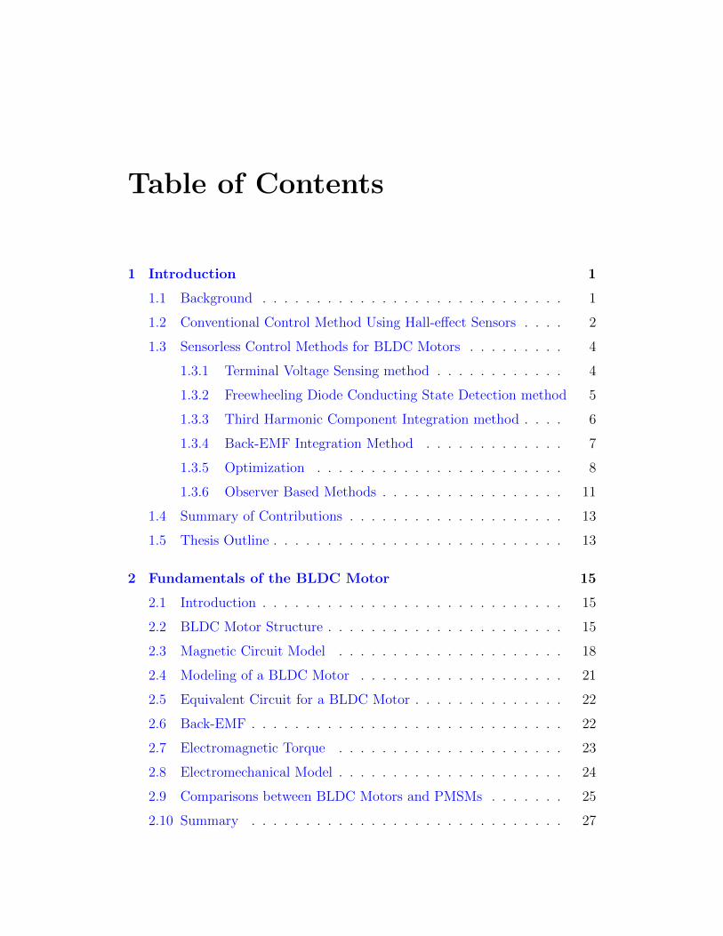
Table of Contents

1 Introduction 1

1.1 Background . . . . . . . . . . . . . . . . . . . . . . . . . . . . 1

1.2 Conventional Control Method Using Hall-effect Sensors . . . . 2

1.3 Sensorless Control Methods for BLDC Motors . . . . . . . . . 4

1.3.1 Terminal Voltage Sensing method . . . . . . . . . . . . 4

1.3.2 Freewheeling Diode Conducting State Detection method 5

1.3.3 Third Harmonic Component Integration method . . . . 6

1.3.4 Back-EMF Integration Method . . . . . . . . . . . . . 7

1.3.5 Optimization . . . . . . . . . . . . . . . . . . . . . . . 8

1.3.6 Observer Based Methods . . . . . . . . . . . . . . . . . 11

1.4 Summary of Contributions . . . . . . . . . . . . . . . . . . . . 13

1.5 Thesis Outline . . . . . . . . . . . . . . . . . . . . . . . . . . . 13

2 Fundamentals of the BLDC Motor 15

2.1 Introduction . . . . . . . . . . . . . . . . . . . . . . . . . . . . 15

2.2 BLDC Motor Structure . . . . . . . . . . . . . . . . . . . . . . 15

2.3 Magnetic Circuit Model . . . . . . . . . . . . . . . . . . . . . 18

2.4 Modeling of a BLDC Motor . . . . . . . . . . . . . . . . . . . 21

2.5 Equivalent Circuit for a BLDC Motor . . . . . . . . . . . . . . 22

2.6 Back-EMF . . . . . . . . . . . . . . . . . . . . . . . . . . . . . 22

2.7 Electromagnetic Torque . . . . . . . . . . . . . . . . . . . . . 23

2.8 Electromechanical Model . . . . . . . . . . . . . . . . . . . . . 24

2.9 Comparisons between BLDC Motors and PMSMs . . . . . . . 25

2.10 Summary . . . . . . . . . . . . . . . . . . . . . . . . . . . . . 27

3 Experimental Environment 28

3.1 Hardware Overview . . . . . . . . . . . . . . . . . . . . . . . . 28

3.2 Piccolo F28035 ISO controlCARD . . . . . . . . . . . . . . . . 30

3.2.1 ADC Module . . . . . . . . . . . . . . . . . . . . . . . 30

3.2.2 ePWM Module . . . . . . . . . . . . . . . . . . . . . . 30

3.3 DRV8312 Digital Motor Control Board . . . . . . . . . . . . . 31

3.3.1 DRV8312 . . . . . . . . . . . . . . . . . . . . . . . . . 31

3.3.2 Macro Blocks . . . . . . . . . . . . . . . . . . . . . . . 32

3.3.3 Power Domains of the Kit . . . . . . . . . . . . . . . . 34

3.3.4 PWMDAC Module . . . . . . . . . . . . . . . . . . . . 34

3.4 BLDC Motor . . . . . . . . . . . . . . . . . . . . . . . . . . . 35

3.5 Summary . . . . . . . . . . . . . . . . . . . . . . . . . . . . . 35

4 Sensorless BLDC Motor Drive Based on Line Voltage Differ-

ences 36

4.1 Six-step Commutation . . . . . . . . . . . . . . . . . . . . . . 36

4.1.1 Analysis of Six-step Commutation . . . . . . . . . . . . 36

4.2 Sensorless Commutation Method Based on Line Voltage Differ-

ences . . . . . . . . . . . . . . . . . . . . . . . . . . . . . . . . 40

4.3 Voltage Measurement . . . . . . . . . . . . . . . . . . . . . . . 44

4.4 Phase Delay Compensation . . . . . . . . . . . . . . . . . . . 45

4.5 Starting Procedure . . . . . . . . . . . . . . . . . . . . . . . 49

4.6 Electrical Noises . . . . . . . . . . . . . . . . . . . . . . . . . 49

4.7 Proposed Sensorless Drive . . . . . . . . . . . . . . . . . . . . 50

4.8 Experimental Results . . . . . . . . . . . . . . . . . . . . . . . 51

4.8.1 Experiment Results at 600 rpm . . . . . . . . . . . . . 51

4.8.2 Experiment Results at 1000 rpm . . . . . . . . . . . . 53

4.8.3 Phase Delay Compensation . . . . . . . . . . . . . . . 53

4.9 Summary . . . . . . . . . . . . . . . . . . . . . . . . . . . . . 57

5 Sensorless BLDC Motor Drive Based on Disturbance Observer 58

5.1 Disturbance Observer . . . . . . . . . . . . . . . . . . . . . . . 58

v

5.2 Sensorless Commutation Method Based on Disturbance Observer 60

5.3 Design of the Disturbance Observer . . . . . . . . . . . . . . . 63

5.4 Phase Delay Compensation . . . . . . . . . . . . . . . . . . . 66

5.5 Proposed Sensorless Drive . . . . . . . . . . . . . . . . . . . . 70

5.6 Experimental Results . . . . . . . . . . . . . . . . . . . . . . . 70

5.6.1 Experiment Results at 600 rpm . . . . . . . . . . . . . 71

5.6.2 Experiment Results at 1000 rpm . . . . . . . . . . . . 72

5.6.3 Phase Delay Compensation . . . . . . . . . . . . . . . 72

5.7 Comparison with the Sensorless Drive based on Line Voltage

Differences . . . . . . . . . . . . . . . . . . . . . . . . . . . . . 76

5.8 Summary . . . . . . . . . . . . . . . . . . . . . . . . . . . . . 77

6 Conclusions 79

6.1 Summary of Research . . . . . . . . . . . . . . . . . . . . . . . 79

6.2 Future Work . . . . . . . . . . . . . . . . . . . . . . . . . . . . 80

Bibliography 80

vi

List of Figures

1.1 World market growth for electric motors in automotive appli-

cations . . . . . . . . . . . . . . . . . . . . . . . . . . . . . . . 2

1.2 Hall-effect sensors outputs at 700 rpm . . . . . . . . . . . . . . 3

1.3 Third harmonic flux linkage . . . . . . . . . . . . . . . . . . . 7

1.4 Integrated areas of the back-EMF . . . . . . . . . . . . . . . . 8

1.5 Current flowing direction during PWM off time . . . . . . . . 10

2.1 Brushless DC motor waveforms . . . . . . . . . . . . . . . . . 16

2.2 Fundamental BLDC motor structure . . . . . . . . . . . . . . 17

2.3 A BLDC motor with the flux paths . . . . . . . . . . . . . . . 18

2.4 A magnetic circuit for BLDC motor . . . . . . . . . . . . . . . 19

2.5 Simplification of the magnetic circuit . . . . . . . . . . . . . . 20

2.6 Magnetic circuit considering the mutual coupling . . . . . . . 20

2.7 Equivalent circuit for BLDC motor . . . . . . . . . . . . . . . 22

3.1 Diagram of the DRV8312 Digital Motor Control Kit . . . . . . 29

3.2 DRV8312 Digital Motor Control (DMC) board . . . . . . . . . 29

3.3 Piccolo F28035 ISO controlCARD . . . . . . . . . . . . . . . . 30

3.4 Differential amplifier circuit on DRV8312 DMC board . . . . . 33

3.5 BLY172S-24V-4000 motor . . . . . . . . . . . . . . . . . . . . 35

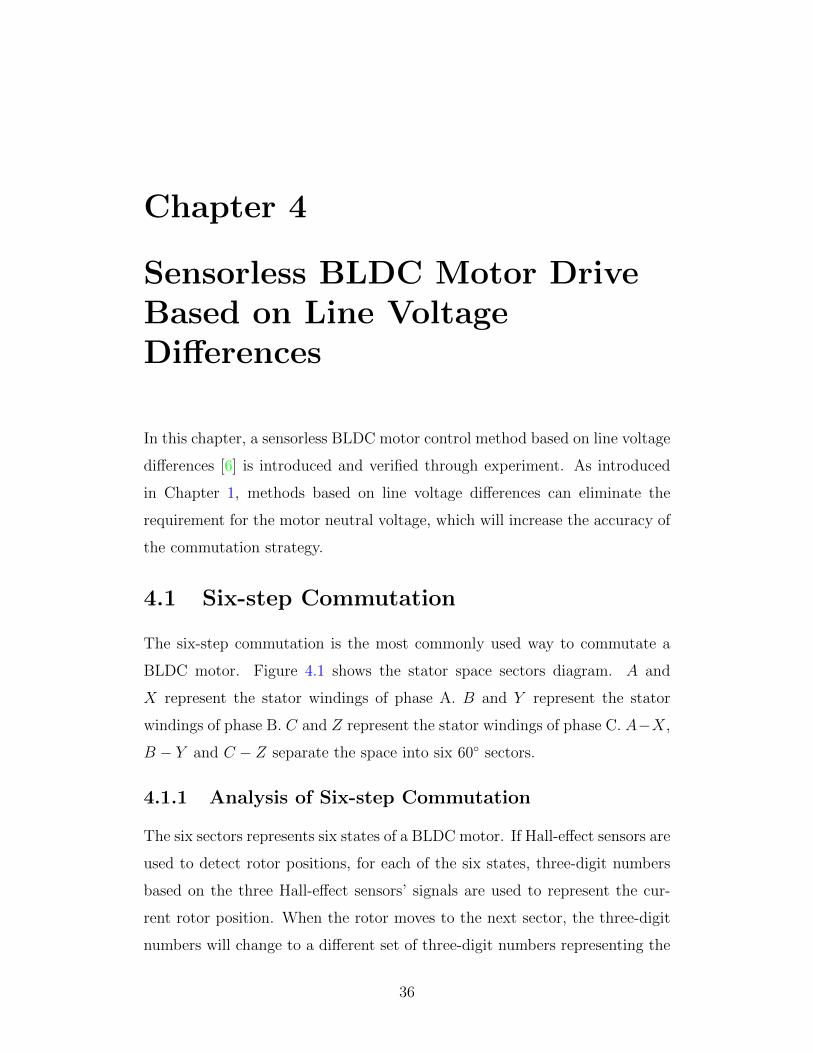
4.1 Stator space sectors diagram . . . . . . . . . . . . . . . . . . . 37

4.2 BLDC motor six-step commutation . . . . . . . . . . . . . . . 39

4.3 Simulation results of the line voltage differences and back-EMFs

waveforms . . . . . . . . . . . . . . . . . . . . . . . . . . . . . 43

4.4 Simulation results of the the combined commutation function . 44

4.5 Voltage resistor divider circuit . . . . . . . . . . . . . . . . . . 45

4.6 Software flowchart of the sensorless commutation method based

on line voltage differences . . . . . . . . . . . . . . . . . . . . 48

4.7 Proposed sensorless BLDC motor drive based on line voltage

differences . . . . . . . . . . . . . . . . . . . . . . . . . . . . . 51

4.8 Line voltage differences at 600 rpm . . . . . . . . . . . . . . . 52

4.9 Speed response at 600 rpm . . . . . . . . . . . . . . . . . . . . 52

4.10 Line voltage differences at 1000 rpm . . . . . . . . . . . . . . . 53

4.11 Speed response at 1000 rpm . . . . . . . . . . . . . . . . . . . 54

4.12 Phase A current and Vabca at 1800 rpm . . . . . . . . . . . . . 55

4.13 Speed response at 1800 rpm . . . . . . . . . . . . . . . . . . . 55

4.14 Commutation signals at 1800 rpm . . . . . . . . . . . . . . . . 56

5.1 Structure of DEF disturbance observer . . . . . . . . . . . . . 59

5.2 Simulation results of the back-EMF differences and phase currents 61

5.3 Applied disturbance observer structure . . . . . . . . . . . . . 62

5.4 Modified disturbance observer structure . . . . . . . . . . . . . 64

5.5 Estimated back-EMF differences at 1000 rpm . . . . . . . . . . 67

5.6 Estimated back-EMF differences at 2000 rpm . . . . . . . . . . 68

5.7 Software flowchart of the sensorless commutation method based

on the disturbance observer structure . . . . . . . . . . . . . . 69

5.8 Proposed sensorless BLDC motor drive based on the distur-

bance observer structure . . . . . . . . . . . . . . . . . . . . . 71

5.9 Estimated back-EMF differences at 600 rpm . . . . . . . . . . 71

5.10 Speed response at 600 rpm . . . . . . . . . . . . . . . . . . . . 72

5.11 Estimated back-EMF differences at 1000 rpm . . . . . . . . . . 73

5.12 Speed response at 1000 rpm . . . . . . . . . . . . . . . . . . . 73

5.13 Phase A current and eab at 1500 rpm . . . . . . . . . . . . . . 74

5.14 Speed response at 1500 rpm . . . . . . . . . . . . . . . . . . . 74

5.15 Commutation signals at 1500 rpm . . . . . . . . . . . . . . . . 75

5.16 Vabca at 300 rpm and eab at 250 rpm . . . . . . . . . . . . . . . 77

5.17 Speed response at 500 rpm during loading transient . . . . . . 78

viii

5.18 Speed response at 1500 rpm during loading transient . . . . . . 78

ix

List of Tables

1.1 Commutation function for the unknown input observer . . . . 12

2.1 Magnetic circuit model parameters . . . . . . . . . . . . . . . 19

3.1 BLDC motor specifications . . . . . . . . . . . . . . . . . . . . 35

4.1 Commutation states in six-step BLDC motor control . . . . . 38

4.2 Commutation sequence for the method based on line voltage

differences . . . . . . . . . . . . . . . . . . . . . . . . . . . . . 44

4.3 Terminal voltage sensing circuit specifications . . . . . . . . . 46

5.1 Commutation sequence for the method based on disturbance

observer . . . . . . . . . . . . . . . . . . . . . . . . . . . . . . 70

Chapter 1

Introduction

1.1 Background

In [30], it mentions that BLDC motors are better than induction motors and

brushed DC motors in many areas. Firstly, BLDC motors are smaller in size,

and have higher efficiency because of no losses in the rotor. Secondly, due to

the elimination of brushes, BLDC motors have better high speed capability,

and they do not need any brush maintenance. Thirdly, BLDC motors have a

faster response and a lower radio frequency interference (RFI). Also, BLDC

motors are designed with internal shaft position feedback, so that they have

higher starting torque compared with AC induction motors. Lastly, compared

to induction motors, BLDC motors have much better controllability because

of their linear speed torque characteristics.

The world market growth for electric motors in automotive applications

is shown in Figure 1.1, derived from the IMS research. As for global issues

like fuel shortage and global warming, the market for electric vehicles and

hybrid vehicles will continue to increase in the next few decades. With the

development of electrically-driven automotive systems, the demand for electric

motors is expected to grow, especially for BLDC motor shipments, which are

predicted to grow at twice the rate of other motor types.

BLDC motors have been applied in many other areas. For example, in the

Heating, ventilation and air conditioning (HVAC) and refrigeration industries,

BLDC motors have been applied to reduce the operating power requirements

instead of various types of AC motors. For medical applications, BLDC mo-

1

2012 2013 2014 2015 2016 20171

2

3

4

5

6

7

8

9

10

Year

Motor s

hipments

growth

(%)

StepperDC BrushedDC Brushless

Figure 1.1: World market growth for electric motors in automotive applications

tors, previously not an option, are now surging due to improvements in effi-

ciency and reliability. BLDC motors are also applied to industrial robots and

aerospace areas. BLDC motors are taking center stages and will be the future

trend, which will drive the growth in the BLDC motor market.

Since BLDC motors play a more and more important role in modern so-

ciety, it is of great value for us to research on BLDC motor drive systems to

make them better for applications in various areas.

1.2 Conventional Control Method Using Hall-

effect Sensors

BLDC motors need rotor positions for proper commutation of stator currents.

For a permanent magnet AC synchronous (PMAC) motor, a resolver or a shaft

encoder is normally applied to detect rotor positions because constant infor-

mation of rotor positions is required for PMAC motor control [8]. However, for

a BLDC motor, one electrical cycle contains only six commutation instants,

2

0.6 0.61 0.62 0.63 0.64 0.65 0.66−1

0

1

2

time (s)

HallA

0.6 0.61 0.62 0.63 0.64 0.65 0.66−1

0

1

2

time (s)

HallB

0.6 0.61 0.62 0.63 0.64 0.65 0.66−1

0

1

2

time (s)

HallC

Figure 1.2: Hall-effect sensors outputs at 700 rpm

so Hall-effect sensors are often used, which can reduce the costs [19].

BLDC motors are controlled electronically instead of using mechanical

commutation. Hall-effect sensors can be mounted in one of three locations

inside the motor to measure the motor’s positions. When permanent mag-

netic north or south poles pass near the Hall-effect sensors, the Hall-effect

sensors will generate low or high signals accordingly. Figure 1.2 shows a simu-

lation result of the outputs of Hall-effect sensors at a speed of 700 rpm. Based

on the output signals sent from three Hall-effect sensors, the current state can

be determined and currents will be applied to corresponding motor coils.

However, the control method based on hall sensors has some drawbacks.

High temperature will affect the performance of hall sensors thereby limiting

their application areas. The cost and weight of motors will also increase and

extra mechanical arrangement need to be mounted [6]. To increase system

reliability and reduce system cost, sensorless control of BLDC motors has

attracted wide attentions.

3

1.3 Sensorless Control Methods for BLDC Mo-

tors

If a PM motor drive only needs electrical measurements without any require-

ments for a position sensor, it is called a sensorless drive [2]. There are many

kinds of sensorless drives for BLDC motors. Among them, back electromotive

force (back-EMF) based methods are the most commonly used category.

Conventional back-EMF based methods utilize the terminal voltage in the

floating phase [20][19][13], detection of the conducting state of freewheeling

diode in the floating phase [31][6], third harmonic components of back-EMF

waveforms [9] and integration of the floating phase back-EMF [1].

However, back-EMFs values are zero at standstill, and it is difficult to

detect the zero-crossing points from noises if the motor speed is low, so the

low speed performance is limited. For methods based on back-EMFs, a starting

procedure is normally required to speed up BLDC motors to a relatively higher

speed, and then motors can be controlled by sensorless drives [8].

1.3.1 Terminal Voltage Sensing method

The terminal voltage sensing method is one of the common methods among

back-EMFs based sensorless techniques.

For the trapezoidal control of BLDC motors, back-EMFs are required to

be in phase with the phase currents, so the motor is able to produce a constant

torque [8]. The most commonly way is to detect the zero-crossing points of the

back-EMF in the floating phase [22]. There is a 30 offset between zero-crossing

points of back-EMFs and current commutation instants, so a 30 phase shift

needs to be applied to get the correct commutation instances [20].

Since the back-EMFs are determined with respect to the motor neutral

point, the neutral point voltage must be compare with terminal voltages to

get the zero-crossing points of back-EMFs. However, neutral points are not

available in most BLDC motors. The most commonly used approach is to

connect the terminals of the BLDC motor to a Y-connected resistive network.

The virtual neutral point voltage can be used to compare with the terminal

4

voltage in the floating phase to get the zero-crossing points.

However, the virtual neutral point voltage contains lots of electrical noises

because the pulse width modulation (PWM) technique is normally applied to

drive the inverter. Another approach is to compare terminal voltages with half

of the DC link voltage to get back-EMFs zero-crossing points [19]. Work in

[28] mentioned that the measurements do not contain any noises if sampling

during PWM on time.

Low pass filters are normally applied to attenuate the high frequency har-

monics components in terminal voltages introduced by PWM. However, low

pass filters will cause a time delay which becomes more obvious when a BLDC

motor runs at high speeds range. With no phase compensation, the time delay

will restrict the suitable high speed range of BLDC motors. Because the back-

EMF magnitude is in proportion to the motor speed, it is unable to detect

back-EMFs at standstill and low speed, which is another drawback of termi-

nal voltage sensing method [8]. Therefore, conventional open-loop starting

method will be applied to speed up a BLDC motor from standstill.

1.3.2 Freewheeling Diode Conducting State Detectionmethod

Work in [31] proposed an method which can estimate the commutation points

on the basis of the conducting state of the freewheeling diode which is in paral-

lel with the power transistor in the floating phase. Six commutation instants

for one electrical cycle can be obtained based on whether the freewheeling

diode is conducting or not. This detected point leads the next commutation

instant by 30 degrees, so a phase shift is required. The conducting condition

of the freewheeling diode at the negative side of phase C is derived as:

ec < −V1 + V2

2(1.1)

where V1 is the transistors voltage drop, V2 is the diodes voltage drop and ec

is the back-EMF of phase C. Compared with the back-EMF value, V1 and V2

are negligible. When ec changes from positive to negative, the current flowing

through the freewheeling diode at the negative side of phase C will be detected

5

as.

Because the conducting of the freewheeling diodes relies on back-EMFs

value, detection of the rotor position at low speeds is hard to realize, so a

starting process is applied [8]. The main drawback of this method is that for

detection of current flowing in each freewheeling diode, a separate power supply

for the comparator circuit is required [6]. These additional requirements will

limit this method in real applications.

1.3.3 Third Harmonic Component Integration method

Works in [29] mentioned that the third harmonic component of back-EMF

waveforms are applied to estimate the commutation points. The trapezoidal

waveforms of the BLDC motor back-EMFs consist of fundamental and higher

order harmonics. After summing the three terminal voltages, the third har-

monic component of back-EMF waveforms is obtained [20]:

Vresult = Van + Vbn + Vcn

=

(R + L

d

dt

)(ia + ib + ic) + ea + eb + ec

= ea + eb + ec ≈ 3e3sin (3θr)

(1.2)

where Vresult is the summation result of the three terminal voltages, Van, Vbn

and Vcn are the phase voltages with respect to the motor neutral voltage, R

is the phase stator resistance, L is the phase stator inductance, ea, eb and ec

are the phase back-EMFs, ia, ib and ic are the phase currents, e3 is the third

harmonic component of back-EMF waveforms and θr is the electrical angle.

Because during each state, the sum of three phase currents (ia + ib + ic)

is equal to zero. Vresult is dominated by the third harmonic component and

contains only third-order harmonics (3rd, 6th, 9th). After integrating Vresult,

the third harmonic flux linkage can be obtained as:

λ =

∫Vresultdt (1.3)

where λ is the third harmonic flux linkage [8].

Based on the results in [29], the zero-crossing points of λ are identical to

the current commutation points as shown in Figure 1.3. The main advantage

6

of this technique is that Vresult does not contain the switching noises caused by

PWM signals. In comparison with other sensorless control methods which need

a low pass filter, this method requires less filtering [20]. Due to insensitivity to

filtering delay, this method can work over a wider speed range. Theoretically,

this sensorless commutation method is suitable for a wide speed range and it

can work at various load conditions. Its performance at lower speeds is also

better because third harmonics can be detected even when the speed is low.

λ

θ (degree)

θ (degree)60 120 180 240 300

Commutation

360 420 4800

Signal

Figure 1.3: Comparison of the zero-crossing points of λ and the commutationsignal

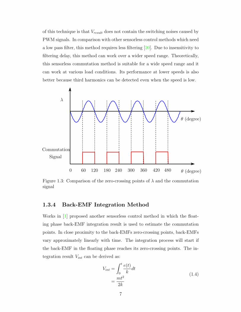
1.3.4 Back-EMF Integration Method

Works in [1] proposed another sensorless control method in which the float-

ing phase back-EMF integration result is used to estimate the commutation

points. In close proximity to the back-EMFs zero-crossing points, back-EMFs

vary approximately linearly with time. The integration process will start if

the back-EMF in the floating phase reaches its zero-crossing points. The in-

tegration result Vint can be derived as:

Vint =

∫ t

0

e(t)

kdt

=mt2

2k

(1.4)

7

where k is the integration gain, t is the integration end time, e(t) is the back-

EMF value and m is the slope of the back-EMF waveform.

The integration process will stop when Vint reaches the predefined thresh-

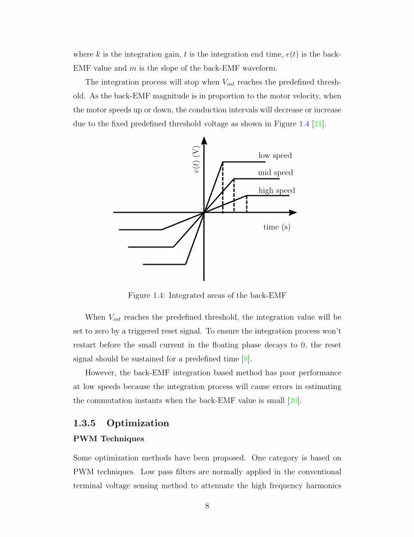
old. As the back-EMF magnitude is in proportion to the motor velocity, when

the motor speeds up or down, the conduction intervals will decrease or increase

due to the fixed predefined threshold voltage as shown in Figure 1.4 [21].

time (s)

e(t)

(V)

high speed

mid speed

low speed

Figure 1.4: Integrated areas of the back-EMF

When Vint reaches the predefined threshold, the integration value will be

set to zero by a triggered reset signal. To ensure the integration process won’t

restart before the small current in the floating phase decays to 0, the reset

signal should be sustained for a predefined time [8].

However, the back-EMF integration based method has poor performance

at low speeds because the integration process will cause errors in estimating

the commutation instants when the back-EMF value is small [20].

1.3.5 Optimization

PWM Techniques

Some optimization methods have been proposed. One category is based on

PWM techniques. Low pass filters are normally applied in the conventional

terminal voltage sensing method to attenuate the high frequency harmonics

8

components in terminal voltages introduced by PWM. The low pass filter

will cause time delay which limits high speed performance, if no phase delay

compensation method is applied. However, PWM strategies can eliminate the

requirements for low pass filters and work well over a wide speed range [24].

For conventional PWM methods, one upper transistor in one phase and

one lower transistor in another phase are conducting at the same time. The

remaining phase is the floating phase [31].This approach will increase power

losses in the motor side because of the high harmonic components [25].

Work in [36] proposed a direct back-EMF detection method based on the

PWM strategy. The direct back-EMF detection method eliminates the need

for virtual neutral voltage. In this method, PWM only applies to upper tran-

sistors, and lower transistors will be left on. Considering the condition that

phase A and B are conducting current, PWM is applied to the upper transistor

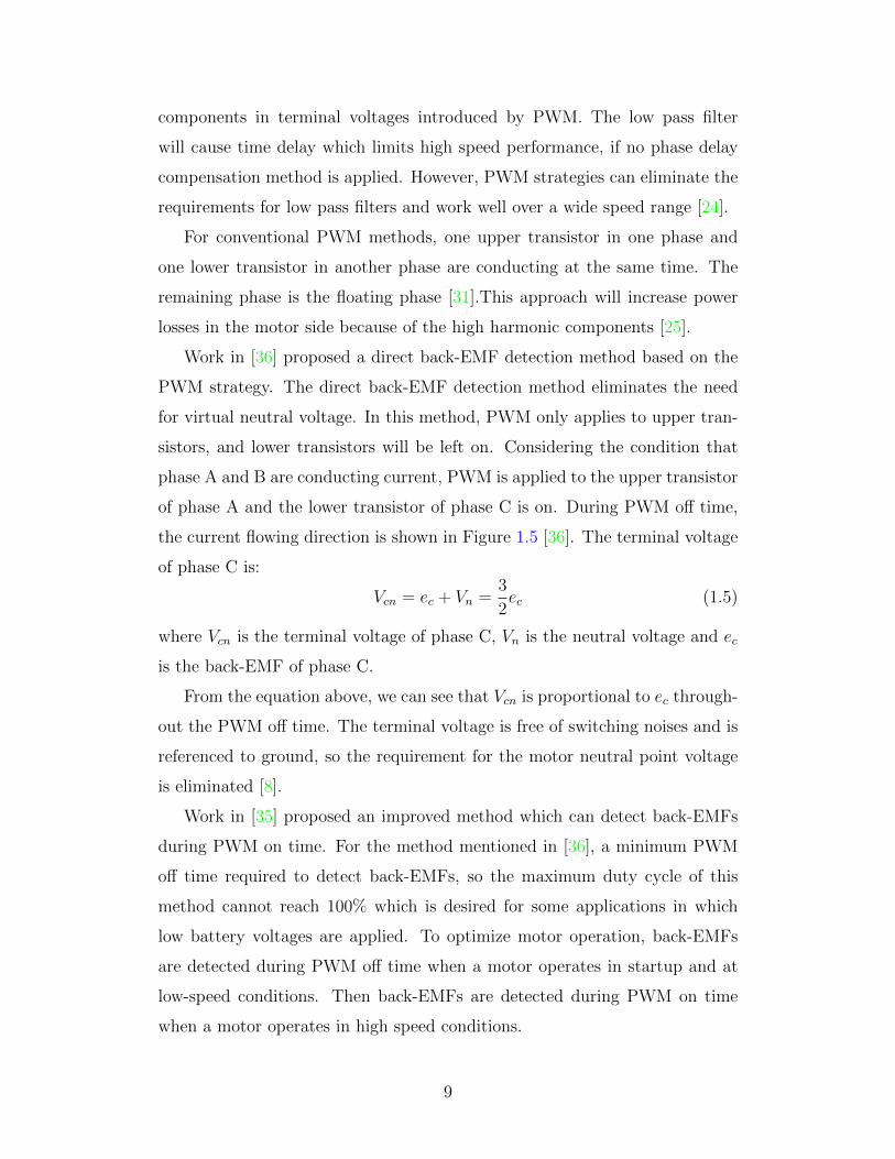
of phase A and the lower transistor of phase C is on. During PWM off time,

the current flowing direction is shown in Figure 1.5 [36]. The terminal voltage

of phase C is:

Vcn = ec + Vn =3

2ec (1.5)

where Vcn is the terminal voltage of phase C, Vn is the neutral voltage and ec

is the back-EMF of phase C.

From the equation above, we can see that Vcn is proportional to ec through-

out the PWM off time. The terminal voltage is free of switching noises and is

referenced to ground, so the requirement for the motor neutral point voltage

is eliminated [8].

Work in [35] proposed an improved method which can detect back-EMFs

during PWM on time. For the method mentioned in [36], a minimum PWM

off time required to detect back-EMFs, so the maximum duty cycle of this

method cannot reach 100% which is desired for some applications in which

low battery voltages are applied. To optimize motor operation, back-EMFs

are detected during PWM off time when a motor operates in startup and at

low-speed conditions. Then back-EMFs are detected during PWM on time

when a motor operates in high speed conditions.

9

ea

eb

ec

R

R

R

L

L

L

Va

Vb

Vc

Vn

i

VDC

GND

Figure 1.5: Current flowing direction during PWM off time

Lai, Yen-Shin, and Yong-Kai Lin proposed a similar method to detect

zero-crossing points of back-EMF waveforms. For PWM on and off states,

different methods are applied to detect zero-crossing points, and this sensorless

commutation method can work over a wide speed range [24]. The difference

between these two methods is that the second one uses a digital controller to

calculate zero-crossing points instead of using logical comparisons.

Methods Based on Terminal Line to Line Voltages

Another category is based on terminal line to line voltages rather than using

the terminal voltage in the floating phase. In this category, the requirement

for the motor neutral voltage can be eliminated.

Based on the work in [4], we can directly get the commutation instants

from the average terminal line to line voltages of BLDC motors. The average

line to line voltages are in phase with the Hall-effect sensors, so that can be

used directly without the need of a phase shift. Also, it does not need the

motor neutral voltage compared with the conventional method.

10

Line voltage differences can also be applied to estimate back-EMF zero-

crossing points. Line voltage differences have the same zero-crossing points

as the back-EMFs [6]. As line voltages are applied, we can eliminate the

requirement for the motor neutral voltage.

The commutation points of BLDC motor currents are identical to the zero-

crossing points of line to line back-EMFs, so line to line back-EMFs are applied

directly to estimate BLDC motor commutation points without any phase shifts

[39]. Work in [26] proposed a novel commutation function based on calculated

line to line back-EMFs to estimate commutation instants. Commutation in-

stants occur when the commutation function changes from positive infinity to

negative infinity or from negative infinity to positive infinity. Work in [19]

proposed a method which uses a circuit constituting a differential amplifier

and a comparator to detect zero-crossing points of line to line back-EMFs.

1.3.6 Observer Based Methods

For PMAC motors, observer based methods are often used because they have

sinusoidal back-EMFs, and continuous rotor positions information is required

[8]. Different observers have also been applied to estimate the rotor positions

of BLDC motors.

Observer based methods often take measurements as inputs of the mathe-

matical model of BLDC motors, and take the output as the estimated results.

The difference between the measurements and the estimated results is sent

back to the mathematical model to make a correction.

The Extended Kalman Filter (EKF) can be employed to estimate rotor

positions and motor speed by using average line voltages and the measured

phase currents [37]. With the predictive current controller, average line volt-

ages are calculated at the beginning of the sampling interval. However, EKF

cannot obtain satisfactory estimation results when the motor speed is low.

Based on the work in [11], the computation burdens and difficulties to tuning

the control systems are significant drawbacks of EKF based methods, and the

sliding mode observer is an attractive method because it is robust despite the

measurement noises and parametric uncertainty of the system.

11

Sliding mode observer is designed based on dynamic equations of BLDC

motors to estimate back-EMF values, rotor positions and the motor speed. For

conventional methods, a fixed sliding mode observer gain is used to estimate

back-EMF values which only suits a particular range of speed. The fixed

observer gain will produce multiple zero-crossings when the motor speed is

low. Also, it will cause a phase delay in many cases. An improvement has

been made to modify the observer gains according to the motor speed, so the

estimated back-EMF values are more accurate [7].

Back-EMF differences signals can also be estimated by observers. Work

in [22] proposed a new sensorless control method which utilizes an unknown

input observer. The unknown input observer is independent of the rotor speed

and can be used to estimate back-EMF differences. As shown in table 1.1, the

estimated back-EMF differences are used in the commutation functions to get

commutation instants.

Electrical Degree Commutation Function

0-60 ebc/eca60-120 eab/ebc120-180 eca/eab180-240 ebc/eca240-300 eab/ebc300-360 eca/eab

Table 1.1: Commutation function for the unknown input observer

For methods above, continuous rotor positions information is estimated.

However, for trapezoidal control of BLDC motors, only 6 commutation points

are needed for one electrical cycle, so the complex observer based methods

above are not necessary for the control of BLDC motors. Disturbance ob-

server structure can be used to estimate the back-EMF differences signals

[39]. This method is easier to implement, and it can precisely estimate the six

commutation instants.

12

1.4 Summary of Contributions

This thesis implements and verifies two sensorless control methods based on

line voltage differences and the disturbance observer respectively. Instead of

sampling terminal voltages during PWM on time to avoid noises [6], this the-

sis uses a simpler method in which low pass filters are applied to filter out

the high frequency harmonics components introduced by PWM. Compensa-

tion methods are included in the sensorless drives to compensate the phase

delay introduced by the low pass filters, which will guarantee the high speeds

operation of the BLDC motors. Also, the robustness of the sensorless control

methods during loading transient is demonstrated by simulation results.

1.5 Thesis Outline

Chapter 2 makes a detailed analysis of the fundamentals of BLDC motors.

Firstly, it provides an introduction to the BLDC motor structure with empha-

sis on the stator and rotor. Chapter 2 also presents the equivalent circuit and

the mathematical model of a BLDC motor, which are applied in the derivations

of Chapter 4 and Chapter 5. Back-EMF, which is the basis of the sensorless

control methods applied in this thesis, is analyzed. Finally, a comparison is

made between BLDC motors and PMSMs with respect to power density, power

losses, control complexity, and torque ripples.

Chapter 3 outlines the experimental environment of this thesis. The DRV8312

Digital Motor Control Kit, in essence a Piccolo F28035 controlCARD, a DRV8312

Digital Motor Control board and a BLDC motor, on which all the experiment

work is based, is introduced and discussed.

Chapter 4 presents a six-step sensorless control method based on the line

voltage differences. The Simulink simulation results verify that the line voltage

differences have the same zero-crossing points as the back-EMFs. In order to

get the six commutation instants for one electrical cycle of the BLDC motor,

a phase delay compensation method is applied in consideration of the time

delay caused by low pass filters. This sensorless drive is implemented in the

13

experimental environment under different speed conditions.

Chapter 5 introduces another six-step sensorless control method based on

the disturbance observer. The disturbance observer is applied to estimate

back-EMF differences. The Simulink simulation results show that the zero-

crossing points of the back-EMF differences are identical to the BLDC motor

commutation instants. A different phase delay compensation method is ap-

plied to compensate for the time delay caused by the disturbance observer

structure. The sensorless control method is further verified in the experimen-

tal environment. Finally, we make a comparison of these two sensorless drives.

Chapter 6 summarizes the thesis and makes discussions on possible future

research directions.

14

Chapter 2

Fundamentals of the BLDCMotor

2.1 Introduction

In this chapter, we will make an introduction to the fundamentals of the

BLDC motor mainly based on the theories in these three references [10][23][40].

Based on the back-EMF waveform shapes, (i.e., sinusoidal and trapezoidal),

the permanent magnet synchronous machines can be classified into two differ-

ent types. The trapezoidal type is called the BLDC motor and the sinusoidal

type named the PMSM.

Figure 2.1 [23] shows waveforms of BLDC motors. For one electrical cycle

of a BLDC motor, it contains six states. During each state, two phases are

conducting and each phase will be excited for 120. The induced back-EMFs

are in the trapezoidal shape, and the constant magnitude remains for 120.

During the change states (from maximum to minimum, or from minimum to

maximum), the induced back-EMFs vary linearly.

2.2 BLDC Motor Structure

Figure 2.2 [12] shows the fundamental structure of a BLDC motor. A BLDC

motor contains a rotating part, called the rotor, and a stationary frame, called

the stator. In this example, the rotor has two pairs of north and south per-

manent magnet poles. The stator acts as the armature because it will be

energized, and the stator current will generate the rotating magnetic field. As

15

θr (degree)

30 150

270

330

90

ea

eb

ec

ia

ib

ic

Te

210

Figure 2.1: Brushless DC motor waveforms

16

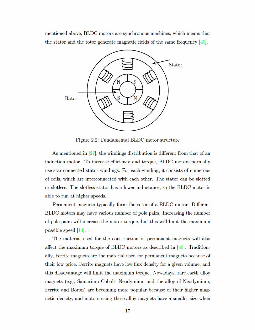
mentionedabove,BLDCmotorsaresynchronousmachines,whichmeansthat

thestatorandtherotorgeneratemagneticfieldsofthesamefrequency[40].

N

S N

S

Stator

Rotor

Figure2.2:FundamentalBLDCmotorstructure

Asmentionedin[27],thewindingsdistributionisdifferentfromthatofan

inductionmotor. Toincreaseefficiencyandtorque,BLDCmotorsnormally

usestarconnectedstatorwindings.Foreachwinding,itconsistsofnumerous

ofcoils,whichareinterconnectedwitheachother.Thestatorcanbeslotted

orslotless.Theslotlessstatorhasalowerinductance,sotheBLDCmotoris

abletorunathigherspeeds.

PermanentmagnetstypicallyformtherotorofaBLDCmotor.Different

BLDCmotorsmayhavevariousnumberofpolepairs.Increasingthenumber

ofpolepairswillincreasethemotortorque,butthiswilllimitthemaximum

possiblespeed[14].

Thematerialusedfortheconstructionofpermanentmagnetswillalso

affectthemaximumtorqueofBLDCmotorsasdescribedin[40].Tradition-

ally,Ferritemagnetsarethematerialusedforpermanentmagnetsbecauseof

theirlowprice.Ferritemagnetshavelowfluxdensityforagivenvolume,and

thisdisadvantagewilllimitthemaximumtorque.Nowadays,rareearthalloy

magnets(e.g.,SamariumCobalt,NeodymiumandthealloyofNeodymium,

FerriteandBoron)arebecomingmorepopularbecauseoftheirhighermag-

neticdensity,andmotorsusingthesealloymagnetshaveasmallersizewhen

17

comparingwithmotorsofsameweightusingferritemagnets.

Stator

Rotor

S

S

N

N

Figure2.3:ABLDCmotorwiththefluxpaths

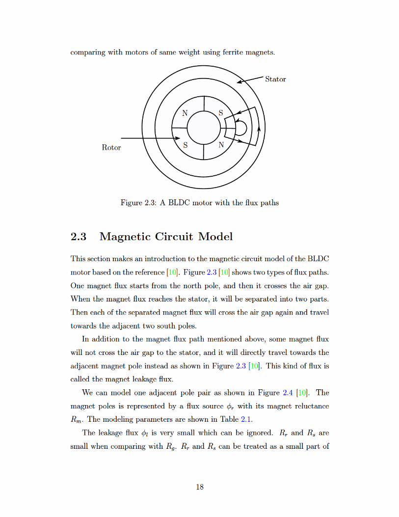
2.3 MagneticCircuit Model

ThissectionmakesanintroductiontothemagneticcircuitmodeloftheBLDC

motorbasedonthereference[10].Figure2.3[10]showstwotypesoffluxpaths.

Onemagnetfluxstartsfromthenorthpole,andthenitcrossestheairgap.

Whenthemagnetfluxreachesthestator,itwillbeseparatedintotwoparts.

Theneachoftheseparatedmagnetfluxwillcrosstheairgapagainandtravel

towardstheadjacenttwosouthpoles.

Inadditiontothemagnetfluxpathmentionedabove,somemagnetflux

willnotcrosstheairgaptothestator,anditwilldirectlytraveltowardsthe

adjacentmagnetpoleinsteadasshowninFigure2.3[10].Thiskindoffluxis

calledthemagnetleakageflux.

WecanmodeloneadjacentpolepairasshowninFigure 2.4[10]. The

magnetpolesisrepresentedbyafluxsourceφrwithitsmagnetreluctance

Rm.ThemodelingparametersareshowninTable2.1.

Theleakagefluxφlisverysmallwhichcanbeignored.RrandRsare

smallwhencomparingwithRg.RrandRscanbetreatedasasmallpartof

18

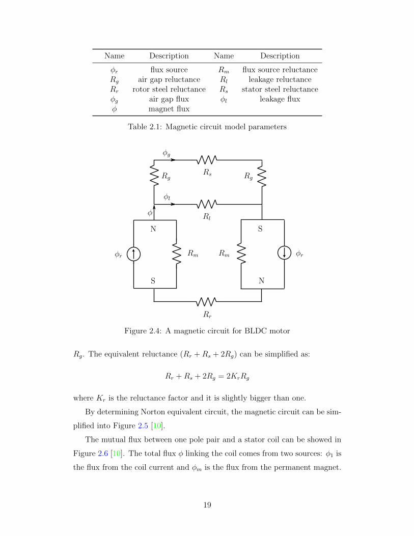
Name Description Name Description

φr flux source Rm flux source reluctanceRg air gap reluctance Rl leakage reluctanceRr rotor steel reluctance Rs stator steel reluctanceφg air gap flux φl leakage fluxφ magnet flux

Table 2.1: Magnetic circuit model parameters

Rmφr

N

S

Rm φr

S

N

Rr

Rs

Rl

Rg Rg

φg

φl

φ

Figure 2.4: A magnetic circuit for BLDC motor

Rg. The equivalent reluctance (Rr +Rs + 2Rg) can be simplified as:

Rr +Rs + 2Rg = 2KrRg

where Kr is the reluctance factor and it is slightly bigger than one.

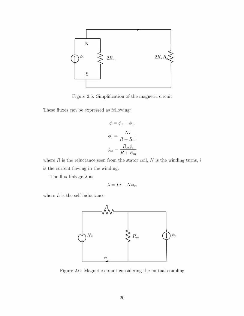
By determining Norton equivalent circuit, the magnetic circuit can be sim-

plified into Figure 2.5 [10].

The mutual flux between one pole pair and a stator coil can be showed in

Figure 2.6 [10]. The total flux φ linking the coil comes from two sources: φ1 is

the flux from the coil current and φm is the flux from the permanent magnet.

19

N

S

2Rm2KrRgφr

Figure 2.5: Simplification of the magnetic circuit

These fluxes can be expressed as following:

φ = φ1 + φm

φ1 =Ni

R +Rm

φm =Rmφr

R +Rm

where R is the reluctance seen from the stator coil, N is the winding turns, i

is the current flowing in the winding.

The flux linkage λ is:

λ = Li+Nφm

where L is the self inductance.

Rm

R

φrNi

φ

Figure 2.6: Magnetic circuit considering the mutual coupling

20

2.4 Modeling of a BLDC Motor

The BLDC motor modeling is based on the reference [23]. For the three stator

windings of a BLDC motor, the electrical relationships can be represented with

the equation below:VanVbnVcn

=

R 0 00 R 00 0 R

iaibic

+d

dt

Laa Lab Lac

Lba Lbb Lbc

Lca Lcb Lcc

iaibic

+

eaebec

(2.1)

where Van, Vbn and Vcn are the phase voltages referenced to the motor neutral

voltage, ia, ib and ic are the phase currents, ea, eb and ec are the phase back-

EMFs, R is the phase stator resistance which is same for three phases, Laa,

Lbb and Lcc are the self-inductances, Lab, Lba, Lac, Lca, Lbc and Lcb are the

mutual inductances.

If three phases are symmetric and the rotor reluctance is identical with

the change of electrical angle, the three self-inductances are same and the six

mutual inductances are equal to each other as:

Laa = Lbb = Lcc = Ls (2.2)

Lab = Lba = Lac = Lca = Lbc = Lcb = M (2.3)

The equivalent inductance L can be calculated as:

L = Ls −M (2.4)

Assuming that the phase currents are symmetric, that is

ia + ib + ic = 0 (2.5)

Then the electrical relationships can be simplified and the BLDC motor can

be modeled as:VanVbnVcn

= R

1 0 00 1 00 0 1

iaibic

+d

dt

L 0 00 L 00 0 L

iaibic

+

eaebec

(2.6)

21

2.5 Equivalent Circuit for a BLDC Motor

For a three-phase BLDC motor, the electrical circuit model can be shown

in Figure 2.7. In this circuit, R represents the resistance component of the

stator winding and L represents the inductive component of the stator phase

winding.

R

Leb

R

L

ea

ecL

R+

+

+

a

bc

n

Figure 2.7: Equivalent circuit for BLDC motor

ea, eb and ec are the phase back-EMFs. Because the resistance and in-

ductance are very small for the BLDC motor, the phase currents need to be

limited during starting up. Normally, PWM technique is applied for BLDC

motor control, and a small duty cycle is set during starting up.

2.6 Back-EMF

This section introduces the back-EMF of a BLDC motor based on the reference

[23]. When starting the BLDC motor, stator coils will be energized and a

torque will be generated on the rotor. Then the rotor will begin to rotate

and the flux linkage in the stator coils will vary depending on permanent

magnets locations. According to Faraday’s law of induction, a voltage will

be induced across the stator windings due to the varying flux linkage. This

induced voltage is referenced to back-EMF. The polarity of voltage induced is

22

governed by Lenz’s law. That is, the back-EMF will always try to keep the

flux linkage from changing its present value.

For BLDC motors, the back-EMFs are in trapezoidal shape. The peak

value of the back-EMFs is Ep which can be calculated as:

Ep = Keω (2.7)

where ω is the mechanical speed of the motor in rad/s, Ke is back-EMF con-

stant and its unit is V/(rad/s).

Ke can be calculated as:

Ke = NBlr (2.8)

where B is the flux density, N represents the conductors number per phase, l

is the conductor length, r is the air gap radius between the motor rotor and

stator.

From the equations above, the peak value of the back-EMFs depends

mainly on ω, B and N . Once the motor is designed, the back-EMF con-

stant Ke remains the same. The peak value of the back-EMFs is proportional

to the mechanical speed of the rotor.

The instantaneous back-EMFs can be written as:

ea = fa (θr)Keω (2.9)

eb = fb (θr)Keω (2.10)

ec = fc (θr)Keω (2.11)

where θr is the electrical degree, fa, fb and fc are in the trapezoidal shape as

the back-EMFs, and their peak magnitude is 1.

2.7 Electromagnetic Torque

From the energy conversion point, a BLDC motor converts electrical power to

mechanical power to make the motor rotate. Each phase of a BLDC motor is

composed of a resistive component and an inductive component [23].

The stator current flowing through the winding will create ohmic losses

or heat in the winding resistor. The current will also create a magnetic field

23

that stores energy. When phase currents flow through back-EMF sources, the

instantaneous power Pinstant absorbed by sources can be derived as:

Pinstant = eaia + ebib + ecic (2.12)

To satisfy the conservation of energy, this power will be converted to me-

chanical power Teω. The electromagnetic torque is given by:

Te = [eaia + ebib + ecic]1

ω(2.13)

Because back-EMFs are proportional to speed, the electromagnetic torque

can be derived as [23]:

Te = Kt [fa (θr) ia + fb (θr) ib + fc (θr) ic]

= Kt(2Ipd)(2.14)

where Ipd is the peak value of the phase current, Kt is the torque constant and

its units are Nm/A. Once the motor is designed, Kt is a constant. As a result,

the electromagnetic torque is directly proportional to the stator currents of a

BLDC motor.

Ke and Kt are numerically equal. The units for back-EMF constant Ke

and the torque constant Kt are equivalent if they are all in SI units as shown

in the equation below:

Nm/A = V/(rad/s) = kg ·m2/A · s2 (2.15)

2.8 Electromechanical Model

For BLDC motors, the absorbed instantaneous power of back-EMF sources

will be converted to mechanical power Teω.

The electromagnetic torque is used to drive the motor rotor to rotate. As-

suming that the system inertia is J , friction coefficient isB, and the load torque

is T1 if the BLDC motor drives a load, the equation for the electromechanical

model of the BLDC motor can be shown as [23]:

Jdω

dt+Bω = (Te − T1) (2.16)

24

and the relationship between the motor synchronous speed and the rotor po-

sition can be expressed as:dθrdt

=p

2ω (2.17)

where p is the rotor poles number, ω is the mechanical speed of the motor in

rad/s, θr is the rotor position in rad.

At the moment a BLDC motor starts, there is no back-EMF, and the

stator current will produce maximum electromagnetic torque on the motor

rotor. The motor will speed up, and the peak values of back-EMFs will also

increase proportionally. During this process, the stator currents will decrease,

and the motor speed will become stable finally.

2.9 Comparisons between BLDC Motors and

PMSMs

In this section, some comparisons will be made between BLDC motors and

PMSMs on their output power and torque ripples based on the reference [23].

The rms values of the stator currents are:

Im =Ipm√

2(2.18)

Id =

√2

3Ipd (2.19)

where Ipm and Ipd are the peak values of the stator currents in PMSMs and

BLDC motors, respectively. Im is the rms value of the stator current in

PMSMs, and Id is the rms value of the stator current in BLDC motors.

From the equations above, we can see that BLDC motors have a smaller

rms value than that of the sinusoidal PMSMs if their stator currents have the

same peak value. Assuming that PMSMs and BLDC motors have the same

ohmic losses, the relationship can be derived as:

3I2mR = 3I2dR (2.20)

where R is the phase stator resistance which is the same for all three phases.

25

Based on the analysis above, the relationship between the peak value of

PMSMs and BLDC motors currents can be derived as:

Ipd =

√3

2Ipm (2.21)

From the current waveforms of a BLDC motor, we can see that only two of

the three phases are conducting at the same time. Consequently, the output

power of a BLDC motor is contributed by only two phases. For a PMSM, all

three phases have currents and contribute to output power. Assuming that

PMSMs and BLDC motors back-EMFs have the same peak value Ep, the ratio

of a BLDC motor and a PMSM output power can be calculated as:

Power output radio =BLDC motor power

PMSM motor power(2.22)

=2× Ep × Ipd3× Ep√

2× Ipm√

2

= 1.1547 (2.23)

Based on the analysis above, If PMSMs and BLDC motors have same

ohmic losses, the output power of BLDC motors will be 15.4 % higher than

that of PMSMs. For BLDC motors, only two phases are conducting currents

at the same time, so the duty cycle of the phase currents is smaller than that

of PMSMs. The power losses are smaller in BLDC motors, and the inverter

thermal reliability is also better. Although, the currents of BLDC motors

and PMSMs both have variable frequencies, the rectangular phase currents of

BLDC motors have lower control complexity compared with PMSMs.

The torque ripples of BLDC motors are higher than PMSMs. During the

finite current transition time, torque ripples are created at each commutation

point. Torque ripples will be created whenever currents or back-EMF wave-

forms are not ideal. For low-performance applications, the torque ripples are

rarely significant. However, torque ripples are hard to eliminate and this will

limit the use of BLDC motors in applications where minimum torque ripples

are required. Knowing how to minimize torque ripples is very important for

high-performance applications.

26

2.10 Summary

In this chapter, we make an introduction to the BLDC motor structure, the

magnetic circuit model and the electrical model of a BLDC motor. Back-EMF

and electromagnetic toque concepts are also introduced. Finally a comparison

is made between PMSMs and BLDC motors. BLDC motors have a higher

output power but with larger torque ripples.

27

Chapter 3

Experimental Environment

In this thesis, all the experiment work is based on the DRV8312-C2 kit, which

is developed by Texas Instruments. This kit is a Medium Voltage Digital

Motor Control (DMC) kit. In this chapter, an introduction will be made to

the hardware details and the development environment.

3.1 Hardware Overview

The DRV8312 Digital Motor Control Kit includes a Piccolo F28035 control-

CARD, a DRV8312 Digital Motor Control (DMC) board, a BLDC motor and

a 24 V AC/DC supply with 2.5 A of current.

Figure 3.1 shows the diagram of the Kit. Figure 3.2 shows the picture of

DRV8312 DMC board, which has a socket for the Piccolo F28035 controlCARD

with a built-in isolated XDS100 emulator. The Piccolo F28035 controlCARD

acts as the control block and the DRV8312 DMC board is the motor driver.

Based on the Texas Instruments’ document [3], debuggers are useful tools

to debug software applications on hardware platforms, because the debuggers

are able to access the processors and the registers on hardware platforms.

On the F28035 controlCARD, the F28035 C2000 controller works with the

XDS100 emulation hardware. The emulator is applied to communicate with

the F28035 C2000 controller, which is the target processor, and the debugger is

the user interface to the communication information. A USB cable is applied to

connect the debugger and the laboratory computer. Joint Test Action Group

(JTAG) is the emulation logic protocol for the F28035 C2000 controller.

28

DCBus

BLDCmotor

T1

T2

T3 T5

T4 T6 VoltageSensing

GND

CurrentSensing

ADC CAP

CPUePWM

HallSignals

PWMSignals

PiccoloF28035ISOcontrolCARD

DRV8312DigitalMotorControlBoard

VaVb VcIDC Ia Ib Ic

Figure3.1:DiagramoftheDRV8312DigitalMotorControlKit

Figure3.2:DRV8312DigitalMotorControl(DMC)board

29

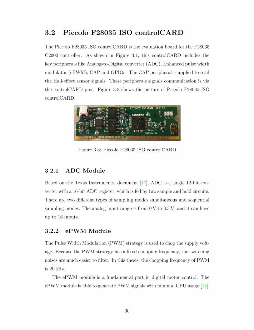
3.2 Piccolo F28035 ISO controlCARD

The Piccolo F28035 ISO controlCARD is the evaluation board for the F28035

C2000 controller. As shown in Figure 3.1, this controlCARD includes the

key peripherals like Analog-to-Digital converter (ADC), Enhanced pulse width

modulator (ePWM), CAP and GPIOs. The CAP peripheral is applied to read

the Hall-effect sensor signals. These peripherals signals communication is via

the controlCARD pins. Figure 3.3 shows the picture of Piccolo F28035 ISO

controlCARD.

Figure 3.3: Piccolo F28035 ISO controlCARD

3.2.1 ADC Module

Based on the Texas Instruments’ document [17], ADC is a single 12-bit con-

verter with a 16-bit ADC register, which is fed by two sample and hold circuits.

There are two different types of sampling modes:simultaneous and sequential

sampling modes. The analog input range is from 0 V to 3.3 V, and it can have

up to 16 inputs.

3.2.2 ePWM Module

The Pulse Width Modulation (PWM) strategy is used to chop the supply volt-

age. Because the PWM strategy has a fixed chopping frequency, the switching

noises are much easier to filter. In this thesis, the chopping frequency of PWM

is 20 kHz.

The ePWM module is a fundamental part in digital motor control. The

ePWM module is able to generate PWM signals with minimal CPU usage [18].

30

For the BLDC motor control, three ePWM modules are needed to generate

six PWM signals for the three-phase inverter.

In this thesis, one high side transistor is switched on and off according to

the control signals, and one low side transistor is left on. This mode is able to

reduce the switching losses and torque ripples.

3.3 DRV8312 Digital Motor Control Board

The DRV8312 DMC board is the motor driver board. The key component

is the DRV8312 which is a three-phase motor driver. On the DRV8312 DMC

board, some macros to implement different functions in the BLDC motor driver

system are included. In this section, an introduction will be made to the

DRV8312 DMC board based on the documents [15][16].

3.3.1 DRV8312

Because the BLDC motor is not self-commutated, the stator coils will be

energized in a predefined order to make the rotor rotate. The stator coils

needs to be powered by the external device. For a three-phase BLDC motor,

normally a three-phase inverter is used to power the stator coils. Figure 3.1

shows the diagram of the inverter. The Piccolo F28035 controlCARD will send

PWM control signals to the three-phase inverter.

DRV8312 is a three-phase BLDC motor driver in the Texas Instrument

DRV83x2 driver family. The DRV8312 is able to be applied in the energy-

efficient areas, because it has high energy efficiency which can reach maximum

97 %. In order to power DRV8312, two different power supplies are needed,

one at 12 V for gate-drive voltage supply and power supply for digital voltage

regulator, and another up to 50 V for power supply input for half-bridges [15].

The PWM switching operating frequency of the DRV8312 can be up to

500 kHz. This driver has an advanced protection system which can protect the

device from different fault conditions that could make a damage to the hard-

wares. The protection system includes the bootstrap capacitor undervoltage

protection which can protect the device from the possible damage caused low

31

switching frequency operation, overload protection, and short circuit protec-

tion. The overcurrent detectors allow users to set the current limits based on

the application requirements, and the current-limiting circuit will prevent the

BLDC motor from possible damage caused by overcurrent.

3.3.2 Macro Blocks

On the DRV8312 DMC board, there are several macro blocks to implement

different functions. The DC bus connection macro block provides DC bus

power for the control board. There are two options for the connection block:

one is using the power entry jack to connect a 24 V AC/DC supply, and another

is using PVDD/GND terminals to connect a different power supply.

From Figure 3.1, the DRV8312 DMC board can be connected with a BLDC

motor, and it can also receive the Hall-effect sensors or Quadrature Encoder

signals. The motor connection block is to connect the BLDC motor wires [16].

The Quadrature Encoder connection block can be applied to connect a shaft

encoder to receive motor positions information. Hall-effect sensor connection

block can be used to connect to the Hall-effect sensors. In this thesis, the

signals from the Hall-effect sensor connection block is applied to verify the

accuracy of the sensorless commutation methods.

From Figure 3.1, the DRV8312 DMC board has the terminal voltage sensing

block to measure the three phase terminal voltages Va, Vb and Vc. The terminal

voltages are measured by taking ground as the referenced point. The details

about the terminal voltage sensing block will be introduced in Chapter 4. The

current sensing block is to measure the BLDC motor currents. Ia, Ib and Ic

are the phase currents, and IDC are the DC bus current. In order to measure

the motor current, a reference voltage of 1.65 V is required. This reference

voltage can be provided by a voltage follower. On the DRV8312 DMC board,

the voltage follower circuit is applied to generate a 1.65 V reference voltage

from the 2.5 V voltage source.

A differential amplifier circuit is applied to convert the current input to

an output voltage from 0 to 3.3 V. Figure 3.4 shows the differential amplifier

circuit on the DRV8312 DMC board. The reference voltage 1.65 V is provided

32

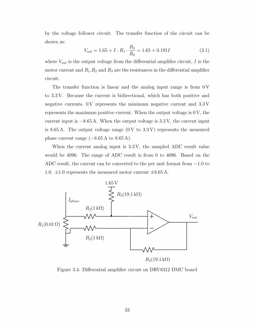
by the voltage follower circuit. The transfer function of the circuit can be

shown as:

Vout = 1.65 + I ·R1 ·R3

R2

= 1.65 + 0.191I (3.1)

where Vout is the output voltage from the differential amplifier circuit, I is the

motor current and R1,R2 and R3 are the resistances in the differential amplifier

circuit.

The transfer function is linear and the analog input range is from 0 V

to 3.3 V. Because the current is bidirectional, which has both positive and

negative currents, 0 V represents the minimum negative current and 3.3 V

represents the maximum positive current. When the output voltage is 0 V, the

current input is −8.65 A. When the output voltage is 3.3 V, the current input

is 8.65 A. The output voltage range (0 V to 3.3 V) represents the measured

phase current range (−8.65 A to 8.65 A).

When the current analog input is 3.3 V, the sampled ADC result value

would be 4096. The range of ADC result is from 0 to 4096. Based on the

ADC result, the current can be converted to the per unit format from −1.0 to

1.0. ±1.0 represents the measured motor current ±8.65 A.

1.65 V

R3(19.1 kΩ)

Vout

Iphase

R3(19.1 kΩ)

R2(1 kΩ)

R2(1 kΩ)

R1(0.01 Ω)

Figure 3.4: Differential amplifier circuit on DRV8312 DMC board

33

3.3.3 Power Domains of the Kit

There are two power domains on this kit. One is the low voltage domain,

which is used to provide power for the F28035 C2000 controller and the logic

circuits. The low voltage domain has three levels voltages: 3.3 V, 5 V and

12 V. The low voltage domain can be sourced from two areas: one is the 12 V

DC control power entry, which needs external power supply, and another is

the on board buck regular, which will regulate the DC bus power to 12 V.

Another power domain is the medium voltage power domain, which will

provide medium voltages to the three-phase inverter. The medium voltages

are called the DC bus voltages. The three-phase inverter will provide power

to the BLDC motor and the medium voltages can be up to 52.5 V.

For each phase of the BLDC motor, an individual switch is used to deter-

mine the control mode of that phase. The switch can be manually set to three

positions. If the switch is in the middle position, the switch will be controlled

by a GPIO signal. If the switch is in the up position, the half-bridge output

will be enabled. If the switch is in the down position, the half-bridge output

will be disabled.

3.3.4 PWMDAC Module

The PWMDAC module can be applied to view the measurements waveforms

on an oscilloscope. To get the actual low frequency signals, a first order low-

pass filter is used to filter out the high frequency components. The PWMDAC

module can be used to observe three different signals at one time. The low-

pass filter time constant (τ) and cut-off frequency (fc) can be calculated using

following equations:

τ = R · C = 2.21× 10−4 s (3.2)

fc =1

2πτ= 720.5 Hz (3.3)

where R is the low-pass filter resistance and C is the low-pass filter capac-

itance.

34

3.4 BLDC Motor

Figure 3.5 shows the BLDC motor used in this thesis, which is made by Ana-

heim Automation and its model number is BLY172S-24V-4000. This BLDC

motor is a cost effective solution to the velocity control application. This mo-

tor has 4 pairs of rotor poles and three wires for the phases and five wires for

the hall sensors. Table 3.1 shows the motor specifications.

Parameter ValuesP 8R 0.4 ΩL 0.6 mHzKt 0.041 Nm/AKe 3.35 V/kRPMJ 48 g − cm2

Table 3.1: BLDC motor specifications

Figure 3.5: BLY172S-24V-4000 motor

3.5 Summary

In this chapter, we present the experimental environment in this thesis. An

introduction is made to the Piccolo F28035 controlCARD, the DRV8312 DMC

board and also the basic macro blocks. Finally, we make a discussion on the

BLDC motor and its parameters.

35

Chapter 4

Sensorless BLDC Motor DriveBased on Line VoltageDifferences

In this chapter, a sensorless BLDC motor control method based on line voltage

differences [6] is introduced and verified through experiment. As introduced

in Chapter 1, methods based on line voltage differences can eliminate the

requirement for the motor neutral voltage, which will increase the accuracy of

the commutation strategy.

4.1 Six-step Commutation

The six-step commutation is the most commonly used way to commutate a

BLDC motor. Figure 4.1 shows the stator space sectors diagram. A and

X represent the stator windings of phase A. B and Y represent the stator

windings of phase B. C and Z represent the stator windings of phase C. A−X,

B − Y and C − Z separate the space into six 60 sectors.

4.1.1 Analysis of Six-step Commutation

The six sectors represents six states of a BLDC motor. If Hall-effect sensors are

used to detect rotor positions, for each of the six states, three-digit numbers

based on the three Hall-effect sensors’ signals are used to represent the cur-

rent rotor position. When the rotor moves to the next sector, the three-digit

numbers will change to a different set of three-digit numbers representing the

36

A

Z

B

X

C

Y

5

01

2

3 4

Figure4.1:Statorspacesectorsdiagram

newstate.Forsensorlesscontrolmethods,differenttechniqueswillbeusedto

estimaterotorpositions.

Assumingthattherotorisinsector0,thecurrentdirectionofphaseAis

fromAtoX.thecurrentdirectionofphaseBisfromYtoBandphaseCis

floating.NowthestatorfieldisinthedirectionofC−ZasshowninFigure

4.2(a),anditwillwilldrivetherotortomovetosector1.

Afterrotormovesintosector1,thecurrentdirectionofphaseAisfromA

toX.thecurrentdirectionofphaseCisfromZtoCandphaseBisfloating.

ThestatorcurrentsshapethestatorfieldwhichisinthedirectionofB−Y

asshowninFigure4.2(b).Torquewillbegeneratedbasedonthephaseshift

betweentherotorfieldandthestatorfield. Thenthetorquewilldrivethe

rotortomovetosector2.

Insector2,thecurrentdirectionofphaseCisfromZtoC.Thecurrent

directionofphaseBisfromBtoYandphaseAisfloating.Thestatorfield

isinthedirectionofA−XasshowninFigure4.2(c),anditwilldrivethe

rotortomovetosector3.

Insector3,thecurrentdirectionofphaseAisfromXtoA.Thecurrent

directionofphaseBisfromBtoYandphaseCisfloating.Thestatorfield

37

is in the direction of C − Z as shown in Figure 4.2(d), and it will will drive

the rotor to move to sector 4.

In sector 4, the current direction of phase A is from X to A. The current

direction of phase C is from C to Z and phase B is floating. The stator field

is in the direction of B − Y as shown in Figure 4.2(e), and it will drive the

rotor to move to sector 4.

In sector 5, the current direction of phase C is from C to Z. The current

direction of phase B is from Y to B and phase A is floating. The stator field

is in the direction of A − X as shown in Figure 4.2(f), and it will drive the

rotor to move to sector 0.

As analyzed above, the stator field moves in a discrete step of 60 electrical

degrees. The torque will continuously drive the rotor to rotate. Because the

phase shift between the rotor field and the stator field will change when the

rotor is rotating, this shift will cause torque ripples. The torque ripples can be

reduced if the field oriented control is applied. Then the phase shift between

the rotor field and the stator field is fixed to be 90 electrical degrees to generate

the maximum torque.

The commutation state pointer input (0 to 5) indicates one of the six states.

During each state, only two phases are conducting so two switches are active

and the other four will be turned off. If the commutation state pointer is

equal to 0, current flows from phase A to phase B. Table 4.1 shows the six

commutation states of the BLDC motor.

Commutation States ia ib ic

0 positive negative floating1 positive floating negative2 floating positive negative3 negative positive floating4 negative floating positive5 floating negative positive

Table 4.1: Commutation states in six-step BLDC motor control

38

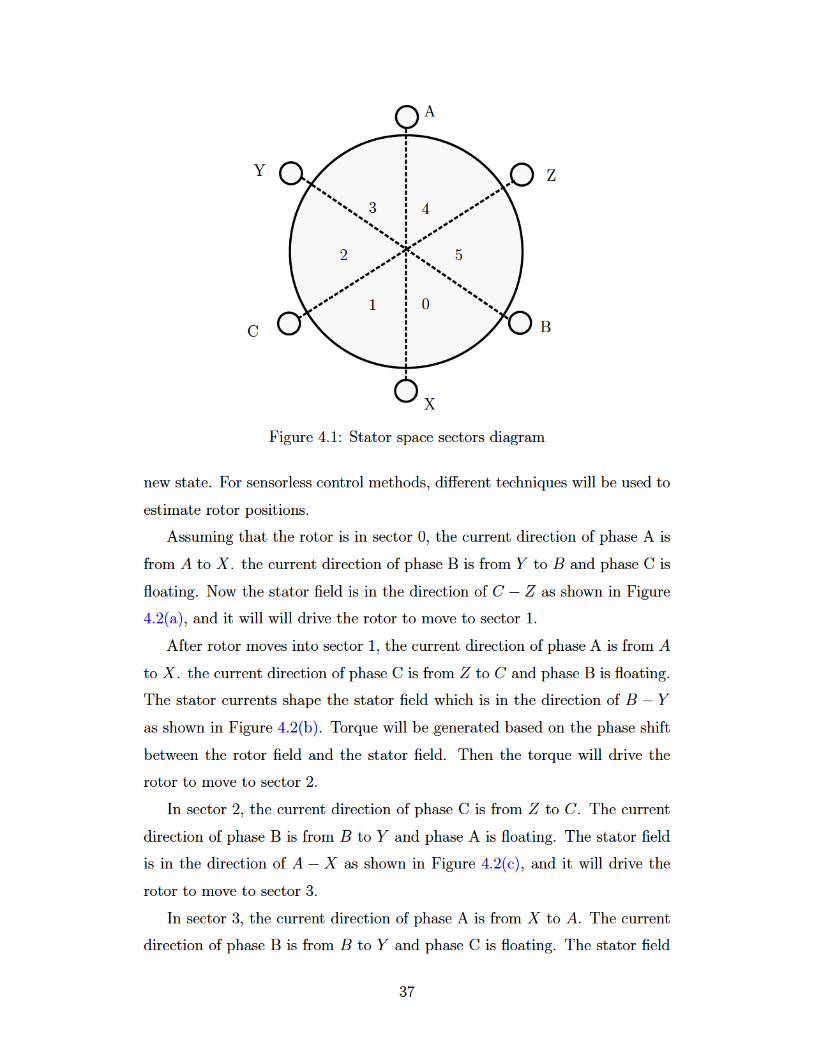
A

Z

B

X

C

Y

×

·

×

·N

S

Fstator

(a)Sector0

A

Z

B

X

C

Y

×

.

×

. N

S

Fstator

(b)Sector1

A

Z

B

X

C

Y . ×

.

N S

Fstator

×

(c)Sector2

A

Z

B

X

C

Y .

×

.

N

S

Fstator

×

(d)Sector3

A

Z

B

X

C

Y

×

.

N

S

Fstator

×

.

(e)Sector4

A

Z

B

X

C

Y×

.

NS

Fstator

×

.

(f)Sector5

Figure4.2:BLDCmotorsix-stepcommutation

39

4.2 Sensorless Commutation Method Based on

Line Voltage Differences

In this section, a sensorless control method using the six-step commutation

sequence will be introduced. The proposed method are based on the work in

[6].

For the BLDC motor we used, stator windings of three phases are connected

in star. The terminal voltage of phase A referenced with the motor neutral

voltage is Van as:

Van = Ria + Ldiadt

+ ea (4.1)

Similarly, terminal voltages of phase B and phase C are Vbn and Vcn as:

Vbn = Rib + Ldibdt

+ eb (4.2)

Vcn = Ric + Ldicdt

+ ec (4.3)

where Van, Vbn and Vcn are the phase voltages referenced to the motor neutral

voltage, L is the phase stator inductance, R is the phase stator resistance, ia,

ib and ic are the phase currents and ea, eb and ec are the phase back-EMFs.

On DRV8312 DMC board, the terminal voltages are measured by taking

ground as the referenced point. The line voltage Vab of the terminal voltages

can be calculated as:

Vab = R(ia − ib) + Ld(ia − ib)

dt+ ea − eb (4.4)

Similarly, terminal line voltages Vbc and Vca are shown below:

Vbc = R(ib − ic) + Ld(ib − ic)

dt+ eb − ec (4.5)

Vca = R(ic − ia) + Ld(ic − ia)

dt+ ec − ea (4.6)

From equations above, the line voltages can be calculated based on the

terminal voltages measured with respect to ground, so the requirement for

motor neutral voltage is eliminated.

40

We can calculate the line voltage differences based on the line voltages

equations above. The line voltage difference Vbcab can be calculated as:

Vbcab = Vbc − Vab

= R(2ib − ia − ic) + Ld(2ib − ia − ic)

dt+ 2eb − ea − ec

(4.7)

Similarly, Vabca and Vcabc can be calculated as:

Vabca = Vab − Vca

= R(2ia − ib − ic) + Ld(2ia − ib − ic)

dt+ 2ea − eb − ec

(4.8)

Vcabc = Vca − Vbc

= R(2ic − ia − ib) + Ld(2ic − ia − ib)

dt+ 2ec − ea − eb

(4.9)

If the commutation state pointer is equal to 0, the stator current flows from

phase A to phase B. Because phase C is open, the phase C current ic = 0.

Phase A current ia and phase B current ib have the same magnitude but

opposite. From Figure 2.1 [23], phase A back-EMF ea and phase B back-EMF

eb also have the same magnitude but opposite. The relationships can be shown

as:

ia + ib = 0 (4.10)

ea + eb = 0 (4.11)

When the commutation state pointer is equal to 0, the line voltage differ-

ence Vcabc can be calculated as:

Vcabc = Vca − Vbc = 2ec − ea − eb = 2ec (4.12)

From the equation above, the line voltage difference Vcabc is equal to an

amplified phase C back-EMF value and the gain is two. So we can use line

voltage differences to estimate zero-crossing points of back-EMFs. Theoreti-

cally, when the commutation state pointer is equal to 0, Vcabc starts from the

maximum positive value and goes to the minimum negative value. Because

the back-EMF waveform changes linearly, the zero-crossing point will occur in

the middle of the commutation state 0. As each state contains 60 electrical

degrees, a 30 offset exists between the back-EMFs’ zero-crossing points and

the current commutation instants.

41

Similarly, when the commutation state pointer is equal to 3, the stator

current flows from phase B to phase A and phase C is open. Vcabc has the

same expression as in commutation state 0. The difference is that Vcabc starts

from the minimum negative value and goes to the maximum positive value.

In commutation state 1, the stator current flows from phase A to phase C,

and phase B is open. In commutation state 4, the stator current flows from

phase C to phase A and phase B is open. The phase B current ib = 0. Phase A

current ia and phase C current ic are equal and opposite. Phase A back-EMF

ea and phase C back-EMF ec are also equal and opposite. The line voltage

difference Vbcab can be calculated as:

Vbcab = Vbc − Vab = 2eb − ea − ec = 2eb (4.13)

In commutation state 2, the stator current flows from phase B to phase

C, and phase A is open. In commutation state 5, the stator current flows

from phase C to phase B, and phase A is open. The phase A current ib = 0.

Phase B current ib and phase C current ic are equal and opposite. Phase B

back-EMF eb and phase B back-EMF ec are also equal and opposite. The line

voltage difference Vabca can be calculated as:

Vabca = Vab − Vca = 2ea − eb − ec = 2ea (4.14)

To validate the proposed sensorless method, the relationship between the

line voltage differences and back-EMFs is verified in Matlab/Simulink envi-

ronment. For a real BLDC motor, the back-EMF waveform shape cannot be

ideal trapezoidal, which is the reason why the back-EMF voltage constant is

less than the torque constant for the BLDC motor used in the experimental

environment. The BLDC motor model for simulation has ideal trapezoidal

back-EMFs, and we choose the the torque constant to be same as the back-

EMF voltage constant instead of the one in Table 3.1. Except for the torque

constant, the BLDC motor in the Simulink model has the same parameters in

Table 3.1.

The line voltage differences are represented by the expressions of back-

EMFs to validate the zero-crossing points match. Figure 4.3 shows the simu-

lation results of the line voltage differences and back-EMFs waveforms. From

42

0.6 0.62 0.64 0.66 0.68 0.7−10

0

10

20

time (s)

Voltage (V

)

0.6 0.62 0.64 0.66 0.68 0.7−10

0

10

20

time (s)

Voltage (V

)

0.6 0.62 0.64 0.66 0.68 0.7−10

0

10

20

time (s)

Voltage

(V)

2ea − eb − ecea

2eb − ea − eceb

2ec − ea − ebec

Figure 4.3: Simulations results of the line voltage differences and back-EMFswaveforms at 700 rpm with 0.04 Nm load

the simulation results, we can see that at the zero-crossing points, the corre-

sponding line voltage difference is an amplified back-EMF, and the line voltage

differences have the same zero-crossing points as the back-EMFs.

In each state, one line voltage difference is applied to estimate the zero-

crossing points of the corresponding back-EMF waveform. A combined com-

mutation function is applied to estimate all the zero-crossing points of back-

EMFs as shown in Table 4.2. Table 4.2 also shows the polarity of the zero-

crossing points.

The combined commutation function can be shown in Figure 4.4. The

simulation results show that the combined commutation function has the same

zero-crossing points as the back-EMFs, which verifies the correctness of the

combined commutation function. The combined commutation function will be

applied in the experiment environment.

43

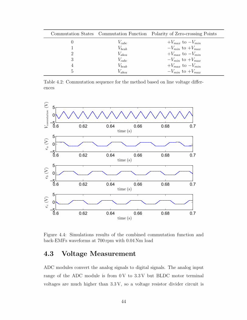
Commutation States Commutation Function Polarity of Zero-crossing Points

0 Vcabc +Vmax to −Vmin

1 Vbcab −Vmin to +Vmax

2 Vabca +Vmax to −Vmin

3 Vcabc −Vmin to +Vmax

4 Vbcab +Vmax to −Vmin

5 Vabca −Vmin to +Vmax

Table 4.2: Commutation sequence for the method based on line voltage differ-ences

0.6 0.62 0.64 0.66 0.68 0.7−5

0

5

time (s)

Vcommtation(V

)

0.6 0.62 0.64 0.66 0.68 0.7−5

0

5

time (s)

ea(V

)

0.6 0.62 0.64 0.66 0.68 0.7−5

0

5

time (s)

eb(V

)

0.6 0.62 0.64 0.66 0.68 0.7−5

0

5

time (s)

ec(V

)

Figure 4.4: Simulations results of the combined commutation function andback-EMFs waveforms at 700 rpm with 0.04 Nm load

4.3 Voltage Measurement

ADC modules convert the analog signals to digital signals. The analog input

range of the ADC module is from 0 V to 3.3 V but BLDC motor terminal

voltages are much higher than 3.3 V, so a voltage resistor divider circuit is

44

used to convert the terminal voltage to fit the analog input range of ADC

module.

Because of the inverter switching, BLDC motor terminal voltages contain

some high frequency harmonics. In order to eliminate the harmonics, a first-

order low pass filter is included in the voltage resistor divider circuit as shown

in Figure 4.5.

Vin

R1

R2

Vout

C

Figure 4.5: Voltage resistor divider circuit

The transfer function of the low pass filter is:

VoutVin

=R2

R1 +R2 +R1R2Cs(4.15)

where C is the low pass filter capacitance, R1 and R2 are the voltage divider

resistances, Vout is the filtered waveform of Vin.

Table 4.3 shows the parameters of the motor terminal voltage sensing cir-

cuit.

4.4 Phase Delay Compensation

From the analysis above, line voltage differences can be used to estimate the

zero-crossing points of back-EMFs. Because a 30 offset exists between the

45

Parameter Values

R1 95.3 kΩR2 4.99 kΩC 0.047 µF

Table 4.3: Terminal voltage sensing circuit specifications

back-EMFs’ zero-crossing points and the current commutation instants, a 30

phase shift should be made to ensure the correct operation of the motor.

However, because of the phase delay caused by the low pass filter, the actual

offset between the measured zero-crossing point of back-EMFs and current

commutation instants is not exactly 30. The delayed angle caused by the

first-order low pass filter can be calculated as:

θ = − tan−1(R1 ·R2 · C · ωe

R1 +R2

) (4.16)

ωe =2π

T(4.17)

where T is one electrical period and ωe is the synchronous speed of the BLDC

motor.

Due to the delayed angle caused by the low pass filter, the electrical degree

offset φ between the zero-crossing points of back-EMFs and current commu-

tation instants should be modified as

φ = 30 − θ (4.18)

Figure 4.6 shows the software flowchart of the proposed sensorless commu-

tation method with phase delay compensation. In order to calculate the φ in

software, the electrical period needs to be calculated. As the current electrical

period is unknown, the difference between two adjacent electrical periods is

small enough to ignore, so the last electrical period T is applied to calculate

Tdelay. At the beginning of state 5, T will be calculated based on the time

difference between the current time and the beginning time of state 5 in the

last electrical period. The phase delay time will be calculated and then used

in the next electrical period:

Tdelay =φ

360· T (4.19)

46

where T is the last electrical period and φ is the phase delay angle calculated

at the end of last electrical period.

For each commutation state, the time counter will start after detecting the

zero-crossing point of the corresponding line voltage difference. When the time

counter is equal to Tdelay, this point is treated as the commutation instant and

the BLDC motor will switch to the next state.

As mentioned in Chapter 2, the relationship between electrical frequency

and mechanical frequency is

fe =p

2fm (4.20)

fm =Nrpm

60(4.21)

where p is the number of poles, fm is the mechanical frequency, fe is the

electrical frequency and Nrpm is rotor speed in rpm.

The electrical period T from the commutation method will be applied to

estimate Nrpm as shown in equation below:

Nrpm = 60fm = 60 · 2

pfe

=120

Tp

(4.22)

From the analysis above, the delayed angle caused by the low pass filter

has a positive relationship with the motor rotor speed. If the BLDC motor

speed is 1000 rpm, the delayed angle caused by the low pass filter is 5.33 using

the equation below:

θ = tan−1(R1 ·R2 · C · ωe

R1 +R2

)

= tan−1(R1 ·R2 · CR1 +R2

· πpNrpm

60)

(4.23)

When the speed is low or medium, the delayed angle won’t cause a com-

mutation mistake. But when motor speed is high, the delayed angle will cause

problems. Some compensation needs to be done to guarantee the correct op-

eration of BLDC motors. In this thesis, F28035 C2000 controller will be used

to compensate the phase delay φ, so the current commutation instants can be

in phase with the zero-crossing points of line voltage differences.

47

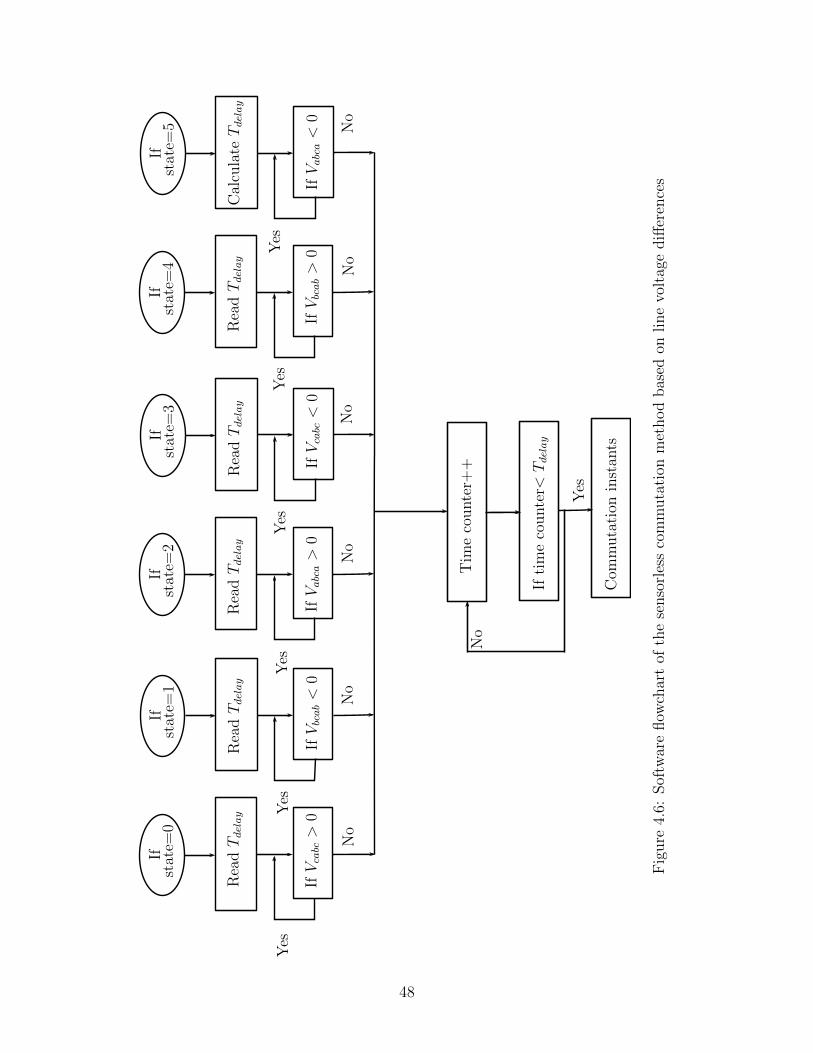
Rea

dTdelay

IfVca

bc>

0

Tim

eco

unte

r++

Ifti

me

counte

r<Tdelay

Com

muta

tion

inst

ants

Yes

No

Ifst

ate=

0

Rea

dTdelay

IfVbcab<

0

Ifst

ate=

1

Rea

dTdelay

IfVabca>

0

Ifst

ate=

2

Rea

dTdelay

IfVca

bc<

0

Ifst

ate=

3

Rea

dTdelay

IfVbcab>

0

Ifst

ate=

4

Cal

cula

teTdelay

IfVabca<

0

Ifst

ate=

5

No

No

No

No

No

No

Yes

Yes

Yes

Yes

Yes

Yes

Fig

ure

4.6:

Sof

twar

eflow

char

tof

the

senso

rles

sco

mm

uta

tion

met

hod

bas

edon

line

volt

age

diff

eren

ces

48

4.5 Starting Procedure

For BLDC control methods with Hall-effect sensors or Quadrature Encoder

signals, it is not a problem for a BLDC motor to start up. For back-EMF

based methods like the method used in this chapter, back-EMFs’ values are

needed to achieve the position estimation. However, back-EMFs’ values are

zero during standstill, and they are also very small when the motor speed is

low.

Normally, a starting procedure is required for the methods based on back-

EMFs. In this chapter, the BLDC motor will be started blindly using the

conventional open-loop starting method [8].

During the first stage, any two phases of stator windings will be energized.

In this thesis, the stator current will firstly flow from phase A to phase B. The

stator currents will generate a flux whose amplitude and direction are both

constant. The stator flux will attract the rotor to point in the same direction,

so the rotor is forced to align at a predefined position [8]. Then, the stator

current flows from phase A to phase C so the BLDC motor will be in the

next state. The stator flux will point to a new direction, so the rotor will be

attracted to move to the next position. During this open-loop starting mode,

the stator windings will be energized in a predefined order:

AB → AC → BC → BA→ CA→ CB

When the BLDC motor speeds up, back-EMFs will also increase. When the

zero-crossing points of back-EMFs can be stably detected, the control system

will switch to the sensorless mode.

4.6 Electrical Noises

The noises included in the calculated line voltage difference waveforms may

cause false zero-crossing points detection. The main noises are from the

chopped pulses generated by PWM. Spikes caused by the free-wheeling diode

conduction current are another source [6].

49

Assuming that the BLDC motor is in commutation state 1, now it will

switch to state 2. During commutation state 1, the upper transistor of phase

A (T1) and the lower transistor of phase C (T6) are on. At the commutation

instant, T1 will be turned off and the upper transistor of phase B (T3) will

be turned on. The stator current continues to flow through the free-wheeling

diode of phase A and decreases.

The free-wheeling current will cause spikes in the calculated line voltage

difference waveforms. The spikes may cross the zero thus cause false zero-

crossing points detection.

According to the reference [6], the free-wheeling current during time is

much smaller than the phase delay time Tdelay, so the spike will disappear

before the back-EMFs cross zero.

The calculated line voltage difference waveforms also contains noises from

the sensing circuit. For DRV8312-C2 kit, each terminal voltage is sensed with

a voltage resistor divider and a first order low pass filter. The sensing circuit

may bring noises to the measured terminal voltages so it will also affect the

line voltage differences.

Because the virtual neutral voltage is not used in this method, it will reduce

the affect of electrical noises. The low pass filter of the terminal voltage sensing

circuit can filter out the chopped pulses generated by PWM, but the calculated

line voltage difference waveforms still contain some noises which may cause

false zero-crossing points detection. In order to minimize the influence of the

noises, a counter can be used to calculate how many times the measured line

voltage difference value crosses zero [38]. The noises only remain for a very

short time. If the counter reaches a predefined value, this point is treated as

the real zero-crossing point of the line voltage difference. Otherwise, it will be

treated as noises and will not trigger the commutation to the next state.

4.7 Proposed Sensorless Drive

Assuming that ω is the estimated motor speed and ωref is the reference motor

speed, a proportional integral (PI) controller is applied to determine the duty

50

cycle of the PWM signals based on the difference between ω and ωref . Figure

4.7 shows the proposed sensorless drive for speed control of a BLDC motor.

The measured three phase terminal voltages are the inputs of the line

voltage differences calculation block. The calculated line voltage differences

and the motor speed are the inputs of the commutation trigger block. At the

beginning of each electrical period, the phase delay time will be calculated,

and it will be used in this electrical period.

Three-phaseinverter

Commutation

T

−PI

ωref

ω

+Duty Cycle BLDC Motor

Commutation State

Vcabc, Vbcab, Vabca

BLDC PWMDrive

PWM Signals

Method inFigure 4.6

Speed Estimationusing (4.22)

Figure 4.7: Proposed sensorless BLDC motor drive based on line voltage dif-ferences

4.8 Experimental Results

In this section, we presents the experiment results of the proposed sensorless

BLDC motor drive based on line voltage differences at different speeds, and

the effectiveness of the compensation method is also verified and analyzed.

4.8.1 Experiment Results at 600 rpm

Figure 4.8 shows the measured line voltage differences at 600 rpm. Figure 4.9

shows the speed response at 600 rpm, and the error is calculated using the

equation below:

error(%) =|ω − ωref |ωref

× 100% (4.24)

51

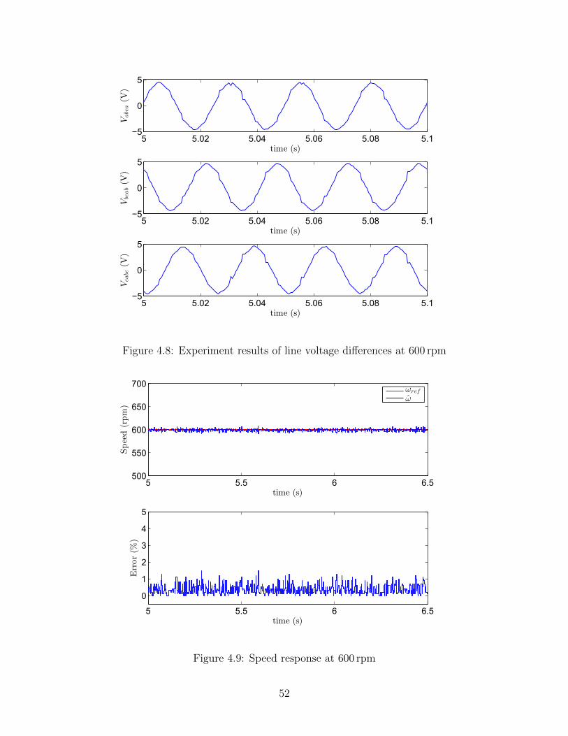
5 5.02 5.04 5.06 5.08 5.1−5

0

5

time (s)

Vabca(V

)

5 5.02 5.04 5.06 5.08 5.1−5

0

5

time (s)

Vbcab(V

)

5 5.02 5.04 5.06 5.08 5.1−5

0

5

time (s)

Vcabc(V

)

Figure 4.8: Experiment results of line voltage differences at 600 rpm

5 5.5 6 6.5500

550

600

650

700

time (s)

Speed(rpm)

ωref

ω

5 5.5 6 6.5

0

1

2

3

4

5

time (s)

Error(%

)

Figure 4.9: Speed response at 600 rpm

52

4.8.2 Experiment Results at 1000 rpm

Figure 4.10 shows the measured line voltage differences at 1000 rpm. Figure

4.11 shows the speed response at 1000 rpm.

Based on the results in subsection 4.8.1 and subsection 4.8.2, we can see

that the line voltage differences waveforms are symmetric, and the speed of

the BLDC motor can remain stable with negligible error.

When the BLDC motor runs in open-loop commutation mode, there is a

big acoustic noise from the motor due to its inaccuracy commutation. During

the sensorless commutation mode, the acoustic noise is reduced.

10.9 10.91 10.92 10.93 10.94 10.95 10.96−10

0

10

time (s)

Vabca(V

)

10.9 10.91 10.92 10.93 10.94 10.95 10.96−10

0

10

time (s)

Vbcab(V

)

10.9 10.91 10.92 10.93 10.94 10.95 10.96−10

0

10

time (s)

Vcabc(V

)

Figure 4.10: Experiment results of line voltage differences at 1000 rpm

4.8.3 Phase Delay Compensation

For the trapezoidal control of BLDC motors, back-EMFs are required to be in

phase with the phase current. In this section, we will make comparison of the

proposed sensorless drive with and without phase delay compensation. From

the experiment results, the phase delay compensation method does not make

a big difference if the BLDC motor works in low or medium speeds. However,

53

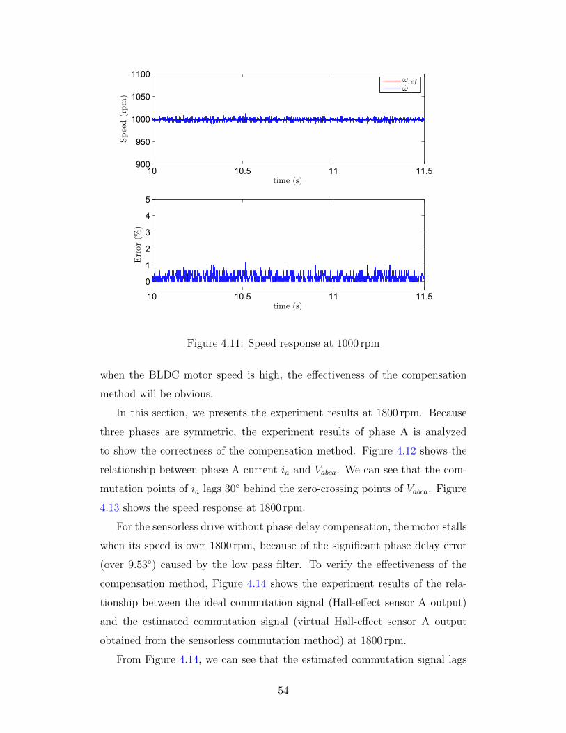
10 10.5 11 11.5900

950

1000

1050

1100

time (s)

Speed(rpm)

10 10.5 11 11.5

0

1

2

3

4

5

time (s)

Error(%

)

ωref

ω

Figure 4.11: Speed response at 1000 rpm

when the BLDC motor speed is high, the effectiveness of the compensation

method will be obvious.

In this section, we presents the experiment results at 1800 rpm. Because

three phases are symmetric, the experiment results of phase A is analyzed

to show the correctness of the compensation method. Figure 4.12 shows the

relationship between phase A current ia and Vabca. We can see that the com-

mutation points of ia lags 30 behind the zero-crossing points of Vabca. Figure

4.13 shows the speed response at 1800 rpm.

For the sensorless drive without phase delay compensation, the motor stalls

when its speed is over 1800 rpm, because of the significant phase delay error

(over 9.53) caused by the low pass filter. To verify the effectiveness of the

compensation method, Figure 4.14 shows the experiment results of the rela-

tionship between the ideal commutation signal (Hall-effect sensor A output)

and the estimated commutation signal (virtual Hall-effect sensor A output

obtained from the sensorless commutation method) at 1800 rpm.

From Figure 4.14, we can see that the estimated commutation signal lags

54

10.8 10.805 10.81 10.815 10.82−20

−15

−10

−5

0

5

10

15

20

Vabca(V

)

time (s)10.8 10.805 10.81 10.815 10.82

−1

0

1

ia(A

)

Figure 4.12: Phase A current and Vabca at 1800 rpm

10 10.5 11 11.51700

1750

1800

1850

1900

time (s)

Speed(rpm)

10 10.5 11 11.5

0

1

2

3

4

5

time (s)

Error(%

)

ωref

ω

Figure 4.13: Speed response at 1800 rpm

55

0 0.005 0.01 0.015 0.02

0

1

Estim

atedsignal(V

)

time (s)

Before compensation

0 0.005 0.01 0.015 0.02

0

1

Estim

atedsignal(V

)

time (s)

After compensation

0 0.005 0.01 0.015 0.020

2

4

Idealsignal(V

)

0 0.005 0.01 0.015 0.020

2

4

Idealsignal(V

)

Figure 4.14: Ideal commutation signal and estimated commutation signal at1800 rpm

behind the ideal commutation signal and the phase delay is significant. After

phase delay compensation, the estimated commutation signal matches well

with the ideal commutation signal.

Before phase compensation, the acoustic noise is noticeable due to inaccu-

racy commutation. After phase compensation, the acoustic noise is reduced.

Based on the analysis above, we can conclude that phase delay compen-

sation is necessary for high speed region. With phase delay compensation,

the high speed capability of BLDC motors can be improved, and the acoustic

noise from the motor will be reduced. The estimated commutation signal is

precise enough to replace the ideal commutation signal, so it can be applied

to realize sensorless commutation.

56

4.9 Summary

In this chapter, we make a detailed analysis on the six-step commutation

of the BLDC motors. Then we discuss the sensorless commutation method

based on line voltage differences, and it is validated by the simulation results.

The sensorless commutation method with phase delay compensation is further

implemented in the experimental environment.

57

Chapter 5

Sensorless BLDC Motor DriveBased on Disturbance Observer

In Chapter 4, a sensorless control method based on terminal line voltage differ-

ences is introduced and verified through experiment. However, this sensorless

method requires a 30 phase shift to acquire the correct commutation instants,

which lowers the accuracy of the commutation method. The complexity of the

sensorless control method is also increased. In this chapter, a sensorless control

method based on the disturbance observer will be discussed, and this method

does not require a 30 phase shift [39].

5.1 Disturbance Observer

The disturbance observer has been widely applied in the motion control area

because of its ability to implement disturbance rejection and compensate the

plant uncertainties. The Disturbance Estimating Filter (DEF) disturbance

observer is introduced in [33].

The DEF disturbance observer is proposed based on the two-degree-of-

freedom controller. For the two-degree-of-freedom controller, one degree-of-

freedom is to implement disturbance rejection, and another is to design the ref-

erence response. The normal structure of DEF disturbance observer is shown

in Figure 5.1 [33]. The actual plant transfer function is P ′(s) and the nominal

plant transfer function is P (s).

ui is the input signal and d is the disturbance signal. The actual input

58

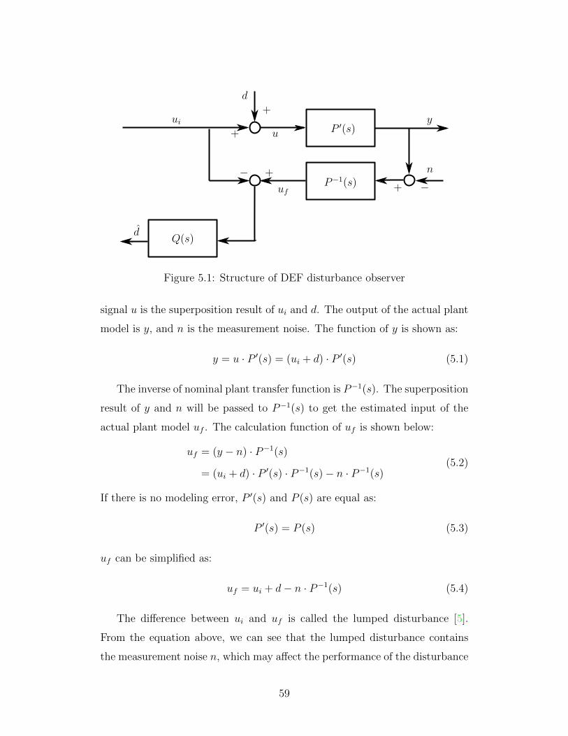
ui

d

u P ′(s)

P−1(s)

y

n

Q(s)

+

+

+ −+−uf

d

Figure 5.1: Structure of DEF disturbance observer

signal u is the superposition result of ui and d. The output of the actual plant

model is y, and n is the measurement noise. The function of y is shown as:

y = u · P ′(s) = (ui + d) · P ′(s) (5.1)

The inverse of nominal plant transfer function is P−1(s). The superposition

result of y and n will be passed to P−1(s) to get the estimated input of the

actual plant model uf . The calculation function of uf is shown below:

uf = (y − n) · P−1(s)

= (ui + d) · P ′(s) · P−1(s)− n · P−1(s)(5.2)

If there is no modeling error, P ′(s) and P (s) are equal as:

P ′(s) = P (s) (5.3)

uf can be simplified as:

uf = ui + d− n · P−1(s) (5.4)

The difference between ui and uf is called the lumped disturbance [5].

From the equation above, we can see that the lumped disturbance contains

the measurement noise n, which may affect the performance of the disturbance

59

observer. The frequency of the measurement noise is usually high, and the

frequency of disturbance signal is low [5].

A low pass filter Q(s) is required in the disturbance observer to filter out

the measurement noise. For the Q(s), its magnitude should be designed with

the following characteristics [33]:

|Q(s)| ≈ 1, in the low frequency range (5.5)

|Q(s)| ≈ 0, in the high frequency range (5.6)

The filtered lumped disturbance d is the estimated disturbance signal by the

disturbance observer.

d = d ·Q(s) (5.7)

The estimated disturbance signal by the disturbance observer d can be fed

back to implement disturbance rejection.

5.2 Sensorless Commutation Method Based on

Disturbance Observer

Figure 5.2 shows the simulation results of the back-EMF differences and phase

currents. From the simulation results, we can see that the zero-crossing points

of the back-EMF differences (eab, ebc and eca) are same as the commutation

instants of the phase currents, so back-EMF differences can be directly used

in phase currents’ commutation. In this section, a sensorless control method

based on the work in [38][39] will be discussed.

As mentioned in Chapter 2, the three terminal voltages of BLDC motor

can be shown below:

Van = Ria + Ldiadt

+ ea (5.8)

Vbn = Rib + Ldibdt

+ eb (5.9)

Vcn = Ric + Ldicdt

+ ec (5.10)

where Van, Vbn and Vcn are the phase voltages referenced to the motor neutral

voltage, R is the phase stator resistance, L is the phase stator inductance, ia,

ib and ic are the phase currents, and ea, eb and ec are the phase back-EMFs.

60

0.6 0.62 0.64 0.66 0.68 0.7−2−1

012

i a (A)

time (s)

0.6 0.62 0.64 0.66 0.68 0.7−2−1

012

i b (A)

time (s)

0.6 0.62 0.64 0.66 0.68 0.7−2−1

012

i c (A)

time (s)

0.6 0.62 0.64 0.66 0.68 0.7−4−2024

eab (V)

0.6 0.62 0.64 0.66 0.68 0.7−4−2024

ebc (V)

0.6 0.62 0.64 0.66 0.68 0.7−4−2024

eca

(V)

Figure 5.2: Simulations results of the back-EMF differences and phase currentsat 700 rpm with 0.04 Nm load

The three line voltages of BLDC motor can be calculated from the terminal

voltages as:

Vab = R(ia − ib) + Ld(ia − ib)

dt+ ea − eb (5.11)

Vbc = R(ib − ic) + Ld(ib − ic)

dt+ eb − ec (5.12)

Vca = R(ic − ia) + Ld(ic − ia)

dt+ ec − ea (5.13)

where Vab, Vbc and Vca are the three line voltages.

Laplace transform results of the line voltages are shown below:

Vab(s) = R(iab(s)) + Ls(iab(s)) + eab(s) (5.14)

Vbc(s) = R(ibc(s)) + Ls(ibc(s)) + ebc(s) (5.15)

Vca(s) = R(ica(s)) + Ls(ica(s)) + eca(s) (5.16)

61

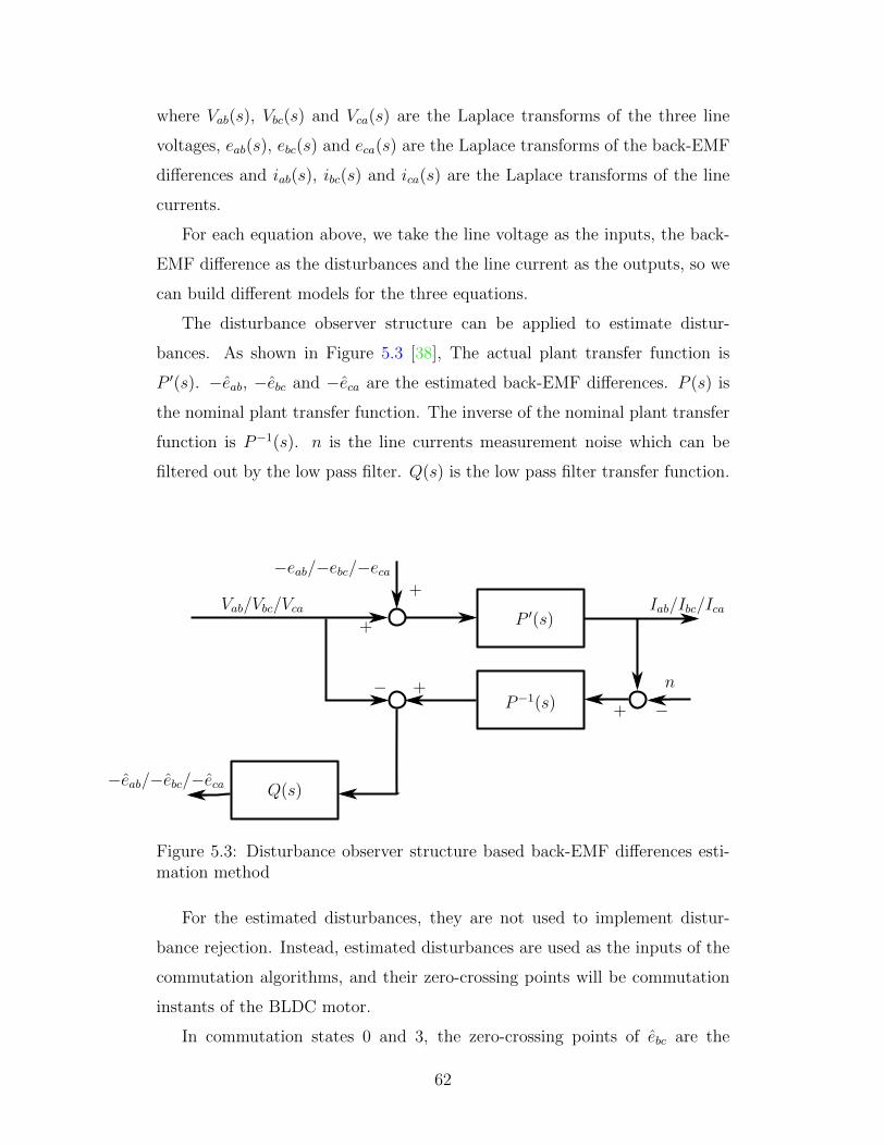
where Vab(s), Vbc(s) and Vca(s) are the Laplace transforms of the three line

voltages, eab(s), ebc(s) and eca(s) are the Laplace transforms of the back-EMF

differences and iab(s), ibc(s) and ica(s) are the Laplace transforms of the line

currents.

For each equation above, we take the line voltage as the inputs, the back-

EMF difference as the disturbances and the line current as the outputs, so we

can build different models for the three equations.

The disturbance observer structure can be applied to estimate distur-

bances. As shown in Figure 5.3 [38], The actual plant transfer function is

P ′(s). −eab, −ebc and −eca are the estimated back-EMF differences. P (s) is

the nominal plant transfer function. The inverse of the nominal plant transfer

function is P−1(s). n is the line currents measurement noise which can be

filtered out by the low pass filter. Q(s) is the low pass filter transfer function.

Vab/Vbc/Vca

−eab/−ebc/−eca

P ′(s)

P−1(s)

Iab/Ibc/Ica

n

Q(s)

+

+

+ −+−

−eab/−ebc/−eca

Figure 5.3: Disturbance observer structure based back-EMF differences esti-mation method

For the estimated disturbances, they are not used to implement distur-

bance rejection. Instead, estimated disturbances are used as the inputs of the

commutation algorithms, and their zero-crossing points will be commutation

instants of the BLDC motor.

In commutation states 0 and 3, the zero-crossing points of ebc are the

62

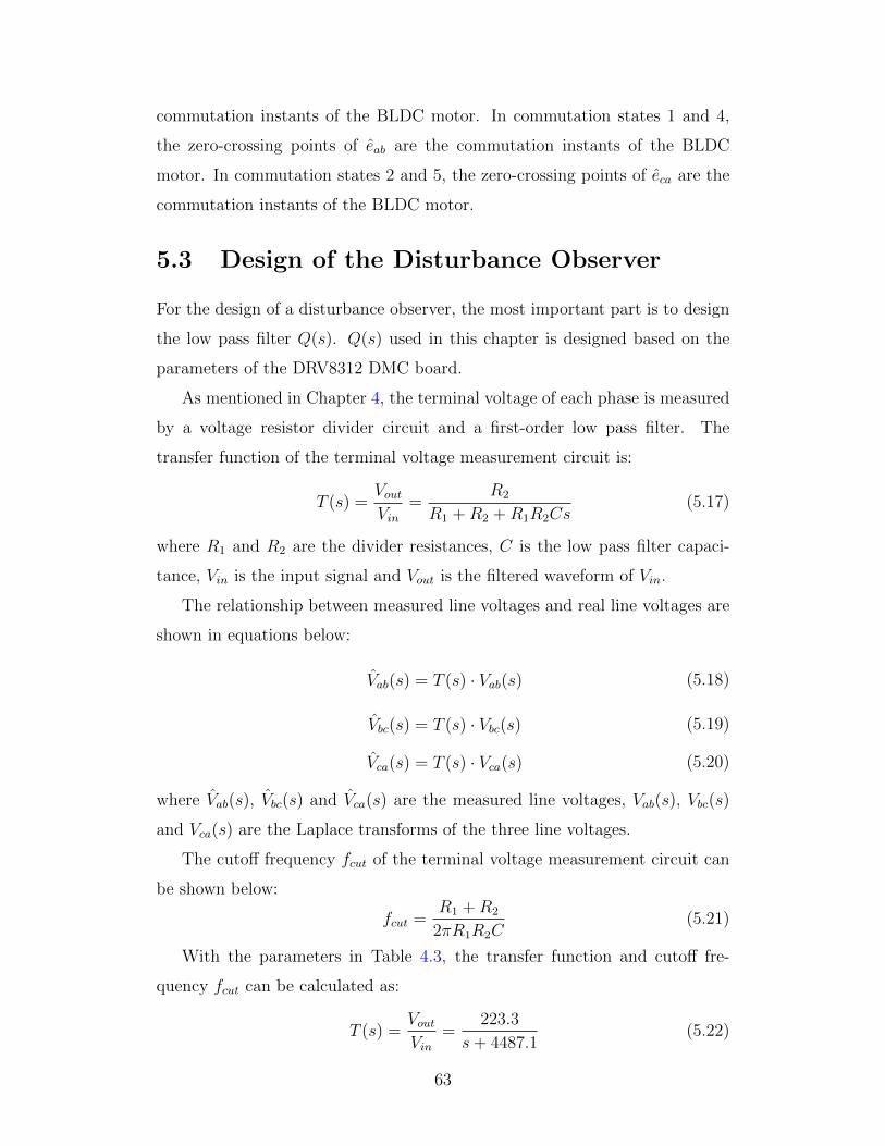
commutation instants of the BLDC motor. In commutation states 1 and 4,

the zero-crossing points of eab are the commutation instants of the BLDC

motor. In commutation states 2 and 5, the zero-crossing points of eca are the

commutation instants of the BLDC motor.

5.3 Design of the Disturbance Observer

For the design of a disturbance observer, the most important part is to design

the low pass filter Q(s). Q(s) used in this chapter is designed based on the

parameters of the DRV8312 DMC board.

As mentioned in Chapter 4, the terminal voltage of each phase is measured

by a voltage resistor divider circuit and a first-order low pass filter. The

transfer function of the terminal voltage measurement circuit is:

T (s) =VoutVin

=R2

R1 +R2 +R1R2Cs(5.17)

where R1 and R2 are the divider resistances, C is the low pass filter capaci-

tance, Vin is the input signal and Vout is the filtered waveform of Vin.

The relationship between measured line voltages and real line voltages are

shown in equations below:

Vab(s) = T (s) · Vab(s) (5.18)

Vbc(s) = T (s) · Vbc(s) (5.19)

Vca(s) = T (s) · Vca(s) (5.20)

where Vab(s), Vbc(s) and Vca(s) are the measured line voltages, Vab(s), Vbc(s)

and Vca(s) are the Laplace transforms of the three line voltages.

The cutoff frequency fcut of the terminal voltage measurement circuit can

be shown below:

fcut =R1 +R2

2πR1R2C(5.21)

With the parameters in Table 4.3, the transfer function and cutoff fre-

quency fcut can be calculated as:

T (s) =VoutVin

=223.3

s+ 4487.1(5.22)

63

fcut = 714.2 Hz (5.23)

The low pass filter Q(s) is designed to be the same as the transfer function

of the terminal voltage measurement circuit.

Q(s) = T (s) =223.3

s+ 4487.1(5.24)

For the measurement of three phase currents, three differential amplifier

circuits are used to measure three phase currents. The per unit range of -

1.0 to 1.0 is corresponding to the real current from −8.65 A to 8.65 A. The

relationship can be shown in equations below:

Iab(s) = K · Iab (5.25)

Ibc(s) = K · Ibc (5.26)

Ica(s) = K · Ica (5.27)

K = 8.65 A (5.28)

where iab(s), ibc(s) and ica(s) represent line currents. Iab, Ibc and Ica are per

unit line currents.

Vab/Vbc/Vca

−eab/−ebc/−eca

uP ′(s)

KP−1(s)

Iab/Ibc/Ica

n

Q(s)

+

+

++−

−eab/−ebc/−eca

T−1(s)

T−1(s)

T−1(s)

K−1

−

Figure 5.4: Modified disturbance observer structure considering voltage andcurrent sensing circuits

The modified disturbance observer structure is shown in Figure 5.4 [38].

The estimated back-EMF differences −eab, −ebc and −eca can be shown as

64

[38]:

−eab = −Vab · T−1(s) ·Q(s) +K · P−1(s) ·Q(s) · (Iab − n) (5.29)

−ebc = −Vbc · T−1(s) ·Q(s) +K · P−1(s) ·Q(s) · (Ibc − n) (5.30)

−eca = −Vca · T−1(s) ·Q(s) +K · P−1(s) ·Q(s) · (Ica − n) (5.31)

The per unit line currents Iab, Ibc and Ica can be shown as:

Iab = [Vab · T−1(s)− eab] · P ′(s) ·K−1 (5.32)

Ibc = [Vbc · T−1(s)− ebc] · P ′(s) ·K−1 (5.33)

Ica = [Vca · T−1(s)− eca] · P ′(s) ·K−1 (5.34)

Then −eab, −ebc and −eca can be modified as [38]:

−eab = −Vab · T−1(s) ·Q(s) + P−1(s) · P ′(s) · Vab · T−1(s) ·Q(s)

+ [−P−1(s) · P ′(s) · eab − nKP−1(s)] ·Q(s)(5.35)

−ebc = −Vbc · T−1(s) ·Q(s) + P−1(s) · P ′(s) · Vbc · T−1(s) ·Q(s)

+ [−P−1(s) · P ′(s) · ebc − nKP−1(s)] ·Q(s)(5.36)

−eca = −Vca · T−1(s) ·Q(s) + P−1(s) · P ′(s) · Vca · T−1(s) ·Q(s)

+ [−P−1(s) · P ′(s) · eca − nKP−1(s)] ·Q(s)(5.37)

If there is no modeling error, P ′(s) and P (s) are equal as:

P ′(s) = P (s) =1

Ls+R(5.38)

where R is the phase stator resistance and L is the phase stator inductance.

The low pass filter can filter out the measurement noise n. Then, −eab,

−ebc and −eca can be simplified as [38]:

−eab = −eab ·Q(s) (5.39)

−ebc = −ebc ·Q(s) (5.40)

−eca = −eca ·Q(s) (5.41)

65

Thus, the modified disturbance observer structure can be applied to esti-

mate the back-EMF differences:

eab = Vab −K · P−1(s) ·Q(s) · Iab

ebc = Vbc −K · P−1(s) ·Q(s) · Ibc

eca = Vca −K · P−1(s) ·Q(s) · Ica

(5.42)

5.4 Phase Delay Compensation

Although the sensorless control method based on the disturbance observer

does not require a 30 electrical degree shift, phase delay will be introduced

because of low pass filters applied in the designed disturbance observer struc-

ture. Figure 5.5 shows the waveforms of the real back-EMF differences and

the estimated back-EMF differences at a speed of 1000 r/min. From the sim-

ulation results, we can see that the estimated back-EMF differences lag the

real back-EMF differences. Figure 5.6 shows the condition at a speed of 2000

r/min. Compared with Figure 5.5, we can see that the phase delay becomes

larger at a higher speed.

Ideally, the zero-crossing points of back-EMF differences can be treated

as the commutation instants of a BLDC motor. But due to the phase delay

introduced by low pass filters, phase delay compensation should be done to

ensure the correct commutation instants.

Based on the BLDC motor electrical period, the phase delay introduced

by low pass filters can be calculated as:

θ = tan−1(R1 ·R2 · C · ωe

R1 +R2

)

= tan−1(R1 ·R2 · CR1 +R2

· 2π

T)

(5.43)

where θ is the phase delay, T is one electrical period, R1 and R2 are the divider

resistances and C is the low pass filter capacitance.

For each of the six commutation states, one back-EMF difference is chosen

to identify the commutation instant. The back-EMF difference will start from

a maximum positive value or a minimum negative value, then it will reach the

66

0.6 0.605 0.61 0.615 0.62−0.5

0

0.5

1

time (s)

Voltage (V

) eabeab

0.6 0.605 0.61 0.615 0.62−0.5

0

0.5

1

time (s)

Voltage

(V)

ebcebc

0.6 0.605 0.61 0.615 0.62−0.5

0

0.5

1

time (s)

Voltage (V

)

ecaeca

Figure 5.5: Simulation results of the estimated back-EMF differences and thereal back-EMF differences at 1000 rpm with 0.04 Nm load

zero-crossing point. Theoretically, the back-EMF difference shape is trape-

zoidal, so we can assume that each chosen back-EMF difference varies linearly

with electrical angle during its commutation state.

To compensate the phase delay, threshold values ,which trigger commu-

tation instants, should be set based on the calculated phase delay instead of

zero [38]. With the similar triangles formula, the threshold values used in the

chapter to compensate the phase delay can be calculated as [38]:

Vp =θ

60· Vpmax (5.44)

Vn =θ

60· Vpmin (5.45)

where Vp is the threshold value when the back-EMF difference varies from the

maximum positive value to zero, Vn is the threshold value when the back-EMF

difference varies from the minimum negative value to zero, θ is the calculated

67

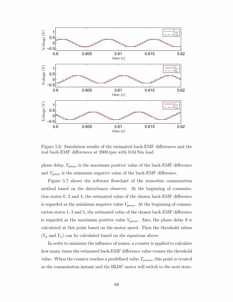
0.6 0.605 0.61 0.615 0.62−0.5

00.5

1

time (s)

Voltag

e (V

) eabeab

0.6 0.605 0.61 0.615 0.62−0.5

00.5

1

time (s)

Voltag

e (V

)

ebcebc

0.6 0.605 0.61 0.615 0.62−0.5

00.5

1

time (s)

Voltage

(V)

ecaeca

Figure 5.6: Simulation results of the estimated back-EMF differences and thereal back-EMF differences at 2000 rpm with 0.04 Nm load

phase delay, Vpmax is the maximum positive value of the back-EMF difference

and Vpmin is the minimum negative value of the back-EMF difference.

Figure 5.7 shows the software flowchart of the sensorless commutation

method based on the disturbance observer. At the beginning of commuta-

tion states 0, 2 and 4, the estimated value of the chosen back-EMF difference

is regarded as the minimum negative value Vpmin. At the beginning of commu-

tation states 1, 3 and 5, the estimated value of the chosen back-EMF difference

is regarded as the maximum positive value Vpmax. Also, the phase delay θ is

calculated at this point based on the motor speed. Then the threshold values

(Vp and Vn) can be calculated based on the equations above.

In order to minimize the influence of noises, a counter is applied to calculate

how many times the estimated back-EMF difference value crosses the threshold

value. When the counter reaches a predefined value Tnoises, this point is treated

as the commutation instant and the BLDC motor will switch to the next state.

68

Dis

turb

ance

Ife b

c<Vn

Tim

eco

unte

r++

Ifti

me

counte

r<Tnoises

Com

muta

tion

inst

ants

Yes

No

Ifst

ate=

0

Ife a

b>Vp

Ifst

ate=

1

Ife c

a<Vn

Ifst

ate=

2

Ife b

c>Vp

Ifst

ate=

3

Ife a

b<Vn

Ifst

ate=

4

Ife c

a>Vp

Ifst

ate=

5

No

No

No

No

No

No

Yes

Yes

Yes

Yes

Yes

Yes

Cal

cula

teVn

Cal

cula

teVp

Cal

cula

teVn

Cal

cula

teVn

Cal

cula

teVp

Cal

cula

teVp

obse

rver

Dis

turb

ance

obse

rver

Dis

turb

ance

obse

rver

Dis

turb

ance

obse

rver

Dis

turb

ance

obse

rver

Dis

turb

ance

obse

rver

e bc

e ab

e ca

e bc

e ab

e ca

Fig

ure

5.7:

Sof

twar

eflow

char

tof

the

senso

rles

sco

mm

uta

tion

met

hod

bas

edon

the

dis

turb

ance

obse

rver

stru

cture

69

5.5 Proposed Sensorless Drive

Figure 5.8 shows the proposed sensorless drive for speed control of a BLDC

motor. A proportional integral (PI) controller is applied to determine the duty

cycle of the PWM signals based on the difference between the measured motor

speed ω and the reference motor speed ω∗.

The measured three phase currents and the three phase terminal voltages

are the inputs of the disturbance observer. The estimated back-EMF differ-

ences eab, ebc and eca together with the measured motor speed are the inputs

of the commutation trigger block. The commutation sequence of the proposed

method is shown in Table 5.1.

Because the proposed method is based on back-EMF differences, a starting

procedure is required to speed up the BLDC motor to a higher speed. In this

chapter, the conventional open-loop starting method, as described in Chapter

4, is applied to blindly start the BLDC motor.

Commutation States Commutation Instants

0 ebc = Vn1 eab = Vp2 eca = Vn3 ebc = Vp4 eab = Vn5 eca = Vp

Table 5.1: Commutation sequence for the method based on disturbance ob-server

5.6 Experimental Results

In this section, we present the experiment results of the proposed sensorless

BLDC motor drive based on the disturbance observer structure at different

speeds. Compensation of the phase delay introduced by the disturbance ob-

server structure is also discussed.

70

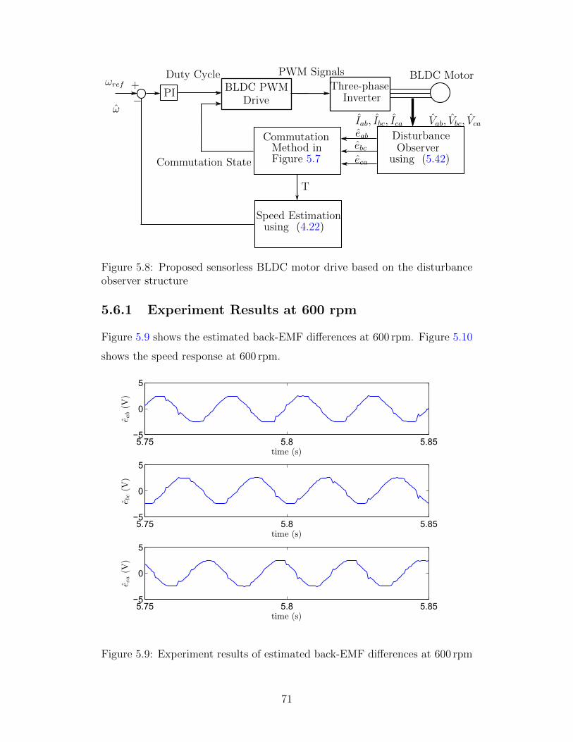
Three-phaseInverter

Disturbanceeabebceca

T

Speed Estimationusing (4.22)

−PI

ωref

ω

+Duty Cycle BLDC Motor

Commutation State

Vab, Vbc, VcaIab, Ibc, Ica

CommutationMethod inFigure 5.7

BLDC PWMDrive

PWM Signals

Observerusing (5.42)

Figure 5.8: Proposed sensorless BLDC motor drive based on the disturbanceobserver structure

5.6.1 Experiment Results at 600 rpm

Figure 5.9 shows the estimated back-EMF differences at 600 rpm. Figure 5.10

shows the speed response at 600 rpm.

5.75 5.8 5.85−5

0

5

time (s)

eab(V

)

5.75 5.8 5.85−5

0

5

time (s)

ebc(V

)

5.75 5.8 5.85−5

0

5

time (s)

eca(V

)

Figure 5.9: Experiment results of estimated back-EMF differences at 600 rpm

71

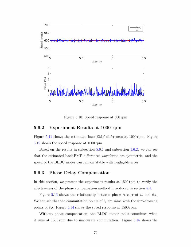
5 5.5 6 6.5500

550

600

650

700

time (s)

Speed(rpm)

5 5.5 6 6.5

0

1

2

3

4

5

time (s)

Error(%

)

ωref

ω

Figure 5.10: Speed response at 600 rpm

5.6.2 Experiment Results at 1000 rpm

Figure 5.11 shows the estimated back-EMF differences at 1000 rpm. Figure

5.12 shows the speed response at 1000 rpm.

Based on the results in subsection 5.6.1 and subsection 5.6.2, we can see

that the estimated back-EMF differences waveforms are symmetric, and the

speed of the BLDC motor can remain stable with negligible error.

5.6.3 Phase Delay Compensation

In this section, we present the experiment results at 1500 rpm to verify the

effectiveness of the phase compensation method introduced in section 5.4.

Figure 5.13 shows the relationship between phase A current ia and eab.

We can see that the commutation points of ia are same with the zero-crossing

points of eab. Figure 5.14 shows the speed response at 1500 rpm.

Without phase compensation, the BLDC motor stalls sometimes when

it runs at 1500 rpm due to inaccurate commutation. Figure 5.15 shows the

72

10.9 10.91 10.92 10.93 10.94 10.95 10.96−5

0

5

time (s)

eab(V

)

10.9 10.91 10.92 10.93 10.94 10.95 10.96−5

0

5

time (s)

ebc(V

)

10.9 10.91 10.92 10.93 10.94 10.95 10.96−5

0

5

time (s)

eca(V

)

Figure 5.11: Experiment results of estimated back-EMF differences at1000 rpm

10 10.5 11 11.5900

950

1000

1050

1100

time (s)

Speed(rpm)

10 10.5 11 11.5

0

1

2

3

4

5

time (s)

Error(%

)

ωref

ω

Figure 5.12: Speed response at 1000 rpm

73

10.88 10.885 10.89 10.895 10.9−10

−5

0

5

10

eab(V

)

time (s)10.88 10.885 10.89 10.895 10.9

−1

0

1

ia(A

)

Figure 5.13: Phase A current and eab at 1500 rpm

10 10.5 11 11.51400

1450

1500

1550

1600

time (s)

Speed(rpm)

10 10.5 11 11.5

0

1

2

3

4

5

time (s)

Error(%

)

ωref

ω

Figure 5.14: Speed response at 1500 rpm

74

0.015 0.02 0.025 0.03 0.035 0.04−1

0

1

Estim

atedsignal(V

)

time (s)

Before compensation

0.015 0.02 0.025 0.03 0.035 0.040

2

4

Idealsignal(V

)

0.015 0.02 0.025 0.03 0.035 0.04−1

0

1

Estim

atedsignal(V

)

time (s)

Before compensation

0.015 0.02 0.025 0.03 0.035 0.040

2

4

Idealsignal(V

)

Figure 5.15: Ideal commutation signal and estimated commutation signal at1500 rpm

experiment results of the relationship between the ideal commutation signal

(Hall-effect sensor A output) and the estimated commutation signal (virtual

Hall-effect sensor A output obtained from the sensorless commutation method)

at 1500 rpm.

From Figure 5.15, we can see that the estimated commutation signal matches

well with the ideal commutation signal with phase compensation. For high

speed applications, it is necessary to compensate the phase delay caused by

the disturbance observer structure [38].

With phase compensation method, the sensorless commutation method can

get accurate commutation points, and the high speed range can be expanded.

75

5.7 Comparison with the Sensorless Drive based

on Line Voltage Differences

In this section, we make a comparison of the proposed sensorless BLDC motor

drive based on the disturbance observer structure and the sensorless drive

introduced in Chapter 4.

Based on the analysis above, both of these two sensorless drives can achieve

precise sensorless commutation. However, they all need compensation for the

phase delay caused by the low pass filter. The electrical frequency of the motor

must be smaller than the cutoff frequency fcut of the low pass filter, which is

714.2 Hz.

For the sensorless drive based on the line voltage differences, the maximum

allowable phase delay from the low pass filter is 30 (electrical frequency equals

412.5 Hz). In contrast, the maximum allowable phase delay is 60 (electrical

frequency equals 1237.4 Hz) for the sensorless BLDC motor drive based on the

disturbance observer structure. For the given motor drive board, we can see

that disturbance observer based sensorless drive allows the electrical frequency

of the motor to be up to the cutoff frequency of the low pass filter. Disturbance

observer based sensorless drive has a wider high speed range in comparison

with the sensorless drive based on the line voltage differences.

Both of these two sensorless drives are based on back-EMFs, so they all

have poor performance in the low speed range. Figure 5.16 shows Vabca and

eab waveforms at low speeds. We can see that the waveforms are distorted,

and we can not get accurate commutation points with either of the proposed

sensorless drives.

Figure 5.17 and Figure 5.18 show the simulation results of the speed re-

sponse at low speed (500 rpm) and high speed (1500 rpm) during loading tran-

sient, respectively. For 500 rpm, a step load (0.05 Nm) is applied at 0.3 s.

For 1500 rpm, a step load (0.05 Nm) is applied at 0.5 s. From the simulation

results, we can see that the speed response of the two sensorless drives are

similar. For both low and high speeds conditions, the motor speed decreases

after applying the load, and then it will keep on tracking the reference speed

76

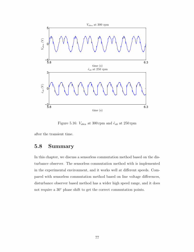
5.8 6.3−5

0

5

time (s)

Vabca(V

)

Vabca at 300 rpm

5.8 6.3−3

0

3

time (s)

eab(V

)

eab at 250 rpm

Figure 5.16: Vabca at 300 rpm and eab at 250 rpm

after the transient time.

5.8 Summary

In this chapter, we discuss a sensorless commutation method based on the dis-

turbance observer. The sensorless commutation method with is implemented

in the experimental environment, and it works well at different speeds. Com-

pared with sensorless commutation method based on line voltage differences,

disturbance observer based method has a wider high speed range, and it does

not require a 30 phase shift to get the correct commutation points.

77

0 0.1 0.2 0.3 0.4 0.50

500

1000

1500

Speed(rpm)

Speed response (line voltage differences)

0 0.1 0.2 0.3 0.4 0.50

500

1000

1500

time (s)

Speed(rpm)

time(s)Speed response (disturbance observer)

Figure 5.17: Speed response at 500 rpm during loading transient

0 0.2 0.4 0.6 0.8 10

1000

2000

3000

Speed(rpm)

Speed response (line voltage differences)

0 0.2 0.4 0.6 0.8 10

1000

2000

3000

time (s)

Speed(rpm)

time(s)Speed response (disturbance observer)

Figure 5.18: Speed response at 1500 rpm during loading transient

78

Chapter 6

Conclusions

6.1 Summary of Research

This thesis focuses on the implementation of two sensorless control techniques

for a BLDC motor. Firstly, we discuss a sensorless control method, which uti-

lizes line voltage differences to estimate the zero-crossing points of back-EMFs.

The line voltage differences have the same zero-crossing points as back-EMFs,

which are verified by the simulation results. This method only requires three

motor terminal voltages without the need for the motor neutral voltage. This

sensorless control method is also implemented in the experimental environ-

ment, and a compensation method is applied to compensate the phase delay

introduced by the the low-pass filters in the terminal voltage sensing circuits.

Then we introduce a back-EMF differences based sensorless control method,

which does not require any phase shift to get the commutation instants. The

disturbance observer structure is applied to estimate the back-EMF differences.

Simulation results show that the estimated back-EMF differences matches well

with the real back-EMF differences except for a phase delay caused by the

low pass filter in the disturbance observer structure. This sensorless control

method with phase delay compensation is implemented in the experimental

environment.

From the experiment results, we conclude that both of these two sensorless

control techniques can be applied in commutating a BLDC motor. Phase delay

compensation methods are necessary for high speed operation. Disturbance

observer based method has a better high speed capability. Because both of

79

these two sensorless control techniques are based on back-EMFs, they have

limiting low speed capability. Based on the Simulink simulation results, both

of these two sensorless drives are able to work well even with load disturbance.

6.2 Future Work

In the past few decades, fuzzy logic controllers gained wide attentions and have

been applied in BLDC motor drives [32][34]. Fuzzy controller-based BLDC

motor drive has a better performance for the varying operating conditions of

the motor, such as motor parameters variation and load uncertainties [34].

For the future work, we will apply the fuzzy logic controller in the speed

control loop, together with the sensorless commutation techniques investigated

in this thesis, to build a combined BLDC sensorless control drive with better

performance.

80

Bibliography

[1] R. Becerra, T. Jahns, and M. Ehsani. Four-quadrant sensorless brushless

ecm drive. In Applied Power Electronics Conference and Exposition, 1991.

APEC’91. Conference Proceedings, 1991., Sixth Annual, pages 202–209.

IEEE, 1991.

[2] M. Bonfe and M. Bergo. A brushless motor drive with sensorless control

for commercial vehicle hydraulic pumps. In 2008 IEEE International

Symposium on Industrial Electronics, pages 612–617. IEEE, 2008.

[3] C. W. Brokish. Emulation fundamentals for tis dsp solutions. Texas

Instruments Application Report SPRA439C, 2005.

[4] C.-H. Chen and M.-Y. Cheng. A new sensorless commutation drive for

brushless dc motors and alternators. In 2006 IEEE International Sympo-

sium on Industrial Electronics, volume 3, pages 2116–2121. IEEE, 2006.

[5] W.-H. Chen, J. Yang, L. Guo, and S. Li. Disturbance-observer-based

control and related methodsan overview. IEEE Transactions on Industrial

Electronics, 63(2):1083–1095, 2016.

[6] P. Damodharan and K. Vasudevan. Sensorless brushless dc motor drive

based on the zero-crossing detection of back electromotive force (emf)

from the line voltage difference. IEEE Transactions on Energy Conver-

sion, 25(3):661–668, 2010.

[7] A. Deenadayalan, C. Dhananjai, and G. S. Ilango. Modified sliding mode

observer for wide speed range operation of brushless dc motor. Frontiers

of Electrical and Electronic Engineering, 7(4):467–476, 2012.

81

[8] J. C. Gamazo-Real, E. Vazquez-Sanchez, and J. Gomez-Gil. Position

and speed control of brushless dc motors using sensorless techniques and

application trends. Sensors, 10(7):6901–6947, 2010.

[9] A. Girolkar and G. Bhuvaneswari. Control of pmbldc motor using third

harmonic back emf sensing with zigzag transformer. In Electrical Energy

Systems (ICEES), 2014 IEEE 2nd International Conference on, pages

110–115. IEEE, 2014.

[10] D. C. Hanselman. Brushless permanent magnet motor design. The Writ-

ers’ Collective, 2003.

[11] F. Hicham, D. Mohamed, R. Abdellatif, and B. Pierre. Sliding mode

observer for position and speed estimations in brushless dc motor (bldcm).

In Industrial Technology, 2004. IEEE ICIT’04. 2004 IEEE International

Conference on, volume 1, pages 121–126. IEEE, 2004.

[12] T. Hurd and I. Sever. Hardware-controlled brushless dc motors ease the

burden on cpus. EDN (Electrical Design News), 55(16):24, 2010.

[13] K. Iizuka, H. Uzuhashi, M. Kano, T. Endo, and K. Mohri. Microcomputer

control for sensorless brushless motor. IEEE Transactions on Industry

Applications, (3):595–601, 1985.

[14] M. Ikhlas. Rotor Position Identification for Brushless DC motor. PhD

thesis, The University of Western Ontario, 2015.

[15] T. Instruments. Drv83x2 three-phase pwm motor driver, december 2014.

URL http://www. ti. com/lit/ds/symlink/drv8332. pdf. Rev: SLES256E–

May, 2010.

[16] T. Instruments. Drv8312-c2-kit hardware reference guide. C2000 &

DRV8312 Systems and Applications Team, Apr, 2011.

[17] T. Instruments. Tms320x2802x, 2803x piccolo analog to digital converter

(adc) and comparator. Reference Guide, Dec, 2011.

82

[18] T. Instruments. Tms320x2802x, 2803x piccolo enhanced pulse width mod-

ulator (epwm) module. Reference Guide, Mar, 2011.

[19] T. Kim, C. Kim, and J. Lyou. A new sensorless drive scheme for a bldc

motor based on the terminal voltage difference. In IECON 2011-37th

Annual Conference on IEEE Industrial Electronics Society, pages 1710–

1715. IEEE, 2011.

[20] T. Kim, H. Lee, and M. Ehsani. Position sensorless brushless dc mo-

tor/generator drives: review and future trends. IET Electric Power Ap-

plications, 1(4):557–564, 2007.

[21] T.-H. Kim, H.-W. Lee, and M. Ehsani. State of the art and future trends

in position sensorless brushless dc motor/generator drives. In 31st Annual

Conference of IEEE Industrial Electronics Society, 2005. IECON 2005.,

pages 8–pp. IEEE, 2005.

[22] T.-S. Kim, B.-G. Park, D.-M. Lee, J.-S. Ryu, and D.-S. Hyun. A new ap-

proach to sensorless control method for brushless dc motors. International

Journal of Control, Automation, and Systems, 6(4):477–487, 2008.

[23] R. Krishnan. Permanent magnet synchronous and brushless DC motor

drives. CRC press, 2009.

[24] Y.-S. Lai and Y.-K. Lin. Novel back-emf detection technique of brushless

dc motor drives for wide range control without using current and position

sensors. IEEE Transactions on power electronics, 23(2):934–940, 2008.

[25] Y.-S. Lai, F.-S. Shyu, and Y.-H. Chang. Novel loss reduction pulsewidth

modulation technique for brushless dc motor drives fed by mosfet inverter.

IEEE transactions on power electronics, 19(6):1646–1652, 2004.

[26] Z. Li, S. Cheng, Y. Qin, and K. Cai. A novel line-to-line back emf calcu-

lation for sensorless brushless dc motor drives. In Electrical Machines and

Systems, 2008. ICEMS 2008. International Conference on, pages 1406–

1411. IEEE, 2008.

83

[27] P. Madaan. Brushless dc motors–part i: Construction and operating

principles. Cypress Semiconductor, 11, 2013.

[28] L. Mingyao, Z. Zhiyao, and L. Keman. A novel and easy-realizing initial

rotor position detection method and speedup algorithm for sensorless bldc

motor drives. ICEMS 2008, pages 2860–2865, 2008.

[29] J. C. Moreira. Indirect sensing for rotor flux position of permanent magnet

ac motors operating over a wide speed range. IEEE Transactions on

Industry Applications, 32(6):1394–1401, 1996.

[30] M. Mubeen. Brushless dc motor primer. Motion Tech Trends, 2008.

[31] S. Ogasawara and H. Akagi. An approach to position sensorless drive

for brushless dc motors. IEEE Transactions on Industry Applications,

27(5):928–933, 1991.

[32] A. Rubaai, D. Ricketts, and M. D. Kankam. Laboratory implementation

of a microprocessor-based fuzzy logic tracking controller for motion con-

trols and drives. IEEE Transactions on Industry Applications, 38(2):448–

456, 2002.

[33] E. Schrijver and J. Van Dijk. Disturbance observers for rigid mechanical

systems: equivalence, stability, and design. Journal of Dynamic Systems,

Measurement, and Control, 124(4):539–548, 2002.

[34] R. Shanmugasundram, K. M. Zakariah, and N. Yadaiah. Implementation

and performance analysis of digital controllers for brushless dc motor

drives. IEEE/ASME transactions on mechatronics, 19(1):213–224, 2014.

[35] J. Shao. An improved microcontroller-based sensorless brushless dc (bldc)

motor drive for automotive applications. IEEE Transactions on industry

applications, 42(5):1216–1221, 2006.

[36] J. Shao, D. Nolan, and T. Hopkins. A novel direct back emf detection for

sensorless brushless dc (bldc) motor drives. In Applied Power Electronics

84

Conference and Exposition, 2002. APEC 2002. Seventeenth Annual IEEE,

volume 1, pages 33–37. IEEE, 2002.

[37] B. Terzic and M. Jadric. Design and implementation of the extended

kalman filter for the speed and rotor position estimation of brushless dc

motor. IEEE Transactions on Industrial Electronics, 48(6):1065–1073,

2001.

[38] S. Wang and A.-C. Lee. A 12-step sensorless drive for brushless dc motors

based on back-emf differences. IEEE Transactions on Energy Conversion,

30(2):646–654, 2015.

[39] S. Wang, C.-H. Lu, and A.-C. Lee. Disturbance observer structure ap-

plied to sensorless brushless dc motors drive. International Journal of

Computer Theory and Engineering, 7(2):92, 2015.

[40] P. Yedamale. Brushless dc (bldc) motor fundamentals. Microchip Tech-

nology Inc, 20:3–15, 2003.

85