A Study of Stellar Model with Kramer’s Opacity by Using ... · DOI: 10.4236/ijaa.2017.73015 Sep. 11, 2017 185 International Journal of Astronomy and Astrophysics A Study of Stellar

International Journal of Astronomy and Astrophysics, 2017, 7, 185-201 http://www.scirp.org/journal/ijaa

ISSN Online: 2161-4725 ISSN Print: 2161-4717

DOI: 10.4236/ijaa.2017.73015 Sep. 11, 2017 185 International Journal of Astronomy and Astrophysics

A Study of Stellar Model with Kramer’s Opacity by Using Runge Kutta Method with Programming C

Md. Abdullah Bin Masud*, Shammi Akter Doly

Department of Computer Science & Engineering, Shanto-Mariam University of Creative Technology, Dhaka, Bangladesh

Abstract In this paper, we have made an investigation on a stellar model with Kramer’s Opacity and negligible abundance of heavy elements. We have determined the structure of a star with mass 2.5M� , i.e. the physical variables like pressure, density, temperature and luminosity at different interior points of the star. We have discussed about some equations of structure, mechanism of energy pro-duction in a star and energy transports in stellar interior in a star and then we have solved radiative envelope and convective core by the matching or fitting point method and Runge-Kutta method by C Programming language. In fu-ture, it will help us to know about the characteristics of new stars.

Keywords Energy Production in Star, Hydrostatic Equilibrium of Star, Mass Conservation, Schwarzschild Method and Variable, Polytropic Core Solution, Packet Solution

1. Introduction

A star is a dense mass that generates its light and heat by nuclear reactions, spe-cifically by the fusion of hydrogen and helium under conditions of enormous temperature and density. Stars are like our sun. The star is powered by hydrogen fusion. The fusion only takes place at core of the star where it is dense enough. The “life” of a star is the time during which it slowly burns up its hydrogen fuel, and evolves only slowly in the process. The star is in force balance between pressure and gravity. It is also in energy balance between production by fusion reactions, transport by photon radiation, and loss from the surface by the (usually) visible radiation by which can detect the star. The “birth” of a star re-fers to the process by which it is formed from diffuse clouds of cold gas that are

How to cite this paper: Masud, M.A.B. and Doly, S.A. (2017) A Study of Stellar Model with Kramer’s Opacity by Using Runge Kutta Method with Programming C. International Journal of Astronomy and Astrophysics, 7, 185-201. https://doi.org/10.4236/ijaa.2017.73015 Received: July 11, 2017 Accepted: September 8, 2017 Published: September 11, 2017 Copyright © 2017 by authors and Scientific Research Publishing Inc. This work is licensed under the Creative Commons Attribution International License (CC BY 4.0). http://creativecommons.org/licenses/by/4.0/

Open Access

http://www.scirp.org/journal/ijaa

https://doi.org/10.4236/ijaa.2017.73015

http://www.scirp.org


http://creativecommons.org/licenses/by/4.0/

M. A. B. Masud, S. A. Doly

DOI: 10.4236/ijaa.2017.73015 186 International Journal of Astronomy and Astrophysics

present in its galaxy [1]. A cloud collapses to form a number of stars when it is disturbed so that its gravity overcomes its motion and pressure. The “death” of a star occurs when its fusion fuel, first hydrogen and then heavier nuclei, have run out. This can be very violent if the star is very massive, ending in things like a black hole and/or a supernova, perhaps leaving a neutron star behind. If the star is not very massive, like the Sun or even smaller, it ends by ejecting part of its atmosphere and then settling down to a cold, dense white dwarf. Harm & Schwarzschild (1955) have shown that the maximal possible mass of the star is 60M� and minimum mass of star is 0.01M� [2]. The chemical element of star is hydrogen, helium and other heavier elements [3]. If hydrogen, helium and other elements are denoted by X, Y and Z respectively, then 1X Y Z+ + = . For the sun X = 0.73, Y = 0.25 and Z = 0.02.

2. HR Diagram

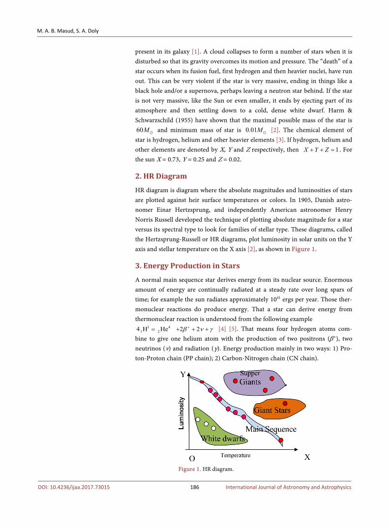
HR diagram is diagram where the absolute magnitudes and luminosities of stars are plotted against heir surface temperatures or colors. In 1905, Danish astro-nomer Einar Hertzsprung, and independently American astronomer Henry Norris Russell developed the technique of plotting absolute magnitude for a star versus its spectral type to look for families of stellar type. These diagrams, called the Hertzsprung-Russell or HR diagrams, plot luminosity in solar units on the Y axis and stellar temperature on the X axis [2], as shown in Figure 1.

3. Energy Production in Stars

A normal main sequence star derives energy from its nuclear source. Enormous amount of energy are continually radiated at a steady rate over long spars of time; for example the sun radiates approximately 1041 ergs per year. Those ther-monuclear reactions do produce energy. That a star can derive energy from thermonuclear reaction is understood from the following example

1 41 24 H He= 2 2β ν γ++ + + [4] [5]. That means four hydrogen atoms com-

bine to give one helium atom with the production of two positrons (β+), two neutrinos (ν) and radiation (γ). Energy production mainly in two ways: 1) Pro-ton-Proton chain (PP chain); 2) Carbon-Nitrogen chain (CN chain).

Figure 1. HR diagram.




4. Hydrostatic Equilibrium of Star

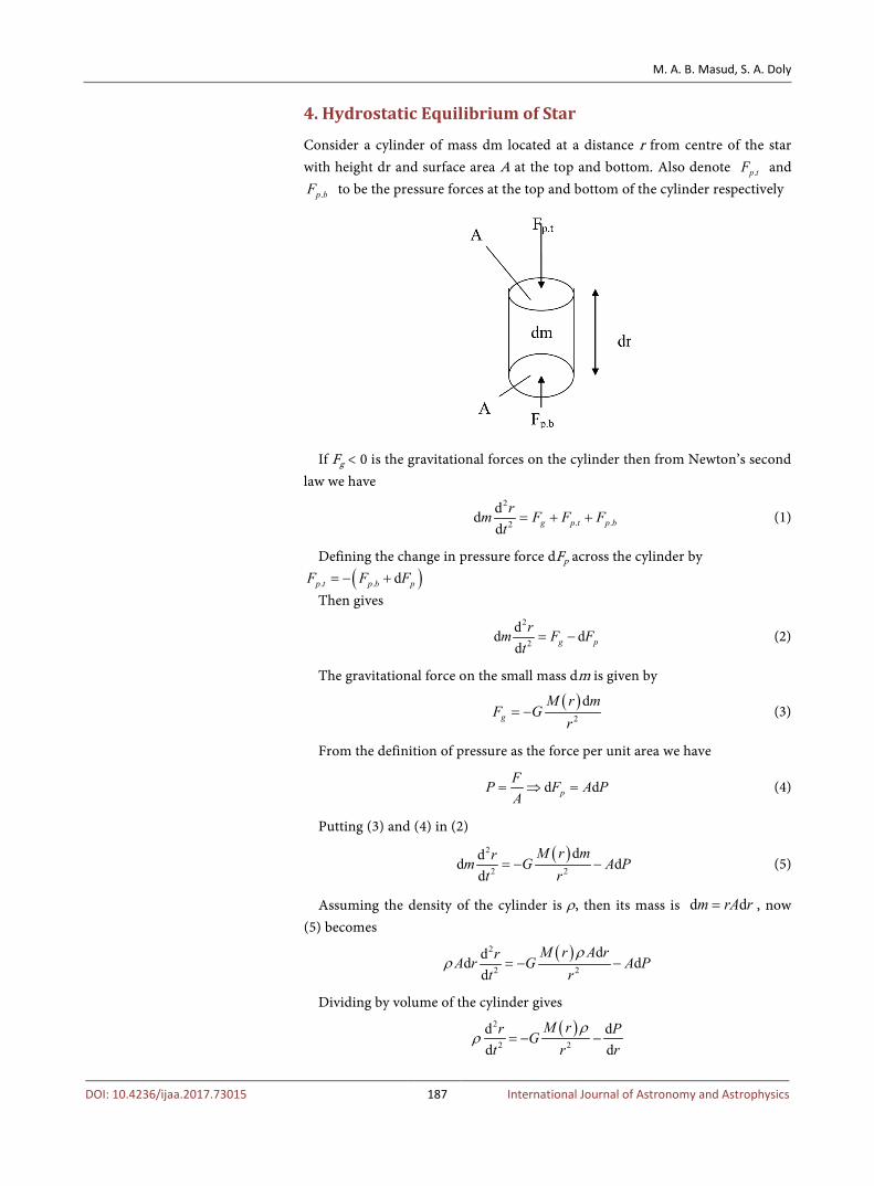
Consider a cylinder of mass dm located at a distance r from centre of the star with height dr and surface area A at the top and bottom. Also denote .p tF and

.p bF to be the pressure forces at the top and bottom of the cylinder respectively

If Fg < 0 is the gravitational forces on the cylinder then from Newton’s second law we have

2

. .2

ddd g p t p b

rm F F Ft

= + + (1)

Defining the change in pressure force dFp across the cylinder by ( ). . dp t p b pF F F= − +

Then gives 2

2

dd dd g p

rm F Ft

= − (2)

The gravitational force on the small mass dm is given by

( )2

dg

M r mF G

r= − (3)

From the definition of pressure as the force per unit area we have

d dpFP F A PA

= ⇒ = (4)

Putting (3) and (4) in (2)

( )2

2 2

ddd dd

M r mrm G A Pt r

= − − (5)

Assuming the density of the cylinder is ρ, then its mass is d dm rA r= , now (5) becomes

( )2

2 2

ddd dd

M r A rrA r G A Pt r

ρρ = − −

Dividing by volume of the cylinder gives

( )2

2 2

d ddd

M rr PGrt r

ρρ = − −




Assuming the star is static the acceleration term will be zero which then leads to

( )2

dd

M rP G gr r

ρρ= − = − (6)

where ( )2

M rg G

r= .

This is the condition of hydrostatic equilibrium.

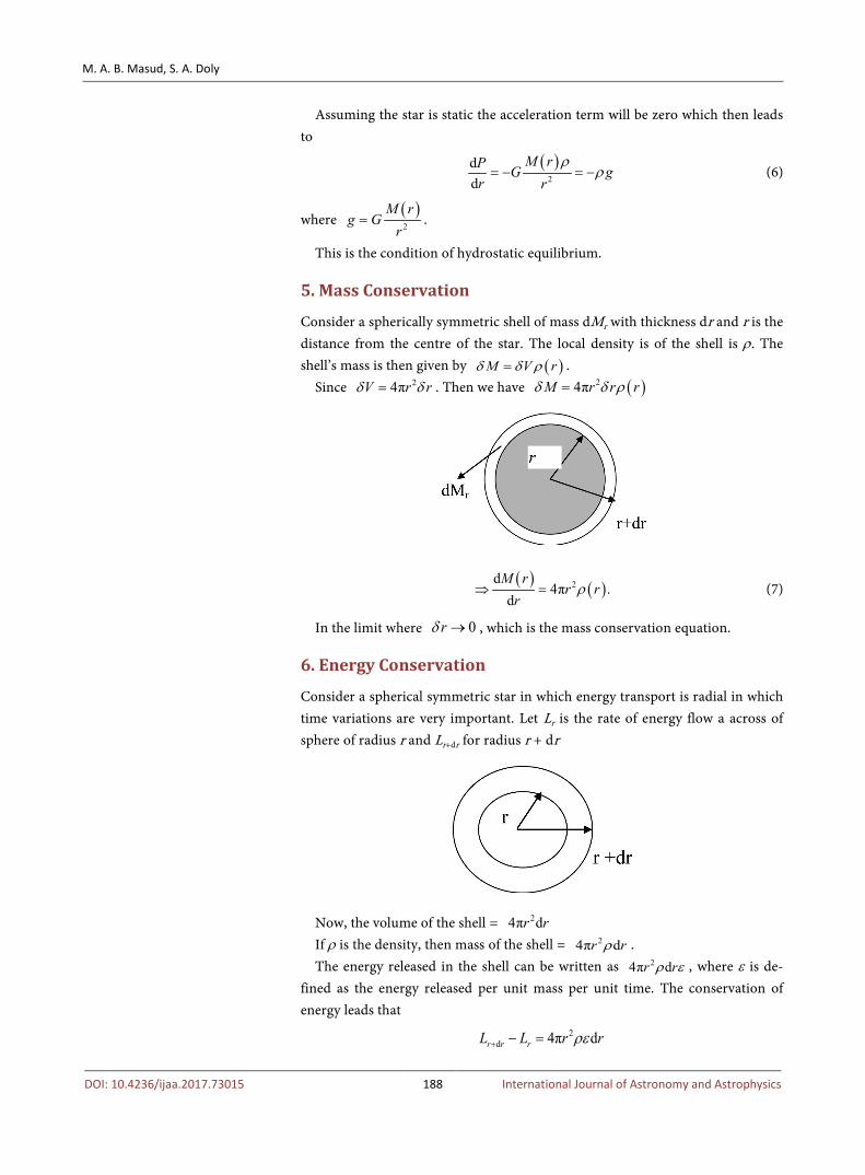
5. Mass Conservation

Consider a spherically symmetric shell of mass dMr with thickness dr and r is the distance from the centre of the star. The local density is of the shell is ρ. The shell’s mass is then given by ( )M V rδ δ ρ= .

Since 24πV r rδ δ= . Then we have ( )24πM r r rδ δ ρ=

( ) ( )2d4π .

dM r

r rr

ρ⇒ = (7)

In the limit where 0rδ → , which is the mass conservation equation.

6. Energy Conservation

Consider a spherical symmetric star in which energy transport is radial in which time variations are very important. Let Lr is the rate of energy flow a across of sphere of radius r and Lr+dr for radius r + dr

Now, the volume of the shell = 24π dr r If ρ is the density, then mass of the shell = 24π dr rρ . The energy released in the shell can be written as 24π dr rρ ε , where ε is de-

fined as the energy released per unit mass per unit time. The conservation of energy leads that

2d 4π dr r rL L r rρε+ − =




2d d 4π ddL r r rr

ρε⇒ ⋅ =

2d 4πdL rr

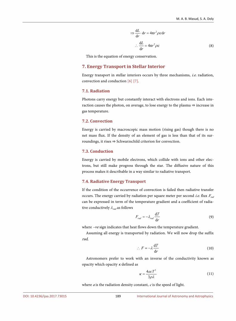
ρε∴ = (8)

This is the equation of energy conservation.

7. Energy Transport in Stellar Interior

Energy transport in stellar interiors occurs by three mechanisms, i.e. radiation, convection and conduction [6] [7].

7.1. Radiation

Photons carry energy but constantly interact with electrons and ions. Each inte-raction causes the photon, on average, to lose energy to the plasma ⇒ increase in gas temperature.

7.2. Convection

Energy is carried by macroscopic mass motion (rising gas) though there is no net mass flux. If the density of an element of gas is less than that of its sur-roundings, it rises ⇒ Schwarzschild criterion for convection.

7.3. Conduction

Energy is carried by mobile electrons, which collide with ions and other elec-trons, but still make progress through the star. The diffusive nature of this process makes it describable in a way similar to radiative transport.

7.4. Radiative Energy Transport

If the condition of the occurrence of convection is failed then radiative transfer occurs. The energy carried by radiation per square meter per second i.e. flux Frad can be expressed in term of the temperature gradient and a coefficient of radia-tive conductively λrad as follows

ddrad radTFr

λ= − (9)

where –ve sign indicates that heat flows down the temperature gradient. Assuming all energy is transported by radiation. We will now drop the suffix

rad,

ddTFr

λ∴ = − (10)

Astronomers prefer to work with an inverse of the conductivity known as opacity which opacity κ defined as

343acTκρλ

= (11)

where a is the radiation density constant, c is the speed of light.




From (11) we have 34

3acTλρκ

= (12)

Putting (12) in (10) we have 34 d

3 dacT TF

rκρ= − (13)

We know flux and luminosity equation is 24πL r F= (14)

2 316 π d3 d

ac r T TLrκρ

⇒ = − [from (13)]

2 3

d 3d 16πT Lr acr T

κρ⇒ = − (15)

This equation is known as the equation of radiative transfer.

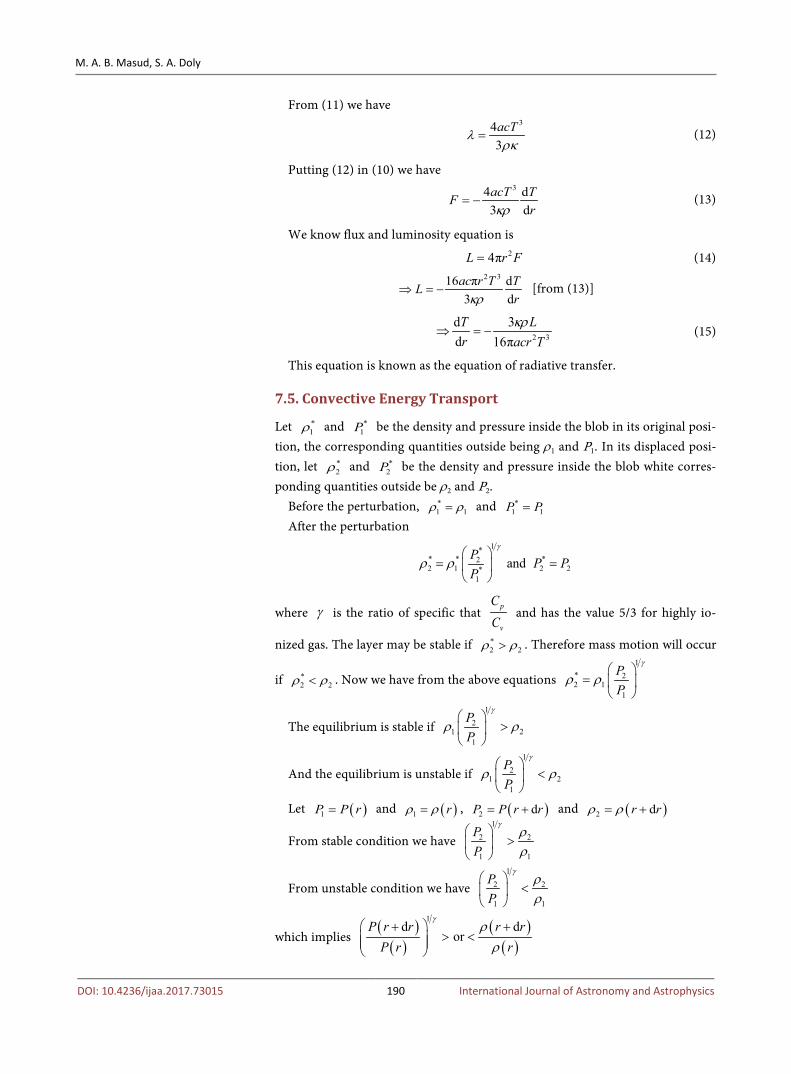
7.5. Convective Energy Transport

Let *1ρ and *

1P be the density and pressure inside the blob in its original posi-tion, the corresponding quantities outside being ρ1 and P1. In its displaced posi-tion, let *

2ρ and *2P be the density and pressure inside the blob white corres-

ponding quantities outside be ρ2 and P2. Before the perturbation, *

1 1ρ ρ= and *1 1P P=

After the perturbation 1*

* * *22 1 2 2*

1

andP P PP

γ

ρ ρ

= =

where γ is the ratio of specific that p

v

CC

and has the value 5/3 for highly io-

nized gas. The layer may be stable if *2 2ρ ρ> . Therefore mass motion will occur

if *2 2ρ ρ< . Now we have from the above equations

1* 22 1

1

PP

γ

ρ ρ

=

The equilibrium is stable if 1

21 2

1

PP

γ

ρ ρ

>

And the equilibrium is unstable if 1

21 2

1

PP

γ

ρ ρ

<

Let ( )1P P r= and ( )1 rρ ρ= , ( )2 dP P r r= + and ( )2 dr rρ ρ= +

From stable condition we have 1

2 2

1 1

PP

γρρ

>

From unstable condition we have 1

2 2

1 1

PP

γρρ

<

which implies ( )( )

( )( )

1d d

orP r r r r

P r r

γρρ

+ +> <




Or 11 d 1 d1 d or 1 d

d dP r r

P r r

γ ρρ

+ > < +

Expanding left side of the above inequalities in Taylor series and neglecting higher order terms we have

1 d 1 d1 d or 1 dd dP r r

P r rρ

λ ρ + > < +

1 d 1 dor

d dP

P r rρ

γ ρ⇒ > <

We know KP THρ

µ=

Taking log and differentiating we have 1 d 1 d 1 d

d d dP T

P r r T rρ

ρ= +

For stability condition we have

1 d 1 d 1 dd d dP P T

P r P r T rγ> −

1 d d1

d dP P Tr T rγ

⇒ − − > −

Therefore mass motion will occur when

1 d d1d dP P Tr T rγ

− − < −

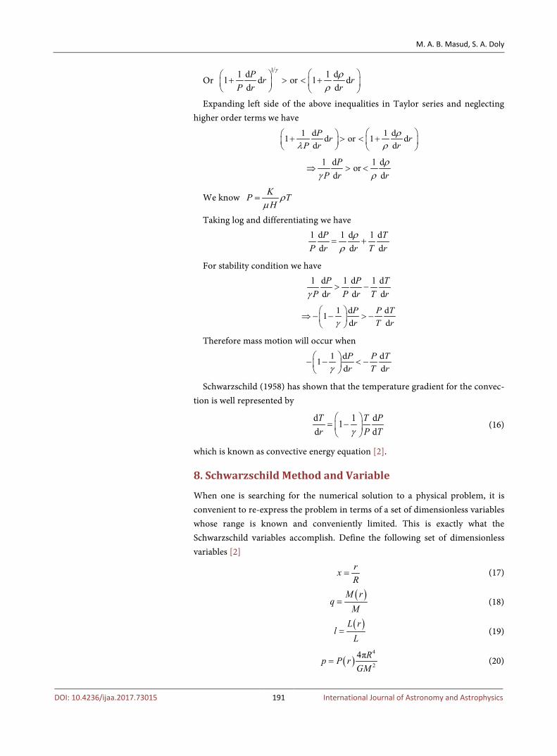
Schwarzschild (1958) has shown that the temperature gradient for the convec-tion is well represented by

d 1 d1d dT T Pr P Tγ

= −

(16)

which is known as convective energy equation [2].

8. Schwarzschild Method and Variable

When one is searching for the numerical solution to a physical problem, it is convenient to re-express the problem in terms of a set of dimensionless variables whose range is known and conveniently limited. This is exactly what the Schwarzschild variables accomplish. Define the following set of dimensionless variables [2]

rxR

= (17)

( )M rq

M= (18)

( )L rl

L= (19)

( )4

2

4πRp P rGM

= (20)




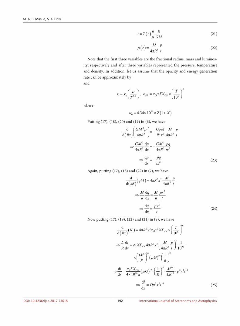
( ) R Rt T rGMµ

= (21)

( ) 34πM pr

tRρ = (22)

Note that the first three variables are the fractional radius, mass and luminos-ity, respectively and after three variables represented the pressure, temperature and density. In addition, let us assume that the opacity and energy generation rate can be approximately by and

0 3.5Tρκ κ =

,

16

0 610PP CNTXXε ε ρ = ×

where

( )250 4.34 10 1Z Xκ = × × +

Putting (17), (18), (20) and (19) in (6), we have

( )2

4 2 2 3

dd 4π 4π

GM p GqM M pRx tR R x R

= −

2 2

5 5 2

dd4π 4π

GM p GM pqxR R tx

⇒ = −

2

ddp pqx tx

⇒ = − (23)

Again, putting (17), (18) and (22) in (7), we have

( ) ( ) 2 23

d 4πd 4π

M pqM R xxR tR

=

2dd

M q M pxR x R t

⇒ =

2ddq pxx t

⇒ = (24)

Now putting (17), (19), (22) and (21) in (8), we have

( ) ( )16

2 2 20 6

d 4πd 10CN

TlL R x XXRx

ε ρ = ×

( )

22 2

0 3 96

16 1616

d 14πd 4π 10

1

CNL l M pXX R xR x tR

tM GR R

ε

µ

⇒ =

×

( )16 18

16 2 2 14096 19

d 1d 4 10 π

CNXXl MG p x tx R LR

εµ ⇒ = ⋅ ⋅ ⋅ ×

2 2 14dd

l Dp x tx

⇒ = (25)




where ( )16 18

16096 19

14 10 π

CNXX MD GR LR

εµ = × × × ×

Again putting (17), (19), (21), (22) and (23) in (15), we get

( )2

02 2 6.5

3dd 16π

lLGMtRx R R acR x T

κµ ρ = − ×

6.52 6.50

2 3

3dd 16π 4π

lLt M p R RGMR x t GMtacx R

κµµ

⇒ = − × × ×

7.5 0.5 203 5.5 2 8.5

3d 1d 256π

t LR p lx Gac M x t

κ ⇒ = −

2

2 8.5

dd

t p lCx x t

⇒ = −

where 7.5 0.5

03 5.5

3 1256π

LRCGac M

κ =

putting (17), (19) and (20) in (16) we have

d 2 dd 5 d

t t px p x= (26)

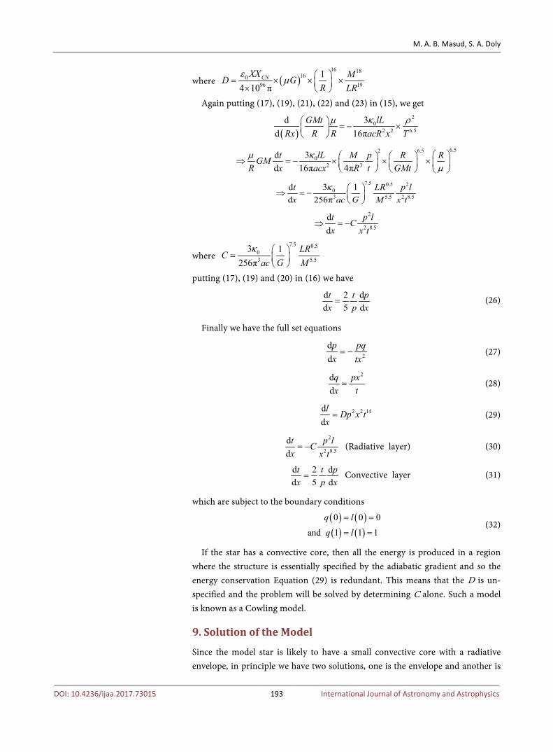
Finally we have the full set equations

2

ddp pqx tx= − (27)

2ddq pxx t= (28)

2 2 14dd

l Dp x tx= (29)

2

2 8.5

dd

t p lCx x t= − (Radiative layer) (30)

d 2 dd 5 d

t t px p x= Convective layer (31)

which are subject to the boundary conditions

( ) ( )( ) ( )0 0 0

and 1 1 1

q l

q l

= =

= = (32)

If the star has a convective core, then all the energy is produced in a region where the structure is essentially specified by the adiabatic gradient and so the energy conservation Equation (29) is redundant. This means that the D is un-specified and the problem will be solved by determining C alone. Such a model is known as a Cowling model.

9. Solution of the Model

Since the model star is likely to have a small convective core with a radiative envelope, in principle we have two solutions, one is the envelope and another is




the core. The two solutions must match at the interface. a) Polytropic Core Solution b) Packet Solution

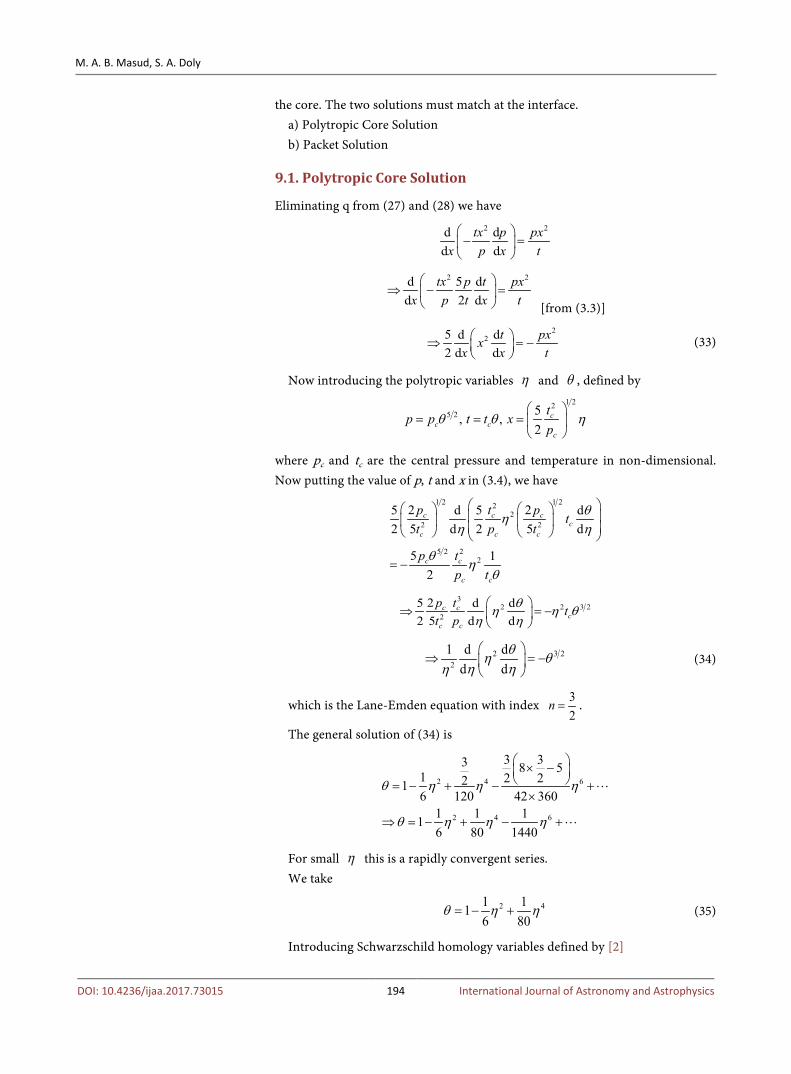
9.1. Polytropic Core Solution

Eliminating q from (27) and (28) we have 2 2d d

d dtx p px

x p x t − =

2 2d 5 dd 2 d

tx p t pxx p t x t

⇒ − = [from (3.3)]

225 d d

2 d dt pxx

x x t ⇒ = −

(33)

Now introducing the polytropic variables η and θ , defined by 1 22

5 2 5, ,2

cc c

c

tp p t t xp

θ θ η

= = =

where pc and tc are the central pressure and temperature in non-dimensional. Now putting the value of p, t and x in (3.4), we have

1 2 1 222

2 2

5 2 22

2 25 d 5 d2 d 2 d5 5

5 12

c c cc

cc c

c c

c c

p t p tpt t

p tp t

θηη η

θη

θ

= −

32 2 3 2

2

25 d d2 d d5

c cc

cc

p t tpt

θη η θη η

⇒ = −

2 3 22

1 d dd d

θη θη ηη

⇒ = −

(34)

which is the Lane-Emden equation with index 32

n = .

The general solution of (34) is

2 4 6

2 4 6

3 33 8 51 2 2216 120 42 360

1 1 116 80 1440

θ η η η

θ η η η

× − = − + − +

×

⇒ = − + − +

�

�

For small η this is a rapidly convergent series. We take

2 41 116 80

θ η η= − + (35)

Introducing Schwarzschild homology variables defined by [2]




( )( )

( )

2 2 2

22 2

1 25 2 2

1 22

2 23 2 3 2

2

d ln d d dd ln d d d

2 1d 5 d d5dd 2 d dd

2 5 1d5 2d5

22 5 1 1 33

d d5 2 10d d

c c

cc c

c

c

c c

cc

M r M rr xR M q x qUr M r r qM R x q x

x px p x p x pxp p t tt ttx p t tx t x xp x

p ttt ptp

p tpt

θη

θθη

ηθ η θ ηθ θη η

≡ = = =

= − ⋅ = − = − = −

= −

= − = − ≅ − +�

( )( )

2

2 4

4

1 22 5 2

5 2 1 22

5 2 2 2

5 2

d ln d dandd ln d d4π

4π2.5d d

d 2.5 d

d 5 1d 6 60

c c

c c c

P r P xR GM pVr P r R xGM Rp

Rt px p

p x p t p

η θθ η

η θ η ηηθ

≡ − = − = −

= − = −

= − ≅ + +

�

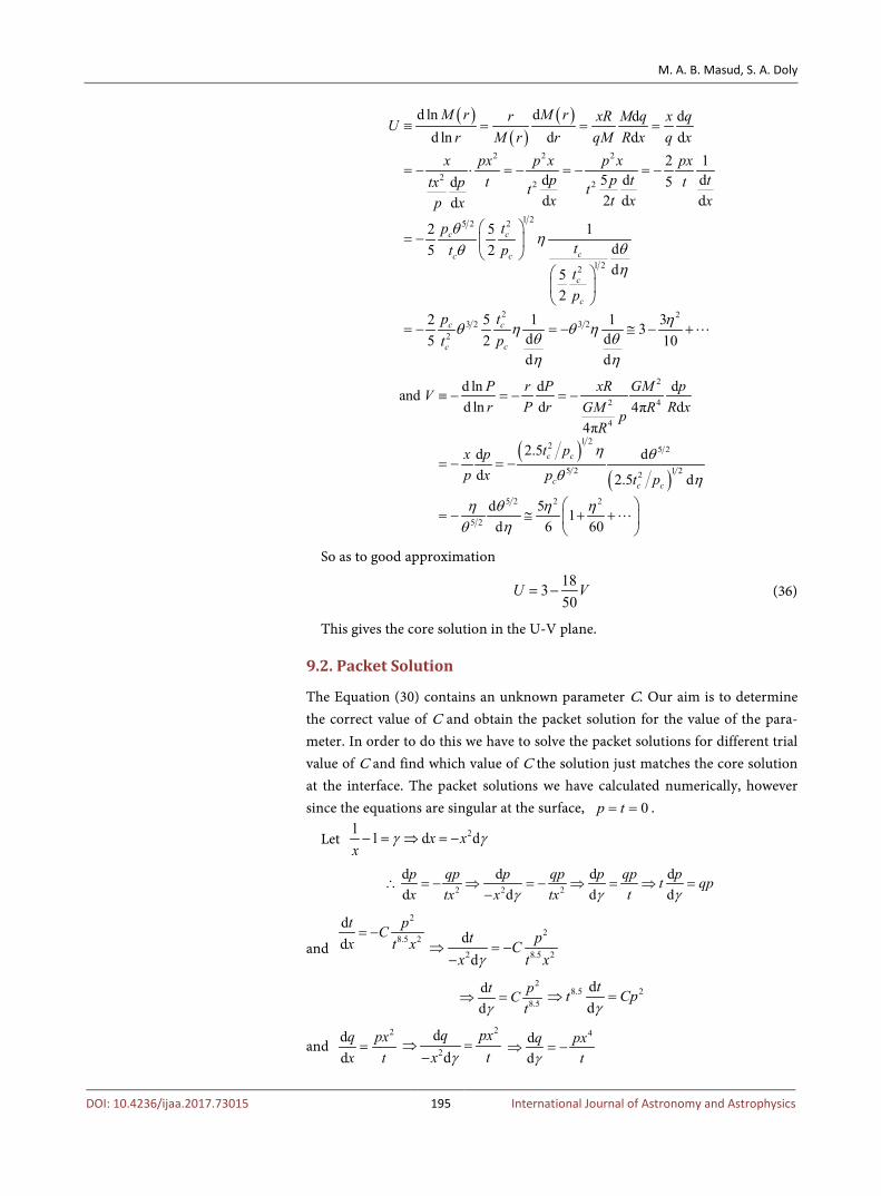
So as to good approximation

18350

U V= − (36)

This gives the core solution in the U-V plane.

9.2. Packet Solution

The Equation (30) contains an unknown parameter C. Our aim is to determine the correct value of C and obtain the packet solution for the value of the para-meter. In order to do this we have to solve the packet solutions for different trial value of C and find which value of C the solution just matches the core solution at the interface. The packet solutions we have calculated numerically, however since the equations are singular at the surface, 0p t= = .

Let 21 1 d dx xx

γ γ− = ⇒ = −

2 2 2

d d d dd d ddp qp p qp p qp pt qpx ttx x tx γ γγ

∴ = − ⇒ = − ⇒ = ⇒ =−

and

2

8.5 2

dd

t pCx t x= − 2

2 8.5 2

ddt pC

x t xγ⇒ = −

−

2

8.5

dd

t pCtγ

⇒ = 8.5 2dd

tt Cpγ

⇒ =

and 2d

dq pxx t=

2

2

ddq px

tx γ⇒ =

−

4dd

q pxtγ

⇒ = −




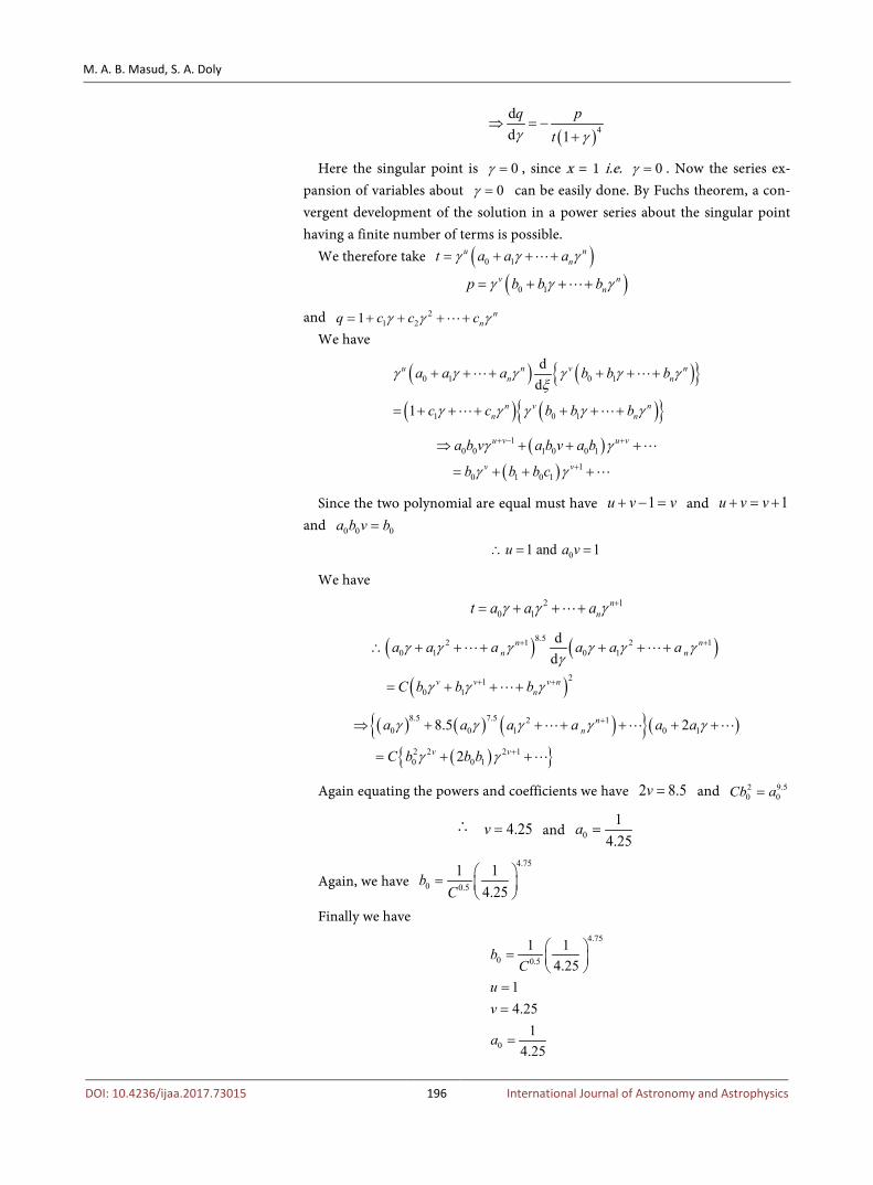
( )4

dd 1

q ptγ γ

⇒ = −+

Here the singular point is 0γ = , since x = 1 i.e. 0γ = . Now the series ex-pansion of variables about 0γ = can be easily done. By Fuchs theorem, a con-vergent development of the solution in a power series about the singular point having a finite number of terms is possible.

We therefore take ( )0 1u n

nt a a aγ γ γ= + + +�

( )0 1v n

np b b bγ γ γ= + + +�

and 21 21 n

nq c c cγ γ γ= + + + +� We have

( ) ( ){ }( ) ( ){ }

0 1 0 1

1 0 1

dd

1

u n v nn n

n v nn n

a a a b b b

c c b b b

γ γ γ γ γ γξ

γ γ γ γ γ

+ + + + + +

= + + + + + +

� �

� �

( )( )

10 0 1 0 0 1

10 1 0 1

u v u v

v v

a b v a b v a b

b b b c

γ γ

γ γ

+ − +

+

⇒ + + +

= + + +

�

� Since the two polynomial are equal must have 1u v v+ − = and 1u v v+ = +

and 0 0 0a b v b=

01 and 1u a v∴ = = We have

2 10 1

nnt a a aγ γ γ += + + +�

( ) ( )

( )

8.52 1 2 10 1 0 1

210 1

dd

n nn n

v v v nn

a a a a a a

C b b b

γ γ γ γ γ γγ

γ γ γ

+ +

+ +

∴ + + + + + +

= + + +

� �

�

( ) ( ) ( ){ }( )

( ){ }

8.5 7.5 2 10 0 1 0 1

2 2 2 10 0 1

8.5 2

2

nn

v v

a a a a a a

C b b b

γ γ γ γ γ

γ γ

+

+

⇒ + + + + + +

= + +

� � �

�

Again equating the powers and coefficients we have 2 8.5v = and 2 9.50 0Cb a=

∴ 4.25v = and 01

4.25a =

Again, we have 4.75

0 0.5

1 14.25

bC

=

Finally we have 4.75

0 0.5

0

1 14.25

14.25

14.25

bC

uv

a

=

==

=




Therefore, in the first approximation we have about 0γ = , i.e. 1x = 4.75

4.250 0.5

4.75 4.75

0.5

1 14.25

1 1 1 14.25

vp bC

xC

γ γ ≈ =

= −

and 01 1 1 1

4.25 4.25ut a

xγ γ ≈ = = −

and 1q ≈ Here C as a free parameter and consider of values of close to 10−6. We take a

point x = 0.99 very near to the surface. Appropriate for convection, by the fourth order Runge- Kutta method for a number of trial values of C. Some of these cal-culations, namely for 61.56eC −= , 75.6eC −= and 79.46eC −= .

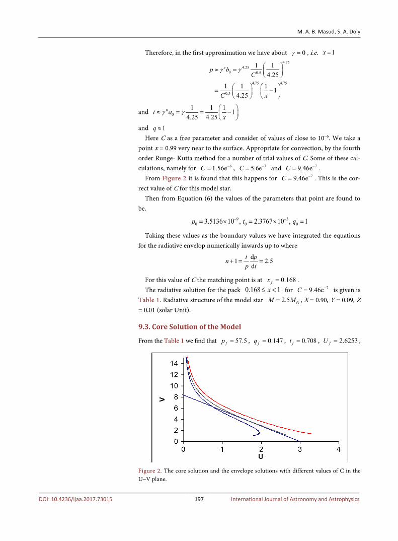
From Figure 2 it is found that this happens for 79.46eC −= . This is the cor-rect value of C for this model star.

Then from Equation (6) the values of the parameters that point are found to be.

9 30 0 03.5136 10 , 2.3767 10 , 1p t q− −= × = × =

Taking these values as the boundary values we have integrated the equations for the radiative envelop numerically inwards up to where

d1 2.5d

t pnp t

+ = =

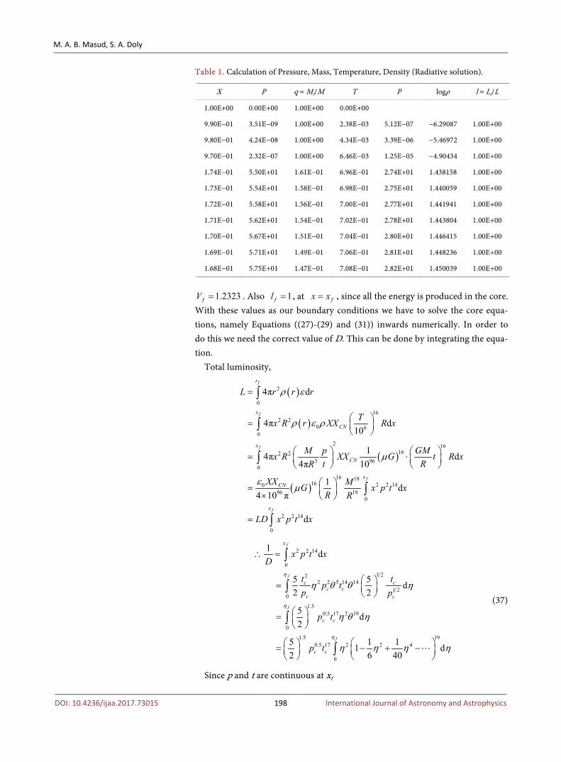
For this value of C the matching point is at 0.168fx = . The radiative solution for the pack 0.168 1x≤ < for 79.46eC −= is given is

Table 1. Radiative structure of the model star 2.5M M= � , X = 0.90, Y = 0.09, Z = 0.01 (solar Unit).

9.3. Core Solution of the Model

From the Table 1 we find that 57.5fp = , 0.147fq = , 0.708ft = , 2.6253fU = ,

Figure 2. The core solution and the envelope solutions with different values of C in the U−V plane.




Table 1. Calculation of Pressure, Mass, Temperature, Density (Radiative solution).

X P q = Mr/M T Ρ logρ l = Lr/L

1.00E+00 0.00E+00 1.00E+00 0.00E+00

9.90E−01 3.51E−09 1.00E+00 2.38E−03 5.12E−07 −6.29087 1.00E+00

9.80E−01 4.24E−08 1.00E+00 4.34E−03 3.39E−06 −5.46972 1.00E+00

9.70E−01 2.32E−07 1.00E+00 6.46E−03 1.25E−05 −4.90434 1.00E+00

1.74E−01 5.50E+01 1.61E−01 6.96E−01 2.74E+01 1.438158 1.00E+00

1.73E−01 5.54E+01 1.58E−01 6.98E−01 2.75E+01 1.440059 1.00E+00

1.72E−01 5.58E+01 1.56E−01 7.00E−01 2.77E+01 1.441941 1.00E+00

1.71E−01 5.62E+01 1.54E−01 7.02E−01 2.78E+01 1.443804 1.00E+00

1.70E−01 5.67E+01 1.51E−01 7.04E−01 2.80E+01 1.446415 1.00E+00

1.69E−01 5.71E+01 1.49E−01 7.06E−01 2.81E+01 1.448236 1.00E+00

1.68E−01 5.75E+01 1.47E−01 7.08E−01 2.82E+01 1.450039 1.00E+00

1.2323fV = . Also 1fl = , at fx x= , since all the energy is produced in the core.

With these values as our boundary conditions we have to solve the core equa-tions, namely Equations ((27)-(29) and (31)) inwards numerically. In order to do this we need the correct value of D. This can be done by integrating the equa-tion.

Total luminosity,

( )

( )

( )

( )

2

0

162 2

0 60

2 16162 2

3 960

16 1816 2 2 140

96 190

2 2 14

0

4π d

4π d10

14π d4π 10

1 d4 10 π

d

f

f

f

f

f

r

x

CN

x

CN

xCN

x

L r r r

Tx R r XX R x

M p GMx R XX G t R xt RR

XX MG x p t xR R

LD x p t x

ρ ε

ρ ε ρ

µ

εµ

=

=

= ⋅

= ×

=

∫

∫

∫

∫

∫

2 2 14

0

1 222 2 5 14 14

1 20

1.50.5 17 2 19

0

1.5 190.5 17 2 2 4

0

1 d

5 5 d2 2

5 d2

5 1 11 d2 6 40

f

f

f

f

x

c cc c

c c

c c

c c

x p t xD

t tp t

p p

p t

p t

η

η

η

η θ θ η

η θ η

η η η η

∴ =

=

=

= − + −

∫

∫

∫

∫ �

(37)

Since p and t are continuous at xf




5 2 andf c f c fp p t tθ θ= = Also we have,

2 22 533 and 1

10 6 60f f

f f fU Vη η

η

= − + = + +

� �

Now substituting the value of Uf and Vf we get from the above equations, 1.20167fη = and hence we get from the above equations, 0.78539.fθ =

Therefore 5 2f cp p θ=

( )5 2 5 2

57.506 105.197230.78539

fc

pp

θ⇒ = = =

And f c ft t θ=

0.70834 0.90190.78539

fc

f

tt

θ⇒ = = =

Now substituting the value of cp , ct and fη in the Equation (37) and

evaluating the integrating using Simpson’s one third rules, we have

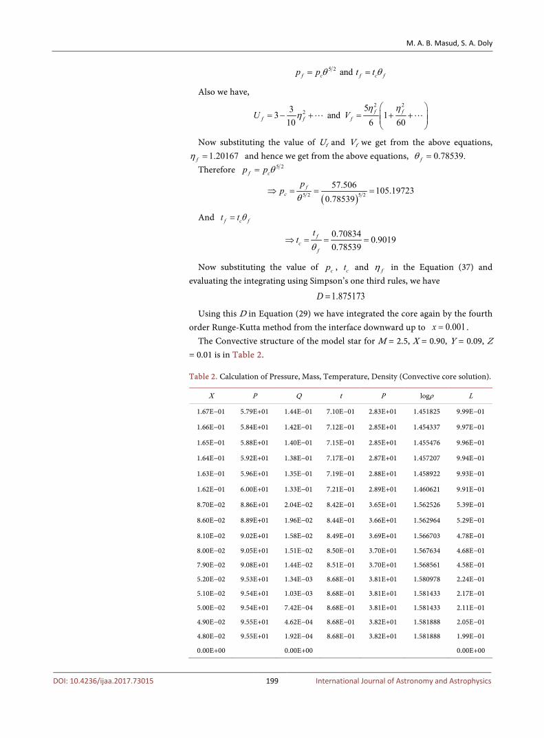
1.875173D = Using this D in Equation (29) we have integrated the core again by the fourth

order Runge-Kutta method from the interface downward up to 0.001x = . The Convective structure of the model star for M = 2.5, X = 0.90, Y = 0.09, Z

= 0.01 is in Table 2.

Table 2. Calculation of Pressure, Mass, Temperature, Density (Convective core solution).

X P Q t Ρ logρ L

1.67E−01 5.79E+01 1.44E−01 7.10E−01 2.83E+01 1.451825 9.99E−01

1.66E−01 5.84E+01 1.42E−01 7.12E−01 2.85E+01 1.454337 9.97E−01

1.65E−01 5.88E+01 1.40E−01 7.15E−01 2.85E+01 1.455476 9.96E−01

1.64E−01 5.92E+01 1.38E−01 7.17E−01 2.87E+01 1.457207 9.94E−01

1.63E−01 5.96E+01 1.35E−01 7.19E−01 2.88E+01 1.458922 9.93E−01

1.62E−01 6.00E+01 1.33E−01 7.21E−01 2.89E+01 1.460621 9.91E−01

8.70E−02 8.86E+01 2.04E−02 8.42E−01 3.65E+01 1.562526 5.39E−01

8.60E−02 8.89E+01 1.96E−02 8.44E−01 3.66E+01 1.562964 5.29E−01

8.10E−02 9.02E+01 1.58E−02 8.49E−01 3.69E+01 1.566703 4.78E−01

8.00E−02 9.05E+01 1.51E−02 8.50E−01 3.70E+01 1.567634 4.68E−01

7.90E−02 9.08E+01 1.44E−02 8.51E−01 3.70E+01 1.568561 4.58E−01

5.20E−02 9.53E+01 1.34E−03 8.68E−01 3.81E+01 1.580978 2.24E−01

5.10E−02 9.54E+01 1.03E−03 8.68E−01 3.81E+01 1.581433 2.17E−01

5.00E−02 9.54E+01 7.42E−04 8.68E−01 3.81E+01 1.581433 2.11E−01

4.90E−02 9.55E+01 4.62E−04 8.68E−01 3.82E+01 1.581888 2.05E−01

4.80E−02 9.55E+01 1.92E−04 8.68E−01 3.82E+01 1.581888 1.99E−01

0.00E+00 0.00E+00 0.00E+00




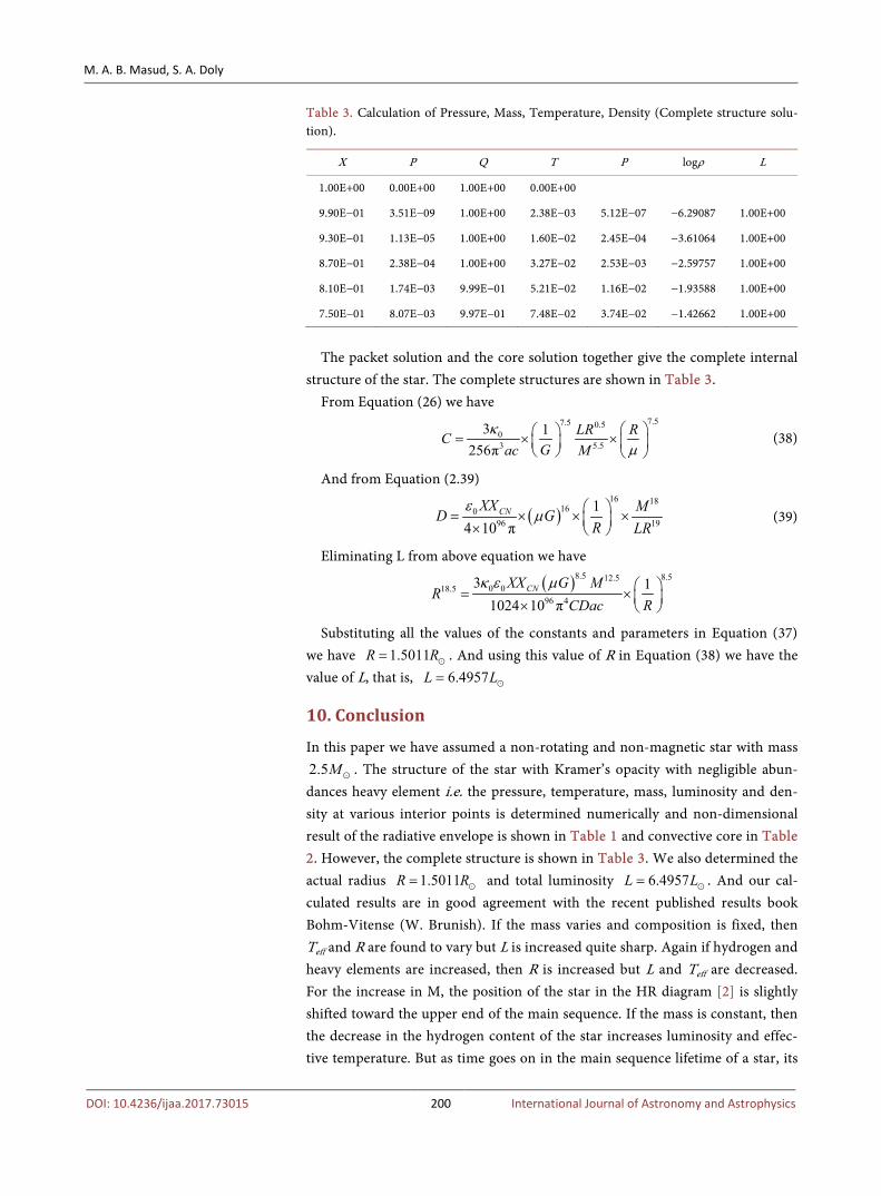
Table 3. Calculation of Pressure, Mass, Temperature, Density (Complete structure solu-tion).

X P Q T Ρ logρ L

1.00E+00 0.00E+00 1.00E+00 0.00E+00

9.90E−01 3.51E−09 1.00E+00 2.38E−03 5.12E−07 −6.29087 1.00E+00

9.30E−01 1.13E−05 1.00E+00 1.60E−02 2.45E−04 −3.61064 1.00E+00

8.70E−01 2.38E−04 1.00E+00 3.27E−02 2.53E−03 −2.59757 1.00E+00

8.10E−01 1.74E−03 9.99E−01 5.21E−02 1.16E−02 −1.93588 1.00E+00

7.50E−01 8.07E−03 9.97E−01 7.48E−02 3.74E−02 −1.42662 1.00E+00

The packet solution and the core solution together give the complete internal

structure of the star. The complete structures are shown in Table 3. From Equation (26) we have

7.57.5 0.503 5.5

3 1256π

LR RCGac M

κµ

= × ×

(38)

And from Equation (2.39)

( )16 18

16096 19

14 10 π

CNXX MD GR LR

εµ = × × × ×

(39)

Eliminating L from above equation we have

( )8.5 8.512.50 018.5

96 4

3 11024 10 π

CNXX G MR

RCDacκ ε µ = × ×

Substituting all the values of the constants and parameters in Equation (37) we have 1.5011R R= � . And using this value of R in Equation (38) we have the value of L, that is, 6.4957L L= �

10. Conclusion

In this paper we have assumed a non-rotating and non-magnetic star with mass 2.5M� . The structure of the star with Kramer’s opacity with negligible abun-dances heavy element i.e. the pressure, temperature, mass, luminosity and den-sity at various interior points is determined numerically and non-dimensional result of the radiative envelope is shown in Table 1 and convective core in Table 2. However, the complete structure is shown in Table 3. We also determined the actual radius 1.5011R R= � and total luminosity 6.4957L L= � . And our cal-culated results are in good agreement with the recent published results book Bohm-Vitense (W. Brunish). If the mass varies and composition is fixed, then Teff and R are found to vary but L is increased quite sharp. Again if hydrogen and heavy elements are increased, then R is increased but L and Teff are decreased. For the increase in M, the position of the star in the HR diagram [2] is slightly shifted toward the upper end of the main sequence. If the mass is constant, then the decrease in the hydrogen content of the star increases luminosity and effec-tive temperature. But as time goes on in the main sequence lifetime of a star, its




hydrogen content gradually diminishes giving rise to the helium content. That means, a main sequence of star ages, which positions in the HR diagram, slowly moves along the main sequence toward the hot end.

References [1] Böhm-Vitense, E. (1992) Introduction to Stellar Astrophysics. Volume 3, Stellar

Structure and Evolution, Cambridge University Press, Cambridge.

[2] Reeves, H. (1964) Stellar Energy Sources. In: Schwarzschild, M., Howard, R. and Harm, R., Eds., Stellar Structure, Vol. 3, 233.

[3] Chandrasekhar, S. (1989) Stellar Structure and Stellar Atmospheres. Volume 1, University of Chicago Press, Chicago.

[4] Bethe, H.A. (1939) Energy Production in Stars. Physical Review, 55, 425.

[5] Kippenhahn, R. and Weigert, A. (1990) Stellar Structure and Evolution. Vol. 16, Springer-Verlag Berlin, Heidelberg, New York, 468.

[6] Hansen, C.J., Kawaler, S.D. and Trimble, V. (2004) Stellar Interiors. 2nd Edition, Springer, New York. https://doi.org/10.1007/978-1-4419-9110-2

[7] Kippenhahn, R. and Weigert, A. (1990) Stellar Structure and Evolution.

Submit or recommend next manuscript to SCIRP and we will provide best service for you:

Accepting pre-submission inquiries through Email, Facebook, LinkedIn, Twitter, etc. A wide selection of journals (inclusive of 9 subjects, more than 200 journals) Providing 24-hour high-quality service User-friendly online submission system Fair and swift peer-review system Efficient typesetting and proofreading procedure Display of the result of downloads and visits, as well as the number of cited articles Maximum dissemination of your research work

Submit your manuscript at: http://papersubmission.scirp.org/ Or contact [email protected]


https://doi.org/10.1007/978-1-4419-9110-2

http://papersubmission.scirp.org/

mailto:[email protected]

Documents

A Study of Stellar Model with Kramer’s Opacity by Using ... · DOI: 10.4236/ijaa.2017.73015 Sep. 11, 2017 185 International Journal of Astronomy and Astrophysics A Study of Stellar