Embed Size (px)
Citation preview
Atmos. Chem. Phys., 7, 4977–5002, 2007www.atmos-chem-phys.net/7/4977/2007/© Author(s) 2007. This work is licensedunder a Creative Commons License.
AtmosphericChemistry
and Physics
A study of the effect of overshooting deep convection on the watercontent of the TTL and lower stratosphere from Cloud ResolvingModel simulations
D. P. Grosvenor1, T. W. Choularton1, H. Coe1, and G. Held2
1The University of Manchester, Manchester, UK2Instituto de Pesquisas Meteorologicas, Universidade Estadual Paulista, 17015-970 BAURU, S.P., Brasil
Received: 4 May 2007 – Published in Atmos. Chem. Phys. Discuss.: 30 May 2007Revised: 12 September 2007 – Accepted: 17 September 2007 – Published: 28 September 2007
Abstract. Simulations of overshooting, tropical deep con-vection using a Cloud Resolving Model with bulk micro-physics are presented in order to examine the effect on thewater content of the TTL (Tropical Tropopause Layer) andlower stratosphere. This case study is a subproject of theHIBISCUS (Impact of tropical convection on the upper tro-posphere and lower stratosphere at global scale) campaign,which took place in Bauru, Brazil (22◦ S, 49◦ W), from theend of January to early March 2004.
Comparisons between 2-D and 3-D simulations suggestthat the use of 3-D dynamics is vital in order to capturethe mixing between the overshoot and the stratospheric air,which caused evaporation of ice and resulted in an overallmoistening of the lower stratosphere. In contrast, a dehy-drating effect was predicted by the 2-D simulation due to theextra time, allowed by the lack of mixing, for the ice trans-ported to the region to precipitate out of the overshoot air.
Three different strengths of convection are simulated in3-D by applying successively lower heating rates (used toinitiate the convection) in the boundary layer. Moistening isproduced in all cases, indicating that convective vigour is nota factor in whether moistening or dehydration is producedby clouds that penetrate the tropopause, since the weakestcase only just did so. An estimate of the moistening effectof these clouds on an air parcel traversing a convective re-gion is made based on the domain mean simulated moisten-ing and the frequency of convective events observed by theIPMet (Instituto de Pesquisas Meteorologicas, UniversidadeEstadual Paulista) radar (S-band type at 2.8 Ghz) to have thesame 10 dBZ echo top height as those simulated. These sug-gest a fairly significant mean moistening of 0.26, 0.13 and0.05 ppmv in the strongest, medium and weakest cases, re-spectively, for heights between 16 and 17 km. Since thecold point and WMO (World Meteorological Organization)
Correspondence to:D. P. Grosvenor([email protected])
tropopause in this region lies at∼15.9 km, this is likely torepresent direct stratospheric moistening. Much more moist-ening is predicted for the 15–16 km height range with in-creases of 0.85–2.8 ppmv predicted. However, it would berequired that this air is lofted through the tropopause via theBrewer Dobson circulation in order for it to have a strato-spheric effect. Whether this is likely is uncertain and, in ad-dition, the dehydration of air as it passes through the coldtrap and the number of times that trajectories sample con-vective regions needs to be taken into account to gauge theoverall stratospheric effect. Nevertheless, the results suggesta potentially significant role for convection in determiningthe stratospheric water content.
Sensitivity tests exploring the impact of increased aerosolnumbers in the boundary layer suggest that a correspondingrise in cloud droplet numbers at cloud base would increasethe number concentrations of the ice crystals transported tothe TTL, which had the effect of reducing the fall speeds ofthe ice and causing a∼13% rise in the mean vapour increasein both the 15–16 and 16–17 km height ranges, respectively,when compared to the control case. Increases in the totalwater were much larger, being 34% and 132% higher forthe same height ranges, but it is unclear whether the extraice will be able to evaporate before precipitating from theregion. These results suggest a possible impact of naturaland anthropogenic aerosols on how convective clouds affectstratospheric moisture levels.
1 Introduction
The amount of water vapour in the stratosphere can signif-icantly affect the Earth’s climate since it is the most impor-tant greenhouse gas in the atmosphere. Additionally, it is oneof the main sources of ozone destroying OH hydroxyl radi-cals and is involved in the formation of Polar StratosphericClouds, which also help to destroy ozone.
Published by Copernicus Publications on behalf of the European Geosciences Union.
4978 D. P. Grosvenor et al.: Modeling the effects of deep convection on TTL water content
Understanding what affects the stratospheric water vapourcontent is therefore vitally important, even more so in lightof observations that suggest that it has been increasing by∼1% per year over the past 50 years (Oltmans and Hof-mann, 1995; Rosenlof et al., 2001). About half of this isattributed to changes in the processes affecting the entry ofwater vapour into the stratosphere from the troposphere, withthe rest due to increases in methane amounts. Determiningwhat affects the vapour content during troposphere to strato-sphere transport then becomes key to understanding this in-crease and hence how it might alter in a changing climate.
To date the tropical slow uplift and “freeze-drying” mech-anism of Brewer (1949) is still accepted as broadly control-ling the amount of water vapour entering the stratosphere.Here vapour is assumed to be reduced towards the relativelylow ice saturation mixing ratios at the cold temperaturesof the tropical tropopause by ice formation and subsequentvapour deposition, with the ice falling out of the rising air.
Trajectory studies based on ECMWF model wind andtemperature fields (Fueglistaler et al., 2004) suggested that70% of the air parcels traversing from the troposphere tothe stratosphere reached their minimum temperature overthe western Pacific, where the coldest tropopause tempera-tures are found, but found no evidence for the majority alsocrossing the tropopause in that region and hence little evi-dence for the “stratospheric fountain” region (as proposed byNewell and Gould-Stewart, 1981). This is feasible becausethe slow uplift rate of the Brewer Dobson circulation (meanglobal scale velocity of∼0.5 mm s−1) combined with rela-tively large horizontal winds of the order of 5 m s−1 allowsair parcels to travel horizontal distances of several thousandkilometres whilst ascending vertically by only a few hundredmetres (Holton and Gettelman, 2001).
Furthermore, the water vapour mixing ratios of trajectorieson entry into the stratosphere, as reported in Fueglistaler etal. (2004), Fueglistaler and Haynes (2005) and Fueglistaler etal. (2005), were found to be broadly consistent with satelliteobservations of the lower stratospheric vapour content. Thissuggests that processes that potentially affect stratosphericvapour content, but which are not included in the ECMWFmodel, such as the effects of deep convection or the mi-crophysical details of ice formation and sedimentation, maybe of secondary importance compared to the environmentaltemperature experienced by air during troposphere to strato-sphere transport.
A potential problem comes from the fact that the cor-relation between mean tropopause temperatures and strato-spheric vapour mixing ratios found in Fueglistaler andHaynes (2005) is at odds with the observed long-term in-crease in stratospheric water vapour in light of mean tropicaltropopause temperatures from radiosonde observations thathave been reported as decreasing by∼0.57 K decade−1 be-tween 1973–1998 (Zhou et al., 2001) or by∼0.5 K decade−1
between 1978–1997 (Seidel et al., 2001). Using trajectoriesbased in the 1960s, Fueglistaler and Haynes (2005) found
no differences when compared to trajectories based in timescloser to the present that could account for the long-termtrend in water vapour, indicating that factors other than dy-namical pathways and the environmental temperature maybe of importance after all, unless the observed increases instratospheric water vapour are incorrect.
The effects of deep convection on the stratospheric watervapour entry mixing ratio is one such pathway that may of-fer an explanation of the long-term trend in water vapour.Dehydration of air entering the stratosphere by overshoot-ing deep convective clouds has been previously suggested byseveral authors, e.g. Danielsen (1982), Holton et al. (1995)and Sherwood and Dessler (2001). If convection overshootsits level of neutral buoyancy it becomes colder than the envi-ronment, thus possibly allowing dehydration down to lowervapour mixing ratios than would occur during slow ascentin equilibrium with the environment temperature. However,such clouds are likely to carry large amounts of ice into theTTL region and therefore, if sufficient ice is not removed bysedimentation, then there is also the possibility of moisteningof the air bound for the stratosphere.
Deep convective effects on the TTL water content arelikely to be much more complex than freeze drying linked tolow temperatures alone. Various dynamical and microphys-ical processes occurring in the clouds are involved, whichcould be affected by environmental changes throughout thetroposphere. Changes to these processes over long timescales could result in dehydration and/or moistening changesdespite trends in tropopause temperatures. One example is anincrease in aerosol loadings, which may have occurred due tothe increasing urbanisation of previously unspoilt areas in thetropics (Gupta, 2002) or through increases in biomass burn-ing (Sherwood, 2002), for example.
Aerosol increases may lead to smaller ice crystals beingtransported in the overshooting clouds, causing less dehydra-tion or more moistening due to the smaller ice failing to fallfrom the detrained air. Indeed, Sherwood (2002) found cor-relations between the stratospheric moisture content and theeffective diameter of ice crystals in the upper troposphere asmeasured by satellite instruments. The variations observedwere approximately semi-annular and hence not correlatedwith the tropopause temperature seasonal cycle, but ratherseemed to coincide with periods of biomass burning. In-creases in the latter have been observed over the same periodas the stratospheric water vapour increase, suggesting an ex-planation for the lack of correlation with tropopause temper-atures.
In this work a Cloud Resolving Model (CRM) will be usedto examine how single overshooting deep convective cloudsmight affect the water content of the TTL. There have beenrelatively few such studies in the past. Kupper et al. (2004)used the same CRM as in this work and looked at the con-vective effect over a timescale of 100 days by running themodel to convective equilibrium. The results showed no con-vective dehydration and that the non-convective flux of water
Atmos. Chem. Phys., 7, 4977–5002, 2007 www.atmos-chem-phys.net/7/4977/2007/
D. P. Grosvenor et al.: Modeling the effects of deep convection on TTL water content 4979
through the cold point was several times greater than the con-vective flux, although the latter dominated at heights belowthere and hence possibly into the lower TTL. However, itis likely that the most vigorous of convection that occurs inreality over the continents of the tropics or in organised sys-tems was not represented. The modelling work presentedin this paper makes no attempt to simulate the frequency ofconvective events but does examine the effect of more vig-orous overshooting events. Wang (2003) used a CRM tolook at overshooting mid-latitude convection and found thatplumes of water vapour were produced in the stratospheredue to gravity wave breaking at the cloud top. Chaboureau etal. (2007) simulated an overshooting, deep convective eventusing a mesoscale model initialised using real meteorologi-cal conditions and based in the same area as the simulationspresented here, which suggested that such events might causea significant flux of water vapour into the stratosphere. Thecurrent work differs in that single idealised cells are simu-lated, which allows sensitivities to convective vigour and mi-crophysics to be investigated. In addition, the model usedhere allows for ice supersaturation, in contrast to the micro-physics scheme employed in Chaboureau et al. (2007).
Assessing the effect of deep convection on the stratosphereis more pertinent given recent data that suggests that con-vective penetration into the TTL occurs significantly morefrequently than previously thought (Dessler et al., 2006) andthat the amount of ice injected may be hydrologically impor-tant (Wu et al., 2005). CRMs probably represent the mostuseful modelling tool available for examination of the com-plex dynamical and microphysical details of how deep con-vection affects the water content of the TTL and the sensi-tivities involved. Before they can be employed with con-fidence, though, their suitability needs to be investigatedthrough comparisons to observations and exploration of thesensitivities to the set up of the models.
2 Model set up and the case study day
2.1 The LEM Cloud Resolving Model
The CRM being used in these studies is the UK Met Of-fice LEM (Large Eddy Model) v2.3, as described in Shuttsand Gray (1994), albeit with some modifications. It explic-itly solves for large-scale motions using a quasi-Boussinesqnon-hydrostatic equation set and parameterizes small-scalesub-grid turbulent motions based on the Smagorinsky-Lillyapproach. Details of this parameterization can be found inBrown et al. (1994). Surface boundary conditions are de-rived from the Monin-Obukhov similarity theory using theBusinger-Dyer functions. The upper boundary condition isof the form of a rigid lid, but with a damping layer in theupper domain to prevent reflection of gravity waves.
The LEM uses a bulk microphysics scheme, which pa-rameterises conversions between water vapour, liquid water
1050 mb1000 mb
900 mb
800 mb
700 mb
600 mb
500 mb
400 mb
350 mb
300 mb
250 mb
200 mb
150 mb
100 mb
75 mb
T = -13
0
T = -12
0
T = -11
0
T = -10
0
T = -90
T = -80
T = -70
T = -60
T = -50
T = -40
T = -30
T = -20
T = -10
T = 0
T = 10
T = 20
T = 30
T = 40
θ = -20
θ = -10
θ = 0
θ = 10
θ = 20
θ = 30
θ = 40
θ = 50
θ = 60
θ = 70
θ = 80
θ = 90
θ = 100
θ = 110
48.0036.0028.0020.0016.0012.009.006.004.002.501.500.800.400.200.10
0.05
0.03
0.02
0.01
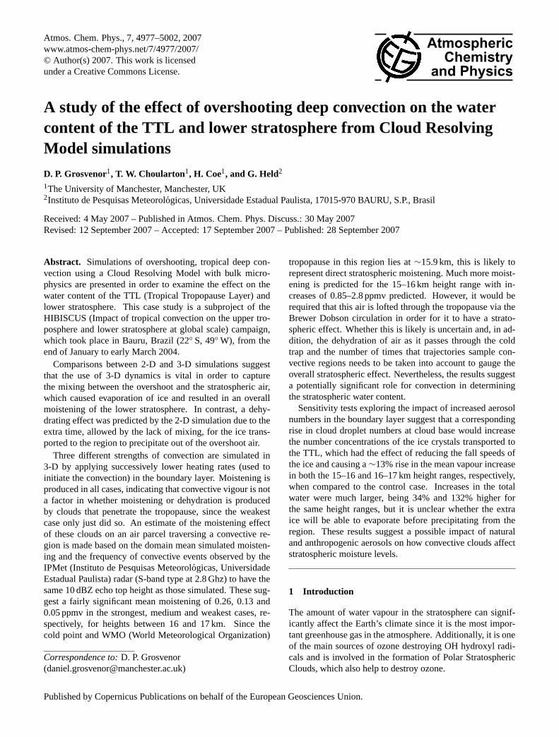
Fig. 1. Sounding from Bauru, 24 February 2004 at 20:15 UTC.
droplets, rain, ice (small ice crystals), snow (low density iceaggregates) and graupel (heavily rimed ice particles), as wellas their fall speeds. In order to do this, it assumes that thesize spectrum of each hydrometeor is a gamma-type func-tion with coefficients adjustable for each type. The model issingle moment for vapour, liquid and rain; i.e., it only hasvariables for their mass mixing ratios. It is double momentfor ice, snow and graupel, in that it can predict both theirmixing ratios and number concentrations. The ice scheme isbased on Lin et al. (1983), Rutledge and Hobbs (1984), Fer-rier (1994) and Ferrier et al. (1995), with refinements fromFlatau (1989), Swann (1996) and Swann (1998). The modelallows supersaturation of the vapour field with respect to icewith ice being heterogeneously nucleated as a function ofthis, as based on the Meyers et al. (1992) scheme. Vapourdeposition onto ice is based on the supersaturation, the massand number of the ice field and the assumed shape of the sizedistributions.
2.2 Meteorology and model initialisation
The simulations shown here were based on a case studyday of the 2004 HIBISCUS project, which took place inBauru, Brazil, located at 22.3◦ S, 49.03◦ W. The day cho-sen was 24 February, when a sounding (Fig.1) was madeat 20:15 UTC, which is 17:15 LT (local time). It shows apronounced dry layer centred at∼8.5 km with the cold pointand WMO tropopause occurring at∼15.9 km (112 mb – seethe end of this section for a discussion on the TTL location).The CAPE (Convective Available Potential Energy) of thesounding was a moderate 1095 J kg−1 and the presence of aninversion above the boundary layer resulted in CIN (Convec-tive Inhibition) of∼111 J kg−1.
Other radiosonde ascents performed on this day fromCampo Grande (610 km west-north-west of Bauru, at 00:00
www.atmos-chem-phys.net/7/4977/2007/ Atmos. Chem. Phys., 7, 4977–5002, 2007
4980 D. P. Grosvenor et al.: Modeling the effects of deep convection on TTL water content
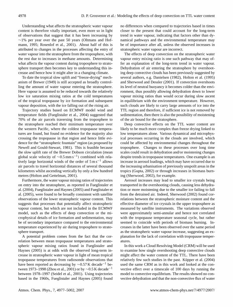
Fig. 2. Echo tops (reflectivity threshold 10 dBZ) observed by theS-band radar in Bauru at 19:38 UTC (=local time+3).
and 12:00 UTC as well as vertical profiles derived at 3-hourlyintervals from the Meso-Eta operational mesoscale model(Black, 1994) as run by CPTEC (Centre for Weather Fore-cast and Climatic Studies) for the South American conti-nent, showed CAPE values of between 1144 and 2389 J kg−1
throughout the day, signalling the potential for the devel-opment of severe storms. Cloud tops observed by IPMet’sradars (S-band type at 2.8 Ghz) were mostly<14 km, but afew cells penetrated through the tropopause (tops>18 kmat times) during the late afternoon (Fig.2). Cloud top es-timations from the radar are based on the 10 dBZ echo topfor which the errors should be within 1 km for 20 km highclouds at the edge of the radar range and considerably lessfor clouds that are lower or closer to the radar. Further de-scription of the storms that occurred on this day can be foundin Pommereau et al. (2007).
At the time of the radiosonde launch (20:15 UTC), theconvective area was≥100 km north-west to north-east ofthe radar, with echo tops mostly<10 km, but isolated cellsreached up to 15 km. The rain area south of Bauru wasalready in the dissipation stage. The convection continuedthroughout the night. Since the closest radiosonde available,viz. Bauru at 20:15 UTC, was released after the initiation ofconvective events, it is likely that there may be some discrep-ancies between these measurements and the environment thatthe storms actually formed in, especially in the lower layers,which are subject to heating and moistening, as well as low-level convergence processes.
The latter is known to be occurring in the region as a re-sult of the semi-stationary South Atlantic Convergence Zone(SACZ). This can be identified from satellite images as acloud band with orientation NW/SE, which commonly ex-tends from the southern region of Amazonia into the centralregion of the South Atlantic (Kousky, 1988), with a typi-cal persistence of≥4 days. It forms along the upper-level
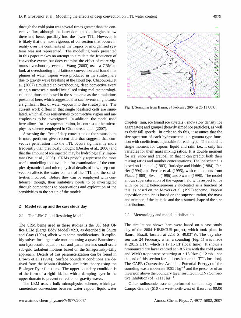
Fig. 3. TITAN-generated image (MDV format) of the storm com-plex on 24 February 2004 at 22:30 UTC. The ellipses demarcatecentroids of 20 dBZ reflectivity threshold with a minimum volumeof 16 km3.
subtropical jet and to the east of a semi-stationary troughover south-eastern South America, approximately along theBrazilian and Uruguayan coasts at 500 hPa. It is charac-terized by low-level humidity convergence zones, a stronggradient of the equivalent potential temperature in the mid-dle troposphere and an anticyclonic circulation at high levels(200 hPa). Being located at the edge of humid tropical airmasses, in regions of strong humidity gradients at low levels,it results in the generation of strong and extensive convectiveinstability. The occurrences of SACZ play an important rolein the transfer of latent heat, momentum and humidity fromthe tropics to the mid-latitudes and are responsible for themost humid periods and heavy summer rainfalls in the Stateof Sao Paulo.
Detailed analysis of radar-derived parameters, using IP-Met’s newly implemented software package TITAN (Thun-derstorm Identification, Tracking, Analysis and Nowcasting;Dixon and Wiener, 1993) with a 20 dBZ reflectivity thresholdand a volume of≥16 km3 for the identification of the cen-troid, confirmed the existence of a large multicellular stormcomplex, lasting for 14.6 h, with a maximum precipitationarea of 14 049 km2. Figure 3 depicts this complex in TI-TAN MDV format (Meteorological Data Volume; Dixon andWiener, 1993), shortly before reaching Bauru. The large el-lipsis demarcates the envelope of the 20 dBZ centroid, whichwas tracked to calculate the storm parameters. The Verti-cally Integrated Liquid water content (VIL), another indica-tor of severity, exceeded 7 kg m−2 (currently used at IPMet totrigger alerts; (Gomes and Held, 2004) on 11 occasions be-tween 18:57 and 24:07 UTC, with a maximum of 8.3 kg m−2
at 23:37 UTC.As the Bauru sounding showed some CIN and represented
the lower end of the range of CAPE suggested by sound-ings and mesoscale models, and since the aim here was to
Atmos. Chem. Phys., 7, 4977–5002, 2007 www.atmos-chem-phys.net/7/4977/2007/
D. P. Grosvenor et al.: Modeling the effects of deep convection on TTL water content 4981
simulate some extreme cases of convection, it was decidedto initiate convection by producing a warm and moist bub-ble in order to artificially increase the CAPE of the environ-ment and to help represent the influx of moist, tropical air ascaused by the SACZ. Warm bubbles have been used to ini-tiate deep convection in several CRM studies in the past. InWang (2003) a 20 km×4 km warm bubble of maximum per-turbation 3.5 K was imposed, which was made moister thanits surroundings since the relative humidity was kept con-stant as its temperature increased. In this study the bubblewas applied gradually using a heating and moistening rate inthe lower 2.5 km of the model domain over a width of 14 km,with the rate decreasing according to a cos2 relationship withradial distance from the centre. They were applied for twentyminutes, beginning 5 min after the simulation start and thesimulations were performed up to a time of 3 h 35 min. Runswith different heating rates, but with the same rate of mois-ture input, were performed in order to simulate convectionwith a variety of different strengths. These runs are labelled“3D-med” and “3D-weak” to indicate cells of medium andweaker intensity, with the original case labelled as “3-D”.
One 2-D case was simulated (labelled “2-D”) in whichthe model domain was 2000 km wide with a 2 km hori-zontal resolution. Such a large domain was required be-cause of interactions of gravity waves emanating from bothsides of the cloud due to the periodic boundary conditionsof the model, which interfered with the air from the over-shoot. This is much less of an issue in 3-D since the grav-ity waves produced are somewhat smaller in velocity mag-nitude than in 2-D. Therefore, in this case the domain is300×300 km in the “3-D” case and, for computational rea-sons, only 150×150 km in the “3D-med” and “3D-weak”sensitivity tests, with the same resolution. The vertical gridin all cases is 30.4 km deep with the damping layer appliedover the upper 7.6 km of the domain. The vertical resolutionwas 75 m in the boundary layer and 125 m throughout therest of the domain. Such high vertical resolution is likely tobe necessary to properly resolve processes occurring in theTTL, such as the effect of gravity waves on the temperaturestructure (e.g. Kuang and Bretherton, 2004), and thereforelikely on mixing processes too.
It has been demonstrated in previous CRM studies (e.g.Redelsperger et al., 2000), that the use of 2 km horizontal res-olution is fine enough to simulate deep convection reasonablywell. But, resolution can have a significant effect on convec-tive mixing processes (e.g. Petch et al., 2002) and thereforemay affect the turbulent mixing of overshoot air with the sur-roundings as well as the entrainment of environmental airinto the rising air parcel in the boundary layer as observed inCarpenter et al. (1998). The latter would be likely to lead toclouds that are too vigorous due to a lack of dilution by envi-ronmental air from higher levels. These processes would re-quire a resolution finer than 2 km to simulate explicitly (e.g.Lane et al., 2003, and Carpenter et al., 1998, use a horizontalgrid spacing of 50 m), although a sub-grid mixing parame-
terisation is included in the model, which may represent thisreasonably well. Also, the large ratio of horizontal to verticalgrid size may have an unknown effect on the vertical mix-ing and might therefore affect the mixing of overshoot air inthe TTL. In addition, Lane and Knievel (2005) suggest thatmodel resolution affects the spectra of gravity waves formedby CRM models, which can affect whether waves break ornot and hence whether mixing due to this process occurs.Further simulations to explore any potential sensitivities toresolution would be desirable, but were too computationallyexpensive for the current study.
Information on the various runs is displayed in Table 1.The “3D high CCN” case refers to a microphysical sensitiv-ity test case that uses the same heating rates for cloud ini-tiation as the “3-D” case and is described in Sect. 3.4. Asthe heating rate is decreased, the maximum vertical veloc-ity, which is 50 m s−1 in the most vigorous case, reduces toonly 39.3 and 28.4 m s−1, respectively, as the clouds becameless intense. 50 m s−1 represents a very high updraught, butone that is within the range of those inferred from obser-vations of tropical deep convection in other tropical regions(e.g. Simpson et al., 1993). The 10 dBZ echotop also reducesin height with cloud intensity from a maximum of 18.2 km toa minimum of 16.4 km in the “3D-weak” case. Interestingly,the 40 dBZ echotop is higher in the “3D-med” case than inthe more intense cloud. However, examination of the time-series of maximum echotop heights (not shown) reveals thatheights above 14 km were attained only very briefly in theweaker case (one data point in the timeseries where pointswere calculated every 5 min), whereas 14 km was reached bythe 40 dBZ contour for considerably longer in the “3-D” sim-ulation (for three data points in the timeseries).
As a result of the heating, a maximum temperature per-turbation of 7.2 K was produced in the “3-D” case, withsmaller perturbations in the cases with the lower heatingrates. Whilst this temperature increase is large, it is in linewith previous studies of very deep convection where simi-lar initiation methods were used. For example, maximumtemperature perturbations of up to 8 K were produced in thestudy of Robinson and Sherwood (2006) where heating rateswere applied for over an hour over a 100 km long area. Afurther indication of the vigour of the convection producedby the heating and moistening is given by the mean CAPEvalues for the different runs. These were calculated using themean profiles over the heating area and are shown after theheating had been applied for 5 min. Unfortunately, this datawas only available every 5 min and hence the peak CAPE val-ues may have been missed. The values show that the CAPEincreased from the original value of 1095 J kg−1 up to 2449–2687 J kg−1 in the 3-D cases and up to 3064 J kg−1 in the2-D case. The increase was larger in 2-D since the numberof points that are used in the average over the heating areais smaller. Whilst these increases are high, the CAPE val-ues are still quite moderate compared to other studies (e.g.Chaboureau, 2007) and for the 3-D cases are close to the
www.atmos-chem-phys.net/7/4977/2007/ Atmos. Chem. Phys., 7, 4977–5002, 2007
4982 D. P. Grosvenor et al.: Modeling the effects of deep convection on TTL water content
Table 1. Information on the different simulations. Columns are the maximum updraught; maximum radar reflectivity; the maximum heightof the 10, 35 and 40 dBZ echo tops; the maximum temperature and vapour perturbations in the lower 2.5 km of the domain; and the meanCAPE over the heating area after 5 min of heating.
Run Maxupdraught(m/s)
Max dBZ Max height of echotop (km): Max tempperturbation(K)
Max vapourmixing ratioperturbation(g kg−1)
Mean CAPEover heatingarea(J kg−1)
10 dBZ 35 dBZ 40 dBZ
3-D 50 54.7 18.2 17.5 15.1 7.2 2.2 26872-D 21.2 53.5 17 13.2 9.7 8.9 2.5 30643-D-med 39.3 56 17.4 16.5 15.6 4.1 3.2 24803-D-weak 28.4 55.2 16.4 15.3 11.7 3.3 4.2 24493-D high CCN 46.3 54.5 18.2 15.9 13.4 7.2 2.2 2687
0 5 10 15 20
12
14
16
18
20
Mixing Ratio (ppmv)
Hei
ght (
km)
24th Feb vapour and ice saturation mixing ratios
Original Sounding 20:15-22:08 UTCIce SaturationLEM water vapour
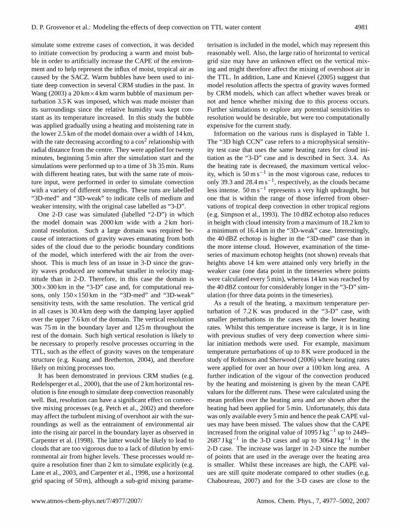
Fig. 4. Water vapour and ice saturation mixing ratio measurementsfrom the 24 February sounding and the idealised vapour profile in-put into the LEM Cloud Resolving Model.
upper range of those predicted by the Meso-Eta mesoscalemodel.
The main purpose of these simulations is to study the ef-fect of deep convection on the TTL water content. There-fore, in order to avoid the issue of determining whether re-ductions in total water were due to the ice deposition de-hydration effect, or simply due to reversible advection fromdrier heights, the simulations were initialised with a constantvapour mixing ratio of 5 ppmv around the TTL region, be-tween the heights of 15.77 and 18.93 km, as shown in Fig.4.This means that any reductions in the total water in this re-gion must have been due to the ice deposition dehydrationeffect and not reversible transport of the initial vapour field.The value of 5 ppmv corresponds to the approximate vapourmixing ratio in the sounding at the lower and upper boundaryof this region and is in line with other measurements of the
TTL water vapour concentrations made at 22:00 UTC at thesame location using the micro-SDLA instrument on boardanother balloon (Durry et al., 2006). This employs the diodelaser absorption spectroscopy technique and hence is likelyto be more accurate than standard radiosonde measurements,which used the Vaisala RS 80 package.
There are several different ways to define the TTL region,which is generally thought of as a transition zone containingair with both tropospheric and stratospheric properties. Themain concern here is how convection affects the water vapourcontent of air that will enter the stratosphere at some point inthe future and hence a useful definition for the TTL base isthat of the net zero radiative level (Zrad) as in Sherwood andDessler (2000). Based on several different radiation models,Gettelman et al. (2004) foundZrad to be located at a meanheight of 15 km in the tropics with differences due to timeand space variations leading to a±500 m change, and inter-model variations giving changes of±400 m. Whether thisapplies to the region of concern here, though, is unknown.
Since the main temperature inversion of the environmentis located at∼15.9 km (Fig.4) and significant changes in thevertical gradient of the water vapour mixing ratio are appar-ent here, this height is likely to generally serve as an efficientmixing barrier to weaker vertical motions and hence if con-vection affects air above this height then it will be very likelyto have a stratospheric effect. Therefore, this will be termedthe tropopause in future discussions here. According to theradar echo top heights, convection was observed to penetratethe tropopause and so the top of the TTL might be consideredto be somewhat higher than 15.9 km, following the conven-tion of Sherwood and Dessler (2000).
2.3 Radar observations
Radar statistics from the TroCCiBras/HIBISCUS field cam-paign (Held et al., 2006) show that, as in the “3-D” and “3D-med” cases, the 40 dBZ contour does reach 15 km and over in
Atmos. Chem. Phys., 7, 4977–5002, 2007 www.atmos-chem-phys.net/7/4977/2007/
D. P. Grosvenor et al.: Modeling the effects of deep convection on TTL water content 4983
Table 2. Frequencies of echo tops in the height ranges indicated for cell tracks within the 240 km radius range of the IPMet radar in Bauruduring the period from 21 January to 11 March 2004. Mean and max labels refer to the frequencies of the mean and maximum echo top ofeach track during the lifetime of the cell and 10, 35 and 40 dBZ refer to the tops of radar reflectivity contours of these values. Only cells witha volume larger than 50 km3, based on the 10, 35 and 40 dBZ contours, are included in the statistics.
Echo Top Echo Tops Echo Tops Echo Tops(km a.m.s.l.) 10 dBZ (%) 35 dBZ (%) 40 dBZ (%)
Mean Max Mean Max Mean Max
4 0.2 0.18 0.36 0.365 1.66 0.65 2.42 1.136 20.63 6.32 11.19 4.03 3.45 0.137 28.56 31.48 28.82 22.26 32.10 18.038 21.01 11.87 30.84 15.54 35.68 18.039 13.54 10.72 17.79 15.06 19.95 18.6710 8.07 16.46 6.24 23.63 6.14 25.7011 4.25 6.96 1.93 7.37 2.43 7.4212 1.45 5.63 0.28 4.43 0.26 5.8813 0.3 4.15 0.08 4.47 5.5014 0.19 1.29 0.04 0.81 0.5115 0.04 1.13 0.52 0.1316 0.03 1.94 0.4017 0.04 0.4818 0.01 0.2319 0.01 0.22≥20 0.01 0.29
Total no. of Tracks 10 198 2484 782
the Bauru area, albeit fairly infrequently. Table 2 shows thepercentages of the mean and maximum radar echo tops forthe 10, 35 and 40 dBZ reflectivity contours in certain heightranges, for cells where these contours contained storm vol-umes of≥50 km3. They were derived using the TITAN Soft-ware and are based on radar “tracks”, which is the term givento describe the following of a convective cell for its lifetime(including cell splits and mergers) by the software. A total of10 198, 2484 and 782 cells were identified, using the 10, 35and 40 dBZ threshold, respectively.
The data shows that the 40 dBZ echo top of one cell(0.13% of the 782 tracks) reached an absolute maximumheight of 15–16 km, with 0.64% (5 cells) exceeding 14 kmduring the 51 day observation period. In addition, the 35 dBZcontour in the “3-D” case reached higher than any of the ob-served events during the campaign (Table 1) and its maxi-mum height in the “3D-med” case (16.5 km) was consistentwith only 10 observed events over the campaign. Therefore,based on these higher reflectivities, events as severe as thosesimulated in the “3-D” and “3D-med” case may representthe upper limit of the convective effect of cells in this areaon the TTL region during the experimental period. However,the season in which the campaign took place was less activethan previously observed seasons as based on lightning (Nac-carato et al., 2004) and other observations (Pommereau et al.,
2007). Thus, clouds such as those modelled may have beenmore common in other years.
On the other hand, the maximum height reached by the10 dBZ contour in the “3-D” case (18.2 km) is consistentwith 75 of the observed cells over the campaign. This sug-gests that the model may be predicting too many particlesof high mass in the upper troposphere, but that the overallheights reached by the clouds are consistent with reality. Inaddition, factors such as the beam width divergence (beamwidth of radar = 2◦) and the possibility of radar scans miss-ing the peak development of clouds due to the time taken tocomplete a sweep (∼7.5 min), may result in the statistics notrepresenting the higher altitude, high reflectivity contours asconsistently as the output from the model.
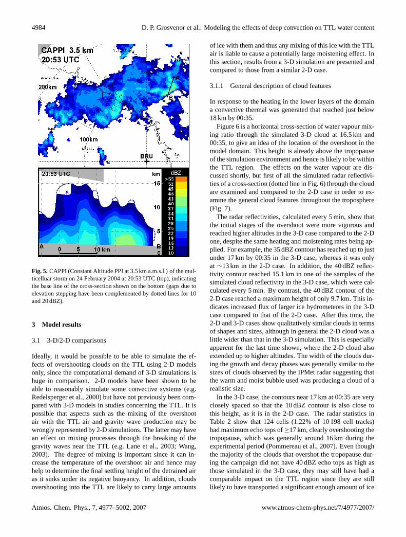
Figure5 shows a vertical cross-section through the stormcomplex at a time when it was quite mature and, in places,was almost 100 km wide at the altitude of 3.5 km. It shows a10 dBZ echo top that reaches up to∼15 km. The cell shownis fairly typical of those that occurred on 24 February withinthe radar range. There is little tilt of the updraught core, in-dicating fairly weak shear up to the heights involved. Thisslice is compared to the simulated radar reflectivity for thevarious runs in the following sections.
www.atmos-chem-phys.net/7/4977/2007/ Atmos. Chem. Phys., 7, 4977–5002, 2007
4984 D. P. Grosvenor et al.: Modeling the effects of deep convection on TTL water content
Fig. 5. CAPPI (Constant Altitude PPI at 3.5 km a.m.s.l.) of the mul-ticelluar storm on 24 February 2004 at 20:53 UTC (top), indicatingthe base line of the cross-section shown on the bottom (gaps due toelevation stepping have been complemented by dotted lines for 10and 20 dBZ).
3 Model results
3.1 3-D/2-D comparisons
Ideally, it would be possible to be able to simulate the ef-fects of overshooting clouds on the TTL using 2-D modelsonly, since the computational demand of 3-D simulations ishuge in comparison. 2-D models have been shown to beable to reasonably simulate some convective systems (e.g.Redelsperger et al., 2000) but have not previously been com-pared with 3-D models in studies concerning the TTL. It ispossible that aspects such as the mixing of the overshootair with the TTL air and gravity wave production may bewrongly represented by 2-D simulations. The latter may havean effect on mixing processes through the breaking of thegravity waves near the TTL (e.g. Lane et al., 2003; Wang,2003). The degree of mixing is important since it can in-crease the temperature of the overshoot air and hence mayhelp to determine the final settling height of the detrained airas it sinks under its negative buoyancy. In addition, cloudsovershooting into the TTL are likely to carry large amounts
of ice with them and thus any mixing of this ice with the TTLair is liable to cause a potentially large moistening effect. Inthis section, results from a 3-D simulation are presented andcompared to those from a similar 2-D case.
3.1.1 General description of cloud features
In response to the heating in the lower layers of the domaina convective thermal was generated that reached just below18 km by 00:35.
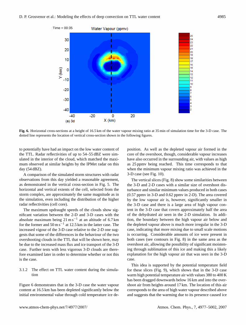
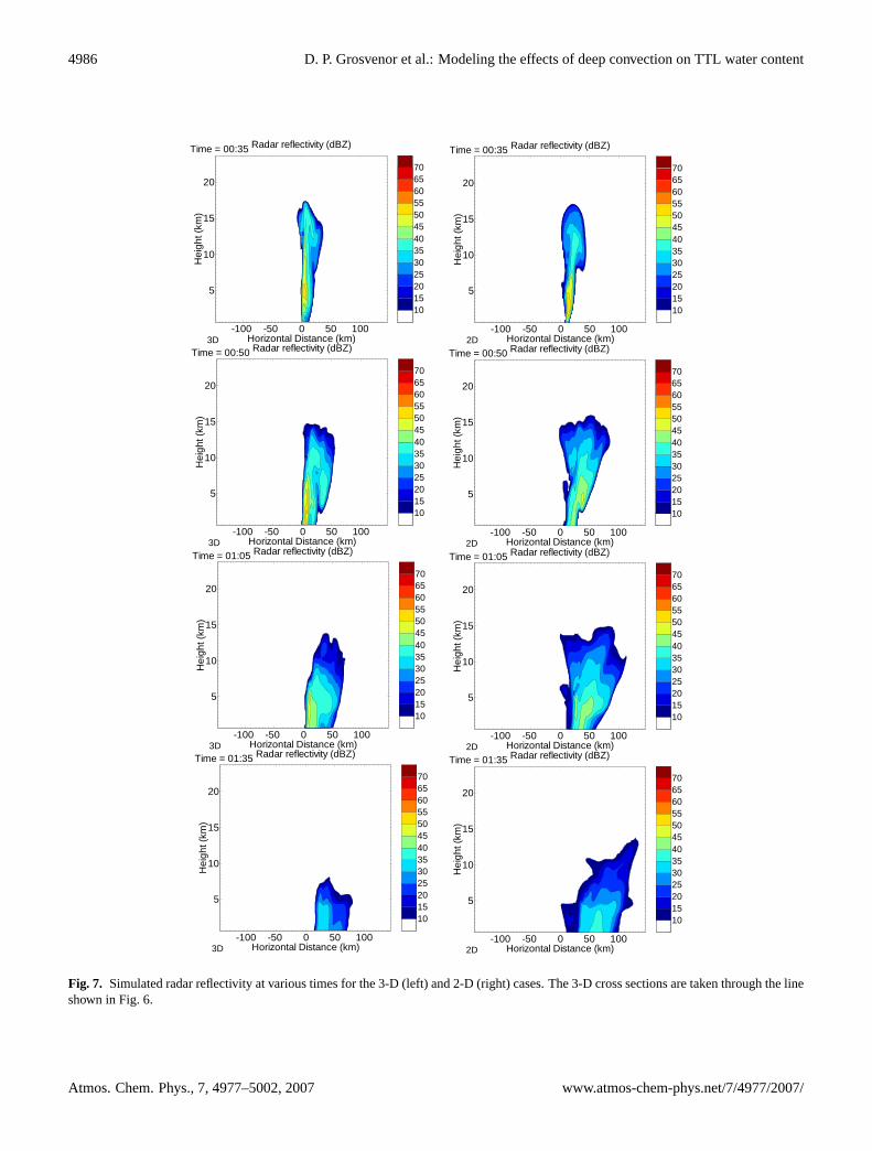
Figure6 is a horizontal cross-section of water vapour mix-ing ratio through the simulated 3-D cloud at 16.5 km and00:35, to give an idea of the location of the overshoot in themodel domain. This height is already above the tropopauseof the simulation environment and hence is likely to be withinthe TTL region. The effects on the water vapour are dis-cussed shortly, but first of all the simulated radar reflectivi-ties of a cross-section (dotted line in Fig.6) through the cloudare examined and compared to the 2-D case in order to ex-amine the general cloud features throughout the troposphere(Fig. 7).
The radar reflectivities, calculated every 5 min, show thatthe initial stages of the overshoot were more vigorous andreached higher altitudes in the 3-D case compared to the 2-Done, despite the same heating and moistening rates being ap-plied. For example, the 35 dBZ contour has reached up to justunder 17 km by 00:35 in the 3-D case, whereas it was onlyat ∼13 km in the 2-D case. In addition, the 40 dBZ reflec-tivity contour reached 15.1 km in one of the samples of thesimulated cloud reflectivity in the 3-D case, which were cal-culated every 5 min. By contrast, the 40 dBZ contour of the2-D case reached a maximum height of only 9.7 km. This in-dicates increased flux of larger ice hydrometeors in the 3-Dcase compared to that of the 2-D case. After this time, the2-D and 3-D cases show qualitatively similar clouds in termsof shapes and sizes, although in general the 2-D cloud was alittle wider than that in the 3-D simulation. This is especiallyapparent for the last time shown, where the 2-D cloud alsoextended up to higher altitudes. The width of the clouds dur-ing the growth and decay phases was generally similar to thesizes of clouds observed by the IPMet radar suggesting thatthe warm and moist bubble used was producing a cloud of arealistic size.
In the 3-D case, the contours near 17 km at 00:35 are veryclosely spaced so that the 10 dBZ contour is also close tothis height, as it is in the 2-D case. The radar statistics inTable 2 show that 124 cells (1.22% of 10 198 cell tracks)had maximum echo tops of≥17 km, clearly overshooting thetropopause, which was generally around 16 km during theexperimental period (Pommereau et al., 2007). Even thoughthe majority of the clouds that overshot the tropopause dur-ing the campaign did not have 40 dBZ echo tops as high asthose simulated in the 3-D case, they may still have had acomparable impact on the TTL region since they are stilllikely to have transported a significant enough amount of ice
Atmos. Chem. Phys., 7, 4977–5002, 2007 www.atmos-chem-phys.net/7/4977/2007/
D. P. Grosvenor et al.: Modeling the effects of deep convection on TTL water content 4985
Time = 00:35Time = 00:35
Fig. 6. Horizontal cross-sections at a height of 16.5 km of the water vapour mixing ratio at 35 min of simulation time for the 3-D case. Thedotted line represents the location of vertical cross-section shown in the following figures.
to potentially have had an impact on the low water content ofthe TTL. Radar reflectivities of up to 54–55 dBZ were sim-ulated in the interior of the cloud, which matched the maxi-mum observed at similar heights by the IPMet radar on thisday (54 dBZ).
A comparison of the simulated storm structures with radarobservations from this day yielded a reasonable agreement,as demonstrated in the vertical cross-section in Fig.5. Thehorizontal and vertical extents of the cell, selected from thestorm complex, are approximately the same magnitude as inthe simulation, even including the distribution of the higherradar reflectivities (cell core).
The maximum updraught speeds of the clouds show sig-nificant variation between the 2-D and 3-D cases with theabsolute maximum being 21 m s−1 at an altitude of 6.7 kmfor the former and 50 m s−1 at 12.5 km in the latter case. Theincreased vigour of the 3-D case relative to the 2-D one sug-gests that some of the differences in the behaviour of the twoovershooting clouds in the TTL that will be shown here, maybe due to the increased mass flux and ice transport of the 3-Dcase. Further tests with less vigorous 3-D clouds are there-fore examined later in order to determine whether or not thisis the case.
3.1.2 The effect on TTL water content during the simula-tion
Figure6 demonstrates that in the 3-D case the water vapourcontent at 16.5 km has been depleted significantly below theinitial environmental value through cold temperature ice de-
position. As well as the depleted vapour air formed in thecore of the overshoot, though, considerable vapour increaseshave also occurred in the surrounding air, with values as highas 25 ppmv being reached. This time corresponds to thatwhen the minimum vapour mixing ratio was achieved in the3-D case (see Fig.10).
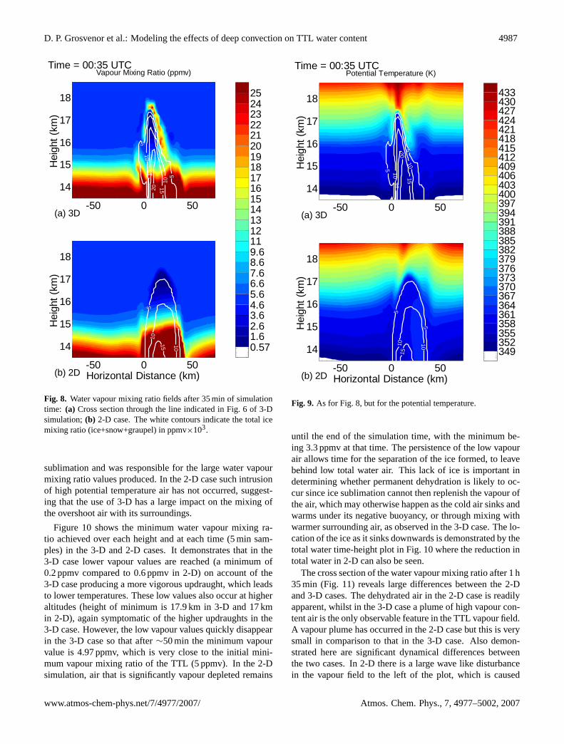
The vertical slices (Fig.8) show some similarities betweenthe 3-D and 2-D cases with a similar size of overshoot dis-turbance and similar minimum values produced in both cases(0.57 ppmv in 3-D and 0.62 ppmv in 2-D). The area coveredby the low vapour air is, however, significantly smaller inthe 3-D case and there is a large area of high vapour con-tent in the 3-D case that covers approximately half the areaof the dehydrated air seen in the 2-D simulation. In addi-tion, the boundary between the high vapour air below andthe depleted vapour above is much more irregular in the 3-Dcase, indicating that more mixing due to small scale motionsis occurring. Considerable amounts of ice were present inboth cases (see contours in Fig.8) in the same area as theovershoot air, allowing the possibility of significant moisten-ing through sublimation of this ice and making this a likelyexplanation for the high vapour air that was seen in the 3-Dcase.
This idea is supported by the potential temperature fieldfor these slices (Fig.9), which shows that in the 3-D casewarm high potential temperature air with values 380 to 400 Khas been dragged downwards below 16 km and into the over-shoot air from heights around 17 km. The location of this aircorresponds to the area of high water vapour described aboveand suggests that the warming due to its presence caused ice
www.atmos-chem-phys.net/7/4977/2007/ Atmos. Chem. Phys., 7, 4977–5002, 2007
4986 D. P. Grosvenor et al.: Modeling the effects of deep convection on TTL water content
10152025303540455055606570
-100 -50 0 50 100
5
10
15
20
Horizontal Distance (km)
Hei
ght (
km)
Radar reflectivity (dBZ)Time = 00:35
3D
10152025303540455055606570
-100 -50 0 50 100
5
10
15
20
Horizontal Distance (km)
Hei
ght (
km)
Radar reflectivity (dBZ)Time = 00:35
2D
10152025303540455055606570
-100 -50 0 50 100
5
10
15
20
Horizontal Distance (km)
Hei
ght (
km)
Radar reflectivity (dBZ)Time = 00:50
3D
10152025303540455055606570
-100 -50 0 50 100
5
10
15
20
Horizontal Distance (km)
Hei
ght (
km)
Radar reflectivity (dBZ)Time = 00:50
2D
10152025303540455055606570
-100 -50 0 50 100
5
10
15
20
Horizontal Distance (km)
Hei
ght (
km)
Radar reflectivity (dBZ)Time = 01:05
3D
10152025303540455055606570
-100 -50 0 50 100
5
10
15
20
Horizontal Distance (km)
Hei
ght (
km)
Radar reflectivity (dBZ)Time = 01:05
2D
10152025303540455055606570
-100 -50 0 50 100
5
10
15
20
Horizontal Distance (km)
Hei
ght (
km)
Radar reflectivity (dBZ)Time = 01:35
3D
10152025303540455055606570
-100 -50 0 50 100
5
10
15
20
Horizontal Distance (km)
Hei
ght (
km)
Radar reflectivity (dBZ)Time = 01:35
2D
10152025303540455055606570
-100 -50 0 50 100
5
10
15
20
Horizontal Distance (km)
Hei
ght (
km)
Radar reflectivity (dBZ)Time = 00:35
3D
10152025303540455055606570
-100 -50 0 50 100
5
10
15
20
Horizontal Distance (km)
Hei
ght (
km)
Radar reflectivity (dBZ)Time = 00:35
2D
10152025303540455055606570
-100 -50 0 50 100
5
10
15
20
Horizontal Distance (km)
Hei
ght (
km)
Radar reflectivity (dBZ)Time = 00:50
3D
10152025303540455055606570
-100 -50 0 50 100
5
10
15
20
Horizontal Distance (km)
Hei
ght (
km)
Radar reflectivity (dBZ)Time = 00:50
2D
10152025303540455055606570
-100 -50 0 50 100
5
10
15
20
Horizontal Distance (km)
Hei
ght (
km)
Radar reflectivity (dBZ)Time = 01:05
3D
10152025303540455055606570
-100 -50 0 50 100
5
10
15
20
Horizontal Distance (km)
Hei
ght (
km)
Radar reflectivity (dBZ)Time = 01:05
2D
10152025303540455055606570
-100 -50 0 50 100
5
10
15
20
Horizontal Distance (km)
Hei
ght (
km)
Radar reflectivity (dBZ)Time = 01:35
3D
10152025303540455055606570
-100 -50 0 50 100
5
10
15
20
Horizontal Distance (km)
Hei
ght (
km)
Radar reflectivity (dBZ)Time = 01:35
2D
Fig. 7. Simulated radar reflectivity at various times for the 3-D (left) and 2-D (right) cases. The 3-D cross sections are taken through the lineshown in Fig.6.
Atmos. Chem. Phys., 7, 4977–5002, 2007 www.atmos-chem-phys.net/7/4977/2007/
D. P. Grosvenor et al.: Modeling the effects of deep convection on TTL water content 4987
-50 0 50
14
15
16
17
18
Hei
ght (
km)
Vapour Mixing Ratio (ppmv)
5
5
10
10
15
1520
(a) 3D
Time = 00:35 UTC
0.571.62.63.64.65.66.67.68.69.6111213141516171819202122232425
-50 0 50
14
15
16
17
18
Horizontal Distance (km)
Hei
ght (
km)
5
5
10
1015
(b) 2D
Fig. 8. Water vapour mixing ratio fields after 35 min of simulationtime: (a) Cross section through the line indicated in Fig.6 of 3-Dsimulation;(b) 2-D case. The white contours indicate the total icemixing ratio (ice+snow+graupel) in ppmv×103.
sublimation and was responsible for the large water vapourmixing ratio values produced. In the 2-D case such intrusionof high potential temperature air has not occurred, suggest-ing that the use of 3-D has a large impact on the mixing ofthe overshoot air with its surroundings.
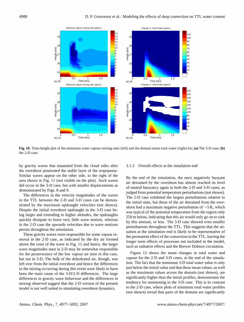
Figure 10 shows the minimum water vapour mixing ra-tio achieved over each height and at each time (5 min sam-ples) in the 3-D and 2-D cases. It demonstrates that in the3-D case lower vapour values are reached (a minimum of0.2 ppmv compared to 0.6 ppmv in 2-D) on account of the3-D case producing a more vigorous updraught, which leadsto lower temperatures. These low values also occur at higheraltitudes (height of minimum is 17.9 km in 3-D and 17 kmin 2-D), again symptomatic of the higher updraughts in the3-D case. However, the low vapour values quickly disappearin the 3-D case so that after∼50 min the minimum vapourvalue is 4.97 ppmv, which is very close to the initial mini-mum vapour mixing ratio of the TTL (5 ppmv). In the 2-Dsimulation, air that is significantly vapour depleted remains
-50 0 50
14
15
16
17
18
Hei
ght (
km)
Potential Temperature (K)
5
5
10
10
15
1520
(a) 3D
Time = 00:35 UTC
349352355358361364367370373376379382385388391394397400403406409412415418421424427430433
-50 0 50
14
15
16
17
18
Horizontal Distance (km)
Hei
ght (
km)
5
5
10 10
15
(b) 2D
Fig. 9. As for Fig.8, but for the potential temperature.
until the end of the simulation time, with the minimum be-ing 3.3 ppmv at that time. The persistence of the low vapourair allows time for the separation of the ice formed, to leavebehind low total water air. This lack of ice is important indetermining whether permanent dehydration is likely to oc-cur since ice sublimation cannot then replenish the vapour ofthe air, which may otherwise happen as the cold air sinks andwarms under its negative buoyancy, or through mixing withwarmer surrounding air, as observed in the 3-D case. The lo-cation of the ice as it sinks downwards is demonstrated by thetotal water time-height plot in Fig.10where the reduction intotal water in 2-D can also be seen.
The cross section of the water vapour mixing ratio after 1 h35 min (Fig.11) reveals large differences between the 2-Dand 3-D cases. The dehydrated air in the 2-D case is readilyapparent, whilst in the 3-D case a plume of high vapour con-tent air is the only observable feature in the TTL vapour field.A vapour plume has occurred in the 2-D case but this is verysmall in comparison to that in the 3-D case. Also demon-strated here are significant dynamical differences betweenthe two cases. In 2-D there is a large wave like disturbancein the vapour field to the left of the plot, which is caused
www.atmos-chem-phys.net/7/4977/2007/ Atmos. Chem. Phys., 7, 4977–5002, 2007
4988 D. P. Grosvenor et al.: Modeling the effects of deep convection on TTL water content
020406080100120140160180200220
0 0.5 1 1.5
15
16
17
18
19
Time (hrs)
Hei
ght (
km)
Change in Total Water (ppmv)
(b) 2D
0102030405060708090100110
0 0.5 1 1.5
15
16
17
18
19
Time (hrs)
Hei
ght (
km)
Change in Total Water (ppmv)
(a) 3D
123456789101112131415
0 0.5 1 1.5
15
16
17
18
19
Time (hrs)
Hei
ght (
km)
Minimum vapour mixing ratio (ppmv)
(b) 2D
123456789101112131415
0 0.5 1 1.5
15
16
17
18
19
Time (hrs)
Hei
ght (
km)
Minimum vapour mixing ratio (ppmv)
(a) 3D
Fig. 10.Time-height plot of the minimum water vapour mixing ratio (left) and the domain mean total water (right) for;(a) The 3-D case;(b)the 2-D case.
by gravity waves that emanated from the cloud sides afterthe overshoot penetrated the stable layer of the tropopause.Similar waves appear on the other side, to the right of thearea shown in Fig.11 (not visible on the plot). Such wavesdid occur in the 3-D case, but with smaller displacements asdemonstrated by Figs.8 and9.
The differences in the velocity magnitudes of the wavesin the TTL between the 2-D and 3-D cases can be demon-strated by the maximum updraught velocities (not shown).Despite the initial overshoot updraught in the 3-D case be-ing larger and extending to higher altitudes, the updraughtsquickly dissipate to leave very little wave motion, whereasin the 2-D case the upwards velocities due to wave motionspersist throughout the simulation.
These gravity waves were responsible for some vapour re-moval in the 2-D case, as indicated by the dry air formedabove the crest of the wave in Fig.11 and hence, the largerwave magnitudes seen in 2-D may be somewhat responsiblefor the perseverance of the low vapour air seen in this case,but not in 3-D. The bulk of the dehydrated air, though, wasleft over from the initial overshoot and hence the differencesin the mixing occurring during this event were likely to havebeen the main cause of the 3-D/2-D differences. The largedifferences in gravity wave behaviour and the differences inmixing observed suggest that the 2-D version of the presentmodel is not well suited to simulating overshoot dynamics.
3.1.3 Overall effects at the simulation end
By the end of the simulation, the once negatively buoyantair detrained by the overshoot has almost reached its levelof neutral buoyancy again in both the 2-D and 3-D cases, asjudged from potential temperature perturbations (not shown).The 2-D case exhibited the largest perturbations relative tothe initial state, but those of the air detrained from the over-shoot had a maximum negative perturbation of∼5 K, whichwas typical of the potential temperature from the region only250 m below, indicating that this air would only go on to sinkby this amount, or less. The 3-D case showed even smallerperturbations throughout the TTL. This suggests that the sit-uation at the simulation end is likely to be representative ofthe permanent effect of the convection in the TTL, barring thelonger term effects of processes not included in the model,such as radiative effects and the Brewer Dobson circulation.
Figure 12 shows the mean changes in total water andvapour for the 2-D and 3-D cases, at the end of the simula-tion. The fact that the minimum 3-D total water value is onlyjust below the initial value and that these mean values, as wellas the maximum values across the domain (not shown), aresignificantly higher than the initial profiles, demonstrates thetendency for moistening in the 3-D case. This is in contrastto the 2-D case, where plots of minimum total water profiles(not shown) reveal that parts of the domain are significantly
Atmos. Chem. Phys., 7, 4977–5002, 2007 www.atmos-chem-phys.net/7/4977/2007/
D. P. Grosvenor et al.: Modeling the effects of deep convection on TTL water content 4989
-100 -50 0 50 100
14
15
16
17
18
Hei
ght (
km)
Vapour Mixing Ratio (ppmv)
(a) 3D
Time = 01:35 UTC
2345678910111213141516171819202122232425
-100 -50 0 50 100
14
15
16
17
18
Horizontal Distance (km)
Hei
ght (
km)
(b) 2D
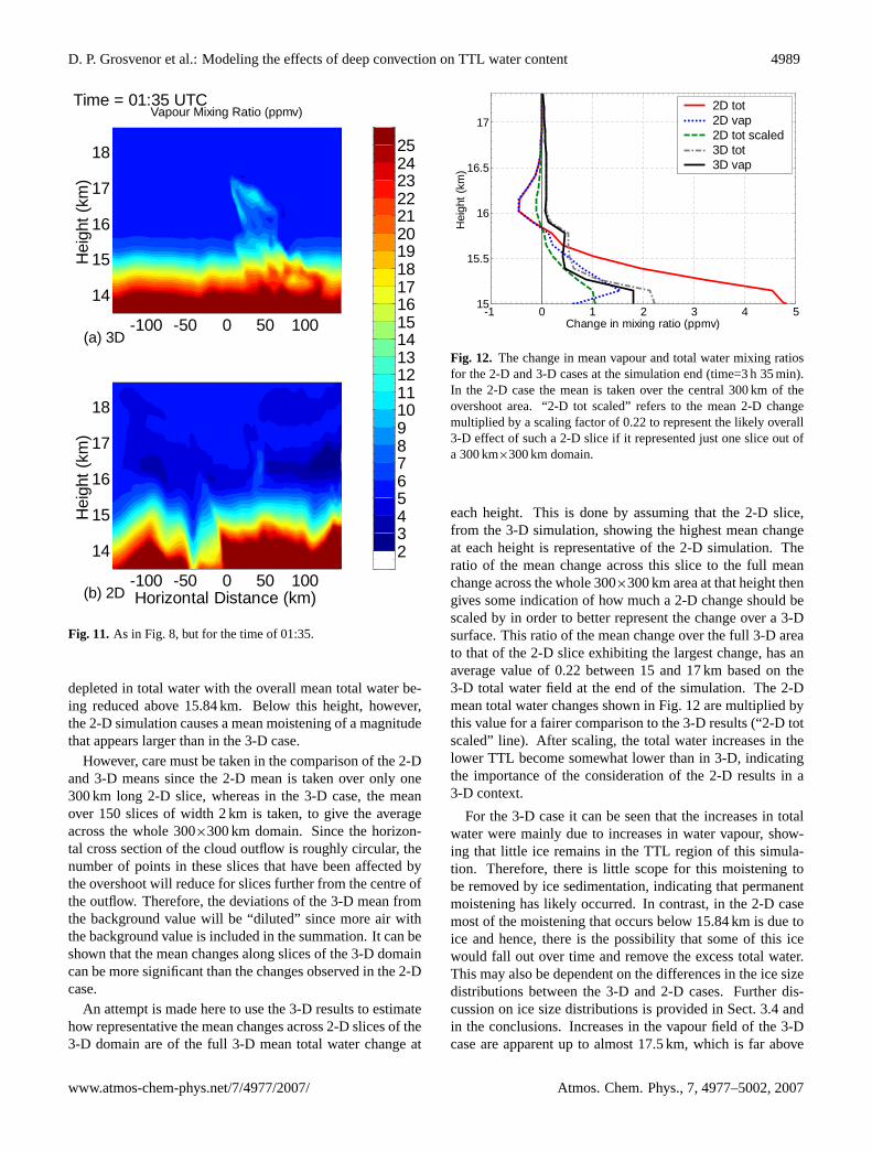
Fig. 11. As in Fig.8, but for the time of 01:35.
depleted in total water with the overall mean total water be-ing reduced above 15.84 km. Below this height, however,the 2-D simulation causes a mean moistening of a magnitudethat appears larger than in the 3-D case.
However, care must be taken in the comparison of the 2-Dand 3-D means since the 2-D mean is taken over only one300 km long 2-D slice, whereas in the 3-D case, the meanover 150 slices of width 2 km is taken, to give the averageacross the whole 300×300 km domain. Since the horizon-tal cross section of the cloud outflow is roughly circular, thenumber of points in these slices that have been affected bythe overshoot will reduce for slices further from the centre ofthe outflow. Therefore, the deviations of the 3-D mean fromthe background value will be “diluted” since more air withthe background value is included in the summation. It can beshown that the mean changes along slices of the 3-D domaincan be more significant than the changes observed in the 2-Dcase.
An attempt is made here to use the 3-D results to estimatehow representative the mean changes across 2-D slices of the3-D domain are of the full 3-D mean total water change at
-1 0 1 2 3 4 515
15.5
16
16.5
17
Change in mixing ratio (ppmv)
Hei
ght (
km)
2D tot2D vap2D tot scaled3D tot3D vap
Fig. 12. The change in mean vapour and total water mixing ratiosfor the 2-D and 3-D cases at the simulation end (time=3 h 35 min).In the 2-D case the mean is taken over the central 300 km of theovershoot area. “2-D tot scaled” refers to the mean 2-D changemultiplied by a scaling factor of 0.22 to represent the likely overall3-D effect of such a 2-D slice if it represented just one slice out ofa 300 km×300 km domain.
each height. This is done by assuming that the 2-D slice,from the 3-D simulation, showing the highest mean changeat each height is representative of the 2-D simulation. Theratio of the mean change across this slice to the full meanchange across the whole 300×300 km area at that height thengives some indication of how much a 2-D change should bescaled by in order to better represent the change over a 3-Dsurface. This ratio of the mean change over the full 3-D areato that of the 2-D slice exhibiting the largest change, has anaverage value of 0.22 between 15 and 17 km based on the3-D total water field at the end of the simulation. The 2-Dmean total water changes shown in Fig.12 are multiplied bythis value for a fairer comparison to the 3-D results (“2-D totscaled” line). After scaling, the total water increases in thelower TTL become somewhat lower than in 3-D, indicatingthe importance of the consideration of the 2-D results in a3-D context.
For the 3-D case it can be seen that the increases in totalwater were mainly due to increases in water vapour, show-ing that little ice remains in the TTL region of this simula-tion. Therefore, there is little scope for this moistening tobe removed by ice sedimentation, indicating that permanentmoistening has likely occurred. In contrast, in the 2-D casemost of the moistening that occurs below 15.84 km is due toice and hence, there is the possibility that some of this icewould fall out over time and remove the excess total water.This may also be dependent on the differences in the ice sizedistributions between the 3-D and 2-D cases. Further dis-cussion on ice size distributions is provided in Sect. 3.4 andin the conclusions. Increases in the vapour field of the 3-Dcase are apparent up to almost 17.5 km, which is far above
www.atmos-chem-phys.net/7/4977/2007/ Atmos. Chem. Phys., 7, 4977–5002, 2007
4990 D. P. Grosvenor et al.: Modeling the effects of deep convection on TTL water content
10152025303540455055606570
-20 0 20
5
10
15
20
Horizontal Distance (km)
Hei
ght (
km)
Radar reflectivity (dBZ)Time = 00:30
(a) 3D
10152025303540455055606570
-20 0 20
5
10
15
20
Horizontal Distance (km)
Hei
ght (
km)
Radar reflectivity (dBZ)Time = 00:35
(b) 3D-med
10152025303540455055606570
-20 0 20
5
10
15
20
Horizontal Distance (km)
Hei
ght (
km)
Radar reflectivity (dBZ)Time = 00:40
(c) 3D-weak
10152025303540455055606570
-20 0 20
5
10
15
20
Horizontal Distance (km)
Hei
ght (
km)
Radar reflectivity (dBZ)Time = 00:30
(a) 3D
10152025303540455055606570
-20 0 20
5
10
15
20
Horizontal Distance (km)
Hei
ght (
km)
Radar reflectivity (dBZ)Time = 00:35
(b) 3D-med
10152025303540455055606570
-20 0 20
5
10
15
20
Horizontal Distance (km)
Hei
ght (
km)
Radar reflectivity (dBZ)Time = 00:40
(c) 3D-weak
Fig. 13.Cross sections of the simulated radar reflectivity of the 3-Dcases of various strengths taken though the slice inidicated in Fig.6.
the tropopause (15.9 km), suggesting that direct moisteningof the stratosphere has occurred here, although the increasesat these high altitudes are much lower than those below thetropopause.
3.2 Weaker 3-D cases
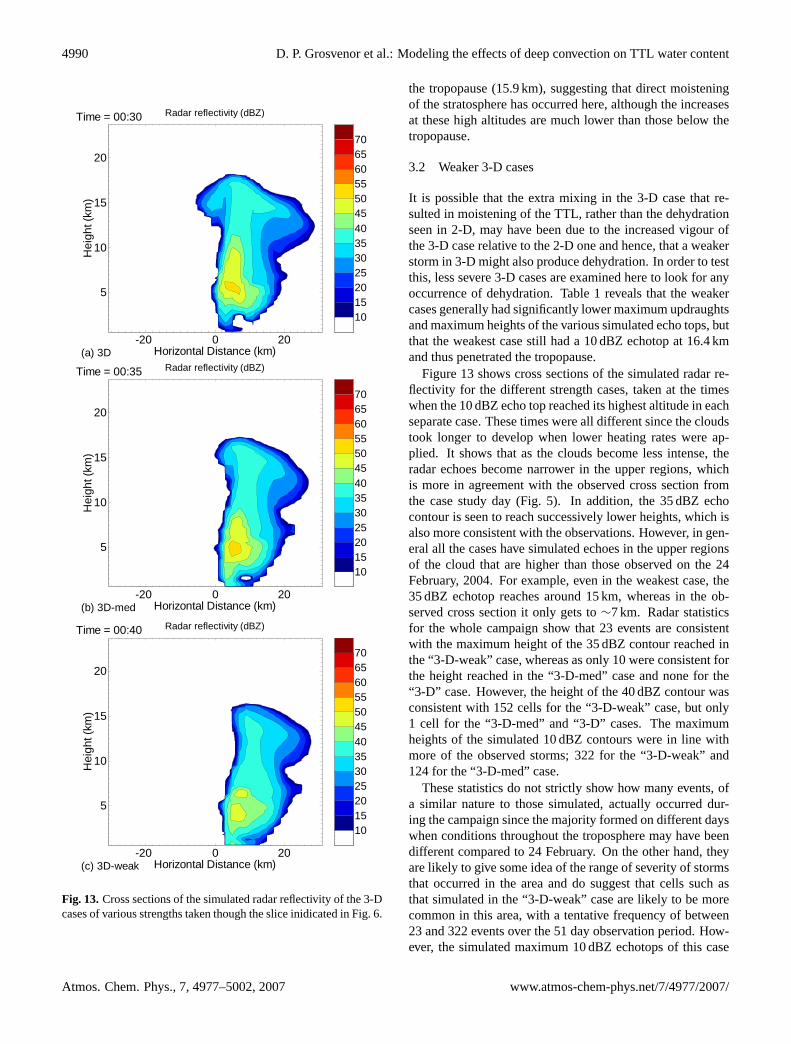
It is possible that the extra mixing in the 3-D case that re-sulted in moistening of the TTL, rather than the dehydrationseen in 2-D, may have been due to the increased vigour ofthe 3-D case relative to the 2-D one and hence, that a weakerstorm in 3-D might also produce dehydration. In order to testthis, less severe 3-D cases are examined here to look for anyoccurrence of dehydration. Table 1 reveals that the weakercases generally had significantly lower maximum updraughtsand maximum heights of the various simulated echo tops, butthat the weakest case still had a 10 dBZ echotop at 16.4 kmand thus penetrated the tropopause.
Figure13 shows cross sections of the simulated radar re-flectivity for the different strength cases, taken at the timeswhen the 10 dBZ echo top reached its highest altitude in eachseparate case. These times were all different since the cloudstook longer to develop when lower heating rates were ap-plied. It shows that as the clouds become less intense, theradar echoes become narrower in the upper regions, whichis more in agreement with the observed cross section fromthe case study day (Fig.5). In addition, the 35 dBZ echocontour is seen to reach successively lower heights, which isalso more consistent with the observations. However, in gen-eral all the cases have simulated echoes in the upper regionsof the cloud that are higher than those observed on the 24February, 2004. For example, even in the weakest case, the35 dBZ echotop reaches around 15 km, whereas in the ob-served cross section it only gets to∼7 km. Radar statisticsfor the whole campaign show that 23 events are consistentwith the maximum height of the 35 dBZ contour reached inthe “3-D-weak” case, whereas as only 10 were consistent forthe height reached in the “3-D-med” case and none for the“3-D” case. However, the height of the 40 dBZ contour wasconsistent with 152 cells for the “3-D-weak” case, but only1 cell for the “3-D-med” and “3-D” cases. The maximumheights of the simulated 10 dBZ contours were in line withmore of the observed storms; 322 for the “3-D-weak” and124 for the “3-D-med” case.
These statistics do not strictly show how many events, ofa similar nature to those simulated, actually occurred dur-ing the campaign since the majority formed on different dayswhen conditions throughout the troposphere may have beendifferent compared to 24 February. On the other hand, theyare likely to give some idea of the range of severity of stormsthat occurred in the area and do suggest that cells such asthat simulated in the “3-D-weak” case are likely to be morecommon in this area, with a tentative frequency of between23 and 322 events over the 51 day observation period. How-ever, the simulated maximum 10 dBZ echotops of this case
Atmos. Chem. Phys., 7, 4977–5002, 2007 www.atmos-chem-phys.net/7/4977/2007/
D. P. Grosvenor et al.: Modeling the effects of deep convection on TTL water content 4991
(16.4 km) and even of that of the strongest case (18.2 km) areconsiderably lower than that observed for a significant num-ber of the observed cells, suggesting that some of the realclouds reached higher than those simulated, and that it maybe inaccuracies in the model microphysics or the treatmentused to calculate the radar reflectivites from the model fieldsthat are leading to artificially high simulated radar reflectivi-ties.
Most of the simulated reflectivity in the upper regions canbe shown to be due to the graupel hydrometeor since the re-flectivity is much larger for bigger particles. Such particlesare likely to fall out quickly from the overshooting cloud andwould evaporate more slowly upon mixing with stratosphericair. Therefore, their presence might indicate an underestima-tion of the amount of moistening that would occur in reality,assuming that the total mass of water transported to the uppercloud is accurate. If this is the case, it may be that the overallheight reached by the cloud, which is perhaps better capturedby the 10 dBZ echotop, is more representative for estimatingthe number of real events that are likely to have had an effecton the TTL water content that is similar to those simulated.Then, comparisons of the high reflectivity contours may notbe useful. On the other hand, increased amounts of graupelcould indicate that too much water mass is being transportedupwards by the cloud, perhaps due to a lack of removal byprecipitation lower down or a lack on entrainment of dry airinto the lower regions of the cloud caused by inaccuracies inthe model dynamics. Further simulations and comparisonsto observations are required to determine which is the case.
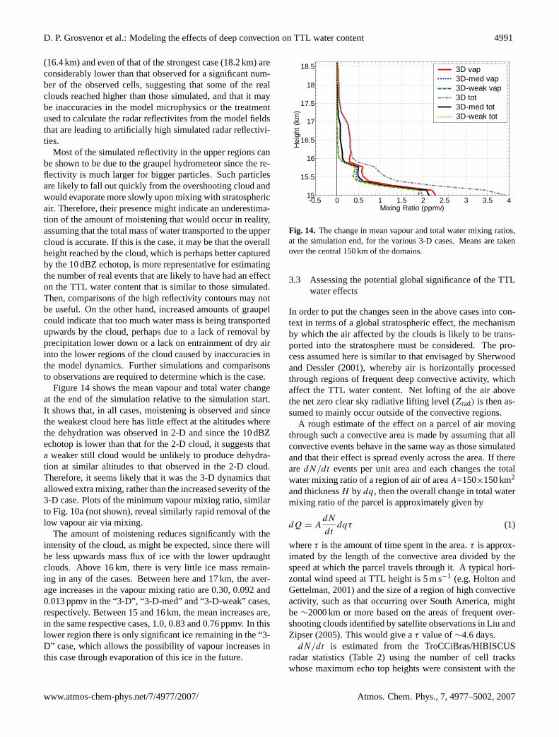
Figure14 shows the mean vapour and total water changeat the end of the simulation relative to the simulation start.It shows that, in all cases, moistening is observed and sincethe weakest cloud here has little effect at the altitudes wherethe dehydration was observed in 2-D and since the 10 dBZechotop is lower than that for the 2-D cloud, it suggests thata weaker still cloud would be unlikely to produce dehydra-tion at similar altitudes to that observed in the 2-D cloud.Therefore, it seems likely that it was the 3-D dynamics thatallowed extra mixing, rather than the increased severity of the3-D case. Plots of the minimum vapour mixing ratio, similarto Fig.10a (not shown), reveal similarly rapid removal of thelow vapour air via mixing.
The amount of moistening reduces significantly with theintensity of the cloud, as might be expected, since there willbe less upwards mass flux of ice with the lower updraughtclouds. Above 16 km, there is very little ice mass remain-ing in any of the cases. Between here and 17 km, the aver-age increases in the vapour mixing ratio are 0.30, 0.092 and0.013 ppmv in the “3-D”, “3-D-med” and “3-D-weak” cases,respectively. Between 15 and 16 km, the mean increases are,in the same respective cases, 1.0, 0.83 and 0.76 ppmv. In thislower region there is only significant ice remaining in the “3-D” case, which allows the possibility of vapour increases inthis case through evaporation of this ice in the future.
-0.5 0 0.5 1 1.5 2 2.5 3 3.5 415
15.5
16
16.5
17
17.5
18
18.5
Mixing Ratio (ppmv)
Hei
ght (
km)
3D vap3D-med vap3D-weak vap3D tot3D-med tot3D-weak tot
Fig. 14. The change in mean vapour and total water mixing ratios,at the simulation end, for the various 3-D cases. Means are takenover the central 150 km of the domains.
3.3 Assessing the potential global significance of the TTLwater effects
In order to put the changes seen in the above cases into con-text in terms of a global stratospheric effect, the mechanismby which the air affected by the clouds is likely to be trans-ported into the stratosphere must be considered. The pro-cess assumed here is similar to that envisaged by Sherwoodand Dessler (2001), whereby air is horizontally processedthrough regions of frequent deep convective activity, whichaffect the TTL water content. Net lofting of the air abovethe net zero clear sky radiative lifting level (Zrad) is then as-sumed to mainly occur outside of the convective regions.
A rough estimate of the effect on a parcel of air movingthrough such a convective area is made by assuming that allconvective events behave in the same way as those simulatedand that their effect is spread evenly across the area. If therearedN/dt events per unit area and each changes the totalwater mixing ratio of a region of air of areaA=150×150 km2
and thicknessH by dq, then the overall change in total watermixing ratio of the parcel is approximately given by
dQ = AdN
dtdqτ (1)
whereτ is the amount of time spent in the area.τ is approx-imated by the length of the convective area divided by thespeed at which the parcel travels through it. A typical hori-zontal wind speed at TTL height is 5 m s−1 (e.g. Holton andGettelman, 2001) and the size of a region of high convectiveactivity, such as that occurring over South America, mightbe ∼2000 km or more based on the areas of frequent over-shooting clouds identified by satellite observations in Liu andZipser (2005). This would give aτ value of∼4.6 days.
dN/dt is estimated from the TroCCiBras/HIBISCUSradar statistics (Table 2) using the number of cell trackswhose maximum echo top heights were consistent with the
www.atmos-chem-phys.net/7/4977/2007/ Atmos. Chem. Phys., 7, 4977–5002, 2007
4992 D. P. Grosvenor et al.: Modeling the effects of deep convection on TTL water content
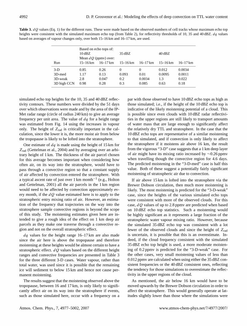
Table 3. dQ values (Eq. 1) for the different runs. These were made based on the observed numbers of cell tracks whose maximum echo topheights were consistent with the simulated maximum echo top (from Table 2), for reflectivity thresholds of 10, 35 and 40 dBZ.dq valuesbased on averages of vapour changes only, over both 15–16 km and 16–17 km, are used.
Based on echo tops of:10 dBZ 35 dBZ 40 dBZMeandQ (ppmv) over:
Run 15–16 km 16–17 km 15–16 km 16–17 km 15–16 km 16–17 km
3-D 0.85 0.26 0 0 0.012 0.00343D-med 1.17 0.13 0.093 0.01 0.0095 0.00113D-weak 2.8 0.047 0.2 0.0034 1.3 0.0223D high CCN 0.98 0.28 0.3 0.085 0.63 0.18
simulated echo top heights for the 10, 35 and 40 dBZ reflec-tivity contours. These numbers were divided by the 51 daysover which observations were made and by the area of the IP-Met radar range (circle of radius 240 km) to give an averagefrequency per unit area. The value ofdq for a height rangewas estimated from Fig.14 using the increases in vapouronly. The height ofZrad is critically important in the cal-culation, since the lower it is, the more moist air from belowthe tropopause is likely to be lofted into the stratosphere.
One estimate ofdq is made using the height of 15 km forZrad (Gettelman et al., 2004) and by averaging over an arbi-trary height of 1 km. The thickness of the air parcel chosenfor this average becomes important when considering howoften air, on its way into the stratosphere, would have topass through a convective region so that a constant supplyof air affected by convection entered the stratosphere. Witha typical ascent rate of just over 1 km month−1 (e.g., Holtonand Gettelman, 2001) all the air parcels in the 1 km regionwould need to be affected by convection approximately ev-ery month, if thedQ value estimated here is to apply to thestratospheric entry mixing ratio of air. However, an estima-tion of the frequency that trajectories on the way into thestratosphere sample convective regions is beyond the scopeof this study. The moistening estimates given here are in-tended to give a rough idea of the effect on 1 km deep airparcels as they make one traverse through a convective re-gion and not on the overall stratospheric effect.
dq values for the height range 16–17 km are also madesince the air here is above the tropopause and thereforemoistening at these heights would be almost certain to have astratospheric effect.dQ values based on the different heightranges and convective frequencies are presented in Table 3for the three different 3-D cases. Water vapour, rather thantotal water, was used since it is possible that the remainingice will sediment to below 15 km and hence not cause per-manent moistening.
The results suggest that the moistening observed above thetropopause, between 16 and 17 km, is only likely to signifi-cantly affect air on its way into the stratosphere if events,such as those simulated here, occur with a frequency on a
par with those observed to have 10 dBZ echo tops as high asthose simulated; i.e., if the height of the 10 dBZ echo top isindicative of the likely moistening potential of a cloud. Thisis possible since even clouds with 10 dBZ radar reflectivi-ties in the upper regions are still likely to transport amountsof water mass that are large enough to significantly affectthe relatively dry TTL and stratosphere. In the case that the10 dBZ echo tops are representative of a similar moisteningto that simulated, and if convection is only likely to affectthe stratosphere if it moistens air above 16 km, the resultfrom the vigorous “3-D” case suggests that a 1 km deep layerof air might have its mixing ratio increased by∼0.26 ppmvwhen travelling though the convective region for 4.6 days.The predicted moistening in the “3-D-med” case is half thisvalue. Both of these suggest a potentially fairly significantmoistening of stratospheric air due to convection.
If air above 15 km is lofted into the stratosphere via theBrewer Dobson circulation, then much more moistening islikely. The most moistening is predicted for the “3-D-weak”case, since the heights of the various simulated echo topswere consistent with more of the observed clouds. For thiscase,dQ values of up to 2.8 ppmv are predicted when basedon 10 dBZ echo top statistics. Such a moistening wouldbe highly significant as it represents a large fraction of thestratospheric water vapour mixing ratio. However, becausethe simulated 35 dBZ echo top was consistent with a lotfewer of the observed clouds and since the height ofZradis uncertain, it is possible that this is an overestimate. In-deed, if the cloud frequency consistent with the simulated35 dBZ echo top height is used, a more moderate moisten-ing of 0.2 ppmv is predicted for the “3-D-weak” case. Forthe other cases, very small moistening values of less than0.012 ppmv are calculated when using either the 35 dBZ con-sistent frequencies or the 40 dBZ consistent ones, reflectingthe tendency for those simulations to overestimate the reflec-tivity in the upper regions of the cloud.
As mentioned, the air below 16 km would have to bemoved upwards by the Brewer Dobson circulation in order toaffect the stratosphere. This would generally operate at lat-itudes slightly lower than those where the simulations were
Atmos. Chem. Phys., 7, 4977–5002, 2007 www.atmos-chem-phys.net/7/4977/2007/
D. P. Grosvenor et al.: Modeling the effects of deep convection on TTL water content 4993
based, hence meaning that the air would have to travel equa-torwards before this was possible. Even if this does occur theair is likely to be below the local cold point and hence willhave to ascend through it to reach the stratosphere. This mayresult in dehydration of the moistened air and may thereforereduce the impact of the convective moistening on the strato-sphere for the air below the Bauru tropopause. However,since air at the cold point can often be sub-saturated there ispotential for moisture transported up to below the cold pointto play some role in increasing the moisture content of airentering the stratosphere, relative to that which would havecrossed the cold point had the convection not occurred.
Overall, the results suggest that the issues of whether airbelow the tropopause is likely to affect the stratosphere lateron and whether clouds with similar 10 dBZ echo tops to thosesimulated will have a similar stratospheric moistening to thatpredicted by the simulations, despite generally having lowerecho tops for the higher reflectivity contours, will be key inpredicting the stratospheric effect of convective clouds basedon these and other CRM simulations.
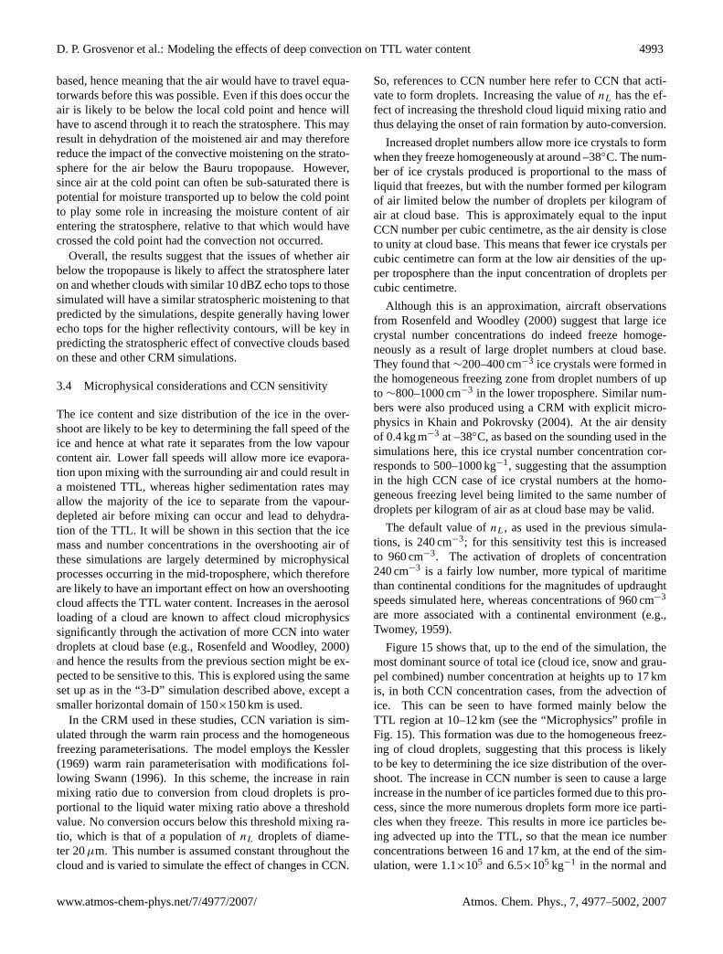
3.4 Microphysical considerations and CCN sensitivity
The ice content and size distribution of the ice in the over-shoot are likely to be key to determining the fall speed of theice and hence at what rate it separates from the low vapourcontent air. Lower fall speeds will allow more ice evapora-tion upon mixing with the surrounding air and could result ina moistened TTL, whereas higher sedimentation rates mayallow the majority of the ice to separate from the vapour-depleted air before mixing can occur and lead to dehydra-tion of the TTL. It will be shown in this section that the icemass and number concentrations in the overshooting air ofthese simulations are largely determined by microphysicalprocesses occurring in the mid-troposphere, which thereforeare likely to have an important effect on how an overshootingcloud affects the TTL water content. Increases in the aerosolloading of a cloud are known to affect cloud microphysicssignificantly through the activation of more CCN into waterdroplets at cloud base (e.g., Rosenfeld and Woodley, 2000)and hence the results from the previous section might be ex-pected to be sensitive to this. This is explored using the sameset up as in the “3-D” simulation described above, except asmaller horizontal domain of 150×150 km is used.
In the CRM used in these studies, CCN variation is sim-ulated through the warm rain process and the homogeneousfreezing parameterisations. The model employs the Kessler(1969) warm rain parameterisation with modifications fol-lowing Swann (1996). In this scheme, the increase in rainmixing ratio due to conversion from cloud droplets is pro-portional to the liquid water mixing ratio above a thresholdvalue. No conversion occurs below this threshold mixing ra-tio, which is that of a population ofnL droplets of diame-ter 20µm. This number is assumed constant throughout thecloud and is varied to simulate the effect of changes in CCN.
So, references to CCN number here refer to CCN that acti-vate to form droplets. Increasing the value ofnL has the ef-fect of increasing the threshold cloud liquid mixing ratio andthus delaying the onset of rain formation by auto-conversion.
Increased droplet numbers allow more ice crystals to formwhen they freeze homogeneously at around –38◦C. The num-ber of ice crystals produced is proportional to the mass ofliquid that freezes, but with the number formed per kilogramof air limited below the number of droplets per kilogram ofair at cloud base. This is approximately equal to the inputCCN number per cubic centimetre, as the air density is closeto unity at cloud base. This means that fewer ice crystals percubic centimetre can form at the low air densities of the up-per troposphere than the input concentration of droplets percubic centimetre.
Although this is an approximation, aircraft observationsfrom Rosenfeld and Woodley (2000) suggest that large icecrystal number concentrations do indeed freeze homoge-neously as a result of large droplet numbers at cloud base.They found that∼200–400 cm−3 ice crystals were formed inthe homogeneous freezing zone from droplet numbers of upto ∼800–1000 cm−3 in the lower troposphere. Similar num-bers were also produced using a CRM with explicit micro-physics in Khain and Pokrovsky (2004). At the air densityof 0.4 kg m−3 at –38◦C, as based on the sounding used in thesimulations here, this ice crystal number concentration cor-responds to 500–1000 kg−1, suggesting that the assumptionin the high CCN case of ice crystal numbers at the homo-geneous freezing level being limited to the same number ofdroplets per kilogram of air as at cloud base may be valid.
The default value ofnL, as used in the previous simula-tions, is 240 cm−3; for this sensitivity test this is increasedto 960 cm−3. The activation of droplets of concentration240 cm−3 is a fairly low number, more typical of maritimethan continental conditions for the magnitudes of updraughtspeeds simulated here, whereas concentrations of 960 cm−3
are more associated with a continental environment (e.g.,Twomey, 1959).
Figure15 shows that, up to the end of the simulation, themost dominant source of total ice (cloud ice, snow and grau-pel combined) number concentration at heights up to 17 kmis, in both CCN concentration cases, from the advection ofice. This can be seen to have formed mainly below theTTL region at 10–12 km (see the “Microphysics” profile inFig. 15). This formation was due to the homogeneous freez-ing of cloud droplets, suggesting that this process is likelyto be key to determining the ice size distribution of the over-shoot. The increase in CCN number is seen to cause a largeincrease in the number of ice particles formed due to this pro-cess, since the more numerous droplets form more ice parti-cles when they freeze. This results in more ice particles be-ing advected up into the TTL, so that the mean ice numberconcentrations between 16 and 17 km, at the end of the sim-ulation, were 1.1×10⁵ and 6.5×10⁵ kg−1 in the normal and
www.atmos-chem-phys.net/7/4977/2007/ Atmos. Chem. Phys., 7, 4977–5002, 2007
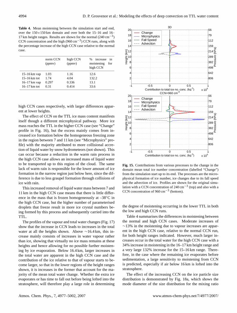
4994 D. P. Grosvenor et al.: Modeling the effects of deep convection on TTL water content
Table 4. Mean moistening between the simulation start and end,over the 150×150 km domain and over both the 15–16 and 16–17 km height ranges. Results are shown for the normal (240 cm−3)CCN concentration and the high (960 cm−3) CCN runs, along withthe percentage increase of the high CCN case relative to the normalcase.
norm CCN(ppmv)
high CCN(ppmv)
% increase inmoistening forhigh CCN
15–16 km vap 1.03 1.16 12.615–16 km tot 1.74 4.04 132.216–17 km vap 0.297 0.336 13.116–17 km tot 0.31 0.414 33.6
high CCN cases respectively, with larger differences appar-ent at lower heights.
The effect of CCN on the TTL ice mass content manifestsitself though a different microphysical pathway. More icemass reaches the TTL in the higher CCN case (see “Change”profile in Fig. 16), but the excess mainly comes from in-creased ice formation below the homogeneous freezing zonein the region between 7 and 11 km (see “Microphysics” pro-file) with the majority attributed to more collisional accre-tion of liquid water by snow hydrometeors (not shown). Thiscan occur because a reduction in the warm rain process inthe high CCN case allows an increased mass of liquid waterto be transported up to this region of the cloud. The samelack of warm rain is responsible for the lower amount of iceformation in the narrow region just below here, since the dif-ference is due to less graupel formation through collisions ofice with rain.
This increased removal of liquid water mass between 7 and11 km in the high CCN case means that there is little differ-ence in the mass that is frozen homogeneously at –38◦C inthe high CCN case, but the higher number of parameteriseddroplets that freeze result in more ice crystal numbers be-ing formed by this process and subsequently carried into theTTL.
The profiles of the vapour and total water changes (Fig.17)show that the increase in CCN leads to increases in the totalwater at all the heights shown. Above∼16.4 km, this in-crease mainly consists of increases in water vapour ratherthan ice, showing that virtually no ice mass remains at theseheights and hence allowing for no possible further moisten-ing by ice evaporation. Below 16.4 km, larger increases inthe total water are apparent in the high CCN case and thecontribution of the ice relative to that of vapour starts to be-come larger, so that in the lower regions of the height rangesshown, it is increases in the former that account for the ma-jority of the mean total water change. Whether the extra iceevaporates or has time to fall out before being lofted into thestratosphere, will therefore play a large role in determining
806
642
498
382
289
214
159
112
79
56
Pre
ssur
e (h
Pa)
-1 -0.5 0 0.5 1x 10⁸
2
4
6
8
10
12
14
16
18
20
Contribution to total ice no. conc. (kg-1)
Hei
ght (
km)
3D
ChangeMicrophysicsFall SpeedAdvection
806
642
498
382
289
214
159
112
79
56
Pre
ssur
e (h
Pa)
-1 -0.5 0 0.5 1x 10⁸
2
4
6
8
10
12
14
16
18
20
Contribution to total ice no. conc. (kg-1)
Hei
ght (
km)
CCN=960 cm-3
ChangeMicrophysicsFall SpeedAdvection
806
642
498
382
289
214
159
112
79
56
Pre
ssur
e (h
Pa)
-1 -0.5 0 0.5 1x 10⁸
2
4
6
8
10
12
14
16
18
20
Contribution to total ice no. conc. (kg-1)
Hei
ght (
km)
3D
ChangeMicrophysicsFall SpeedAdvection
806
642
498
382
289
214
159
112
79
56
Pre
ssur
e (h
Pa)
-1 -0.5 0 0.5 1x 10⁸
2
4
6
8
10
12
14
16
18
20
Contribution to total ice no. conc. (kg-1)
Hei
ght (
km)
CCN=960 cm-3
ChangeMicrophysicsFall SpeedAdvection
Fig. 15. Contributions from various processes to the change in thedomain mean total ice number concentration (labelled “Change”)from the simulation start up to its end. The processes are the micro-physical formation of ice number, ice changes due to its fall speedand the advection of ice. Profiles are shown for the original simu-lation with a CCN concentration of 240 cm−3 (top) and also with aCCN concentration of 960 cm−3 (bottom).
the degree of moistening occurring in the lower TTL in boththe low and high CCN runs.
Table 4 summarises the differences in moistening betweenthe normal and high CCN cases. Moderate increases of∼13% in the moistening due to vapour increases are appar-ent in the high CCN case, relative to the normal CCN run,for both height ranges indicated. However, much larger in-creases occur in the total water for the high CCN case with a34% increase in moistening in the 16–17 km height range anda very large 132% increase for the 15–16 km range. There-fore, in the case where the remaining ice evaporates beforesedimentation, a large sensitivity to moistening from CCNis predicted, especially if air below 16 km is lofted into thestratosphere.
The effect of the increasing CCN on the ice particle sizedistribution is demonstrated by Fig.18a, which shows themode diameter of the size distribution for the mixing ratio
Atmos. Chem. Phys., 7, 4977–5002, 2007 www.atmos-chem-phys.net/7/4977/2007/
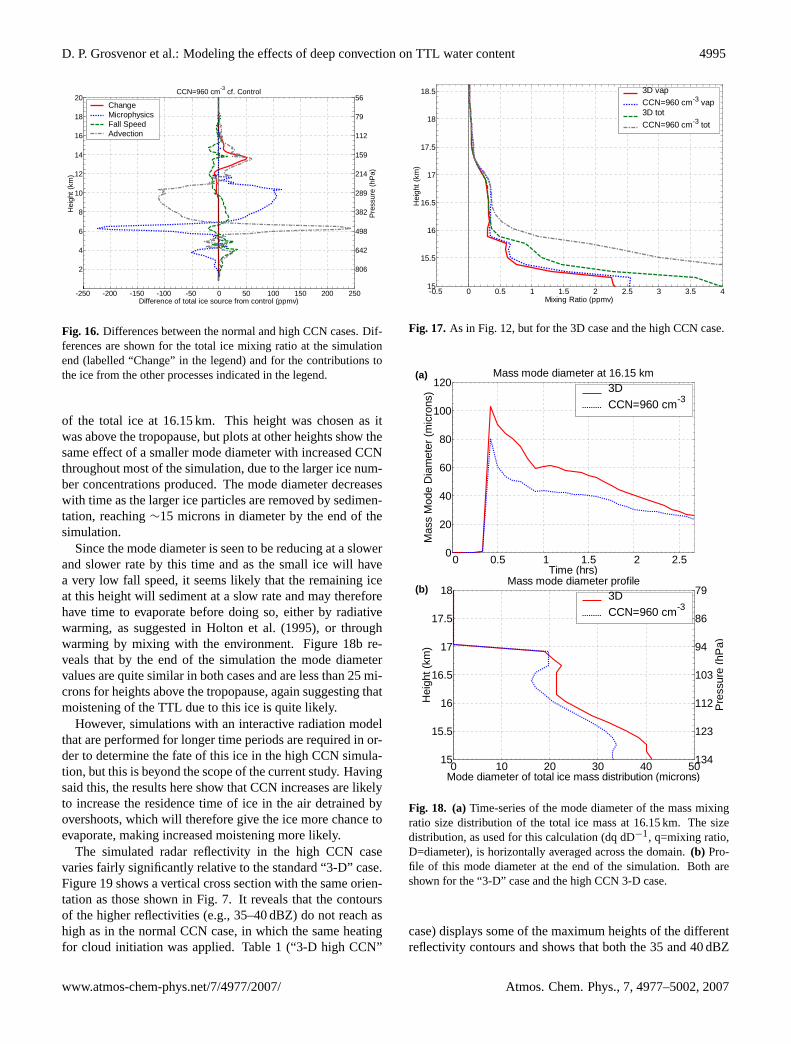
D. P. Grosvenor et al.: Modeling the effects of deep convection on TTL water content 4995
806
642
498
382
289
214
159
112
79
56
Pres
sure
(hP
a)
-250 -200 -150 -100 -50 0 50 100 150 200 250
2
4
6
8
10
12
14
16
18
20
Difference of total ice source from control (ppmv)
Hei
ght (
km)
CCN=960 cm-3 cf. Control
ChangeMicrophysicsFall SpeedAdvection
Fig. 16. Differences between the normal and high CCN cases. Dif-ferences are shown for the total ice mixing ratio at the simulationend (labelled “Change” in the legend) and for the contributions tothe ice from the other processes indicated in the legend.
of the total ice at 16.15 km. This height was chosen as itwas above the tropopause, but plots at other heights show thesame effect of a smaller mode diameter with increased CCNthroughout most of the simulation, due to the larger ice num-ber concentrations produced. The mode diameter decreaseswith time as the larger ice particles are removed by sedimen-tation, reaching∼15 microns in diameter by the end of thesimulation.
Since the mode diameter is seen to be reducing at a slowerand slower rate by this time and as the small ice will havea very low fall speed, it seems likely that the remaining iceat this height will sediment at a slow rate and may thereforehave time to evaporate before doing so, either by radiativewarming, as suggested in Holton et al. (1995), or throughwarming by mixing with the environment. Figure18b re-veals that by the end of the simulation the mode diametervalues are quite similar in both cases and are less than 25 mi-crons for heights above the tropopause, again suggesting thatmoistening of the TTL due to this ice is quite likely.
However, simulations with an interactive radiation modelthat are performed for longer time periods are required in or-der to determine the fate of this ice in the high CCN simula-tion, but this is beyond the scope of the current study. Havingsaid this, the results here show that CCN increases are likelyto increase the residence time of ice in the air detrained byovershoots, which will therefore give the ice more chance toevaporate, making increased moistening more likely.
The simulated radar reflectivity in the high CCN casevaries fairly significantly relative to the standard “3-D” case.Figure19shows a vertical cross section with the same orien-tation as those shown in Fig.7. It reveals that the contoursof the higher reflectivities (e.g., 35–40 dBZ) do not reach ashigh as in the normal CCN case, in which the same heatingfor cloud initiation was applied. Table 1 (“3-D high CCN”
-0.5 0 0.5 1 1.5 2 2.5 3 3.5 415
15.5
16
16.5
17
17.5
18
18.5
Mixing Ratio (ppmv)
Hei
ght (
km)
3D vapCCN=960 cm-3 vap3D totCCN=960 cm-3 tot
Fig. 17. As in Fig.12, but for the 3D case and the high CCN case.
0 0.5 1 1.5 2 2.50
20
40
60
80
100
120
Time (hrs)
Mas
s M
ode
Dia
met
er (m
icro
ns)
Mass mode diameter at 16.15 km3DCCN=960 cm-3
134
123
112
103
94
86
79
Pre
ssur
e (h
Pa)
0 10 20 30 40 5015
15.5
16
16.5
17
17.5
18
Mode diameter of total ice mass distribution (microns)
Hei
ght (
km)
Mass mode diameter profile3DCCN=960 cm-3
(a)
(b)
Fig. 18. (a)Time-series of the mode diameter of the mass mixingratio size distribution of the total ice mass at 16.15 km. The sizedistribution, as used for this calculation (dq dD−1, q=mixing ratio,D=diameter), is horizontally averaged across the domain.(b) Pro-file of this mode diameter at the end of the simulation. Both areshown for the “3-D” case and the high CCN 3-D case.
case) displays some of the maximum heights of the differentreflectivity contours and shows that both the 35 and 40 dBZ
www.atmos-chem-phys.net/7/4977/2007/ Atmos. Chem. Phys., 7, 4977–5002, 2007
4996 D. P. Grosvenor et al.: Modeling the effects of deep convection on TTL water content
-60 -40 -20 0 20 40 60
2
4
6
8
10
12
14
16
18
20
22
Horizontal Distance (km)
Hei
ght (
km)
Radar reflectivity (dBZ)Time = 00:30
10
15
20
25
30
35
40
45
50
55
60
65
703D high CCN
-60 -40 -20 0 20 40 60
2
4
6
8
10
12
14
16
18
20
22
Horizontal Distance (km)
Hei
ght (
km)
Radar reflectivity (dBZ)Time = 00:30
10
15
20
25
30
35
40
45
50
55
60
65
703D high CCN
Fig. 19. Cross section of the simulated radar reflectivity of the 3-Dhign CCN case taken though the slice inidicated in Fig.6.
contours are considerably lower in the high CCN case. Thedifferences are due to the fact that more of the water mass inthe upper regions of the high CCN cloud is in the smaller-sized snow hydrometeor form rather than graupel, since thelack of warm rain produced in the lower regions of the cloudmeans that less graupel can form through raindrop freezing.Hence, the cloud has simulated reflectivities that are consis-tent with more of the observed clouds. When these higherfrequencies are used in the calculation ofdQ, combined withthe higher amounts of moistening seen in the high CCN sim-ulation, significantly higher values are obtained relative tothe normal case (Table 3). For the 16–17 km height range,dQ values of∼0.1–0.3 ppmv are predicted when using thedifferent reflectivity contours and for the 15–16 km range,values of 0.3–1 ppmv are produced.
In both cases, the calculations using the 35 dBZ echo topstatistics gave the smallestdQ values since this contour stillreached fairly high altitudes in the high CCN case. This sug-gests that an adjustment of the droplet number in the bulkmicrophysics scheme still cannot replicate the low reflectivi-ties observed by the radar. In addition, it seems unlikely thatdroplet concentrations in the boundary layer were as high asthose simulated in the high CCN case (960 cm−3) since thebulk of the region is likely to have been moderately unpol-luted. Therefore, whilst suggesting that microphysical tun-ing may help to create clouds that better match the observa-tions, it seems unlikely that the real clouds observed wouldhave been affected by exactly the same microphysical path-ways that led to reduced graupel formation in the high CCNsimulation. Further investigation is required to look into thereasons for the discrepancies.
3.5 Supporting observations from during HIBISCUS
The idea of the injection of air into the stratosphere of thisregion by convection is supported by observations presentedin Nielsen et al. (2007, hereafter referred to as N07) of solidparticles in the lower stratosphere that were made a few daysearlier and at the same location. Back trajectories showed
0 5 10 15x 10
4
14
15
16
17
18
19
20
21
22
Max ice number concentration (kg-1)
Hei
ght (
km)
Max ice NC
3D
Fig. 20. Profile of the maximum ice number concentration at theend of the simulation for the “3-D” case.
the likelihood that these emanated from a particularly in-tense storm that reached 20±1 km in altitude and was located∼200 km east of the observation location∼5.5 h earlier. Itwas speculated that they may have been composed of ice orpartly of NAT (nitric acid tri-hydrate), which would suggestthat moistening had also occurred in order to prevent theirevaporation.
Similar to the observations in N07, in the 3-D simulationof the most vigorous cloud (case “3-D”), an area with highice number concentrations in a small region below 18 km,above the main region of ice left over from the cloud, ispresent 3:35 h after the overshoot reached the TTL regionas shown by the profile of maximum ice number concen-tration in Fig. 20. This result suggests that ice particlescan survive at high altitudes for several hours after injec-tion by deep convection, in concordance with the hypothe-sis presented in N07. It was suggested there that large wa-ter vapour concentrations of around 160 ppmv were requiredto have been transported by the overshooting cloud, in or-der to allow the ice to survive for such a long period. Hori-zontal cross sections of the simulated vapour mixing ratio at17.9 km (Fig.21) show that moderately high vapour amountsof up to almost 9 ppmv were transported along with the iceparticles in the simulation. This suggests that ice particlescan survive in the presence of much lower vapour mixing ra-tios than the 160 ppmv suggested in N07.
The same plot shows that this region was subsaturated withrespect to ice at this time by around 10% or more and hencesublimation of the ice would be expected to be occurring.However, the timeseries of the maximum supersaturation atthis height (Fig.22) shows that such subsaturation only oc-curred at this height during the last 50 min of the simulation.This early supersaturation was due to the cold temperaturesproduced by the cloud as it overshot its level of neutral buoy-ancy, with the air gradually warming and becoming subsatu-rated as it mixed with its surroundings.
Atmos. Chem. Phys., 7, 4977–5002, 2007 www.atmos-chem-phys.net/7/4977/2007/
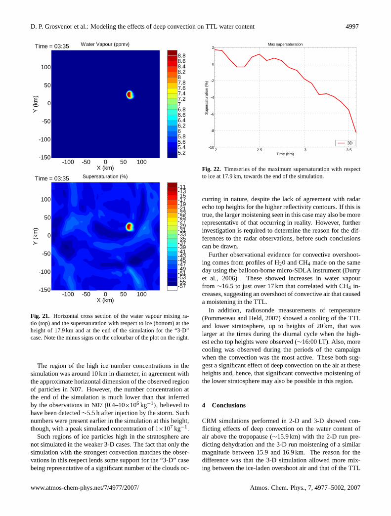
D. P. Grosvenor et al.: Modeling the effects of deep convection on TTL water content 4997
-100 -50 0 50 100-150
-100
-50
0
50
100
X (km)
Y (k
m)
Supersaturation (%)Time = 03:35
-57-55-53-51-49-47-45-43-41-39-37-35-33-31-29-27-25-23-21-19-17-15-13-11
-100 -50 0 50 100-150
-100
-50
0
50
100
X (km)
Y (k
m)
Water Vapour (ppmv)Time = 03:35
5.25.45.65.866.26.46.66.877.27.47.67.888.28.48.68.8
-100 -50 0 50 100-150
-100
-50
0
50
100
X (km)
Y (k
m)
Supersaturation (%)Time = 03:35
-57-55-53-51-49-47-45-43-41-39-37-35-33-31-29-27-25-23-21-19-17-15-13-11
-100 -50 0 50 100-150
-100
-50
0
50
100
X (km)
Y (k
m)
Water Vapour (ppmv)Time = 03:35
5.25.45.65.866.26.46.66.877.27.47.67.888.28.48.68.8
Fig. 21. Horizontal cross section of the water vapour mixing ra-tio (top) and the supersaturation with respect to ice (bottom) at theheight of 17.9 km and at the end of the simulation for the “3-D”case. Note the minus signs on the colourbar of the plot on the right.
The region of the high ice number concentrations in thesimulation was around 10 km in diameter, in agreement withthe approximate horizontal dimension of the observed regionof particles in N07. However, the number concentration atthe end of the simulation is much lower than that inferredby the observations in N07 (0.4–10×106 kg−1), believed tohave been detected∼5.5 h after injection by the storm. Suchnumbers were present earlier in the simulation at this height,though, with a peak simulated concentration of 1×10⁷ kg−1.
Such regions of ice particles high in the stratosphere arenot simulated in the weaker 3-D cases. The fact that only thesimulation with the strongest convection matches the obser-vations in this respect lends some support for the “3-D” casebeing representative of a significant number of the clouds oc-
2 2.5 3 3.5-10
-8
-6
-4
-2
0
2
Time (hrs)
Supe
rsat
urat
ion
(%)
Max supersaturation
3D
Fig. 22. Timeseries of the maximum supersaturation with respectto ice at 17.9 km, towards the end of the simulation.
curring in nature, despite the lack of agreement with radarecho top heights for the higher reflectivity contours. If this istrue, the larger moistening seen in this case may also be morerepresentative of that occurring in reality. However, furtherinvestigation is required to determine the reason for the dif-ferences to the radar observations, before such conclusionscan be drawn.
Further observational evidence for convective overshoot-ing comes from profiles of H20 and CH4 made on the sameday using the balloon-borne micro-SDLA instrument (Durryet al., 2006). These showed increases in water vapourfrom ∼16.5 to just over 17 km that correlated with CH4 in-creases, suggesting an overshoot of convective air that causeda moistening in the TTL.
In addition, radiosonde measurements of temperature(Pommereau and Held, 2007) showed a cooling of the TTLand lower stratosphere, up to heights of 20 km, that waslarger at the times during the diurnal cycle when the high-est echo top heights were observed (∼16:00 LT). Also, morecooling was observed during the periods of the campaignwhen the convection was the most active. These both sug-gest a significant effect of deep convection on the air at theseheights and, hence, that significant convective moistening ofthe lower stratosphere may also be possible in this region.
4 Conclusions
CRM simulations performed in 2-D and 3-D showed con-flicting effects of deep convection on the water content ofair above the tropopause (∼15.9 km) with the 2-D run pre-dicting dehydration and the 3-D run moistening of a similarmagnitude between 15.9 and 16.9 km. The reason for thedifference was that the 3-D simulation allowed more mix-ing between the ice-laden overshoot air and that of the TTL
www.atmos-chem-phys.net/7/4977/2007/ Atmos. Chem. Phys., 7, 4977–5002, 2007
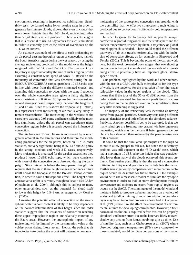
4998 D. P. Grosvenor et al.: Modeling the effects of deep convection on TTL water content
environment, resulting in increased ice sublimation. Sensi-tivity tests, performed using lower heating rates in order togenerate less intense clouds, showed that even in clouds thatreach lower heights than the 2-D cloud, moistening ratherthan dehydration was still produced. These results suggestthat it is essential to use 3-D dynamics for such simulationsin order to correctly predict the effect of overshoots on theTTL water content.
An estimate was made of the effect of such moistening onan air parcel passing through a region of convection, namelythe South America region during the wet season, by using theaverage moistening predicted by the model over the heightranges of both 15–16 km and 16–17 km. The time spent by atrajectory is approximated by the size of such a region, whilstassuming a constant wind speed of 5 m s−1. Based on thefrequency of convection that was observed during the HI-BISCUS/TROCCIBRAS campaign to have 10 dBZ echo topsin line with those from the different simulated clouds, andassuming this convection to occur with the same frequencyover the whole convective area, gives a fairly significantmean moistening of 0.26 and 0.13 ppmv for the strongest andsecond strongest cases, respectively, between the heights of16 and 17 km. Since this is above the tropopause (15.9 km),this represents direct moistening of air that is very likely toremain stratospheric. The moistening in the weakest of thecases here was only 0.05 ppmv and hence is likely to be muchless significant, unless the air parcel can experience manyconvective regions before it ascends beyond the influence ofconvection.
The air between 15 and 16 km is moistened by a muchgreater amount in the simulations and therefore the moist-ening predictions for the air parcel, based on 10 dBZ radarstatistics, are very significant, being 0.85, 1.17 and 2.8 ppmvin the strong, medium and weak 3-D cases, respectively.More moistening is predicted for the weaker cases since theyproduced lower 10 dBZ echo tops, which were consistentwith more of the convective cells observed during the cam-paign. Since this air is below the tropopause, though, thisrequires that the air in these height ranges experiences futureuplift across the tropopause via the Brewer Dobson circula-tion, in order to have a stratospheric effect. The height of netzero radiative uplift is currently thought to lie at∼15±0.5 km(Gettelman et al., 2004), although this is subject to manyother uncertainties, such as the potential for cloud itselfto lower this height by 0.5–1 km, as suggested by Corti etal. (2005).
Assessing the potential effect of convection on the strato-spheric water vapour content is likely to be very dependenton the correct determination of this height since the radarstatistics suggest that the instances of convection reachingthese upper tropospheric regions are relatively common inthe Bauru area. However, the stratospheric impact of anymoistening will be limited by the ice saturation value at thecoldest point during future ascent. Hence, the path that airtrajectories take during the ascent will determine how much
moistening of the stratosphere convection can provide, withthe possibility that no effective stratospheric moistening isproduced due to convection if sufficiently cold temperaturesare reached.
In order to gauge the frequency that air parcels sampleconvective regions during ascent into the stratosphere and thecoldest temperatures reached by them, a trajectory or globalmodel approach is needed. These could model the differentpathways of air as it travels horizontally, but with the inclu-sion of convective effects, as for example in Sherwood andDessler (2001). This is beyond the scope of the current workhere, but the work presented does suggest that overshootingconvection is frequent enough and has enough of a moist-ening effect to potentially have an important global strato-spheric effect.
One problem, highlighted by this work and other authors,with the use of a CRM with bulk microphysics for this typeof work, is the tendency for the prediction of too high radarreflectivity values in the upper regions of the cloud. Thismeans that if the tops of the 35 or 40 dBZ echoes from theradar statistics are used for frequency predictions by com-paring them to the heights achieved in the simulations, thenvery little moistening is suggested.
The majority of the reflectivity was identified as havingcome from graupel particles. Sensitivity tests using differentgraupel densities reveal little effect on the simulated radar re-flectivity. Another possibility, yet to be explored, is that toomany raindrops are freezing into graupel via heterogeneousnucleation, which may be the case if heterogeneous ice nu-clei are less abundant than assumed by the parameterisationsof this process.
It could be that the simulated updraughts are too high soas not to allow graupel to fall out, but since the reflectivityproblem was still apparent in the “3-D-weak” case, whichhad a maximum 10 dBZ echo top height that was consider-ably lower than many of the clouds observed, this seems un-likely. One further possibility is that the use of a convectiveinitiation technique analogous to a warm bubble is the cause.Further investigation by comparison with more natural tech-niques would be desirable for future studies. One examplewould be to use a mesoscale model to simulate the synopticenvironment in order to look at storm development throughconvergence and moisture transport from tropical regions, asoccurs via the SACZ. The spinning up of the model wind andmoisture fields to produce turbulent motions on a variety ofscales and to allow mixing of moisture within the boundarylayer may be an important process as described in Carpenteret al. (1998) since it might affect the entrainment of environ-mental air into the developing warm bubble. However, a finerhorizontal resolution is required before this can be properlysimulated and hence errors due to the latter are likely to over-shadow any arising from issues involving spin up time. Useof satellite data, such as in Chaboureau et al. (2007) whereobserved brightness temperatures (BTs) were compared tothose simulated, would facilitate comparisons of the smaller
Atmos. Chem. Phys., 7, 4977–5002, 2007 www.atmos-chem-phys.net/7/4977/2007/
D. P. Grosvenor et al.: Modeling the effects of deep convection on TTL water content 4999
ice crystals. This would allow further probing of the discrep-ancies between the model and reality and might shed somelight on the reasons for the differences in radar reflectivitiesas well as discerning whether these differences affect the pro-cesses at cloud top.
The results presented here suggest that microphysical con-siderations are likely to be very important to the way a cloudaffects the TTL water content. The number concentrationof ice in the simulated overshoot, as it reached the TTL re-gion, was dominated by crystals that were transported frombelow the TTL, which formed mainly from the homogeneousfreezing of liquid water droplets at –38◦C. For this reason, in3-D sensitivity tests, CCN increases were seen to enhanceice concentrations in the TTL region and led to increased iceevaporation above the tropopause, with∼13% more vapourincrease observed between 15 and 17 km, relative to the in-crease in the normal case.
Very large increases in the amount of extra total water of34 and 132% were found with increasing CCN for the 15–16 and 16–17 km height ranges, respectively, indicating thepresence of substantial additional ice. Whether this ice willsediment slowly enough to evaporate and cause a permanentmoistening of the lower TTL is, however, uncertain, and willrequire further work over longer time scale simulations toascertain. Having said this, the increases in vapour abovethe tropopause and the small sizes of the remaining ice sug-gest that aerosol increases near cloud base could potentiallyhave an impact on the stratospheric vapour content, in agree-ment with Sherwood (2002). It may be possible that suchvariations could account for the observed increasing trendin stratospheric water vapour but further assessment of theglobal scale impact of deep convective water vapour effectsare needed before the likelihood of this can be judged. An ad-ditional source of variability from aerosol effects may comethrough their potential impact on cloud dynamics. Somestudies suggest that CCN numbers may affect the vigour oftropical, deep convection (e.g. Connolly et al., 2007). If thisis the case, then the kind of variability in the moistening ob-served between the three different strengths of cases simu-lated here might be found in nature as a result of aerosol in-teractions, which would allow more potential stratosphericwater vapour trend from aerosol effects.
These results are, of course, subject to the microphysi-cal parameterisations employed by the model. Although abulk microphysics scheme is used here, the prediction of in-creased droplet numbers at cloud base leading to increasedice numbers in the upper cloud is in agreement with ex-plicit microphysics studies (e.g. Khain and Pokrovsky, 2004;Phillips et al., 2002). Improvements in the microphysicalrepresentation of aerosols are desirable for future studies,though. Sensitivity to the parameterisation of the fall speedsof ice should also be examined, given the lack of observa-tional evidence and the importance of this to the residencetime of ice in the TTL.
The current model does not include the effect of the ho-mogeneous freezing of aerosol, only nucleation of heteroge-neous ice nuclei. Jensen and Ackerman (2006) showed thatthe former process could be important in determining the icenumber concentration in the upper regions of deep convec-tion, in contrast to this work, where ice advected from be-low dominated the ice number in the TTL region. This couldhave implications for the effect of convection on the TTL wa-ter content since the homogeneous aerosol freezing in Jensenand Ackerman (2006) was shown to produce numerous smallice particles, which would be unlikely to sediment efficientlyfrom the region and may prevent any dehydration effect or in-crease moistening. It might also reduce the sensitivity of theconvective effect on TTL water content to aerosol loading inthe boundary layer, since even clouds in a clean environmentmay still contain numerous haze droplets and hence producerelatively large ice number concentrations via homogeneousfreezing of aerosol.
However, the onset of homogeneous freezing of aerosolis likely to require that most of the ice particles formed lowin the cloud are removed by the time the cloud reaches highaltitudes since the process requires high supersaturations of∼60% and any remaining ice crystals will tend to act as asink for vapour. It is unclear whether this would occur inall cases. In addition, any IN left over from nucleation fur-ther below, or entrained during ascent, may also prevent highsupersaturations and therefore homogeneous aerosol freez-ing. Given the great uncertainty in IN concentrations and therepresentation of nucleation mechanisms, the effect of thisis likely to be difficult to gauge using current microphysicalmodels.
The simulated reflectivity in the high CCN case wasfound to be more realistic due to reduced graupel produc-tion through raindrop freezing, since less warm rain was pro-duced by the smaller droplets. This suggests a possible mi-crophysical cause for the discrepancies, but since the higherCCN number tested (960 cm−3) is likely to have been abovethat which occurred in the fairly unpolluted test region at thetime of the HIBISCUS campaign, the exact microphysicalmechanisms simulated in this sensitivity test seem unlikelyto have occurred in reality.
It is unknown whether the microphysical differences sug-gested by the enhanced simulated reflectivities high in thecloud will have an effect on the amount of TTL moisteningpredicted by the model. Given that droplet number increaseswere found to have had an effect through ice fall speed con-siderations, this is a possibility. However, since graupel par-ticles are relatively heavy, they are likely to quickly fall fromthe upper regions of the cloud and have little moistening ef-fect. Therefore, the predicted vapour increases may be anunderestimate compared to a situation where smaller ice par-ticles were formed, although it is possible be that more com-plicated microphysical feedbacks, due to the extra graupel,have a compensating effect. The fact that the convection inthe studied season was observed to have been less intense
www.atmos-chem-phys.net/7/4977/2007/ Atmos. Chem. Phys., 7, 4977–5002, 2007
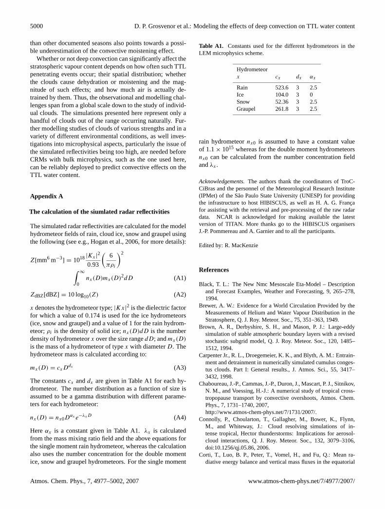
5000 D. P. Grosvenor et al.: Modeling the effects of deep convection on TTL water content
than other documented seasons also points towards a possi-ble underestimation of the convective moistening effect.
Whether or not deep convection can significantly affect thestratospheric vapour content depends on how often such TTLpenetrating events occur; their spatial distribution; whetherthe clouds cause dehydration or moistening and the mag-nitude of such effects; and how much air is actually de-trained by them. Thus, the observational and modelling chal-lenges span from a global scale down to the study of individ-ual clouds. The simulations presented here represent only ahandful of clouds out of the range occurring naturally. Fur-ther modelling studies of clouds of various strengths and in avariety of different environmental conditions, as well inves-tigations into microphysical aspects, particularly the issue ofthe simulated reflectivities being too high, are needed beforeCRMs with bulk microphysics, such as the one used here,can be reliably deployed to predict convective effects on theTTL water content.
Appendix A
The calculation of the siumlated radar reflectivities
The simulated radar reflectivities are calculated for the modelhydrometeor fields of rain, cloud ice, snow and graupel usingthe following (see e.g., Hogan et al., 2006, for more details):
Z[mm6 m−3] = 1018|Kx |
2
0.93
(6
πρi
)2
∫∞
0nx(D)mx(D)2dD (A1)
ZdBZ[dBZ] = 10 log10(Z) (A2)
x denotes the hydrometeor type;|Kx|2 is the dielectric factor
for which a value of 0.174 is used for the ice hydrometeors(ice, snow and graupel) and a value of 1 for the rain hydrom-eteor;ρi is the density of solid ice;nx(D)dD is the numberdensity of hydrometeorx over the size rangedD; andmx(D)
is the mass of a hydrometeor of typex with diameterD. Thehydrometeor mass is calculated according to:
mx(D) = cxDdx (A3)
The constantscx anddx are given in TableA1 for each hy-drometeor. The number distribution as a function of size isassumed to be a gamma distribution with different parame-ters for each hydrometeor:
nx(D) = nx0Dαx e−λxD (A4)
Hereαx is a constant given in TableA1. λx is calculatedfrom the mass mixing ratio field and the above equations forthe single moment rain hydrometeor, whereas the calculationalso uses the number concentration for the double momentice, snow and graupel hydrometeors. For the single moment
Table A1. Constants used for the different hydrometeors in theLEM microphysics scheme.
Hydrometeorx cx dx αx
Rain 523.6 3 2.5Ice 104.0 3 0Snow 52.36 3 2.5Graupel 261.8 3 2.5
rain hydrometeornx0 is assumed to have a constant valueof 1.1 × 10¹⁵ whereas for the double moment hydrometeorsnx0 can be calculated from the number concentration fieldandλx .
Acknowledgements.The authors thank the coordinators of TroC-CiBras and the personnel of the Meteorological Research Institute(IPMet) of the Sao Paulo State University (UNESP) for providingthe infrastructure to host HIBISCUS, as well as H. A. G. Francafor assisting with the retrieval and pre-processing of the raw radardata. NCAR is acknowledged for making available the latestversion of TITAN. More thanks go to the HIBISCUS organisersJ.-P. Pommereau and A. Garnier and to all the participants.
Edited by: R. MacKenzie
References
Black, T. L.: The New Nmc Mesoscale Eta-Model – Descriptionand Forecast Examples, Weather and Forecasting, 9, 265–278,1994.
Brewer, A. W.: Evidence for a World Circulation Provided by theMeasurements of Helium and Water Vapour Distribution in theStratosphere, Q. J. Roy. Meteor. Soc., 75, 351–363, 1949.
Brown, A. R., Derbyshire, S. H., and Mason, P. J.: Large-eddysimulation of stable atmospheric boundary layers with a revisedstochastic subgrid model, Q. J. Roy. Meteor. Soc., 120, 1485–1512, 1994.
Carpenter Jr., R. L., Droegemeier, K. K., and Blyth, A. M.: Entrain-ment and detrainment in numerically simulated cumulus conges-tus clouds. Part I: General results., J. Atmos. Sci., 55, 3417–3432, 1998.
Chaboureau, J.-P., Cammas, J.-P., Duron, J., Mascart, P. J., Sitnikov,N. M., and Voessing, H.-J.: A numerical study of tropical cross-tropopause transport by convective overshoots, Atmos. Chem.Phys., 7, 1731–1740, 2007,http://www.atmos-chem-phys.net/7/1731/2007/.
Connolly, P., Choularton, T., Gallagher, M., Bower, K., Flynn,M., and Whiteway, J.: Cloud resolving simulations of in-tense tropical, Hector thunderstorms: Implications for aerosol-cloud interactions, Q. J. Roy. Meteor. Soc., 132, 3079–3106,doi:10.1256/qj.05.86, 2006.
Corti, T., Luo, B. P., Peter, T., Vomel, H., and Fu, Q.: Mean ra-diative energy balance and vertical mass fluxes in the equatorial
Atmos. Chem. Phys., 7, 4977–5002, 2007 www.atmos-chem-phys.net/7/4977/2007/
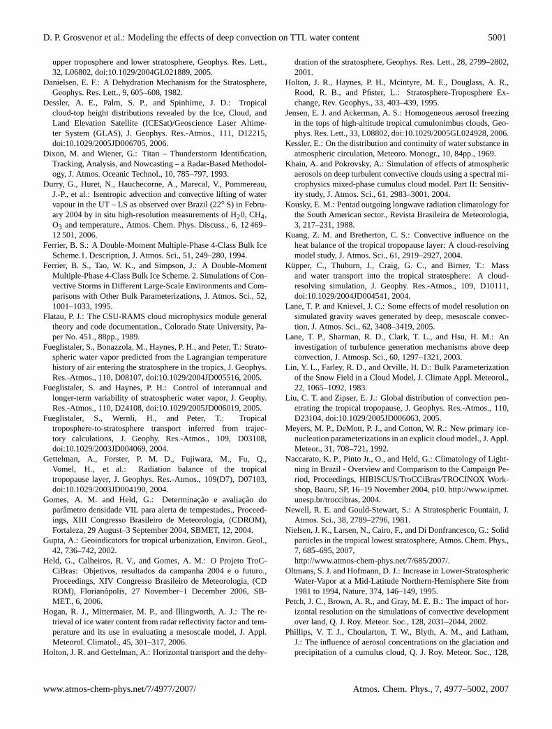
D. P. Grosvenor et al.: Modeling the effects of deep convection on TTL water content 5001
upper troposphere and lower stratosphere, Geophys. Res. Lett.,32, L06802, doi:10.1029/2004GL021889, 2005.
Danielsen, E. F.: A Dehydration Mechanism for the Stratosphere,Geophys. Res. Lett., 9, 605–608, 1982.
Dessler, A. E., Palm, S. P., and Spinhirne, J. D.: Tropicalcloud-top height distributions revealed by the Ice, Cloud, andLand Elevation Satellite (ICESat)/Geoscience Laser Altime-ter System (GLAS), J. Geophys. Res.-Atmos., 111, D12215,doi:10.1029/2005JD006705, 2006.
Dixon, M. and Wiener, G.: Titan – Thunderstorm Identification,Tracking, Analysis, and Nowcasting – a Radar-Based Methodol-ogy, J. Atmos. Oceanic Technol., 10, 785–797, 1993.
Durry, G., Huret, N., Hauchecorne, A., Marecal, V., Pommereau,J.-P., et al.: Isentropic advection and convective lifting of watervapour in the UT – LS as observed over Brazil (22◦ S) in Febru-ary 2004 by in situ high-resolution measurements of H20, CH4,O3 and temperature., Atmos. Chem. Phys. Discuss., 6, 12 469–12 501, 2006.
Ferrier, B. S.: A Double-Moment Multiple-Phase 4-Class Bulk IceScheme.1. Description, J. Atmos. Sci., 51, 249–280, 1994.
Ferrier, B. S., Tao, W. K., and Simpson, J.: A Double-MomentMultiple-Phase 4-Class Bulk Ice Scheme. 2. Simulations of Con-vective Storms in Different Large-Scale Environments and Com-parisons with Other Bulk Parameterizations, J. Atmos. Sci., 52,1001–1033, 1995.
Flatau, P. J.: The CSU-RAMS cloud microphysics module generaltheory and code documentation., Colorado State University, Pa-per No. 451., 88pp., 1989.
Fueglistaler, S., Bonazzola, M., Haynes, P. H., and Peter, T.: Strato-spheric water vapor predicted from the Lagrangian temperaturehistory of air entering the stratosphere in the tropics, J. Geophys.Res.-Atmos., 110, D08107, doi:10.1029/2004JD005516, 2005.
Fueglistaler, S. and Haynes, P. H.: Control of interannual andlonger-term variability of stratospheric water vapor, J. Geophy.Res.-Atmos., 110, D24108, doi:10.1029/2005JD006019, 2005.
Fueglistaler, S., Wernli, H., and Peter, T.: Tropicaltroposphere-to-stratosphere transport inferred from trajec-tory calculations, J. Geophy. Res.-Atmos., 109, D03108,doi:10.1029/2003JD004069, 2004.
Gettelman, A., Forster, P. M. D., Fujiwara, M., Fu, Q.,Vomel, H., et al.: Radiation balance of the tropicaltropopause layer, J. Geophys. Res.-Atmos., 109(D7), D07103,doi:10.1029/2003JD004190, 2004.
Gomes, A. M. and Held, G.: Determinacao e avaliacao doparametro densidade VIL para alerta de tempestades., Proceed-ings, XIII Congresso Brasileiro de Meteorologia, (CDROM),Fortaleza, 29 August–3 September 2004, SBMET, 12, 2004.
Gupta, A.: Geoindicators for tropical urbanization, Environ. Geol.,42, 736–742, 2002.
Held, G., Calheiros, R. V., and Gomes, A. M.: O Projeto TroC-CiBras: Objetivos, resultados da campanha 2004 e o futuro.,Proceedings, XIV Congresso Brasileiro de Meteorologia, (CDROM), Florianopolis, 27 November–1 December 2006, SB-MET., 6, 2006.
Hogan, R. J., Mittermaier, M. P., and Illingworth, A. J.: The re-trieval of ice water content from radar reflectivity factor and tem-perature and its use in evaluating a mesoscale model, J. Appl.Meteorol. Climatol., 45, 301–317, 2006.
Holton, J. R. and Gettelman, A.: Horizontal transport and the dehy-
dration of the stratosphere, Geophys. Res. Lett., 28, 2799–2802,2001.
Holton, J. R., Haynes, P. H., Mcintyre, M. E., Douglass, A. R.,Rood, R. B., and Pfister, L.: Stratosphere-Troposphere Ex-change, Rev. Geophys., 33, 403–439, 1995.
Jensen, E. J. and Ackerman, A. S.: Homogeneous aerosol freezingin the tops of high-altitude tropical cumulonimbus clouds, Geo-phys. Res. Lett., 33, L08802, doi:10.1029/2005GL024928, 2006.
Kessler, E.: On the distribution and continuity of water substance inatmospheric circulation, Meteoro. Monogr., 10, 84pp., 1969.
Khain, A. and Pokrovsky, A.: Simulation of effects of atmosphericaerosols on deep turbulent convective clouds using a spectral mi-crophysics mixed-phase cumulus cloud model. Part II: Sensitiv-ity study, J. Atmos. Sci., 61, 2983–3001, 2004.
Kousky, E. M.: Pentad outgoing longwave radiation climatology forthe South American sector., Revista Brasileira de Meteorologia,3, 217–231, 1988.
Kuang, Z. M. and Bretherton, C. S.: Convective influence on theheat balance of the tropical tropopause layer: A cloud-resolvingmodel study, J. Atmos. Sci., 61, 2919–2927, 2004.
Kupper, C., Thuburn, J., Craig, G. C., and Birner, T.: Massand water transport into the tropical stratosphere: A cloud-resolving simulation, J. Geophy. Res.-Atmos., 109, D10111,doi:10.1029/2004JD004541, 2004.
Lane, T. P. and Knievel, J. C.: Some effects of model resolution onsimulated gravity waves generated by deep, mesoscale convec-tion, J. Atmos. Sci., 62, 3408–3419, 2005.
Lane, T. P., Sharman, R. D., Clark, T. L., and Hsu, H. M.: Aninvestigation of turbulence generation mechanisms above deepconvection, J. Atmosp. Sci., 60, 1297–1321, 2003.
Lin, Y. L., Farley, R. D., and Orville, H. D.: Bulk Parameterizationof the Snow Field in a Cloud Model, J. Climate Appl. Meteorol.,22, 1065–1092, 1983.
Liu, C. T. and Zipser, E. J.: Global distribution of convection pen-etrating the tropical tropopause, J. Geophys. Res.-Atmos., 110,D23104, doi:10.1029/2005JD006063, 2005.
Meyers, M. P., DeMott, P. J., and Cotton, W. R.: New primary ice-nucleation parameterizations in an explicit cloud model., J. Appl.Meteor., 31, 708–721, 1992.
Naccarato, K. P., Pinto Jr., O., and Held, G.: Climatology of Light-ning in Brazil - Overview and Comparison to the Campaign Pe-riod, Proceedings, HIBISCUS/TroCCiBras/TROCINOX Work-shop, Bauru, SP, 16–19 November 2004, p10.http://www.ipmet.unesp.br/troccibras, 2004.
Newell, R. E. and Gould-Stewart, S.: A Stratospheric Fountain, J.Atmos. Sci., 38, 2789–2796, 1981.
Nielsen, J. K., Larsen, N., Cairo, F., and Di Donfrancesco, G.: Solidparticles in the tropical lowest stratosphere, Atmos. Chem. Phys.,7, 685–695, 2007,http://www.atmos-chem-phys.net/7/685/2007/.
Oltmans, S. J. and Hofmann, D. J.: Increase in Lower-StratosphericWater-Vapor at a Mid-Latitude Northern-Hemisphere Site from1981 to 1994, Nature, 374, 146–149, 1995.
Petch, J. C., Brown, A. R., and Gray, M. E. B.: The impact of hor-izontal resolution on the simulations of convective developmentover land, Q. J. Roy. Meteor. Soc., 128, 2031–2044, 2002.
Phillips, V. T. J., Choularton, T. W., Blyth, A. M., and Latham,J.: The influence of aerosol concentrations on the glaciation andprecipitation of a cumulus cloud, Q. J. Roy. Meteor. Soc., 128,
www.atmos-chem-phys.net/7/4977/2007/ Atmos. Chem. Phys., 7, 4977–5002, 2007
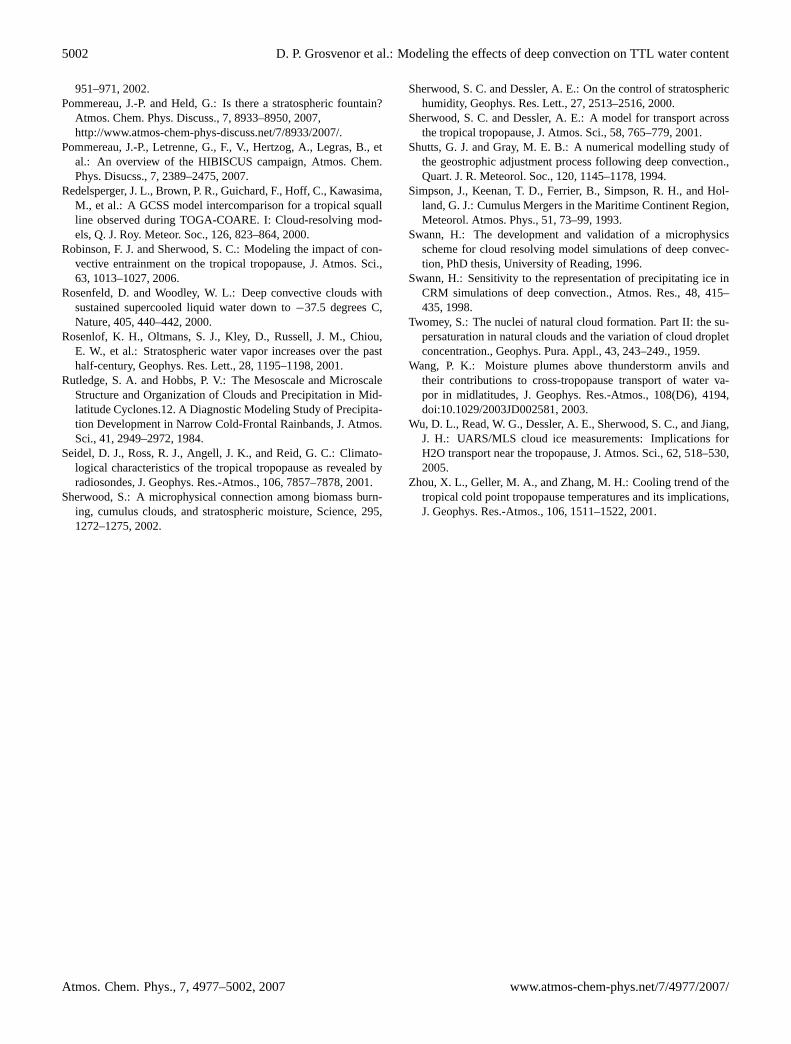
5002 D. P. Grosvenor et al.: Modeling the effects of deep convection on TTL water content
951–971, 2002.Pommereau, J.-P. and Held, G.: Is there a stratospheric fountain?
Atmos. Chem. Phys. Discuss., 7, 8933–8950, 2007,http://www.atmos-chem-phys-discuss.net/7/8933/2007/.
Pommereau, J.-P., Letrenne, G., F., V., Hertzog, A., Legras, B., etal.: An overview of the HIBISCUS campaign, Atmos. Chem.Phys. Disucss., 7, 2389–2475, 2007.
Redelsperger, J. L., Brown, P. R., Guichard, F., Hoff, C., Kawasima,M., et al.: A GCSS model intercomparison for a tropical squallline observed during TOGA-COARE. I: Cloud-resolving mod-els, Q. J. Roy. Meteor. Soc., 126, 823–864, 2000.
Robinson, F. J. and Sherwood, S. C.: Modeling the impact of con-vective entrainment on the tropical tropopause, J. Atmos. Sci.,63, 1013–1027, 2006.
Rosenfeld, D. and Woodley, W. L.: Deep convective clouds withsustained supercooled liquid water down to−37.5 degrees C,Nature, 405, 440–442, 2000.
Rosenlof, K. H., Oltmans, S. J., Kley, D., Russell, J. M., Chiou,E. W., et al.: Stratospheric water vapor increases over the pasthalf-century, Geophys. Res. Lett., 28, 1195–1198, 2001.
Rutledge, S. A. and Hobbs, P. V.: The Mesoscale and MicroscaleStructure and Organization of Clouds and Precipitation in Mid-latitude Cyclones.12. A Diagnostic Modeling Study of Precipita-tion Development in Narrow Cold-Frontal Rainbands, J. Atmos.Sci., 41, 2949–2972, 1984.
Seidel, D. J., Ross, R. J., Angell, J. K., and Reid, G. C.: Climato-logical characteristics of the tropical tropopause as revealed byradiosondes, J. Geophys. Res.-Atmos., 106, 7857–7878, 2001.
Sherwood, S.: A microphysical connection among biomass burn-ing, cumulus clouds, and stratospheric moisture, Science, 295,1272–1275, 2002.
Sherwood, S. C. and Dessler, A. E.: On the control of stratospherichumidity, Geophys. Res. Lett., 27, 2513–2516, 2000.
Sherwood, S. C. and Dessler, A. E.: A model for transport acrossthe tropical tropopause, J. Atmos. Sci., 58, 765–779, 2001.
Shutts, G. J. and Gray, M. E. B.: A numerical modelling study ofthe geostrophic adjustment process following deep convection.,Quart. J. R. Meteorol. Soc., 120, 1145–1178, 1994.
Simpson, J., Keenan, T. D., Ferrier, B., Simpson, R. H., and Hol-land, G. J.: Cumulus Mergers in the Maritime Continent Region,Meteorol. Atmos. Phys., 51, 73–99, 1993.
Swann, H.: The development and validation of a microphysicsscheme for cloud resolving model simulations of deep convec-tion, PhD thesis, University of Reading, 1996.
Swann, H.: Sensitivity to the representation of precipitating ice inCRM simulations of deep convection., Atmos. Res., 48, 415–435, 1998.
Twomey, S.: The nuclei of natural cloud formation. Part II: the su-persaturation in natural clouds and the variation of cloud dropletconcentration., Geophys. Pura. Appl., 43, 243–249., 1959.
Wang, P. K.: Moisture plumes above thunderstorm anvils andtheir contributions to cross-tropopause transport of water va-por in midlatitudes, J. Geophys. Res.-Atmos., 108(D6), 4194,doi:10.1029/2003JD002581, 2003.
Wu, D. L., Read, W. G., Dessler, A. E., Sherwood, S. C., and Jiang,J. H.: UARS/MLS cloud ice measurements: Implications forH2O transport near the tropopause, J. Atmos. Sci., 62, 518–530,2005.
Zhou, X. L., Geller, M. A., and Zhang, M. H.: Cooling trend of thetropical cold point tropopause temperatures and its implications,J. Geophys. Res.-Atmos., 106, 1511–1522, 2001.
Atmos. Chem. Phys., 7, 4977–5002, 2007 www.atmos-chem-phys.net/7/4977/2007/