Embed Size (px)
Citation preview
A Study of Transfer Learning Methods within NaturalLanguage Processing and Reinforcement Learning
Shrishti JeswaniJoseph Gonzalez, Ed.John F. Canny, Ed.
Electrical Engineering and Computer SciencesUniversity of California at Berkeley
Technical Report No. UCB/EECS-2020-98http://www2.eecs.berkeley.edu/Pubs/TechRpts/2020/EECS-2020-98.html
May 29, 2020
Copyright © 2020, by the author(s).All rights reserved.
Permission to make digital or hard copies of all or part of this work forpersonal or classroom use is granted without fee provided that copies arenot made or distributed for profit or commercial advantage and that copiesbear this notice and the full citation on the first page. To copy otherwise, torepublish, to post on servers or to redistribute to lists, requires prior specificpermission.
Acknowledgement
I would like to thank my advisor, Professor Joseph Gonzalez, for providingme with several opportunities and resources during my time at UC Berkeley.I'm very grateful for the Google AdsAI team and my host/mentor, PrincipalScientist Sugato Basu, for giving the opportunity to intern with AdsAI andinspiring my research. I would also like to thank graduate students EricWallace and Charles Packer for their continuous guidance and support in myresearch endeavors. Thank you to my friends, fellow TAs and the RISE labcommunity for the encouragement and memories. Finally, I would like tothank my family for the endless support and guidance throughout my yearsat Berkeley.
Understanding Generalization within Natural Language Processing and Reinforcement Learning
by Shrishti (Sona) Jeswani
Research Project
Submitted to the Department of Electrical Engineering and Computer Sciences, University of California at Berkeley, in partial satisfaction of the requirements for the degree of Master of Science, Plan II.
Approval for the Report and Comprehensive Examination:
Committee:
Professor Joseph GonzalezResearch Advisor
(Date)
* * * * * * *
Professor John CannySecond Reader
(Date)
May 28, 2020
A Study of Transfer Learning Methods within Natural Language Processing andReinforcement Learning
by
Shrishti (Sona) Jeswani
A thesis submitted in partial satisfaction of the
requirements for the degree of
Masters of Science
in
Electrical Engineering and Computer Science
in the
Graduate Division
of the
University of California, Berkeley
Committee in charge:
Professor Joseph Gonzalez, ChairProfessor John Canny
Spring 2020
A Study of Transfer Learning Methods within Natural Language Processing andReinforcement Learning
Copyright 2020by
Shrishti (Sona) Jeswani
1
Abstract
A Study of Transfer Learning Methods within Natural Language Processing andReinforcement Learning
by
Shrishti (Sona) Jeswani1
Masters of Science in Electrical Engineering and Computer Science
University of California, Berkeley
Professor Joseph Gonzalez, Chair
Learning to adapt to new situations in the face of limited experience is the hallmark of humanintelligence. Whether in Natural Language Processing (NLP) or Reinforcement learning(RL), versatility is key for intelligent systems to perform well in the real world. This workwill propose and evaluate solutions to salient transfer learning problems in NLP and RL.
Although today’s pre-trained language models are considerably more robust to out-of-distributiondata than traditional NLP models, they still remain notoriously brittle. We present a test-time training technique for NLP models to adapt to unforeseen distribution shifts at test-time, where no data is available during training time to use for domain adaptation. Ourapproach updates models at test-time using an unsupervised masked language modeling(MLM) objective. We ensure that this auxiliary loss is helpful by training using a gradientalignment technique that pushes the MLM and supervised losses together. We evaluate ourapproach on a variety of di↵erent tasks such as sentiment analysis and semantic similarity.
Although deep RL algorithms enable agents to perform impressive tasks, they often requireseveral trials in order for agents to develop skills within a given environment. Furthermore,agents struggle to adapt to small changes in the environment, requiring additional samples torebuild their knowledge about the world. In contrast, humans and animals are able to rapidlyadapt to changes, while learning quickly from their prior experiences. Our objective is to im-prove generalization performance of state-of-the-art meta-RL approaches, where we considergeneralization to changes in environment dynamics and environment reward structure. Wepropose and evaluate various novel meta-RL architectures, which aim to improve adaptationto new environments by disentangling components of the recurrent policy network.
1Based on paper drafts:
“Handling Unforeseen Distribution Shift Via Test-time Retrieval and Training” written with Eric Wallace
and Joseph E. Gonzalez; “Improving Generalization in RL Through Better Adaptation” written with Charles
Packer, Katelyn Gao and Joseph E. Gonzalez
i
Contents
Contents i
1 Introduction 11.1 Handling Unseen Distribution Shift in NLP . . . . . . . . . . . . . . . . . . 21.2 Improving Generalization in RL Through Better Adaptation . . . . . . . . . 3
2 Transfer Learning Background 52.1 Definition . . . . . . . . . . . . . . . . . . . . . . . . . . . . . . . . . . . . . 52.2 Taxonomy . . . . . . . . . . . . . . . . . . . . . . . . . . . . . . . . . . . . . 5
3 Handling Unseen Distribution Shift in NLP 83.1 Background . . . . . . . . . . . . . . . . . . . . . . . . . . . . . . . . . . . . 83.2 Approach . . . . . . . . . . . . . . . . . . . . . . . . . . . . . . . . . . . . . 103.3 Experiments . . . . . . . . . . . . . . . . . . . . . . . . . . . . . . . . . . . . 133.4 Related Work . . . . . . . . . . . . . . . . . . . . . . . . . . . . . . . . . . . 163.5 Conclusion and Future Work . . . . . . . . . . . . . . . . . . . . . . . . . . . 19
4 Improving Generalization in RL Through Better Adaptation 244.1 Background . . . . . . . . . . . . . . . . . . . . . . . . . . . . . . . . . . . . 244.2 Related Work . . . . . . . . . . . . . . . . . . . . . . . . . . . . . . . . . . . 264.3 Approach . . . . . . . . . . . . . . . . . . . . . . . . . . . . . . . . . . . . . 274.4 Experiments . . . . . . . . . . . . . . . . . . . . . . . . . . . . . . . . . . . . 304.5 Conclusion and Future Work . . . . . . . . . . . . . . . . . . . . . . . . . . . 38
5 Conclusion and Future Work 43
Bibliography 44
ii
Acknowledgments
I would like to thank my advisor, Professor Joseph Gonzalez, for providing me with severalopportunities and resources during my time at UC Berkeley. I’m very grateful for the GoogleAdsAI team and my host/mentor, Principal Scientist Sugato Basu, for giving the opportunityto intern with AdsAI and inspiring my research. I would also like to thank graduate studentsEric Wallace and Charles Packer for their continuous guidance and support in my researchendeavors. Thank you to my friends, fellow TAs and the RISE lab community for theencouragement and memories. Finally, I would like to thank my family for the endlesssupport and guidance throughout my years at Berkeley.
1
Chapter 1
Introduction
The classic supervised machine learning paradigm is based on learning in isolation, whereeach task is solved by using a separate model with a single dataset. Transfer learning is a setof methods used to overcome the isolated learning paradigm by utilizing knowledge acquiredfor one task to solve related ones. By leveraging data from additional domains or tasks,models are able to generalize better and transfer knowledge between tasks. In fact, transferlearning is very reminiscent to how humans approach learning; humans have the inherentability to utilize knowledge/experiences from previous tasks and domains to solve new tasks.
In the last few years, Natural Language Processing (NLP) has witnessed the emergenceof several transfer learning methods and architectures; these techniques have significantlyimproved performance on a wide range of NLP tasks and transformed the landscape of NLPresearch. Similarly, within reinforcement learning (RL), there has been an increased interestin training agents to adapt to di↵erent environments by learning from previous experience.There are several interesting transfer learning applications within NLP and RL; we explorea few of them within this work.
In real-world NLP settings, the examples received at test-time are often drawn froma di↵erent distribution than examples during training. Since many distribution shifts areunforeseen in practice, language models must be robust to out-of-distribution examples attest time without prior knowledge of the distribution shift. In this work, we explore a newsetting where there is no data available during training to anticipate distribution shifts attest-time. We perform a comprehensive study of the robustness of pretrained models andpropose methods that enable models to adapt on-the-fly to new distributions at test-time.
Within the field of RL, enabling agents to quickly learn new tasks by using previousexperience is a well-studied problem. Since it is impractical to train an agent to learneach individual skill in isolation, it is crucial for agents to adapt in order to pick up newskills/tasks faster and handle unseen situations at test time. In this work, we propose andevaluate novel architectures in order to improve generalization to both environment dynamicsand environment reward structure.
CHAPTER 1. INTRODUCTION 2
1.1 Handling Unseen Distribution Shift in NLP
Pretrained language models are foundational for strong performance in a wide variety ofnatural language processing tasks. Pretrained models such as ELMo [42] and BERT [7] aretrained on large, diverse corpora of unlabeled text; as a result, the representations learnedfrom these models have achieved state-of-the-art performance across many downstream taskswith datasets from a diverse set of sources/domains. Although, these pretrained represen-tations have proven to be transferable to a wide range of domains, research still shows thatthere exist generalization gaps between in-domain data and out-of-distribution data [21].
This is a problem because the train and test data are rarely drawn from the same dis-tribution in practice. This distribution mismatch often arises from the natural evolution oftrends, language, and society over time. Accordingly, it is crucial for models to generalizeto out-of-distribution examples. Much of previous research in generalization assumes thatthe distribution shift is known in advance [17, 57], allowing us to apply standard supervisedand unsupervised domain adaptation techniques.
However, in many real-world settings, there is no prior data available to anticipate distri-bution shifts, henceforth unforeseen distribution shift. For example, in fake news detection,models must constantly stay up to date with evolving topics and trends without prior knowl-edge. Furthermore, search engines must recommend results given queries from a very diverseset of evolving users. These real-world settings exemplify the limitations in assuming thedistribution shift is known beforehand.
In our NLP study, we explore a new setting in which the distribution of the examplesreceived during test-time is unknown; in other words, there is no data available duringtraining-time to anticipate distribution shifts. We propose a technique to adapt to unfore-seeable domain/distribution shifts during test-time. Upon receiving an example from anunfamiliar domain during test-time, we believe the language model will greatly benefit fromadditional training (or fine-tuning) on the test example and other similar, relevant examplesusing the unsupervised masked language modeling objective. By taking gradient step(s)using an labeled objective on the test-example, the model is able to get practice reading thedomain and making predictions before actually testing; this is very similar to how humansapproach learning. Using test-time training for out-of-distribution generalization has beenstudied in computer vision [56]; however, these ideas have several unique applications forNLP.
In order for auxiliary tasks to be helpful for the primary task, the tasks must sharesimilarities. One way to measure task similarity is to compute the cosine similarity betweenthe gradients of the tasks [8]. Our test-time training approach only works if the gradientsfrom the masked language modeling objective are roughly aligned with the gradients of thesupervised objective. To this end, we propose a gradient alignment technique to explicitlytrain a model such that the gradients from the masked language modeling objective and thesupervised objective is aligned.
We evaluate our approach on a variety of di↵erent tasks such as sentiment analysis,textual entailment, and semantic similarity.
CHAPTER 1. INTRODUCTION 3
1.2 Improving Generalization in RL Through BetterAdaptation
Deep reinforcement learning (RL) has emerged as an important family of techniques thatlearn to accomplish goals in a variety of complex real-world environments. Deep RL methodshave been shown to learn complex tasks ranging from games [15] to robotic control [29, 51]by simply exploring the environment and receiving rewards.
Although deep reinforcement learning algorithms allow agents to perform impressivetasks, they often require a large number of trials in order for agents to develop skills withina given environment. Furthermore, agents are unable to adapt to small changes in theenvironment and require additional trials/samples in order to rebuild their knowledge aboutthe world. In contrast, humans and animals are able to adapt to changes in the environment,while learning quickly from their prior knowledge about the world. These problems are rootedin how deep RL algorithms are commonly trained and evaluated on a fixed environment;the algorithms are evaluated in terms of their ability to optimize a policy in a complexenvironment, rather than their ability to learn a representation that generalizes to previouslyunseen circumstances.
In principle, meta-reinforcement learning (meta-RL) algorithms enable agents to learnnew skills from small amounts of experience; however, many state-of-the-art model-free meth-ods still struggle to adapt to new environments with di↵erent dynamics using a restrictedamount of new experience.
We are interested in developing methods that enable agents to better adapt to newenvironments that di↵er from those seen during training. In particular, we are interested insettings where environment dynamics (e.g., friction or torque in a Mujoco environment) andenvironment reward structure (e.g., target velocity for a running Mujoco robot) are di↵erentat test time than during training; either from the same distribution of MDPs (interpolation),or from a di↵erent distribution (extrapolation).
Our objective is to improve the generalization performance of state-of-the-art model-free meta-RL approaches, where we are concerned with generalization to both changes inenvironment dynamics and environment reward structure. In line with our objective, wepropose and evaluate various novel meta-RL architectures based on the architecture andtraining algorithm described by previous work (ie. RL2) [10]. Our architectural changes aimto improve adaptation to new environments by disentangling the recurrent and feed forwardcomponents of the recurrent policy network.
CHAPTER 1. INTRODUCTION 4
We begin Chapter 2 by discussing a formal definition of transfer learning, along withdi↵erent settings of transfer learning that arise; this will build a foundation on transferlearning that is necessary for subsequent chapters.
In Chapter 3 of this work, we explore a new NLP setting in which the domain of theexamples received during test-time is unknown; in other words, there is no data availableduring training-time to anticipate distribution shifts. We propose a technique to adapt tounforeseeable domain/distribution shifts during test-time, similar to how humans approachlearning.
In Chapter 4 of this work, we examine meta-learning techniques within RL in orderto develop policies that can adapt to di↵erent tasks and environments at test-time. Wepropose and evaluate various novel meta-RL architectures based on the architecture andtraining algorithm described by [10] (RL2).
5
Chapter 2
Transfer Learning Background
In the classic supervised machine learning setting, if we intend to train a model to solve agiven task and domain, we assume that labelled data is available for the same given task anddomain. This traditional supervised learning paradigm breaks down when labeled data forthe task and domain is scarce. Transfer learning enables us to leverage data from a relatedtask or domain known as a source task or source domain. We seek to apply this knowledgeto the target task or target domain. Knowledge can manifest in several di↵erent forms, butwe primarily link it with the representations learned by neural network models.
2.1 Definition
We provide a formal definition of transfer learning following the notation of previous work [38,48]. We first introduce the concepts of a domain and a task. A domain D consists of afeature space � and a marginal probability distribution P (X) over the feature space, whereX = {x1, ..., xn} 2 �. X is a random variable that represents the sample of data points usedfor training, where each xi is the feature representation of each example.
Given a domain D = {X,P (X)}, a task T consists of a label space Y , a prior distributionP (Y ), and a conditional probability distribution P (Y |X) that is typically learned from thetraining data consisting of pairs xi 2 X and yi 2 Y .
Given a source domain DS, a corresponding source task TS, along with a target domainDT and a target task TT , transfer learning aims to learn the target conditional probabilitydistribution PT (YT |XT ) inDT using the information gained fromDS and TS, whereDS 6= DT
or TS 6= TT .
2.2 Taxonomy
Based on di↵erent situations between the source domains, target domains, source tasks andtarget tasks, transfer learning can be categorized into the following sub-settings [38]:
CHAPTER 2. TRANSFER LEARNING BACKGROUND 6
1. Inductive Transfer Learning: The target task is di↵erent from the source task,regardless of whether the source and target domains are the same or not. This can bewritten as TT 6= TS.
2. Transductive Transfer Learning: The source and target tasks are the same, whilethe source and target domains are di↵erent. This can be written as TS = TT , DS 6= DT .In this scenario, no labeled data in the target domain are available while a lot of labeleddata in the source domain are available.
3. Unsupervised Transfer Learning: The target task is di↵erent from the source task,but related. The primary focus is on solving unsupervised learning tasks in the targetdomain, such as clustering, dimensionality reduction and density estimation. In thiscase, there are no labeled data available in both source and target domains duringtraining.
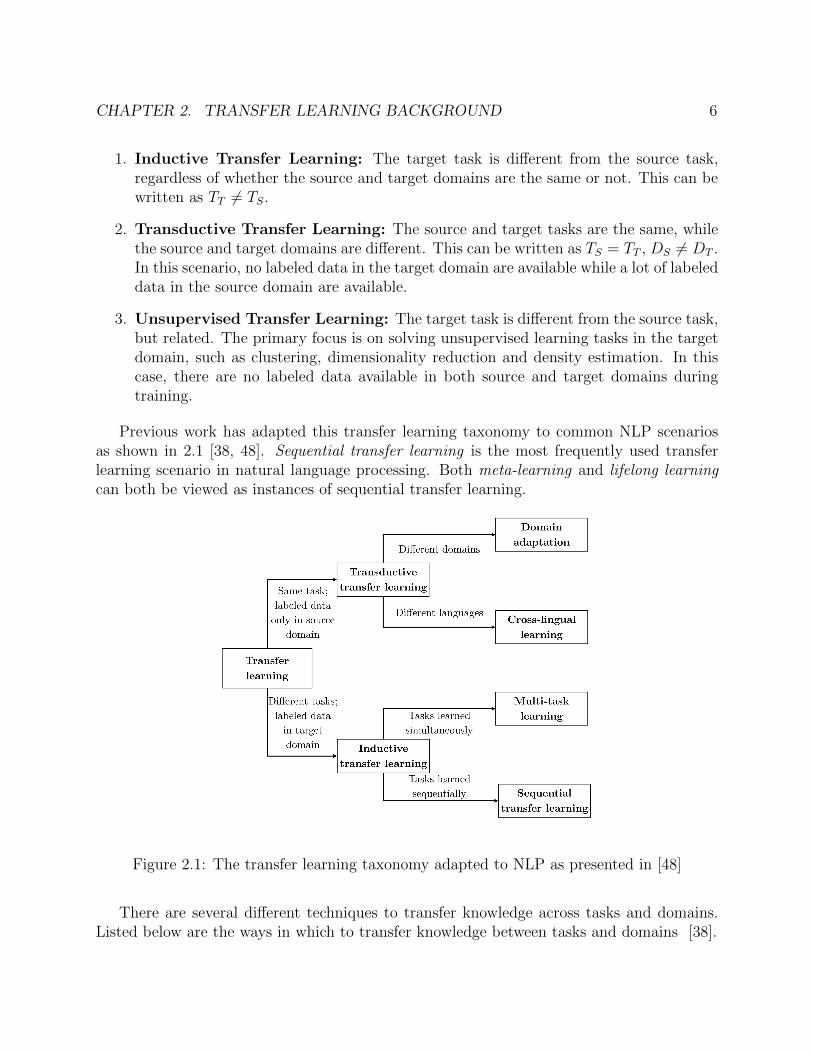
Previous work has adapted this transfer learning taxonomy to common NLP scenariosas shown in 2.1 [38, 48]. Sequential transfer learning is the most frequently used transferlearning scenario in natural language processing. Both meta-learning and lifelong learning
can both be viewed as instances of sequential transfer learning.
Figure 2.1: The transfer learning taxonomy adapted to NLP as presented in [48]
There are several di↵erent techniques to transfer knowledge across tasks and domains.Listed below are the ways in which to transfer knowledge between tasks and domains [38].
CHAPTER 2. TRANSFER LEARNING BACKGROUND 7
1. Instance transfer: Assumes that select data in the source domain can be reused forlearning in the target domain by instance re-weighting and importance sampling [38].
2. Feature-representation transfer: The knowledge used to transfer across domainsis encoded into the learned feature representations; therefore, the goal is to learn a“good” feature representation for the target domain [38].
3. Parameter transfer: The transferred knowledge is encoded into the shared parame-ters or priors [38].
4. Relational-knowledge transfer: Builds mapping of relational knowledge betweenthe source domain and the target domains [38].
In the Natural Language Processing chapter, we primarily focus on sequential transferlearning and domain adaptation through parameter transfer. Within the ReinforcementLearning chapter, we focus on meta-learning techniques and building policies that can adaptto di↵erent environment dynamics.
8
Chapter 3
Handling Unseen Distribution Shift inNLP
3.1 Background
Natural Language Processing is the set of methods for making human language accessibleto computers. Contemporary approaches to natural language processing heavily rely onneural models to build representations of language. Recently, pretraining has emerged asan important technique that leverages large unlabeled corpora to learn universal languagerepresentations; these representations are then fine-tuned to downstream tasks using labeleddata from the target domain.
Pretrained Models
With evolution of deep learning within the past decade, models have rapidly increased inparameter count. These larger models require more data training data to fully learn languagerepresentations; however labeled data tends to be scarce for several NLP tasks such astextual entailment, question answering, document similarity, etc. Building large-scale labeleddatasets is very challenging due to limited resources and expensive annotation costs. On theother hand, unlabeled corpora remains abundant and easily accessible. Pre-training is ableto leverage large corpora through self-supervised learning, which studies the creation of labelsfrom data, by designing ingenious tasks that contain semantic information without humanannotations [22].
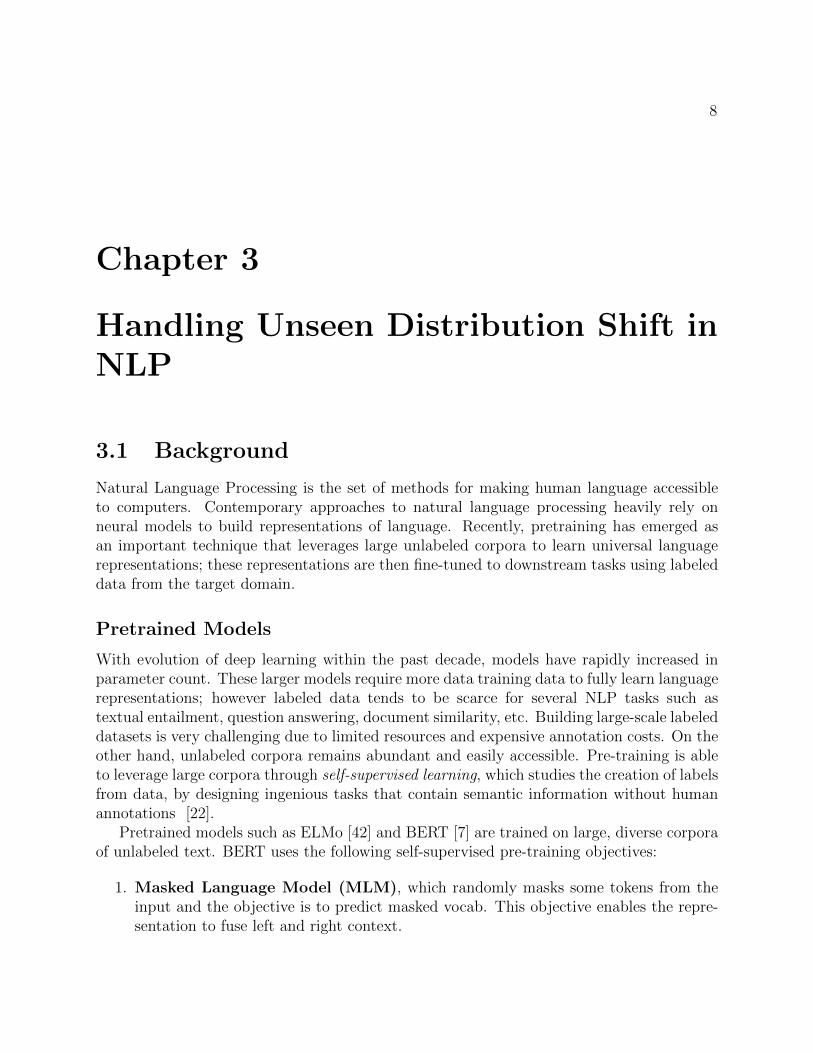
Pretrained models such as ELMo [42] and BERT [7] are trained on large, diverse corporaof unlabeled text. BERT uses the following self-supervised pre-training objectives:
1. Masked Language Model (MLM), which randomly masks some tokens from theinput and the objective is to predict masked vocab. This objective enables the repre-sentation to fuse left and right context.
CHAPTER 3. HANDLING UNSEEN DISTRIBUTION SHIFT IN NLP 9
2. Next Sentence Prediction (NSP), which receives pairs of sentences as input andlearns to predict if the second sentence in the pair is the subsequent sentence in theoriginal document.
BERT’s pre-training corpus consists of BooksCorpus (800M words) [65] and EnglishWikipedia (2,500M words). Since the release of BERT, there have been several domain-specific BERTS developed such as BioBERT (biomedical text) [28], SciBERT (scientificpublications) [1], ClinicalBERT (clinical notes) [24]. These models have been pretrained ona domain specific corpus and yield better performance when fine-tuning them on downstreamNLP tasks for those domains.
Pretrained language models form the foundation of today’s NLP. The representationslearned from these models have achieved state-of-the-art performance across many down-stream tasks with datasets from a diverse set of sources/domains.
Fine-Tuning
After pre-training on large, diverse corpora of unlabeled text, fine-tuning is a techniqueused to adapt the models’ knowledge to downstream tasks. Adapting pretrained models todownstream tasks is a form of transfer learning, which is a means to extract knowledge froma source setting and apply it to a di↵erent target setting [38].
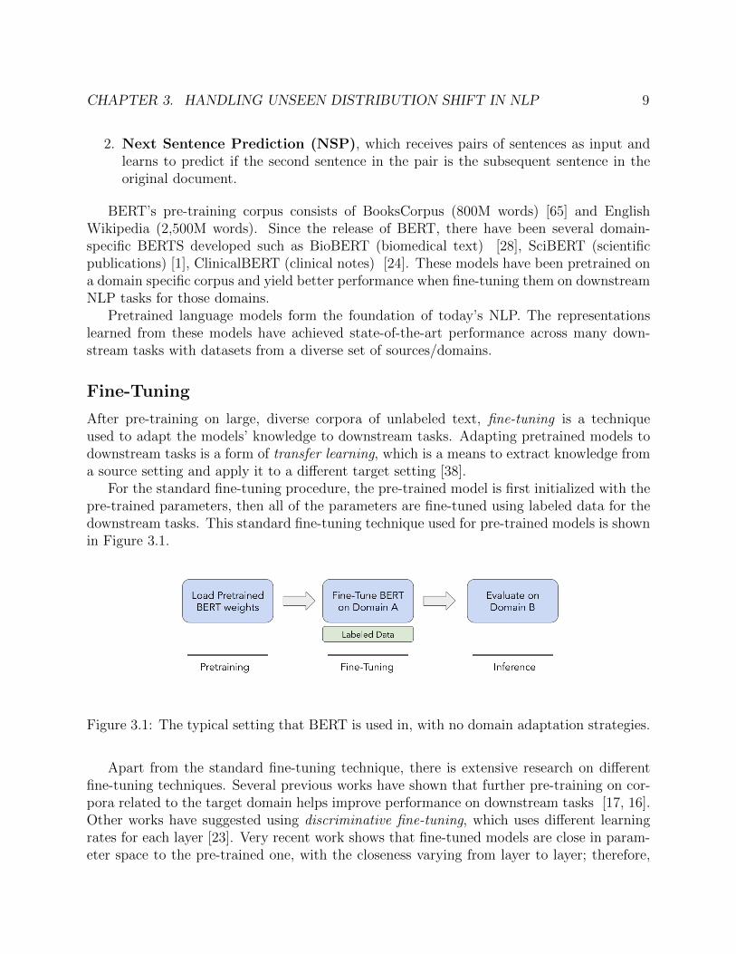
For the standard fine-tuning procedure, the pre-trained model is first initialized with thepre-trained parameters, then all of the parameters are fine-tuned using labeled data for thedownstream tasks. This standard fine-tuning technique used for pre-trained models is shownin Figure 3.1.
Figure 3.1: The typical setting that BERT is used in, with no domain adaptation strategies.
Apart from the standard fine-tuning technique, there is extensive research on di↵erentfine-tuning techniques. Several previous works have shown that further pre-training on cor-pora related to the target domain helps improve performance on downstream tasks [17, 16].Other works have suggested using discriminative fine-tuning, which uses di↵erent learningrates for each layer [23]. Very recent work shows that fine-tuned models are close in param-eter space to the pre-trained one, with the closeness varying from layer to layer; therefore,
CHAPTER 3. HANDLING UNSEEN DISTRIBUTION SHIFT IN NLP 10
it su�ces to fine-tune only the most critical layers [44]. In this chapter, we run severalexperiments in order to understand and interpret what happens to language representationsduring and after fine-tuning.
Evaluation on Downstream Tasks
The General Language Understanding Evaluation (GLUE) benchmark [60] is a collectionof nine natural language understanding tasks, including single-sentence classification tasks(CoLA and SST-2), pairwise text classification tasks (MNLI, RTE,WNLI, QQP, and MRPC),text similarity task (STS-B), and relevant ranking task (QNLI). The GLUE benchmark servesas a metric to compare di↵erent pre-trained models. In this chapter, we evaluate our methodson a variety of tasks using several diverse datasets.
3.2 Approach
We explore a new setting in which the domain of the examples received during test-timeis unknown; in other words, there is no data available during training-time to anticipatedistribution shifts. We propose a technique to adapt to unforeseeable domain/distributionshifts during test-time. Upon receiving an example from an unfamiliar domain during test-time, we believe the language model will greatly benefit from additional training (or fine-tuning) on the test example and other similar, relevant examples using the unsupervisedmasked language modeling objective. By taking gradient step(s) using an labeled objectiveon the test-example, the model is able to get practice reading the domain and makingpredictions before actually testing; this is very similar to how humans approach learning.Using test-time training for out-of-distribution generalization has been studied in computervision [56]; however, these ideas have several unique applications for NLP.
In order for auxiliary tasks to be helpful for the primary task, the tasks must sharesimilarities. One way to measure task similarity is to compute the cosine similarity betweenthe gradients of the tasks [8]. Our test-time training approach only works if the gradientsfrom the masked language modeling objective are roughly aligned with the gradients of thesupervised objective. To this end, we propose a gradient alignment technique to explicitlytrain a model such that the gradients from the masked language modeling objective and thesupervised objective is aligned.
We evaluate our approach on a variety of di↵erent tasks such as sentiment analysis,textual entailment, and semantic similarity.
Test-time Training
Test-time training for out-of-distribution generalization was first introduced for computervision models [56]. Let xi be an unlabeled example received at test time. Although we donot know the domain of example xi, we can use information about xi in order to update the
CHAPTER 3. HANDLING UNSEEN DISTRIBUTION SHIFT IN NLP 11
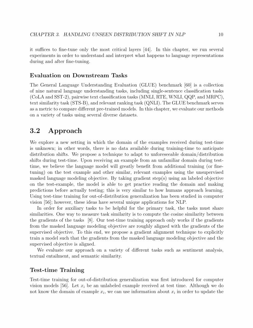
Figure 3.2: This is our test-time training approach for the setting in which the domain of theexamples at test-time is unknown. Upon receiving an example at test time, we take gradientsteps on similar examples, make the prediction, then reset the weights before receiving thenext example during inference.
parameters before making a prediction yi. In this test-time training approach, the modelparameters ✓ depend on the test instance x, but not its unknown label y.
In order to update the parameters ✓ at test time, we can create a self-supervised learningproblem from the test instance x. Self-supervised learning is a technique that automaticallycreates labels from unlabeled inputs using an auxiliary task. Specifically, we can use themasked language modeling (MLM) objective over unlabeled text. In addition to using testinstance x for test-time training, we can also retrieve similar examples from the trainingcorpus. By taking gradient steps on similar examples during test-time, the model will beable to get practice reading a domain before making predictions.
In the online setting, we receive examples sequentially, one at a time. In the settingwhere the examples arrive in batches, we can perform test-time training using the batcheddata.
Parameter Resetting. After making a prediction for each example during test-time,we consider whether the parameters should be rewound to the parameters attained after fine-tuning. Not resetting the parameters may cause the model to drift away from the sourcedomain, which is known as catastrophic forgetting [34]. On the other hand, if we know thatwe will receive a series of inputs from a certain domain, then it may be beneficial to keepupdating the model without resetting parameters. In this report, we perform all test-timetraining experiments by resetting the model parameters after each example at test time.
Computational E�ciency. One downside to test-time training is that it increasescompute, since additional forward and backward passes are required during inference. Inorder to reduce compute, we can only take gradient steps on examples that appear to beout-of-distribution. A simple baseline for out-of-distribution detection would be to set athreshold in the output confidence. This is something we save for future work.
CHAPTER 3. HANDLING UNSEEN DISTRIBUTION SHIFT IN NLP 12
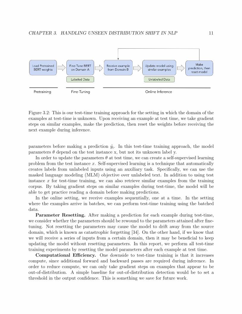
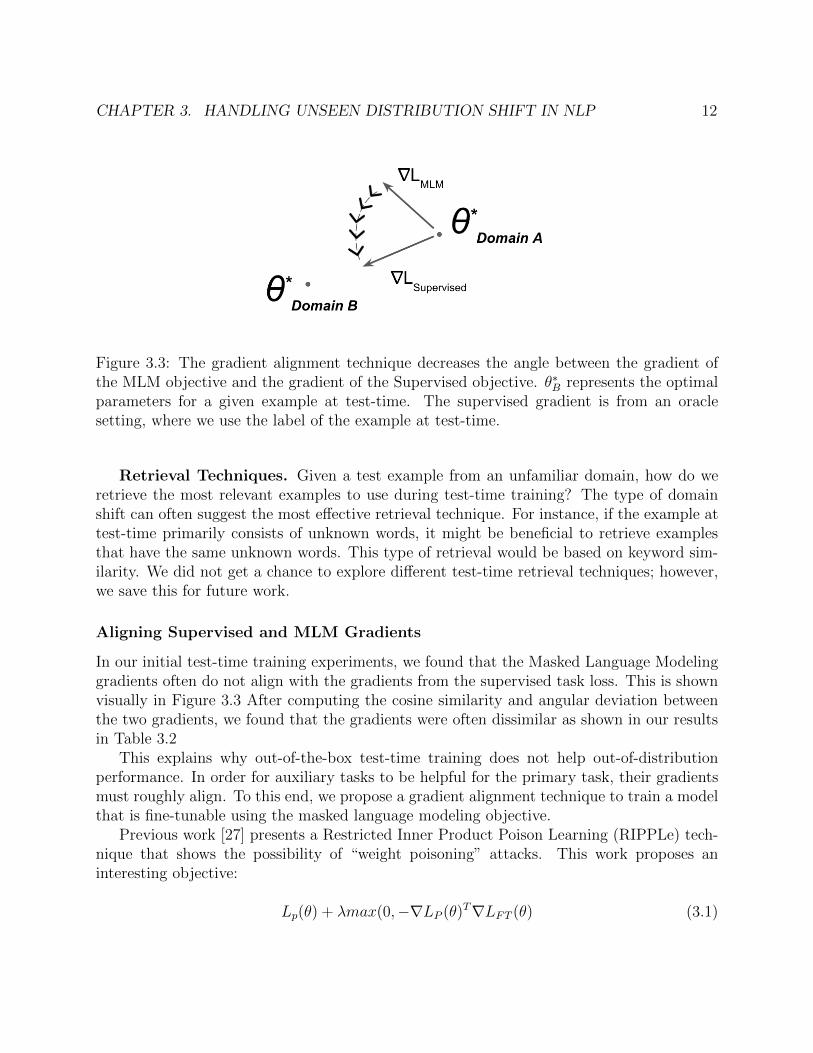
Figure 3.3: The gradient alignment technique decreases the angle between the gradient ofthe MLM objective and the gradient of the Supervised objective. ✓⇤B represents the optimalparameters for a given example at test-time. The supervised gradient is from an oraclesetting, where we use the label of the example at test-time.
Retrieval Techniques. Given a test example from an unfamiliar domain, how do weretrieve the most relevant examples to use during test-time training? The type of domainshift can often suggest the most e↵ective retrieval technique. For instance, if the example attest-time primarily consists of unknown words, it might be beneficial to retrieve examplesthat have the same unknown words. This type of retrieval would be based on keyword sim-ilarity. We did not get a chance to explore di↵erent test-time retrieval techniques; however,we save this for future work.
Aligning Supervised and MLM Gradients
In our initial test-time training experiments, we found that the Masked Language Modelinggradients often do not align with the gradients from the supervised task loss. This is shownvisually in Figure 3.3 After computing the cosine similarity and angular deviation betweenthe two gradients, we found that the gradients were often dissimilar as shown in our resultsin Table 3.2
This explains why out-of-the-box test-time training does not help out-of-distributionperformance. In order for auxiliary tasks to be helpful for the primary task, their gradientsmust roughly align. To this end, we propose a gradient alignment technique to train a modelthat is fine-tunable using the masked language modeling objective.
Previous work [27] presents a Restricted Inner Product Poison Learning (RIPPLe) tech-nique that shows the possibility of “weight poisoning” attacks. This work proposes aninteresting objective:
Lp(✓) + �max(0,�rLP (✓)TrLFT (✓) (3.1)
CHAPTER 3. HANDLING UNSEEN DISTRIBUTION SHIFT IN NLP 13
The second regularization term encourages the inner product between the poisoning lossgradient and the fine tuning loss gradient to be non-negative. This objective function inspiredus to construct a meta-learning objective that trains the model to be fine tunable using themasked language modeling loss at test time. Let LSV be the supervised loss and LMLM bethe masked language modeling loss. We propose the following objective:
LSV (✓)� �rLMLM(✓)TrLSV (✓)
krLMLMkkrLSV k(3.2)
The objective above can also be written in terms of the cosine similarity between thegradient vectors:
LSV (✓)� �cos(�) (3.3)
where � represents the angle between the Supervised gradient and the MLM gradient and� represents the strength of the regularization. Rather than encouraging the model to learnparameters such that the gradients to have a high dot product, we instead normalize thegradient vectors. This prevents the model from increasing the norm of the gradients in orderto decrease the loss.
3.3 Experiments
We use the BERT Base model [7] in our experiments. Note that our approach is agnostic tothe underlying pretrained model.
Train and Test Datasets
We evaluate generalization using a variety of tasks and data sources. We utilize two sentimentanalysis datasets:
• We use the SST-2 Dataset, which contains formal movie reviews labeled with theirsentiment [54]. We also use the IMDb dataset [30], which is also a binary sentimentanalysis dataset containing of informal reviews
• The Amazon Review Dataset contains product reviews from Amazon [33, 18].We primarily focused on the categories that had larger generalization gaps in [21].We collected data from a few clothing categories (Women Clothing, Mens Clothing,Baby Clothing, Shoes) and two categories of entertainment products (Movies, Music).Models predict a review’s 1 to 5 star rating, and we report accuracy.
We utilize the following datasets for semantic similarity, entity span identification and part-of-speech tagging tasks:
CHAPTER 3. HANDLING UNSEEN DISTRIBUTION SHIFT IN NLP 14
• The STS-B Dataset requires predicting the semantic similarity between pairs ofsentences [3]. The dataset contains text of di↵erent genres and sources; we use foursources from two genres: Microsoft Research Paraphrase Corpus (MSRpar) (news),Headlines (news); MSRvid (captions), Images (captions). The evaluation metric isPearson’s correlation coe�cient.
• The canonicalConference on Natural Language Learning (CoNLL) 2003 sharedtask dataset contains named entity spans that were annotated on a corpus of new-stext [50]. After training on the CoNLL dataset, we focus on identifying named entityspans in Tweets, which was the shared task of the 2016 Workshop on Noisy UserText [55].
• The Penn Parsed Corpora of Historical English (PPCHE) contains part-of-speech annotations for texts originating from several historical periods [26]. We pri-marily focus on the corpus that covers Early Modern English, which we refer to asPPCEME. Due to the limited access of this dataset, we were not able to run exper-iments in time for this report; however, in the coming weeks, we will train on thePenn Treebank (PTB) corpus of 20th century English [32], and then evaluate onthe PPCEME test set.
We chose these tasks and datasets because they represent realistic distribution shifts andare used in past work [21, 17].
Tools
We used PyTorch [40] along with the Hugging Face Transformers library [62] in orderto run our experiments. The Hugging Face Transformers library provides saved modelscheckpoints for numerous pretrained models; we load the o�cial pre-trained BERT weightsfor our experiments. We also used Jupyter Notebooks and Pandas for data cleaning andvisualization. In order to run experiments, we used the RISE machines with GPUs alongwith the Slurm Workload Manager to schedule jobs.
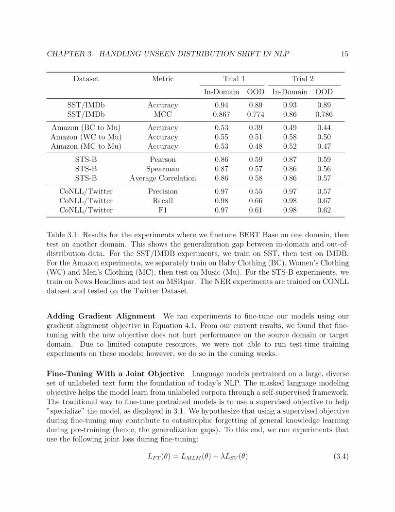
Natural Robustness of BERT We investigate the natural ability of the BERT-Basemodel to generalize to out-of-distribution examples; our experiment results are listed inTable 3.1. These experiments form a baseline/reference for comparing the experiments thatuse our domain adaptation techniques.
Robustness with Test-Time Adaptation We perform our test-time adaptation ap-proach by a taking gradient step We found that test-time training alone does not signifi-cantly help performance as shown in our results in Table 3.2. Even after running additionaltest-time training experiments using more gradient steps and more examples, we found thatusing the masked language modeling objective is not helpful at test-time, since it does notalign with the true supervised objective (in terms of their gradients).
CHAPTER 3. HANDLING UNSEEN DISTRIBUTION SHIFT IN NLP 15
Dataset Metric Trial 1 Trial 2
In-Domain OOD In-Domain OOD
SST/IMDb Accuracy 0.94 0.89 0.93 0.89SST/IMDb MCC 0.867 0.774 0.86 0.786
Amazon (BC to Mu) Accuracy 0.53 0.39 0.49 0.44Amazon (WC to Mu) Accuracy 0.55 0.51 0.58 0.50Amazon (MC to Mu) Accuracy 0.53 0.48 0.52 0.47
STS-B Pearson 0.86 0.59 0.87 0.59STS-B Spearman 0.87 0.57 0.86 0.56STS-B Average Correlation 0.86 0.58 0.86 0.57
CoNLL/Twitter Precision 0.97 0.55 0.97 0.57CoNLL/Twitter Recall 0.98 0.66 0.98 0.67CoNLL/Twitter F1 0.97 0.61 0.98 0.62
Table 3.1: Results for the experiments where we finetune BERT Base on one domain, thentest on another domain. This shows the generalization gap between in-domain and out-of-distribution data. For the SST/IMDB experiments, we train on SST, then test on IMDB.For the Amazon experiments, we separately train on Baby Clothing (BC), Women’s Clothing(WC) and Men’s Clothing (MC), then test on Music (Mu). For the STS-B experiments, wetrain on News Headlines and test on MSRpar. The NER experiments are trained on CONLLdataset and tested on the Twitter Dataset.
Adding Gradient Alignment We ran experiments to fine-tune our models using ourgradient alignment objective in Equation 4.1. From our current results, we found that fine-tuning with the new objective does not hurt performance on the source domain or targetdomain. Due to limited compute resources, we were not able to run test-time trainingexperiments on these models; however, we do so in the coming weeks.
Fine-Tuning With a Joint Objective Language models pretrained on a large, diverseset of unlabeled text form the foundation of today’s NLP. The masked language modelingobjective helps the model learn from unlabeled corpora through a self-supervised framework.The traditional way to fine-tune pretrained models is to use a supervised objective to help”specialize” the model, as displayed in 3.1. We hypothesize that using a supervised objectiveduring fine-tuning may contribute to catastrophic forgetting of general knowledge learningduring pre-training (hence, the generalization gaps). To this end, we run experiments thatuse the following joint loss during fine-tuning:
LFT (✓) = LMLM(✓) + �LSV (✓) (3.4)
CHAPTER 3. HANDLING UNSEEN DISTRIBUTION SHIFT IN NLP 16
Dataset Trial 1 Trial 2
Cosine Sim. Angle OOD Acc. Cosine Sim. Angle OOD Acc.
SST/IMDb �0.16 94.65 0.87 �0.19 102.46 0.88
STS-B �0.20 125.46 - �0.19 126.38 -
Amazon (WC/Mu) 0.01 104.46 0.51 �0.01 100.91 0.52
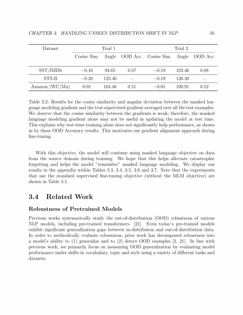
Table 3.2: Results for the cosine similarity and angular deviation between the masked lan-guage modeling gradient and the true supervised gradient averaged over all the test examples.We observe that the cosine similarity between the gradients is weak; therefore, the maskedlanguage modeling gradient alone may not be useful in updating the model at test time.This explains why test-time training alone does not significantly help performance, as shownin by these OOD Accuracy results. This motivates our gradient alignment approach duringfine-tuning.
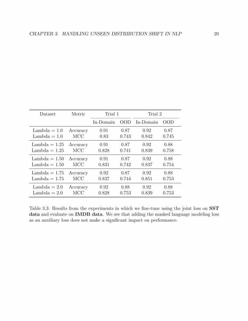
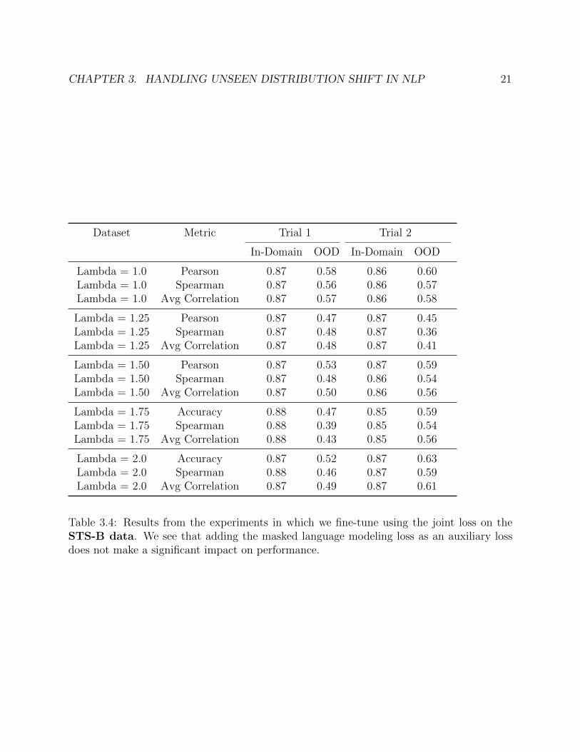
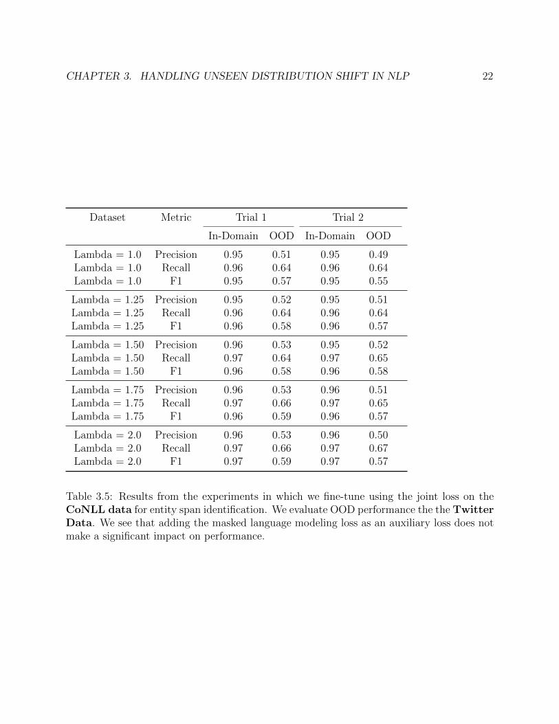
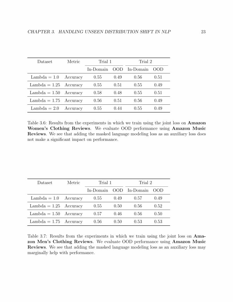
With this objective, the model will continue using masked language objective on datafrom the source domain during training. We hope that this helps alleviate catastrophicforgetting and helps the model ”remember” masked language modeling. We display ourresults in the appendix within Tables 3.3, 3.4, 3.5, 3.6 and 3.7. Note that the experimentsthat use the standard supervised fine-tuning objective (without the MLM objective) areshown in Table 3.1.
3.4 Related Work
Robustness of Pretrained Models
Previous works systematically study the out-of-distribution (OOD) robustness of variousNLP models, including pre-trained transformers [21]. Even today’s pre-trained modelsexhibit significant generalization gaps between in-distributon and out-of-distribution data.In order to methodically evaluate robustness, prior work has decomposed robustness intoa model’s ability to (1) generalize and to (2) detect OOD examples [2, 21]. In line withprevious work, we primarily focus on measuring OOD generalization by evaluating modelperformance under shifts in vocabulary, topic and style using a variety of di↵erent tasks anddatasets.
CHAPTER 3. HANDLING UNSEEN DISTRIBUTION SHIFT IN NLP 17
Domain Adaptation Techniques
Domain adaptation is an important problem in NLP and has been well studied in recentyears. There is an expansive set of work domain adaptation studies that have focused ontasks such as sentiment analysis [14, 53], paraphrase detection [52], and Part-Of-Speech(POS) tagging.
Unsupervised Domain Adaptation
One particular line of work this unsupervised domain adaptation (transfer learning), whichstudies the problem of distribution shift (from P to Q), when unlabeled data from Q isavailable at training-time. Some NLP research in unsupervised domain adaptation has shownimproved performance when fine-tuning the pre-trained models using unlabeled data fromthe target domain (e.g., [17, 16]), as shown in Figure 3.4. Although this fine-tuning improvesperformance, it requires knowledge of the target domain during training; this knowledge isnot available in our setting. Therefore, we view this as the upper bound on performance,since the model is specialized for the target domain during training. The lower bound onperformance is when the model is trained on an entirely di↵erent domain than the targetdomain (with no additional fine-tuning on the target domain). Our work attempts to closethe gap between these two bounds, given no prior information about the target domain attest-time.
Supervised Domain Adaptation
Other research has proposed techniques that use labeled data from the target domain duringfine-tuning. Most of these studies assume that there is prior knowledge about the distributionshift available during training; this assumption di↵erentiates our work from most prior workin domain adaptation.
Computer Vision Parallels
Transfer learning has been heavily used in computer vision; instead of building a model fromscratch, we can start with a model pre-trained on ImageNet.
We were inspired by many of the unsupervised domain adaptation techniques explored incomputer vision [59, 13, 5]. We also took inspiration from recent computer vision researchin self-supervised learning, which studies the creation of labels from data, by designingingenious tasks that contain semantic information without human annotations [22]. In fact,test-time training was originally explored in computer vision [56], which inspired our ownapproach in the NLP setting.
CHAPTER 3. HANDLING UNSEEN DISTRIBUTION SHIFT IN NLP 18
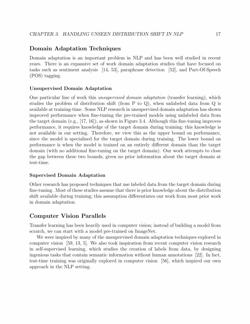
Figure 3.4: The approach used in [17] when we know the domain received at test time. Inorder to adapt to out-of-distribution examples, this technique performs a domain-tuning stepusing unlabeled data from domain B. Next, a task-tuning step is performed using unlabeleddata on Domain A.
Auxiliary Losses
Much of recent work has explored the use of auxiliary losses to help improve data e�ciencyand build useful representations. Auxiliary tasks have been proven to work well in prac-tice [25, 64, 35, 39]; however, the e�cacy of an auxiliary task depends on the similaritybetween an auxiliary task and the main task of interest. A previous work [8] proposes usingcosine similarity of gradients between tasks as a generalizable measure of task similarity.Using the cosine similarity metric, we evaluate the e↵ectiveness of the masked languagemodeling auxiliary task for test-time training. Furthermore, we propose a gradient align-ment technique in order to train the model to be fine tunable using the MLM loss at testtime. Our technique is reminiscent of Model-Agnostic Meta-Learning (MAML), which is analgorithm to help networks to quickly adapt to new tasks [12].
Pre-Training and Self-Supervision
Very early work has shown the e�cacy of pretraining. Prior work found that using unlabeleddata from related tasks in the pre-training can improve the generalization of a subsequentsupervised model [6]. These results demonstrate that one can use unsupervised learning withmore unlabeled data to improve supervised learning; this result helped build the foundationof today’s NLP. Given this result, we aim to explore ways to leverage unlabeled data duringthe fine-tuning step to help the model generalize to out-of-distribution data.
CHAPTER 3. HANDLING UNSEEN DISTRIBUTION SHIFT IN NLP 19
Previous research demonstrates that self-supervision can greatly improves robustness anduncertainty [20]. Although self-supervision may not substantially improve accuracy whenused with standard training on labeled datasets, it has been shown to improve several aspectsof model robustness, including robustness to adversarial examples [31], label corruptions[41], and common input corruptions [19]. These findings motivate the idea of using maskedlanguage modeling loss (in addition to supervised loss) when fine-tuning language models.The standard fine-tuning technique used for pre-trained models is shown in Figure 3.1.
Understanding Fine-Tuning
Prior research explores the inductive transfer learning setting for NLP using the languagemodeling objective [38]. Previous work introduced Universal Language Model Finetuning(ULMFiT), which pretrains a language model on a large general-domain corpus and fine-tunes it on the target task using novel techniques [23].
3.5 Conclusion and Future Work
Since distribution shifts are often unforeseen in practice, models must adapt on-the-fly attest-time. We presented a test-time training technique that leverages unsupervised infor-mation from the test example and similar training examples to adapt NLP models. Weexplicitly optimize the auxiliary MLM loss to be helpful during test-time training by opti-mizing the loss’ gradient to be aligned with the supervised loss. We evaluated our techniquesusing several di↵erent tasks and datasets
In ongoing work, we will continue to evaluate our approach, as well as study how train-ing with MLM loss during fine-tuning changes both in-distribution and out-of-distributionperformance. It would also be interesting to study the e↵ect of fine-tuning on the MLM lossof in-domain and OOD examples. This would help understand what fine-tuning is exactlydoing to the embeddings.
CHAPTER 3. HANDLING UNSEEN DISTRIBUTION SHIFT IN NLP 20
Dataset Metric Trial 1 Trial 2
In-Domain OOD In-Domain OOD
Lambda = 1.0 Accuracy 0.91 0.87 0.92 0.87Lambda = 1.0 MCC 0.83 0.743 0.842 0.745
Lambda = 1.25 Accuracy 0.91 0.87 0.92 0.88Lambda = 1.25 MCC 0.828 0.741 0.839 0.758
Lambda = 1.50 Accuracy 0.91 0.87 0.92 0.88Lambda = 1.50 MCC 0.831 0.742 0.837 0.754
Lambda = 1.75 Accuracy 0.92 0.87 0.92 0.88Lambda = 1.75 MCC 0.837 0.744 0.851 0.753
Lambda = 2.0 Accuracy 0.92 0.88 0.92 0.88Lambda = 2.0 MCC 0.828 0.753 0.839 0.753
Table 3.3: Results from the experiments in which we fine-tune using the joint loss on SSTdata and evaluate on IMDB data. We see that adding the masked language modeling lossas an auxiliary loss does not make a significant impact on performance.
CHAPTER 3. HANDLING UNSEEN DISTRIBUTION SHIFT IN NLP 21
Dataset Metric Trial 1 Trial 2
In-Domain OOD In-Domain OOD
Lambda = 1.0 Pearson 0.87 0.58 0.86 0.60Lambda = 1.0 Spearman 0.87 0.56 0.86 0.57Lambda = 1.0 Avg Correlation 0.87 0.57 0.86 0.58
Lambda = 1.25 Pearson 0.87 0.47 0.87 0.45Lambda = 1.25 Spearman 0.87 0.48 0.87 0.36Lambda = 1.25 Avg Correlation 0.87 0.48 0.87 0.41
Lambda = 1.50 Pearson 0.87 0.53 0.87 0.59Lambda = 1.50 Spearman 0.87 0.48 0.86 0.54Lambda = 1.50 Avg Correlation 0.87 0.50 0.86 0.56
Lambda = 1.75 Accuracy 0.88 0.47 0.85 0.59Lambda = 1.75 Spearman 0.88 0.39 0.85 0.54Lambda = 1.75 Avg Correlation 0.88 0.43 0.85 0.56
Lambda = 2.0 Accuracy 0.87 0.52 0.87 0.63Lambda = 2.0 Spearman 0.88 0.46 0.87 0.59Lambda = 2.0 Avg Correlation 0.87 0.49 0.87 0.61
Table 3.4: Results from the experiments in which we fine-tune using the joint loss on theSTS-B data. We see that adding the masked language modeling loss as an auxiliary lossdoes not make a significant impact on performance.
CHAPTER 3. HANDLING UNSEEN DISTRIBUTION SHIFT IN NLP 22
Dataset Metric Trial 1 Trial 2
In-Domain OOD In-Domain OOD
Lambda = 1.0 Precision 0.95 0.51 0.95 0.49Lambda = 1.0 Recall 0.96 0.64 0.96 0.64Lambda = 1.0 F1 0.95 0.57 0.95 0.55
Lambda = 1.25 Precision 0.95 0.52 0.95 0.51Lambda = 1.25 Recall 0.96 0.64 0.96 0.64Lambda = 1.25 F1 0.96 0.58 0.96 0.57
Lambda = 1.50 Precision 0.96 0.53 0.95 0.52Lambda = 1.50 Recall 0.97 0.64 0.97 0.65Lambda = 1.50 F1 0.96 0.58 0.96 0.58
Lambda = 1.75 Precision 0.96 0.53 0.96 0.51Lambda = 1.75 Recall 0.97 0.66 0.97 0.65Lambda = 1.75 F1 0.96 0.59 0.96 0.57
Lambda = 2.0 Precision 0.96 0.53 0.96 0.50Lambda = 2.0 Recall 0.97 0.66 0.97 0.67Lambda = 2.0 F1 0.97 0.59 0.97 0.57
Table 3.5: Results from the experiments in which we fine-tune using the joint loss on theCoNLL data for entity span identification. We evaluate OOD performance the the TwitterData. We see that adding the masked language modeling loss as an auxiliary loss does notmake a significant impact on performance.
CHAPTER 3. HANDLING UNSEEN DISTRIBUTION SHIFT IN NLP 23
Dataset Metric Trial 1 Trial 2
In-Domain OOD In-Domain OOD
Lambda = 1.0 Accuracy 0.55 0.49 0.56 0.51
Lambda = 1.25 Accuracy 0.55 0.51 0.55 0.49
Lambda = 1.50 Accuracy 0.58 0.48 0.55 0.51
Lambda = 1.75 Accuracy 0.56 0.51 0.56 0.49
Lambda = 2.0 Accuracy 0.55 0.44 0.55 0.49
Table 3.6: Results from the experiments in which we train using the joint loss on AmazonWomen’s Clothing Reviews. We evaluate OOD performance using Amazon MusicReviews. We see that adding the masked language modeling loss as an auxiliary loss doesnot make a significant impact on performance.
Dataset Metric Trial 1 Trial 2
In-Domain OOD In-Domain OOD
Lambda = 1.0 Accuracy 0.55 0.49 0.57 0.49
Lambda = 1.25 Accuracy 0.55 0.50 0.56 0.52
Lambda = 1.50 Accuracy 0.57 0.46 0.56 0.50
Lambda = 1.75 Accuracy 0.56 0.50 0.53 0.53
Table 3.7: Results from the experiments in which we train using the joint loss on Ama-zon Men’s Clothing Reviews. We evaluate OOD performance using Amazon MusicReviews. We see that adding the masked language modeling loss as an auxiliary loss maymarginally help with performance.
24
Chapter 4
Improving Generalization in RLThrough Better Adaptation
4.1 Background
Reinforcement learning (RL) studies algorithms for sequential decision problems, where anagent learns to maximize cumulative reward by interacting with its environment. The re-inforcement learning setting can be formulated as a Markov Decision Process (MDP) withstates S, actions A, transitions T , rewards r, and discount factor �. Given that an agent is instate s and takes action a, the probability that the agent lands in a new state s0 is T (s, a, s0).The objective of RL is to learn a policy ⇡(a|s) that, given a state, outputs the probabilitydistribution over the next action the agent should take to maximize its cumulative reward.
In recent years, deep RL has eliminated the need to hand-engineer features for RL policies.Using deep neural networks has enabled reinforcement learning algorithms to solve complexproblems end-to-end.
Meta Learning
The success of deep learning heavily relies on the availability of vast amount of labeled data.Current ML/AI systems can learn a complex skill or task very well in a fixed environment,given a large amount of time/experience; however, it is impractical to train each skill in eachsetting in isolation. Instead of considering each new task in isolation, agents should be able toquickly learn new tasks by reusing previous experience. This crucial ability to adapt not onlyenables agents to pick up new skills/tasks faster, but also helps agents handle unexpectedperturbations or unseen situations at test time. This is the approach of meta-learning, orlearning to learn.
Meta-learning algorithms leverage data from previous tasks to develop a learning proce-dure that can quickly adapt to new tasks. During meta-learning, the model is trained tolearn multiple tasks in the meta-training set; these tasks are referred to as meta-training
tasks. Meta-learning techniques assume that the previous meta-training tasks and the new
CHAPTER 4. IMPROVING GENERALIZATION IN RL THROUGH BETTERADAPTATION 25
meta-test tasks are drawn from the same task distribution and share similarities that canbe exploited for fast learning. In this meta-learning approach, there exist two layers of op-timization at play – the learner, which learns new tasks, and the meta-learner, which trainsthe learner.
Meta-learning is a key stepping stone towards versatile agents that can continuallyadapt and learn a wide variety of tasks throughout their lifetimes. A few common ap-proaches to meta-learning within reinforcement learning are optimization-based approachesand recurrence-based approaches.
Optimization-Based Meta-Learning.
Standard deep learning models learn by computing gradients through backpropogation;however, this is not designed to be e↵ective with a small number of training examples.Furthermore, it is not guaranteed to converge within few optimization steps. Therefore,optimization-based meta-learning adjusts the optimization algorithm so that the model canlearn new tasks using a few examples.
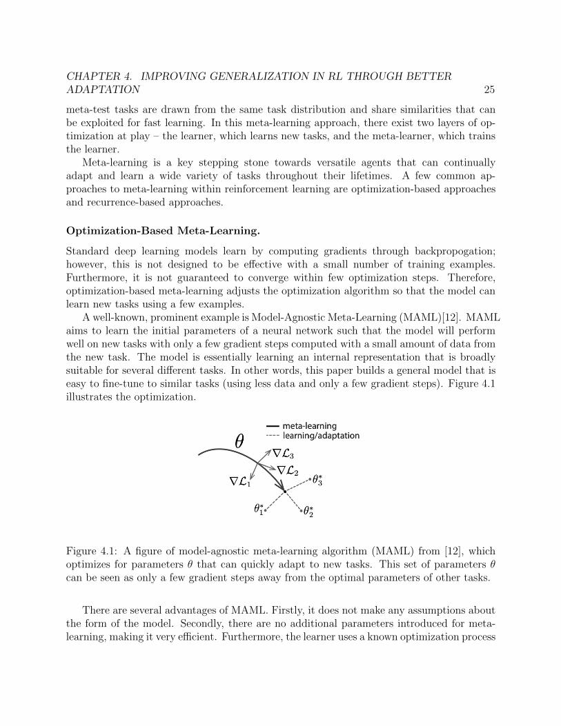
A well-known, prominent example is Model-Agnostic Meta-Learning (MAML)[12]. MAMLaims to learn the initial parameters of a neural network such that the model will performwell on new tasks with only a few gradient steps computed with a small amount of data fromthe new task. The model is essentially learning an internal representation that is broadlysuitable for several di↵erent tasks. In other words, this paper builds a general model that iseasy to fine-tune to similar tasks (using less data and only a few gradient steps). Figure 4.1illustrates the optimization.
Figure 4.1: A figure of model-agnostic meta-learning algorithm (MAML) from [12], whichoptimizes for parameters ✓ that can quickly adapt to new tasks. This set of parameters ✓can be seen as only a few gradient steps away from the optimal parameters of other tasks.
There are several advantages of MAML. Firstly, it does not make any assumptions aboutthe form of the model. Secondly, there are no additional parameters introduced for meta-learning, making it very e�cient. Furthermore, the learner uses a known optimization process
CHAPTER 4. IMPROVING GENERALIZATION IN RL THROUGH BETTERADAPTATION 26
(gradient descent). It can also be applied to several domains such as regression, classification,and reinforcement learning.
Recurrence-Based Meta-Learning.
Another approach to meta-learning is to use recurrent models (ie. RNN, LSTM, etc.). Therecurrent model processes inputs sequentially and produces outputs at each timestep.
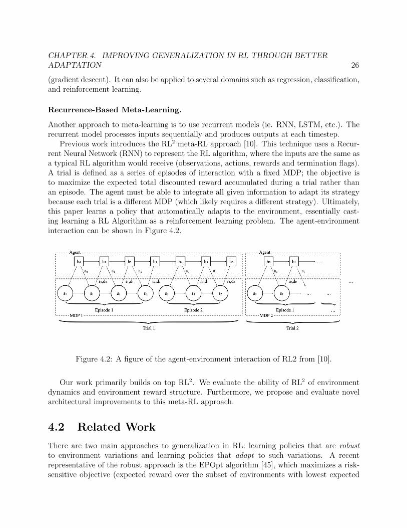
Previous work introduces the RL2 meta-RL approach [10]. This technique uses a Recur-rent Neural Network (RNN) to represent the RL algorithm, where the inputs are the same asa typical RL algorithm would receive (observations, actions, rewards and termination flags).A trial is defined as a series of episodes of interaction with a fixed MDP; the objective isto maximize the expected total discounted reward accumulated during a trial rather thanan episode. The agent must be able to integrate all given information to adapt its strategybecause each trial is a di↵erent MDP (which likely requires a di↵erent strategy). Ultimately,this paper learns a policy that automatically adapts to the environment, essentially cast-ing learning a RL Algorithm as a reinforcement learning problem. The agent-environmentinteraction can be shown in Figure 4.2.
Figure 4.2: A figure of the agent-environment interaction of RL2 from [10].
Our work primarily builds on top RL2. We evaluate the ability of RL2 of environmentdynamics and environment reward structure. Furthermore, we propose and evaluate novelarchitectural improvements to this meta-RL approach.
4.2 Related Work
There are two main approaches to generalization in RL: learning policies that are robust
to environment variations and learning policies that adapt to such variations. A recentrepresentative of the robust approach is the EPOpt algorithm [45], which maximizes a risk-sensitive objective (expected reward over the subset of environments with lowest expected
CHAPTER 4. IMPROVING GENERALIZATION IN RL THROUGH BETTERADAPTATION 27
reward). Adversarial training has also been proposed to learn a robust policy [43]. A keyweakness of robust policies is that they may sacrifice performance on many environmentvariants in order to avoid failing on a few.
Lately there has been increased interest in learning policies that can adapt to the envi-ronment at hand. A number of algorithms learn embeddings for each environment variantas a function of trajectories sampled from that environment, which are utilized by the agent.Previous work presents model-free methods, letting the embedding be input into a policyand/or value function [10, 61, 58, 36, 46]. In contrast, other previous research [4, 49] aremodel-based methods, where the embedding is input into a dynamics model and actions areselected using model predictive control. Other works [11] and [47] (and many other exten-sions) present a meta-learning formulation of generalization in RL, training a policy thatcan be updated with good data e�ciency for each test environment.
Our work primarily builds upon the architecture and training setup presented in the RL2
work [10]. RL2 aims to train an agent that can adapt to the dynamics of the environmentat hand. RL2 models the policy and value functions as a recurrent neural network (RNN)with the current trajectory as input, not just the sequence of states; the hidden states ofthe RNN may be viewed as an embedding of the environment. Specifically, for the RNNthe inputs at time t are st, at�1, rt�1, and dt�1, where dt�1 is a Boolean variable indicatingwhether the episode ended after taking action at�1; the hidden states are updated and atis output. At each iteration trajectories are generated using the current policy with theenvironment state reset at the end of each episode. The hidden states of the policy are resetand a new environment is sampled from q only at the end of every N episodes, which is calleda trial. The generated trajectories are then input into some policy-based RL algorithm thatmaximizes the expected reward in a trial (TRPO in the paper, and PPO in open-sourcedbaselines and in our own implementation).
4.3 Approach
Meta-RL Robots
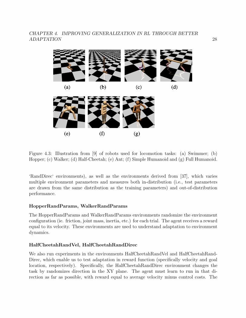
We evaluate our methods on various locomotion tasks, which are widely analyzed in rein-forcement learning and control literature. Figure 4.3 illustrates six common robots used forlocomotion tasks [9]. In general, performing tasks using these robots is more challengingthan other basic tasks/robots due to high degrees of freedom. We primarily use the Hopper,Walker and HalfCheetah robots.
Meta-RL Environment Specifications
Recent meta-RL approaches such as PEARL [46] and ProMP [47] have studied the adaptationof agents to changes in environment dynamics. We evaluate our approach on the becnhmarkenvironments considered in PEARL and ProMP (i.e., the ‘RandParams‘, ‘RandVel‘, and
CHAPTER 4. IMPROVING GENERALIZATION IN RL THROUGH BETTERADAPTATION 28
Figure 4.3: Illustration from [9] of robots used for locomotion tasks: (a) Swimmer; (b)Hopper; (c) Walker; (d) Half-Cheetah; (e) Ant; (f) Simple Humanoid and (g) Full Humanoid.
‘RandDirec‘ environments), as well as the environments derived from [37], which variesmultiple environment parameters and measures both in-distribution (i.e., test parametersare drawn from the same distribution as the training parameters) and out-of-distributionperformance.
HopperRandParams, WalkerRandParams
The HopperRandParams and WalkerRandParams environments randomize the environmentconfiguration (ie. friction, joint mass, inertia, etc.) for each trial. The agent receives a rewardequal to its velocity. These environments are used to understand adaptation to environmentdynamics.
HalfCheetahRandVel, HalfCheetahRandDirec
We also run experiments in the environments HalfCheetahRandVel and HalfCheetahRand-Direc, which enable us to test adaptation in reward function (specifically velocity and goallocation, respectively). Specifically, the HalfCheetahRandDirec environment changes thetask by randomizes direction in the XY plane. The agent must learn to run in that di-rection as far as possible, with reward equal to average velocity minus control costs. The
CHAPTER 4. IMPROVING GENERALIZATION IN RL THROUGH BETTERADAPTATION 29
HalfCheetahRandVel environment randomizes the target velocity. With this modified rewardfunction, the agent must learn to move forward at the new target velocity.
Meta-RL Architectures
Inspired by promising RL2 results recently reported by [46] (which indicate that RL2 performsbetter on certain environments than previously reported), we propose several improvementsto RL2.
We investigate several adaptive policy architectures which aim to disentangle the system-identification and control aspects of the learned policy. These architectures include stackingthe hidden state, splitting the feed-forward and recurrent computation paths, and supervisingthe system-identification portion of the policy network. In this paper we present results fora subset of the proposed architectures (stacked hidden state and embedding-conditionedpolicies), however we also outline the other architecture ideas which we are currently alsoinvestigating.
Stacked hidden states
One possible approach to improving RL2 is to modify the architecture of the recurrent unit.Recall that for a standard RNN cell with input xt and hidden state ht, and weight matricesWxh, Whh and Wyh the calculation at the hidden layers can be rewritten as follows (ignoringbiases):
ht+1 = tanh(Wxhxt+1 +Whhht)
ht+2 = tanh(Wxhxt+2 +Whhht+1)
= tanh(Wxhxt+2 +Whh tanh(Wxhxt+1 +Whhht))
(4.1)
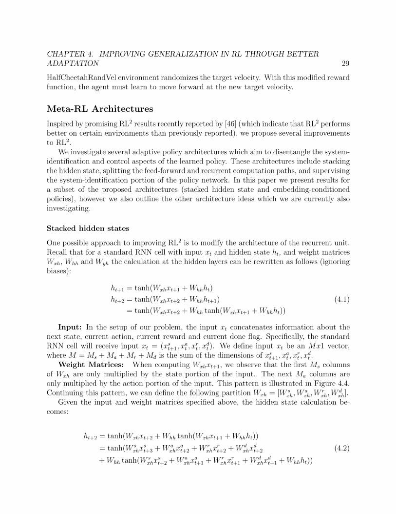
Input: In the setup of our problem, the input xt concatenates information about thenext state, current action, current reward and current done flag. Specifically, the standardRNN cell will receive input xt = (xs
t+1, xat , x
rt , x
dt ). We define input xt be an Mx1 vector,
where M = Ms +Ma +Mr +Md is the sum of the dimensions of xst+1, x
at , x
rt , x
dt .
Weight Matrices: When computing Wxhxt+1, we observe that the first Ms columnsof Wxh are only multiplied by the state portion of the input. The next Ma columns areonly multiplied by the action portion of the input. This pattern is illustrated in Figure 4.4.Continuing this pattern, we can define the following partition Wxh = [W s
xh,Waxh,W
rxh,W
dxh].
Given the input and weight matrices specified above, the hidden state calculation be-comes:
ht+2 = tanh(Wxhxt+2 +Whh tanh(Wxhxt+1 +Whhht))
= tanh(W sxhx
st+3 +W a
xhxat+2 +W r
xhxrt+2 +W d
xhxdt+2
+Whh tanh(Wsxhx
st+2 +W a
xhxat+1 +W r
xhxrt+1 +W d
xhxdt+1 +Whhht))
(4.2)
CHAPTER 4. IMPROVING GENERALIZATION IN RL THROUGH BETTERADAPTATION 30
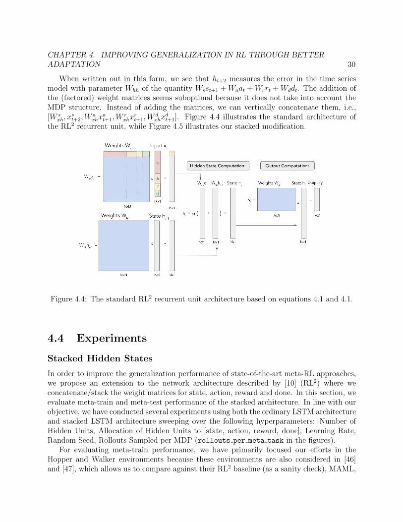
When written out in this form, we see that ht+2 measures the error in the time seriesmodel with parameter Whh of the quantity Wsst+1 +Waat +Wrrt +Wddt. The addition ofthe (factored) weight matrices seems suboptimal because it does not take into account theMDP structure. Instead of adding the matrices, we can vertically concatenate them, i.e.,[W s
xh, xst+2,W
axhx
at+1,W
rxhx
rt+1,W
dxhx
dt+1]. Figure 4.4 illustrates the standard architecture of
the RL2 recurrent unit, while Figure 4.5 illustrates our stacked modification.
Figure 4.4: The standard RL2 recurrent unit architecture based on equations 4.1 and 4.1.
4.4 Experiments
Stacked Hidden States
In order to improve the generalization performance of state-of-the-art meta-RL approaches,we propose an extension to the network architecture described by [10] (RL2) where weconcatenate/stack the weight matrices for state, action, reward and done. In this section, weevaluate meta-train and meta-test performance of the stacked architecture. In line with ourobjective, we have conducted several experiments using both the ordinary LSTM architectureand stacked LSTM architecture sweeping over the following hyperparameters: Number ofHidden Units, Allocation of Hidden Units to [state, action, reward, done], Learning Rate,Random Seed, Rollouts Sampled per MDP (rollouts per meta task in the figures).
For evaluating meta-train performance, we have primarily focused our e↵orts in theHopper and Walker environments because these environments are also considered in [46]and [47], which allows us to compare against their RL2 baseline (as a sanity check), MAML,
CHAPTER 4. IMPROVING GENERALIZATION IN RL THROUGH BETTERADAPTATION 31
Figure 4.5: Our proposed stacked RL2 recurrent unit architecture, which accounts for theMDP structure by disentangling the state, action, reward and done inputs.
as well as PEARL and ProMP. In these experiments, we focus on generalization with respectto environment dynamics (i.e., the RandParams environments), where each task/MDP is adi↵erent randomization of the simulation parameters, including friction, joint mass, andinertia.
Ordinary LSTM vs. Stacked LSTM
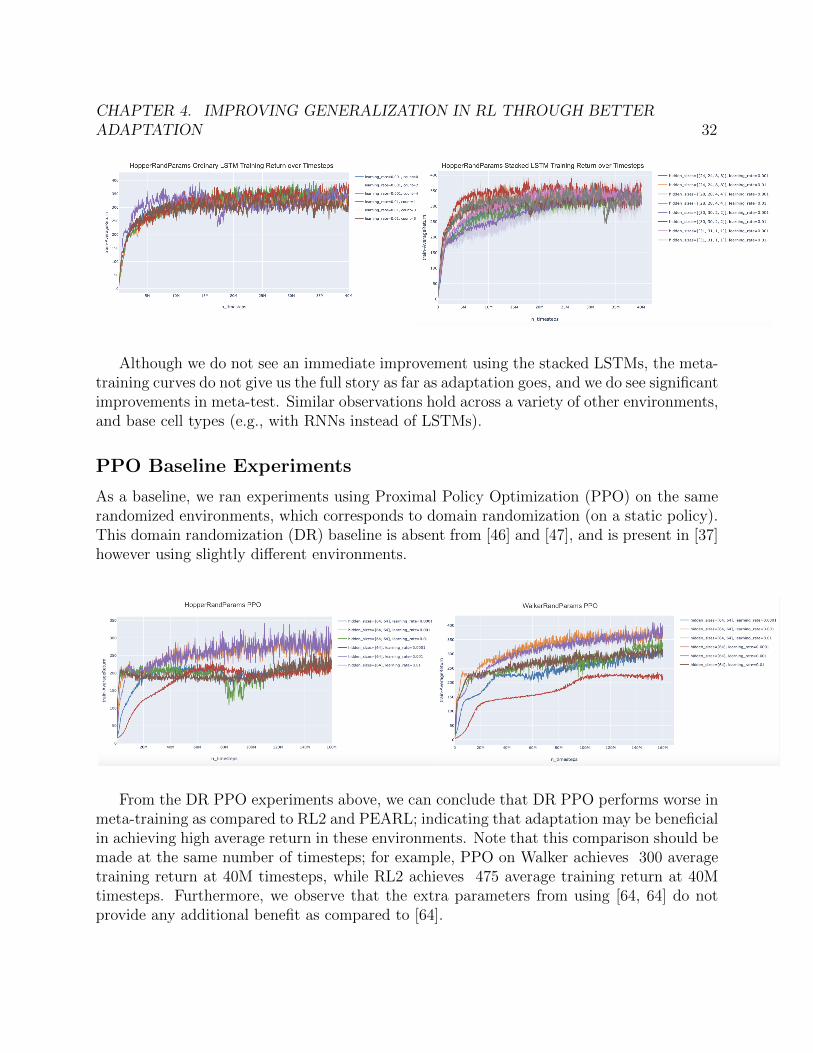
Our preliminary analysis focuses on comparing average return during training betweenstacked and unstacked LSTMs. We ran initial experiments on the Hopper environmentusing 64 hidden units and a variety of di↵erent learning rates. The figure below displaysthe average training return from using an ordinary LSTM (on left) and a stacked LSTM (onright).
CHAPTER 4. IMPROVING GENERALIZATION IN RL THROUGH BETTERADAPTATION 32
Although we do not see an immediate improvement using the stacked LSTMs, the meta-training curves do not give us the full story as far as adaptation goes, and we do see significantimprovements in meta-test. Similar observations hold across a variety of other environments,and base cell types (e.g., with RNNs instead of LSTMs).
PPO Baseline Experiments
As a baseline, we ran experiments using Proximal Policy Optimization (PPO) on the samerandomized environments, which corresponds to domain randomization (on a static policy).This domain randomization (DR) baseline is absent from [46] and [47], and is present in [37]however using slightly di↵erent environments.
From the DR PPO experiments above, we can conclude that DR PPO performs worse inmeta-training as compared to RL2 and PEARL; indicating that adaptation may be beneficialin achieving high average return in these environments. Note that this comparison should bemade at the same number of timesteps; for example, PPO on Walker achieves 300 averagetraining return at 40M timesteps, while RL2 achieves 475 average training return at 40Mtimesteps. Furthermore, we observe that the extra parameters from using [64, 64] do notprovide any additional benefit as compared to [64].
CHAPTER 4. IMPROVING GENERALIZATION IN RL THROUGH BETTERADAPTATION 33
Ablation Experiments
The policy architecture in the original RL2 paper takes in the [state, action, reward, done]inputs, however, no ablation is done over the set of inputs to determine if the network isreally utilizing the additional information. In our new stacked architecture, each of theseinputs is allocated a certain number of hidden units. We first run ablation experiments onthe stacked architecture, zeroing out each of the 4 inputs one at a time. These ablationexperiments help illustrate which inputs are important per environment, which may informhow to modify/improve the RL2 architecture.
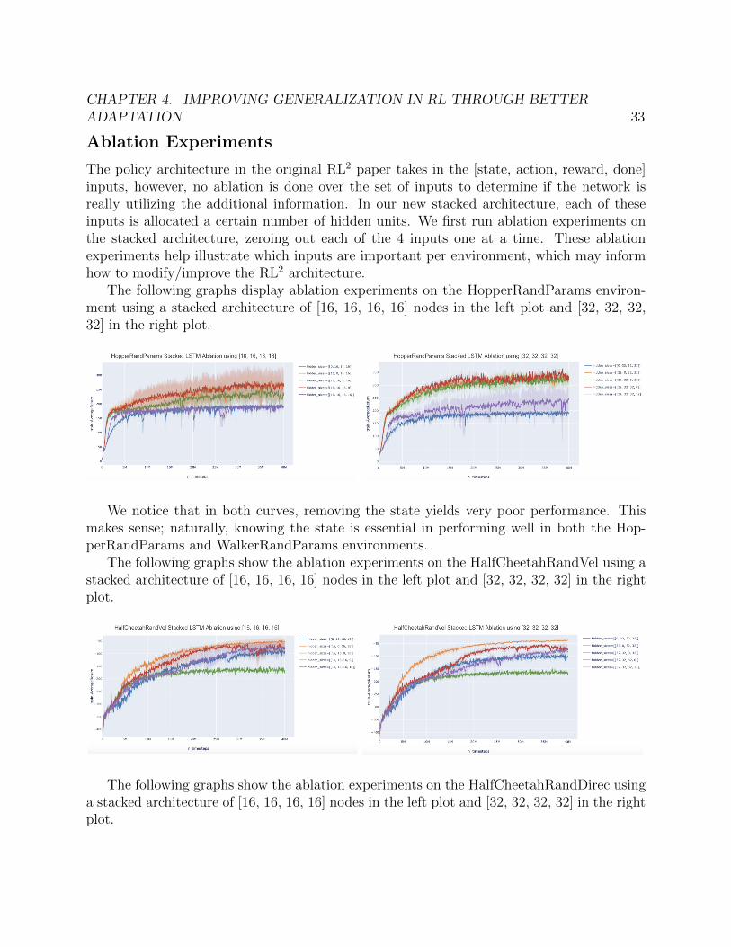
The following graphs display ablation experiments on the HopperRandParams environ-ment using a stacked architecture of [16, 16, 16, 16] nodes in the left plot and [32, 32, 32,32] in the right plot.
We notice that in both curves, removing the state yields very poor performance. Thismakes sense; naturally, knowing the state is essential in performing well in both the Hop-perRandParams and WalkerRandParams environments.
The following graphs show the ablation experiments on the HalfCheetahRandVel using astacked architecture of [16, 16, 16, 16] nodes in the left plot and [32, 32, 32, 32] in the rightplot.
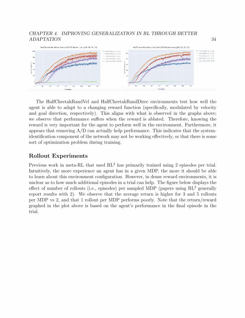
The following graphs show the ablation experiments on the HalfCheetahRandDirec usinga stacked architecture of [16, 16, 16, 16] nodes in the left plot and [32, 32, 32, 32] in the rightplot.
CHAPTER 4. IMPROVING GENERALIZATION IN RL THROUGH BETTERADAPTATION 34
The HalfCheetahRandVel and HalfCheetahRandDirec environments test how well theagent is able to adapt to a changing reward function (specifically, modulated by velocityand goal direction, respectively). This aligns with what is observed in the graphs above;we observe that performance su↵ers when the reward is ablated. Therefore, knowing thereward is very important for the agent to perform well in the environment. Furthermore, itappears that removing A/D can actually help performance. This indicates that the system-identification component of the network may not be working e↵ectively, or that there is somesort of optimization problem during training.
Rollout Experiments
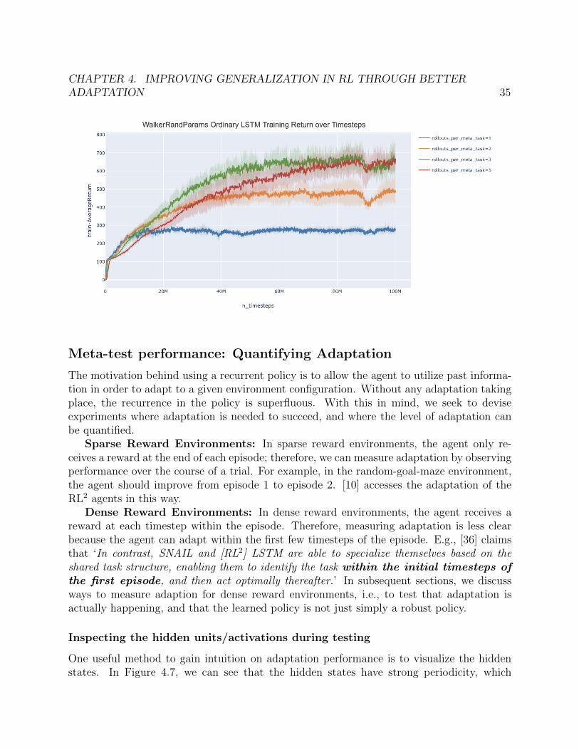
Previous work in meta-RL that used RL2 has primarily trained using 2 episodes per trial.Intuitively, the more experience an agent has in a given MDP, the more it should be ableto learn about this environment configuration. However, in dense reward environments, it isunclear as to how much additional episodes in a trial can help. The figure below displays thee↵ect of number of rollouts (i.e., episodes) per sampled MDP (papers using RL2 generallyreport results with 2). We observe that the average return is higher for 3 and 5 rolloutsper MDP vs 2, and that 1 rollout per MDP performs poorly. Note that the return/rewardgraphed in the plot above is based on the agent’s performance in the final episode in thetrial.
CHAPTER 4. IMPROVING GENERALIZATION IN RL THROUGH BETTERADAPTATION 35
Meta-test performance: Quantifying Adaptation
The motivation behind using a recurrent policy is to allow the agent to utilize past informa-tion in order to adapt to a given environment configuration. Without any adaptation takingplace, the recurrence in the policy is superfluous. With this in mind, we seek to deviseexperiments where adaptation is needed to succeed, and where the level of adaptation canbe quantified.
Sparse Reward Environments: In sparse reward environments, the agent only re-ceives a reward at the end of each episode; therefore, we can measure adaptation by observingperformance over the course of a trial. For example, in the random-goal-maze environment,the agent should improve from episode 1 to episode 2. [10] accesses the adaptation of theRL2 agents in this way.
Dense Reward Environments: In dense reward environments, the agent receives areward at each timestep within the episode. Therefore, measuring adaptation is less clearbecause the agent can adapt within the first few timesteps of the episode. E.g., [36] claimsthat ‘In contrast, SNAIL and [RL
2] LSTM are able to specialize themselves based on the
shared task structure, enabling them to identify the task within the initial timesteps ofthe first episode, and then act optimally thereafter.’ In subsequent sections, we discussways to measure adaption for dense reward environments, i.e., to test that adaptation isactually happening, and that the learned policy is not just simply a robust policy.
Inspecting the hidden units/activations during testing
One useful method to gain intuition on adaptation performance is to visualize the hiddenstates. In Figure 4.7, we can see that the hidden states have strong periodicity, which
CHAPTER 4. IMPROVING GENERALIZATION IN RL THROUGH BETTERADAPTATION 36
upon further inspection (aligning the x-axis to the timesteps in Mujoco renderings) we cansee correspond to the periodicity in the Hopper’s movement (see Figure 4.6). Howeverthese visualizations alone are not indicative that the hidden state is being used to learn anenvironment embedding for system identification.
In order to better understand/visualize the patterns within the hidden states, we canadditionally perform Principal Component Analysis (PCA) and project the high dimensionalstates onto a 2D plane. In the simple case where we vary only one free variable (eg friction),if we sample E trajectories from T trials/MDPs, we should expect the activations alongeach trajectory from the same trial/MDP to be in a cluster. For example, the hidden stateactivations for trajectories in high friction environments should be clustered together, whilelow friction trajectories should be in a separate cluster. We are currently implementingcluster visualizations for hidden states at test-time, and will include them in a subsequentiteration of this research paper. Additionally, we are investigating inspecting the gradientsduring meta-training to better understand what the hidden state is learning.
Continual Adaptation Experiments
In a dense reward environment, the recurrent policy should ostensibly adapt within the firstfew timesteps of an episode, unlike in a sparse reward environment, where adaptation willoccur on the scale of episodes (instead of timesteps). Because adaptation happens within anepisode in dense reward environments (e.g., Mujoco locomotion envs), it is hard to discernbetween an adaptive policy and a robust policy. One way to tell the di↵erence is to deploythe agent in an environment where it needs to continually adapt to changing goals or dynam-ics. In the subsequent sections, we test the adaptive policies on HalfCheetahRandDirec andRandVel environments where the goal direction and goal/target velocity change mid-episode.For the target velocity envs, we test both interpolation (target velocities within the original[0,3] range), and extrapolation to a new target velocity (4).
For RandVel, we test on three scenarios:
1. Interpolation: Goal velocity sequence of [0,1,2,3] at 50 timestep intervals
2. Extrapolation 1: Goal velocity sequence of [1,2,3,4] at 50 timestep intervals
3. Extrapolation 2: Goal velocity sequence of [3,4] at 100 timestep intervals
For RandDirec, we test on two scenarios:
1. Backwards-Forwards: Target direction switches from Backwards to Forwards mid-episode (100 timesteps)
2. Forwards-Backwards: Opposite of Backwards-Forwards
In the subsequent sections, we provide high-level conclusions from our results for brevity,but include the full suite of experiments in Section ?? and Section 4.4.
CHAPTER 4. IMPROVING GENERALIZATION IN RL THROUGH BETTERADAPTATION 37
Does RL2 continually adapt on HalfCheetahRandVel?
We perform experiments to evaluate how well RL2 adapts on the HalfCheetahRandVel en-vironment. If the agent is adapting perfectly, the graph should look like a sawtooth wave,where the cheetah slows down / speeds up until it hits goal velocity, then cruises at the goalvelocity.
We performed continual adaptation experiments using both an Ordinary RNN and StackedRNN with 64 units. Interpolation and Extrapolation results are shown in Figure 4.8, Figure4.9 and Figure 4.10. We can draw the following conclusions:
BasicRNNStackInputs (64 units) vs BasicRNN (64 units)
1. Interpolation: The stacked architecture is marginally better. Based on the rewardtrajectories, the stacked architecture is able to adapt to final goal velocity better.
2. Extrapolation 1 and 2: The stacked architecture is much better, and actually has thebest (highest) terminal goal velocity.
Does RL2 continually adapt on HalfCheetahRandDirec?
In order to measure how RL2 continually adapts in the HalfCheetahRandDirec environment,we change the direction midway through the episode and analyze how well the agent is ableto adapt to this new reward function. We test on both scenarios: changing backwards toforwards and changing forwards to backwards.
We performed continual adaptation experiments using both an Ordinary RNN and StackedRNN with 64 units. Forward-to-Backward and Backward-to-Forward results are shown inFigure 4.11 and Figure 4.12. We can draw the following conclusions:
BasicRNNStackInputs (64 units) vs BasicRNN (64 units)
1. Back to Forward: Based on the cumulative reward and overall reward trajectories, thestacked architecture performs much better.
2. Forward to Back: Based on the cumulative reward and overall reward trajectories, thestacked architecture performs much better.
Takeaway: In both cases, we can see that the stacked architecture is quite promising,indicating that the stacked hidden states architecture can enable significantly better adap-tation to new, changing environments. Additionally, it seems that the stacked architecturehas the best extrapolation performance. We are planning on expanding the number of testenvironments to include environments with continually changing dynamics (in addition tochanging goals) to further investigate these results and see if they still hold.
CHAPTER 4. IMPROVING GENERALIZATION IN RL THROUGH BETTERADAPTATION 38
4.5 Conclusion and Future Work
Our preliminary analysis indicates that the stacked hidden states architecture can enable sig-nificantly better adaptation to new, changing environments. We are planning on expandingthe number of test environments to include environments with continually changing dynam-ics (in addition to changing goals) to further investigate these results and see if they stillhold.
Another direction is to investigate test-time adaptation to environments with sparserewards, such as mazes with varying goals (a common benchmark in prior work) to see ifour preliminary observations still hold, as well as evaluating our new architectures on therecently released Meta-World benchmark. [63].
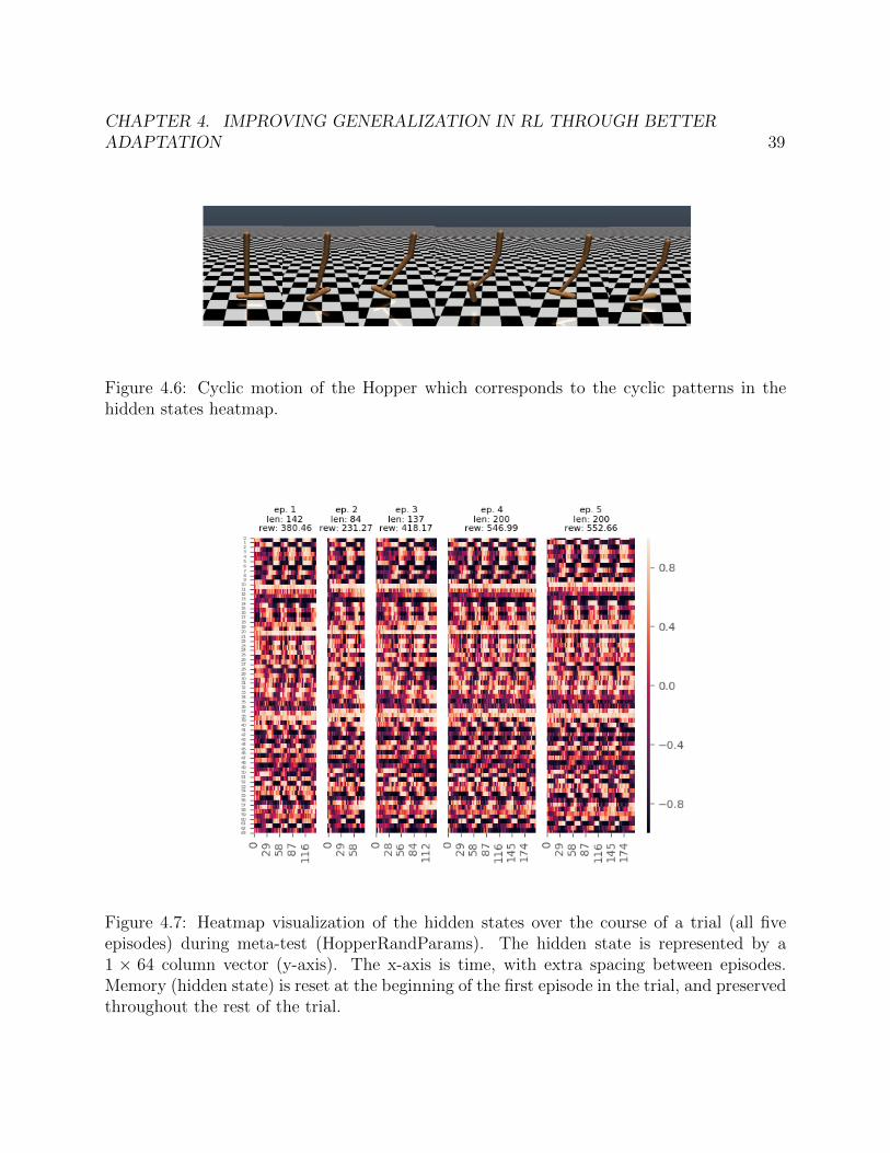
CHAPTER 4. IMPROVING GENERALIZATION IN RL THROUGH BETTERADAPTATION 39
Figure 4.6: Cyclic motion of the Hopper which corresponds to the cyclic patterns in thehidden states heatmap.
Figure 4.7: Heatmap visualization of the hidden states over the course of a trial (all fiveepisodes) during meta-test (HopperRandParams). The hidden state is represented by a1 ⇥ 64 column vector (y-axis). The x-axis is time, with extra spacing between episodes.Memory (hidden state) is reset at the beginning of the first episode in the trial, and preservedthroughout the rest of the trial.
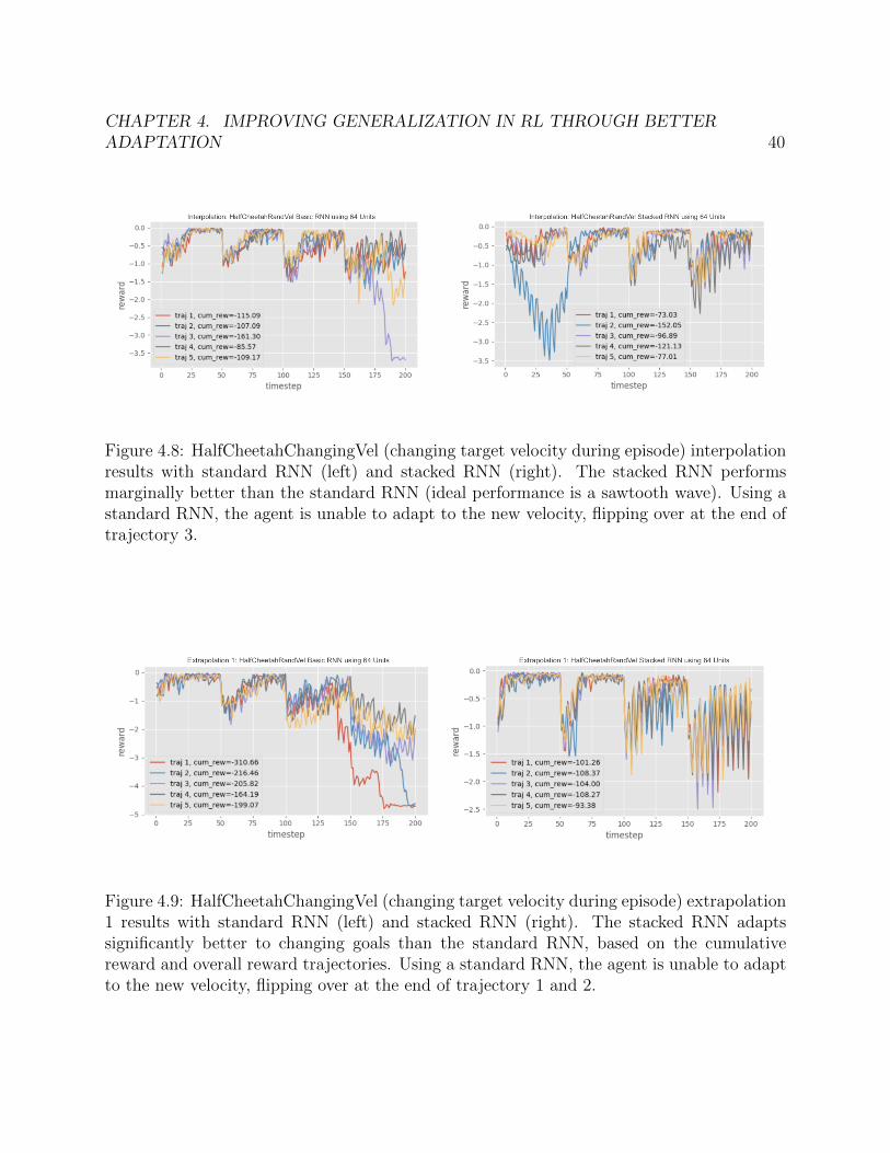
CHAPTER 4. IMPROVING GENERALIZATION IN RL THROUGH BETTERADAPTATION 40
Figure 4.8: HalfCheetahChangingVel (changing target velocity during episode) interpolationresults with standard RNN (left) and stacked RNN (right). The stacked RNN performsmarginally better than the standard RNN (ideal performance is a sawtooth wave). Using astandard RNN, the agent is unable to adapt to the new velocity, flipping over at the end oftrajectory 3.
Figure 4.9: HalfCheetahChangingVel (changing target velocity during episode) extrapolation1 results with standard RNN (left) and stacked RNN (right). The stacked RNN adaptssignificantly better to changing goals than the standard RNN, based on the cumulativereward and overall reward trajectories. Using a standard RNN, the agent is unable to adaptto the new velocity, flipping over at the end of trajectory 1 and 2.
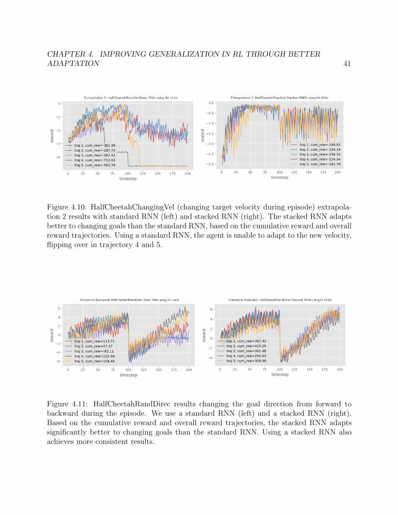
CHAPTER 4. IMPROVING GENERALIZATION IN RL THROUGH BETTERADAPTATION 41
Figure 4.10: HalfCheetahChangingVel (changing target velocity during episode) extrapola-tion 2 results with standard RNN (left) and stacked RNN (right). The stacked RNN adaptsbetter to changing goals than the standard RNN, based on the cumulative reward and overallreward trajectories. Using a standard RNN, the agent is unable to adapt to the new velocity,flipping over in trajectory 4 and 5.
Figure 4.11: HalfCheetahRandDirec results changing the goal direction from forward tobackward during the episode. We use a standard RNN (left) and a stacked RNN (right).Based on the cumulative reward and overall reward trajectories, the stacked RNN adaptssignificantly better to changing goals than the standard RNN. Using a stacked RNN alsoachieves more consistent results.
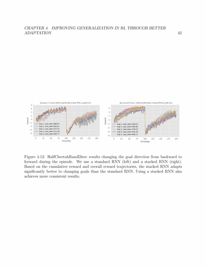
CHAPTER 4. IMPROVING GENERALIZATION IN RL THROUGH BETTERADAPTATION 42
Figure 4.12: HalfCheetahRandDirec results changing the goal direction from backward toforward during the episode. We use a standard RNN (left) and a stacked RNN (right).Based on the cumulative reward and overall reward trajectories, the stacked RNN adaptssignificantly better to changing goals than the standard RNN. Using a stacked RNN alsoachieves more consistent results.
43
Chapter 5
Conclusion and Future Work
In this work, we proposed and evaluated solutions to salient transfer learning problems inboth Natural Language Processing and Reinforcement Learning.
In Chapter 3, we presented a test-time training technique that leverages unsupervisedinformation from the test example and similar training examples to adapt NLP models.Further work should focus on how training with MLM loss during fine-tuning changes bothin-distribution and out-of-distribution performance. A possible other direction is to studythe e↵ect of fine-tuning on the MLM loss of in-domain and OOD examples. This would helpunderstand what fine-tuning is exactly doing to the embeddings.
In Chapter 4, we proposed and evaluated a meta-RL architectures based on the archi-tecture and training algorithm described by previous work (ie. RL2) [10]. Our architecturalchanges improves adaptation to new environments by disentangling the recurrent and feedforward components of the recurrent policy network. One direction to investigate is test-time adaptation to environments with sparse rewards, such as mazes with varying goals (acommon benchmark in prior work) to see if our preliminary observations still hold, as wellas evaluating our new architectures on the recently released Meta-World benchmark.
44
Bibliography
[1] Iz Beltagy, Arman Cohan, and Kyle Lo. “Scibert: Pretrained contextualized embed-dings for scientific text”. In: arXiv preprint arXiv:1903.10676 (2019).
[2] Dallas Card, Michael Zhang, and Noah A. Smith. “Deep Weighted Averaging Classi-fiers”. In: FAT. 2018.
[3] Daniel Cer et al. “SemEval-2017 Task 1: Semantic textual similarity-multilingual andcross-lingual focused evaluation”. In: SemEval. 2017.
[4] Ignasi Clavera et al. “Learning to Adapt: Meta-Learning for Model-Based Control”.In: arXiv:1803.11347 (2018).
[5] Gabriela Csurka. “Domain adaptation for visual applications: A comprehensive sur-vey”. In: arXiv preprint arXiv:1702.05374 (2017).
[6] Andrew M Dai and Quoc V Le. “Semi-supervised sequence learning”. In: 2015.
[7] Jacob Devlin et al. “BERT: Pre-training of Deep Bidirectional Transformers for Lan-guage Understanding”. In: NAACL-HLT. 2019.
[8] Yunshu Du et al. “Adapting auxiliary losses using gradient similarity”. In: arXiv
preprint arXiv:1812.02224 (2018).
[9] Yan Duan et al. “Benchmarking deep reinforcement learning for continuous control”.In: International Conference on Machine Learning. 2016, pp. 1329–1338.
[10] Yan Duan et al. “RL2: Fast Reinforcement Learning via Slow Reinforcement Learning”.In: arXiv:1611.02779 (2016).
[11] Chelsea Finn, Pieter Abbeel, and Sergey Levine. “Model-Agnostic Meta-Learning forFast Adaptation of Deep Networks”. In: 2017.
[12] Chelsea Finn, Pieter Abbeel, and Sergey Levine. “Model-agnostic meta-learning forfast adaptation of deep networks”. In: ICML. 2017.
[13] Yaroslav Ganin et al. “Domain-adversarial training of neural networks”. In: The Jour-
nal of Machine Learning Research. 2016.
[14] Xavier Glorot, Antoine Bordes, and Yoshua Bengio. “Domain adaptation for large-scalesentiment classification: A deep learning approach”. In: 2011.
BIBLIOGRAPHY 45
[15] Xiaoxiao Guo et al. “Deep learning for real-time Atari game play using o✏ine Monte-Carlo tree search planning”. In: Advances in neural information processing systems.2014, pp. 3338–3346.
[16] Suchin Gururangan et al. “Don’t Stop Pretraining: Adapt Language Models to Do-mains and Tasks”. In: 2020.
[17] Xiaochuang Han and Jacob Eisenstein. “Unsupervised domain adaptation of contex-tualized embeddings: A case study in early modern english”. In: EMNLP. 2019.
[18] Ruining He and Julian J. McAuley. “Ups and Downs: Modeling the Visual Evolutionof Fashion Trends with One-Class Collaborative Filtering”. In: WWW. 2016.
[19] Dan Hendrycks and Thomas Dietterich. “Benchmarking Neural Network Robustnessto Common Corruptions and Perturbations”. In: ICLR. 2019.
[20] Dan Hendrycks, Kimin Lee, and Mantas Mazeika. “Using pre-training can improvemodel robustness and uncertainty”. In: 2019.
[21] Dan Hendrycks et al. “Pretrained Transformers Improve Out-of-Distribution Robust-ness”. In: 2020.
[22] Dan Hendrycks et al. “Using self-supervised learning can improve model robustnessand uncertainty”. In: NeurIPS. 2019.
[23] Jeremy Howard and Sebastian Ruder. “Universal language model fine-tuning for textclassification”. In: 2018.
[24] Kexin Huang, Jaan Altosaar, and Rajesh Ranganath. “Clinicalbert: Modeling clini-cal notes and predicting hospital readmission”. In: arXiv preprint arXiv:1904.05342
(2019).
[25] Max Jaderberg et al. “Reinforcement learning with unsupervised auxiliary tasks”. In:2017.
[26] Anthony Kroch, Beatrice Santorini, and Ariel Diertani. “Penn-Helsinki Parsed Corpusof Early Modern English”. In: (2004). url: http://www.ling.upenn.edu/hist-corpora/PPCEME-RELEASE-2/index.html.
[27] Keita Kurita, Paul Michel, and Graham Neubig. “Weight Poisoning Attacks on Pre-trained Models”. In: ACL. 2020.
[28] Jinhyuk Lee et al. “BioBERT: a pre-trained biomedical language representation modelfor biomedical text mining”. In: Bioinformatics 36.4 (2020), pp. 1234–1240.
[29] Sergey Levine et al. “End-to-end training of deep visuomotor policies”. In: The Journalof Machine Learning Research 17.1 (2016), pp. 1334–1373.
[30] Andrew L Maas et al. “Learning word vectors for sentiment analysis”. In: ACL. 2011.
[31] Aleksander Madry et al. “Towards deep learning models resistant to adversarial at-tacks”. In: 2018.
BIBLIOGRAPHY 46
[32] Mitchell P. Marcus, Mary Ann Marcinkiewicz, and Beatrice Santorini. “Building alarge annotated corpus of English: The Penn Treebank”. In: Computational Linguistics.1993.
[33] Julian J. McAuley et al. “Image-based Recommendations on Styles and Substitutes”.In: SIGIR. 2015.
[34] Michael McCloskey and Neal J Cohen. “Catastrophic Interference in ConnectionistNetworks: The Sequential Learning Problem”. In: Psychology of learning and motiva-
tion. 1989.
[35] Piotr Mirowski et al. “Learning to navigate in complex environments”. In: 2017.
[36] Nikhil Mishra et al. “A Simple Neural Attentive Meta-Learner”. In: 2018.
[37] Charles Packer et al. “Assessing Generalization in Deep Reinforcement Learning”. In:arXiv:1810.12282 (2019).
[38] Sinno Jialin Pan and Qiang Yang. “A survey on transfer learning”. In: IEEE TKDE.2009.
[39] Georgios Papoudakis, Kyriakos C. Chatzidimitriou, and Pericles A. Mitkas. “Deepreinforcement learning for doom using unsupervised auxiliary tasks”. In: arXiv preprintarXiv:1807.01960 (2018).
[40] Adam Paszke et al. “PyTorch: An imperative style, high-performance deep learninglibrary”. In: 2019.
[41] Giorgio Patrini et al. “Making deep neural networks robust to label noise: A losscorrection approach”. In: 2017.
[42] Matthew E. Peters et al. “Deep contextualized word representations”. In: 2018.
[43] Lerrel Pinto et al. “Robust Adversarial Reinforcement Learning”. In: 2017.
[44] Evani Radiya-Dixit and Xin Wang. “How fine can fine-tuning be? Learning e�cientlanguage models”. In: arXiv preprint arXiv:2004.14129 (2020).
[45] Aravind Rajeswaran et al. “EPOpt: Learning robust neural network policies usingmodel ensembles”. In: 2017.
[46] Kate Rakelly et al. “E�cient O↵-Policy Meta-Reinforcement learning via ProbabilisticContext Variables”. In: 2019.
[47] Jonas Rothfuss et al. “ProMP: Proximal Meta-Policy Search”. In: 2019.
[48] Sebastian Ruder. “Neural Transfer Learning for Natural Language Processing”. PhDthesis. National University of Ireland, Galway, 2019.
[49] Steindor Sæmundsson, Katja Hofmann, and Marc Peter Deisenroth. “Meta Reinforce-ment Learning with Latent Variable Gaussian Processes”. In: 2018.
[50] Erik F Sang and Fien De Meulder. “Introduction to the CoNLL-2003 shared task:Language-independent named entity recognition”. In: arXiv preprint cs/0306050 (2003).
BIBLIOGRAPHY 47
[51] John Schulman et al. “High-dimensional continuous control using generalized advan-tage estimation”. In: arXiv preprint arXiv:1506.02438 (2015).
[52] Darsh J Shah et al. “Adversarial domain adaptation for duplicate question detection”.In: 2018.
[53] Jian Shen et al. “Wasserstein distance guided representation learning for domain adap-tation”. In: 2018.
[54] Richard Socher et al. “Recursive deep models for semantic compositionality over asentiment treebank”. In: EMNLP. 2013.
[55] Benjamin Strauss et al. “Results of the wnut16 named entity recognition shared task”.In: Proceedings of the 2nd Workshop on Noisy User-generated Text (WNUT). 2016,pp. 138–144.
[56] Yu Sun et al. “Test-time training for out-of-distribution generalization”. In: arXivpreprint arXiv:1909.13231 (2019).
[57] Yu Sun et al. “Unsupervised Domain Adaptation through Self-Supervision”. In: arXivpreprint arXiv:1909.11825 (2019).
[58] Flood Sung et al. “Learning to learn: Meta-critic networks for sample e�cient learn-ing”. In: arXiv:1706.09529 (2017).
[59] Eric Tzeng et al. “Adversarial discriminative domain adaptation”. In: 2017.
[60] Alex Wang et al. “Glue: A multi-task benchmark and analysis platform for naturallanguage understanding”. In: arXiv preprint arXiv:1804.07461 (2018).
[61] Jane X Wang et al. “Learning to reinforcement learn”. In: arXiv:1611.05763 (2016).
[62] Thomas Wolf et al. “Transformers: State-of-the-art Natural Language Processing”. In:arXiv preprint arXiv:1910.03771 (2019).
[63] Tianhe Yu et al. “Meta-world: A benchmark and evaluation for multi-task and metareinforcement learning”. In: arXiv preprint arXiv:1910.10897 (2019).
[64] Yuting Zhang, Kibok Lee, and Honglak Lee. “Augmenting supervised neural networkswith unsupervised objectives for large-scale image classification”. In: 2016.
[65] Yukun Zhu et al. “Aligning books and movies: Towards story-like visual explanationsby watching movies and reading books”. In: Proceedings of the IEEE international
conference on computer vision. 2015, pp. 19–27.