Embed Size (px)
Citation preview
A Study on Expectiles:
Measuring Risk in Finance
by
Andrew Lewis Anderson
(Under the Direction of Cheolwoo Park)
Abstract
In this thesis, we examine the properties that make the expectile a proper candidate for a
measure of risk in finance. Expectiles are the solutions to asymmetric least squares mini-
mization. The expectile is also closely related to two commonly used measures, value at risk
and expected shortfall, which facilitates the extension of the expectile to finance. Using sim-
ulated examples, we investigate characteristics that make the expectile attractive in finance.
The relationship between quantiles and expectiles is featured prominently. In addition, a
method for estimating the time-varying expectile is outlined and applied to an exchange
traded fund of the Dow Jones Industrial Average and the S&P 500 Stock Index.
Index words: expectiles, quantiles, risk measures, coherence, value at risk, GARCH,Normal Inverse Gaussian distribution, asymmetric least squares
A Study on Expectiles:
Measuring Risk in Finance
by
Andrew Lewis Anderson
B.S., Armstrong Atlantic State University, 2010
A Dissertation Submitted to the Graduate Faculty
of The University of Georgia in Partial Fulfillment
of the
Requirements for the Degree
Master of Science
Athens, Georgia
2012

c©2012
Andrew Lewis Anderson
A Study on Expectiles:
Measuring Risk in Finance
by
Andrew Lewis Anderson
Approved:
Major Professor: Cheolwoo Park
Committee: Lynne SeymourLily Wang
Electronic Version Approved:
Maureen GrassoDean of the Graduate SchoolThe University of GeorgiaDecember 2012
A Study on Expectiles:
Measuring Risk in Finance
Andrew Lewis Anderson
October 26, 2012
Acknowledgments
I would like to thank my wife and my major professor for their guidance and support, but
most of all for their patience.
1
Contents
List of Figures 4
List of Tables 6
1 Introduction 7
2 Literature Review 9
2.1 Financial Time Series . . . . . . . . . . . . . . . . . . . . . . . . . . . . . . . 9
2.2 Risk Measures . . . . . . . . . . . . . . . . . . . . . . . . . . . . . . . . . . . 11
3 Expectiles 16
3.1 Properties . . . . . . . . . . . . . . . . . . . . . . . . . . . . . . . . . . . . . 16
3.2 Interpretation . . . . . . . . . . . . . . . . . . . . . . . . . . . . . . . . . . . 19
3.3 Time-Varying Expectiles . . . . . . . . . . . . . . . . . . . . . . . . . . . . . 20
4 Numerical Analysis 24
4.1 Simulation . . . . . . . . . . . . . . . . . . . . . . . . . . . . . . . . . . . . . 24
4.2 Real Data . . . . . . . . . . . . . . . . . . . . . . . . . . . . . . . . . . . . . 28
5 Conclusions and Future Work 31
A Additional Results for DJIA analysis 33
B Results for S&P 500 38
C Backtesting Test Statistic 44
2

D Bibliography 46
3
List of Figures
2.1 The top graph is a time series of the raw MSFT stock price, while bottom
graph is a graph of the log returns over the same period. . . . . . . . . . . . 10
2.2 5% Value at Risk (labeled VaR) and corresponding Expected Shortfall (labeled
TVaR) for a skewed distribution. . . . . . . . . . . . . . . . . . . . . . . . . 15
3.1 NIG distributions with different parameters . . . . . . . . . . . . . . . . . . 22
4.1 Simulations generated using εt ∼ NIG(0, 1, 0, 1). . . . . . . . . . . . . . . . . 25
4.2 Simulations generated using εt ∼ N(0, 1). . . . . . . . . . . . . . . . . . . . . 26
4.3 Simulations generated using εt ∼ t(df = 5). . . . . . . . . . . . . . . . . . . . 26
4.4 Sample quantiles vs. sample expectiles for corresponding values of τ and α . 27
4.5 Time-varying Expectile for Dow Jones . . . . . . . . . . . . . . . . . . . . . 29
A.1 ACF of Squared Returns and Squared Residuals . . . . . . . . . . . . . . . . 34
A.2 Log Returns, Fitted GARCH values, and GARCH residuals for Dow Jones data 35
A.3 Histogram of GARCH residuals. . . . . . . . . . . . . . . . . . . . . . . . . . 35
A.4 NIG QQ-plot to assess NIG fit . . . . . . . . . . . . . . . . . . . . . . . . . . 36
A.5 NIG fit of Residuals . . . . . . . . . . . . . . . . . . . . . . . . . . . . . . . . 37
B.1 Time Series of S&P Closing Prices, 01-02-2008 to 01-13-2012 . . . . . . . . . 38
B.2 ACF plots of log returns and squared log returns . . . . . . . . . . . . . . . 39
B.3 Histogram of GARCH residuals . . . . . . . . . . . . . . . . . . . . . . . . . 40
B.4 NIG QQ-plot of errors . . . . . . . . . . . . . . . . . . . . . . . . . . . . . . 41
B.5 Log Returns, Fitted GARCH values, and GARCH residuals for S&P data . . 41
4

B.6 NIG fit for S&P time series . . . . . . . . . . . . . . . . . . . . . . . . . . . 42
B.7 Time-varying Expectile for S&P . . . . . . . . . . . . . . . . . . . . . . . . . 43
5
List of Tables
3.1 τ and corresponding α for several distributions. . . . . . . . . . . . . . . . . 20
4.1 Backtesting Summary for DJIA ETF series VaR . . . . . . . . . . . . . . . . 30
B.1 Backtesting Summary for S&P 500 series VaR . . . . . . . . . . . . . . . . . 43
6
Chapter 1
Introduction
Practitioners have long used statistics to augment decision-making within the field of finance.
Analyses of portfolios and financial time series have become highly technical and increasingly
important for investment banks and other financial institutions. Specifically, models that
assess the risk of a financial asset or a portfolio have become the foundation for current
government regulations and allocation decisions within financial firms. Understanding the
innate risk of a financial position is essential for a firm balancing the capacity for losses with
the possibility of profits.
Risk is defined as the potential for an undesirable outcome (i.e. loss of value) resulting
from an action or inaction. In finance, risk is the uncertainty surrounding the future value
of an asset or portfolio of financial instruments. Measuring risk is essential to maintaining
a healthy and efficient financial system. Risk measures serve to rank financial instruments
and positions by the inherent risk, which encourages more efficient allocation of capital in
financial markets. In a regulatory framework, risk measures are used to establish capital
requirements. A good risk measure will balance the potential for catastrophic losses with
the potential for more efficient allocation of investment capital.
Current risk measures, while still popular, have serious shortcomings. The expectile, the
solution to asymmetric least squares regression, resolves many of the issues of previous risk
measures. In addition to addressing the shortcomings of other risk measures such as Value-
at-Risk and Expected Shortfall, expectiles have unique characteristics that make them very
7

efficient and informative measures of risk.
Our purpose here is to develop a time-varying expectile that measures the inherent risk of
an asset over time. Before introducing a parametric method for estimating the time-varying
expectile, risk measures and expectiles are expounded upon in the following chapters. The
method for constructing a time-varying expectile is then explained, followed by simulations
and real data analyses. Conclusions and future work complete the thesis.
8
Chapter 2
Literature Review
Chapter 2 discusses the background necessary to understand the application of expectiles to
finance. The first section of this chapter defines the context in which we are modeling, as
well as some of the subtleties of financial data. Risk measures are defined and elaborated on
in the next section.
2.1 Financial Time Series
Estimating the risk of a financial asset or position involves utilizing the information from
financial time series. A financial time series, in its raw form, is a series of asset values over
time. However, financial managers are more interested in the returns on an investment or
the changes in price of an asset over time.
If St is the price of a financial asset at time t, then the raw return rt from time t−∆t to
time t is St−St−∆t. This is the first difference of the series of stock prices, St. Instead of the
raw difference, St − St−∆t, we examine the time series of the differences of the log returns
rt = ln(St)− ln(St−∆t).
The series of differenced log returns will be referred to simply as the log returns and
denoted rt. The time period ∆t is generally taken to be 1. The use of log returns is standard
in finance due to their inherent mathematical tractability. Taking the differenced log returns
9
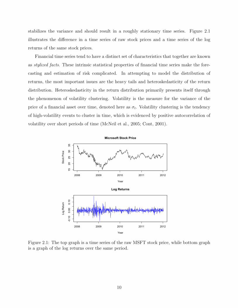
stabilizes the variance and should result in a roughly stationary time series. Figure 2.1
illustrates the difference in a time series of raw stock prices and a time series of the log
returns of the same stock prices.
Financial time series tend to have a distinct set of characteristics that together are known
as stylized facts. These intrinsic statistical properties of financial time series make the fore-
casting and estimation of risk complicated. In attempting to model the distribution of
returns, the most important issues are the heavy tails and heteroskedasticity of the return
distribution. Heteroskedasticity in the return distribution primarily presents itself through
the phenomenon of volatility clustering. Volatility is the measure for the variance of the
price of a financial asset over time, denoted here as σt. Volatility clustering is the tendency
of high-volatility events to cluster in time, which is evidenced by positive autocorrelation of
volatility over short periods of time (McNeil et al., 2005; Cont, 2001).
2008 2009 2010 2011 2012
1520
2530
35
Year
Sto
ck P
rice
Microsoft Stock Price
2008 2009 2010 2011 2012
-0.10
0.00
0.10
Year
Log
Ret
urn
Log Returns
Figure 2.1: The top graph is a time series of the raw MSFT stock price, while bottom graphis a graph of the log returns over the same period.
10
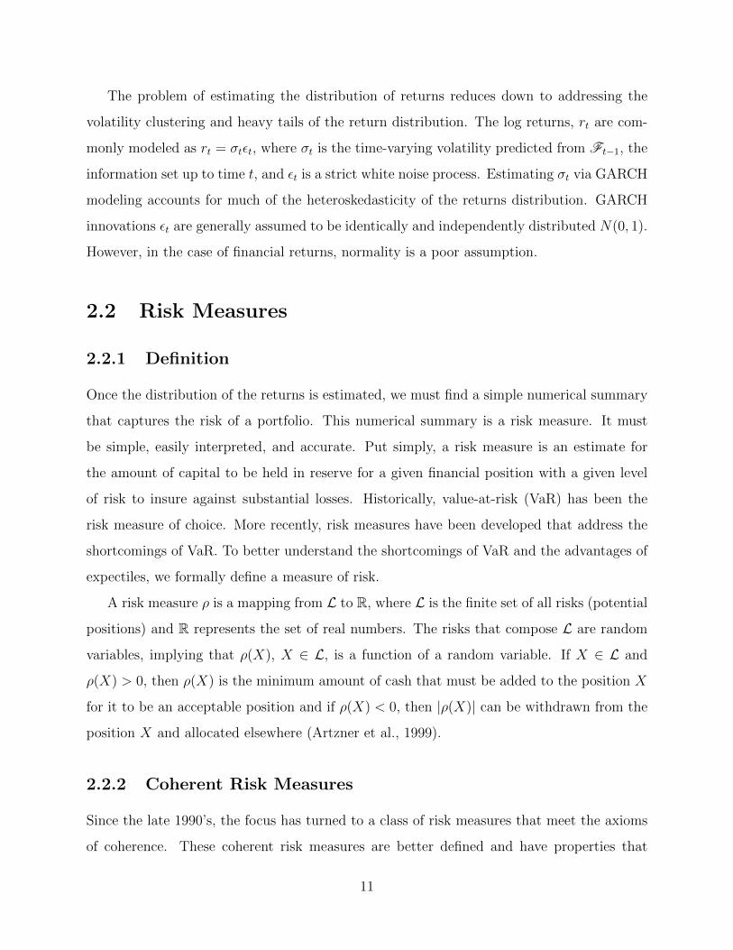
The problem of estimating the distribution of returns reduces down to addressing the
volatility clustering and heavy tails of the return distribution. The log returns, rt are com-
monly modeled as rt = σtεt, where σt is the time-varying volatility predicted from Ft−1, the
information set up to time t, and εt is a strict white noise process. Estimating σt via GARCH
modeling accounts for much of the heteroskedasticity of the returns distribution. GARCH
innovations εt are generally assumed to be identically and independently distributed N(0, 1).
However, in the case of financial returns, normality is a poor assumption.
2.2 Risk Measures
2.2.1 Definition
Once the distribution of the returns is estimated, we must find a simple numerical summary
that captures the risk of a portfolio. This numerical summary is a risk measure. It must
be simple, easily interpreted, and accurate. Put simply, a risk measure is an estimate for
the amount of capital to be held in reserve for a given financial position with a given level
of risk to insure against substantial losses. Historically, value-at-risk (VaR) has been the
risk measure of choice. More recently, risk measures have been developed that address the
shortcomings of VaR. To better understand the shortcomings of VaR and the advantages of
expectiles, we formally define a measure of risk.
A risk measure ρ is a mapping from L to R, where L is the finite set of all risks (potential
positions) and R represents the set of real numbers. The risks that compose L are random
variables, implying that ρ(X), X ∈ L, is a function of a random variable. If X ∈ L and
ρ(X) > 0, then ρ(X) is the minimum amount of cash that must be added to the position X
for it to be an acceptable position and if ρ(X) < 0, then |ρ(X)| can be withdrawn from the
position X and allocated elsewhere (Artzner et al., 1999).
2.2.2 Coherent Risk Measures
Since the late 1990’s, the focus has turned to a class of risk measures that meet the axioms
of coherence. These coherent risk measures are better defined and have properties that
11
satisfy modern theories of finance and investor expectations. There are four axioms that
a risk measure must satisfy to be coherent: translation invariance, monotonicity, positive
homogeneity, and sub-additivity. The four axioms are stated below using the previously
established notation.
Translation Invariance: For all X ∈ L and a ∈ R, ρ(X + a) = ρ(X)− a.
Translation invariance reinforces the intuitive notion that if cash is added to a position
(think of a portfolio), then the position now has less risk since the cash acts as insurance
against a loss in the original position. This axiom specifies that the actual risk will drop by
the amount of cash added to the portfolio.
Monotonicity: If X1, X2 ∈ L and X1 ≤ X2, then ρ(X2) ≤ ρ(X1) for all X1, X2.
If a portfolio X2 always has better values than portfolio X1, then X2 should be less risky
than X1.
Positive Homogeneity: For all a ≥ 0 and X ∈ L, ρ(aX) = aρ(X).
This reflects the idea that position size directly influences risk. If we double the size of
our position, we are exposed to double the amount of risk.
Sub-additivity: If X1, X2 ∈ L, then ρ(X1 +X2) ≤ ρ(X1) + ρ(X2).
The axiom of sub-additivity reflects the principle of diversification: the risk of the port-
folio should be less than the sum of the risks of the constituent parts.
While these axioms of coherence are just conventions, they establish a framework for
developing risk measures that capture essential properties of financial markets. Lack of
coherence does not preclude a risk measure from being used. We can use the the concept
of coherence to identify the limitations of a risk measure and to improve it. The following
section discusses two of the more popular risk measures used in finance, Value-at-Risk and
Expected Shortfall.
2.2.3 Value at Risk and Expected Shortfall
Value at Risk (VaR) is the most widely used risk measure by commercial and investment
banks to estimate normal market risk. VaR is very simple and easily interpreted as it is
a quantile of the return distribution. We can state this as follows: V aRα is the value qα
12
such that P [rt ≤ qα] = α, where rt is the log return at time t and α ∈ [0, 1]. This can
be interpreted as the minimum potential loss in the α ∗ 100% worst cases for a given time
horizon. Generally, α is taken to be 0.01 or 0.05 and the given time horizon for which the
measure is valid is taken to be 1, 5, or 10 days. For example, we might find that the 1%
5-day VaR is $1 Million, which means that over the next five days there is a 1% chance of
losing $1 Million or more. The quantile-based VaR will be referred to as the VaR in order
to distinguish it from the expectile-based risk measure, EVaR.
VaR leaves out crucial information regarding the potential severity of losses. For instance,
two portfolios could have the same VaR, but the tails of the distributions could be very
different with one portfolio having more severe potential losses. VaR has another glaring
weakness in that it is not necessarily subadditive, which means that VaR is not coherent.
VaR is subadditive, and therefore coherent, when the returns distributions for each asset
considered are jointly distributed normal with one another. (Artzner et al., 1999). VaR
is not subadditive in cases where the distribution of returns is heavy-tailed, which is very
common for financial returns. If a risk measure is not subadditive, it will not necessarily
follow the diversification principle and also can lead to the concentration of risks. The
following example, originally used by Kuan et al. (2009), illustrates the insufficiency of VaR
as a risk measure. Consider the following two return distributions of rt1 and rt2 :
frt1 =
0.30 y ∈ [0, 3]
0.05 y ∈ [−1, 0)
0.025 y ∈ [−3,−1),
frt2 =
0.30 y ∈ [0, 3]
0.05 y ∈ [−1, 0)
0.01 y ∈ [−6,−1).
The 5% and 10% VaR for both distributions are equivalent, but the tail outcomes are very
different. The maximum potential loss for frt2 is −6, which is twice that of the maximum
potential loss for frt1 . The VaR does not accurately reflect the underlying risk because it
only considers the probability of such losses and not the magnitude of the losses themselves.
Expected Shortfall (also known as tail Value at Risk (TVaR), tail conditional expectation
(TCE), and conditional Value at Risk (CVaR)) is an alternative risk measure that addresses
the issues with VaR. Formally introduced by Artzner et al. (1999). Expected shortfall (ES)
13
accounts for the information in the tail of the distribution that VaR disregards. Expected
shortfall is the average of the α ∗ 100% worst log returns. We define ES for a continuous
distribution in the following way:
ESα =1
α
∫ α
0
qudu = E[rt|rt ≤ qα].
ES is an improvement over VaR because it considers the magnitude of the potential losses
in the lower tail, rather than the tail probability alone. ES is a coherent risk measure, imply-
ing that it has the crucial property of subadditivity. Despite its advantages, ES only relies
on the values of the lower tail. Thus, ES has the potential to be too conservative. Capital
requirements are determined by these risk measures so if the measure is too conservative, an
investment bank will have an excess of cash backing a portfolio instead of allocating it more
efficiently to another asset.
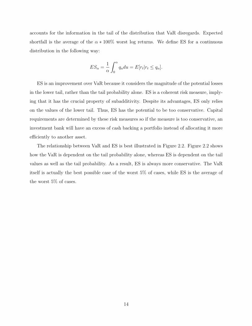
The relationship between VaR and ES is best illustrated in Figure 2.2. Figure 2.2 shows
how the VaR is dependent on the tail probability alone, whereas ES is dependent on the tail
values as well as the tail probability. As a result, ES is always more conservative. The VaR
itself is actually the best possible case of the worst 5% of cases, while ES is the average of
the worst 5% of cases.
14
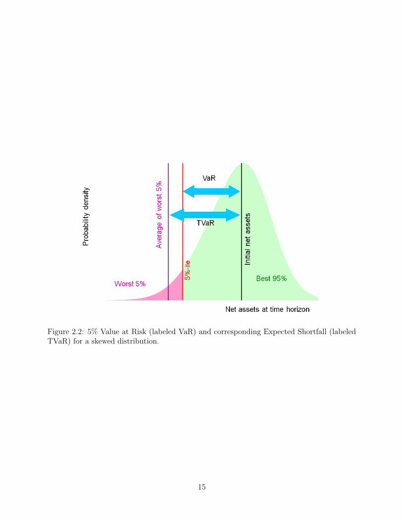
Figure 2.2: 5% Value at Risk (labeled VaR) and corresponding Expected Shortfall (labeledTVaR) for a skewed distribution.
15
Chapter 3
Expectiles
Chapter 3 explores the characteristics of expectiles that make them suitable for use as risk
measures in finance. The first section outlines the properties of expectiles. The second
section explains the interpretation of the expectile parameter, τ . The final section explains a
parametric method for generating a time-varying expectile, including underlying assumptions
and issues.
3.1 Properties
The term expectile was coined by Newey and Powell (1987) due to its dependence on the
properties of the expectation of the random variable Y conditional on Y being in a tail of
the distribution. The expectile relies on fundamentally different information to measure risk
since it is dependent on both tails of the distribution. Expected shortfall is sensitive to the
magnitude of the lower tail returns, but only those of the lower tail. As such, it tends to
be more conservative than other risk measures. VaR is not influenced by the magnitude of
lower tail returns at all, increasing the chance that it underestimates the true risk involved.
The expectile relies on more comprehensive information to measure risk.
16
The τ th expectile, µ(τ) minimizes
E[|τ − I(Y < m)|(Y −m)2] (3.1)
with respect to m for random variable Y and a given τ ∈ [0, 1]. The solution to the
minimization above, µ(τ), satisfies the expression
1− 2τ
τE[(Y − µ(τ))I(Y < µ(τ))] = µ(τ)− E[Y ]. (3.2)
The above expression is the method used to find the parametric expectile for the parametric
EVaR proposed in Section 3.3.
Given (y1, . . . , yn), the τ th sample expectile is found using asymmetric least squares (ALS)
minimization, defined as
min
[ n∑i=1
τ(yi −m)2I(yi≥m) + (1− τ)(yi −m)2
I(yi<m)
], with respect to m. (3.3)
First introduced by Newey and Powell (1987), this minimization is known as ALS regression
or weighted asymmetric least squares regression (LAWS). Note that if we take τ = 0.5,
LAWS actually reduces to ordinary least squares.
Examining the check-loss function of the expectile reveals many of the properties that
make it an attractive measure of risk. We can see from the check function that it weights
negative deviations using (1−τ) and positive deviations using τ . Weighting the positive and
negative deviations provides information about the symmetry of the distribution. Expectiles
yield more information about the heteroskedasticity of the distribution as well. The quadratic
loss function makes the expectile more sensitive to extreme values, and to the shape of the
distribution in general. As the expectile has the crucial property of subadditivity that the
quantile lacks, its primary advantage is that it is a coherent measure of risk (Satchell, 2010).
Some of the most important work on expectiles arise from the study of quantile regres-
sion. This comes from the relationship between asymmetric least squares regression and
quantile regression. To better understand this relationship, we introduce the check-loss for
17
the quantile:
E[|α− I(Y < m)||Y −m|],
where Y is a random variable and α ∈ [0, 1] The value of m that minimizes the expected value
for a given α is the quantile, qα. Quantile regression is similarly defined as the minimization,
with respect to m, of
minm
[ n∑1
α|yi −m|+ + (1− α)|yi −m|−].
From this perspective, we can see that ALS is the least squares analog of quantile regression.
Expectile regression has a similar advantage as quantile regression in that it can characterize
the shape of the distribution. The quantile is robust to extreme values, however, while the
expectile is not. This can be beneficial, since if we are measuring potential losses, we want
our measure to be sensitive to extreme tail losses. The expectile depends on the shape of the
entire distribution, while only the shape of the lower tail of the distribution affects quantiles.
One of the primary reasons researchers began to recognize the advantage of using ex-
pectiles was the fact that ALS regression is more computationally efficient than quantile
regression. Computing the expectile is simpler than computing the quantile because the
check-loss function is continuously differentiable.
The relationship between expectiles and quantiles encouraged the expectiles use in fi-
nance. Efron (1991) suggested estimating quantiles by the expectile for which the proportion
of in-sample observations lying below the expectile is τ . The one-to-one mapping between
quantiles and expectiles has been empirically supported by Jones (1994), Abdous and Remil-
lard (1995), and Yao and Tong (1996). Taylor (2008) estimated the nonparametric VaR and
Expected Shortfall via the expectile. The emphasis has generally been placed on the com-
putational efficiency of the expectile as compared to quantile regression, rather than on the
virtues of the expectile as a risk measure. De Rossi and Harvey (2009) were the first to
directly use the expectile by developing a spline-based nonparametric computation method
for the time-varying expectile. Its use was still limited by the difficulty in interpreting the
expectile and its asymmetry parameter. Direct use of the expectile as a risk measure has
18

been discouraged by the expectiles lack of interpretation. Kuan et al. (2009) addressed the
issue of interpretability by giving a more intuitive definition for the expectile in a financial
risk setting.
3.2 Interpretation
The most glaring issue with using expectiles is the difficulty in interpretation. This makes
the direct use of the expectile as a risk measure difficult to justify. Recently, however, an
interpretation for the expectile in terms of financial risk has been proposed by Kuan et al.
(2009). They introduced the asymmetry parameter, τ , as the index of prudentiality. Recall
that the margin or capital requirement is the amount of capital to be held in reserve for a
given set of assets. The level of prudentiality relies on the use of risk measures as capital
or margin requirements as it can be thought of as the relative cost of the expected margin
shortfall. This results from the expectile satisfying the expression
∫ µ(τ)
−∞ (y − µ(τ))dF (y)∫ µ(τ)
−∞ (y − µ(τ))dF (y) +∫∞µ(τ)
(y − µ(τ))dF (y)=
∫ µ(τ)
−∞ (y − µ(τ))dF (y)∫∞−∞(y − µ(τ))dF (y)
= τ, (3.4)
where µ(τ) is the τ th expectile and F (y) is the cumulative distribution of the random variable
Y . The denominator is the sum of∫ µ(τ)
−∞ (y−µ(τ))dF (y) and∫∞µ(τ)
(y−µ(τ))dF (y), which are
the expected margin shortfall and the opportunity cost due to expected margin overcharge,
respectively. Together they are the total expected cost of holding the capital requirement,
µ(τ). Thus, τ is the ratio of the expected margin shortfall to the expected total cost of
the capital requirement. Therefore, it is the relative cost of the expected margin shortfall.
Since the magnitude of µ(τ) represents the margin requirement, the greater the magnitude
of µ(τ), the smaller the expected shortfall, which results in a smaller τ.
Lower values of τ indicate more risk aversion. Kuan et al. (2009) suggest that the EVaR
can be thought of as a flexible VaR, since the tail probability associated with an expectile is
not some static α chosen at the outset, but changes with the underlying distribution. Table
3.1 contains the corresponding α of τ = 0.05 and τ = 0.01 for the Uniform(0,1), N(0,1), and
t(5) distributions. It illustrates that the probability α, associated with the τ th expectile is
19
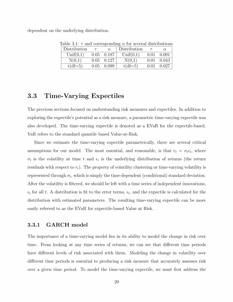
dependent on the underlying distribution.
Table 3.1: τ and corresponding α for several distributions.Distribution τ α Distribution τ α
Unif(0,1) 0.05 0.187 Unif(0,1) 0.01 0.091N(0,1) 0.05 0.127 N(0,1) 0.01 0.043t(df=5) 0.05 0.099 t(df=5) 0.01 0.027
3.3 Time-Varying Expectiles
The previous sections focused on understanding risk measures and expectiles. In addition to
exploring the expectile’s potential as a risk measure, a parametric time-varying expectile was
also developed. The time-varying expectile is denoted as a EVaR for the expectile-based.
VaR refers to the standard quantile based Value-at-Risk.
Since we estimate the time-varying expectile parametrically, there are several critical
assumptions for our model. The most essential, and reasonable, is that rt = σtεt, where
σt is the volatility at time t and εt is the underlying distribution of returns (the return
residuals with respect to rt). The property of volatility clustering or time-varying volatility is
represented through σt, which is simply the time-dependent (conditional) standard deviation.
After the volatility is filtered, we should be left with a time series of independent innovations,
εt for all t. A distribution is fit to the error terms, εt, and the expectile is calculated for the
distribution with estimated parameters. The resulting time-varying expectile can be more
easily referred to as the EVaR for expectile-based Value at Risk.
3.3.1 GARCH model
The importance of a time-varying model lies in its ability to model the change in risk over
time. From looking at any time series of returns, we can see that different time periods
have different levels of risk associated with them. Modeling the change in volatility over
different time periods is essential to producing a risk measure that accurately assesses risk
over a given time period. To model the time-varying expectile, we must first address the
20
change in volatility over time, i.e. volatility clustering. The ARCH (autoregressive condi-
tional heteroskedasticity) model was developed by Engle (1982) to model the conditional
heteroskedasticity in financial data sets. Bollerslev (1986) generalized this process to the
GARCH (generalized autoregressive conditional heteroskedasticity). The ARCH(k) process
takes advantage of the autocorrelation that exists between the previous q squared returns.
Autocorrelation among squared returns, but not among simple returns is a common statis-
tical property of financial data sets. The GARCH(p,q) process improves the estimation of
heteroskedasticity by including the conditional variances from the p previous time intervals.
Typically, we assume σt ∼ GARCH(1,1) because of the models simplicity and empirical
performance. Thus, the time-varying volatility is modeled as
σ2t = ω + β1r
2t−1 + β2σ
2t−1, (3.5)
where ω > 0 is a constant, β1 > 0 is the autoregressive coefficient, β2 > 0 is the lagged
conditional variance coefficient, and β1+β2 < 1. By estimating β1, β2, and ω, we can estimate
the time-varying volatility, σt. To test the GARCH(1,1) fit, we examine the plot the squared
GARCH residuals, ε̂2t . The Ljung-Box test is useful for determining if the residuals are
independently distributed. Checking the autocorrelation function of the squared GARCH
residuals and the Ljung-Box test statistic aid in assessing the appropriateness of the GARCH
model.
3.3.2 NIG distribution
After estimating the volatility the returns are devolatized by dividing rt by σ̂t, yielding ε̂t.
If the GARCH model fits well, then the resulting residual should be independently and
identically distributed. Historically, several distributions have been fit to the conditional
returns, including the normal distribution, Student’s t distribution, the skewed Student’s t
distribution, and the generalized hyperbolic distribution with varying success (Cont, 2001;
Hu and Kercheval, 2007). A special case of the generalized hyperbolic, the Normal Inverse
Gaussian(NIG) distribution, seems to model the heavy tails of this distribution well when
compared to previous attempts at distribution fitting (McNeil et al., 2005). The NIG dis-
21
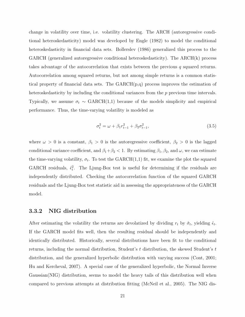
tribution has four parameters: µ (location), ξ (shape), β (asymmetry), and δ (scale). A
distribution with additional scale and skewness parameters, such as the NIG, can account
for the heavy tails and asymmetry common to financial returns distributions. Figure 3.1
several instances of the NIG distribution for different combinations of parameters.
−10 −5 0 5 10
0.0
0.1
0.2
0.3
0.4
0.5
0.6
Normal Inverse Gaussian Distributions
x
Den
sity
ξ = 1, β = 0, δ = 1, µ = 0ξ = 1, β = 0.99, δ = 1, µ = 0ξ = 0.01, β = 0, δ = 1, µ = 0ξ = 1, β = 0, δ = 10, µ = 0
Figure 3.1: NIG distributions with different parameters
Solving (3.2) using the NIG(µ̂, ξ̂, β̂, δ̂) density for a given τ yields µ̂(τ). To model the
EV aR, µ̂t(τ), the time-varying volatility must be factored in, which gives us µ̂t(τ) = σ̂tµ̂(τ).
For reference, the time-varying quantile for a given α ∈ [0, 1] was also calculated using the
fitted NIG distribution. The given quantile of the residual time series is multiplied by the
appropriate volatility at time t to generate the time-varying quantile-based VaR, V aRα.
22

Chapter 4 explores the relationship between quantiles and expectiles, compares the afore-
mentioned parametric method for estimating expectiles with the LAWS estimation method,
and provides real examples of the EVaR.
23
Chapter 4
Numerical Analysis
Chapter 4 explores the characteristics of expectiles and the EVaR using simulations and
application of the aforementioned EVaR estimation method. The first section consists of the
simulations designed to explore the relationship between the expectile and quantile as well as
general characteristics of the expectile. The second and final section covers the application
of the EVaR to the DIA, an ETF of the Dow Jones Industrial Average.
4.1 Simulation
4.1.1 Parametric Expectile vs. Sample Expectile
The following simulations were designed to test the robustness of the assumption of NIG
errors. The conditional standard deviation portion of the returns was generated by simulating
σt with a GARCH(1,1) model with coefficients ω = 0.05, β1 = 0.2, and β2 = 0.4. The
errors, εt, of the returns were random deviates from either the NIG(0,1,0,1), N(0,1), or
t(df=5). The GARCH(1,1) model was fit to the simulated returns and then the residuals
were used to estimate the parameters for an NIG distribution. The parametric expectile was
calculated using an NIG distribution with the estimated parameters. The sample expectile
was determined using the LAWS method performed on the residuals of the GARCH fit.
The expectile from the true distribution was then subtracted from the expectile estimated
parametrically and the sample expectile. The simulation consisted of 1000 generations of
24
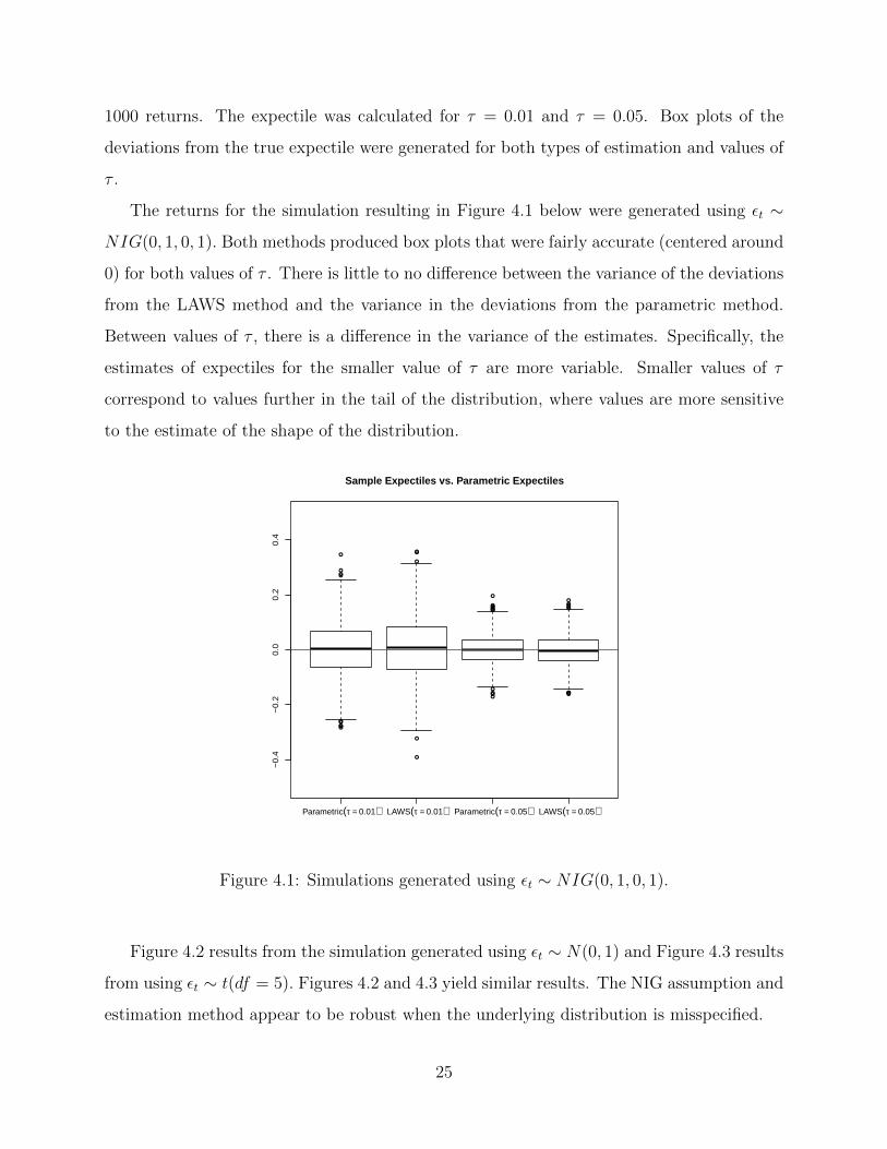
1000 returns. The expectile was calculated for τ = 0.01 and τ = 0.05. Box plots of the
deviations from the true expectile were generated for both types of estimation and values of
τ .
The returns for the simulation resulting in Figure 4.1 below were generated using εt ∼
NIG(0, 1, 0, 1). Both methods produced box plots that were fairly accurate (centered around
0) for both values of τ . There is little to no difference between the variance of the deviations
from the LAWS method and the variance in the deviations from the parametric method.
Between values of τ , there is a difference in the variance of the estimates. Specifically, the
estimates of expectiles for the smaller value of τ are more variable. Smaller values of τ
correspond to values further in the tail of the distribution, where values are more sensitive
to the estimate of the shape of the distribution.
●
●
●●●●
●●
●
●
●
●
●
●
●
●
●●●●
●
●
●
●
●
●
●
●
●
●●
●
●
●
●
●
●●
Parametric(τ = 0.01) LAWS(τ = 0.01) Parametric(τ = 0.05) LAWS(τ = 0.05)
−0.
4−
0.2
0.0
0.2
0.4
Sample Expectiles vs. Parametric Expectiles
Figure 4.1: Simulations generated using εt ∼ NIG(0, 1, 0, 1).
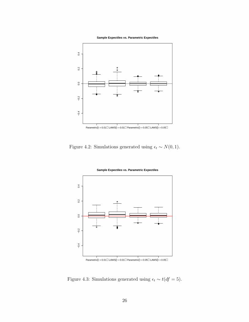
Figure 4.2 results from the simulation generated using εt ∼ N(0, 1) and Figure 4.3 results
from using εt ∼ t(df = 5). Figures 4.2 and 4.3 yield similar results. The NIG assumption and
estimation method appear to be robust when the underlying distribution is misspecified.
25
●●●
●
●
●
●●
●●
●
●
●
●
●●●
● ●
●●●
●
●
Parametric(τ = 0.01) LAWS(τ = 0.01) Parametric(τ = 0.05) LAWS(τ = 0.05)
−0.
4−
0.2
0.0
0.2
0.4
Sample Expectiles vs. Parametric Expectiles
Figure 4.2: Simulations generated using εt ∼ N(0, 1).
● ●
●
●●●●●
●●●●●
Parametric(τ = 0.01) LAWS(τ = 0.01) Parametric(τ = 0.05) LAWS(τ = 0.05)
−0.
4−
0.2
0.0
0.2
0.4
Sample Expectiles vs. Parametric Expectiles
Figure 4.3: Simulations generated using εt ∼ t(df = 5).
26
4.1.2 Sample Quantile vs. Sample Expectile
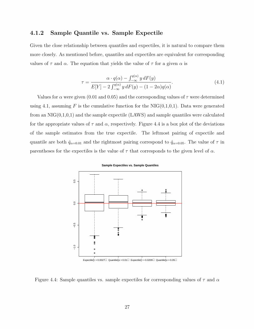
Given the close relationship between quantiles and expectiles, it is natural to compare them
more closely. As mentioned before, quantiles and expectiles are equivalent for corresponding
values of τ and α. The equation that yields the value of τ for a given α is
τ =α · q(α)−
∫ q(α)
−∞ y dF (y)
E[Y ]− 2∫ q(α)
−∞ y dF (y)− (1− 2α)q(α). (4.1)
Values for α were given (0.01 and 0.05) and the corresponding values of τ were determined
using 4.1, assuming F is the cumulative function for the NIG(0,1,0,1). Data were generated
from an NIG(0,1,0,1) and the sample expectile (LAWS) and sample quantiles were calculated
for the appropriate values of τ and α, respectively. Figure 4.4 is a box plot of the deviations
of the sample estimates from the true expectile. The leftmost pairing of expectile and
quantile are both q̂α=0.01 and the rightmost pairing correspond to q̂α=0.05. The value of τ in
parentheses for the expectiles is the value of τ that corresponds to the given level of α.
●
●
●
●
●
●
●
●
●
●
●
●
●
●●●
●
●
●●●●●
●
●
●●
●
●●
●
●
●●●
●
●
Expectile(τ = 0.0027) Quantile(α = 0.01) Expectile(τ = 0.0209) Quantile(α = 0.05)
−1.
0−
0.5
0.0
0.5
Sample Expectiles vs. Sample Quantiles
Figure 4.4: Sample quantiles vs. sample expectiles for corresponding values of τ and α
27
The sample quantile and sample expectile were both very accurate. The sample expec-
tile deviations for α = 0.01 are more variable, which is a result of the sample expectile’s
sensitivity to extreme values. Again, we see that as τ and α increase, the variances of the
deviations decrease for both estimators.
4.2 Real Data
4.2.1 Dow Jones Industrial Average
The following analysis consists of 1018 closing day prices the Dow Jones Industrial Average
Exchange Traded Fund (ETF) taken from January 2, 2008 to January 13, 2012. This section
outlines the process used to generate the EVaR.
The GARCH(1,1) fit was assessed using the autocorrelation function (ACF) of the
squared GARCH residuals, in addition to the Box-Ljung test. The NIG fit was evalu-
ated by examining the shape of the histogram of the GARCH residuals, as well as a NIG
QQ-plot and fit plot. Additional figures used to evaluate assumptions and fit of the model
are included in Appendix A.1.
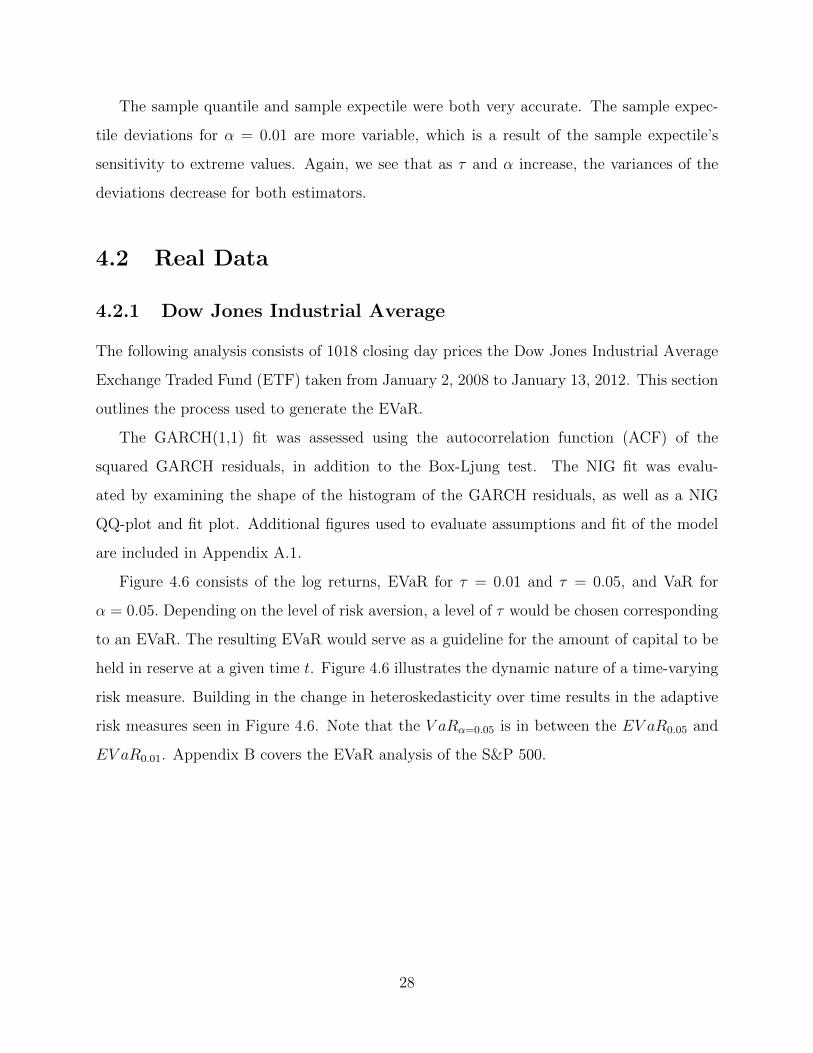
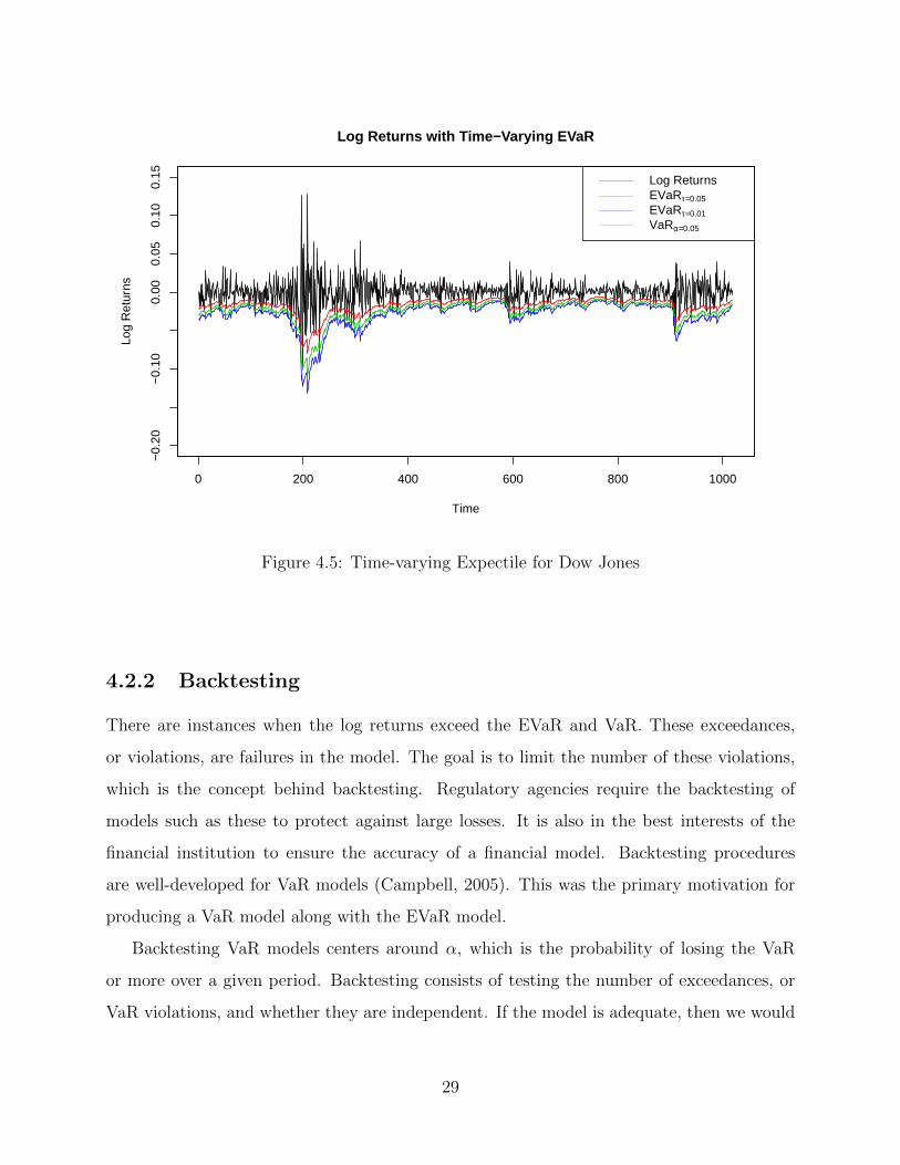
Figure 4.6 consists of the log returns, EVaR for τ = 0.01 and τ = 0.05, and VaR for
α = 0.05. Depending on the level of risk aversion, a level of τ would be chosen corresponding
to an EVaR. The resulting EVaR would serve as a guideline for the amount of capital to be
held in reserve at a given time t. Figure 4.6 illustrates the dynamic nature of a time-varying
risk measure. Building in the change in heteroskedasticity over time results in the adaptive
risk measures seen in Figure 4.6. Note that the V aRα=0.05 is in between the EV aR0.05 and
EV aR0.01. Appendix B covers the EVaR analysis of the S&P 500.
28
0 200 400 600 800 1000
−0.
20−
0.10
0.00
0.05
0.10
0.15
Time
Log
Ret
urns
Log Returns with Time−Varying EVaR
Log ReturnsEVaRτ=0.05
EVaRτ=0.01
VaRα=0.05
Figure 4.5: Time-varying Expectile for Dow Jones
4.2.2 Backtesting
There are instances when the log returns exceed the EVaR and VaR. These exceedances,
or violations, are failures in the model. The goal is to limit the number of these violations,
which is the concept behind backtesting. Regulatory agencies require the backtesting of
models such as these to protect against large losses. It is also in the best interests of the
financial institution to ensure the accuracy of a financial model. Backtesting procedures
are well-developed for VaR models (Campbell, 2005). This was the primary motivation for
producing a VaR model along with the EVaR model.
Backtesting VaR models centers around α, which is the probability of losing the VaR
or more over a given period. Backtesting consists of testing the number of exceedances, or
VaR violations, and whether they are independent. If the model is adequate, then we would
29
expect the proportion of VaR exceedances to be close to α. Testing this idea, known as
unconditional coverage, assumes that the number of violations, N , is binomially distributed
with E[N ] = Tα, where T is the total number of time points. Independence of exceedances
is also desired as it guarantees against clustering of VaR violations. The test statistic for
testing the simultaneous null hypothesis
H0 : E[N ] = Tα,Violations are independent.
can be found in Appendix C (Jeong and Kang, 2009; Hamidi et al., 2010).
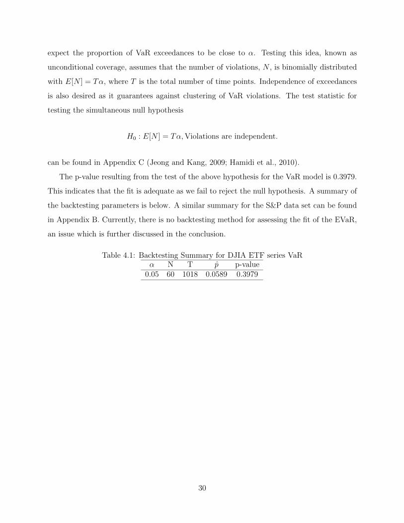
The p-value resulting from the test of the above hypothesis for the VaR model is 0.3979.
This indicates that the fit is adequate as we fail to reject the null hypothesis. A summary of
the backtesting parameters is below. A similar summary for the S&P data set can be found
in Appendix B. Currently, there is no backtesting method for assessing the fit of the EVaR,
an issue which is further discussed in the conclusion.
Table 4.1: Backtesting Summary for DJIA ETF series VaRα N T p̂ p-value
0.05 60 1018 0.0589 0.3979
30
Chapter 5
Conclusions and Future Work
Expectiles have great potential in analyzing risk in finance. The expectile exhibits properties
that satisfy the axioms of coherence, an essential given our current understanding of risk.
The ALS estimator is accurate and computationally efficient. The expectile can be used to
directly estimate quantiles and, thus, VaR. The expectile fully characterizes the underlying
distribution and takes advantage of more information than competing risk measures. τ
becomes better understood and backtesting methods are developed, expectiles will become
accepted measures of risk.
The expectile has its share of issues and more research is needed, particularly in the
area of backtesting. Since α is a probability and a proportion, it is relatively simple to
backtest. The level of prudentiality, τ , has an interpretation that does not lend itself to
backtesting. Currently, the lack of a backtesting procedure limits the expectile’s use in
finance to estimating the quantile in VaR models.This is probably why the most promising
work has been in the relationship between the expectile and the quantile.
The relationship between the quantile and expectile is yet to be studied thoroughly. It
is yet to be known whether the sample expectile is more efficient at estimating the sample
quantile in many cases. The remaining work in this area appears to be theoretical rather
than applied.
Even if we concede the lack of backtesting, there is more to be done with expectiles.
Potentially, the expectile can be used to rank portfolios according to risk aversion. The
31
expectile could be used in portfolio optimization by selecting for a given level of prudentiality
and returning the portfolio that best fits the desired risk aversion profile.
The field of finance will continue to search for a measure of risk that is coherent, inter-
pretable, efficient, accurate, and robust. The expectile satisfies several of these demands.
Perhaps, with a little work, the expectile will be the primary risk measure of financial insti-
tutions of the future.
32
Appendix A
Additional Results for DJIA analysis
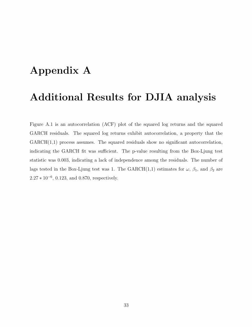
Figure A.1 is an autocorrelation (ACF) plot of the squared log returns and the squared
GARCH residuals. The squared log returns exhibit autocorrelation, a property that the
GARCH(1,1) process assumes. The squared residuals show no significant autocorrelation,
indicating the GARCH fit was sufficient. The p-value resulting from the Box-Ljung test
statistic was 0.003, indicating a lack of independence among the residuals. The number of
lags tested in the Box-Ljung test was 1. The GARCH(1,1) estimates for ω, β1, and β2 are
2.27 ∗ 10−6, 0.123, and 0.870, respectively.
33
0 5 10 15 20 25 30
0.0
0.4
0.8
Lag
ACF
ACF of Squared stock
0 5 10 15 20 25 30
0.0
0.4
0.8
Lag
ACF
ACF of Squared Residuals
Figure A.1: ACF of Squared Returns and Squared Residuals
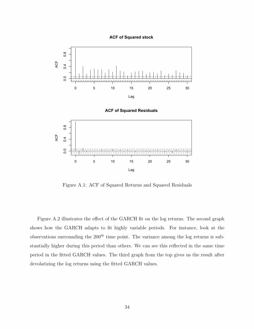
Figure A.2 illustrates the effect of the GARCH fit on the log returns. The second graph
shows how the GARCH adapts to fit highly variable periods. For instance, look at the
observations surrounding the 200th time point. The variance among the log returns is sub-
stantially higher during this period than others. We can see this reflected in the same time
period in the fitted GARCH values. The third graph from the top gives us the result after
devolatizing the log returns using the fitted GARCH values.
34
Log Returns
time
log−
retu
rn
0 200 400 600 800 1000
−0.
100.
05
0 200 400 600 800 1000
0.01
0.04
Fitted GARCH values
Index
fitte
d
GARCH residuals
Time
err
0 200 400 600 800 1000
−4
02
Figure A.2: Log Returns, Fitted GARCH values, and GARCH residuals for Dow Jones data
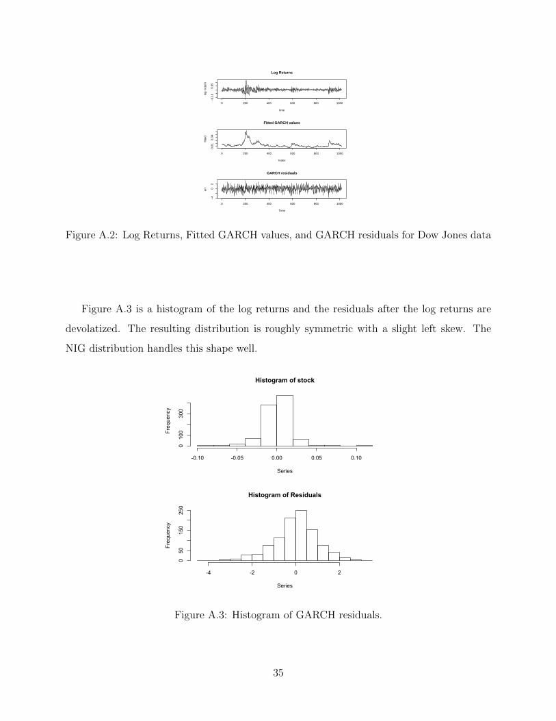
Figure A.3 is a histogram of the log returns and the residuals after the log returns are
devolatized. The resulting distribution is roughly symmetric with a slight left skew. The
NIG distribution handles this shape well.
Histogram of stock
Series
Frequency
-0.10 -0.05 0.00 0.05 0.10
0100
300
Histogram of Residuals
Series
Frequency
-4 -2 0 2
050
150
250
Figure A.3: Histogram of GARCH residuals.
35
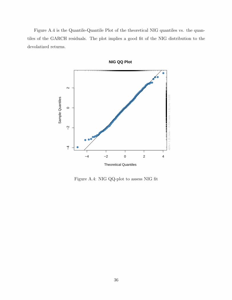
Figure A.4 is the Quantile-Quantile Plot of the theoretical NIG quantiles vs. the quan-
tiles of the GARCH residuals. The plot implies a good fit of the NIG distribution to the
devolatized returns.
●
● ● ●●●●●●●
●●●●●
●●●●●●●●●●●●●●
●●●●●●●●●●●●●●●●●
●●●●●●●●●●●●●●●●●●●●●●●●●●●●●●●●●●●●●●●●●●●●●●●●●●●●●●●●●●●●●●●●●●●●●●●●●●●●●●●●●●●●●●●●●●●●●●●●●●●●●●●●●●●●●●●●●●●●●●●●●●●●●●●●●●●●●●●●●●●●●●●●●●●●●●●●●●●●●●●●●●●●●●●●●●●●●●●●●●●●●●●●●●●●●●●●●●●●●●●●●●●●●●●●●●●●●●●●●●●●●●●●●●●●●●●●●●●●●●●●●●●●●●●●●●●●●●●●●●●●●●●●●●●●●●●●●●●●●●●●●●●●●●●●●●●●●●●●●●●●●●●●●●●●●●●●●●●●●●●●●●●●●●●●●●●●●●●●●●●●●●●●●●●●●●●●●●●●●●●●●●●●●●●●●●●●●●●●●●●●●●●●●●●●●●●●●●●●●●●●●●●●●●●●●●●●●●●●●●●●●●●●●●●●●●●●●●●●●●●●●●●●●●●●●●●●●●●●●●●
●●●●●●●●●●●●●●●●●●●●●●●●●●●●●●●●●●●●●●●●●●●●●●●●●●●●●●●●●●●●●●●●●●●●●●●●●●●●●●●●●●●●●●●●●●●●●●●●●●●●●●●●●●●●●●●●●●●●●●●●●●●●●●●●●●●●●●●●●●●●●●●●●●●●●●●●●●●●●●●●●●●●●●●●●●●●●●●●●●●●●●●●●●●●●●●●●●●●●●●●●●●●●●●●●●●●●●●●●●●●●●●●●●●●●●●●●●●●●●●●●●●●●●●●●●●●●●●●●●●●●●●●●●●●●●●●●●●●●●●●●●●●●●●●●
●●●●●●●●●●●●●●●●●●●●●●●●●●●●●●●●●●●●●●●●●●●●●●●●●●●●●●●●●●●●●●●●●●●●●●●●●●●●●●●●●●●●●●●●●●●●●●●●●●●●●●●●●●●●●●●●●●●●●●●●●●●●●●●●●●●●●●●●●●●●●●●●●●●●●●●●●●●●●●●●●●●●●●●●●●●●●●●●●●●●
●●●●●●●●●●●●●●●●●●●●●●
●●●●●●●●●●
●●●●●●●●
●● ●
●
−4 −2 0 2 4
−4
−2
02
Theoretical Quantiles
Sam
ple
Qua
ntile
sNIG QQ Plot
alph
a =
1.3
5 | b
eta
= −
0.22
4 | d
elta
= 1
.32
| mu
= 0
.229
Figure A.4: NIG QQ-plot to assess NIG fit
36
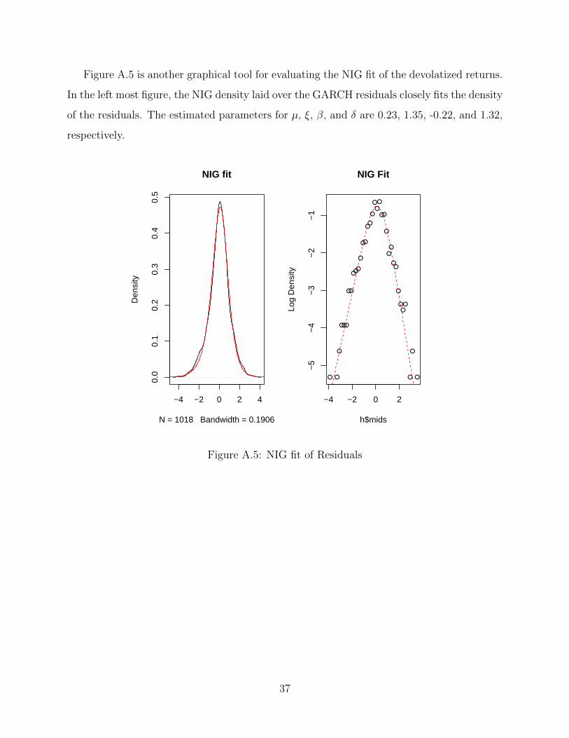
Figure A.5 is another graphical tool for evaluating the NIG fit of the devolatized returns.
In the left most figure, the NIG density laid over the GARCH residuals closely fits the density
of the residuals. The estimated parameters for µ, ξ, β, and δ are 0.23, 1.35, -0.22, and 1.32,
respectively.
−4 −2 0 2 4
0.0
0.1
0.2
0.3
0.4
0.5
NIG fit
N = 1018 Bandwidth = 0.1906
Den
sity
● ●
●
●●●
●●
●●●
●
●●
●●
●
●●
●
●●
●
●
●
●●
●
●●●
●
●
●
−4 −2 0 2
−5
−4
−3
−2
−1
NIG Fit
h$mids
Log
Den
sity
Figure A.5: NIG fit of Residuals
37
Appendix B
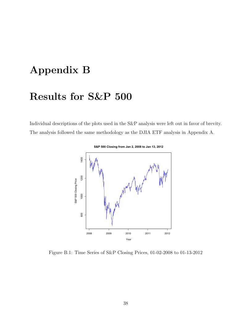
Results for S&P 500
Individual descriptions of the plots used in the S&P analysis were left out in favor of brevity.
The analysis followed the same methodology as the DJIA ETF analysis in Appendix A.
2008 2009 2010 2011 2012
800
1000
1200
1400
Year
S&
P 5
00 C
losi
ng P
rice
S&P 500 Closing from Jan 2, 2008 to Jan 13, 2012
Figure B.1: Time Series of S&P Closing Prices, 01-02-2008 to 01-13-2012
38
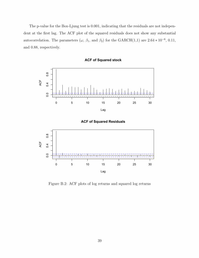
The p-value for the Box-Ljung test is 0.001, indicating that the residuals are not indepen-
dent at the first lag. The ACF plot of the squared residuals does not show any substantial
autocorrelation. The parameters (ω, β1, and β2) for the GARCH(1,1) are 2.64 ∗ 10−6, 0.11,
and 0.88, respectively.
0 5 10 15 20 25 30
0.0
0.4
0.8
Lag
ACF
ACF of Squared stock
0 5 10 15 20 25 30
0.0
0.4
0.8
Lag
ACF
ACF of Squared Residuals
Figure B.2: ACF plots of log returns and squared log returns
39
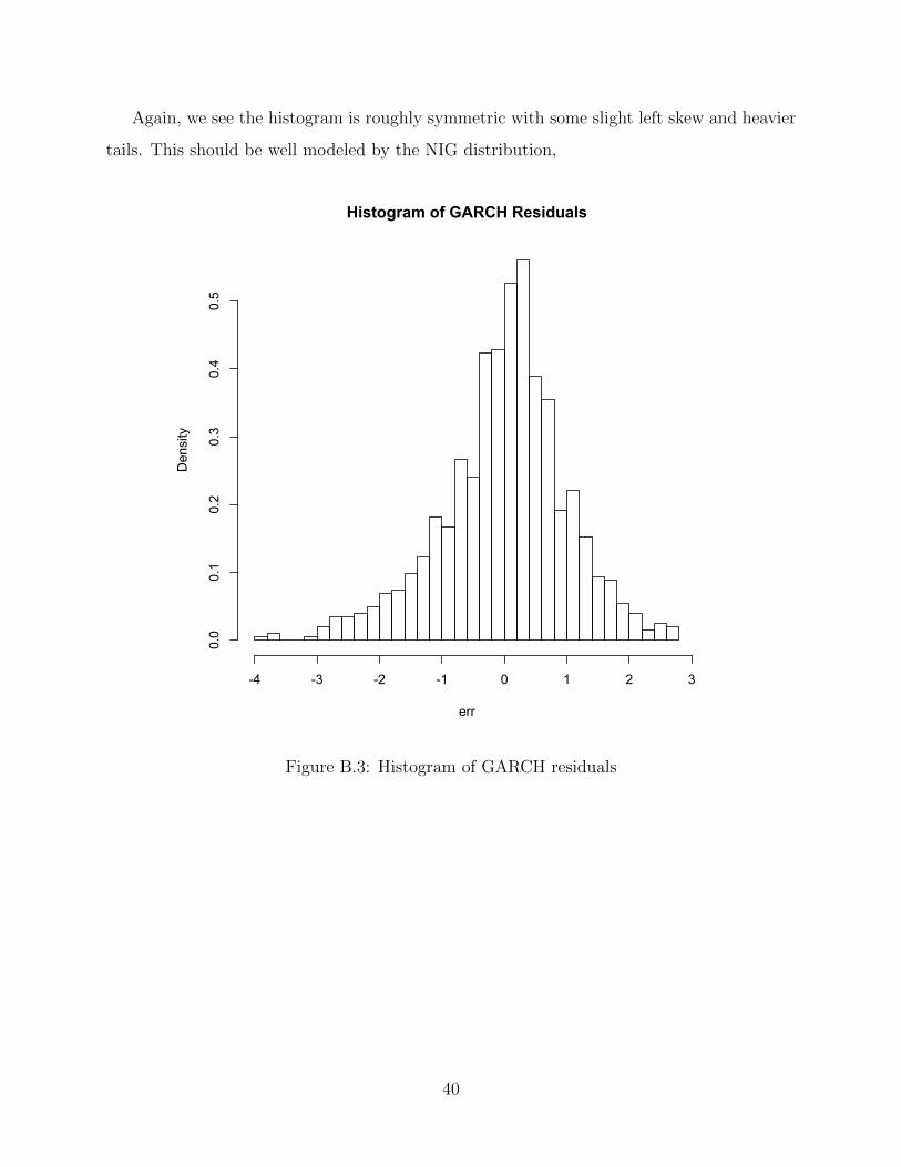
Again, we see the histogram is roughly symmetric with some slight left skew and heavier
tails. This should be well modeled by the NIG distribution,
Histogram of GARCH Residuals
err
Density
-4 -3 -2 -1 0 1 2 3
0.0
0.1
0.2
0.3
0.4
0.5
Figure B.3: Histogram of GARCH residuals
40
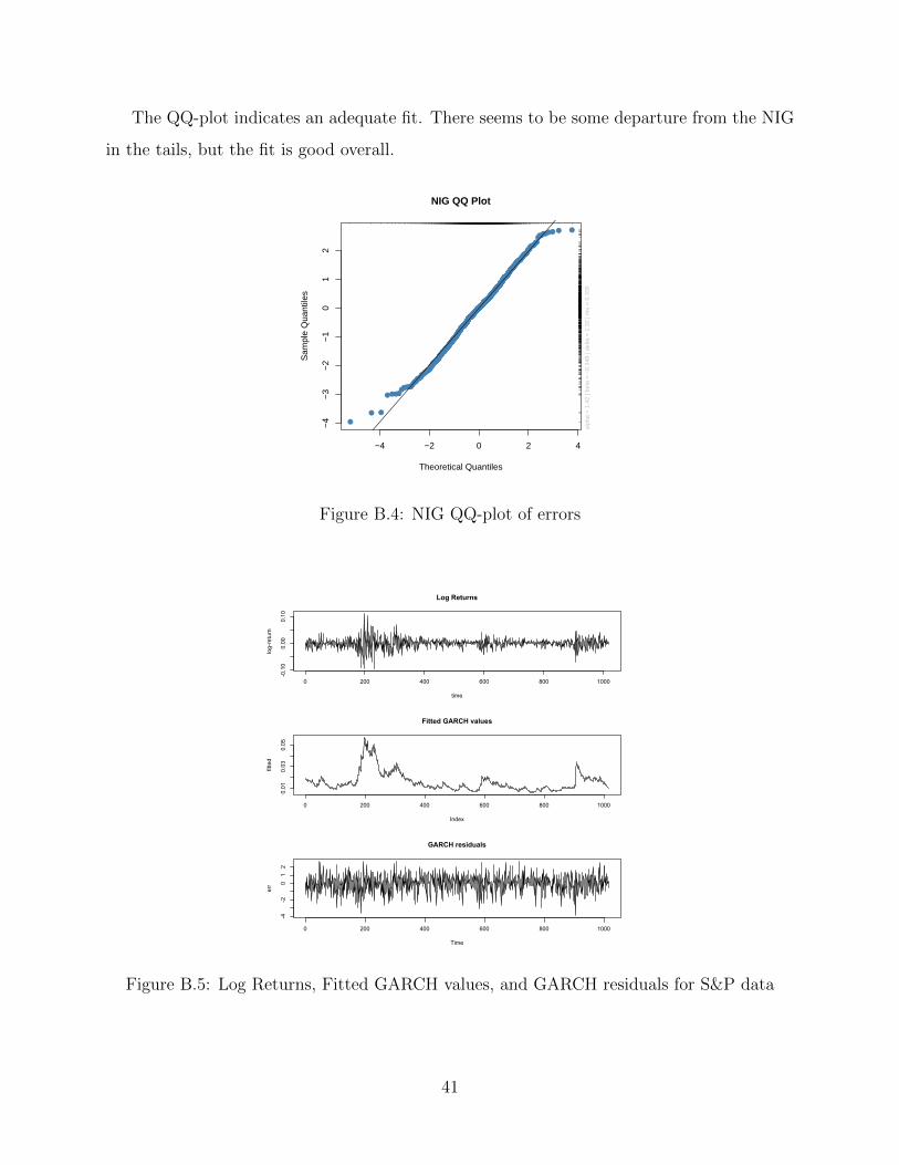
The QQ-plot indicates an adequate fit. There seems to be some departure from the NIG
in the tails, but the fit is good overall.
●
● ●
●●●●●●●●●●
●●●●●
●●●●●●●●●
●●●●●●●●●●●●●●●●●●●●●●●●●●●
●●●●●●●●●●●●●●●●●●●●●●●●●●●●●●●●●●●●●●●●●●●●●●●●●●●●●●●●●●●●●●●●●●●●●●●●●●●●●●●●●●●●●●●●●●●●●●●●●●●●●●●●●●●●●●●●●●●●●●●●●●●●●●●●●●●●●●●●●●●●●●●●●●●●●●●●●●●●●●●●●●●●●●●●●●●●●●●●●●●●●●●●●●●●●●●●●●●●●●●●●●●●●●●●●●●●●●●●●●●●●●●●●●●●●●●●●●●●●●●●●●●●●●●●●●●●●●●●●●●●●●●●●●●●●●●●●●●●●●●●●●●●●●●●●●●●●●●●●●●●●●●
●●●●●●●●●●●●●●●●●●●●●●●●●●●●●●●●●●●●●●●●●●●●●●●●●●●●●●●●●●●●●●●●●●●●●●●●●●●●●●●●●●●●●●●●●●●●●●●●●●●●●●●●●●●●●●●●●●●●●●●●●●●●●●●●●●●●●●●●●●●●●●●●●●●●●●●●●●●●●●●●●●●●●●●●●●●●●●●●●●●●●●●●●●●●●●●●●●●●●●●●●●●●●●●●●●●●●●●●●●●●●●●●●●●●●●●●●●●●●●●●●●●●●●●●●●●●●●●●●●●●●●●●●●●●●●●●●●●●●●●●●●●●●●●●●●●●●●●●●●●●●●●●●●●●●●●●●●●●●●●●●●●●●●●●●●●●●●●●●●●●●●●●●●●●●●●●●●●●●●●●●●●●●●●●●●●●●●●●●●●●●●●●●●●●●●●●●●●●●●●●●●●●●●●●●●●●●●●●●●●●●●●●●●●●●●●●●●●●●●●●●●●●●●●●●●●●●●●●●●●●●●●●●●●●●●●●●●●●●●●●●●●●●●●●●●●●●●●●●●●●●●●●●●●●●●●●●●●●●●●●●●●●●●●●●●●●●●●●●●●●●●●●●●●●●●●●●●●●●●●●●●●●●●●●●●●●●●●●●●●●●●●●●●●●●●●●●●●●●●●●●●●●●●●●●●●●●●●●●●●●●●●
●●●●●●●●●●●●●●
●●●●●●●●●●●
●●●●●
●●●● ● ●
−4 −2 0 2 4
−4
−3
−2
−1
01
2
Theoretical Quantiles
Sam
ple
Qua
ntile
s
NIG QQ Plot
alph
a =
1.4
2 | b
eta
= −
0.34
8 | d
elta
= 1
.32
| mu
= 0
.335
Figure B.4: NIG QQ-plot of errors
Log Returns
time
log-return
0 200 400 600 800 1000
-0.10
0.00
0.10
0 200 400 600 800 1000
0.01
0.03
0.05
Fitted GARCH values
Index
fitted
GARCH residuals
Time
err
0 200 400 600 800 1000
-4-2
012
Figure B.5: Log Returns, Fitted GARCH values, and GARCH residuals for S&P data
41
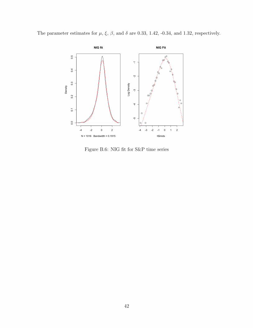
The parameter estimates for µ, ξ, β, and δ are 0.33, 1.42, -0.34, and 1.32, respectively.
-4 -2 0 2
0.0
0.1
0.2
0.3
0.4
0.5
NIG fit
N = 1016 Bandwidth = 0.1915
Density
-4 -3 -2 -1 0 1 2
-5-4
-3-2
-1
NIG Fit
h$mids
Log
Den
sity
Figure B.6: NIG fit for S&P time series
42
0 200 400 600 800 1000
−0.
20−
0.10
0.00
0.05
0.10
0.15
Time
Log
Ret
urns
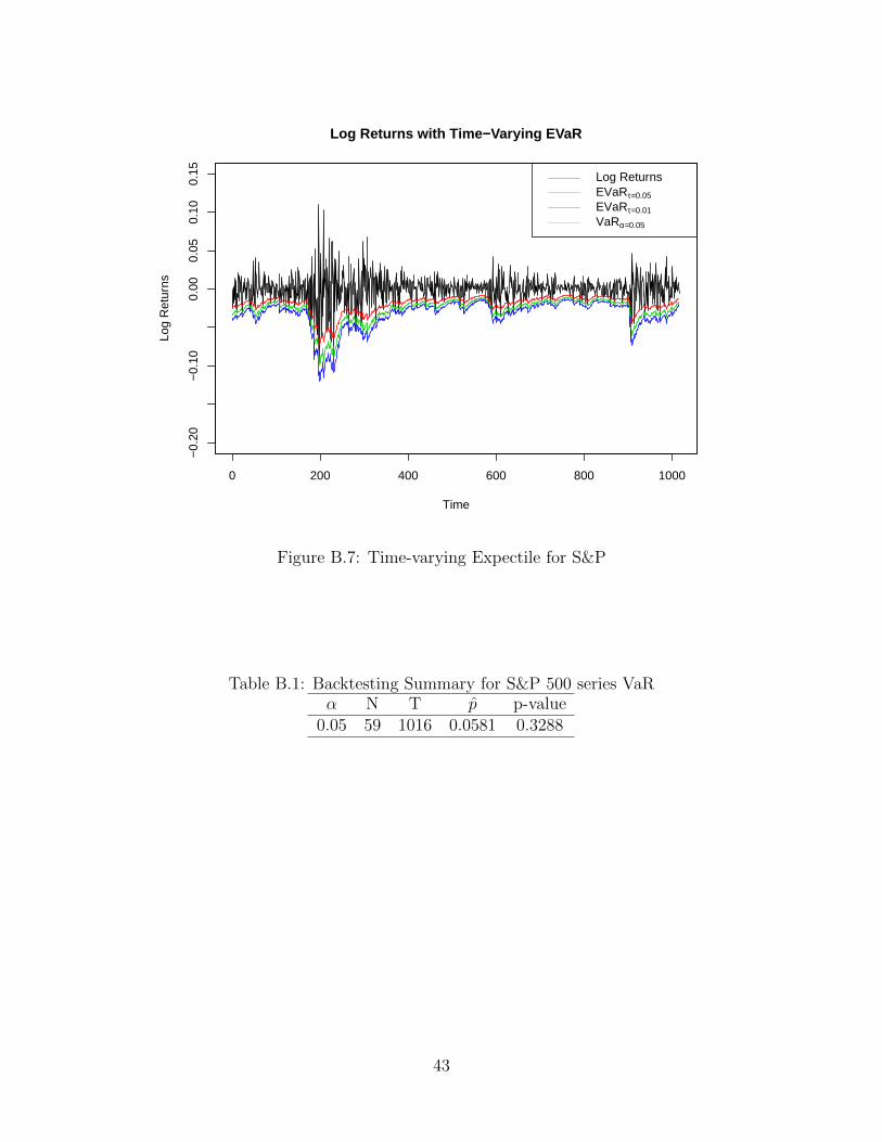
Log Returns with Time−Varying EVaR
Log ReturnsEVaRτ=0.05
EVaRτ=0.01
VaRα=0.05
Figure B.7: Time-varying Expectile for S&P
Table B.1: Backtesting Summary for S&P 500 series VaRα N T p̂ p-value
0.05 59 1016 0.0581 0.3288
43
Appendix C
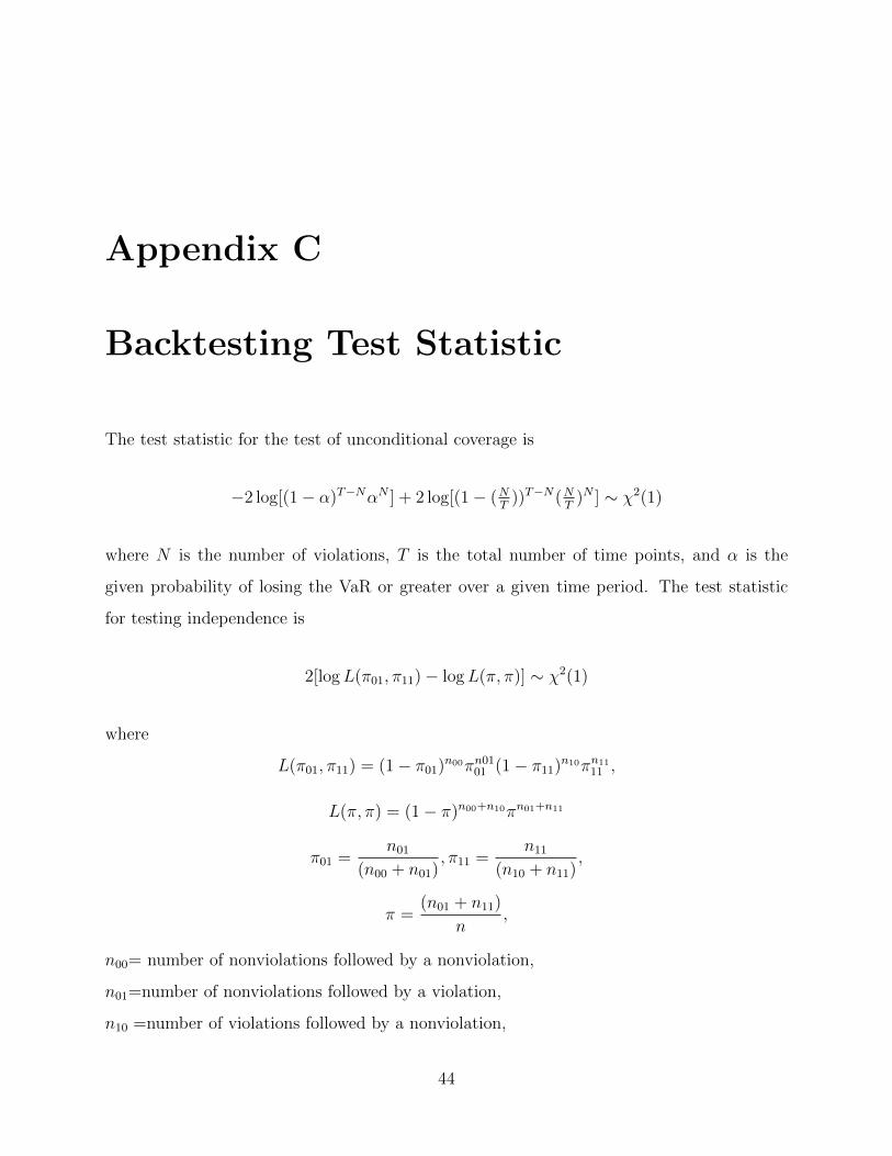
Backtesting Test Statistic
The test statistic for the test of unconditional coverage is
−2 log[(1− α)T−NαN ] + 2 log[(1− (NT
))T−N(NT
)N ] ∼ χ2(1)
where N is the number of violations, T is the total number of time points, and α is the
given probability of losing the VaR or greater over a given time period. The test statistic
for testing independence is
2[logL(π01, π11)− logL(π, π)] ∼ χ2(1)
where
L(π01, π11) = (1− π01)n00πn0101 (1− π11)n10πn11
11 ,
L(π, π) = (1− π)n00+n10πn01+n11
π01 =n01
(n00 + n01), π11 =
n11
(n10 + n11),
π =(n01 + n11)
n,
n00= number of nonviolations followed by a nonviolation,
n01=number of nonviolations followed by a violation,
n10 =number of violations followed by a nonviolation,
44

and n11 = number of violations followed by violations. Assuming the test statistics are
independent allows us to combine the two, yielding an overall test statistic that is distributed
χ2(2).
45
Appendix D
Bibliography
Abdous, B. and Remillard, B. (1995). Relating quantiles and expectiles under weighted-
symmetry. Annals of the Institute of Statistical Mathematics, 47(2):371–384.
Artzner, P., Delbaen, F., Eber, J.-M., and Heath, D. (1999). Coherent Measures of Risk.
Mathematical Finance, 9(3):203–228.
Bollerslev, T. (1986). Generalized autoregressive conditional heteroskedasticity. Journal of
Econometrics, 31:307–327.
Campbell, S. D. (2005). A review of backtesting and backtesting procedures. Finance and
Economics Discussion Series, 2005-21.
Cont, R. (2001). Empirical properties of asset returns: Stylized facts and statistical issues.
Quantitative Finance, 1:223–236.
De Rossi, G. and Harvey, A. C. (2009). Quantiles, expectiles, and splines. Journal of
Econometrics, 152(2):179–185.
Efron, B. (1991). Regression percentiles using asymmetric squared error loss. Statistica
Sinica, 1:93–125.
Engle, R. (1982). Autoregressive conditional heteroscedasticity with estimates of variance of
united kingdom inflation. Econometrica, 50:987–1008.
46
Engle, R. (2001). Garch 101: The use of arch/garch models in applied econometrics. Journal
of Economic Perspectives, 15(4):157–168.
Granger, C. and Poon, S.-H. (2003). Forecasting volatility in financial markets: A review.
Journal of Economic Literature, 41:478–539.
Granger, C. W. J. and Sin, C.-Y. (2000). Modelling the absolute returns of different stock
indices: exploring the forecastability of an alternative measure of risk. Journal of Fore-
casting, 19(4):277–298.
Hamidi, B., Kouontchou, P., and Maillet, B. (2010). Towards a well-diversified risk measure:a
dare approach. Revue Economique, 61(3):635–644.
Hu, W. and Kercheval, A. (2007). The skewed t distribution for portfolio credit risk. Advances
in Econometrics.
Jeong, S.-O. and Kang, K.-H. (2009). Nonparametric estimation of value-at-risk. Journal of
Applied Statistics, 36(11):1225–1238.
Jones, B. (1994). Expectiles and m-quantiles are quantiles. Statistics Letters, 20:149–153.
Koenker, R. and Hallock, K. F. (2001). Quantile regression. Journal of Economic Perspec-
tives, 15(4):143–156.
Kuan, C.-M., Yeh, J., and Hsu, Y.-C. (2009). Assessing value at risk with care, the condi-
tional autoregressive expectile models. Journal of Econometrics, 150(2):261–270.
McNeil, A., Frey, R., and Embrechts, P. (2005). Quantitative Risk Management: Concepts,
Techniques and Tools. Princeton University Press, 1 edition.
Newey, W. K. and Powell, J. L. (1987). Asymmetric least squares estimation and testing.
Econometrica, 55(4):819–847.
Satchell, S. (2010). Optimizing Optimization: The Next Generation of Optimization, Appli-
cations and Theory. Academic Press Press, 1 edition.
47
Taylor, J. W. (2008). Estimating value at risk and expected shortfall using expectiles. Journal
of Financial Econometrics, 6:231–252.
Yamai, Y. and Yoshiba, T. (2002). Comparative analyses of expected shortfall and value-
at-risk (2): Expected utility maximization and tail risk. Monetary and Economic Studies,
20:95–115.
Yao, Q. and Tong, H. (1996). Asymmetric least squares regression estimation: A nonpara-
metric approach. Journal of Nonparametric Statistics, 6(2-3):273–292.
48