A STUDY ON THE METHODS FOR

PERFORMANCE DESIGN AND IMPROVEMENT

IN COLLABORATIVE SYSTEMS

Tad Gonsalves C0171001

Information and Systems Engineering Laboratory, Faculty of Science & Technology,

Sophia University, Tokyo, JAPAN

Abstract In the conventional system development life cycle (SDLC), system performance and evaluation phase comes after the implementation phase. The aim of this research is to project system performance estimate at the requirement analysis and design phase itself, much before the implementation phase. This study introduces novel tools for modelling the system, evaluating the performance of the system and for improving and enhancing its performance. The types of systems that have been chosen as the object of this study are collaborative systems. In particular, wide-scale inter-collaboration, intra-collaboration and micro-level collaboration within the subsystem engaged in collaboration are analyzed, modelled and their performance is evaluated and improved.

Different scenarios of collaborative activity are being examined in detail. At the centre of each scenario is a server model that seeks to represent a particular type of service in collaborative systems. Single and parallel servers model the general type of collaborative activity. Distributed type of service occurs when the same service providing unit (SPU) has to devote itself to a series of tasks. The shifting of the SPUs from server to server, offering service, is best represented visually by Petri nets. The performance of the system represented by Petri nets can also be evaluated and improved qualitatively.

Collaborative systems, being client-server in nature, are modelled by using Multi-Context Map (MCM) technique. System evaluation is through GPSS simulation and improvement is by the Expert System reasoning with qualitative rules. MCM captures the workflow in a collaborative system wherein collaborators interact with each other through the exchange of Token, Material and Information (TMI). This triple-input-triple-output is what distinguishes contexts in MCM from ordinary single-input-single-output servers in queueing networks. These three additional interactions present a formidable challenge to improve the system quantitatively. To overcome the computational complexity, we make use of Qualitative Reasoning (QR) in our expert system.

At the system performance evaluation stage, the expert system displays to the user the inherent bottlenecks in the system upon analyzing the performance knowledge acquired from GPSS simulation. At the performance improvement stage, the expert system inference engine refers to the structural-knowledge of the system and by applying the heuristics from the expert’s knowledge, draws the parameter-tuning plan to resolve the bottlenecks in the system resulting from underflow, overflow or non-uniformity in TMI flow. The integrated environment of model building, performance evaluation and performance improvement is semi-automatic by design, and as demonstrated by the successful application to the performance design and

2

improvement of the benchmarking systems, can be extended to real life collaborative engineering systems. 1. Introduction Testing and evaluating system performance is an important stage in the development of the system. However, it is often ignored due to lack of time, tools or both. While designing systems “designers are (blindly) optimistic that performance problems – if they arise – can be easily overcome” (Cooling, 2003). The designers test the performance of the system after the completion of design and implementation stages and then try to remedy the problems. The main difficulty with this ‘reactive approach’, Cooling states, is that problems are not predicted, only discovered. It is the concern of this study to predict the operational problems and suggest a viable solution while designing the systems. The significance of performance design lies in the fact that the performance requirements and performance characteristics are already incorporated in the system at the design stage of the system. The system designers project an estimate of the system performance, as it were, at the requirement analysis stage itself of the system development life cycle. In this study, I have outlined a performance improvement strategy and introduced a novel tool that diagnoses the problems in the system operation and facilitates the improvements in it.

Assuming that we have a complete knowledge of the system, the major difficulty lies in the careful selection of the control variables from among the multiple variables that determine the operation of the system. But a careful selection of variables in itself is not the end of the task. The real difficulty in designing a system so that it always maintains its operation at an optimum level is the often forgotten problem of constraints. In collaborative systems, ‘service time’ and ‘number of service providing units’ are variables that operate within narrow bounds. The problem of performance optimization is therefore, often a judicious allocation of the limited resources and a trade-off between the cost and performance of the system. Fine-tuning of the system performance may have to be suspended, at least for some time during the course of operation, to keep the cost low. This would mean selecting key points that are critical in the operation of the system. The diagnostic expert system selects the key parameters and keeps a track of their dynamics during the course of the operation.

Collaboration in the widest sense is understood to be the coming together and sharing of resources by business parties to promote business ventures. This kind of collaboration is a large-scale inter-collaboration. The type of collaborative systems that I have chosen as the object of my study, is intra-collaborative, i.e., collaboration is

3

taking place within the well-defined system, although the over-all modelling and performance design technique discussed here could be applied to inter-collaborative systems as well. Another level of collaboration that has been examined in this study is the micro-level collaboration, i.e., collaboration that takes place within the subsystems in the intra-collaborative systems. The outstanding feature of the collaborative systems is their service-orientedness; the collaborators in the system collaborate with one another to provide service to customers or tasks that enter the system. In other words, the collaborators constituting the collaborative system become service-providers and the clients become recipients of service.

The client-server feature of the collaborative systems can be efficiently modelled by the Multi-Context Map (MCM) technique. MCM model of the system is a descriptive model that describes the workflow in collaborative systems in detail. It captures the collaborators in the state of collaboration and gives an overall view of collaborative tasks and activities in the system. It highlights the entities processed by the collaborators as they move through the system. The basic entity in MCM is the context. At a given context the requestor (‘Left-hand Perspective’) requests the service providing unit or the performer (‘Right-hand Perspective’) to perform the collaboration activity. There exists an interface between the two Perspectives through which Token, Material and Information (TMI) pass. An aggregate of contexts related to each other through the exchange of TMI flow give rise to MCM.

The flow of TMI, however, is not always smooth and unobstructed. It ranges from shortage (underflow), to abundance (overflow). At times service at a context is delayed due to lack of synchronization of the TMI flow. The entity with the highest arrival rate arrives at the context and patiently waits for the arrival of the slower entities before service can begin at the context. These phenomena give rise to what are known as bottlenecks in the network analysis parlance.

Yet another type of service often encountered in collaborative systems is distributed service. In a distributed type of service, the service-providing unit (SPU) moves from server to server in order to offer service. This situation can be effectively represented by Petri nets. Petri nets are powerful graphical tools that depict the workflow in systems with concurrency. In particular, they point out the inconsistencies and conflicts in the system workflow. An improved version of Petri nets, known as ‘well-disciplined’ Petri nets is being used to represent and simulate distributed service in collaborative systems.

The conventional quantitative approach to resolve the bottlenecks would be to write a set of equations and solve them simultaneously. But the number of equations

4

expressing the interrelationships among the nodes in the network increases exponentially with the number of nodes in the network. Moreover, each context in the MCM has three inputs and three outputs (TMI) making the number of interactions overwhelming large. The computational complexity is overcome by the application of Qualitative Reasoning (QR). QR, also known as naïve physics or common sense physics, is a branch of Artificial Intelligence (AI) that tries to emulate the mind of the human expert in the way it tackles a problem. The human expert, when faced with a complex problem, does not construct and solve quantitative equations in his mind, but uses his experience and intuition in dealing with the problem at hand. I have used QR technique in establishing the Qualitative Rules that drive the bottleneck-resolving expert system.

Resolving a bottleneck, as stated above, is an extremely difficult job because of the numerous constraints involved. Sometimes, system requirements are such that key parameters that need to be tuned to resolve a neck may not be altered. At times, improving a particular bottleneck is at the expense of normally operating contexts and the result of the improvement at one place, is nothing short of incurring the risk of generating new and fresh bottlenecks. To overcome this difficulty the expert system checks for feasibility and advisability as guidelines for the application of qualitative rules. Armed with diagnostics, feasibility and advisability conditions, the expert system aids the users (usually a team of managers or decision-makers) in tuning the performance of the system and in decision-making.

The entire design approach from modelling to improvement is an enterprise in knowledge engineering. The heart of the project is the three-layered integrated knowledge base. The top layer contains the hard facts of the contexts and junctions and their inter-connections in the MCM network structure, which is extracted from the MCM drafter. The process of extraction being automatic eliminates the need for any additional external tool of knowledge acquisition. The middle layer contains the data obtained from General Purpose System Simulator (GPSS) simulation. These data are processed and arranged in a way that facilitates easy access and interpretation by the expert system. The third layer, which is the core of the knowledge-base are the qualitative rules that have been skillfully systematized and elaborated by distilling knowledge from the human experts in the collaborative engineering domain.

This study is organized in the following way. Section 2 deals with the general System Development Life Cycle. Section 3 deals with the performance design of general collaborative system. Single and parallel server models are used and MCM modelling technique is introduced. It also introduces the AI technique of Qualitative

5

Reasoning and describes the features of the qualitative rule-based expert system that helps the system analyst in improving system performance. Section 5 describes the performance design of collaborative systems with distributed service by using Petri nets. Each service model is illustrated by a practical example of collaborative system.

2. System Development Life Cycle Information Systems can be seen as subsystems in larger organizational systems, taking input from, and returning output to, their environmental organizations. Transaction processing systems, Management information systems, Decision support systems and Expert Systems are the four categories of information systems (Williams and Sawyer, 2003).

Any information system has a developmental life cycle. Different models of System Development Life Cycle (SDLC) have been proposed as a methodology for systems development in many organizations. The traditional SDLC, consisting of planning, analysis, design, implementation, operation & support phases, is a waterfall model where the result of each phase flows sequentially into the next phase (Shelly et al., 2003). Another well-known SDLC is the spiral SDLC. As opposed to the linear sequential nature of the waterfall SDLC, the spiral SDLC allows systems developers to constantly cycle through the phases at different levels of detail (Hoffer et al., 2002).

This study does not address the issue of the entire SDLC. The main concern of this study is the performance design of collaborative systems. This being the case, it is centered on the (requirements) analysis and design phases of collaborative systems’ SDLC. That these two phases are of prime importance in SDLC is a fact that can hardly be over-stressed. Itoh and Kawabata highlight the importance of these two phases in their ‘crank model’ (Itoh, Hirota, et al., 2003). In the traditional SDLC, evaluation and improvement of the system performance, if at all it takes place, comes at the end of the life cycle. However, it is extremely difficult to modify the performance of an already established system and it is very expensive. It is our strategy to carry out the performance evaluation and improvement in the requirements analysis and design phase itself. Our expert system can evaluate the performance and improve upon it before making final decision of the system design. The performance estimate made by the expert system can be included in the design of the system.

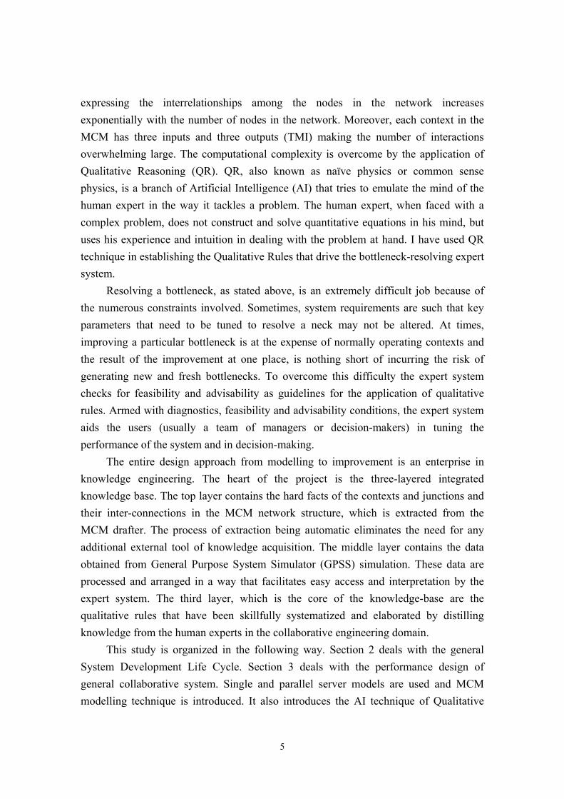
To achieve this purpose, we insert ‘modelling-performance evaluation- performance improvement’ core cycle inside the SDLC as shown in figure 1.

6

SystemModelling

PlannedSystem

PerformanceImprovement

PerformanceEvaluation

Figure 1 Core development cycle

3. Performance Improvement by Qualitative Reasoning Performance design of collaborative systems is through the application of Qualitative Reasoning (QR) technique of AI. QR, also known as common sense physics or naïve physics is reasoning based not on rigorous mathematical formulation, but on the structure and behaviour of devices and systems. Reasoning from the first principles of structure and behaviour leads us to formulate the Qualitative Rules needed to resolve bottlenecks. Performance design task is performed by an expert system. The latter is a software program that diagnoses bottlenecks in system operation and aids the user in fine-tuning the system to obtain optimum operation. QR approach and the structure and development of the expert system are discussed in this chapter.

Qualitative Reasoning (QR) research aims to develop representation and reasoning techniques that will enable a program to reason about the behaviour of physical systems, without the kind of precise quantitative information needed by conventional analysis techniques. It is an attempt to imitate reasoning of an ordinary person who solves day-to-day problems by using nothing more than ‘common sense’. For instance, when a person observes that the water level of a reservoir is quite high and it is pouring heavily, he or she immediately reasons that the reservoir is going to overflow, without knowing the intricate details of the system such as the exact water level, the rate of change of level, etc. Let’s consider another scenario: A person is confronted with a water-filled pan on a lit stove. He or she can easily predict that the lit stove will warm the water up. At some point, the water will start to boil, and eventually evaporate leaving behind a

7

charred pan if the stove is left on for a long time. To make these predictions, the person need not know the exact values of the variables involved, such as the amount of water, the temperatures of the stove and the water, or the boiling temperature. Neither does he or she need to know the exact mathematical relations among the variables. Such are the situations in which a solution is arrived at without formulating a differential equation and solving it. The ultimate goal of the AI technique of QR is to make programs reason out qualitatively, when precise numerical details of the system are not available.

4. Performance design of general collaborative service 4.1 Single and parallel server models MCM is an ingenious modelling technique developed to model the real world systems in Collaborative Engineering. MCM is a comprehensive way of representing the workflow in Collaborative Engineering (Hasegawa et al., 200). ‘Context’ as explained below, is a conceptual interface wherein the exchange of the essential ingredients of Collaborative Engineering Systems, viz. Token, Material and Information takes place. The MCM contexts correspond to single and parallel servers of the queueing theory. Token, Material and Information flow from context to context. The linking of the various contexts through arcs representing the flow of Token, Material and Information gives rise to a topology known as the Multi-Context Map (MCM).

4.2 Contexts in MCM

Collaboration necessarily implies the presence of actors (collaborators), action (task) and ‘object upon which the action is performed’. Context is a conceptual location that facilitates the process of collaboration among the collaborators. It could also symbolically represent the physical location of the collaboration activity. The left-hand Perspective of the context represents the requestor of the activity and may include person or persons, organization, equipment, etc., while the right-hand Perspective represents the performer of the activity. Context, in a word, is the combination of these two Perspectives.

8

ContextName

Left-hand Perspective

Input Token

Input Material

Resources used by the subject in the

right-hand perspective

Resources used by the subject in the

left-hand perspective

Input Information

Output Token

Output Material

Output Information

Right-hand Perspective

Figure 2 Context in MCM

We can imagine an interface sandwiched in between the two Perspectives of the

context; these two Perspectives interact to carry on collaboration by passing the ‘object upon which the action is performed’ through the interface. In the MCM terminology the object that is passed through the interface is called Material. It could be a piece of machinery, documents, persons, etc., anything from the physical world that usually has mass or weight. Material in MCM corresponds to the transactions in the domain of discrete event simulation. Associated with the Material is the Information – a set of properties of the Material. In most practical cases, Information is the documentation that accompanies the Material as the latter is processed at the context. Another important feature of the interface is that it produces Token. Token is a collection of facts which are mutually recognized and acknowledged by the two collaborating parties. Tokens can be transmitted to different contexts as telecommunication or as face-to-face communication.

The context, then, is the basic unit in collaboration work. The actors in the context are the collaborators, the action is the service that is being offered and the object that is acted upon is the Material with its accompanying Information. Finally, the Token completes the picture of the collaboration between the right-hand and the left-hand Perspectives of the context. MCM is the collective linking of contexts. The flow of Token, Material and Information (hereafter, TMI ) from context to context is governed by a set of junctions, whose properties and functions are described below. 4.3 MCM Example Real life example of a general clinic is considered to illustrate the MCM modelling

9

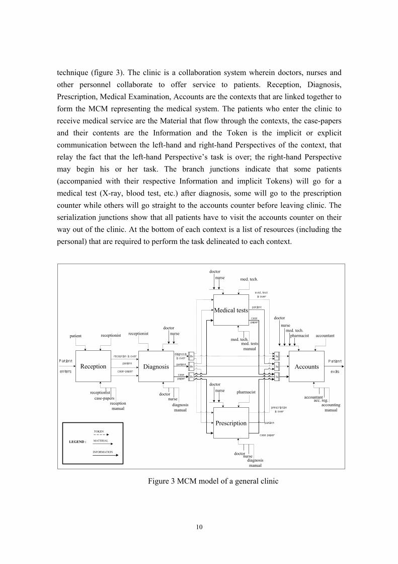
technique (figure 3). The clinic is a collaboration system wherein doctors, nurses and other personnel collaborate to offer service to patients. Reception, Diagnosis, Prescription, Medical Examination, Accounts are the contexts that are linked together to form the MCM representing the medical system. The patients who enter the clinic to receive medical service are the Material that flow through the contexts, the case-papers and their contents are the Information and the Token is the implicit or explicit communication between the left-hand and right-hand Perspectives of the context, that relay the fact that the left-hand Perspective’s task is over; the right-hand Perspective may begin his or her task. The branch junctions indicate that some patients (accompanied with their respective Information and implicit Tokens) will go for a medical test (X-ray, blood test, etc.) after diagnosis, some will go to the prescription counter while others will go straight to the accounts counter before leaving clinic. The serialization junctions show that all patients have to visit the accounts counter on their way out of the clinic. At the bottom of each context is a list of resources (including the personal) that are required to perform the task delineated to each context.

Reception

patient

receptionistcase-papers

receptionmanual

Diagnosis

receptionistdoctor

nurse

doctornurse

diagnosismanual

Accounts

med. tech.

accountantacc. reg.

accountingmanual

doctor

nurse

Prescription

nurse

doctornursediagnosismanual

doctor

pharmacist

Br

Br

Br

Medical tests

nurse

med. tech.med. tests

manual

doctor

med. tech.

Se

Se

Se

Patient

exits

Patient

enters

accountantreceptionist

reception is over

patient

case-papercasepaper

patient

diagnosisis over

med. testis over

prescriptionis over

patient

patient

case paper

casepaper

pharmacist

TOKEN

MATERIAL

INFORMATION

LEGEND :

Figure 3 MCM model of a general clinic

10

4.4 Bottlenecks in MCM MCM is a network of contexts and junctions. Junctions direct the flow of TMI through the exchange of which the contexts interact with one another. Due to the limitations on the service time of each context and due to the problems in the flow of TMI, bottlenecks can occur at the contexts and at the junctions. Conventionally, bottlenecks are locations of congestions in a network. However, we consider any situation of the context (server) that does not allow the context to be operating in its optimum range as a bottleneck. Thus, under-utilization of the context is also a bottleneck. In this section we formally define the bottlenecks that can occur at these two different locations.

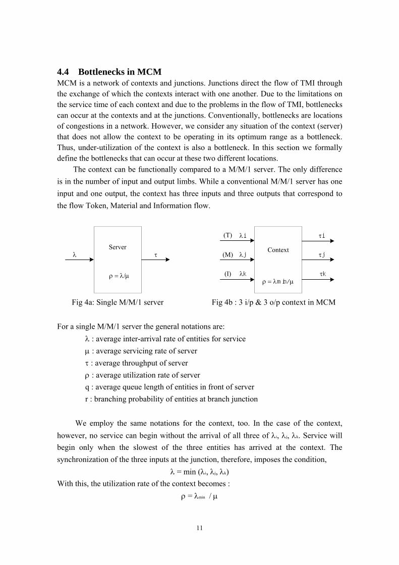
The context can be functionally compared to a M/M/1 server. The only difference is in the number of input and output limbs. While a conventional M/M/1 server has one input and one output, the context has three inputs and three outputs that correspond to the flow Token, Material and Information flow.

τλServer

ρ = λ/µ

Context

ρ = λmin/µ

λi

λj

λk

τi

τk

τj

(T)

(M)

(I)

Fig 4a: Single M/M/1 server Fig 4b : 3 i/p & 3 o/p context in MCM

For a single M/M/1 server the general notations are:

λ : average inter-arrival rate of entities for service µ : average servicing rate of server τ : average throughput of server ρ : average utilization rate of server q : average queue length of entities in front of server r : branching probability of entities at branch junction

We employ the same notations for the context, too. In the case of the context,

however, no service can begin without the arrival of all three of λi, λj, λk. Service will begin only when the slowest of the three entities has arrived at the context. The synchronization of the three inputs at the junction, therefore, imposes the condition,

λ = min (λi, λj, λk) With this, the utilization rate of the context becomes :

ρ = λmin / µ

11

This implies that with the increase in λmin or with the decrease in µ, ρ increases steadily. From expert’s heuristics (failure-to-safety aspect) ρ > 0.7 is an indication of the possibility of a bottleneck. As λ rises, in addition to rising ρ , TMI queues begin to develop in front of the contexts; i.e. T, M and I arrive independently at the context, form a TMI set and wait for service. After sufficient lapse of time, the TMI sets develop TMI queues. Q > 1.0, is another landmark indicating the possibility of bottleneck, from failure-to-safety aspect. On the other hand, ρ < 0.3 is an indicator of underflow of TMI or under-utilization of the resources in collaborative system. Finally, what distinguishes contexts in MCM from ordinary M/M/1 servers is the three-input-three-output TMI scheme. Due to lack of uniformity in the flow of TMI at a given context, a state of imbalance is created. In other words, the time-lag in the arrivals of T, M and I results in independent T-queue, M-queue and I–queue. This imbalance, in addition to overflow and underflow, is another aspect of bottleneck.

Summarizing the above measurable parameters, we formally define a bottleneck to be a context that has at least one of the following characteristics. 1. ρ is low (ρ < 0.3) 2. ρ is high (ρ > 0.7) 3. TMI imbalance (at least one of qi, qj, qk > 1.0) 4. (TMI)q is long (q > 1.0)

4.5 Resolution of Bottlenecks By analyzing the GPSS simulation data, the expert system checks for bottlenecks at the contexts and junctions and displays them to the user. When the user selects a particular bottleneck for resolving, the expert system makes extensive use of the knowledge base to draw a parameter tuning plan that will resolve the bottleneck in question. The inference engine of the expert system uses the following qualitative rules in coming to its conclusion. First it applies the context rules to the bottleneck context; but the bottleneck cannot possibly be resolved by changing the context (i.e. local) parameters; so the inference engine moves upstream and checks for junctions that may be the source of the bottleneck; it applies the junction rules; if the resolution is not achieved at this stage, then it moves on to the previous contexts, applies the rules and so on. Moreover, at each stage the inference engine determines the mini-structure in which the context is located and thereby applies the mini-structure rules. The nature of these rules and the instances of their application is discussed below.

12

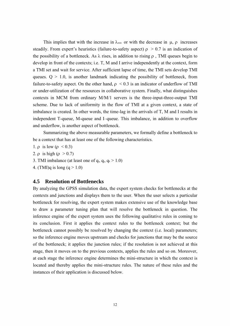
4.5.1 Knowledge-based qualitative rules The rules which control the functioning of the inference engine of the expert system are qualitative in nature. We intuitively know that the variables of a context are related by some kind of a monotonic relationship. It is natural to think, for instance, that ρ can be decreased by increasing µ or decreasing λ. Knowledge representation in the form of qualitative rules is a way of concretizing these intuitive qualitative relations (Sawamura et al., 1989). When the value of a certain parameter is found to be high, the rule simply states, “increase/decrease the controlling parameter”. Again, when the value of a certain parameter is found to be low, the rule simply states, increase/decrease the controlling parameter”. There are no quantitative calculations performed. The landmark values are sufficient to drive the inference engine. Below we group the rules into three categories depending on when and how they are applied as the expert system goes about resolving a given bottleneck. Further, by intuition we know that in the case of overflow, one input could be high, two inputs could be high or all three inputs could be high. The table below summarizes this qualitative way of thinking.

Table 1 Qualitative rules for a context in isolation (rules 1-10)

Rule

Symptom State of

Solution

qi qj qk ρ λi, λj, λk λi λj λk µ 1 1 1 1 H overflow ↓ ↓ ↓ ↑ 2 0 1 1 H overflow/imbalance ↓ ↓ ↓ ↑ 3 0 1 1 M imbalance 〇 ↓ ↓ 〇

4 0 1 1 L underflow/imbalance ↑ 〇 〇 ↓ 5 0 0 1 H overflow/imbalance ↓ ↓ ↓ ↑ 6 0 0 1 M imbalance 〇 〇 ↓ 〇

7 0 0 1 L underflow/imbalance ↑ ↑ 〇 ↓ 8 0 0 0 H overflow ↓ ↓ ↓ ↑ 9 0 0 0 M optimum flow 〇 〇 〇 〇

10 0 0 0 L underflow ↑ ↑ ↑ ↓ H: High; M: Medium; L: Low; ↓: Decrease; ↑: Increase; 〇: Do not change

Depending on the state of q and ρ, increase or decrease λ and/or µ. In this set

of rules, there are straight forward rules like Rule 1 which states that all inputs should be reduced when ρ is high; however, there are also subtle rules like Rule 4, Rule 5, etc.,

13

which state that even the low inputs have to be decreased when ρ is high.

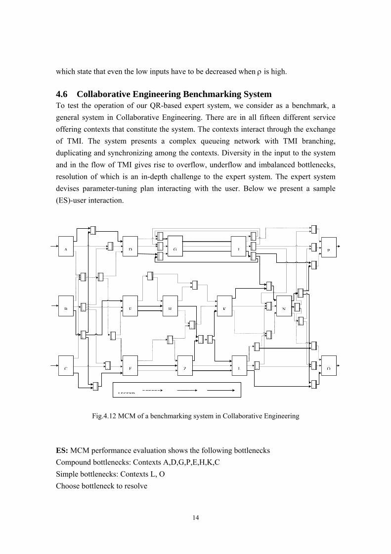
4.6 Collaborative Engineering Benchmarking System To test the operation of our QR-based expert system, we consider as a benchmark, a general system in Collaborative Engineering. There are in all fifteen different service offering contexts that constitute the system. The contexts interact through the exchange of TMI. The system presents a complex queueing network with TMI branching, duplicating and synchronizing among the contexts. Diversity in the input to the system and in the flow of TMI gives rise to overflow, underflow and imbalanced bottlenecks, resolution of which is an in-depth challenge to the expert system. The expert system devises parameter-tuning plan interacting with the user. Below we present a sample (ES)-user interaction.

D

B

C

E N

F O

G

H

Z

J

K

L

PA

B

B

S

S

S

S

B

B

B

S

S

S

S

B

D

S

B

S

S

S

S

S

S

S

B

S B

S

S

S

LEGENDTOKEN MATERIAL INFORMATION

Fig.4.12 MCM of a benchmarking system in Collaborative Engineering

ES: MCM performance evaluation shows the following bottlenecks Compound bottlenecks: Contexts A,D,G,P,E,H,K,C Simple bottlenecks: Contexts L, O Choose bottleneck to resolve

14

User Choice: Context P ES: Characteristics of bottleneck at context P are: ρ = 0.215; Tq = 0.000; Mq = 19.764; Iq = 87.685 ES: Can you increase context service time? (feasibility) User: No ES: To increase flow to context P, increase input to context B (mini-structure knowledge, rule 16). In addition this will also resolve bottleneck at contexts E,H,K due to underflow (advisability). To resolve the TMI imbalance queues, can you increase the Token flow from context N to context P? (feasibility) User: Yes ES: Here is the improvement plan – Increase M & I flow from context B to E; Increase T flow from context N to P Improved performance: Characteristics of context P after improvement ρ = 0.532 (0.3 < ρ < 0.7) Tq = 0.106; Mq = .696; Iq = 0.443 (Tq,Mq,Iq < 1.0) In addition, bottlenecks at contexts E, K & K are resolved. 5. Performance design of distributed collaborative service In collaborative systems, collaborators get together to offer a variety of services in a variety of ways. In order to evaluate and eventually improve the performance of the collaborative systems, we need to model the diverse type of services and service-offering-methods that are being used by the collaborators. The MCM model consisting of single and parallel servers discussed in Scenario 1 represents the general type of collaborative service. The composite-server model in Scenario 2, represents the composite nature of service in collaborative systems. The type of service discussed in this chapter is distributed service. This type of service that is often encountered in collaborative systems is represented by the ‘distributed service model’.

In a distributed type of service, the service-providing unit, (SPU) move from server to server in order to offer service. This situation can be neatly described by Petri nets. Petri nets are powerful graphical tools that depict the workflow in collaborative systems. In particular, they point out the inconsistencies and clashes in the system workflow. Petri nets, however, give the users great freedom and flexibility in their description and usage. This often results in a certain amount of ambiguity in the Petri net system description. Senuma et al. (2002) have devised well-disciplined Petri nets

15

for use in the description of collaborative engineering systems. In this chapter I have used well-defined Petri nets as client-server models to

represent the distributed type of service found in common collaborative systems. The use of well-defined Petri nets is further illustrated by citing practical example of a collaborative system that has widespread distributed service in it. Since the same SPU has to attend to a number of servers distributed serially, the overall performance of the SPUs tend to be loaded. A set of qualitative rules have been laid down to improve the performance of the system with distributed service. The expert system uses these rules to minimize the load and improve the overall performance of the system. 5.1 Petri nets Petri nets were first introduced by Carl Adam Petri and are named after him. They are formal, graphical techniques used for the specification and analysis of concurrent, discrete-event dynamic systems. One of the major advantages of Petri nets is that they enable to understand and express simply and naturally all problems and properties related to parallelism and concurrency (Diaz, 1987). Sometimes there are multiple independent dynamic entities within a system. Petri nets are ideal in depicting such systems which exhibit concurrency such as client-server networks, work-flows, real-time systems, distributed databases, telecommunications, etc. There are three main actors in a process control scenario, namely, the process, the control system and the process operator. The three may be seen to be acting concurrently with respect to each other. Within the process, several components of the process may evolve concurrently with respect to each other. With respect to the control system, the process is evolving concurrently. With respect to the process and the control system, the operator may concurrently be taking several decisions and actions. These different actors and the concurrency of actions can be distinctly represented by Petri nets. In addition, the graphical representation by Petri nets facilitates visualization of complex processes. 5. 2 Petri Net Model of Distributed Service In some collaborative engineering systems, a person or a group of persons have to perform a series of jobs. In the modelling language the jobs are represented by servers and the group of persons that performs tasks or offers service are known as service providing units (SPU). If the servers are serially arranged to form a queueing network, it would imply that the SPUs move from server to server by way of providing service. The service offered by SPUs is therefore a distributed type of service.

The concept of distributed service can be neatly depicted by Petri nets. The Petri

16

net shown in figure 6 portrays the client-server model. Orders for service or customers for service arrive at the entry point of the system. Places may be thought of as physical or logical locations where customers queue for service. Transitions are locations where service is being offered. SPU is depicted on the left hand side. As the SPU finishes offering service at one transition, it moves to the next transition, and so on, till the series of jobs that are assigned to it are completed.

Tr2

Tr3

Tr4

Tr5

Server

Tr1

Pl1

Pl2

Pl3

Pl4

Figure 6 Petri net client-server model

5.3 Practical Example of Collaborative Engineering System with Distributed System Figure 7 shows a practical example of distributed service. There are in all four service lines, each offering distributed service. On each line there are servers represented by black dots. S1,S4 Entry points U1,….Z1 Service line 1 U2,…Z2 Service line 2

17

U3,….Z3 Service line 3 U4,….Z4 Service line 4 P1, P2, P3, P4 Perspectives acting as servers

S1

U1

V1

W1

X1

Y1

Z1

U2

V2

W2

X2

Y2

Z2

U3

V3

W3

X3

Y3

Z3

S4

U4

V4

W4

X4

Y4

Z4

P1 P2 P3 P4

Figure 7 Collaborative system with distributed service System Operation Transactions arriving for service enter the system at transition S1 and are processed by Perspective P1 through the transitions S1, U1, V1, W1. After being processed at W1, the transactions are directed to U2 on line 2. Here the transactions are processed by P2 from transitions U2 through V2. After processing at V2, the transactions are passed on to line 3 for further processing. These transactions have to synchronize with the ones coming from transition V4 on line. Once the processing is over, the transactions on line 3 continue to be processed down the line till Y3. After passing through Y3, they are sent back to line 2 at transition W2, from where they continue to move through the line being processed at the rest of the transitions on that line.

Similar service distribution occurs along line 4. Transactions enter for service

18

through the entry port S4 and are processed till V4. They are then passed on to V3 of line 3. There they synchronize with transactions coming from line 2. They are sent back to the original line 4 after receiving service at V3 and W3 on line 2. However, once again they are sent to service line 3 from the end of which they come back to finish the rest of the processing on line 4.

5.4 Performance Evaluation If we were to allocate sufficient number of SPUs at each server in the system, the operation of the system in principle could be maintained at an optimum level. However, real-life collaborative systems have restrictions on the SPUs that can be employed due to the cost factor. Because of these restrictions imposed by the limited resources, the system operation often tends towards a rather loaded state. We select two significant parameters defined below to evaluate the performance of the system. 1. Utilization is high (ρ > 0.7) 2. Utilization is low (ρ < 0.3) 3. Queue is long (q > 1.0)

ρ > 0.7 shows that there is load on the system. It is an indication that the Perspectives acting as servers on a given line are occupied more than seventy percent of the operation time. The arrival of the transactions for service is too rapid for thePerspectives to handle; on the other hand ρ < 0.3 is a sign of the under-utilization of the system resources; the servers are idle for over seventy percent of the operation time. Q > 1.0 is an indication that the arrivals are so rapid that the servers cannot cope up with the arrival rate.

The expert system diagnoses the transitions that exhibit the above bottleneck characteristics and displays them to the user. The user then selects the bottlenecks that he or she wants the expert system to resolve. The expert system then comes up with parameter tuning plan which the user puts into effect to resolve the chosen bottlenecks. 5.5 Performance improvement The performance improvement algorithm makes use of the following principles 1. alteration of priority level 2. service-time reduction 3. increase in personnel 4. matching processing with the requests

19

These principles arise from the knowledge and heuristics of the domain expert. They are the ‘know-how’ by which the expert would try to resolve the bottlenecks in the distributed service system. The rules tabulated below represents this knowledge in a structure way.

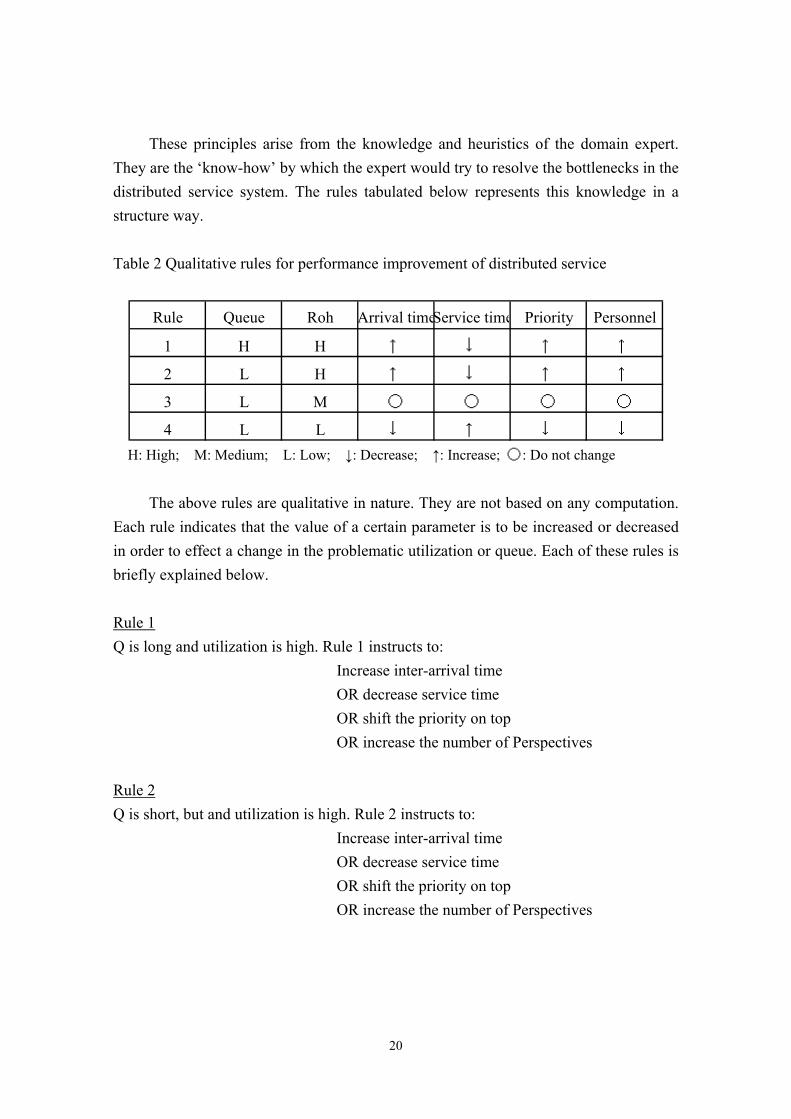
Table 2 Qualitative rules for performance improvement of distributed service

Rule Queue Roh Arrival timeService time Priority Personnel

1 H H ↑ ↓ ↑ ↑

2 L H ↑ ↓ ↑ ↑

3 L M 〇 〇 〇 〇

4 L L ↓ ↑ ↓ ↓ H: High; M: Medium; L: Low; ↓: Decrease; ↑: Increase; 〇: Do not change

The above rules are qualitative in nature. They are not based on any computation.

Each rule indicates that the value of a certain parameter is to be increased or decreased in order to effect a change in the problematic utilization or queue. Each of these rules is briefly explained below. Rule 1 Q is long and utilization is high. Rule 1 instructs to: Increase inter-arrival time OR decrease service time OR shift the priority on top OR increase the number of Perspectives Rule 2 Q is short, but and utilization is high. Rule 2 instructs to: Increase inter-arrival time OR decrease service time OR shift the priority on top OR increase the number of Perspectives

20

Rule 3 Q is short and utilization is medium. Rule 3 instructs: Not to change the inter-arrival time AND not to change service time AND not to change priority AND not to change the number of Perspectives Rule 4 Q is short and utilization is low. Rule 3 instructs to: Decrease inter-arrival time OR increase service time OR shift the priority lower OR decrease the number of Perspectives Table 3 Performance evaluation and improvement of practical system

Transi- State before Improvement State after Improvementtion Performance

Arrival Service Arrival ServiceTime Time Priority P(count) q roh Time Time Priority P(count) q ro

S1 11,3 3 ** ** ** 11,3 3 ** ** **U1 9 1 (P1) 0.2 0.81 9 1 (P1) 0.2 0.81V1 11 2 9.2 0.88 7.5 2 0.4 0.62W1 3 3 2 42.2 0.13 3 3 2 42.2 0.13X1 10 4 35.8,13.2 0.01 10 4 35.8,13.2 0.01Y1 3 5 0 0.01 3 5 0 0.01Z1 12 6 0.4 0.02 12 6 0.4 0.02U2 3 1 (P2) 0.2 0.11 3 1 (P2) 0.2 0.11V2 5 2 0 0.18 5 2 0 0.18W2 7 3 2 21.8,0 0.1 7 3 2 21.8,0 0.1X2 6 4 0.8 0.09 6 4 0.8 0.09Y2 8 5 0.2 0.11 8 5 0.2 0.11Z2 13 6 0 0.19 13 6 0 0.19U3 5 1 (P3) 0.4 0.18 5 1 (P3) 0.4 0.18V3 8 2 0,46.6 0.29 8 2 0,46.6 0.29W3 15 3 2 2.6 0.6 15 3 2 2.6 0.6X3 9 4 17.2,2.6 0.13 9 4 17.2,2.6 0.13Y3 3 5 0.8 0.04 3 5 0.8 0.04Z3 4 6 0 0.07 4 6 0 0.07S4 12,4 11 ** ** ** 12,4 11 ** ** **U4 5 1 (P4) 0 0.4 5 1 (P4) 0 0.4V4 7 2 0.6 0.51 7 2 0.6 0.51W4 14 3 2 55.8,6.2 0.39 14 3 2 55.8,6.2 0.39X4 8 4 7.8 0.14 8 4 7.8 0.14Y4 10 5 6.6,2.4 0.13 10 5 6.6,2.4 0.13Z4 2 6 1.6 0.02 2 6 1.6 0.02

Performance Given Parameters Altered Parameters

h

21

The result of Petri net simulation is shown in table 3. On analyzing the performance data in the above table we find that the utilization of several transitions is low (ρ < 0.3), for some it is high, (ρ > 0.7) and still for some the queue length is large (q > 1.0). Transition V1 is the most server bottleneck, (ρ = 0.8776; q = 9.2). After carrying on the performance diagnosis, the expert system displays a list of bottlenecks to the user. The user chooses one or more bottlenecks for resolving. In the given example, the user chooses transition V1 for performance improvement. It is the judgment of the expert system, that the value of the service time parameter of transition V1 should be decreased to improve the performance. The expert system also judges that changing this particular parameter does not adversely affect the operation of any of the transitions in the entire system. The user follows the instructions of the expert system and reruns the simulation to get the improved operation of transition V1. Further, since the approach in resolving bottlenecks is qualitative, the expert system does not give an estimate of the amount of decrease the user should make in the service time; the only general instruction issued is that the decrease should not be too rapid and too large, to avoid leaving a bad impact on the entire system. The user carries on the performance improvement task in several steps which are listed in the table 4. Step zero is the original state of the system before being instructed to improve. Steps 1-16 show the gradual decrement in service time that leads to the performance improvement of transition V1. The final steps show an improvement not only in utilization of the transition, but also a drastic reduction in the queue length. This improvement is beneficial to the servers as well as to the customers. Reduction in utilization means the free time of the servers has relatively increased and the reduction in queue-lengths means that the customers do not have to spend time in queueing for service. These two results are shown by the two graphs that follow.

22

Table 4 Step-wise performance improvement

Step no. Service-time Queue-length Utilization0 11 9.2 0.8775711 10.75 9.4 0.8219592912 10.5 7.4 0.82883483 10.25 5.6 0.5567107784 10 2.8 0.8797656885 9.75 5.6 0.5567107786 9.5 2.8 0.7446342077 9.25 5.8 0.8457463168 9 3.6 0.8600950699 8.75 4.2 0.76392182

10 8.5 2 0.79094910911 8.25 0.6 0.77213409812 8 0.2 0.73875739413 7.75 3 0.70293871914 7.5 0.4 0.61688718915 7.25 0.8 0.689141182

0

0.1

0.2

0.3

0.4

0.5

0.6

0.7

0.8

0.9

1

1 2 3 4 5 6 7 8 9 10

utilization

Graph 1 Utilization improvement in transition V1.

23

0

1

2

3

4

5

6

7

8

9

10

1 2 3 4 5 6 7 8 9 10 11 12 13

queue-length

Graph 2 Queueing improvement in transition V1.

6. Conclusion When planning and designing systems, the operational aspect, in many cases, is not taken into consideration. System operation testing, if it is done, takes place only after the implementation phase of the system development life cycle. However, it is too difficult to make changes in the system that is already implemented. The number of changes possible is limited and with every element that is changed, the cost rises steadily. Contrary to this reactive approach of resolving system operational problems when they are discovered, a predictive approach of foreseeing system operational problems and suggesting operational improvement is proposed in this study. The strategy is to estimate system performance and outline improvement directives at the requirement analysis and design phases, much before the implementation phase.

The three phases of system modelling, performance evaluation and performance improvement form the core life cycle, which can be embedded in the normal life cycle of system development. In this study, novel tools for modelling, performance evaluation and performance improvement are introduced. Modelling is done by the Multi-Context Map (MCM) technique, performance evaluation is by GPSS simulation and improve- ment is by Expert System reasoning with Qualitative rules. Token, Material and Information (TMI) are the three types of flows identified by the MCM modelling

24

methodology. qualitative Reasoning is applied to overcome the mathematical complexity resulting from the three-way interactions among the MCM contexts.

The target systems of analysis and design are collaborative systems. The subsystems that make up a collaborative system collaborate with each other to offer service to the clients that enter the system. Collaboration at three different levels, namely, inter-collaboration, intra-collaboration and micro-collaboration have been considered in this study. In addition, three distinct scenarios of collaborative activity are examined in detail. At the centre of each scenario is a server-model that is being developed to represent a particular type of service in collaborative systems.

In scenario 1, single and parallel servers model the general type of collaborative activity. These server models are well-known mathematical expressions in the waiting line analysis (also known as queueing theory) of Operations Research. The system operation simulation data obtained from GPSS simulation is referred to by the expert system and analyzed for bottlenecks. For every bottleneck chosen by the user for resolving, the expert system draws a parameter tuning plan. Parameter tuning is done locally, while taking into consideration the propagation of effects globally. This performance design approach is rigorously tested on the general collaborative engineering system benchmark in scenario 1. It is found to be effective in improving the bottlenecks that appear in the operation of the collaborative engineering system benchmark.

In scenario 2, distributed service in collaborative systems is analyzed. The well-disciplined version of Petri nets is a natural choice for modelling distributed type of service. The problems of simultaneity, concurrency and clash are readily brought to light by the Petri net visualizer. In addition, the non-visual operational problems, as in scenarios 1 and 2, are discovered by the performance evaluating program. Finally, the bottleneck resolving expert system driven by qualitative rules is once again found to achieve the improvement task in the case of the practical system with distributed service dealt with in scenario 3.

Each of the above three stages of the core life cycle has a suite of implementation tools. Microsoft Visio is used for drafting MCM, Minuteman Software’s GPSS World is used for developing performance evaluating program and Logic Programming Associates’ Flex is used to build the bottlenecks diagnosing and performance improving expert system. Further, this study has also proposed an integrated environment for the implementation of the above three phases of the core life cycle. The development of each phase, directly leads into the next phase. This is made possible by the intermediate conversion tools that link the three phases. The integrated environment of model

25

building, performance evaluation and performance improvement is semi-automatic by design, and as demonstrated by the successful application to the performance design and improvement of the benchmarking systems, can be extended to real life collaborative engineering systems.

7. References Anderson, D. R.; Sweeney, D. J.;, and Williams, T. A. 2003. An Introduction to Management Science, Quantitative Approaches to Decision Making. South-Western, Ohio, tenth edition. Banks, J., and Carson II, J.S. 1984. Discrete-Event System Simulation. Prentice-Hall, Inc., Englewood Cliffs, New Jersey. Bratko, I. 2001. Prolog Programming for Artificial Intelligence. Addison Wesley, London, third edition. Cooling, J., 2003. Software Engineering for Real-time Systems, Addison-Wesley. Davies, R. 1985. Qualitative Reasoning about Physical Systems. In Bobrow, D.G. editor 1985, Qualitative Reasoning about Physical Systems. MIT Press, Cambridge, MA, 347-410. de Kleer, J., and Forbus, K. D. 1993. Building problem solvers. MIT Press, Cambridge, MA. de Kleer, J. 1985. How Circuits Work. In Bobrow, D.G. editor 1985, Qualitative Reasoning about Physical Systems. MIT Press, Cambridge, MA, 205-280. Diaz, M. 1987. Applying Petri Net Based Models in the Design of Systems. In Voss, K.; Genrich, H.J.;, and Rozenberg, G. editors 1987, Concurrency and Nets: Advances in Petri Nets, Springer-Verlag, Berlin, 23-67. Finlay, J., and Dix, A. 1996. An introduction to Artificial Intelligence. Routledge, London. Fishman, G. S. 1978. Principles of Discrete Event Simulation. John Wiley & Sons, New York.

26

Gordon, G. 1975. The Application of GPSS V to Discrete System Simulation, Prentice-Hall, Inc., Englewood Cliffs. New Jersey. Hasegawa, A.; Kumagai, S.;, and Itoh K. 2000. Collaboration Task Analysis by Identifying Multi-Context and Collaborative Linkage. CERA 8(1):61-71. Hellerstein, J. 1992. Obtaining Quantitative Estimates from Monotone Relationships. In Faltings, B., and Struss, P., editors 1992, Recent Advances in Qualitative Physics. MIT Press, Cambridge, MA 360-374. Hoffer, J. A.; George, J. F.;, and Valacich, J. S. 2002. Modern System Analysis & Design. Prentice-Hall International, Inc., third edition. Itoh K.; Honiden, S.; Sawamura, J.;, and Shida, K. 1990. A Method for Diagnosis and Improvement on Bottleneck of Queuing Network by Qualitative and Quantitative Reasoning. Journal of Artificial Intelligence (Japanese) 5(1):92-105. Itoh K.; Hirota T.; Okabe, M.;, and Kawabata R. 2003. Foundation of Information System’s Technology (Japanese). Kyoritsu, Tokyo. Kiriyama, T.; Kurumatani K.; Tomiyama T.;, and Yoshikawa H. 1989. Qualitative Behavior Representation and Reasoning for Intelligent CAD Systems. In Kimura, F., and Rolstadas A., editors 1989, Computer Applications in Production and Engineering. Elsevier Science Publishers B.V., Amsterdam. 29-36. Karian, Z. A., and Dudewicz, E. J. 1999. Modern Statistical, Systems, and GPSS Simulation. CRC Press, London, second edition. Klienrock, L. 1975. Queuing Systems, John Wiley & Sons, Inc.. Kuipers, J. 1994. Qualitative Reasoning Modeling and Simulation with Incomplete Knowledge. MIT Press, Cambridge, MA. Lazowska, E.D.; Zahorjan, J.; Graham, G. S.;, and Sevcik, K. C. 1984. Quantitative System Performance Computer System Analysis Using Queueing Network Models. Prentice-Hall, Inc., Englewood Cliffs, New Jersey.

27

Liu, Z.Y., and Farley, A.M. 1991. Structural Aggregation in Commonsense Reasoning. Proceedings of the National Conference on Artificial Intelligence AAAI-91:868-873. Martin, J. 1989. Information Engineering, Book I. Englewood Cliffs, Prentice Hall. Minsky, M. 1975. A framework for representing knowledge. In Windton, P.H., editor 1975, The psychology of computer vision. McGraw-Hill, New York. Nikolopoulos, C. 1997. Expert Systems: Introduction to First and Second Generation and Hybrid Knowledge Based Systems. Marcel Dekker Inc., New York. Oliver, W.O.; Kelliher, T.P.;, and Keegan Jr., J.G. 1997. Engineering Complex Systems with Models and Objects. McGraw-Hill, New York. Ross, S. M. 1990. A Course in Simulation. Macmillan Publishing Company, New York. Sawamura, J.; Shida, K.; Honiden, S.;, and Itoh, K. 1989. Bottleneck Diagnosis for Queuing Network using Knowledge Engineering. Journal of Information Processing (Japanese) 30(8):990-1002. Senuma, Y.; Maruyama, J.; Kwabata, R.;, and Itoh, K. 2002. Effective Use of Model Diagrams in System Analysis. FOSE 9:61-71. Shannon, R. E. 1975. System Simulation: The Art and Science. Prentice-Hall, Englewood Cliffs, New Jersey. Shelly, G. B.; Cashman, T. J.;, and Rosenblatt, H., J. 2003. System Analysis and Design. Course Technology, Boston, fifth edition. Whitehouse, G. E., and Wechsler, B.L. 1976. Applied Operations Research: A Survey. John Wiley & Sons, New York. Williams, B. K., and Sawyer, S. C. 2003. Using Information Technology: A Practical Introduction to Computers & Communications. McGraw-Hill/Irwin, New York, fifth edition.

28