Embed Size (px)
Citation preview
Journal of Computational Physics 201 (2004) 685–722
www.elsevier.com/locate/jcp
A surfactant-conserving volume-of-fluid method forinterfacial flows with insoluble surfactant
Ashley J. James a,*, John Lowengrub b
a Department of Aerospace Engineering and Mechanics, University of Minnesota, 107 Akerman Hall, 110 Union St SE,
Minneapolis 55455, USAb Department of Mathematics, University of California, Irvine
Received 1 March 2004; received in revised form 15 June 2004; accepted 23 June 2004
Available online 13 August 2004
Abstract
An axisymmetric numerical method to simulate the dynamics of insoluble surfactant on a moving liquid–fluid inter-
face is presented. The motion of the interface is captured using a volume-of-fluid method. Surface tension, which can be
a linear or nonlinear function of surfactant concentration (equation of state), is included as a continuum surface force.
The surfactant evolution is governed by a convection–diffusion equation with a source term that accounts for stretching
of the interface. In the numerical method, the masses of the flow components and the surfactant mass are exactly con-
served. A number of test cases are presented to validate the algorithm. Simulations of a drop in extensional flow, and its
subsequent retraction and breakup upon cessation of the external flow, are performed. Even when the initial surfactant
distribution is dilute, we observe that increases in surfactant concentration locally (i.e. at the drop tips) can result in a
local deviation from the dilute limit. We show that this can lead to differences in effective surface tension, the Marang-
oni forces and the associated drop dynamics between results using the linear and nonlinear equations of state.
� 2004 Elsevier Inc. All rights reserved.
Keywords: Surfactant; VOF; Interfacial flow; Surface tension
1. Introduction
Surfactant plays a critical role in numerous important industrial and biomedical applications. For exam-
ple, the formation of very small drops or bubbles by tip streaming relies on the presence of surfactant [1].
The production of such tiny droplets is useful in drug delivery, industrial emulsification [2], liquid/liquid
0021-9991/$ - see front matter � 2004 Elsevier Inc. All rights reserved.
doi:10.1016/j.jcp.2004.06.013
* Corresponding author. Tel.: +1-612-625-6027; fax: +1-612-626-1558.
E-mail addresses: [email protected] (A.J. James), [email protected] (J. Lowengrub).
686 A.J. James, J. Lowengrub / Journal of Computational Physics 201 (2004) 685–722
extraction and hydrodesulfurization of crude oil [3], polymer blending and plastic production [4], and other
applications.
Surfactants adhere to interfaces resulting in a lowered, non-uniform surface tension along the interface.
This makes the capillary force non-uniform and introduces the Marangoni force. Further, there may be
exchange (adsorption/desorption) of surfactants between the interface and the bulk [2]. Interfacial surfac-tant is transported with the interface by convection, and may diffuse along the interface in the presence of a
surfactant concentration gradient. Additionally, compression or stretching of the interface causes a corre-
sponding increase or decrease in the concentration. The equation that governs these dynamics has been de-
rived in various forms in [5,6] and is derived in Appendix A in an alternate form that we use here. The
motion of the surfactant and of the surrounding bulk fluids are coupled through the Marangoni force.
While there have been many numerical studies of clean, deformable interfaces, there have been few stud-
ies that incorporate the effects of surfactants. In axisymmetric Stokes flows, Stone and Leal [7] investigated
the effect of insoluble surfactant on drop-breakup. Milliken et al. [8] investigated the effects of the drop/ma-trix viscosity ratio and the nonlinear equation of state relating the surface tension to the surfactant concen-
tration. Pawar and Stebe [9] investigated the effects of interfacial saturation and interaction. Eggleton et al.
[10] further investigated the effect of the nonlinear equation of state and finally Eggleton et al. [11] used
boundary integral methods to investigate the onset of tip streaming. In fully 3D flows, Li and Pozrikidis
[12] and Yon and Pozrikidis [13] investigated the effects of insoluble surfactant on drop dynamics in Stokes
flows using boundary integral methods. Solubility effects were considered in Stokes flows by Milliken and
Leal [14] for axisymmetric drop dynamics and very recently by Zhou et al. [15] for drop–drop interactions
and coalescence in 3D. The latter work utilized a sharp-interface finite element approach.Continuum formulations of the governing sharp interface equations have been implemented numerically
primarily for clean drops although there has been recent work on surfactants by Jan and Tryggvason [16]
who studied the effect of surfactants on rising bubbles using an immersed boundary/front tracking method
and Ceniceros [17] who used a hybrid level-set/front tracking method to study the effect of surfactants on
capillary waves. Xu and Zhao [52] presented a methodology to simulate surfactant transport on a deform-
able interface in conjunction with a level set method. They did not couple their method to a flow solver, but
presented several test cases in which a velocity field is prescribed (they reported up to 6% loss of total surf-
actant mass). Very recently, Renardy and co-workers [34,51] presented simulations of 3D drops with surf-actant using the volume-of-fluid method (described further below). This work thus far has been limited to
assuming a linear relation between the surfactant concentration and surface tension (equation of state). In
our method, we allow an arbitrary equation of state.
Continuum approaches to simulating interface dynamics include immersed-boundary/ front-tracking
(e.g. see [18–22]), level set (e.g. [23–25]), phase-field (e.g. [28–33]), volume-of-fluid (VOF) (e.g. [34–
42,55,56]), coupled level-set and volume of fluid [43–45], immersed interface (e.g. see [48,49,26,27]) and
ghost-fluid (e.g. [46,47]) methods. In the latter two methods, the interface jump conditions are handled
explicitly by modifying the difference stencils near the interface in various ways. In all of the other methods,the flow discontinuities (density, viscosity) are smoothed and the surface tension force is distributed over a
thin layer near the interface to become a volume force. As the thickness of the layer approaches zero the
volume force approaches the proper surface force. The Navier–Stokes equations are then solved on a fixed
Eulerian mesh making the extension to 3D straightforward. Each method differs in the details of how this is
carried out.
The volume of fluid (VOF) method was developed by [42] and [55] and is the method we use in this pa-
per. The main advantages of the method are that the interface shape is not constrained, changes in topology
are handled automatically, and mass of each flow component is conserved exactly. The interface location iscaptured as it moves through the grid by tracking the local volume fraction. The volume fraction is con-
stant in each fluid and discontinuous at the interface. The volume fraction convection equation is solved
in every cell, but is nontrivial only near an interface. To maintain the discontinuous nature of the volume
A.J. James, J. Lowengrub / Journal of Computational Physics 201 (2004) 685–722 687
fraction care is taken not to introduce numerical diffusion when solving the equation. Numerical diffusion
would cause smoothing of the discontinuity and the interface would become smeared normal to itself. The
approach used to avoid this is to calculate the flux of one of the fluids across each cell face using a recon-
struction of the interface position. The fluxes are then used to update the volume fraction to the next time
step.As mentioned previously, Renardy et al. [34] have recently developed a VOF method for 3D drop defor-
mation in the presence of insoluble surfactants. To our knowledge, this was the first application of a con-
tinuum-based method to study surfactant dynamics. We note that tangential surface forces due to variable
surface tension had also previously been implemented in a 2D VOF method for temperature gradient dri-
ven Marangoni convection in a cavity [50]. The implementation of surfactant in [34] was somewhat ad hoc
and only surfactants with linear equations of state were considered. This method was applied to study drop
deformation in shear flows in 3D. It was found that when the drop becomes cusp-like, the simulation be-
comes sensitive to the discretization parameters and the surfactant can diffuse off the drop surface.Although the simulations appear to show tip streaming, the surfactant concentration becomes very high
at the drop tips and the surface tension actually becomes negative. A mesh refinement study indicated that
the results depend on the temporal and spatial step sizes. More recently, Drumright-Clarke and Renardy
[51] used this algorithm to examine the effect of surfactant on the critical conditions for 3D drop break-up
in shear flow.
In the current paper we present a numerical method that incorporates surfactant dynamics in an axisym-
metric, incompressible Navier–Stokes solver based on the VOF method for interface capturing. We focus
on the case of insoluble surfactant and the surfactant mass is exactly conserved along the interface by ouralgorithm. An arbitrary equation of state relating the surfactant concentration to the surface tension may
be used. A number of test cases are presented to validate the algorithm. Simulations of a drop in extensional
flow, and its subsequent retraction and breakup upon cessation of the external flow, are performed. Even
when the initial surfactant distribution is dilute, we observe that increases in surfactant concentration lo-
cally (i.e. at the drop tips) can result in a local deviation from the dilute limit. We show that this can lead
to differences in effective surface tension, Marangoni forces and the associated drop dynamics between re-
sults using the linear and nonlinear equations of state.
The remainder of this paper is organized as follows. In Section 2 we present the governing equations. InSection 3 we describe the numerical method used for the interface evolution, the surfactant evolution and
the surface tension force. In Section 4 we present a series of simulations used to validate the numerical
method. Section 5 is dedicated to conclusions and future work.
2. Governing equations
We assume that the flow is incompressible in both fluids, so the velocity, u, is divergence free, $ Æu = 0.The volume of fluid (VOF) method is used to track the interface between the two fluids, called fluid 1 and
fluid 2. In this method a volume fraction, F, is defined in each grid cell as the fraction of the cell that con-
tains fluid 1. Here we assume that F = 1 in the region interior to the interface. The volume fraction evolu-
tion is governed by a convection equation that ensures the interface moves with the velocity of the fluid
oFot
þ u � rF ¼ 0: ð1Þ
Surface tension is included via the continuum surface force (CSF) method (e.g. [54]). The CSF is included in
the momentum equation, so the momentum equation satisfies the stress balance boundary condition on the
interface. The surface tension force is calculated in every cell, but it is nonzero only near the interface.
Using the VOF and CSF methods makes it unnecessary to apply boundary conditions at the interface
688 A.J. James, J. Lowengrub / Journal of Computational Physics 201 (2004) 685–722
and one set of governing equations applies to the entire domain (cells containing only fluid 1, cell contain-
ing only fluid 2, and cells containing an interface). Since the same equations are solved in the whole domain
the density and viscosity must be retained as variables in the momentum equation even though they are
both constant in each fluid. In interfacial cells the density and viscosity are computed as linear functions
of the volume fraction. The equations are non-dimensionalized with length scale L, velocity scale U, inertialtime and pressure scales, and surface tension scale req, which is the equilibrium surface tension (the surface
tension corresponding to a uniformly distributed surfactant with equilibrium concentration Ceq). The den-
sity and viscosity are scaled by the properties of fluid 1 and for simplicity we assume graviational forces are
negligible. Thus, the momentum equation becomes
qouot
þ u � ru� �
¼ �rp þ 1
Rer � ½lðruþruTÞ� þ 1
ReCaF S; ð2Þ
where q is the density, p is the pressure, Re = q1U L/l1 is the Reynolds number, l is the viscosity and
Ca = Ul1/req is the capillary number. The surface force FS is
F S ¼ r � ½rðI � nnÞdR� ¼ �rjdRnþoros
dRs; ð3Þ
where r is the surface tension, n is the unit vector normal (outward) to the interface, dR is the surface delta
function, j is the interface curvature and s is the unit vector tangent to the interface in the s direction. The
first term on the right-hand side of Eq. (3) is the capillary force and the second term is the Marangoniforce.Additionally a density ratio, a = q1/q2, and a viscosity ratio, k = l1/l2, are defined. The normal vector
and the surface delta function are determined from the gradient of the volume fraction,
n ¼ � rFjrF j ; dR ¼ jrF j: ð4Þ
The surfactant concentration evolution is governed by a convection–diffusion equation with a source term
to account for interfacial stretching,
oCot
þ u � rC ¼ 1
PeSr2
SCþ Cn � ru � n; ð5Þ
where C is the interfacial surfactant concentration, scaled by the equilibrium concentration, Ceq, PeS = UL/
DS is the surface Peclet number, DS is the surface diffusivity of surfactant, and r2S is the surface Laplacian
operator. To see that Eq. (5) is well defined and is equivalent to alternative formulations of the surfactantequation (e.g. [5,6]), see Appendix A.
In our finite volume method, we do not solve Eq. (5) directly and instead relate the surfactant concen-
tration (in a finite volume) to the ratio of the surfactant mass M and surface area A in that volume, i.e.
C ¼ MA: ð6Þ
The surfactant mass and surface area are tracked independently as described below.
The area has been non-dimensionalized by L2 and the mass by CeqL2. Siegel [63] has also proposed
decomposing concentration into mass and area. The equations for M and A are derived as follows. The
interfacial area in a finite volume, V, is obtained by integrating the surface delta function over the volume
A ¼ZV
dR dV : ð7Þ
Integrating the concentration times the surface delta function over the volume yields the surfactant
mass,
A.J. James, J. Lowengrub / Journal of Computational Physics 201 (2004) 685–722 689
M ¼ZV
CdR dV : ð8Þ
Differentiation of Eq. (7) with respect to time yields
DADt
¼ �ZV
ðn � ru � nÞdR dV : ð9Þ
The left-hand side of Eq. (9) is the time rate of change of the area of a material element of the interface. The
right-hand side represents changes in interfacial area due to stretching. For a vanishing volume, this can be
written in differential form as
DADt
¼ oAot
þ u � rA ¼ �Aðn � ru � nÞ; ð10Þ
which is also derived by Batchelor [53]. The mass of surfactant on a material element of the interface can
change if there is diffusion along the interface. Diffusion of mass through the boundary of a finite volume
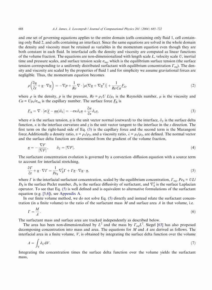
occurs through the curve where the interface intersects the boundary. A segment of this curve, called C, is
illustrated in Fig. 1. Using Fick�s Law of mass diffusion, the mass is governed by
DMDt
¼ 1
PeS
ZC
n� nV � nð Þ � rSCdC; ð11Þ
where nV is the unit vector pointed normally outward to the boundary of the volume. The cross productn� nV gives the direction tangent to both the interface and the cell, along C. Mass diffused in this direction
along the interface does not cross the boundary of the finite volume. The cross product n� nV � n gives the
other portion of the diffusion that is tangent to the interface and that does cross the boundary of the vol-
ume. Thus, the right-hand side of Eq. (11) is obtained.
Using the divergence theorem, Eq. (11) can be written as
DMDt
¼ 1
PeS
ZV
r2SCdR dV : ð12Þ
nnn V ×× ˆ
Vnn ˆ×
Volume
boundary
Interface
n
VnC
Fig. 1. Interface geometry used in evaluating interfacial diffusion of surfactant mass.
690 A.J. James, J. Lowengrub / Journal of Computational Physics 201 (2004) 685–722
This leads to a differential form for a vanishing volume
DMDt
¼ oMot
þ u � rM ¼ APeS
r2SC: ð13Þ
Eq. (5) is regained by combining Eqs. (6), (10) and (13).
Finally, an equation of state is given for the surface tension as a function of surfactant concentration. In
this method the equation of state may be linear or nonlinear. For example, the Langmuir equation of state
is
r ¼ 1þ E lnð1� xCÞ1þ E lnð1� xÞ ; ð14Þ
where E is the surfactant elasticity and x = Ceq/C* is a measure of surfactant coverage; C* is the concentra-
tion of the surfactant in the maximum packing limit. A linear equation of state can also be used:
r ¼ 1þ bð1� CÞ; ð15Þ
where b = Ex in the limit of small x. Note that for both equations of state the scaling is constructed so thatthe equilibrium dimensionless concentration, C = 1, corresponds to the equilibrium dimensionless surface
tension, r = 1.
3. Computational method
3.1. Introduction
The axisymmetric governing equations are discretized using a finite-volume method, on a fixed, struc-
tured, uniform, staggered grid, in a rectangular domain in the r–z plane. In the staggered grid arrangement
all variables except the velocity components are defined at cell centers (i, j), where index i represents a grid
line of constant r and index j represents a grid line of constant z. The radial velocity component, u, is de-
fined on ðiþ 12; jÞ cell faces and the vertical component, v, on ði; jþ 1
2Þ cell faces.
An explicit Euler time integration method is used, except that surfactant diffusion is discretized implicitlyas described in Section 3.6. At each time step, first the velocity and pressure are updated, and then the vol-
ume fraction and the surfactant distribution are updated as described below. Adaptive time stepping is used
to ensure computational stability. The time step is limited at each step by convective, viscous, and capillary
criteria. These limits are parameterized by a Courant number, DtC, a von Neumann number, DtvN, and a
capillary time step limit, DtCap, such that
Dt ¼ minDtCDxUmax
;DtvNReDx2
� �2
;DtCapReCaDx3=2 !
; ð16Þ
where Dx is the minimum spatial step size and Umax is the maximum velocity component magnitude in the
domain. In the results presented in Section 4, DtC = DtvN = DtCap = 0.1 unless otherwise specified.
Because of the convection routine used, the Courant number must be less than one to ensure that the
interface does not move through more than one grid cell in a single time step. We use 0.1 as a more con-servative value to ensure accuracy and stability. The use of other advection algorithms [67,68] could be used
to relax this time step stability constraint.
The continuity and momentum equations are discretized using second-order central differences, except
for the surface stress, which is described in Section 3.7. The explicit MAC method [57] is used to compute
the velocity and pressure fields. The resulting discrete pressure-Poisson equation is solved using an incom-
A.J. James, J. Lowengrub / Journal of Computational Physics 201 (2004) 685–722 691
plete-Cholesky conjugate-gradient method [58]. The flow solver and the volume fraction evolution algo-
rithms, and their verification, are described in more detail in [35,59].
3.2. Basic strategy for surfactant evolution
The method used to compute the evolution of the surfactant is inspired by the VOF method. In the VOF
method, the volume of fluid 1 in a grid cell at the beginning of a time step is simply the cell volume times the
volume fraction, by definition. During a time step the volume of fluid 1 that moves between each pair of
adjacent grid cells (the volume flux) is computed. The volume fraction at the end of a time step is then com-
puted as the initial volume of fluid 1 minus the net volume flux out of the cell, divided by the cell volume.
Thus, although Eq. (1) governs the evolution of the volume fraction, the method actually tracks fluid vol-
umes. This is equivalent to tracking fluid masses, since the density of each fluid is constant, and ensures
mass conservation.The surfactant concentration is the mass concentration of surfactant on the interface, just as the vol-
ume fraction is the volume concentration of fluid 1 in a grid cell. The current approach to surfactant
concentration evolution is analogous to volume fraction evolution in that surfactant mass is tracked.
The concentration in a grid cell is then determined by dividing the surfactant mass in the cell by
the surface area of the interface in the cell. Compared to the volume fraction evolution, the surfactant
concentration evolution is complicated by the fact that surfactant mass may be transported between
cells by diffusion as well as convection, and that the surface area in a cell may vary, unlike the cell
volume. Because of this, it is critical to accurately track the surface area, as well as the volume fraction.The importance of ‘‘accuracy in the representation of the surface geometry’’ has also been recognized
by Yon and Pozrikidis [13].
Thus, the concentration of surfactant in a grid cell can change by three mechanisms, as described by the
governing equation: convection, diffusion and area stretching/compression. In practice, this is accomplished
in three sub-steps during each time step. Surfactant mass and area are numerically convected in tandem
with the volume fraction, since these quantities are physically convected together. Area stretching and mass
diffusion are computed separately.
In the VOF method the interface is ‘‘reconstructed’’ at the beginning of a time step for more accuratesimulation of its evolution. This reconstruction is the approximation of the interface as a line segment in
each interfacial cell. This segment then defines where the volume of fluid 1 lies within the cell. Similarly,
to accurately describe the surfactant distribution in a grid cell the concentration is reconstructed as a linear
function along the interfacial line segment.
In the remainder of this section is organized as follows. The volume fraction and concentration recon-
structions are described first, in Section 3.3, since they are used in computing the evolution. Next, the meth-
od used to evolve the volume fraction is reviewed in Section 3.4. Then the surface area evolution is
described, Section 3.5, followed by the surfactant evolution, Section 3.6. Finally, the method used to com-pute the surface force is presented in Section 3.7.
3.3. Volume fraction and surfactant concentration reconstruction
To convect volumes of fluid while preventing smearing of the interface normal to itself it is first necessary
to reconstruct the interface from the volume fraction field. This interface reconstruction locates where the
volume of fluid 1 resides in the cell, rather than assuming both fluids are distributed uniformly. We have
found that convection of surfactant similarly suffers from excessive numerical diffusion if the surfactantis assumed to uniformly distributed along the interface, so its distribution is also reconstructed. The recon-
struction is illustrated in Fig. 2. The interface and the concentration are both reconstructed at the beginning
of each time step and at intermediate steps as needed.
Interface
Fluid 1
Fluid 2
r
z
z = ar + b
srmin
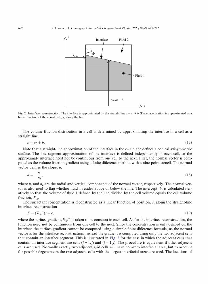
Fig. 2. Interface reconstruction. The interface is approximated by the straight line z = ar + b. The concentration is approximated as a
linear function of the coordinate, s, along the line.
692 A.J. James, J. Lowengrub / Journal of Computational Physics 201 (2004) 685–722
The volume fraction distribution in a cell is determined by approximating the interface in a cell as a
straight line
z ¼ ar þ b: ð17Þ
Note that a straight-line approximation of the interface in the r�z plane defines a conical axisymmetricsurface. The line segment approximation of the interface is defined independently in each cell, so the
approximate interface need not be continuous from one cell to the next. First, the normal vector is com-puted as the volume fraction gradient using a finite difference method with a nine-point stencil. The normal
vector defines the slope, a,
a ¼ � nrnz
; ð18Þ
where nr and nz are the radial and vertical components of the normal vector, respectively. The normal vec-
tor is also used to flag whether fluid 1 resides above or below the line. The intercept, b, is calculated iter-
atively so that the volume of fluid 1 defined by the line divided by the cell volume equals the cell volume
fraction, Fi,j.
The surfactant concentration is reconstructed as a linear function of position, s, along the straight-line
interface reconstruction
C ¼ ðrSCÞsþ c; ð19Þ
where the surface gradient, $SC, is taken to be constant in each cell. As for the interface reconstruction, thefunction need not be continuous from one cell to the next. Since the concentration is only defined on the
interface the surface gradient cannot be computed using a simple finite difference formula, as the normal
vector is for the interface reconstruction. Instead the gradient is computed using only the two adjacent cells
that contain an interface segment. This is illustrated in Fig. 3 for the case in which the adjacent cells that
contain an interface segment are cells (i + 1, j) and (i � 1, j). The procedure is equivalent if other adjacentcells are used. Normally exactly two adjacent grid cells will have non-zero interfacial area, but to account
for possible degeneracies the two adjacent cells with the largest interfacial areas are used. The locations of
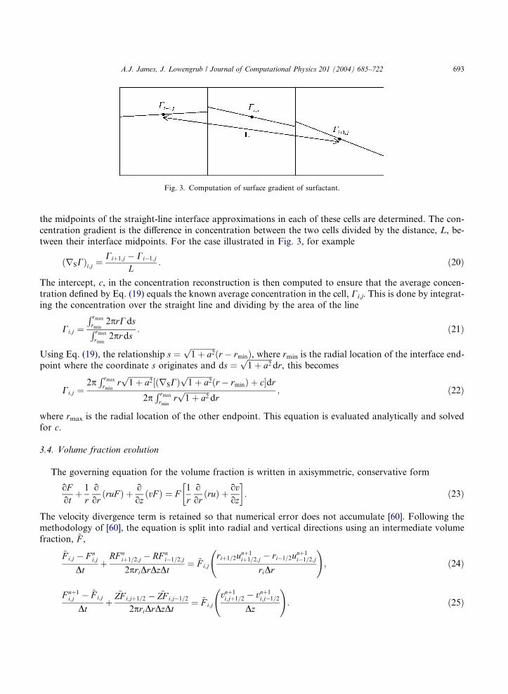
Fig. 3. Computation of surface gradient of surfactant.
A.J. James, J. Lowengrub / Journal of Computational Physics 201 (2004) 685–722 693
the midpoints of the straight-line interface approximations in each of these cells are determined. The con-
centration gradient is the difference in concentration between the two cells divided by the distance, L, be-
tween their interface midpoints. For the case illustrated in Fig. 3, for example
ðrSCÞi;j ¼Ciþ1;j � Ci�1;j
L: ð20Þ
The intercept, c, in the concentration reconstruction is then computed to ensure that the average concen-
tration defined by Eq. (19) equals the known average concentration in the cell, Ci,j. This is done by integrat-ing the concentration over the straight line and dividing by the area of the line
Ci;j ¼R rmax
rmin2prCdsR rmax
rmin2prds
: ð21Þ
Using Eq. (19), the relationship s ¼ffiffiffiffiffiffiffiffiffiffiffiffiffi1þ a2
pðr � rminÞ, where rmin is the radial location of the interface end-
point where the coordinate s originates and ds ¼ffiffiffiffiffiffiffiffiffiffiffiffiffi1þ a2
pdr, this becomes
Ci;j ¼2pR rmax
rminrffiffiffiffiffiffiffiffiffiffiffiffiffi1þ a2
p½ðrSCÞ
ffiffiffiffiffiffiffiffiffiffiffiffiffi1þ a2
pðr � rminÞ þ c�dr
2pR rmax
rminrffiffiffiffiffiffiffiffiffiffiffiffiffi1þ a2
pdr
; ð22Þ
where rmax is the radial location of the other endpoint. This equation is evaluated analytically and solved
for c.
3.4. Volume fraction evolution
The governing equation for the volume fraction is written in axisymmetric, conservative form
oFot
þ 1
ro
orðruF Þ þ o
ozðvF Þ ¼ F
1
ro
orðruÞ þ ov
oz
� �: ð23Þ
The velocity divergence term is retained so that numerical error does not accumulate [60]. Following the
methodology of [60], the equation is split into radial and vertical directions using an intermediate volume
fraction, ~F ,
~F i;j � F ni;j
DtþRF n
iþ1=2;j � RF ni�1=2;j
2priDrDzDt¼ ~F i;j
riþ1=2unþ1iþ1=2;j � ri�1=2unþ1
i�1=2;j
riDr
!; ð24Þ
F nþ1i;j � ~F i;j
Dtþ
~ZF i;jþ1=2 � ~ZF i;j�1=2
2priDrDzDt¼ ~F i;j
vnþ1i;jþ1=2 � vnþ1
i;j�1=2
Dz
!: ð25Þ
694 A.J. James, J. Lowengrub / Journal of Computational Physics 201 (2004) 685–722
RFi+1/2, j is the volume flux of fluid 1 in the radial direction across the ðiþ 12; jÞ face and ZFi, j+1/2 is the
volume flux of fluid 1 in the vertical direction across the ði; jþ 12Þ face. The volume of a grid cell is 2priDrDz.
The fluxes are calculated in one direction and used to update the volume fraction to the intermediate level.
Then, using the intermediate volume fraction, the fluxes are calculated in the other direction and used to
update the intermediate volume fraction to the next time level. The direction computed first is switchedat each time step.
The volume flux is the amount of fluid 1 that passes through the face during the time step. This flux
equals the amount of fluid 1 in the domain of dependence of the face, at the beginning of the time step.
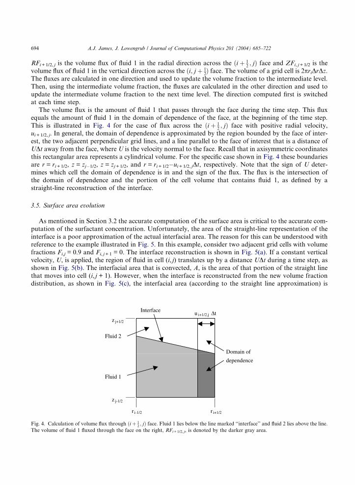
This is illustrated in Fig. 4 for the case of flux across the ðiþ 12; jÞ face with positive radial velocity,
ui+1/2, j. In general, the domain of dependence is approximated by the region bounded by the face of inter-
est, the two adjacent perpendicular grid lines, and a line parallel to the face of interest that is a distance of
UDt away from the face, where U is the velocity normal to the face. Recall that in axisymmetric coordinates
this rectangular area represents a cylindrical volume. For the specific case shown in Fig. 4 these boundariesare r = ri+1/2, z = zj�1/2, z = zj+1/2, and r = ri+1/2�ui+1/2, jDt, respectively. Note that the sign of U deter-
mines which cell the domain of dependence is in and the sign of the flux. The flux is the intersection of
the domain of dependence and the portion of the cell volume that contains fluid 1, as defined by a
straight-line reconstruction of the interface.
3.5. Surface area evolution
As mentioned in Section 3.2 the accurate computation of the surface area is critical to the accurate com-putation of the surfactant concentration. Unfortunately, the area of the straight-line representation of the
interface is a poor approximation of the actual interfacial area. The reason for this can be understood with
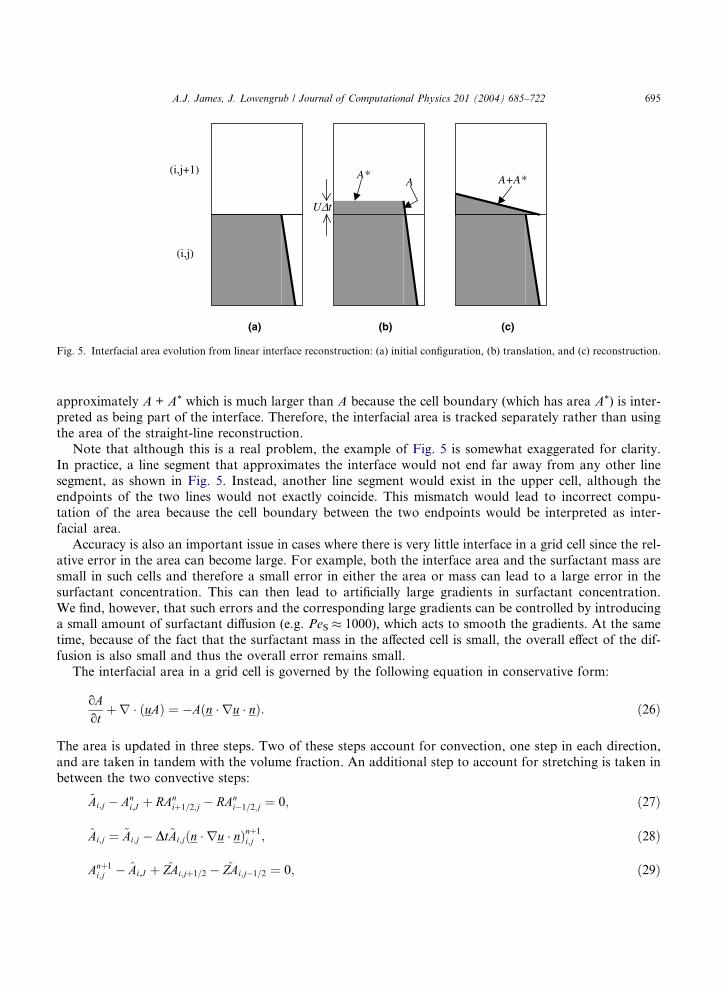
reference to the example illustrated in Fig. 5. In this example, consider two adjacent grid cells with volume
fractions Fi,j = 0.9 and Fi, j+1 = 0. The interface reconstruction is shown in Fig. 5(a). If a constant vertical
velocity, U, is applied, the region of fluid in cell (i, j) translates up by a distance UDt during a time step, as
shown in Fig. 5(b). The interfacial area that is convected, A, is the area of that portion of the straight line
that moves into cell (i, j + 1). However, when the interface is reconstructed from the new volume fraction
distribution, as shown in Fig. 5(c), the interfacial area (according to the straight line approximation) is
Interface u i+1/2,j ∆t
r i-1/2 r i+1/2
z j+1/2
z j-1/2
Fluid 1
Fluid 2
Domain of
dependence
Fig. 4. Calculation of volume flux through ðiþ 12; jÞ face. Fluid 1 lies below the line marked ‘‘interface’’ and fluid 2 lies above the line.
The volume of fluid 1 fluxed through the face on the right, RFi+1/2, j, is denoted by the darker gray area.
(i,j+1)
(i,j)
U∆t
AA* A+A*
(a) (b) (c)
Fig. 5. Interfacial area evolution from linear interface reconstruction: (a) initial configuration, (b) translation, and (c) reconstruction.
A.J. James, J. Lowengrub / Journal of Computational Physics 201 (2004) 685–722 695
approximately A + A* which is much larger than A because the cell boundary (which has area A*) is inter-
preted as being part of the interface. Therefore, the interfacial area is tracked separately rather than using
the area of the straight-line reconstruction.
Note that although this is a real problem, the example of Fig. 5 is somewhat exaggerated for clarity.
In practice, a line segment that approximates the interface would not end far away from any other line
segment, as shown in Fig. 5. Instead, another line segment would exist in the upper cell, although theendpoints of the two lines would not exactly coincide. This mismatch would lead to incorrect compu-
tation of the area because the cell boundary between the two endpoints would be interpreted as inter-
facial area.
Accuracy is also an important issue in cases where there is very little interface in a grid cell since the rel-
ative error in the area can become large. For example, both the interface area and the surfactant mass are
small in such cells and therefore a small error in either the area or mass can lead to a large error in the
surfactant concentration. This can then lead to artificially large gradients in surfactant concentration.
We find, however, that such errors and the corresponding large gradients can be controlled by introducinga small amount of surfactant diffusion (e.g. PeS � 1000), which acts to smooth the gradients. At the same
time, because of the fact that the surfactant mass in the affected cell is small, the overall effect of the dif-
fusion is also small and thus the overall error remains small.
The interfacial area in a grid cell is governed by the following equation in conservative form:
oAot
þr � ðuAÞ ¼ �Aðn � ru � nÞ: ð26Þ
The area is updated in three steps. Two of these steps account for convection, one step in each direction,
and are taken in tandem with the volume fraction. An additional step to account for stretching is taken in
between the two convective steps:
~Ai;j � Ani;J þ RAn
iþ1=2;j � RAni�1=2;j ¼ 0; ð27Þ
Ai;j ¼ ~Ai;j � Dt~Ai;j n � ru � nð Þnþ1
i;j ; ð28Þ
Anþ1i;j � Ai;J þ ZAi;jþ1=2 � ZAi;j�1=2 ¼ 0; ð29Þ
696 A.J. James, J. Lowengrub / Journal of Computational Physics 201 (2004) 685–722
where RAniþ1=2;j is the interfacial area flux in the radial direction across the ðiþ 1
2; jÞ face, and ZAn
i;jþ1=2 is the
interfacial area flux in the vertical direction across the ði; jþ 12Þ face. The stretching term in Eq. (28) is eval-
uated with second-order central differences. Convective fluxes of area are computed analogously to the vol-
ume fraction fluxes, and, as for the volume fraction, the direction computed first is switched at each time
step. The fluxes in one direction are used to update the area to an intermediate value in all cells, ~A, at thesame time the volume fraction is updated by convection in the same direction. The straight line interface
reconstruction is then updated. Next, stretching is applied to update the area in all cells to A. Finally, con-vective fluxes in the other direction complete the update of the area in all cells to the new time step, An + 1.
This is done in conjunction with the final update of the volume fraction by convection in the same direction.
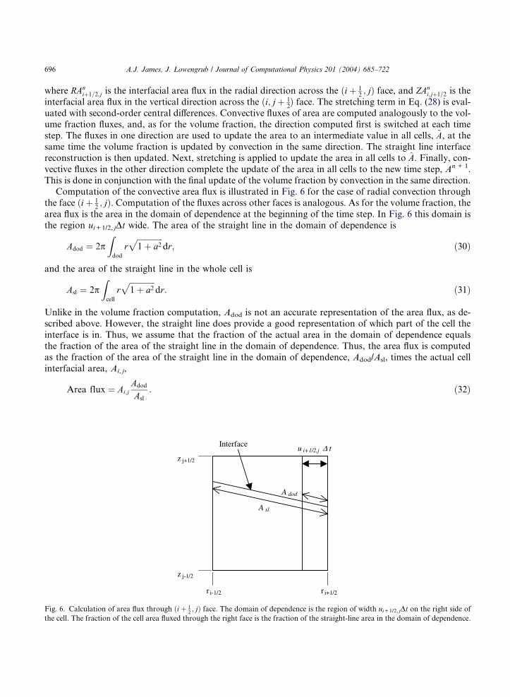
Computation of the convective area flux is illustrated in Fig. 6 for the case of radial convection through
the face ðiþ 12; jÞ. Computation of the fluxes across other faces is analogous. As for the volume fraction, the
area flux is the area in the domain of dependence at the beginning of the time step. In Fig. 6 this domain is
the region ui+1/2, jDt wide. The area of the straight line in the domain of dependence is
Fig. 6.
the cel
Adod ¼ 2pZdod
rffiffiffiffiffiffiffiffiffiffiffiffiffi1þ a2
pdr; ð30Þ
and the area of the straight line in the whole cell is
Asl ¼ 2pZcell
rffiffiffiffiffiffiffiffiffiffiffiffiffi1þ a2
pdr: ð31Þ
Unlike in the volume fraction computation, Adod is not an accurate representation of the area flux, as de-
scribed above. However, the straight line does provide a good representation of which part of the cell the
interface is in. Thus, we assume that the fraction of the actual area in the domain of dependence equals
the fraction of the area of the straight line in the domain of dependence. Thus, the area flux is computed
as the fraction of the area of the straight line in the domain of dependence, Adod/Asl, times the actual cell
interfacial area, Ai, j,
Area flux ¼ Ai;jAdod
Asl
: ð32Þ
Interfaceu i+1/2,j ∆ t
r i-1/2 r i+1/2
z j+1/2
z j-1/2
A dod
A sl
Calculation of area flux through ðiþ 12; jÞ face. The domain of dependence is the region of width ui+1/2, jDt on the right side of
l. The fraction of the cell area fluxed through the right face is the fraction of the straight-line area in the domain of dependence.
A.J. James, J. Lowengrub / Journal of Computational Physics 201 (2004) 685–722 697
Current efforts are focused on developing a higher-order representation of the interface using parabolic seg-
ments. In this method the interface reconstruction will track the interfacial area correctly, making the
reconstruction consistent with both the volume fraction and the area.
3.6. Surfactant evolution
Rather than solving Eq. (5) for the surfactant concentration, the surfactant mass is tracked. This
approach has the advantage that surfactant mass conservation can be enforced directly. The concen-
tration is also determined since it determines the surface tension and its gradient drives surface
diffusion.
The evolution of the surfactant mass in a cell is governed by the following conservative convection–dif-
fusion equation:
oMot
þr � ðuMÞ ¼ APeS
r2SC: ð33Þ
At each time step, the mass equations are updated in three steps that correspond to convection anddiffusion.
~Mi;j �Mni;J þ RMn
iþ1=2;j � RMni�1=2;j ¼ 0; ð34Þ
M i;j � ~Mi;J þ ~ZMi;jþ1=2 � ~ZMi;j�1=2 ¼ 0; ð35Þ
Mnþ1i;j � M i;j ¼ DRnþ1
iþ1=2;j � DRnþ1i�1=2;j þ DZnþ1
i;jþ1=2 � DZnþ1i;j�1=2: ð36Þ
First, the mass is updated in every cell to an intermediate level, ~M , by convection in one direction, along the
convection of volume fraction and interfacial area in the same direction. After this the interface approxi-
mation is reconstructed, the area is stretched, the average concentration is updated as C = M/A, Eq. (6),
and the concentration approximation is reconstructed. Next, the mass is updated in every cell by convection
in the other direction to M , along with convection of volume fraction and interfacial area. The direction inwhich F, A and M are convected first is switched at every time step to avoid skew. Then, once again, the
interface approximation is reconstructed, the average concentration is updated using Eq. (6), and the con-
centration approximation is reconstructed. Finally, the mass is updated in every cell to the next time level,
Mn + 1, by diffusion in both directions simultaneously.
The mass fluxed by convection through a cell face during a time step equals the mass in the domain of
dependence at the beginning of the step, as for volume of fluid and interfacial area. Its computation is anal-
ogous to the area flux computation. A first approximation to the flux is the integral of the concentration
over the straight line in the domain of dependence
Mdod ¼ 2pZdod
rffiffiffiffiffiffiffiffiffiffiffiffiffi1þ a2
p½ðrSCÞ
ffiffiffiffiffiffiffiffiffiffiffiffiffi1þ a2
pðr � rminÞ þ c�dr: ð37Þ
In Eq. (37) it is crucial to use the linear reconstruction of the concentration, instead of simply its average
value, to avoid excessive numerical diffusion. As for the area, this does not accurately represent the flux
since Mdod is obtained using the straight line. However, Mdod/Adod gives a consistent value for the average
concentration on the portion of the interface that is convected. This is multiplied by the area flux to obtaina mass flux that is consistent with the area flux
Mass flux ¼ Mdod
Adod
� �Ai;j
Adod
Asl
� �: ð38Þ
698 A.J. James, J. Lowengrub / Journal of Computational Physics 201 (2004) 685–722
Next, the mass is updated to the new time step by diffusion in a single implicit step. Diffusion of surfactant
across a cell face occurs only when there is an interface in both cells adjacent to the face. From Fick�s law,the radial flux across the face ðiþ 1
2; jÞ, for example, is
DRnþ1iþ1=2;j ¼
DtPeS
2priþ1=2
oCos
� �nþ1
iþ1=2;j
: ð39Þ
This can also be obtained from Eq. (11) as follows. For axisymmetric coordinates n� nV ¼ �h (the azi-
muthal direction) is the tangent to curve C, n� nV � n is the tangent to the interface in the r�z plane point-
ing out of the grid cell, and so ðn� nV � nÞ � rSC becomes the scalar derivative of C in this tangent
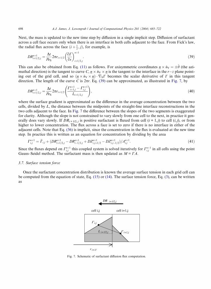
direction. The length of the curve C is 2pr. Eq. (39) can be approximated, as illustrated in Fig. 7, by
DRnþ1iþ1=2;j ¼
DtPeS
2priþ1=2
Cnþ1iþ1;j � Cnþ1
i;j
Liþ1=2;j
!; ð40Þ
where the surface gradient is approximated as the difference in the average concentration between the two
cells, divided by L, the distance between the midpoints of the straight-line interface reconstructions in the
two cells adjacent to the face. In Fig. 7 the difference between the slopes of the two segments is exaggerated
for clarity. Although the slope is not constrained to vary slowly from one cell to the next, in practice it gen-erally does vary slowly. If DRi+1/2, j is positive surfactant is fluxed from cell (i + 1, j) to cell (i, j), or from
higher to lower concentration. The flux across a face is set to zero if there is no interface in either of the
adjacent cells. Note that Eq. (36) is implicit, since the concentration in the flux is evaluated at the new time
step. In practice this is written as an equation for concentration by dividing by the area
Cnþ1i;j ¼ Ci;j þ ðDRnþ1
iþ1=2;j � DRnþ1i�1=2;j þ DZnþ1
i;jþ1=2 � DZnþ1i;j�1=2Þ=Anþ1
i;j : ð41Þ
Since the fluxes depend on Cnþ1i;j this coupled system is solved iteratively for Cnþ1
i;j in all cells using the point
Gauss–Seidel method. The surfactant mass is then updated as M = CA.
3.7. Surface tension force
Once the surfactant concentration distribution is known the average surface tension in each grid cell can
be computed from the equation of state, Eq. (15) or (14). The surface tension force, Eq. (3), can be written
as
cell i,j cell i+1,j
Γ i,j
Γ i+1,jL i+1/2,j
r i+1/
DR i+1/2,j
Fig. 7. Schematic of surfactant diffusion flux computation.
A.J. James, J. Lowengrub / Journal of Computational Physics 201 (2004) 685–722 699
F S ¼ rjrF þ oros
jrF js: ð42Þ
In the staggered grid arrangement the radial component of this force is computed at ðiþ 12; jÞ cell faces and
the vertical component at ði; jþ 12Þ cell faces. First, the curvature is computed in each grid cell center from a
smoothed volume fraction using standard methods [35]. Next, the curvature is evaluated at each face as the
average of the curvature in the two adjacent cells, e.g.
jiþ1=2;j ¼ji;j þ jiþ1;j
2: ð43Þ
The surface tension at cells faces is also computed as the average of the surface tension in the two adjacent
cells, if both cells contain an interface segment. If only one of the adjacent cells contains an interface seg-
ment the surface tension in that cell is used as the surface tension at the face. If there is not an interface
segment in either adjacent cell the surface tension at the face is set to zero and there is no normal force.
The surface gradient of the surface tension is also non-zero only at faces for which both adjacent gridcells contain an interface segment. For such faces the gradient is computed exactly as the surface gradient
of concentration is computed in evaluating surface diffusion, as illustrated in Fig. 7. First the distance be-
tween the interface midpoints is computed. The gradient is then the difference in the surface tension between
the two cells divided by this distance, L. Since the cell face is not necessarily halfway between the interface
midpoints the method is not strictly second order accurate in space. The magnitude of the volume fraction
gradient at each face is computed using straightforward second-order finite difference approximations. Fi-
nally, the radial and vertical components of the surface stress, FR and FZ, respectively, are
FRiþ1=2;j ¼ ðrjÞiþ1=2;j
F iþ1;j � F i;j
Dr
� �þ riþ1;j � ri;j
Liþ1=2;j
� �jrF jiþ1=2;j; ð44Þ
FZi;jþ1=2 ¼ ðrjÞi;jþ1=2
F i;jþ1 � F i;j
Dz
� �þ ri;jþ1 � ri;j
Li;jþ1=2
� �jrF ji;jþ1=2: ð45Þ
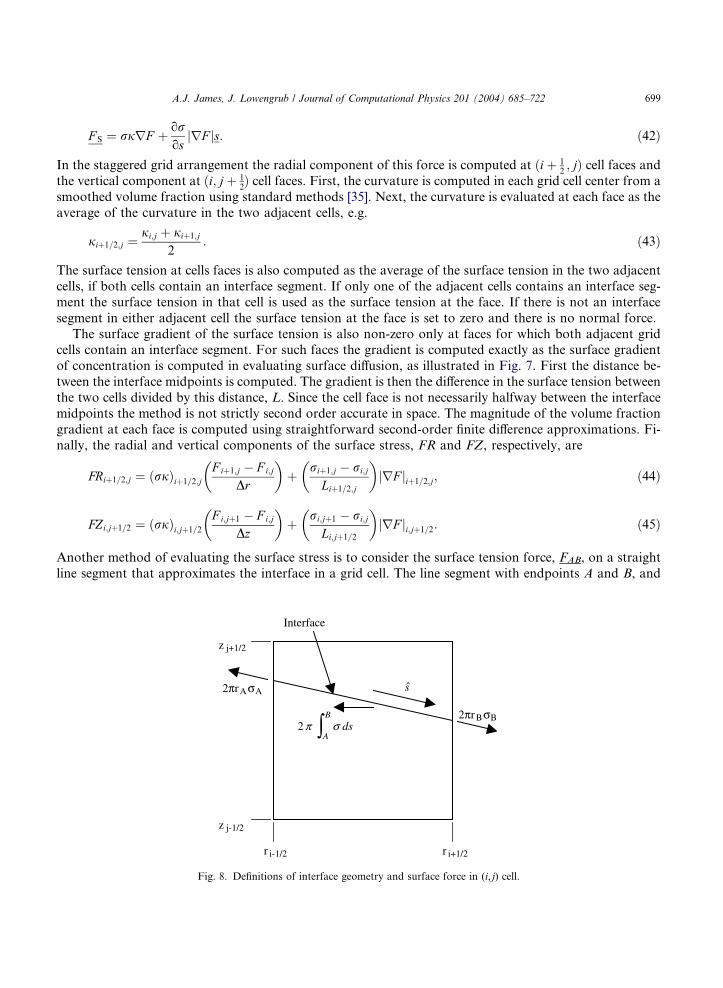
Another method of evaluating the surface stress is to consider the surface tension force, FAB, on a straight
line segment that approximates the interface in a grid cell. The line segment with endpoints A and B, and
∫B
Adsσπ2
Interface
r i-1/2 r i+1/2
z j+1/2
z j-1/2
2πrAσA
2πrBσB
s
Fig. 8. Definitions of interface geometry and surface force in (i, j) cell.
700 A.J. James, J. Lowengrub / Journal of Computational Physics 201 (2004) 685–722
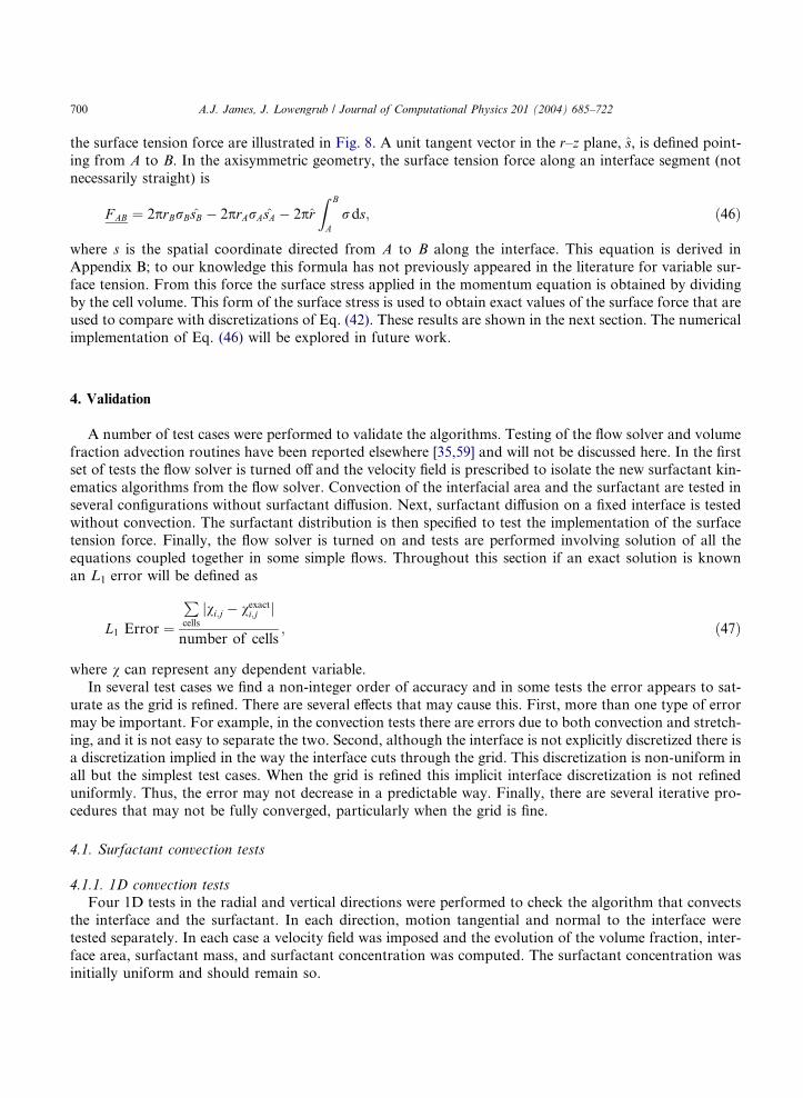
the surface tension force are illustrated in Fig. 8. A unit tangent vector in the r–z plane, s, is defined point-
ing from A to B. In the axisymmetric geometry, the surface tension force along an interface segment (not
necessarily straight) is
F AB ¼ 2prBrBsB � 2prArAsA � 2prZ B
Ards; ð46Þ
where s is the spatial coordinate directed from A to B along the interface. This equation is derived in
Appendix B; to our knowledge this formula has not previously appeared in the literature for variable sur-
face tension. From this force the surface stress applied in the momentum equation is obtained by dividing
by the cell volume. This form of the surface stress is used to obtain exact values of the surface force that areused to compare with discretizations of Eq. (42). These results are shown in the next section. The numerical
implementation of Eq. (46) will be explored in future work.
4. Validation
A number of test cases were performed to validate the algorithms. Testing of the flow solver and volume
fraction advection routines have been reported elsewhere [35,59] and will not be discussed here. In the firstset of tests the flow solver is turned off and the velocity field is prescribed to isolate the new surfactant kin-
ematics algorithms from the flow solver. Convection of the interfacial area and the surfactant are tested in
several configurations without surfactant diffusion. Next, surfactant diffusion on a fixed interface is tested
without convection. The surfactant distribution is then specified to test the implementation of the surface
tension force. Finally, the flow solver is turned on and tests are performed involving solution of all the
equations coupled together in some simple flows. Throughout this section if an exact solution is known
an L1 error will be defined as
L1 Error ¼
Pcells
jvi;j � vexacti;j j
number of cells; ð47Þ
where v can represent any dependent variable.
In several test cases we find a non-integer order of accuracy and in some tests the error appears to sat-
urate as the grid is refined. There are several effects that may cause this. First, more than one type of error
may be important. For example, in the convection tests there are errors due to both convection and stretch-
ing, and it is not easy to separate the two. Second, although the interface is not explicitly discretized there isa discretization implied in the way the interface cuts through the grid. This discretization is non-uniform in
all but the simplest test cases. When the grid is refined this implicit interface discretization is not refined
uniformly. Thus, the error may not decrease in a predictable way. Finally, there are several iterative pro-
cedures that may not be fully converged, particularly when the grid is fine.
4.1. Surfactant convection tests
4.1.1. 1D convection tests
Four 1D tests in the radial and vertical directions were performed to check the algorithm that convects
the interface and the surfactant. In each direction, motion tangential and normal to the interface were
tested separately. In each case a velocity field was imposed and the evolution of the volume fraction, inter-
face area, surfactant mass, and surfactant concentration was computed. The surfactant concentration was
initially uniform and should remain so.
A.J. James, J. Lowengrub / Journal of Computational Physics 201 (2004) 685–722 701
In the first three tests the interface was represented exactly by the staight line reconstruction, so the re-
sults were exact within round-off error. These tests were: (i) radial convection of surfactant along a fixed
horizontal interface, (ii) vertical convection of surfactant along a fixed vertical interface, and (iii) vertical
convection of surfactant with a vertically translating horizontal interface.
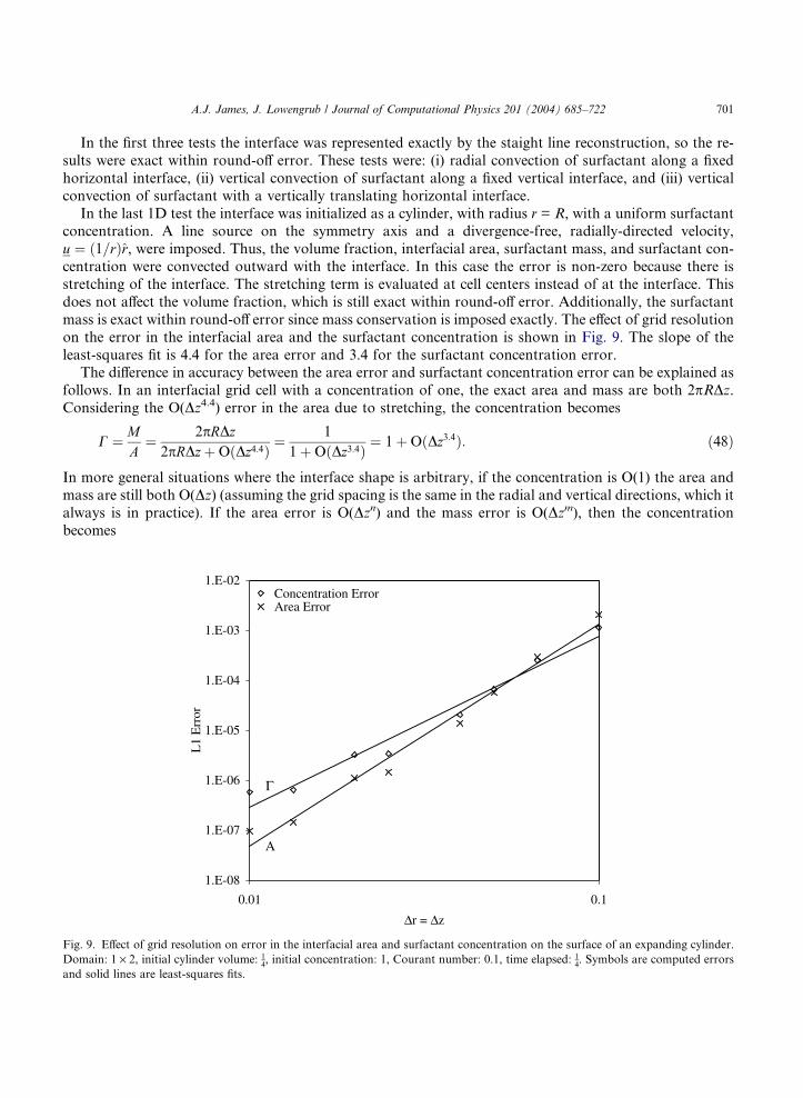
In the last 1D test the interface was initialized as a cylinder, with radius r = R, with a uniform surfactantconcentration. A line source on the symmetry axis and a divergence-free, radially-directed velocity,
u ¼ ð1=rÞr, were imposed. Thus, the volume fraction, interfacial area, surfactant mass, and surfactant con-
centration were convected outward with the interface. In this case the error is non-zero because there is
stretching of the interface. The stretching term is evaluated at cell centers instead of at the interface. This
does not affect the volume fraction, which is still exact within round-off error. Additionally, the surfactant
mass is exact within round-off error since mass conservation is imposed exactly. The effect of grid resolution
on the error in the interfacial area and the surfactant concentration is shown in Fig. 9. The slope of the
least-squares fit is 4.4 for the area error and 3.4 for the surfactant concentration error.The difference in accuracy between the area error and surfactant concentration error can be explained as
follows. In an interfacial grid cell with a concentration of one, the exact area and mass are both 2pRDz.Considering the O(Dz4.4) error in the area due to stretching, the concentration becomes
Fig. 9.
Doma
and so
C ¼ MA
¼ 2pRDz2pRDzþOðDz4:4Þ ¼
1
1þOðDz3:4Þ ¼ 1þOðDz3:4Þ: ð48Þ
In more general situations where the interface shape is arbitrary, if the concentration is O(1) the area and
mass are still both O(Dz) (assuming the grid spacing is the same in the radial and vertical directions, which it
always is in practice). If the area error is O(Dzn) and the mass error is O(Dzm), then the concentration
becomes
1.E-08
1.E-07
1.E-06
1.E-05
1.E-04
1.E-03
1.E-02
0.01 0.1
∆r = ∆z
L1
Err
or
Γ
A
Concentration ErrorArea Error
Effect of grid resolution on error in the interfacial area and surfactant concentration on the surface of an expanding cylinder.
in: 1 · 2, initial cylinder volume: 14, initial concentration: 1, Courant number: 0.1, time elapsed: 1
4. Symbols are computed errors
lid lines are least-squares fits.
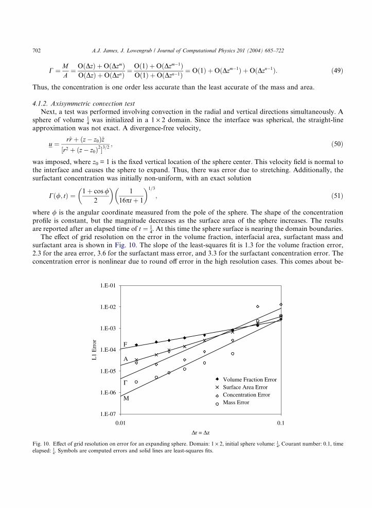
Fig. 10
elapse
702 A.J. James, J. Lowengrub / Journal of Computational Physics 201 (2004) 685–722
C ¼ MA
¼ OðDzÞ þOðDzmÞOðDzÞ þOðDznÞ ¼
Oð1Þ þOðDzm�1ÞOð1Þ þOðDzn�1Þ ¼ Oð1Þ þOðDzm�1Þ þOðDzn�1Þ: ð49Þ
Thus, the concentration is one order less accurate than the least accurate of the mass and area.
4.1.2. Axisymmetric convection test
Next, a test was performed involving convection in the radial and vertical directions simultaneously. A
sphere of volume 14was initialized in a 1 · 2 domain. Since the interface was spherical, the straight-line
approximation was not exact. A divergence-free velocity,
u ¼ rr þ ðz� z0Þz½r2 þ ðz� z0Þ2�3=2
; ð50Þ
was imposed, where z0 = 1 is the fixed vertical location of the sphere center. This velocity field is normal tothe interface and causes the sphere to expand. Thus, there was error due to stretching. Additionally, the
surfactant concentration was initially non-uniform, with an exact solution
Cð/; tÞ ¼ 1þ cos/2
� �1
16pt þ 1
� �1=3
; ð51Þ
where / is the angular coordinate measured from the pole of the sphere. The shape of the concentration
profile is constant, but the magnitude decreases as the surface area of the sphere increases. The resultsare reported after an elapsed time of t ¼ 1
4. At this time the sphere surface is nearing the domain boundaries.
The effect of grid resolution on the error in the volume fraction, interfacial area, surfactant mass and
surfactant area is shown in Fig. 10. The slope of the least-squares fit is 1.3 for the volume fraction error,
2.3 for the area error, 3.6 for the surfactant mass error, and 3.3 for the surfactant concentration error. The
concentration error is nonlinear due to round off error in the high resolution cases. This comes about be-
1.E-07
1.E-06
1.E-05
1.E-04
1.E-03
1.E-02
1.E-01
0.01 0.1
∆r = ∆z
L1
Err
or F
M
Γ
A
Volume Fraction ErrorSurface Area ErrorConcentration ErrorMass Error
. Effect of grid resolution on error for an expanding sphere. Domain: 1 · 2, initial sphere volume: 14, Courant number: 0.1, time
d: 14. Symbols are computed errors and solid lines are least-squares fits.
A.J. James, J. Lowengrub / Journal of Computational Physics 201 (2004) 685–722 703
cause the concentration is mass divided by area, which both become small as the grid is refined. Division of
one small number into another is sensitive to round-off errors. Inclusion of a small amount of diffusion in
the computations aleviates this sensitivity by smoothing away the error. The effect of diffusion is illustrated
in the next section.
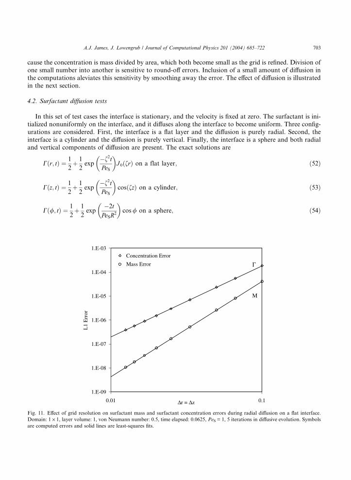
4.2. Surfactant diffusion tests
In this set of test cases the interface is stationary, and the velocity is fixed at zero. The surfactant is ini-
tialized nonuniformly on the interface, and it diffuses along the interface to become uniform. Three config-
urations are considered. First, the interface is a flat layer and the diffusion is purely radial. Second, the
interface is a cylinder and the diffusion is purely vertical. Finally, the interface is a sphere and both radial
and vertical components of diffusion are present. The exact solutions are
Fig. 11
Doma
are com
Cðr; tÞ ¼ 1
2þ 1
2exp
�f2tPeS
� �J 0ðfrÞ on a flat layer; ð52Þ
Cðz; tÞ ¼ 1
2þ 1
2exp
�f2tPeS
� �cosðfzÞ on a cylinder; ð53Þ
Cð/; tÞ ¼ 1
2þ 1
2exp
�2t
PeSR2
� �cos/ on a sphere; ð54Þ
1.E-09
1.E-08
1.E-07
1.E-06
1.E-05
1.E-04
1.E-03
0.01 0.1∆r = ∆z
L1
Err
or
Concentration Error
Mass Error
M
Γ
. Effect of grid resolution on surfactant mass and surfactant concentration errors during radial diffusion on a flat interface.
in: 1 · 1, layer volume: 1, von Neumann number: 0.5, time elapsed: 0.0625, PeS = 1, 5 iterations in diffusive evolution. Symbols
puted errors and solid lines are least-squares fits.
704 A.J. James, J. Lowengrub / Journal of Computational Physics 201 (2004) 685–722
where f is an eigenvalue determined by the boundary conditions, and R is the sphere radius. In each geom-
etry the surfactant mass and concentration are initialized with the exact solution and then allowed to
evolve.
For diffusion on a flat layer of unit volume the domain was 1 · 1 units. The surfactant mass and surf-
actant concentration errors are shown in Fig. 11 as functions of grid resolution. The slope of the least-squares fit is 4.0 for the mass error and 3.0 for the concentration error.
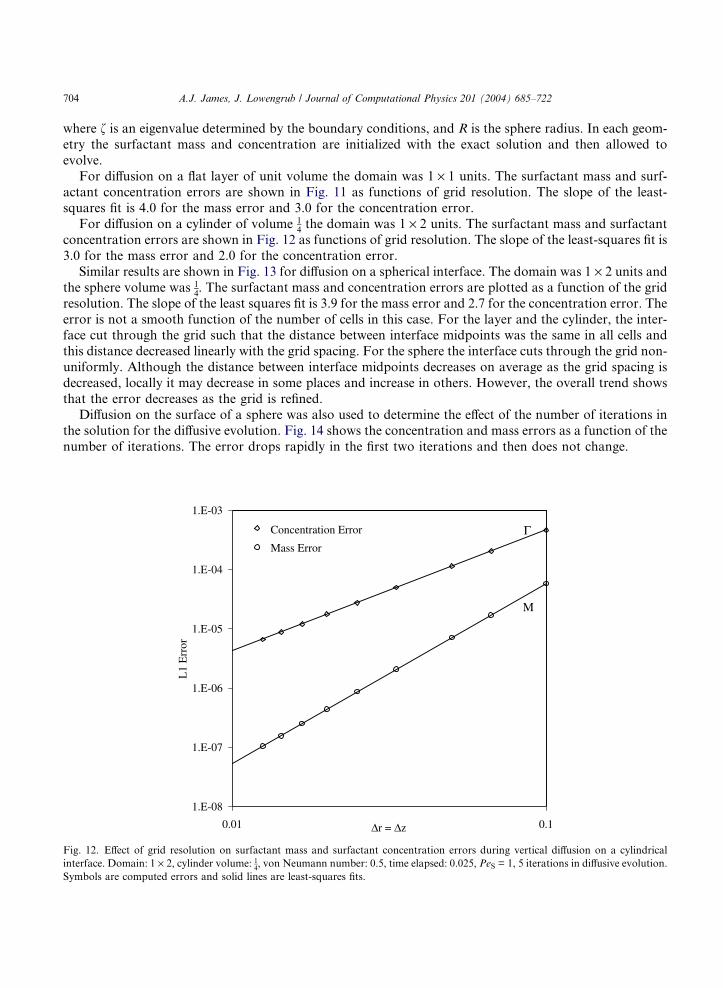
For diffusion on a cylinder of volume 14the domain was 1 · 2 units. The surfactant mass and surfactant
concentration errors are shown in Fig. 12 as functions of grid resolution. The slope of the least-squares fit is
3.0 for the mass error and 2.0 for the concentration error.
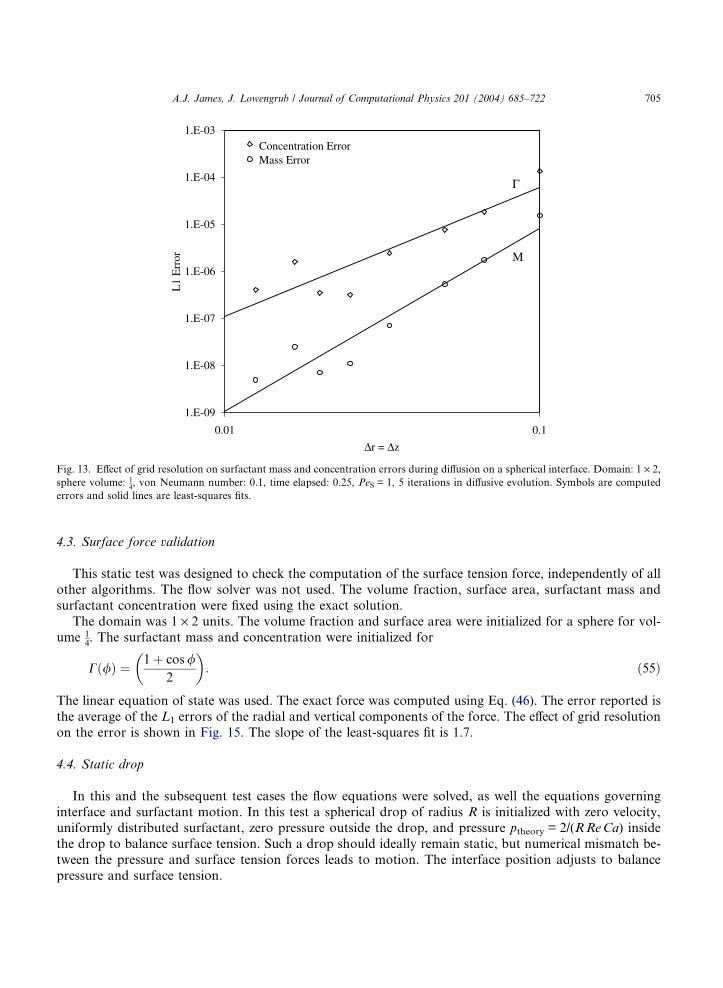
Similar results are shown in Fig. 13 for diffusion on a spherical interface. The domain was 1 · 2 units and
the sphere volume was 14. The surfactant mass and concentration errors are plotted as a function of the grid
resolution. The slope of the least squares fit is 3.9 for the mass error and 2.7 for the concentration error. The
error is not a smooth function of the number of cells in this case. For the layer and the cylinder, the inter-face cut through the grid such that the distance between interface midpoints was the same in all cells and
this distance decreased linearly with the grid spacing. For the sphere the interface cuts through the grid non-
uniformly. Although the distance between interface midpoints decreases on average as the grid spacing is
decreased, locally it may decrease in some places and increase in others. However, the overall trend shows
that the error decreases as the grid is refined.
Diffusion on the surface of a sphere was also used to determine the effect of the number of iterations in
the solution for the diffusive evolution. Fig. 14 shows the concentration and mass errors as a function of the
number of iterations. The error drops rapidly in the first two iterations and then does not change.
1.E-08
1.E-07
1.E-06
1.E-05
1.E-04
1.E-03
0.01 0.1∆r = ∆z
L1
Err
or
M
ΓConcentration Error
Mass Error
Fig. 12. Effect of grid resolution on surfactant mass and surfactant concentration errors during vertical diffusion on a cylindrical
interface. Domain: 1 · 2, cylinder volume: 14, von Neumann number: 0.5, time elapsed: 0.025, PeS = 1, 5 iterations in diffusive evolution.
Symbols are computed errors and solid lines are least-squares fits.
1.E-09
1.E-08
1.E-07
1.E-06
1.E-05
1.E-04
1.E-03
0.01 0.1
∆r = ∆z
L1
Err
orΓ
M
Concentration ErrorMass Error
Fig. 13. Effect of grid resolution on surfactant mass and concentration errors during diffusion on a spherical interface. Domain: 1 · 2,
sphere volume: 14, von Neumann number: 0.1, time elapsed: 0.25, PeS = 1, 5 iterations in diffusive evolution. Symbols are computed
errors and solid lines are least-squares fits.
A.J. James, J. Lowengrub / Journal of Computational Physics 201 (2004) 685–722 705
4.3. Surface force validation
This static test was designed to check the computation of the surface tension force, independently of all
other algorithms. The flow solver was not used. The volume fraction, surface area, surfactant mass and
surfactant concentration were fixed using the exact solution.
The domain was 1 · 2 units. The volume fraction and surface area were initialized for a sphere for vol-
ume 14. The surfactant mass and concentration were initialized for
Cð/Þ ¼ 1þ cos/2
� �: ð55Þ
The linear equation of state was used. The exact force was computed using Eq. (46). The error reported is
the average of the L1 errors of the radial and vertical components of the force. The effect of grid resolution
on the error is shown in Fig. 15. The slope of the least-squares fit is 1.7.
4.4. Static drop
In this and the subsequent test cases the flow equations were solved, as well the equations governing
interface and surfactant motion. In this test a spherical drop of radius R is initialized with zero velocity,uniformly distributed surfactant, zero pressure outside the drop, and pressure ptheory = 2/(RReCa) inside
the drop to balance surface tension. Such a drop should ideally remain static, but numerical mismatch be-
tween the pressure and surface tension forces leads to motion. The interface position adjusts to balance
pressure and surface tension.

1.E-08
1.E-07
1.E-06
1.E-05
1.E-04
1.E-03
1.E-02
0 1 3 52 4
Number of Iterations
L1
Err
or
Concentration Error
Mass Error
Fig. 14. Effect of the number of iterations in the diffusive evolution on surfactant mass and concentration errors during diffusion on a
spherical interface. Domain: 1 · 2, sphere volume: 14, von Neumann number: 0.1, time elapsed: 0.25, PeS = 1, 30 · 60.
1.E-07
1.E-06
1.E-05
1.E-04
1.E-03
1.E-02
0.001 0.01 0.1
∆r = ∆z
L1
Err
or
Fig. 15. Effect of grid resolution on error in surface tension force. Domain: 1 · 2, sphere volume: 14, b = 0.2. Symbols are computed
error and solid line is least-squares fit.
706 A.J. James, J. Lowengrub / Journal of Computational Physics 201 (2004) 685–722
A.J. James, J. Lowengrub / Journal of Computational Physics 201 (2004) 685–722 707
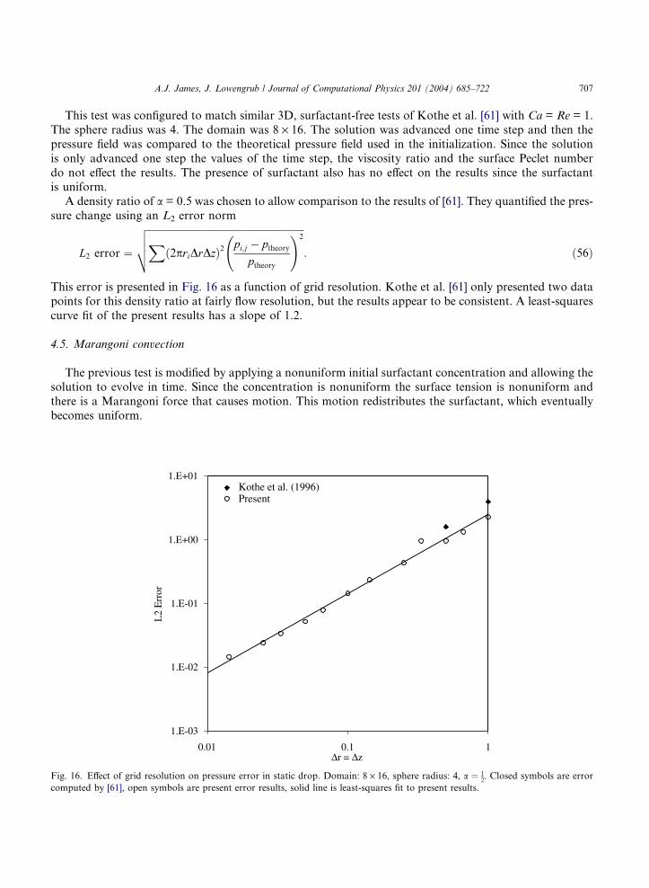
This test was configured to match similar 3D, surfactant-free tests of Kothe et al. [61] with Ca = Re = 1.
The sphere radius was 4. The domain was 8 · 16. The solution was advanced one time step and then the
pressure field was compared to the theoretical pressure field used in the initialization. Since the solution
is only advanced one step the values of the time step, the viscosity ratio and the surface Peclet number
do not effect the results. The presence of surfactant also has no effect on the results since the surfactantis uniform.
A density ratio of a = 0.5 was chosen to allow comparison to the results of [61]. They quantified the pres-
sure change using an L2 error norm
Fig. 16
compu
L2 error ¼
ffiffiffiffiffiffiffiffiffiffiffiffiffiffiffiffiffiffiffiffiffiffiffiffiffiffiffiffiffiffiffiffiffiffiffiffiffiffiffiffiffiffiffiffiffiffiffiffiffiffiffiffiffiffiffiffiffiffiffiffiffiffiffiXð2priDrDzÞ2
pi;j � ptheoryptheory
!2vuut : ð56Þ
This error is presented in Fig. 16 as a function of grid resolution. Kothe et al. [61] only presented two data
points for this density ratio at fairly flow resolution, but the results appear to be consistent. A least-squares
curve fit of the present results has a slope of 1.2.
4.5. Marangoni convection
The previous test is modified by applying a nonuniform initial surfactant concentration and allowing thesolution to evolve in time. Since the concentration is nonuniform the surface tension is nonuniform and
there is a Marangoni force that causes motion. This motion redistributes the surfactant, which eventually
becomes uniform.
1.E-03
1.E-02
1.E-01
1.E+00
1.E+01
0.01 0.1 1∆r = ∆z
L2
Err
or
Kothe et al. (1996)Present
. Effect of grid resolution on pressure error in static drop. Domain: 8 · 16, sphere radius: 4, a ¼ 12. Closed symbols are error
ted by [61], open symbols are present error results, solid line is least-squares fit to present results.
708 A.J. James, J. Lowengrub / Journal of Computational Physics 201 (2004) 685–722
A static sphere with volume 14is initialized in a 1 · 2 domain. The pressure is initally zero outside the
drop and 2/(RReCa) inside the drop to balance the average surface tension force, where R is the sphere
radius. The surfactant mass and concentration are initialized by Eq. (55). The density and viscosity of
the inner and outer fluids are matched and Re = Ca = 1. Both the linear and nonlinear equation of state
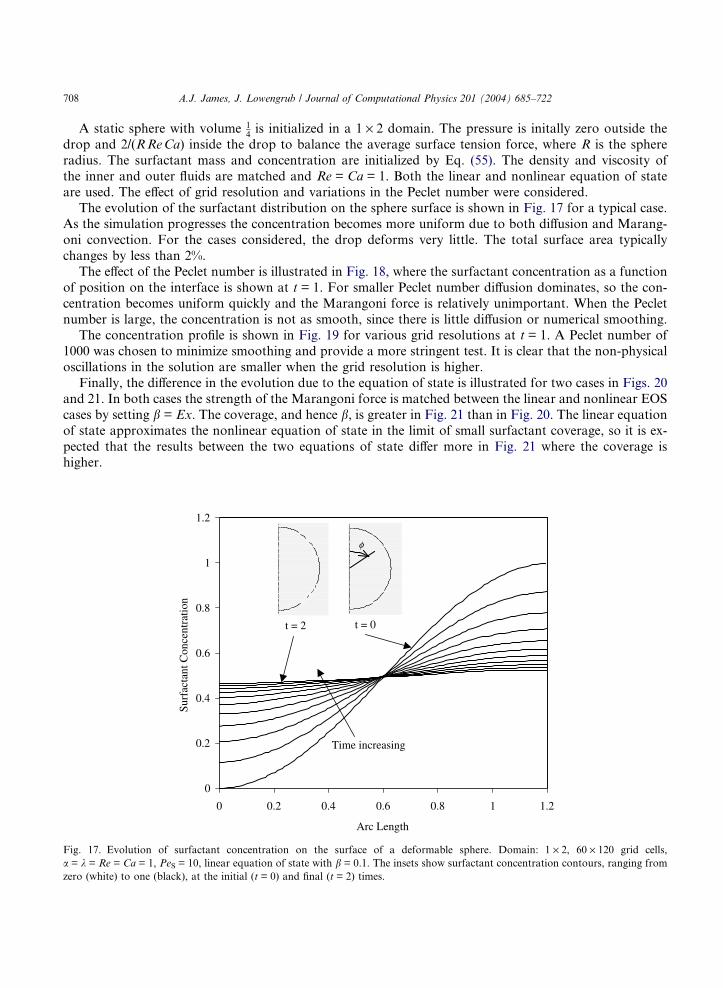
are used. The effect of grid resolution and variations in the Peclet number were considered.The evolution of the surfactant distribution on the sphere surface is shown in Fig. 17 for a typical case.
As the simulation progresses the concentration becomes more uniform due to both diffusion and Marang-
oni convection. For the cases considered, the drop deforms very little. The total surface area typically
changes by less than 2%.
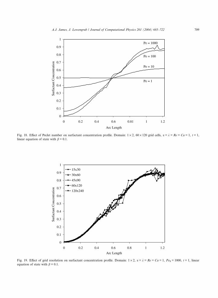
The effect of the Peclet number is illustrated in Fig. 18, where the surfactant concentration as a function
of position on the interface is shown at t = 1. For smaller Peclet number diffusion dominates, so the con-
centration becomes uniform quickly and the Marangoni force is relatively unimportant. When the Peclet
number is large, the concentration is not as smooth, since there is little diffusion or numerical smoothing.The concentration profile is shown in Fig. 19 for various grid resolutions at t = 1. A Peclet number of
1000 was chosen to minimize smoothing and provide a more stringent test. It is clear that the non-physical
oscillations in the solution are smaller when the grid resolution is higher.
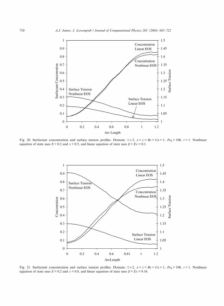
Finally, the difference in the evolution due to the equation of state is illustrated for two cases in Figs. 20
and 21. In both cases the strength of the Marangoni force is matched between the linear and nonlinear EOS
cases by setting b = Ex. The coverage, and hence b, is greater in Fig. 21 than in Fig. 20. The linear equation
of state approximates the nonlinear equation of state in the limit of small surfactant coverage, so it is ex-
pected that the results between the two equations of state differ more in Fig. 21 where the coverage ishigher.
0
0.2
0.4
0.6
0.8
1
1.2
0 0.2 0.4 0.6 0.8 1 1.2
Arc Length
Surf
acta
nt C
once
ntra
tion
Time increasing
φ
t = 0t = 2
φ
Fig. 17. Evolution of surfactant concentration on the surface of a deformable sphere. Domain: 1 · 2, 60 · 120 grid cells,
a = k = Re = Ca = 1, PeS = 10, linear equation of state with b = 0.1. The insets show surfactant concentration contours, ranging from
zero (white) to one (black), at the initial (t = 0) and final (t = 2) times.
0
0.1
0.2
0.3
0.4
0.5
0.6
0.7
0.8
0.9
1
0 0.2 0.4 0.6 0.81 1 1.2
Arc Length
Surf
acta
nt C
once
ntra
tion
Pe = 1
Pe = 10
Pe = 100
Pe = 1000
Fig. 18. Effect of Peclet number on surfactant concentration profile. Domain: 1 · 2, 60 · 120 grid cells, a = k = Re = Ca = 1, t = 1,
linear equation of state with b = 0.1.
0
0.1
0.2
0.3
0.4
0.5
0.6
0.7
0.8
0.9
1
0 0.2 0.4 0.6 0.8 1 1.2
Arc Length
Surf
acta
nt C
once
ntra
tion
15x30
30x60
45x90
60x120
120x240
Fig. 19. Effect of grid resolution on surfactant concentration profile. Domain: 1 · 2, a = k = Re = Ca = 1, PeS = 1000, t = 1, linear
equation of state with b = 0.1.
A.J. James, J. Lowengrub / Journal of Computational Physics 201 (2004) 685–722 709
0
0.1
0.2
0.3
0.4
0.5
0.6
0.7
0.8
0.9
1
0 0.2 0.4 0.6 0.8 1 1.2
Arc Length
Surf
acta
nt C
once
ntra
tion
1
1.05
1.1
1.15
1.2
1.25
1.3
1.35
1.4
1.45
1.5
Surf
ace
Ten
sion
Surface TensionNonlinear EOS
Surface TensionLinear EOS
ConcentrationLinear EOS
ConcentrationNonlinear EOS
Fig. 20. Surfactant concentration and surface tension profiles. Domain: 1 · 2, a = k = Re = Ca = 1, PeS = 100, t = 1. Nonlinear
equation of state uses E = 0.2 and x = 0.5, and linear equation of state uses b = Ex = 0.1.
0
0.1
0.2
0.3
0.4
0.5
0.6
0.7
0.8
0.9
1
0 0.2 0.4 0.6 0.81 1 1.2
ArcLength
Con
cent
ratio
n
1
1.05
1.1
1.15
1.2
1.25
1.3
1.35
1.4
1.45
1.5Su
rfac
e T
ensi
onConcentrationLinear EOS
ConcentrationNonlinear EOS
Surface TensionNonlinear EOS
Surface TensionLinear EOS
Fig. 21. Surfactant concentration and surface tension profiles. Domain: 1 · 2, a = k = Re = Ca = 1, PeS = 100, t = 1. Nonlinear
equation of state uses E = 0.2 and x = 0.8, and linear equation of state uses b = Ex = 0.16.
710 A.J. James, J. Lowengrub / Journal of Computational Physics 201 (2004) 685–722
A.J. James, J. Lowengrub / Journal of Computational Physics 201 (2004) 685–722 711
4.6. Drop extension
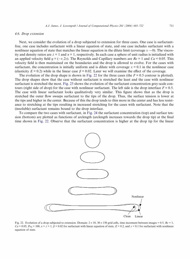
Next, we consider the evolution of a drop subjected to extension for three cases. One case is surfactant-
free, one case includes surfactant with a linear equation of state, and one case includes surfactant with a
nonlinear equation of state that matches the linear equation in the dilute limit (coverage x!0). The viscos-ity and density ratios are k = 1 and a = 1, respectively. In each case a sphere of unit radius is initialized with
an applied velocity field u = (�r, 2z). The Reynolds and Capillary numbers are Re = 1 and Ca = 0.05. This
velocity field is then maintained on the boundaries and the drop is allowed to evolve. For the cases with
surfactant, the concentration is initially uniform and is dilute with coverage x = 0.1 in the nonlinear case
(elasticity E = 0.2) while in the linear case b = 0.02. Later we will examine the effect of the coverage.
The evolution of the drop shape is shown in Fig. 22 for the three cases (the F = 0.5 contour is plotted).
The drop shapes show that the case without surfactant is stretched the least and the case with nonlinear
surfactant is stretched the most. Fig. 23 shows the evolution of the surfactant concentration grey-scale con-tours (right side of drop) for the case with nonlinear surfactant. The left side is the drop interface F = 0.5.
The case with linear surfactant looks qualitatively very similar. This figure shows that as the drop is
stretched the outer flow sweeps surfactant to the tips of the drop. Thus, the surface tension is lower at
the tips and higher in the center. Because of this the drop tends to thin more in the center and has less resist-
ance to stretching at the tips resulting in increased stretching for the cases with surfactant. Note that the
(insoluble) surfactant remains bound to the drop interface.
To compare the two cases with surfactant, in Fig. 24 the surfactant concentration (top) and surface ten-
sion (bottom) are plotted as functions of arclength (arclength increases towards the drop tip) at the finaltime shown in Fig. 22. Observe that the surfactant concentration is higher at the drop tip for the linear
Nonlinear
LinearClean
Fig. 22. Evolution of a drop subjected to extension. Domain: 2 · 10, 30 · 150 grid cells, time increment between images = 0.5, Re = 1,
Ca = 0.05, PeS = 100, a = k = 1, b = 0.02 for surfactant with linear equation of state, E = 0.2, and x = 0.1 for surfactant with nonlinear
equation of state.
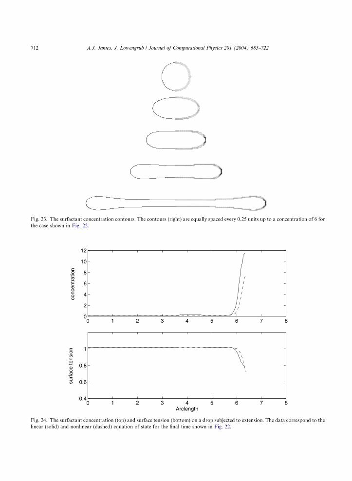
Fig. 23. The surfactant concentration contours. The contours (right) are equally spaced every 0.25 units up to a concentration of 6 for
the case shown in Fig. 22.
0 1 2 3 4 5 6 7 80
2
4
6
8
10
12
conc
entr
atio
n
0 1 2 3 4 5 6 7 80.4
0.6
0.8
1
Arclength
surf
ace
tens
ion
Fig. 24. The surfactant concentration (top) and surface tension (bottom) on a drop subjected to extension. The data correspond to the
linear (solid) and nonlinear (dashed) equation of state for the final time shown in Fig. 22.
712 A.J. James, J. Lowengrub / Journal of Computational Physics 201 (2004) 685–722
0 0.2 0.4 0.6 0.8 1 1.2 1.4 1.6 1.8 20
5
10
15C
once
ntra
tion
0 0.2 0.4 0.6 0.8 1 1.2 1.4 1.6 1.8 20
0.2
0.4
0.6
0.8
1
Time
Sur
face
Ten
sion
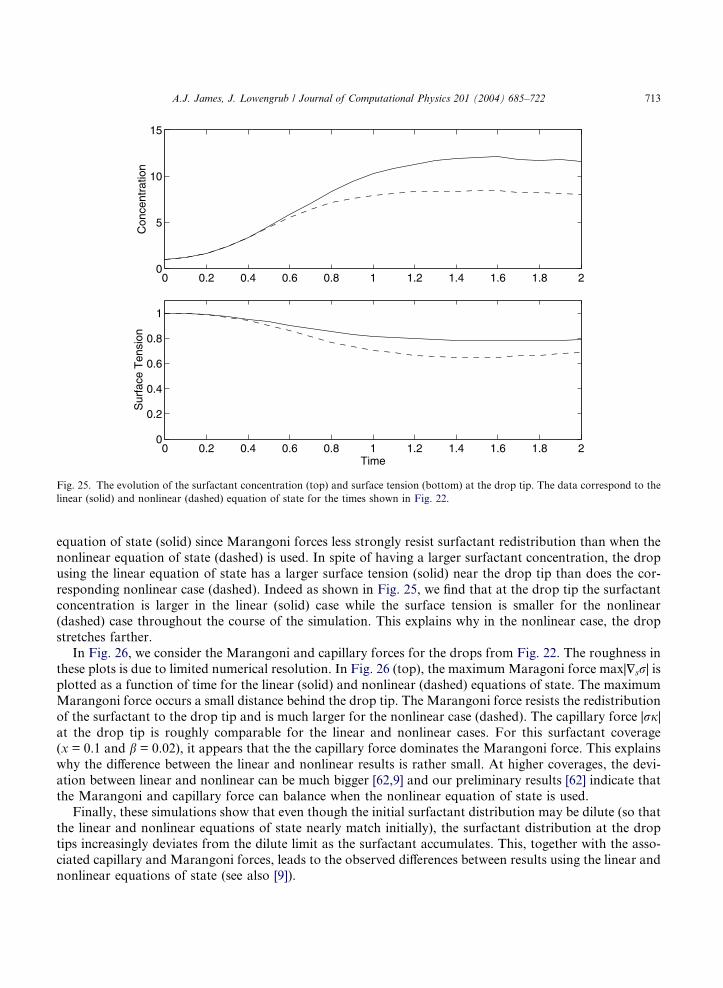
Fig. 25. The evolution of the surfactant concentration (top) and surface tension (bottom) at the drop tip. The data correspond to the
linear (solid) and nonlinear (dashed) equation of state for the times shown in Fig. 22.
A.J. James, J. Lowengrub / Journal of Computational Physics 201 (2004) 685–722 713
equation of state (solid) since Marangoni forces less strongly resist surfactant redistribution than when the
nonlinear equation of state (dashed) is used. In spite of having a larger surfactant concentration, the drop
using the linear equation of state has a larger surface tension (solid) near the drop tip than does the cor-
responding nonlinear case (dashed). Indeed as shown in Fig. 25, we find that at the drop tip the surfactant
concentration is larger in the linear (solid) case while the surface tension is smaller for the nonlinear(dashed) case throughout the course of the simulation. This explains why in the nonlinear case, the drop
stretches farther.
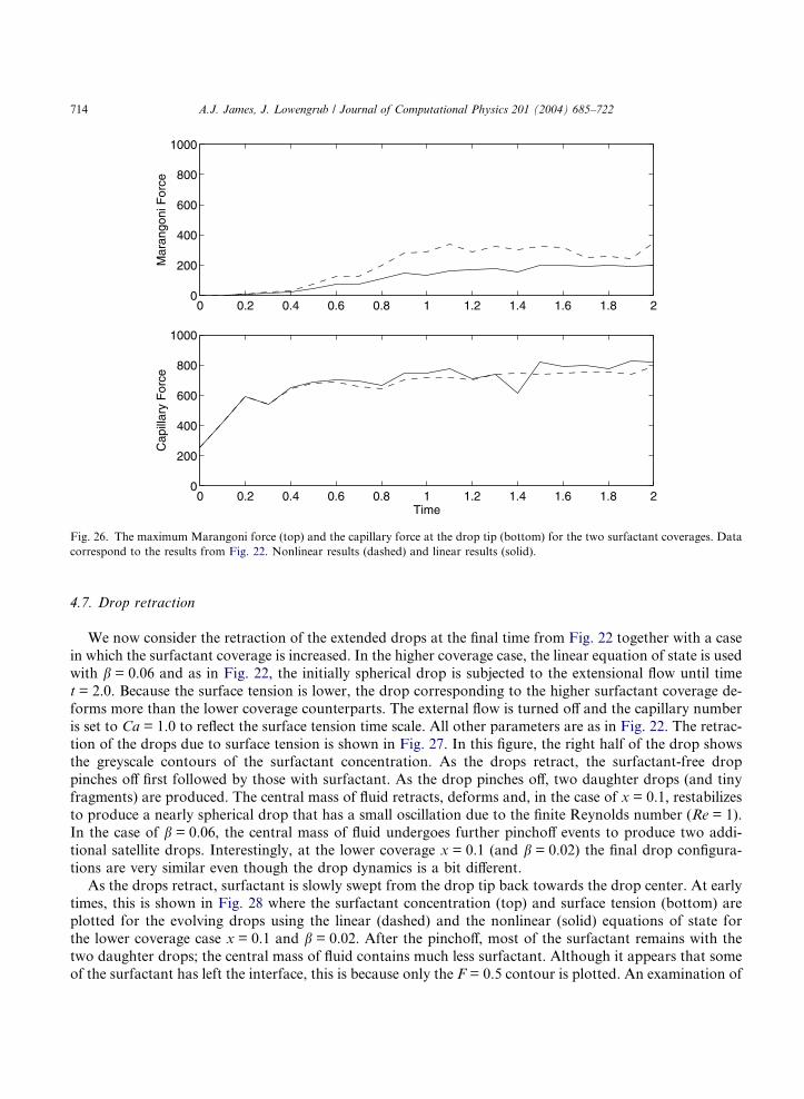
In Fig. 26, we consider the Marangoni and capillary forces for the drops from Fig. 22. The roughness in
these plots is due to limited numerical resolution. In Fig. 26 (top), the maximumMaragoni force max|$sr| isplotted as a function of time for the linear (solid) and nonlinear (dashed) equations of state. The maximum
Marangoni force occurs a small distance behind the drop tip. The Marangoni force resists the redistribution
of the surfactant to the drop tip and is much larger for the nonlinear case (dashed). The capillary force |rj|at the drop tip is roughly comparable for the linear and nonlinear cases. For this surfactant coverage(x = 0.1 and b = 0.02), it appears that the the capillary force dominates the Marangoni force. This explains
why the difference between the linear and nonlinear results is rather small. At higher coverages, the devi-
ation between linear and nonlinear can be much bigger [62,9] and our preliminary results [62] indicate that
the Marangoni and capillary force can balance when the nonlinear equation of state is used.
Finally, these simulations show that even though the initial surfactant distribution may be dilute (so that
the linear and nonlinear equations of state nearly match initially), the surfactant distribution at the drop
tips increasingly deviates from the dilute limit as the surfactant accumulates. This, together with the asso-
ciated capillary and Marangoni forces, leads to the observed differences between results using the linear andnonlinear equations of state (see also [9]).
0 0.2 0.4 0.6 0.8 1 1.2 1.4 1.6 1.8 20
200
400
600
800
1000M
aran
goni
For
ce
0 0.2 0.4 0.6 0.8 1 1.2 1.4 1.6 1.8 20
200
400
600
800
1000
Time
Cap
illar
y F
orce
Fig. 26. The maximum Marangoni force (top) and the capillary force at the drop tip (bottom) for the two surfactant coverages. Data
correspond to the results from Fig. 22. Nonlinear results (dashed) and linear results (solid).
714 A.J. James, J. Lowengrub / Journal of Computational Physics 201 (2004) 685–722
4.7. Drop retraction
We now consider the retraction of the extended drops at the final time from Fig. 22 together with a case
in which the surfactant coverage is increased. In the higher coverage case, the linear equation of state is used
with b = 0.06 and as in Fig. 22, the initially spherical drop is subjected to the extensional flow until time
t = 2.0. Because the surface tension is lower, the drop corresponding to the higher surfactant coverage de-
forms more than the lower coverage counterparts. The external flow is turned off and the capillary number
is set to Ca = 1.0 to reflect the surface tension time scale. All other parameters are as in Fig. 22. The retrac-
tion of the drops due to surface tension is shown in Fig. 27. In this figure, the right half of the drop showsthe greyscale contours of the surfactant concentration. As the drops retract, the surfactant-free drop
pinches off first followed by those with surfactant. As the drop pinches off, two daughter drops (and tiny
fragments) are produced. The central mass of fluid retracts, deforms and, in the case of x = 0.1, restabilizes
to produce a nearly spherical drop that has a small oscillation due to the finite Reynolds number (Re = 1).
In the case of b = 0.06, the central mass of fluid undergoes further pinchoff events to produce two addi-
tional satellite drops. Interestingly, at the lower coverage x = 0.1 (and b = 0.02) the final drop configura-
tions are very similar even though the drop dynamics is a bit different.
As the drops retract, surfactant is slowly swept from the drop tip back towards the drop center. At earlytimes, this is shown in Fig. 28 where the surfactant concentration (top) and surface tension (bottom) are
plotted for the evolving drops using the linear (dashed) and the nonlinear (solid) equations of state for
the lower coverage case x = 0.1 and b = 0.02. After the pinchoff, most of the surfactant remains with the
two daughter drops; the central mass of fluid contains much less surfactant. Although it appears that some
of the surfactant has left the interface, this is because only the F = 0.5 contour is plotted. An examination of
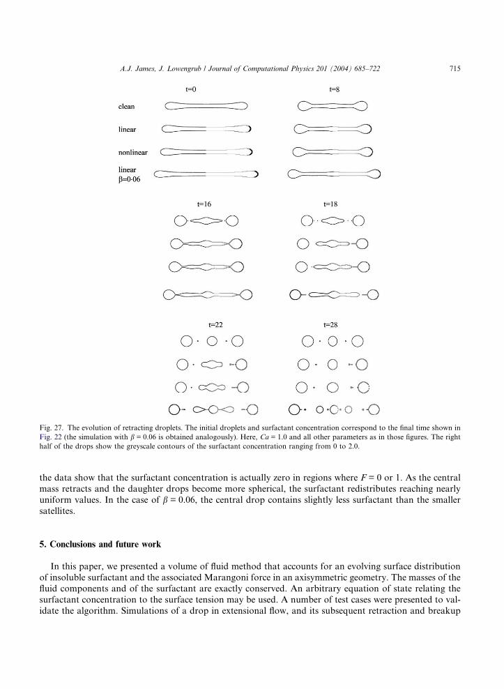
Fig. 27. The evolution of retracting droplets. The initial droplets and surfactant concentration correspond to the final time shown in
Fig. 22 (the simulation with b = 0.06 is obtained analogously). Here, Ca = 1.0 and all other parameters as in those figures. The right
half of the drops show the greyscale contours of the surfactant concentration ranging from 0 to 2.0.
A.J. James, J. Lowengrub / Journal of Computational Physics 201 (2004) 685–722 715
the data show that the surfactant concentration is actually zero in regions where F = 0 or 1. As the central
mass retracts and the daughter drops become more spherical, the surfactant redistributes reaching nearly
uniform values. In the case of b = 0.06, the central drop contains slightly less surfactant than the smaller
satellites.
5. Conclusions and future work
In this paper, we presented a volume of fluid method that accounts for an evolving surface distribution
of insoluble surfactant and the associated Marangoni force in an axisymmetric geometry. The masses of the
fluid components and of the surfactant are exactly conserved. An arbitrary equation of state relating the
surfactant concentration to the surface tension may be used. A number of test cases were presented to val-
idate the algorithm. Simulations of a drop in extensional flow, and its subsequent retraction and breakup

0 1 2 3 4 5 6 70
0.2
0.4
0.6
0.8
1
1.2
1.4
1.6
1.8
2
Arclength
conc
entr
atio
n
t=0
t=8
t=14.5
0 1 2 3 4 5 6 70.9
0.95
1
1.05
Arclength
surf
ace
tens
ion
t=0
t=8
t=14.5
Fig. 28. The surfactant concentration (top) and the surface tension (bottom) for the drops in Fig. 27. Dashed: Linear equation of state
(b = 0.02); Solid: Nonlinear equation of state (x = 0.1).
716 A.J. James, J. Lowengrub / Journal of Computational Physics 201 (2004) 685–722
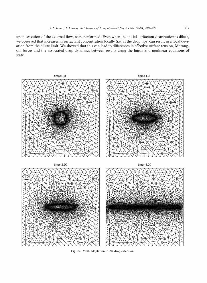
A.J. James, J. Lowengrub / Journal of Computational Physics 201 (2004) 685–722 717
upon cessation of the external flow, were performed. Even when the initial surfactant distribution is dilute,
we observed that increases in surfactant concentration locally (i.e. at the drop tips) can result in a local devi-
ation from the dilute limit. We showed that this can lead to differences in effective surface tension, Marang-
oni forces and the associated drop dynamics between results using the linear and nonlinear equations of
state.
Fig. 29. Mesh adaptation in 2D drop extension.
718 A.J. James, J. Lowengrub / Journal of Computational Physics 201 (2004) 685–722
There are numerous flow configurations we will simulate in the future, and several of these problems will
be used to compare our results to experiments. Comparison is difficult since the total amount of surfactant
on the interface generally cannot be measured, much less the surfactant distribution. However, our simu-
lations can be used to determine such quantities a posteriori by finding the parameters needed to match
experimental results. Such results can be very useful to the experimentalist. For example, we will comparethe velocity of a bubble rising under buoyancy, with and without surfactant, to experimental data. By
matching the bubble velocity, we will then likely be able to predict the actual surfactant coverage and dis-
tribution in the experiment. In particular, we will simulate experiments by Zhang and Finch [69] which re-
port the velocity of a buoyant bubble as a function of distance traveled after being released from rest for
three surfactant concentrations and two bubble sizes. In another problem of interest, Hu et al. [70] quantify
the deformation of a drop subjected to an extensional flow as a function of the capillary number and the
average surface tension. They vary the surface tension by varying surfactant concentration. Thus, by
matching the drop deformation in this experiment, we will also be able to predict the actual surfactant cov-erage and distribution along the drop.
There are several directions we will pursue in the future. To resolve the wide-ranging length and time
scales inherent in interfacial flows with surfactants, we will implement adaptive mesh refinement. This is
necessary to resolve, for example, very small secondary drops that may pinchoff from the ends of a
primary drop in the presence of surfactant (tip streaming). We will adapt the mesh refinement algo-
rithms developed by Zheng et al. [64] for level-set methods to a coupled level-set/volume-of-fluid meth-
od. In [64], a finite element implementation of the the level-set equations for low Reynolds number
interfacial flows (without surfactant) was solved using an unstructured, adaptive triangulated mesh in2D and an unstructured tetrahedral mesh in 3D. The mesh is adapted according to a node density
function [65] such that the density of nodes is highest near the interface. In preliminary work, we have
developed a 2D implementation of a coupled level-set/volume-of-fluid algorithm [66] for clean drops
and an example simulation of a drop in extensional flow using this new algorithm is shown in Fig.
29. Observe that the mesh is highly refined near the interface and tracks the evolution of the interface
throughout the domain.
In additional future work, we will link the volume fraction and interface area advection routines to cre-
ate a higher-order, self-consistent interface reconstruction. We will also simulate the transport of solublesurfactant in the fluid bulk and transfer of surfactant between the bulk and the interface. Finally, the simu-
lations will be generalized to 3D.
Acknowledgements
The authors thank Mike Siegel and especially Vittorio Cristini for helpful discussions concerning this
work. The authors acknowledge the support of the Minnesota Supercomputer Institute and the Networkand Academic Computing Services (NACS) at the University of California, Irvine. The first author thanks
3M Corp. for partial support. The second author thanks the National Science Foundation, Division of
Mathematical Sciences and the Department of Energy, Basic Energy Sciences Division for partial support.
The authors thank the Institute for Mathematics and its Applications at the University of Minnesota for
hospitality.
Appendix A. Concentration evolution equation
In this appendix, we demonstrate that Eq. (5) for the surfactant concentration is equivalent to alternative
formulations for incompressible given, for example, in [5]. For incompressible fluids,
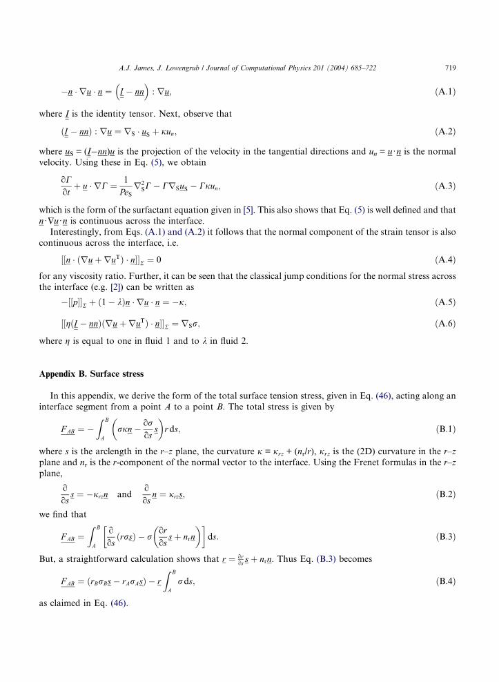
A.J. James, J. Lowengrub / Journal of Computational Physics 201 (2004) 685–722 719
�n � ru � n ¼ I � nn� �
: ru; ðA:1Þ
where I is the identity tensor. Next, observe that
ðI � nnÞ : ru ¼ rS � uS þ jun; ðA:2Þ
where uS = (I�nn)u is the projection of the velocity in the tangential directions and un = u Æn is the normalvelocity. Using these in Eq. (5), we obtain
oCot
þ u � rC ¼ 1
PeSr2
SC� CrSuS � Cjun; ðA:3Þ
which is the form of the surfactant equation given in [5]. This also shows that Eq. (5) is well defined and that
n Æ$u Æn is continuous across the interface.
Interestingly, from Eqs. (A.1) and (A.2) it follows that the normal component of the strain tensor is also
continuous across the interface, i.e.
½½n � ðruþruTÞ � n��R ¼ 0 ðA:4Þ
for any viscosity ratio. Further, it can be seen that the classical jump conditions for the normal stress acrossthe interface (e.g. [2]) can be written as
�½½p��R þ ð1� kÞn � ru � n ¼ �j; ðA:5Þ
½½gðI � nnÞðruþruTÞ � n��R ¼ rSr; ðA:6Þ
where g is equal to one in fluid 1 and to k in fluid 2.
Appendix B. Surface stress
In this appendix, we derive the form of the total surface tension stress, given in Eq. (46), acting along an
interface segment from a point A to a point B. The total stress is given by
F AB ¼ �Z B
Arjn� or
oss
� �rds; ðB:1Þ
where s is the arclength in the r–z plane, the curvature j = jrz + (nr/r), jrz is the (2D) curvature in the r–z
plane and nr is the r-component of the normal vector to the interface. Using the Frenet formulas in the r–z
plane,
o
oss ¼ �jrzn and
o
osn ¼ jrzs; ðB:2Þ
we find that
F AB ¼Z B
A
o
osðrrsÞ � r
oros
sþ nrn� �� �
ds: ðB:3Þ
But, a straightforward calculation shows that r ¼ oros sþ nrn. Thus Eq. (B.3) becomes
F AB ¼ ðrBrBs� rArAsÞ � rZ B
Ards; ðB:4Þ
as claimed in Eq. (46).
720 A.J. James, J. Lowengrub / Journal of Computational Physics 201 (2004) 685–722
References
[1] R.A. De Bruijn, Tipstreaming of drops in simple shear flows, Chem. Eng. Sci. 48 (1993) 277–284.
[2] R. Defay, I. Priogine, Surface Tension and Adsorption, Wiley, New York, 1966.
[3] D.I. Colliasand, R.K. Prudhomme, Diagnostic techniques of mixing effectiveness: the effect of shear and elongation in drop
production in mixing tanks, Chem. Eng. Sci. 47 (1992) 1401–1410.
[4] H.P. Grace, Dispersion phenomena in high viscosity immiscible fluid systems and application of static mixers as dispersion devices
in such systems, Chem. Eng. Commun. 14 (1982) 225–277.
[5] H.A. Stone, A simple derivation of the time-dependent convective–diffusion equation for surfactant transport along a deforming
interface, Phys. Fluids A 2 (1990) 111.
[6] H. Wong, D. Rumschitzki, C. Maldarelli, On the surfactant mass balance at a deforming fluid interface, Phys. Fluids 8 (1996)
3203–3204.
[7] H.A. Stone, L.G. Leal, The effects of surfactants on drop deformation and breakup, J. Fluid Mech. 222 (1990) 161–186.
[8] W.J. Milliken, H.A. Stone, L.G. Leal, The effect of surfactant on transient motion of Newtonian drops, Phys. Fluids A 5 (1993)
69–79.
[9] Y. Pawar, K.J. Stebe, Marangoni effects on drop deformation in an extensional flow: the role of surfactant physical chemistry. I.
Insoluble surfactants, Phys. Fluids 8 (1996) 1738–1751.
[10] C.D. Eggleton, Y.P. Pawar, K.J. Stebe, Insoluble surfactants on a drop in an extensional flow: a generalization of the stagnated
surface limit to deforming interfaces, J. Fluid Mech. 385 (1999) 79–99.
[11] C.D. Eggleton, T.-M. Tsai, K.J. Stebe, Tip streaming from a drop in the presence of surfactants, Phys. Rev. Lett. 87 (2001)
048302.
[12] X. Li, C. Pozrikidis, The effect of surfactants on drop deformation and on the rheology of dilute emulsions in Stokes flow, J. Fluid
Mech. 341 (1997) 165–194.
[13] S. Yon, C. Pozrikidis, A finite-volume/boundary-element method for flow past interfaces in the presence of surfactants, with
application to shear flow past a viscous drop, Comput. Fluids 27 (1998) 879–902.
[14] W.J. Milliken, L.G. Leal, The influence of surfactant on the deformation and breakup of a viscous drop: the effect of surfactant
solubility, J. Colloid Interface Sci. 166 (1994) 275–285.
[15] H. Zhou, V. Cristini, J. Lowengrub, C. W. Macosko, 3D adaptive finite-element simulations of deformable drops with soluble
surfactant: pair interactions and coalescence. Phys. Fluids, submitted.
[16] Y.-J. Jan, G. Tryggvason, Computational studies of contaminated bubbles, in: I. Sahin, G. Tryggvason (Eds.), Proceedings of a
Symposium on the Dynamics of Bubbles and Vorticity Near Free Surfaces, ASME, 1991, p. 46.
[17] H.D. Ceniceros, The effects of surfactants on the formation and evolution of capillary waves, Phys. Fluids 15 (2003) 245.
[18] J.U. Brackbill, D.B. Kothe, C. Zemach, A continuum method for modeling surface tension, J. Comput. Phys. 100 (1992) 335.
[19] J. Glimm, M.J. Graham, J. Grove, X.L. Li, T.M. Smith, D. Tan, F. Tangerman, Q. Zhang, Front tracking in two and three
dimensions, Comput. Math. Appl. 35 (1998) 1.
[20] G. Tryggvason, B. Bunner, A. Esmaeeli, D. Juric, N. Al-Rawahi, W. Tauber, J. Han, S. Nas, Y.J. Jan, A front tracking method
for the computations of multiphase flow, J. Comput. Phys. 169 (2001) 708.
[21] D.J. Torres, J.U. Brackbill, The point-set method: front tracking without connectivity, J. Comput. Phys. 165 (2000) 620.
[22] A. Shin, D. Juric, Modeling three-dimensional multiphase flow using a level contour reconstruction method for front tracking
without connectivity, J. Comput. Phys. 180 (2002) 427–470.
[23] S. Osher, R. Fedkiw, Level set methods: an overview and some recent results, J. Comput. Phys. 169 (2001) 463.
[24] M. Sussman, P. Smereka, S. Osher, A level-set approach for computing solutions to incompressible two-phase flow, J. Comput.
Phys. 114 (1994) 146.
[25] M. Sussman, A. Almgren, J. Bell, P. Colella, L. Howell, M. Welcome, An adaptive level set approach for incompressible two-
phase flows, J. Comput. Phys. 148 (1999) 81.
[26] Z. Li, R. Leveque, Immersed interface methods for Stokes flow with elastic boundaries or surface tension, SIAM J. Sci. Comput.
18 (1997) 709.
[27] L. Lee, R. Leveque, An immmersed interface method for incompressible Navier–Stokes equations, SIAM J. Sci. Comput. 25
(2003) 832.
[28] D. Jacqmin, Calculation of two-phase Navier–Stokes flows using phase-field modeling, J. Comput. Phys. 55 (1999) 96.
[29] D. Anderson, G.B. McFadden, A.A. Wheeler, Diffuse interface methods in fluid mechanics, Ann. Rev. Fluid Mech. 30 (1998) 139.
[30] H. Lee, J. Lowengrub, J. Goodman, Modeling pinchoff and reconnection in a Hele–Shaw cell: I. The models and their calibration,
Phys. Fluids 14 (2002) 492–513.
[31] H. Lee, J. Lowengrub, J. Goodman, Modeling pinchoff and reconnection in a Hele–Shaw cell: II. Analysis and simulation in the
nonlinear regime, Phys. Fluids 14 (2002) 514–545.
[32] M. Verschueren, F.N. van de Vosseand, H.E.H. Meijer, Diffuse-interface modeling of thermocapillary flow instabilities in a Hele–
Shaw cell, J. Fluid Mech. 434 (2001) 153.
A.J. James, J. Lowengrub / Journal of Computational Physics 201 (2004) 685–722 721
[33] J.-S Kim, K. Kang, J. Lowengrub, Conservative multigrid methods for Cahn–Hilliard fluids, J. Comput. Phys. 193 (2004) 511–
543.
[34] Y.Y. Renardy, M. Renardy, V. Cristini, A new volume-of-fluid formulation for surfactants and simulations of drop deformation
under shear at a low viscosity ratio, Eur. J. Mech. B 21 (2002) 49–59.
[35] A.J. James, M.K. Smith, A. Glezer, Vibration induced drop atomization and the numerical simulation of low-frequency single-
droplet ejection, J. Fluid Mech. 476 (2003) 29–62.
[36] M. Renardy, Y. Renardy, J. Li, Numerical simulation of moving contact line problems using a volume-of-fluid method, J.
Comput. Phys. 171 (2001) 243–263.
[37] R. Scardovelli, S. Zaleski, Direct numerical simulation of free surface and interfacial flow, Ann. Rev. Fluid Mech. 31 (1999)
576.
[38] J. Li, Y. Renardy, Numerical study of flows of two immiscible liquids at low Reynolds number, SIAM Rev. 42 (2000) 417–439.
[39] Y. Renardy, V. Cristini, Effect of inertia on drop breakup under shear, Phys. Fluids 13 (2001) 7–13.
[40] E.G. Puckett, A. Almgren, J. Bell, D.L. Marcus, W.G. Rider, A high-order projection method for tracking fluid interfaces in
variable density incompressible flows, J. Comput. Phys. 130 (1997) 269.
[41] Y. Renardy, M. Renardy, PROST: a parabolic reconstruction of surface tension for the volume-of-fluid method, J. Comput. Phys.
183 (2002) 400–421.
[42] C.W. Hirt, B.D. Nichols, Volume of fluid (VOF) method for the dynamics of free boundaries, J. Comput. Phys. 39 (1981) 201–
225.
[43] M. Sussman, E.G. Puckett, A coupled level-set and volume-of-fluid method for computing 3D and axisymmetric incompressible
two-phase flows, J. Comput. Phys. 162 (2000) 301–337.
[44] A. Bourlioux, A coupled level-set volume-of-fluid method for tracking material interfaces, in: Proceedings of the 6th Annual Int.
Symposium on Computational Fluid Dynamics, Lake Tahoe, CA, 1995.
[45] M. Sussman, A second order coupled level-set and volume-of-fluid method for computing growth and collapse of vapor bubbles,
J. Comput. Phys. 187 (2003) 110.
[46] R. Fedkiw, T. Aslam, B. Merriman, S. Osher, A nonoscillatory Eulerian approach to interfaces in multimaterials flows (the ghost
fluid method), J. Comput. Phys. 152 (1999) 423.
[47] H.S. Udaykumar, L. Tran, D.M. Belk, K.J. Vanden, An Eulerian method for computation of multimaterial impact with ENO
shock-capturing and sharp interfaces, J. Comput. Phys. 186 (2003) 136–177.
[48] T. Hou, Z. Li, S. Osher, H. Zhao, A hybrid method for moving interface problems with applications to Hele–Shaw flow, J.
Comput. Phys. 134 (1997) 457.
[49] B.T. Helenbrook, L. Martinelli, C.K. Law, A numerical method for solving incompressible flow problems with a surface of
discontinuity, J. Comput. Phys. 148 (1999) 366.
[50] G.P. Sasmal, J.I. Hochstein, Marangoni convection with a curved and deforming free surface in a cavity, J. Fluids Eng. 116 (1994)
557–582.
[51] M.A. Drumright-Clarke, Y. Renardy, The effect of insoluble surfactant at dilute concentration on drop breakup under shear with
inertia, Phys. Fluids 16 (2004) 14–21.
[52] J.-J. Xu, H.-K. Zhao, An Eularian formulation for solving partial differential equations along a moving interface, J. Sci. Comput.
19 (2003) 573–594.
[53] G.K. Batchelor, An Introduction to Fluid Dynamics, Cambridge University Press, New York, 1967.
[54] D.B. Kothe, R.C. Mjolsness, M.D. Torrey, RIPPLE: A computer program for incompressible flows with free surfaces, Los
Alamos National Lab Report LA-12007-MS, 1991.
[55] B.D. Nichols, C.W. Hirt, R.S. Hotchkiss, SOLA-VOF: A solution algorithm for transient fluid flow with multiple free boundaries,
Los Alamos National Lab Report LA-8355, 1980.
[56] R. Scardovelli, S. Zaleski, Direct numerical simulation of free-surface and interfacial flow, Ann. Rev. Fluid Mech. 31 (1999) 567–
603.
[57] F.H. Harlow, J.E. Welch, Numerical calculation of time-dependent viscous incompressible flow of fluid with free surface, Phys.
Fluids 8 (1965) 2182–2189.
[58] J.A. Meijerink, H.A. van der Vorst, Guidelines for the usage of incomplete decompositions in solving sets of linear equations as
they occur in practical problems, J. Comput. Phys. 44 (1981) 134–155.
[59] A.J. James, Vibration induced droplet ejection, Ph.D. Thesis, Georgia Institute of Technology, 2000.
[60] E.G. Puckett, A.S. Almgren, J.B. Bell, D.L. Marcus, W.J. Rider, A high-order projection method for tracking fluid interfaces in
variable density incompressible flows, J. Comput. Phys. 130 (1997) 269–282.
[61] D.B. Kothe, W.J. Rider, S.J. Mosso, J.S. Brock, J.I. Hochstein, Volume tracking of interfaces having surface tension in two and
three dimensions, in: Proceedings of the 34th Aerospace Sciences Meeting & Exhibit, January 15–18, 1996, Reno, NV, AIAA
Report 96-0859, 1996.
[62] A. James, J. Lowengrub, in preparation.
[63] M. Siegel, 2000, private communication.
722 A.J. James, J. Lowengrub / Journal of Computational Physics 201 (2004) 685–722
[64] V. Cristini, J. Lowengrub, Z. Zheng, A. Anderson, Adaptive remeshing algorithms for unstructured meshes: application to
interface capturing simulations of multiphase flows, J. Comput. Phys., submitted.
[65] V. Cristini, J. Blawzdziewicz, M. Loewenberg, An adaptive mesh algorithm for evolving surfaces: simulations of drop break-up
and coalescence, J. Comput. Phys. 169 (2001) 345–463.
[66] X. Yang, A. James, J. Lowengrub, X. Zheng, V. Cristini, An adaptive coupled level-set/volume-of-fluid method, in preparation.
[67] J. Li, Calcul d�interface affine par morceauz (piecewise linear interface calculation), C. R. Acad. Sci. Paris., Ser. IIb (Paris) 320
(1995) 391–396.
[68] R. Scardovelli, S. Zaleski, Interface reconstruction with least-square fit and split Eulerian–Lagrangian advection, Int. J. Numer.
Methods Fluids 41 (2003) 251–274.
[69] Y. Zhang, J.A. Finch, A note on single bubble motion in surfactant solutions, J. Fluid Mech. 429 (2001) 63–66.
[70] Y.T. Hu, D.J. Pine, L.G. Leal, Drop deformation, breakup, and coalescence with compatibilizer, Phys. Fluids 12 (2000) 484–489.