Embed Size (px)
Citation preview
AD-AI32 835 IMPLEMENTATION OF A SURORADIENT PROJECTION ALGORITHM 11 1/IIU) WISCONSIN UNIV-MADISON MATHEMATICS RESEARCH CENTERRW OWENS AUG 83 MRC-TSR-2550 0AA029-80-C-0041
UNCLASS CFLE F/G 12/1 NL
EIIIEEIIIIIIIDIIIIIIIIII 83
2.2-
132 12.L-
III2 1.4 jj 1.6
MICROCOPY RESOLUTION TEST CHART
NATIONAL BURLAU Of STANDARDS 19t4 A
Imhof""Of&mb Z.... ,
MRC Technical Summary Report # 2550
IMPLEMENTATION OF A SUBGRADIENTPROJECTION ALGORITHM II
Robert W. Owens
Mathematics Research CenterUniversity of Wisconsin-Madison610 Walnut StreetMadison, Wisconsin 53705
August 1983
(Received July 12, 1983)
Approved for public releaselITIl FILE COPY Distribution unlimited yT IOSponsored by SE£ F 1983U. S. Army Research
Office
P. 0. Box 12211Research Triangle Park LNorth Carloina 27709
83 092oio
UNIVERSITY OF WISCONSIN-MADISONMATHEMATICS RESEARCH CENTER
IMPLEMENTATION OF A SUBGRADIENTPPOJECTION ALGORITHM II
Robert W. Owens*
Technical Summary Report #2550August 1983KABSTRACT
This paper discusses the implementation of a subgradient projection
algorithm due to Sreedharan 11.rrfor the minimization, subject to a finite
number of smooth, convex constraints, of an objective function which is the
sum of a smooth, strictly convex function and a piecewise smooth convex
function. Computational experience with the algorithm on several test
problems and comparison of this experience with previously published results
is presented.
AMS (MOS) Subject Classification: 90C25, 65K05
Key Words: optimization, subgradient, convex function, algorithm
Work Unit Number 5 - Optimization and Large Scale Systems
C.R. Category: G.1.6
* Department of Mathematics, Lewis and Clark College, Portland, OR 97219USA.
Sponsored by the United States Army under Contract No. DAAG29-80-c-0041.
SIGNIFICANCE AND EXPLANATION
The need to optimize an objective function subject to some sort of
constraints arises in almost all fields that use mathematics. In many
problems, however, the objective function is not differentiable so that
standard algorithms based upon gradients are not applicable. This is the
case, for example, with many problems arising in economics and business, and
with certain design problems in engineering. One approach to addressing this
difficulty is to construct a suitable generalized gradient, the subgradient,
and base an algorithm upon it instead of on the gradient.
This paper discusses the implementation of a subgradient projection
algorithm for the minimization of a certain kind of non-differentiable,
nonlinear, convex function subject to a finite number of nonlinear, convex
constraints. Computational experience with the algorithm on several test
problems and comparison of this experience with previously published results
is presented.
Accessi.onFlor_N T S GT'- 31-YTIC T4B t_" % '
Justificantiot
By-Distribution/
Availability Codes
IAvail and/or
Dist I Special
The responsibility for the wording and views expressed in this descriptivesummary lies with MRC, and not with the author of this report.
IMPLEMENTATION OF A SU14RADIENTPROJECTION ALGORITHM II
Robert W. Owens*
1. Introduction
In the early 1960's, Rosen developed gradient projection algorithms for
nonlinear programming problems subject to linear (9] and nonlinear (10]
constraints. Recent work by Sreedharan has generalized this earlier work and
may be viewed as the subgradient counterpart of Rosen's work. In [123,
Sreedharan developed a subgradient projection algorithm for the minimization
of the sum of a piecewise-affine convex function and a smooth, strictly convex
function, subject to a finite number of linear constraints. Rubin [11]
reported on the implementation of that algorithm. Then in [13], Sreedharan
extended his previous results to the case of an objective function which is
the sum of a piecewise smooth convex function and a smooth, strictly convex
function, subject to a finite number of smooth, convex constraints. Parallel
to Rubin's investigations, this paper reports on the implementation of that
algorithm. Since this latter paper by Sreedharan is an extension and
generalization of the former, the computational results of Rubin are relevant
to this work; consequently, where reasonable, we have chosen to parallel
Rubin's presentation for ease of comparison of the results.
Considerable effort has been and continues to be expended minimizing
convex functions subject to convex constraints and the difficulties
encountered are numerous. While no implementable algorithm can successfully
Department of Mathematics, Lewis and Clark College, Portland, OR 97219USA.
Sponsored by the United States Army under Contract No. DAAG29-80-C-0041.
handle all problems, Breedharan's algorithm does address several which have
plagued others in the field. Rosen's original iterative algorithms were
susceptible to what is sometimes called jamming or zigzagging, i.e. the
generated sequence clustering at or converging to a nonoptimal point. Various
techniques have been proposed to avoid thist by using c-subgradients
Sreedharan's algorithm is guaranteed convergence to the optimal solution.
Others who have used c-subgradient projection methods, e.g. (31, encounter
computational difficulties since the complete e-subdifferential uses non local
information and its actual determination can be computationally prohibitive.
Sreedharan's algorithm requires that only a certain subset of the £-subdifferential
be computed, a more straightforward task. Polak's (7] gradient projection
algorithm essentially projects the gradient of the objective function onto
supporting tangent vector spaces, a method different than Sreedharan's. More-
over, Polak hypothesizes a certain linear independence of the gradients of the
C-binding constraints whereas the algorithm we are reporting on requires no
such assumption.
-2-
Ig
.9J
2. Problem
dLet Q C R be a nonempty, open, convex set, and let fo gi vji
iin,2...mJ-1,2,...,n be convex differentiable functions from
0 into R. Also, let f be strictly convex. Let x - (x e lg19(x) 4 0,
i=12,..,).We assume that X is bounded and satisfies Slater's constraint
qualification: there exists a e x such that gi(a) < 0, 1-1,2,....,If. Let
v(x) - max(v (x)fjI=,2,...,n). The problem to be solved, referred to as
problem (P) is:
minimize: f(x) + v(x)
(P):subject to: x e x
Vote that (P) has a unique solution since f + v is continuous and
strictly convex on the compact set X. Note also, however, that in general
f + v is not differentiable.
-3-
3. Notation
dGiven x, y e R , we denote the standard Euclidean inner product of x
and y by juxtapostion, i.e. xy, and the corresponding length of x is
denoted by lxi. Given a nonempty, closed convex set S C Rd , we denote by
N[S] the unique point of S of least norm. y = NIS] is the projection of
0 onto S and is characterized by the property that y(x-y) ) 0 for all
x e S. For a differentiable function *, denote by *'(x) the gradient of
at x. Given any set S C Rd , let cone S be the convex cone with apex
0 generated by S and cony S the convex hull of the set S.
For any point x e X and any C ) 0, define the following four sets:
I(x) = {itgi(x) ) -C 1 ( i ( ml
JC(x) = {jlv (x) ) v(x) -e, 1 C j 4 n)
C (x) = cone {glx)Ii e I (x))
KC(x) = conv {v;(x)Ij e Jclx)}.
With x e x, Io(X) is the set of active (i.e. binding) constraints at x,
while I C(x), with C > 0, is the set of £-active (i.e. almost binding)
constraints at x. JC(x), with E > 0 and x e X, is similarly interpreted
in terms of the maximizing functions that define the function v. C Cx) and£
K Cx) are the easily computable subsets of the c-subdifferentials referred
to in section 1.
-4-
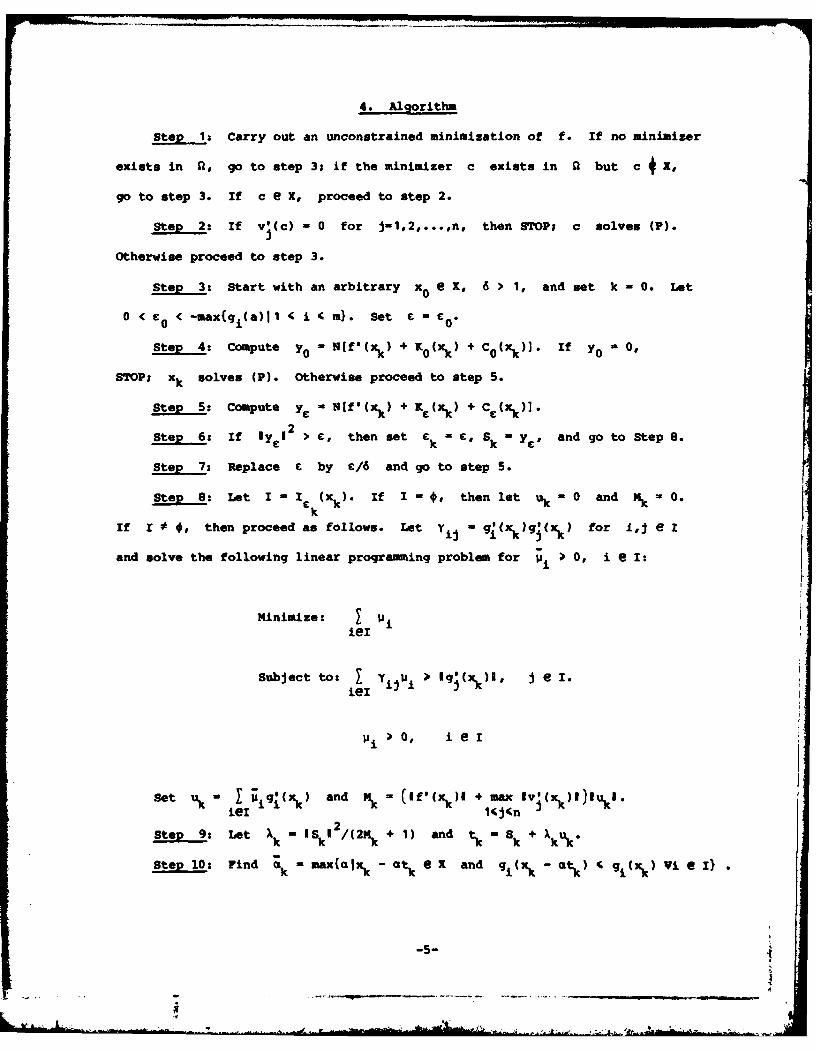
4. Algorithm
Step 1z Carry out an unconstrained minimization of f. If no minimizer
exists in a, go to step 31 if the minimizer c exists in 9 but c 4 X,
go to step 3. If c e X, proceed to step 2.
Step 2: If v;(c) - 0 for jal,2,...,n, then STOPI c solves (P).
Otherwise proceed to step 3.
Step 3: Start with an arbitrary x0 e x, 6 > I, and set k - 0. Let
0 < o < -maxgii(a)J1 - i - m). Set E - Co
Step 4: Compute y0 = N[f'(xk) + K0(xk ) + Co(xk)]. If Y0 - 0,
STOPi xk solves (P). Otherwise proceed to step 5.
Step 5: Compute y. W N[f'(xk) + KC(xk) + C (xk)]"12
Step 6: If ly > E, then set e k = E, S k y., and go to Step S.
Step 7: Replace E by E/6 and go to step 5.
Step 8: Let I - Ik (xk). If I - +, then let uk - 0 and Hk = O.
If I # *, then proceed as follows. Let y qi(xklgJ(x) for i,j e I
and solve the following linear programming problem for Vi 0 o, i e I:
Minimize:
ieI
Subject to: I Y )ji Ig;(x)i, J e I.ieI
Set gl- k) and -+wSet - a n - (lf'(X))l + max lv;(xk,)l)Iukl.
Step 9: Let Ak - 1Sk12/(2Kk + 1) and tk Sk + XkU k .
Step 10: Find -k max{aixk - et 6 X and gi(xk - a) g1 (xk) Vi 6 I}
-5-
... .. . ... -- ,-.... -.. .. . .. . .- - - ,,. ---. --;. . .. . . .: :J ,,':'" . . . . ._ ... _ _,.,
Stop 11: Find k e [O';k] such that there exists
zk e fl(x - aktk ) + KO(x - aktk ) with Zktk - O' If no such ak exists,
then set ak - ak*
Step 122 Set xk+ 1 - x - Cktk' increment k by 1, and go to step 4.
Steps 1 and 2 are present for technical reasons and rule out the
possibility that a given problem has an easily obtained solution. For many of
the test problems considered, these steps were bypassed since a specific
starting point was desired or it was known that a trivial solution did not
exist. In the fully implemented version of this algorithm actually tested,
step 1 was performed by calling the IMSL subroutine ZXCGR which employs a
conjugate gradient method to find the unconstrained minimum of an n variable
function of class C 1 .
The stopping criteria of either step 2 or step 4 would, in practice, be
replaced by ly 0 1 or 1vj (c) becoming sufficiently small.
In [13] it is shown that -tkI from step 9, is a feasible direction of
strict descent for f + v and that ak, from step 11, is strictly positive.
Before describing computational trials on test problems, the more
substantial subproblems involved in carrying out the steps of the given
algorithm are discussed. Specifically, we mention the projection problem
inherent in both steps 4 and 5, the linear programming problem of step 8, the
line search required in step 10, and the one dimensional minimization
indirectly called for in step 11.
-6-

5. Subproblems
The problem of computing the projection of 0 onto f'(x k ) + Kc(xk) + CE(x k )
with c - 0 (step 4) or e > 0 (step 5) is solved almost exactly as in [11],
i.e. the problem is expressed as a quadratic programming problem which is then
solved by standard techniques. For completeness we outline the key ideas; for
details see Rubin [1] and Cottle 14].
Assume that x e x, £ > o, :I(x)- (i 1 ... i) * *, and
J C(x) - (Jl,...,j) * #. y - Nff'(x) + K (x) + C (x)] can be written as
y fx) + kIIgk (x) + B v I )IkW, where Ok )0 0, k[l,
0 0, k -1,...,q, 0k 1, and (1/2)lf'(x) + x kg(kk-1
k
is a minimum over all such a and 0k s. Let hk = f(x) + v x),kk
k-1,...,q. Then f'(x) + B .iv' (x) - I Okh k Let e-k- k k-ik
be the p + q vector the first p of whose components are 0 and the last
q of whose components are 1. Let u = (a, .*."ap 0 '1... 8 q ),
M = ( g (x),...,gi (x), h 1,,..,h q), and Q = MTM, where the superscript T1 pq
denotes the transpose. The projection problem under consideration can now be
expressed as the quadratic programming problem:
Minimize: 1/2 uQu
Subject to: ue 1
u) 0
Rubin adapted an algorithm of Wolfe to solve this problem, an algorithm which
is guaranteed to terminate at the solution in finitely many steps. In the
present work, a package '11 develor d at the University of Wisconsin-Madison,
based on Cattle's version ". the principal pivoting method [4] was used.
-7-
Since the primary means of reporting on the success of the subgradient
projection algorithm is to give the number of iterations needed to obtain a
fixed accuracy, little extraordinary effort was expended optimizing the
computations involved in each iteration. Instead, IMSL subprograms were used
where convenient.
Step 8 requires the solution of the linear programming problem stated in
section 4; this problem is the dual of a standard linear programming problem
for which subroutine ZX3LP, a "revised simplex algorithm - easy to use
version,a is immediately applicable. No difficulties were encountered.
Step 10 involves a line search to locate ak" the maximum a such that
xk- atk e x and no previously £-binding constraint becomes more binding.
Letting
giC (x -
gi(G { - ttk) - g,(xk) i e I
and G(a) = max{G (a)11 4 i ( ml, and using the convexity of the gi, stepi
10 can be rephrased as: find the unique positive root ak of G(a) = 0.
After locating 0 < a < a such that G(aI) < 0 < G(a ), this latter
1 2 1 2
problem is solved by bisection with the stopping criteria being that
-12 -120 4 G() < 10 and Ja 1 - a2 1 < 10
- .
Step 11 requires that we locate, if it exists, ak e (O,k] such that
there exists zk e f'(xk - akt) + KO(x - aktk ) with zk tk = 0; if no such
ak exists, then set ak = 9k . This is equivalent to locating the minimum of
the strictly convex function F(c) - f(xk - atk) + v(xk - atk) on [0,ak] ;
see (13, Lemma 5.22]. The IMSL subroutine ZXGSP for one-dimensional unimodal
b-B-
function minimization using the Golden Section search method was used to solve
this subproblem. The stopping criterion employed was that the interval within
which the minimum occurs should be less than the minimum of 10 - 12 and
10 - 4 , . Occasionally an error message appeared saying that the function
did not appear unimodal to the subroutine; this was clearly due to roundoff
errors becoming significant. Nevertheless, these warnings posed no major
difficulties.
With the earlier, linear version of Sreedharan's algorithm, Rubin [11]
was able to carry out an efficient search for ak without explicitly locating
ak by exploiting the linearity of the gi and vj functions. Although
some improvement for finding a k in the present implementation is undoubtably
possible, no such dramatic economies are to be expected due to the
nonlinearity of the functions involved.
6. Computational Trials
The subqradient projection algorithm was implemented in Fortran 77 on a
VAX 11-780 using double precision (12-13 digits accuracy) and employing the
software described in section 5. For test purposes, 6 (step 3) was taken to
be 10. In order to avoid taking unnecessarily small steps early in a problem,
C was reset to Co at stop 4 for the first 4 iterations and was allowed to
follow the given nonincreasing pattern thereafter. The convergence criterion
of step 4 was relaxed to produce termination if either ly01 < 10- 12 or
Ix k - xk+I I < (1/2)o10 - 9 .
The first two problems below are ones considered by Rubin [11], neither
of which meet the hypothesis that f be strictly convex since in each
f-- 0.
Example 1. The first example was proposed by Wolfe [14] and uses d - 2,
f - 0, vI(X,y) - -x, v2(xy) - x + y, v3 (x,y) - x - 2y, n - 3. Following
Rubin, we investigated cases with constraints leading to a rectangular
feasible region having the global minimizer (0,0) of f + v interior to, on
the boundary of, and exterior to the feasible region. Table I summarizes the
results. The lower left and upper right corners of the feasible region are
given, as is the point at which the optimum value is achieved and the number
of iterations required to obtain termination. In each case
- -1/2 max gi(xoeyo).
The slow convergence occurs only, but not always, in cases where the
optimal solution is at a corner. The linear version of this algorithm was
able to handle all cases in at most 2 iterations [11].
-10-
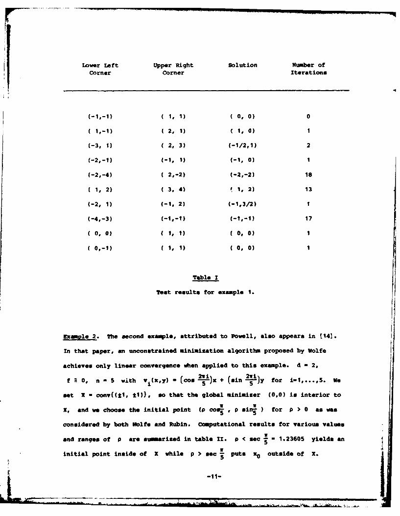
Lover Left Upper Right Solution Number ofCorner Corner Iterations
(-1 -1 ( 1, 1) 0 , 0) 0
( 1 -1 ( 2, 1) ( 1, O) 1
(-3, 1) C 2, 3) (-1/2,1) 2
(-2,-i) (-1, 1) (-1, 0) 1
(-2,-4) ( 2,-2) (-2,-2) 18
( 1, 2) ( 3, 4) I 1, 2) 13
(-2, 1) (-1, 2) (-1,3/2) 1
(-4,-3) (-1,-I) (-1,-i) 17
0 0, 0) 0 1, 1) ( 0, 0) 1
0,-1) ( 1, 1) 0 0, 0) 1
Table I
Tet results for example 1.
Example 2. The second example, attributed to Powell, also appears in [1.4].
In that paper, an unconstrained minimization algorithm proposed by Wolfe
achieves only linear convergence when applied to this example. d - 2,
f " 0, n - 5 with v (x,y) - Coos !I)x + (sin 2")y for w-1,...,5. We
set X - cony((1, t1)), so that the global minimizer (0,0) is interior to
X, and we choose the initial point (p cos. , P Simi ) for P > 0 as was
considered by both Wolfe and Rubin. Computational results for various valuesw
and ranges of p are sumarized in table I. p C sec -1 1.23605 yields an5
initial point inside of X while p > sec i puts x0 outside of X.5-
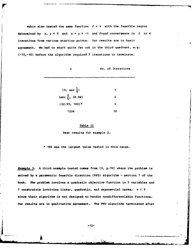
Rubin also tested the same function f + v with the feasible region
determined by x, y 4 0 and x + y 4 -1 and found convergence in 2 to 4
iterations from various starting points. Our results are in basic
agreement. We had to start quite far out in the third quadrant, e.g.
(-10,-10) before the algorithm required 5 iterations to terminate.
P No. of Iterations
[0, sec 7-) 15
(sec , 32.94) 2
(32.95, 100]* 3
1234 10
Table II
Test results for example 2.
* 100 was the largest value tested in this range.
Example 3. A third example tested comes from [2, p.76] where the problem is
solved by a parametric feasible direction (PFD) algorithm - section 7 of the
book. The problem involves a quadratic objective function in 5 variables and
7 constraints involving linear, quadratic, and exponential terms; v 0
since their algorithm is not designed to handle nondifferentiable functions.
Our resalts are in qualitative agreement. The PFD algorithm terminated after
-12-
ts , .
35 iterations with 6 decimal figures of accuracy; the subgradient projection
algorithm terminated after 41 iterations with 9 decimal figures of accuracy.
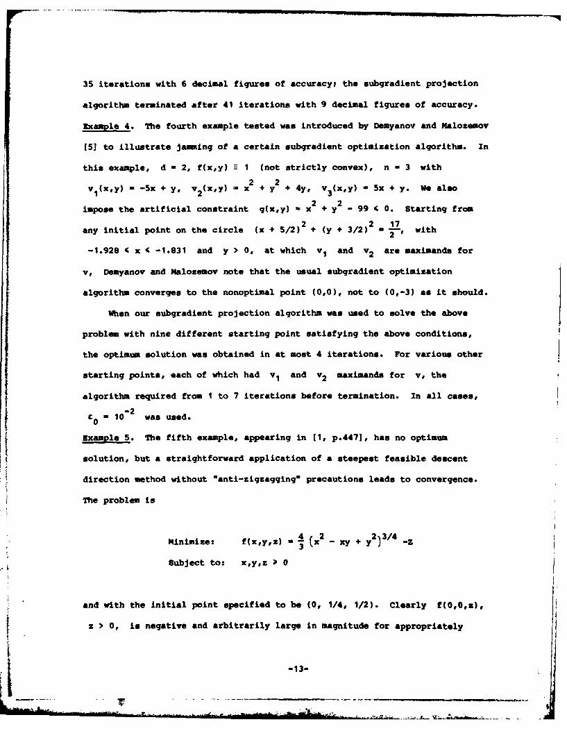
Example 4. The fourth example tested was introduced by Demyanov and Malozemov
(5] to illustrate jamming of a certain subgradient optimization algorithm. In
this example, d - 2, f(xy) 1 (not strictly convex), n - 3 with22
vl(xy) - -5x + y, v2(xY) x2 + y + 4y, v 3(xy) - 5x + y. We also
impose the artificial constraint g(xy) - x 2 + y2 _ 99 4 0. Starting from
2 2 17any initial point on the circle (x + 5/2) + (y + 3/2) = TO with
-1.928 4 x • -1.831 and y > 0, at which v1 and v2 are maximands for
v, Demyanov and Malozemov note that the usual subgradient optimization
algorithm converges to the nonoptimal point (0,0), not to (0,-3) as it should.
When our subgradient projection algorithm was used to solve the above
problem with nine different starting point satisfying the above conditions,
the optimum solution was obtained in at most 4 iterations. For various other
starting points, each of which had v1 and v2 maximands for v, the
algorithm required from I to 7 iterations before termination. In all cases,
-20 10 was used.
Example 5. The fifth example, appearing in (1, p.447], has no optimum
solution, but a straightforward application of a steepest feasible descent
direction method without "anti-zigzagging" precautions leads to convergence.
The problem is
Minimize: f(x,y,z) " (x2 - xy + y2 )3 /4 -Z
Subject to: x,yz ) 0
and with the initial point specified to be (0, 1/4, 1/2). Clearly f(0,O0,),
z > 0, is negative and arbitrarily large in magnitude for appropriately
-13-
-. -
chosen z. It is easily shown that, when the steepest feasible descent
direction method in employed, the iterates (xk, Yk' zk converge to
(0,0, v12: ith the third coordinate monotonically increasing. For test
2 2 2purposes, we introduced the extra, artificial constraint x + y +3 z 225
in order that the problem have a solution, albeit one very far removed from
the wfalse solution" to which the simpler algorithm converged. By k - 5 the
third coordinate had exceeded -j-,: by ki - 82 the artificial constraint was
binding; and the algorithm successfully terminated after III iterations.
Ixample 6. Finally the algorithm was tested on a family of problems each
involving two variables (d - 2), three vjs (n - 3), and four constraints
(m - 4). All functions were quadratic of the form a ICx-a 2 + a Ya4)2_ 5
and various trials were conducted with different choices of the parameters
ai. For example, consider the two problems with vICx,y) ( x-2)2 +
v2(x,y) - (1/2)(x 2 + y2 ), v3(x,y) x x2 + Cy-2 )2 ' gICx'y) -(x_1) 2 + Y2 - 4,
g2 (x~y) - (x+') 2 +. - 4, g3 (x,y) x2~ + (y_'1)2 _ 4, 94 (x,y) _ x2 + (y+1)2 - 4
With f~x,y) - (x-2) 2 + (y-2)2 the solution (a,a), - - J7- was found in
I step, while with f(x,y) - (x-4) 2 + (y-1) 2 the same optimum point was found
in 9 iterations. In each case Xo-(0,0) was obtained by the fully
implemented algorithm and co 1.5.
-14-
7. Conclusions
As Rubin (11] found with the earlier, linear version of this algorithm,
the subgradient projection algorithm is a viable method for solving a number
of convex programming problems including some which do not meet the hypotheses
needed to guarantee convergence, e.g. examples 1,2,4. When applied to smooth,
ie. differentiable, problems, e.g. example 3, it appears to perform competi-
tively with less general algorithms designed specifically to solve such
problems. It successfully avoids jamming on test problems that have been
specifically designed to jam, e.g. example 4. It qualitatively replicates the
results of the earlier linear method when applied to previously tested
problems. And it successfully solves in a small number of iterations larger
test problems designed to exercise the full range of capabilities built into
the algorithm.
Since one always wants faster convergence than is available, it might be
worth speculating on what factors might limit the performance of this
algorithm. The anti-jming techniques, although clearly necessary, seem to
entail a rather heavy cost in slowing down performance. Whereas the gradient
and even the subdifferential are local entities, the c-subdifferential is
not. While many £-subgradient based algorithms require knowledge of the
entire c-subdifferential, a formidable if not prohibitive task, Sreedharan'8
algorithm requires only an easily computable subset of that set. An appro-
priate element of the C-subdifferential is chosen and used to construct a
feasible direction of strict descent while avoiding jaming. One possible
source of difficulty is the difference between the directional derivative
F (x;u) and the C-subgradient based approximation to it, say F'(x;u),C
where F is the objective function, e.g. P - f + v in our case. Hiriart-
Urruty (61 has found that lF'(xlu) - ?(xiu)l - O(/e) as c.O. In some of
i-15-'
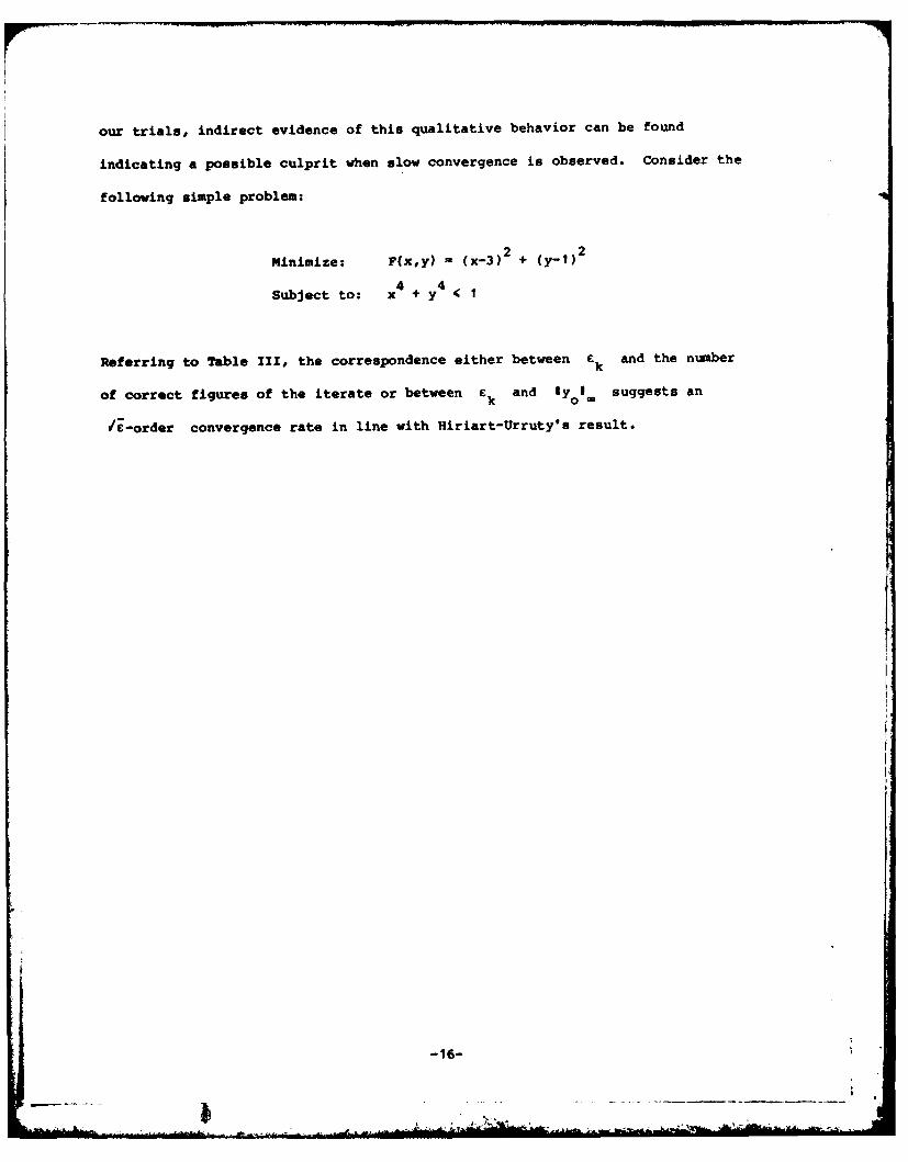
our trials, indirect evidence of this qualitative behavior can be found
indicating a possible culprit when slow convergence is observed. Consider the
following simple problem:
Minimize: F(x,y) - (x-3)2 + (y-1) 2
4 y4Subject to: x + 4<
Referring to Table III, the correspondence either between £k and the number
of correct figures of the iterate or between e k and lY o1 suggests an
ii-order convergence rate in line with Hiriart-Urruty's result.
-16-
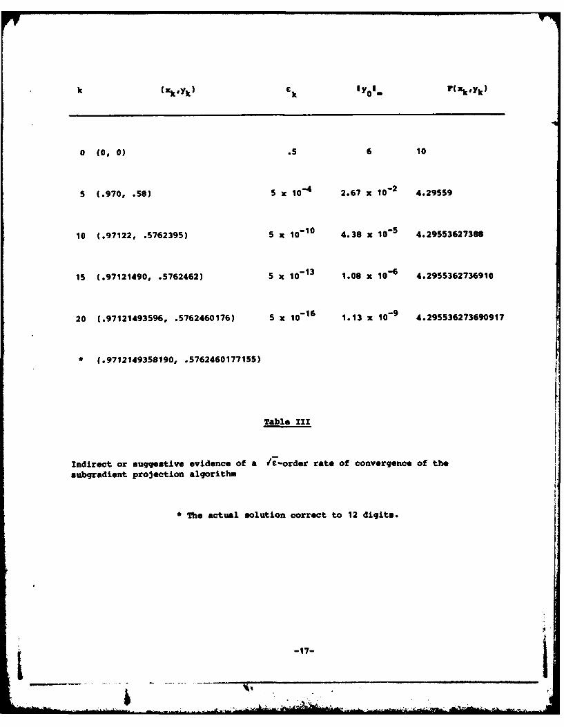
k (xkuyk) Ckl =rx~k
0 (0, 0) .5 6 10
5 (.970, .58) 5 x 0-4 2.67 x 10⁻² 4.29559
10 (.97122, .5762395) 5 x 10- 1 4.38 x 10⁵ 4.29553627388
15 (.97121490, .5762462) 5 x 10-13 1.08 x 1-6 4.2955362736910
20 (.97121493596, .5762460176) 5 x 10-16 1.13 x 10⁻⁹ 4.295536273690917
* (.9712149358190, .5762460177155)
Table III
Indirect or suggestive evidence of a IC-order rate of convergence of thesubqradient, projection algorithm
*The actual solution correct to 12 digits.
-17-
RZPXRNCRS
1. m. Avriel, "Nonlinear Programming& Analysis and Methods", Prentice-Hall,Inc., Englewood Cliffs., N.J., 1976.
2. A. Ben-Israel, A. Ben-Tal, and S. Zlobec, 0Optimality in Nonlinear
Programing: A Feasible Directions Approachs, John Wiley a Sons, New York,1981.
3. D. P. Bertsekas and S. K. Mitter, A descent numerical method foroptimization problems with nondifferentiable coast functionals, SIAM 3.Control 11 (1973), 4, 637-652.
4. R. W. Cottle, The principal pivoting method of quadratic programming,Mathematics of the Decision Sciences, 1 (1968), 144-162.
5. V. F. Demyanov and V. N. Malozemov, The theory of nonlinear minimax
problems, Uspekhi Mat. Nauk., 26 (1971), 53-104.
6. J.-B. Hiriart-Urrut~, e-subdifferential calculus, in "Convex Analysis and
Optimizationo, ed. by 3. P. Aubin and R. B. Vinter, Pitman, Research Notes
in Math., 57, London, 1982.
7. E. Polak, wComputational Methods in Optimization: A Unified Approachm,Academic Press, Ne York, 1971.
S. QUADMP/QUADPR, Academic Computing Center, University of Wisconsin-Madison,
1981.
9. 3. B. Rosen, The gradient projection method for nonlinear programming,Part It Linear constraints. 3. SIAM 8 (1960), 181-217.
10. 3. B. Rosen, The gradient projection method for nonlinear programming,
Part In: Nonlinear constraints, 3. SIAM 9 (1961), 514-532.
11. P. A. Rubin, Implementation of a subgradient projection algorithm, Inter.3. Computer Maths. 12 (1983), 321-328.
12. V. P. Sreedharan, A subgradient projection algorithm, 3. Approx. Theory 35
(1982), 2, 111-126.
13. V. P. Sreedharan, Another subgradient projection algorithm, to appear.
14. P. Wolfe, A method of conjugate subqradients for minimizing
nondifferentiable functions, Math. Prog. Study 3 (1975), 145-173.
UWO/jik
~-18-
SECURITY CLASSIFICATION OF THIS PAGE (I fte Data E toR D
REPORT DOCUMENTATION PAGE READ INSTRUCTOS-. REPORT NUMBER 2. GOVT ACCESSION NO. S. RECIPIENT*S CATALOG NUMBER
2550 ____________________1-_
4. TITLE (amd Subtitle) S. TYPE OF REPORT A PERIOD COVERED
Summary Report - no specificIMPLEMENTATION OF A SUBGRADIENT reporting periodPROJECTION ALGORITHM I I rprigpro6. PERFORMING ORG. REPORT NUMBER
7. AUTHOR(q) $. CONTRACT OR GRANT NUMBER(a)
Robert W. Owens DAAG9-80-C-0041
9. PERFORMING ORGANIZATION NAME AND ADDRESS 10. PROGRAM ELEMENT. PROJECT. TASKAREA • WORK UNIT NUMBERS
Mathematics Research Center, University of Work Unit Number 5 -610 Walnut Street Wisconsin Optimization and Large ScaleMadison, Wisconsin 53706 systems
II. CONTROLLING OFFICE NAME AND ADDRESS 12. REPORT DATE
U. S. Army Research Office August 1983
P.O. Box 12211 IS. NUMBER OF PAGES
Research Triangle Park. North Carolina 27709 1814. MONITORING 4GENCY NAME & ADDRESS(If direntahem Controlin Office) IS. SECURITY CLASS. (o We report)
UNCLASSIFIEDIS". OECLASSIFICATION/DOWN GRADI NG
SCHEDULE
IS. DISTRIBUTION STATEMENT (oftal Rep ")
Approved for public release; distribution unlimited.
17. DISTRISUTION STATEMENT (of t abetrac entred In Block 20, It difeent k Report)
I&. SUPPLEMENTARY NOTES
19. KEY WORDS (Coneme a revree aide It moeeeoay md IdontU by block number)
optimization, subgradient, convex function, algorithm
20. ABSTRACT rContinue on reverse side If neoceemy and identi by block momber)
This paper discusses the implementation of a subgradient projectionalgorithm due to Sreedharan [13] for the minimization, subject to a finitenumber of smooth, convex constraints, of an objective function which is thesum of a smooth, strictly convex function and a piecewise smooth convexfunction. Computational experience with the algorithm on several testproblems and comparison of this experience with previously published resultsis presented.
oN7 1473 EDITION OP I NOV 1S OBSOLETEEN ,ITCA" UNCLASSIFIEDSECUR ITY CLASIFPICATION OF THIS PAGE (IMan Data RhteeQ
41)
ATE
LMED
TIC
OIL.


![AD-AO89 b35 WISCONSIN UNIV-MADISON MATHEMATICS RESEARCH ... · ad-ao89 b35 wisconsin univ-madison mathematics research center f/s 12/1 ... 1.37 notes 169 w ... rudin [1974])](https://img.pdfslide.net/doc/110x75/5ae4f4f57f8b9a5b348f73bb/ad-ao89-b35-wisconsin-univ-madison-mathematics-research-b35-wisconsin-univ-madison.jpg)