1

A Survey of Geodetic Approaches to Mappingand the Relationship to Graph-Based SLAM

Pratik Agarwal1 Wolfram Burgard1 Cyrill Stachniss1,2

1 University of Freiburg, Institute of Computer Science, 79110 Freiburg, Germany2 University of Bonn, Institute of Geodesy and Geoinformation, 53115 Bonn, Germany

Abstract— The ability to simultaneously localize a robot andto build a map of the environment is central to most roboticapplications and the problem is often referred to as SLAM.Robotics researchers have proposed a large variety of solutionsallowing robots to build maps and use them for navigation. Alsothe geodetic community addressed large-scale map building forcenturies, computing maps which span across continents. Theselarge-scale mapping processes had to deal with several challengesthat are similar to those of the robotics community. In this paper,we explain key geodetic map building methods that we believeare relevant for robot mapping. We also aim at providing ageodetic perspective on current state-of-the-art SLAM methodsand identifying similarities both in terms of challenges facedas well as in the solutions proposed by both communities. Thecentral goal of this paper is to connect both fields and to enablefuture synergies between them.

I. INTRODUCTION

The problem of simultaneously localization and map-ping (SLAM) is essential for several robotic applications inwhich the robot is required to autonomously navigate. A mo-bile robot needs a map of its environment to plan appropriatepaths towards a goal location. Furthermore, following theplanned paths in turn requires the robot to localize itself in itsmap. Many modern SLAM methods follow the graph-basedSLAM paradigm [1], [2], [3], [4]. In this approach, each poseof the robot or each landmark position is represented as a nodein a graph. A constraint between two nodes, which results fromobservations, is represented by an edge in the graph. The firstpart of the overall problem is to create the graph, based onsensor data and such a system is often referred to as the front-end. The second part deals with finding the configuration of thenodes that best explains the constraints modeled by the edges.This step corresponds to computing the most-likely map (orthe distribution over possible maps) and a system solving it istypically referred to as a back-end.

In the geodetic mapping community, one major goal hasbeen to build massive survey maps, some even spanning acrosscontinents. These maps were supposed then be used eitherdirectly by humans or for studying large scale properties ofthe earth. In principle, geodetic maps are built in a similarway to the front-end/back-end approach used in SLAM. Con-straints are acquired through observations between physicalobservation towers. These towers correspond to positions ofthe robot as well as the landmarks in the context of SLAM.Once the constraints between observation towers are obtained,the goal is to optimize the resulting system of equations to get

the best possible locations of the towers on the surface of theearth.

The aim of this paper is to survey key approaches of thegeodetic mapping community and put them in relation torecent SLAM research. This mainly relates to the back-endsof graph-based SLAM systems. We believe that this step willenable further collaborations and exchanges among both fields.As we will illustrate during this survey, both communitieshave come up with sophisticated approximations to the fullleast squares approach for computing maps with the aimof reducing memory and computational resources. A centralstarting point for the survey of the geodetic approaches is the“North American Datum of 1983” by Charles R.Schwarz [5]and we go back to the work by Helmert [6] published in 1880.This paper extends [7] and presents a comprehensive reviewof the geodetic mapping techniques that we believe are relatedto SLAM.

In the remainder of this paper, we first identify the keysimilarities between the challenges faced in geodetic androbotic mapping. Second, we introduce graph-based SLAMand provide a short overview on it. Third, we explain theproblem formulation for geodetic mapping and introducecommonly used terminologies. We continue to explain theapproaches to geodetic mapping including the motivation andinsights central to the developed solutions. We then highlightthe relationships between individual SLAM approaches andgeodetic solutions.

II. COMMON CHALLENGES INGEODETIC AND ROBOTIC MAPPING

SLAM and geodetic mapping have several problems incommon. The first challenge is the large size of the maps.The map size in the underlying estimation problems is repre-sented by the number of unknowns. In geodetic mapping, theunknown are the positions of the observation towers, whilefor robotics, the unknowns corresponds to robot positions andobserved landmarks. For example, the system of equations forthe North American Datum of 1927 (NAD 27) required solvingfor 25,000 tower positions and the North American Datum of1983 (NAD 83) required solving for 270,000 positions [8].The largest real-world SLAM datasets have up to 21,000poses [9], while simulated datasets with 100,000 poses [10]and 200,000 poses [4] have been used for evaluation. At thetime of NAD 27 and 83, the map building problems could not

2

be solved by standard least squares methods as no computerwas capable to handle such large problems. Even nowadays,computational constraints are challenging in robotics. SLAMalgorithms often need to run on real mobile robots, includingbattery-powered wheeled platforms, small flying robots, andlow-powered underwater vehicles. For autonomous operation,the memory and computational requirements are often con-strained so that approximate but online algorithms are oftenpreferred over more precise but offline ones.

The second challenge results from outliers or spuriousmeasurements. The front-ends for both, robotics and geodeticmapping, are affected by outliers and noisy measurements. Inrobotics, the front-end is often unable to distinguish betweensimilar looking places, which leads to perceptual aliasing. Asingle outlier observation generated by the front-end can leadto a wrong solution, which in turn results in a map that isnot suitable to perform navigation tasks. To deal with thisproblem, there recently has been a more intense researchfor reducing the effect of outliers on the resulting map byusing extensions to the least squares approach [11], [12], [13],[14]. For geodetic mapping, the front-end consisted of humanscarefully and meticulously acquiring measurements. However,even this process was prone to making mistakes [5].

The third challenge comes from the non-linearity of con-straints, which is frequently the case in SLAM as wellas geodetic mapping. A commonly used approximation isto linearize the problem around an initial guess. However,this approximation to the non-linear problem may lead to asuboptimal solution if the initial guess is not in the basin ofconvergence. There are various methods, which enable findinga better initial guess, but this still remains a challenge [15],[16]. The importance of the initial guess in SLAM has alsomotivated the study of the convergence properties of thecorresponding nonlinear optimization problem [17], [18], [19],[20].

Fourth, both geodetic mapping and SLAM ideally requirean incremental and online optimization algorithm. In robotics,a robot is constantly building and using the map. It is ad-vantageous if the system is capable of optimizing the mapincrementally [21], [22]. In geodetic mapping, new surveytowers are build and new constraints are obtained as and whenrequired. It is not feasible to optimize the full network fromscratch when new areas or constraints are added. Thus, alsogeodetic methods must be able to incorporate new informationinto existing solutions with minimum computational demands.

Given these similarities, we believe that studying theachievements of the geodetic scholars is likely to inspire novelsolutions to large-scale, autonomous robotic SLAM.

III. GRAPH-BASED SLAM

In the robotics community, Lu and Milios [1] were thefirst who introduced a least squares-based direct method forSLAM. In their seminal paper, they propose the graph-basedframework in which each node models a robot pose andeach edge represents a constraint between the poses of therobot. These constraints can represent odometry measurementsbetween sequential robot poses produced by wheel encoders

and inertial measurement units or produced by sensor fusiontechniques such as scan matching [23], [24], [25], [26].

Graph-Based SLAM back-ends aim at finding the con-figuration of the nodes that minimize the error induced byconstraints. Let x = (x1, . . . , xn)T be the state vector wherexi describes the pose of node i. This pose xi is typicallythree-dimensional for a robot living in the 2D plane. Wecan describe the error function eij(x) for a single constraintbetween the nodes i and j as the difference between theobtained measurement zij and the expected measurementf(xi, xj) given the current state

eij(x) = f(xi, xj)− zij . (1)

The actual realization of the measurement function f de-pends on the sensor setup. For pose to pose constraints, onetypically uses the transformation between the poses. For poseto landmark constraints, we minimize the reprojection error ofthe observed landmark into the frame of the observing pose.The error minimization can be written as

x∗ = argminx

∑ij

eij(x)T Ωijeij(x), (2)

where Ωij is the information matrix associated to a constraintand x∗ is the optimal configuration of nodes with minimumsum of error induced by the edges. The solution to Eq. 2is based on successive linearization of the original non-linearcost typically around the current estimate. The non-linear errorfunction is linearized using Taylor series expansion around aninitial guess x:

eij(x + ∆x) ' eij(x) + Jij∆x, (3)

with the Jacobian

Jij =∂eij(x + ∆x)

∂∆x

∣∣∣∣∆x=0

. (4)

This leads to a quadratic form. In the end, the Jacobians fromall constraints can be stacked into a matrix and the minimumof the quadratic form can be found through direct methodssuch as Gauss-Newton, by solving the linear system

H∆x∗ = −b, (5)

where H =∑

ij JTijΩijJij and b =

∑ij J

TijΩijeij are the

elements of the quadratic form that results form the linearizederror terms and ∆x∗ is the increment to the nodes in the graphconfiguration that minimizes the error in the current iterationat the current linearization point:

x∗ = x + ∆x∗. (6)

As the measurements z and the poses x do not forman Euclidean space, it is advantageous to not subtract theexpected and obtained measurement in Eq. 1 but to performthe operations in a non-Euclidean manifold space [27], [28].This is especially helpful for constraints involving orientations.

In their seminal paper [1], Lu and Milios compute Eq. 5by inverting the quadratic matrix H . This is reported to bethe most computationally expensive operation as it scalescubic with the number of nodes. A lot of graph-based SLAMresearch focuses on efficiently solving Eq. 5 using domain

3

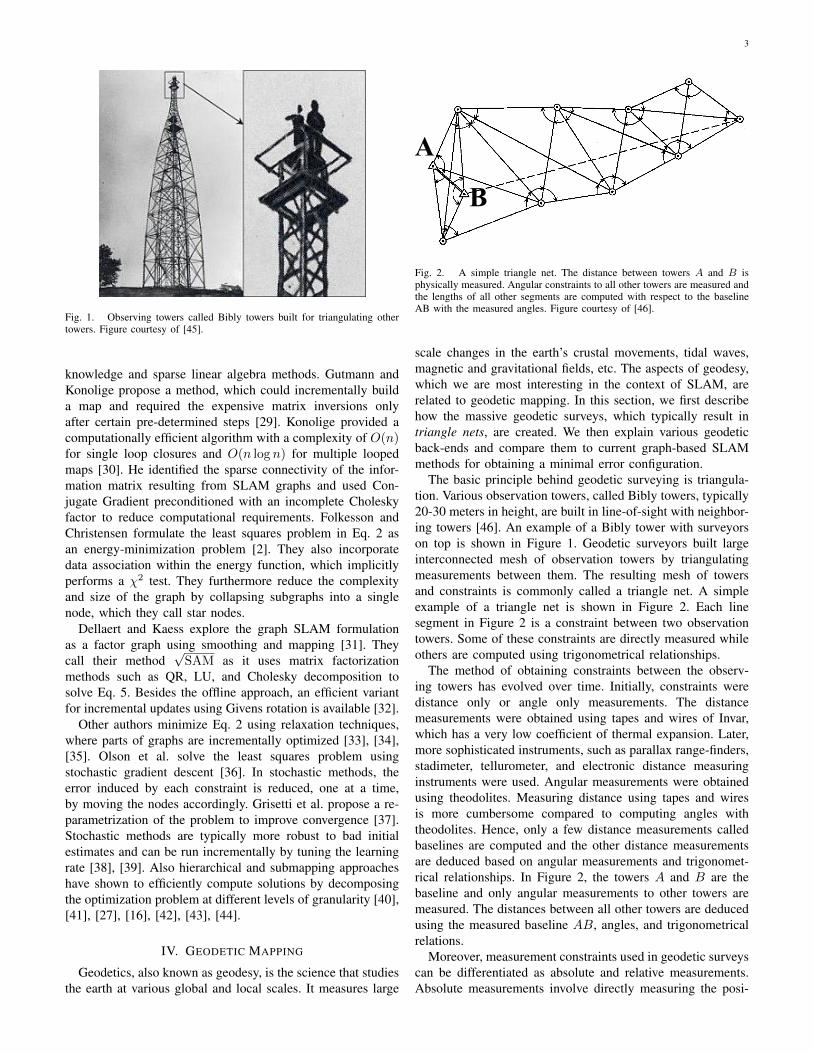
Fig. 1. Observing towers called Bibly towers built for triangulating othertowers. Figure courtesy of [45].

knowledge and sparse linear algebra methods. Gutmann andKonolige propose a method, which could incrementally builda map and required the expensive matrix inversions onlyafter certain pre-determined steps [29]. Konolige provided acomputationally efficient algorithm with a complexity of O(n)for single loop closures and O(n log n) for multiple loopedmaps [30]. He identified the sparse connectivity of the infor-mation matrix resulting from SLAM graphs and used Con-jugate Gradient preconditioned with an incomplete Choleskyfactor to reduce computational requirements. Folkesson andChristensen formulate the least squares problem in Eq. 2 asan energy-minimization problem [2]. They also incorporatedata association within the energy function, which implicitlyperforms a χ2 test. They furthermore reduce the complexityand size of the graph by collapsing subgraphs into a singlenode, which they call star nodes.

Dellaert and Kaess explore the graph SLAM formulationas a factor graph using smoothing and mapping [31]. Theycall their method

√SAM as it uses matrix factorization

methods such as QR, LU, and Cholesky decomposition tosolve Eq. 5. Besides the offline approach, an efficient variantfor incremental updates using Givens rotation is available [32].

Other authors minimize Eq. 2 using relaxation techniques,where parts of graphs are incrementally optimized [33], [34],[35]. Olson et al. solve the least squares problem usingstochastic gradient descent [36]. In stochastic methods, theerror induced by each constraint is reduced, one at a time,by moving the nodes accordingly. Grisetti et al. propose a re-parametrization of the problem to improve convergence [37].Stochastic methods are typically more robust to bad initialestimates and can be run incrementally by tuning the learningrate [38], [39]. Also hierarchical and submapping approacheshave shown to efficiently compute solutions by decomposingthe optimization problem at different levels of granularity [40],[41], [27], [16], [42], [43], [44].

IV. GEODETIC MAPPING

Geodetics, also known as geodesy, is the science that studiesthe earth at various global and local scales. It measures large

A

B

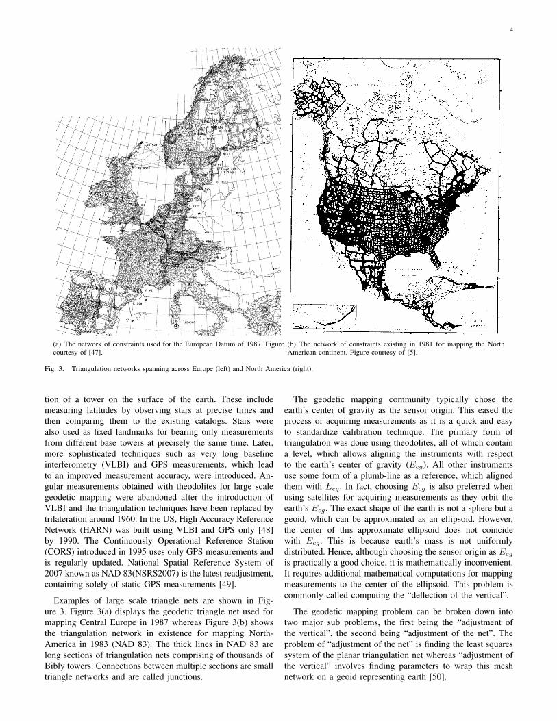
Fig. 2. A simple triangle net. The distance between towers A and B isphysically measured. Angular constraints to all other towers are measured andthe lengths of all other segments are computed with respect to the baselineAB with the measured angles. Figure courtesy of [46].

scale changes in the earth’s crustal movements, tidal waves,magnetic and gravitational fields, etc. The aspects of geodesy,which we are most interesting in the context of SLAM, arerelated to geodetic mapping. In this section, we first describehow the massive geodetic surveys, which typically result intriangle nets, are created. We then explain various geodeticback-ends and compare them to current graph-based SLAMmethods for obtaining a minimal error configuration.

The basic principle behind geodetic surveying is triangula-tion. Various observation towers, called Bibly towers, typically20-30 meters in height, are built in line-of-sight with neighbor-ing towers [46]. An example of a Bibly tower with surveyorson top is shown in Figure 1. Geodetic surveyors built largeinterconnected mesh of observation towers by triangulatingmeasurements between them. The resulting mesh of towersand constraints is commonly called a triangle net. A simpleexample of a triangle net is shown in Figure 2. Each linesegment in Figure 2 is a constraint between two observationtowers. Some of these constraints are directly measured whileothers are computed using trigonometrical relationships.

The method of obtaining constraints between the observ-ing towers has evolved over time. Initially, constraints weredistance only or angle only measurements. The distancemeasurements were obtained using tapes and wires of Invar,which has a very low coefficient of thermal expansion. Later,more sophisticated instruments, such as parallax range-finders,stadimeter, tellurometer, and electronic distance measuringinstruments were used. Angular measurements were obtainedusing theodolites. Measuring distance using tapes and wiresis more cumbersome compared to computing angles withtheodolites. Hence, only a few distance measurements calledbaselines are computed and the other distance measurementsare deduced based on angular measurements and trigonomet-rical relationships. In Figure 2, the towers A and B are thebaseline and only angular measurements to other towers aremeasured. The distances between all other towers are deducedusing the measured baseline AB, angles, and trigonometricalrelations.

Moreover, measurement constraints used in geodetic surveyscan be differentiated as absolute and relative measurements.Absolute measurements involve directly measuring the posi-

4

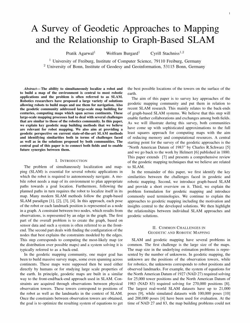
(a) The network of constraints used for the European Datum of 1987. Figurecourtesy of [47].

(b) The network of constraints existing in 1981 for mapping the NorthAmerican continent. Figure courtesy of [5].

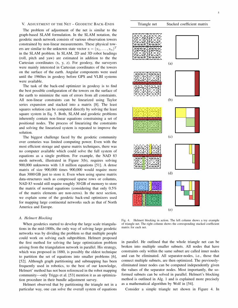
Fig. 3. Triangulation networks spanning across Europe (left) and North America (right).

tion of a tower on the surface of the earth. These includemeasuring latitudes by observing stars at precise times andthen comparing them to the existing catalogs. Stars werealso used as fixed landmarks for bearing only measurementsfrom different base towers at precisely the same time. Later,more sophisticated techniques such as very long baselineinterferometry (VLBI) and GPS measurements, which leadto an improved measurement accuracy, were introduced. An-gular measurements obtained with theodolites for large scalegeodetic mapping were abandoned after the introduction ofVLBI and the triangulation techniques have been replaced bytrilateration around 1960. In the US, High Accuracy ReferenceNetwork (HARN) was built using VLBI and GPS only [48]by 1990. The Continuously Operational Reference Station(CORS) introduced in 1995 uses only GPS measurements andis regularly updated. National Spatial Reference System of2007 known as NAD 83(NSRS2007) is the latest readjustment,containing solely of static GPS measurements [49].

Examples of large scale triangle nets are shown in Fig-ure 3. Figure 3(a) displays the geodetic triangle net used formapping Central Europe in 1987 whereas Figure 3(b) showsthe triangulation network in existence for mapping North-America in 1983 (NAD 83). The thick lines in NAD 83 arelong sections of triangulation nets comprising of thousands ofBibly towers. Connections between multiple sections are smalltriangle networks and are called junctions.

The geodetic mapping community typically chose theearth’s center of gravity as the sensor origin. This eased theprocess of acquiring measurements as it is a quick and easyto standardize calibration technique. The primary form oftriangulation was done using theodolites, all of which containa level, which allows aligning the instruments with respectto the earth’s center of gravity (Ecg). All other instrumentsuse some form of a plumb-line as a reference, which alignedthem with Ecg . In fact, choosing Ecg is also preferred whenusing satellites for acquiring measurements as they orbit theearth’s Ecg . The exact shape of the earth is not a sphere but ageoid, which can be approximated as an ellipsoid. However,the center of this approximate ellipsoid does not coincidewith Ecg . This is because earth’s mass is not uniformlydistributed. Hence, although choosing the sensor origin as Ecg

is practically a good choice, it is mathematically inconvenient.It requires additional mathematical computations for mappingmeasurements to the center of the ellipsoid. This problem iscommonly called computing the “deflection of the vertical”.

The geodetic mapping problem can be broken down intotwo major sub problems, the first being the “adjustment ofthe vertical”, the second being “adjustment of the net”. Theproblem of “adjustment of the net” is finding the least squaressystem of the planar triangulation net whereas “adjustment ofthe vertical” involves finding parameters to wrap this meshnetwork on a geoid representing earth [50].

5

V. ADJUSTMENT OF THE NET – GEODETIC BACK-ENDS

The problem of adjustment of the net is similar to thegraph-based SLAM formulation. In the SLAM notation, thegeodetic mesh network consists of various observation towersconstrained by non-linear measurements. These physical tow-ers are similar to the unknown state vector x = (x1, . . . , xn)T

in the SLAM problem. In SLAM, 2D and 3D robot headings(roll, pitch and yaw) are estimated in addition to the theCartesian coordinates (x, y, z). For geodesy, the surveyorswere mainly interested in Cartesian coordinates of the towerson the surface of the earth. Angular components were useduntil the 1960ies in geodesy before GPS and VLBI systemswere available.

The task of the back-end optimizer in geodesy is to findthe best possible configuration of the towers on the surface ofthe earth to minimize the sum of errors from all constraints.All non-linear constraints can be linearized using Taylorseries expansion and stacked into a matrix [8]. The leastsquares solution can be computed directly by solving the leastsquare system in Eq. 5. Both, SLAM and geodetic problemsinherently contain non-linear equations constraining a set ofpositional nodes. The process of linearizing the constraintsand solving the linearized system is repeated to improve thesolution.

The biggest challenge faced by the geodetic communityover centuries was limited computing power. Even with themost efficient storage and sparse matrix techniques, there wasno computer available which could solve the full system ofequations as a single problem. For example, the NAD 83mesh network, illustrated in Figure 3(b), requires solving900,000 unknowns with 1.8 million equations [51]. A densematrix of size 900,000 times 900,000 would require morethan 3000 GB just to store it. Even when using sparse matrixdata-structures such as compressed sparse rows or columns,NAD 83 would still require roughly 30 GB of memory to storethe matrix of normal equations (considering that only 0.5%of the matrix elements are non-zeros). In the next section,we explain some of the geodetic back-end optimizers usedfor mapping large continental networks such as that of NorthAmerica and Europe.

A. Helmert Blocking

When geodetics started to develop the large scale triangula-tions in the mid-1800s, the only way of solving large geodeticnetworks was by dividing the problem so that multiple peoplecould work on solving each subproblem. Helmert proposedthe first method for solving the large optimization problemarising from the triangulation network in parallel. His strategy,which was proposed in 1880, is possibly the oldest techniqueto partition the set of equations into smaller problems [6],[52]. Although graph partitioning and submapping has beenfrequently used in robotics, to the best of our knowledge,Helmert’ method has not been referenced in the robot mappingcommunity—only Triggs et al. [53] mention it as an optimiza-tion procedure in their bundle adjustment survey.

Helmert observed that by partitioning the triangle net in aparticular way, one can solve the overall system of equations

Triangle net Stacked coefficient matrix

(a)

(b)

(c)

(d)

(e)

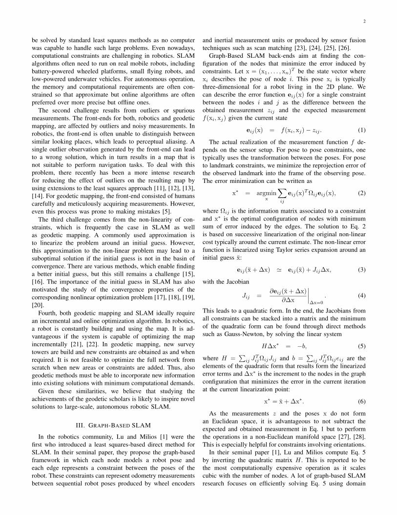
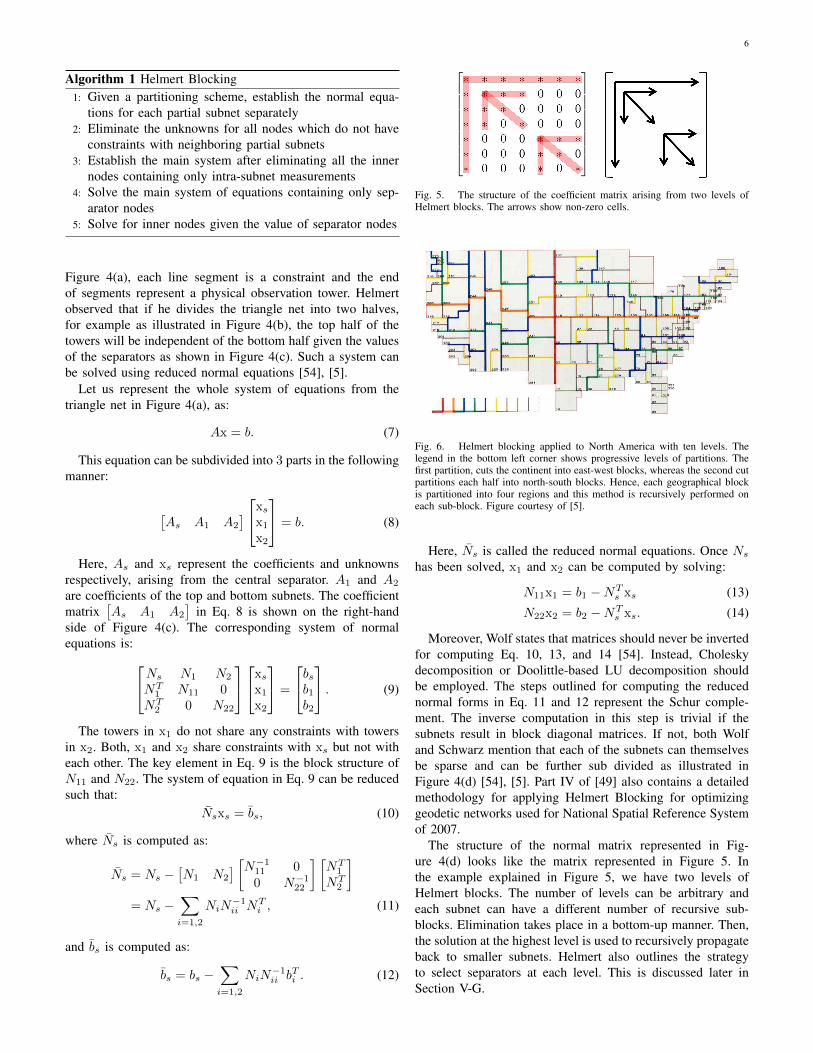
Fig. 4. Helmert blocking in action. The left column shows a toy exampleof triangle net. The right column shows the corresponding stacked coefficientmatrix for each net.

in parallel. He outlined that the whole triangle net can bebroken into multiple smaller subnets. All nodes that haveconstraints only within the same subnet are called inner nodesand can be eliminated. All separator-nodes, i.e., those thatconnect multiple subnets, are then optimized. The previously-eliminated inner nodes can be computed independently giventhe values of the separator nodes. Most importantly, the so-formed subnets can be solved in parallel. Helmert’s blockingmethod is outlined in Alg. 1 and is explained more preciselyas a mathematical algorithm by Wolf in [54].

Consider a simple triangle net shown in Figure 4. In

6

Algorithm 1 Helmert Blocking1: Given a partitioning scheme, establish the normal equa-

tions for each partial subnet separately2: Eliminate the unknowns for all nodes which do not have

constraints with neighboring partial subnets3: Establish the main system after eliminating all the inner

nodes containing only intra-subnet measurements4: Solve the main system of equations containing only sep-

arator nodes5: Solve for inner nodes given the value of separator nodes

Figure 4(a), each line segment is a constraint and the endof segments represent a physical observation tower. Helmertobserved that if he divides the triangle net into two halves,for example as illustrated in Figure 4(b), the top half of thetowers will be independent of the bottom half given the valuesof the separators as shown in Figure 4(c). Such a system canbe solved using reduced normal equations [54], [5].

Let us represent the whole system of equations from thetriangle net in Figure 4(a), as:

Ax = b. (7)

This equation can be subdivided into 3 parts in the followingmanner:

[As A1 A2

] xs

x1

x2

= b. (8)

Here, As and xs represent the coefficients and unknownsrespectively, arising from the central separator. A1 and A2

are coefficients of the top and bottom subnets. The coefficientmatrix

[As A1 A2

]in Eq. 8 is shown on the right-hand

side of Figure 4(c). The corresponding system of normalequations is:Ns N1 N2

NT1 N11 0

NT2 0 N22

xs

x1

x2

=

bsb1b2

. (9)

The towers in x1 do not share any constraints with towersin x2. Both, x1 and x2 share constraints with xs but not witheach other. The key element in Eq. 9 is the block structure ofN11 and N22. The system of equation in Eq. 9 can be reducedsuch that:

Nsxs = bs, (10)

where Ns is computed as:

Ns = Ns −[N1 N2

] [N−111 00 N−1

22

] [NT

1

NT2

]= Ns −

∑i=1,2

NiN−1ii N

Ti , (11)

and bs is computed as:

bs = bs −∑i=1,2

NiN−1ii b

Ti . (12)

Fig. 5. The structure of the coefficient matrix arising from two levels ofHelmert blocks. The arrows show non-zero cells.

Fig. 6. Helmert blocking applied to North America with ten levels. Thelegend in the bottom left corner shows progressive levels of partitions. Thefirst partition, cuts the continent into east-west blocks, whereas the second cutpartitions each half into north-south blocks. Hence, each geographical blockis partitioned into four regions and this method is recursively performed oneach sub-block. Figure courtesy of [5].

Here, Ns is called the reduced normal equations. Once Ns

has been solved, x1 and x2 can be computed by solving:

N11x1 = b1 −NTs xs (13)

N22x2 = b2 −NTs xs. (14)

Moreover, Wolf states that matrices should never be invertedfor computing Eq. 10, 13, and 14 [54]. Instead, Choleskydecomposition or Doolittle-based LU decomposition shouldbe employed. The steps outlined for computing the reducednormal forms in Eq. 11 and 12 represent the Schur comple-ment. The inverse computation in this step is trivial if thesubnets result in block diagonal matrices. If not, both Wolfand Schwarz mention that each of the subnets can themselvesbe sparse and can be further sub divided as illustrated inFigure 4(d) [54], [5]. Part IV of [49] also contains a detailedmethodology for applying Helmert Blocking for optimizinggeodetic networks used for National Spatial Reference Systemof 2007.

The structure of the normal matrix represented in Fig-ure 4(d) looks like the matrix represented in Figure 5. Inthe example explained in Figure 5, we have two levels ofHelmert blocks. The number of levels can be arbitrary andeach subnet can have a different number of recursive sub-blocks. Elimination takes place in a bottom-up manner. Then,the solution at the highest level is used to recursively propagateback to smaller subnets. Helmert also outlines the strategyto select separators at each level. This is discussed later inSection V-G.

7

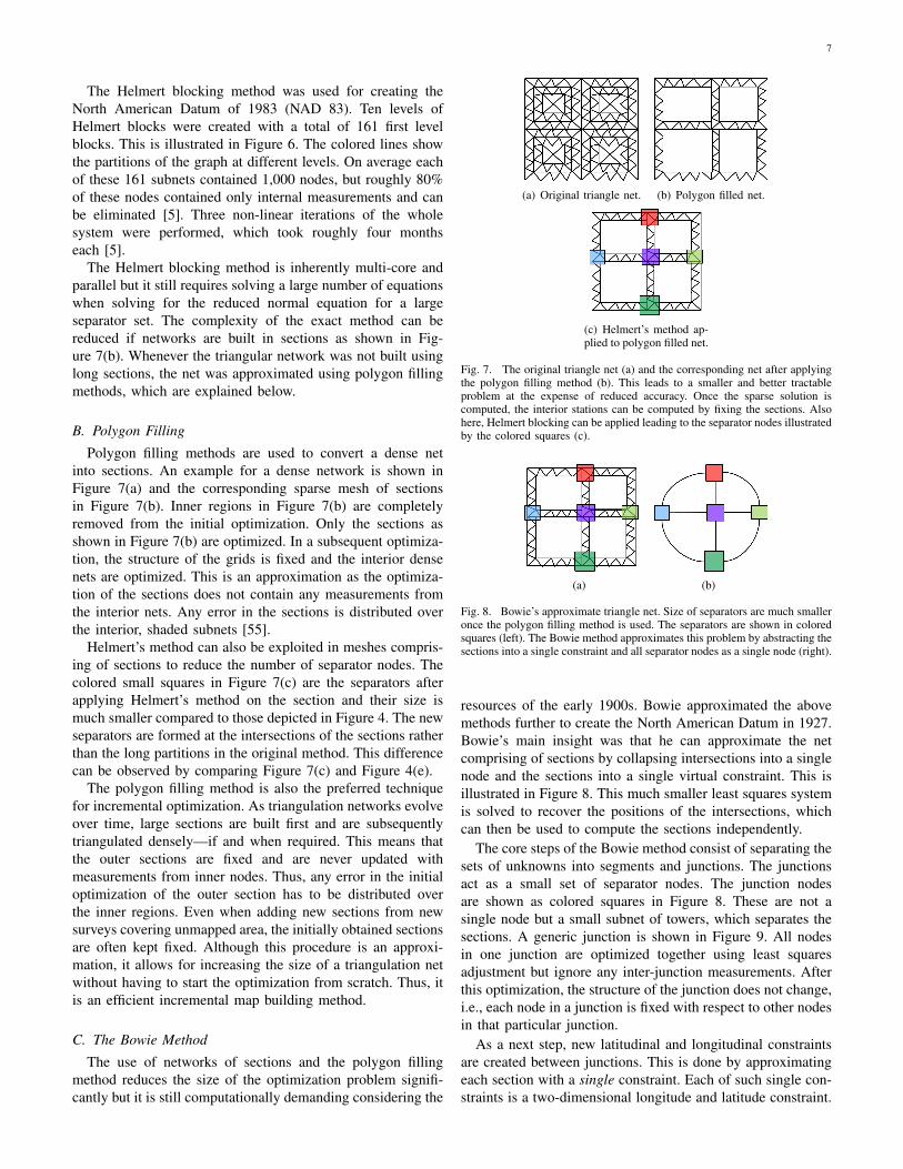
The Helmert blocking method was used for creating theNorth American Datum of 1983 (NAD 83). Ten levels ofHelmert blocks were created with a total of 161 first levelblocks. This is illustrated in Figure 6. The colored lines showthe partitions of the graph at different levels. On average eachof these 161 subnets contained 1,000 nodes, but roughly 80%of these nodes contained only internal measurements and canbe eliminated [5]. Three non-linear iterations of the wholesystem were performed, which took roughly four monthseach [5].

The Helmert blocking method is inherently multi-core andparallel but it still requires solving a large number of equationswhen solving for the reduced normal equation for a largeseparator set. The complexity of the exact method can bereduced if networks are built in sections as shown in Fig-ure 7(b). Whenever the triangular network was not built usinglong sections, the net was approximated using polygon fillingmethods, which are explained below.

B. Polygon Filling

Polygon filling methods are used to convert a dense netinto sections. An example for a dense network is shown inFigure 7(a) and the corresponding sparse mesh of sectionsin Figure 7(b). Inner regions in Figure 7(b) are completelyremoved from the initial optimization. Only the sections asshown in Figure 7(b) are optimized. In a subsequent optimiza-tion, the structure of the grids is fixed and the interior densenets are optimized. This is an approximation as the optimiza-tion of the sections does not contain any measurements fromthe interior nets. Any error in the sections is distributed overthe interior, shaded subnets [55].

Helmert’s method can also be exploited in meshes compris-ing of sections to reduce the number of separator nodes. Thecolored small squares in Figure 7(c) are the separators afterapplying Helmert’s method on the section and their size ismuch smaller compared to those depicted in Figure 4. The newseparators are formed at the intersections of the sections ratherthan the long partitions in the original method. This differencecan be observed by comparing Figure 7(c) and Figure 4(e).

The polygon filling method is also the preferred techniquefor incremental optimization. As triangulation networks evolveover time, large sections are built first and are subsequentlytriangulated densely—if and when required. This means thatthe outer sections are fixed and are never updated withmeasurements from inner nodes. Thus, any error in the initialoptimization of the outer section has to be distributed overthe inner regions. Even when adding new sections from newsurveys covering unmapped area, the initially obtained sectionsare often kept fixed. Although this procedure is an approxi-mation, it allows for increasing the size of a triangulation netwithout having to start the optimization from scratch. Thus, itis an efficient incremental map building method.

C. The Bowie Method

The use of networks of sections and the polygon fillingmethod reduces the size of the optimization problem signifi-cantly but it is still computationally demanding considering the

(a) Original triangle net. (b) Polygon filled net.

(c) Helmert’s method ap-plied to polygon filled net.

Fig. 7. The original triangle net (a) and the corresponding net after applyingthe polygon filling method (b). This leads to a smaller and better tractableproblem at the expense of reduced accuracy. Once the sparse solution iscomputed, the interior stations can be computed by fixing the sections. Alsohere, Helmert blocking can be applied leading to the separator nodes illustratedby the colored squares (c).

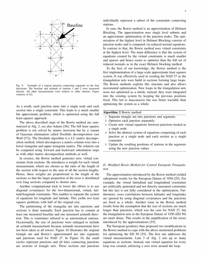
(a) (b)

Fig. 8. Bowie’s approximate triangle net. Size of separators are much smalleronce the polygon filling method is used. The separators are shown in coloredsquares (left). The Bowie method approximates this problem by abstracting thesections into a single constraint and all separator nodes as a single node (right).

resources of the early 1900s. Bowie approximated the abovemethods further to create the North American Datum in 1927.Bowie’s main insight was that he can approximate the netcomprising of sections by collapsing intersections into a singlenode and the sections into a single virtual constraint. This isillustrated in Figure 8. This much smaller least squares systemis solved to recover the positions of the intersections, whichcan then be used to compute the sections independently.

The core steps of the Bowie method consist of separating thesets of unknowns into segments and junctions. The junctionsact as a small set of separator nodes. The junction nodesare shown as colored squares in Figure 8. These are not asingle node but a small subnet of towers, which separates thesections. A generic junction is shown in Figure 9. All nodesin one junction are optimized together using least squaresadjustment but ignore any inter-junction measurements. Afterthis optimization, the structure of the junction does not change,i.e., each node in a junction is fixed with respect to other nodesin that particular junction.

As a next step, new latitudinal and longitudinal constraintsare created between junctions. This is done by approximatingeach section with a single constraint. Each of such single con-straints is a two-dimensional longitude and latitude constraint.

8

Baseline

Fig. 9. Example of a typical junction connecting segments in the fourdirections. The baseline and azimuth of stations 1 and 2 were measureddirectly. All other measurements were relative to other stations. Figurecourtesy of [5].

As a result, each junction turns into a single node and eachsection into a single constraint. This leads to a much smallerbut approximate problem, which is optimized using the fullleast-squares approach.

The above described steps of the Bowie method are sum-marized in Alg. 2, see also Adams [56]. The full least squaresproblem is not solved by matrix inversion but by a variantof Gaussian elimination called Doolittle decomposition (seeWolf [57]). The Doolittle algorithm is a LU matrix decompo-sition method, which decomposes a matrix column-wise into alower triangular and upper triangular matrix. The solution canbe computed using forward and backward substitution stepsas with other matrix decomposition methods as well.

In essence, the Bowie method generates new, virtual con-straints from sections. He introduces a weight for each virtualmeasurement, which are chosen as the ratio of the length ofthe section with respect to the sum of all the section lengths.Hence, these weights are proportional to the length of thesections so that the larger proportion of the error is distributedover long sections compared to shorter ones.

Another computational trick to lower the efforts is to usediagonal covariances for the two-dimensional, virtual, lati-tude/longitude constraints. This enables to separate the systemof equations for longitude and latitude. This yields two leastsquares problems with half of the original size.

The partitioning of the triangular net into junctions andsections is done manually. Each junction has to contain atleast one measured baseline and one measured azimuth direc-tion. This is sometimes referred to as astronomical stations.Occasionally, the size of junctions were enlarged to includean azimuth measurement because azimuth measurement havenot been taken at all towers. Figure 10 illustrates the originaltriangle net and Bowie’s approximated net into segmentsand junctions used for NAD 27. In Figure 10, the smallcircles represent junctions and all lines connecting junctionsare sections of triangle nets. These sections and junctions

individually represent a subset of the constraints connectingstations.

In sum, the Bowie method is an approximation of HelmertBlocking. The approximation uses single level subnets andan approximate optimization of the junction nodes. The opti-mization of the highest level in Helmert Blocking consists ofjunction nodes and is computed via reduced normal equations.In contrast to that, the Bowie method uses virtual constraintsat the highest level. The main difference is that the system ofequations created by the virtual constraints is much smallerand sparser and hence easier to optimize than the full set ofreduced normals as in the exact Helmert blocking method.

To the best of our knowledge, the Bowie method is thefirst implementation of a large scale approximate least squaressystem. It was effectively used in creating the NAD 27 as thetriangulation nets were build in sections forming large loops.The Bowie methods exploits this structure and also allowsincremental optimization. New loops in the triangulation netswere not optimized as a whole, instead, they were integratedinto the existing system by keeping the previous positionsfixed. This led to inaccuracies but was better tractable thanoptimizing the system as a whole.

Algorithm 2 Bowie method1: Separate triangle net into junctions and segments.2: Optimize each junction separately.3: Create new virtual equations between junctions treated as

a single node4: Solve the abstract system of equations comprising of each

junction as a single node and each section as a singleconstraint

5: Update the resulting positions of stations in the segmentsusing the new junction values

D. Modified Bowie Method for Central European Triangula-tion

The approximation introduced by the Bowie method yieldedsuboptimal results for the European Datum of 1950 [55]. Forexample, the virtual latitudinal and longitudinal constraintsare artificially generated and not directly measured constraintsbut this fact is not fully considered in the optimization. Fur-thermore, cross correlations between latitudes and longitudesare ignored by using diagonal covariances and the junctionsare fixed as a whole. Another issue in the Bowie methodresults from the assumption that the size of sections are muchlonger than junctions, which was the case for NAD 27, butthe triangulation nets in the European Datum of 1950 (ED 50)are more dense. This results in the amplification of the errorsintroduced by the approximations [55].

The European geodetics thus proposed two modifications tothe Bowie method to cope with the above mentioned problemsfor optimizing the ED 50 [55]. The first one addresses thevirtual measurements. Line 3 of Alg. 2 sets up as manyequations as sections. Instead, one virtual equation for everyloop was created, enforcing a zero error around the loop.

9

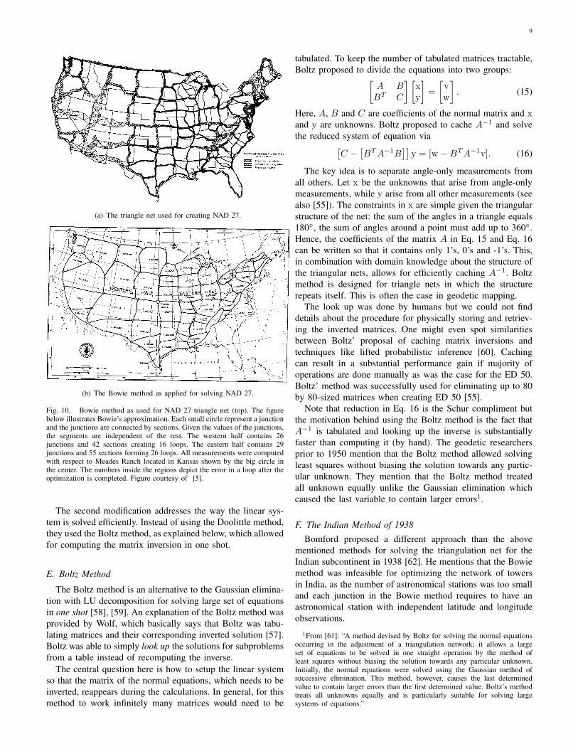
(a) The triangle net used for creating NAD 27.

(b) The Bowie method as applied for solving NAD 27.

Fig. 10. Bowie method as used for NAD 27 triangle net (top). The figurebelow illustrates Bowie’s approximation. Each small circle represent a junctionand the junctions are connected by sections. Given the values of the junctions,the segments are independent of the rest. The western half contains 26junctions and 42 sections creating 16 loops. The eastern half contains 29junctions and 55 sections forming 26 loops. All measurements were computedwith respect to Meades Ranch located in Kansas shown by the big circle inthe center. The numbers inside the regions depict the error in a loop after theoptimization is completed. Figure courtesy of [5].

The second modification addresses the way the linear sys-tem is solved efficiently. Instead of using the Doolittle method,they used the Boltz method, as explained below, which allowedfor computing the matrix inversion in one shot.

E. Boltz Method

The Boltz method is an alternative to the Gaussian elimina-tion with LU decomposition for solving large set of equationsin one shot [58], [59]. An explanation of the Boltz method wasprovided by Wolf, which basically says that Boltz was tabu-lating matrices and their corresponding inverted solution [57].Boltz was able to simply look up the solutions for subproblemsfrom a table instead of recomputing the inverse.

The central question here is how to setup the linear systemso that the matrix of the normal equations, which needs to beinverted, reappears during the calculations. In general, for thismethod to work infinitely many matrices would need to be

tabulated. To keep the number of tabulated matrices tractable,Boltz proposed to divide the equations into two groups:[

A BBT C

] [xy

]=

[vw

]. (15)

Here, A, B and C are coefficients of the normal matrix and xand y are unknowns. Boltz proposed to cache A−1 and solvethe reduced system of equation via[

C −[BTA−1B

]]y = [w −BTA−1v]. (16)

The key idea is to separate angle-only measurements fromall others. Let x be the unknowns that arise from angle-onlymeasurements, while y arise from all other measurements (seealso [55]). The constraints in x are simple given the triangularstructure of the net: the sum of the angles in a triangle equals180, the sum of angles around a point must add up to 360.Hence, the coefficients of the matrix A in Eq. 15 and Eq. 16can be written so that it contains only 1’s, 0’s and -1’s. This,in combination with domain knowledge about the structure ofthe triangular nets, allows for efficiently caching A−1. Boltzmethod is designed for triangle nets in which the structurerepeats itself. This is often the case in geodetic mapping.

The look up was done by humans but we could not finddetails about the procedure for physically storing and retriev-ing the inverted matrices. One might even spot similaritiesbetween Boltz’ proposal of caching matrix inversions andtechniques like lifted probabilistic inference [60]. Cachingcan result in a substantial performance gain if majority ofoperations are done manually as was the case for the ED 50.Boltz’ method was successfully used for eliminating up to 80by 80-sized matrices when creating ED 50 [55].

Note that reduction in Eq. 16 is the Schur compliment butthe motivation behind using the Boltz method is the fact thatA−1 is tabulated and looking up the inverse is substantiallyfaster than computing it (by hand). The geodetic researchersprior to 1950 mention that the Boltz method allowed solvingleast squares without biasing the solution towards any partic-ular unknown. They mention that the Boltz method treatedall unknown equally unlike the Gaussian elimination whichcaused the last variable to contain larger errors1.

F. The Indian Method of 1938

Bomford proposed a different approach than the abovementioned methods for solving the triangulation net for theIndian subcontinent in 1938 [62]. He mentions that the Bowiemethod was infeasible for optimizing the network of towersin India, as the number of astronomical stations was too smalland each junction in the Bowie method requires to have anastronomical station with independent latitude and longitudeobservations.

1From [61]: “A method devised by Boltz for solving the normal equationsoccurring in the adjustment of a triangulation network; it allows a largeset of equations to be solved in one straight operation by the method ofleast squares without biasing the solution towards any particular unknown.Initially, the normal equations were solved using the Gaussian method ofsuccessive elimination. This method, however, causes the last determinedvalue to contain larger errors than the first determined value. Boltz’s methodtreats all unknowns equally and is particularly suitable for solving largesystems of equations.”

10

(a) The mesh net with circuit errors on a zoomed section. (b) The resulting optimized net with the correction for eachjunction.

Fig. 12. A zoomed in view on the North-East section of the Indian subcontinent. It shows the initial and final configuration of the triangle net used in 1939for surveying India. The solid lines represent the initial spanning tree. The dotted lines are sections which induce circuit points and thus a residual error. Eachcircuit point contains the latitudinal residual error (top) and longitudinal residual error (bottom). Figure courtesy of [63].

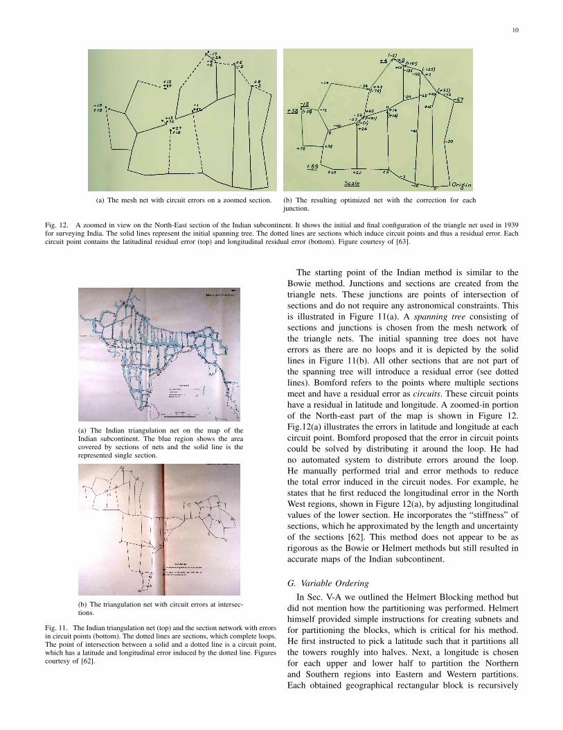
(a) The Indian triangulation net on the map of theIndian subcontinent. The blue region shows the areacovered by sections of nets and the solid line is therepresented single section.

(b) The triangulation net with circuit errors at intersec-tions.

Fig. 11. The Indian triangulation net (top) and the section network with errorsin circuit points (bottom). The dotted lines are sections, which complete loops.The point of intersection between a solid and a dotted line is a circuit point,which has a latitude and longitudinal error induced by the dotted line. Figurescourtesy of [62].

The starting point of the Indian method is similar to theBowie method. Junctions and sections are created from thetriangle nets. These junctions are points of intersection ofsections and do not require any astronomical constraints. Thisis illustrated in Figure 11(a). A spanning tree consisting ofsections and junctions is chosen from the mesh network ofthe triangle nets. The initial spanning tree does not haveerrors as there are no loops and it is depicted by the solidlines in Figure 11(b). All other sections that are not part ofthe spanning tree will introduce a residual error (see dottedlines). Bomford refers to the points where multiple sectionsmeet and have a residual error as circuits. These circuit pointshave a residual in latitude and longitude. A zoomed-in portionof the North-east part of the map is shown in Figure 12.Fig.12(a) illustrates the errors in latitude and longitude at eachcircuit point. Bomford proposed that the error in circuit pointscould be solved by distributing it around the loop. He hadno automated system to distribute errors around the loop.He manually performed trial and error methods to reducethe total error induced in the circuit nodes. For example, hestates that he first reduced the longitudinal error in the NorthWest regions, shown in Figure 12(a), by adjusting longitudinalvalues of the lower section. He incorporates the “stiffness” ofsections, which he approximated by the length and uncertaintyof the sections [62]. This method does not appear to be asrigorous as the Bowie or Helmert methods but still resulted inaccurate maps of the Indian subcontinent.

G. Variable Ordering

In Sec. V-A we outlined the Helmert Blocking method butdid not mention how the partitioning was performed. Helmerthimself provided simple instructions for creating subnets andfor partitioning the blocks, which is critical for his method.He first instructed to pick a latitude such that it partitions allthe towers roughly into halves. Next, a longitude is chosenfor each upper and lower half to partition the Northernand Southern regions into Eastern and Western partitions.Each obtained geographical rectangular block is recursively

11

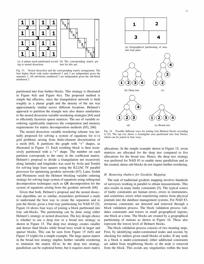
(a) A planar mesh partitioned accord-ing to nested dissection.

(b) The corresponding matrix pic-ture for this net.

Fig. 13. Nested dissection and the corresponding matrix arrangement. Thefour higher block with nodes numbered 1 and 2 are independent given theseparator 3. All sub-blocks numbered 1 are independent given the sub-blocknumbered 2.

partitioned into four further blocks. This strategy is illustratedin Figure 4(d) and Figure 4(e). The proposed method issimple but effective, since the triangulation network is builtroughly as a planar graph and the density of the net wasapproximately similar across different locations. Helmert’sapproach to partition the triangle nets also shares similaritiesto the nested dissection variable reordering strategies [64] usedto efficiently factorize sparse matrices. The use of variable re-ordering significantly improves the computation and memoryrequirements for matrix decomposition methods [65], [66].

The nested dissection variable reordering scheme was ini-tially proposed for solving a system of equations for n×ngrid problems arising from finite-element discretization ofa mesh [64]. It partitions the graph with “+” shapes, asillustrated in Figure 13. Each resulting block is then recur-sively partitioned with a “+” shape. The number on eachpartition corresponds to the entry in the coefficient matrix.Helmert’s proposal to divide a triangulation net recursivelyalong latitudes and longitudes was used by Avila and Tomlinfor solving large least squares using the ILLIAC IV parallelprocessor for optimizing geodetic networks [67]. Later, Goluband Plemmons used the Helmert blocking variable orderingstrategy for solving large system of equations using orthogonaldecomposition techniques such as QR decomposition for thesystem of equations arising from the geodetic network [68].

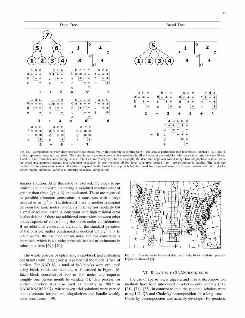
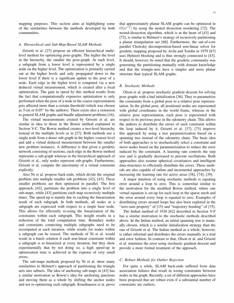
Given that both, Helmert’s proposal and the nested dissec-tion algorithm, are so similar, researchers performed a studyto understand the best way to create the separators and tojoin the blocks given a four-way partitioning for NAD 83 [5].Figure 14 shows four ways of joining a block partitioned intofour sub-blocks. The partitioning can be done using eitherHelmert’s strategy or nested dissection. The key design choiceis whether to use a deep tree or a broad tree strategy asshown in Figure 15. The deep tree strategy creates smallerand denser final blocks while broad trees result in larger andsparser blocks. This can be seen from Figure 15 (left) andFigure 15 (right) for a simple example. The large sparse matrixin the broad tree strategy implies further variable reorderingto minimize the matrix fill-in. In the deep tree strategy,parallelism can be exploited better, but it requires more matrix

(a) Geographical partitioning of areainto four parts

(b) Deep tree (c)

(d) (e) Broad tree

Fig. 14. Possible different ways for joining four Helmert blocks accordingto [5]. The top row shows a rectangular area partitioned into four blocks,which can be joined in four ways.

allocations. In the simple example shown in Figure 15, sevenmatrices are allocated for the deep tree compared to fiveallocations for the broad tree. Hence, the deep tree strategywas preferred for NAD 83 to enable more parallelism and asthe created, dense sub-blocks do not require further reordering.

H. Removing Outliers for Geodetic Mapping

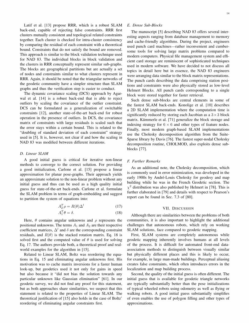
The task of traditional geodetic mapping involves hundredsof surveyors working in parallel to obtain measurements. Thisalso results in many faulty constraints [5]. The typical sourceof faulty constraints are human errors, errors in instruments,and sometimes errors when transferring entries from physicaljournals into the database management systems. For NAD 83,erroneous constraints are detected and removed through ablock validation process. The block validation process vali-dates constraints and towers in small geographical regions,one block at a time. The blocks are created by a geographicalpartitioning of stations as shown in Figure 16. These alsorepresent the lowest level of Helmert blocks.

The block validation process consists of two iterating steps.First, by identifying under-constrained nodes and second, bychecking for outliers given small blocks of nodes. If any nodein a block is under-constrained, either additional constraintsare added from neighboring blocks or the node is removedfrom the block. This avoids any singularities within the least

12

Deep Tree Broad Tree

ae

b

c

d

ae

b

c

d

* * ** *

*

abe

* * ** *

*

b c ebce

a b e

* * * ** * *

* * *

b a c ebace

* * ** *

*

ace

a c e

1 + 2 = 5' 5

* * ** *

*

ade

* * ** *

*

c d ecde

a d e

* * * ** * *

* * *

d a c edace

* * ** *

*

ace

a c e

3 + 4 = 6' 6

* * ** *

*

ace

* * ** *

*

a c eace

* * ** *

*

a d ea c eade

5 + 6 = 7

* * ** *

*

a b c d e

abe

* * ** *

*

b c ebce

* * ** *

*

a d e

abcde

* * ** *

*

c d ecde

* * * ** * * * *

* * * * *

*

a b eade

1 + 2 + 3 + 4

= 5

Fig. 15. Comparison between deep tree (left) and broad tree (right) ordering according to [5]. The area is partitioned into four blocks labeled 1, 2, 3 and 4.a to e represents separator variables. The variable set e are separators with constraints in all 4 blocks, a are variables with constraints only between blocks1 and 3, b are variables constraining between blocks 1 and 2 only, etc. In this example, the deep tree approach would merge two subgraphs at a time, whilethe broad tree approach merges four subgraphs at a time. In both methods all low level subgraphs labeled 1 to 4 are processed in parallel. The deep treemethod requires two more matrix allocation compared to the broad tree approach but the broad tree approach results in a larger matrix with zero blocks,which require additional variable re-ordering to reduce computation.

squares solution. After this issue is resolved, the block is op-timized and all constraints having a weighted residual error ofgreater than three (χ2 > 3) are evaluated. These are regardedas possible erroneous constraints. A constraint with a largeresidual error (χ2 > 3) is deleted if there is another constraintbetween the same nodes having a similar sensor modality buta smaller residual error. A constraint with high residual erroris also deleted if there are additional constraints between othernodes capable of constraining the nodes under consideration.If no additional constraints are found, the standard deviationof the possible outlier constrained is doubled until χ2 < 3. Inother words, the assumed sensor noise for this constraint isincreased, which is a similar principle behind m-estimators inrobust statistics [69], [70].

The whole process of optimizing a sub-block and evaluatingconstraints with large error is repeated till the block is free ofoutliers. For NAD 83, a total of 843 blocks were evaluatedusing block validation methods, as illustrated in Figure 16.Each block consisted of 300 to 500 nodes and requiredroughly one person month to validate [5]. This process foroutlier detection was also used as recently as 2007 forNAD83(NSRS2007), where seven trial solutions were carriedout to account for outliers, singularities and handle weaklydetermined areas [49].

Fig. 16. Boundaries of blocks of data used in the block validation process.Figure courtesy of [5].

VI. RELATION TO SLAM BACK-ENDS

The use of sparse linear algebra and matrix decompositionmethods have been introduced in robotics only recently [31],[21], [71], [22]. In contrast to that, the geodetic scholars wereusing LU, QR and Cholesky decomposition for a long time—Cholesky decomposition was actually developed for geodetic

13

mapping purposes. This section aims at highlighting someof the similarities between the methods developed by bothcommunities.

A. Hierarchical and Sub-Map-Based SLAM Methods

Grisetti et al. [27] propose an efficient hierarchical multi-level method for optimizing pose-graphs. The higher the levelin the hierarchy, the smaller the pose-graph. At each level,a subgraph from a lower level is represented by a singlenode on the higher level. The optimization is primarily carriedout at the higher levels and only propagated down to thelower level if there is a significant update to the pose of anode. Each edge in the higher level is computed via a newdeduced virtual measurement, which is created after a localoptimization. The gain in speed by this method results fromthe fact that computationally expensive optimization is onlyperformed when the pose of a node in the coarse representationgets affected more than a certain threshold (which was chosenas 5 cm or 0.05 by the authors). There exists also a extensionto general SLAM graphs and bundle adjustment problems [16].

The virtual measurements created by Grisetti et al. aresimilar in idea to those in the Bowie method explained inSection V-C. The Bowie method creates a two-level hierarchyinstead of the multiple levels as in [27]. Both methods use asingle node from a dense sub-graph in the higher, coarser leveland add a virtual deduced measurement between the smallernew problem instances. A difference is that given a geodeticnetwork consisting of sections, each edge in the Bowie methodrepresents a sub-graph whereas in the hierarchical approach ofGrisetti et al., only nodes represent sub-graphs. Furthermore,Grisetti et al. compute the uncertainty of a virtual constraintexplicitly.

Also Ni et al. propose back-ends, which divide the originalproblem into multiple smaller sub problems [42], [43]. Thesesmaller problems are then optimized in parallel. The firstapproach, [42], partitions the problem into a single level ofsub-maps, while [43] partitions each map recursively multipletimes. The speed-up is mainly due to caching the linearizationresult of each subgraph. In both methods, all nodes in asubgraph are expressed with respect to a single base node.This allows for efficiently re-using the linearization of theconstraints within each subgraph. This insight results in areduction of the total computation time. Boundary nodesand constraints connecting multiple subgraphs need to berecomputed at each iteration, while results for nodes withina subgraph can be reused. The methods of Ni et al. wouldresult in a batch solution if each non-linear constraint withina subgraph is re-linearized at every iteration, but they showexperimentally that by not doing so, a high speed-up inoptimization time is achieved at the expense of very smallerrors.

The sub-maps methods proposed by Ni et al. show manysimilarities to Helmert’s approach of partitioning the trianglenets into subnets. The idea of anchoring sub-maps in [43] hasa similar motivation as Bowie’s idea for anchoring junctionsand moving them as a whole by shifting the anchor nodesand not re-optimizing each subgraph. Krauthausen et at. prove

that approximately planar SLAM graphs can be optimized inO(n1.5) by using the nested dissection reordering [72]. Thenested-dissection algorithm, which is at the heart of [43] and[72], is similar to Helmert’s strategy of recursively partitioninga planar triangulation net [68]. Furthermore, the out-of-coreparallel Cholesky decomposition-based non-linear solver forgeodetic mapping proposed by Avila and Tomlin in 1979 [67]uses Helmert blocking and is thus strongly connected to [43].It should, however, be noted that the geodetic community wasgenerating the partitioning manually with domain knowledgeand that the triangle-nets have a simpler and more planarstructure than typical SLAM graphs.

B. Stochastic Methods

Olson et al. propose stochastic gradient descent for solvingpose-graphs with a bad initialization [36]. They re-parametrizethe constraints from a global pose to a relative pose represen-tation. In the global pose, all positional nodes are representedwith global coordinates in the world frame, whereas in therelative pose representation, each pose is represented withrespect to its previous pose in the odometry chain. This allowsthe authors to distribute the errors of each constraint withinthe loop induced by it. Grisetti et al. [37], [73] improvethis approach by using a tree parameterization based on aspanning tree instead of the odometry chain. The basic ideaof both approaches is to stochastically select a constraint andmove nodes based on the parameterization to reduce the errorinduced by the constraint. A learning rate controls the stepsize and is gradually decreased to prevent oscillations. Bothapproaches also assume spherical covariances and intelligentdata-structures to efficiently distribute the errors. These meth-ods are also capable of online and incremental approaches byincreasing the learning rate for active areas [38], [74], [39].

A major intuition of using stochastic methods is equatingerror around a loop to zero. This is somewhat similar tothe motivation for the modified Bowie method, where onevirtual equation is set-up for each loop in the sparse mesh andthe error around every loop is equated to zero. Examples ofdistributing errors around loops has also been explored in the“zero-sum property” of [15] and “trajectory bending” of [75].

The Indian method of 1938 [62] described in Section V-Fhas a similar motivation to the stochastic methods describedabove. In the Indian method, an initial spanning tree is manu-ally chosen, which is a similar initialization strategy than theone of Grisetti et al. The Indian method as a whole, however,is rather informal and distributes the errors manually in a trialand error fashion. In contrast to that, Olson et al. and Grisettiet al. minimize the error using stochastic gradient descent andprovide a more formal treatment of the approach.

C. Robust Methods for Outlier Rejection

For quite a while, SLAM back-ends suffered from dataassociation failures that result in wrong constraints betweennodes in the graph. Recently, a set of different approaches havebeen proposed that are robust even if a substantial number ofconstraints are outliers.

14

Latif et al. [13] propose RRR, which is a robust SLAMback-end, capable of rejecting false constraints. RRR firstclusters mutually consistent and topological related constraintstogether. Each cluster is checked for intra-cluster consistencyby comparing the residual of each constraint with a theoreticalbound. Constraints that do not satisfy the bound are removed.This approach is similar to the block validation technique usedfor NAD 83. The individual blocks in block validation andthe clusters in RRR conceptually represent similar sub-graphs.The blocks are geographical partitions but are actually a setof nodes and constraints similar to what clusters represent inRRR. Again, it should be noted that the triangular networks ofthe geodetic community have a simpler structure than SLAMgraphs and thus the verification step is easier to conduct.

The dynamic covariance scaling (DCS) approach by Agar-wal et al. [14] is a robust back-end that is able to rejectoutliers by scaling the covariance of the outlier constraint.DCS can be formulated as a generalization of switchableconstraints [12], another state-of-the-art back-end for robustoperation in the presence of outliers. In DCS, the covariancematrix of constraints with large residuals is scaled such thatthe error stays within a certain bound. This is related to the“doubling of standard deviation of each constraint” strategyused in [5]. It is, however, not clear if and how the scaling inNAD 83 was modified between different iterations.

D. Linear SLAM

A good initial guess is critical for iterative non-linearmethods to converge to the correct solution. For providinga good initialization, Carlone et al. [15] propose a linearapproximation for planar pose-graphs. Their approach yieldsan approximate solution to the non-linear problem without anyinitial guess and thus can be used as a high quality initialguess for state-of-the-art back-ends. Carlone et al. formulatethe SLAM problem in terms of graph-embedding and suggestto partition the system of equations into:

AT2 ρ = R(θ)∆l (17)

AT1 θ = δ. (18)

Here, θ contains angular unknowns and ρ represents thepositional unknowns. The terms A1 and A2 are their respectivecoefficient matrices, ∆l and δ are the corresponding constraintresiduals, and R(θ) is the stacked rotation matrix. Eq. 18 issolved first and the computed value of θ is used for solvingEq. 17. The authors provide both, a theoretical proof and real-world examples for the algorithm in [15].

Related to Linear SLAM, Boltz was reordering the equa-tions in Eq. 15 and eliminating angular unknowns first. Hismotivation was to cache matrix inversions for a faster humanlook-up, but geodetics used it not only for gains in speedbut also because it “did not bias the solution towards anyparticular unknown like Gaussian elimination” [61]. In ourgeodetic survey, we did not find any proof for this statement,but as both approaches share similarities, we suspect that thisstatement is related to the properties of Linear SLAM. Thetheoretical justification of [15] also holds in the case of Boltz’reordering of eliminating angular constraints first.

E. Dense Sub-Blocks

The manuscript [5] describing NAD 83 offers several inter-esting aspects ranging from database management to memoryand cache-friendly algorithms. During the project, engineersused punch card machines—rather inconvenient and cumber-some tools for solving large matrix problems compared tomodern computers. Physical file management system and effi-cient card storage are reminiscent of sophisticated techniquesused in modern software. We have decided to not discuss alltopics in detail here but in essence, the NAD 83 engineerswere arranging data similar to the block matrix representations.The punch cards describing the data comprising station posi-tions and constraints were also physically stored as low-levelHelmert Blocks. All punch cards corresponding to a singleblock were stored together for faster retrieval.

Such dense sub-blocks are central elements in some ofthe fastest SLAM back-ends. Konolige et al. [10] describesa 2D SLAM implementation where the computation time issignificantly reduced by storing each Jacobian as a 3×3 blockmatrix. Kummerle et al. [71] generalize the block storage andindexing strategy for 6 × 6 and other types of feature nodes.Finally, most modern graph-based SLAM implementationsuse the Cholesky decomposition algorithm from the Suite-Sparse library by Davis [76]. The fastest super-nodal Choleskydecomposition routine, CHOLMOD, also exploits dense sub-blocks [77].

F. Further Remarks

As an additional note, the Cholesky decomposition, whichis commonly used in error minimization, was developed in theearly 1900s by Andre-Louis Cholesky for geodesy and mapbuilding while he was in the French Geodetic section. Theχ2 distribution was also published by Helmert in [78]. This isfurther elaborated in [79] and details with respect to Pearson’sreport can be found in Sec. 7.3 of [80].

VII. DISCUSSION

Although there are similarities between the problems of bothcommunities, it is also important to highlight the additionalchallenges that autonomous robots, which rely on workingSLAM solutions, face compared to geodetic mapping.

First, SLAM systems are completely autonomous whilegeodetic mapping inherently involves humans at all levelsof the process. It is difficult for automated front-end data-association methods to distinguish between visually similarbut physically different places and this is likely to occur,for example, in large man-made buildings. Perceptual aliasingcreates false constraints, which often introduces errors in thelocalization and map building process.

Second, the quality of the initial guess is often different. Theinitial guess that is available for geodetic triangle networksare typically substantially better than the pose initializationsof typical wheeled robots using odometry as well as flying orwalking robots. A good initial guess substantially simplifiesof even enables the use of polygon filling and other types ofapproximations.

15

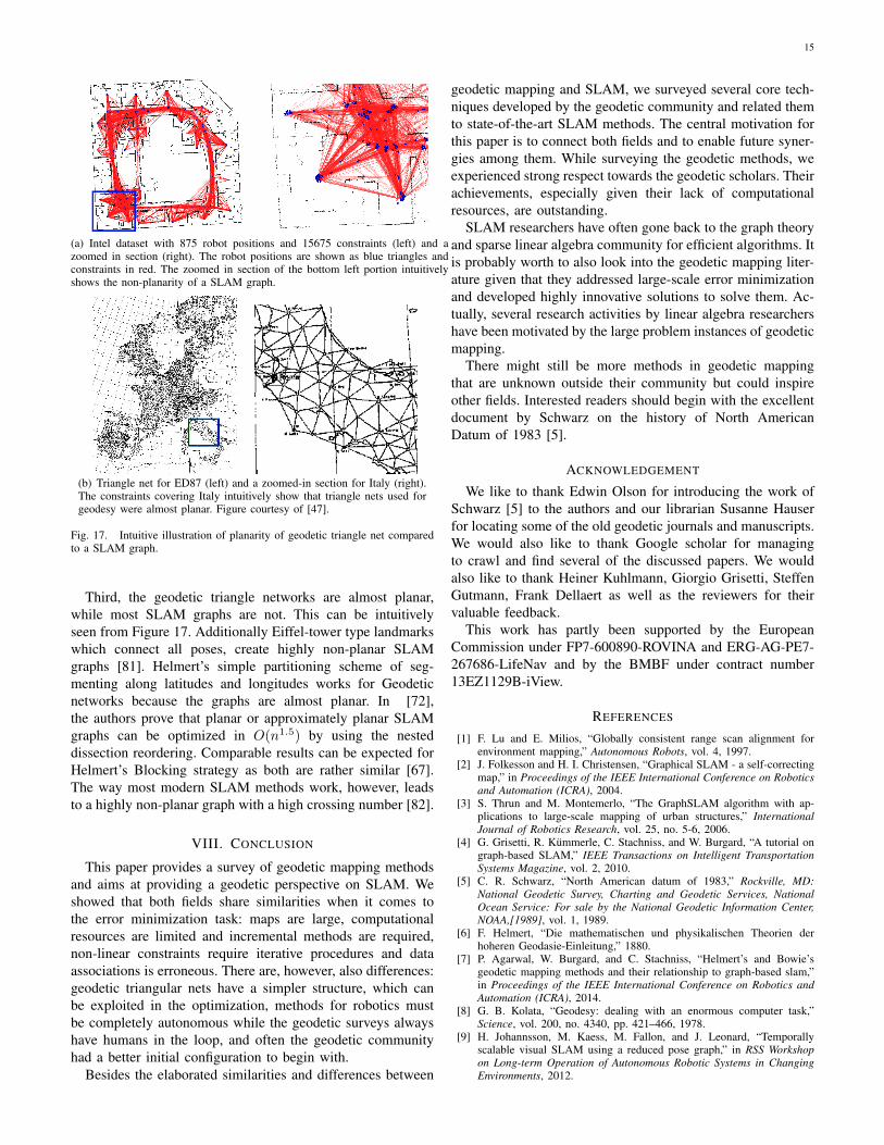
(a) Intel dataset with 875 robot positions and 15675 constraints (left) and azoomed in section (right). The robot positions are shown as blue triangles andconstraints in red. The zoomed in section of the bottom left portion intuitivelyshows the non-planarity of a SLAM graph.

(b) Triangle net for ED87 (left) and a zoomed-in section for Italy (right).The constraints covering Italy intuitively show that triangle nets used forgeodesy were almost planar. Figure courtesy of [47].

Fig. 17. Intuitive illustration of planarity of geodetic triangle net comparedto a SLAM graph.

Third, the geodetic triangle networks are almost planar,while most SLAM graphs are not. This can be intuitivelyseen from Figure 17. Additionally Eiffel-tower type landmarkswhich connect all poses, create highly non-planar SLAMgraphs [81]. Helmert’s simple partitioning scheme of seg-menting along latitudes and longitudes works for Geodeticnetworks because the graphs are almost planar. In [72],the authors prove that planar or approximately planar SLAMgraphs can be optimized in O(n1.5) by using the nesteddissection reordering. Comparable results can be expected forHelmert’s Blocking strategy as both are rather similar [67].The way most modern SLAM methods work, however, leadsto a highly non-planar graph with a high crossing number [82].

VIII. CONCLUSION

This paper provides a survey of geodetic mapping methodsand aims at providing a geodetic perspective on SLAM. Weshowed that both fields share similarities when it comes tothe error minimization task: maps are large, computationalresources are limited and incremental methods are required,non-linear constraints require iterative procedures and dataassociations is erroneous. There are, however, also differences:geodetic triangular nets have a simpler structure, which canbe exploited in the optimization, methods for robotics mustbe completely autonomous while the geodetic surveys alwayshave humans in the loop, and often the geodetic communityhad a better initial configuration to begin with.

Besides the elaborated similarities and differences between

geodetic mapping and SLAM, we surveyed several core tech-niques developed by the geodetic community and related themto state-of-the-art SLAM methods. The central motivation forthis paper is to connect both fields and to enable future syner-gies among them. While surveying the geodetic methods, weexperienced strong respect towards the geodetic scholars. Theirachievements, especially given their lack of computationalresources, are outstanding.

SLAM researchers have often gone back to the graph theoryand sparse linear algebra community for efficient algorithms. Itis probably worth to also look into the geodetic mapping liter-ature given that they addressed large-scale error minimizationand developed highly innovative solutions to solve them. Ac-tually, several research activities by linear algebra researchershave been motivated by the large problem instances of geodeticmapping.

There might still be more methods in geodetic mappingthat are unknown outside their community but could inspireother fields. Interested readers should begin with the excellentdocument by Schwarz on the history of North AmericanDatum of 1983 [5].

ACKNOWLEDGEMENT

We like to thank Edwin Olson for introducing the work ofSchwarz [5] to the authors and our librarian Susanne Hauserfor locating some of the old geodetic journals and manuscripts.We would also like to thank Google scholar for managingto crawl and find several of the discussed papers. We wouldalso like to thank Heiner Kuhlmann, Giorgio Grisetti, SteffenGutmann, Frank Dellaert as well as the reviewers for theirvaluable feedback.

This work has partly been supported by the EuropeanCommission under FP7-600890-ROVINA and ERG-AG-PE7-267686-LifeNav and by the BMBF under contract number13EZ1129B-iView.

REFERENCES

[1] F. Lu and E. Milios, “Globally consistent range scan alignment forenvironment mapping,” Autonomous Robots, vol. 4, 1997.

[2] J. Folkesson and H. I. Christensen, “Graphical SLAM - a self-correctingmap,” in Proceedings of the IEEE International Conference on Roboticsand Automation (ICRA), 2004.

[3] S. Thrun and M. Montemerlo, “The GraphSLAM algorithm with ap-plications to large-scale mapping of urban structures,” InternationalJournal of Robotics Research, vol. 25, no. 5-6, 2006.

[4] G. Grisetti, R. Kummerle, C. Stachniss, and W. Burgard, “A tutorial ongraph-based SLAM,” IEEE Transactions on Intelligent TransportationSystems Magazine, vol. 2, 2010.

[5] C. R. Schwarz, “North American datum of 1983,” Rockville, MD:National Geodetic Survey, Charting and Geodetic Services, NationalOcean Service: For sale by the National Geodetic Information Center,NOAA,[1989], vol. 1, 1989.

[6] F. Helmert, “Die mathematischen und physikalischen Theorien derhoheren Geodasie-Einleitung,” 1880.

[7] P. Agarwal, W. Burgard, and C. Stachniss, “Helmert’s and Bowie’sgeodetic mapping methods and their relationship to graph-based slam,”in Proceedings of the IEEE International Conference on Robotics andAutomation (ICRA), 2014.

[8] G. B. Kolata, “Geodesy: dealing with an enormous computer task,”Science, vol. 200, no. 4340, pp. 421–466, 1978.

[9] H. Johannsson, M. Kaess, M. Fallon, and J. Leonard, “Temporallyscalable visual SLAM using a reduced pose graph,” in RSS Workshopon Long-term Operation of Autonomous Robotic Systems in ChangingEnvironments, 2012.

16

[10] K. Konolige, G. Grisetti, R. Kummerle, W. Burgard, B. Limketkai,and R. Vincent, “Efficient sparse pose adjustment for 2d mapping,” inProceedings of the IEEE/RSJ International Conference on IntelligentRobots and Systems (IROS), 2010.

[11] E. Olson and P. Agarwal, “Inference on networks of mixtures for robustrobot mapping,” in Proceedings of Robotics: Science and Systems (RSS),2012.

[12] N. Sunderhauf and P. Protzel, “Towards a robust back-end for pose graphslam,” in Proceedings of the IEEE International Conference on Roboticsand Automation (ICRA), 2012.

[13] Y. Latif, C. C. Lerma, and J. Neira, “Robust loop closing over time,” inProceedings of Robotics: Science and Systems (RSS), 2012.

[14] P. Agarwal, G. D. Tipaldi, L. Spinello, C. Stachniss, and W. Bur-gard, “Robust map optimization using dynamic covariance scaling,”in Proceedings of the IEEE International Conference on Robotics andAutomation (ICRA), 2013.

[15] L. Carlone, R. Aragues, J. Castellanos, and B. Bona, “A linear ap-proximation for graph-based simultaneous localization and mapping,”in Proceedings of Robotics: Science and Systems (RSS), 2011.

[16] G. Grisetti, R. Kummerle, and K. Ni, “Robust optimization of factorgraphs by using condensed measurements,” in Proceedings of theIEEE/RSJ International Conference on Intelligent Robots and Systems(IROS), 2012.

[17] H. Wang, G. Hu, S. Huang, and G. Dissanayake, “On the structure ofnonlinearities in pose graph slam,” in Proceedings of Robotics: Scienceand Systems (RSS), 2012.

[18] L. Carlone, “A convergence analysis for pose graph optimization viagauss-newton methods,” in Proceedings of the IEEE International Con-ference on Robotics and Automation (ICRA). IEEE, 2013.

[19] G. Hu, K. Khosoussi, and S. Huang, “Towards a reliable slam back-end,”in Proceedings of the IEEE/RSJ International Conference on IntelligentRobots and Systems (IROS). IEEE, 2013, pp. 37–43.

[20] P. Agarwal, G. Grisetti, G. D. Tipaldi, L. Spinello, W. Burgard, andC. Stachniss, “Experimental analysis of dynamic covariance scaling forrobust map optimization under bad initial estimates,” in Proceedings ofthe IEEE International Conference on Robotics and Automation (ICRA),2014.

[21] M. Kaess, A. Ranganathan, and F. Dellaert, “Fast incremental square rootinformation smoothing,” in International Joint Conference on ArtificialIntelligence (IJCAI), 2007.

[22] M. Kaess, H. Johannsson, R. Roberts, V. Ila, J. Leonard, and F. Dellaert,“iSAM2: Incremental smoothing and mapping using the Bayes tree,”International Journal of Robotics Research, vol. 31, 2012.

[23] F. Lu and E. Milios, “Robot pose estimation in unknown environmentsby matching 2D range scans,” in Proceedings of the IEEE Computer So-ciety Conference on Computer Vision and Pattern Recognition (CVPR),1994.

[24] P. Biber and W. Straßer, “The normal distributions transform: A newapproach to laser scan matching,” in Proceedings of the IEEE/RSJInternational Conference on Intelligent Robots and Systems (IROS),2004.

[25] E. Olson, “Real-time correlative scan matching,” in Proceedings of theIEEE International Conference on Robotics and Automation (ICRA),Kobe, Japan, June 2009.

[26] G. D. Tipaldi, L. Spinello, and W. Burgard, “Geometrical FLIRT phrasesfor large scale place recognition in 2d range data.” in Proceedings ofthe IEEE International Conference on Robotics and Automation (ICRA),Karlsruhe, Germany, 2013.

[27] G. Grisetti, R. Kummerle, C. Stachniss, U. Frese, and C. Hertzberg,“Hierarchical optimization on manifolds for online 2D and 3D mapping,”in Proceedings of the IEEE International Conference on Robotics andAutomation (ICRA), 2010.

[28] C. Hertzberg, “A framework for sparse, non-linear least squares prob-lems on manifolds,” Master’s thesis, Universitat Bremen, 2008.

[29] J.-S. Gutmann and K. Konolige, “Incremental mapping of large cyclicenvironments,” in Proceedings of the IEEE International Symposium onComputational Intelligence (CIRA), 1999.

[30] K. Konolige, “Large-scale map-making,” in Proceedings of the NationalConference on Artificial Intelligence (AAAI), 2004.

[31] F. Dellaert and M. Kaess, “Square root SAM: Simultaneous localizationand mapping via square root information smoothing,” InternationalJournal of Robotics Research, vol. 25, no. 12, 2006.

[32] M. Kaess, A. Ranganathan, and F. Dellaert, “iSAM: Fast incrementalsmoothing and mapping with efficient data association,” in Proceedingsof the IEEE International Conference on Robotics and Automation(ICRA), 2007.

[33] A. Howard, M. J. Mataric, and G. Sukhatme, “Relaxation on a mesh: aformalism for generalized localization,” in Proceedings of the IEEE/RSJInternational Conference on Intelligent Robots and Systems (IROS),2001.

[34] T. Duckett, S. Marsland, and J. Shapiro, “Learning globally consistentmaps by relaxation,” in Proceedings of the IEEE International Confer-ence on Robotics and Automation (ICRA), vol. 4, San Francisco, CA,2000, pp. 3841–3846.

[35] U. Frese, P. Larsson, and T. Duckett, “A multilevel relaxation algorithmfor simultaneous localization and mapping,” IEEE Transactions onRobotics, vol. 21, no. 2, pp. 196–207, April 2005.

[36] E. Olson, J. Leonard, and S. Teller, “Fast iterative optimization ofpose graphs with poor initial estimates,” in Proceedings of the IEEEInternational Conference on Robotics and Automation (ICRA), 2006.

[37] G. Grisetti, C. Stachniss, S. Grzonka, and W. Burgard, “A tree param-eterization for efficiently computing maximum likelihood maps usinggradient descent,” in Proceedings of Robotics: Science and Systems(RSS), 2007.

[38] E. Olson, J. Leonard, and S. Teller, “Spatially-adaptive learning ratesfor online incremental SLAM,” in Proceedings of Robotics: Science andSystems (RSS), 2007.

[39] G. Grisetti, D. L. Rizzini, C. Stachniss, E. Olson, and W. Burgard, “On-line constraint network optimization for efficient maximum likelihoodmap learning,” in Proceedings of the IEEE International Conference onRobotics and Automation (ICRA), 2008.

[40] M. Bosse, P. Newman, J. Leonard, and S. Teller, “Simultaneous local-ization and map building in large-scale cyclic environments using theAtlas framework,” International Journal of Robotics Research, vol. 23,no. 12, pp. 1113–1139, December 2004.

[41] C. Estrada, J. Neira, and J. Tardos, “Hierachical SLAM: Real-time ac-curate mapping of large environments,” IEEE Transactions on Robotics,vol. 21, no. 4, pp. 588–596, 2005.

[42] K. Ni, D. Steedly, and F. Dellaert, “Tectonic SAM: Exact; out-of-core; submap-based slam,” in Proceedings of the IEEE InternationalConference on Robotics and Automation (ICRA), 2007.

[43] K. Ni and F. Dellaert, “Multi-Level submap based SLAM using nesteddissection,” in Proceedings of the IEEE/RSJ International Conferenceon Intelligent Robots and Systems (IROS), 2010.

[44] L. Paz, J. Neira, and J. Tardos, “Divide and conquer: Ekf slam in o(n),”IEEE Transactions on Robotics, vol. 26, no. 1, 2008.

[45] Natural Resources Canada, “100 years of geodetic surveys incanada,” 2009. [Online]. Available: http://www.geod.nrcan.gc.ca/timeline/timeline e.php

[46] R. K. Burkard, Geodesy for the Layman. US Department of commerce,National Oceanic and Atmospheric Administration, 1985.

[47] W. Ehrnsperger, “The ED87 Adjustment,” Journal of Geodesy, vol. 65,no. 1, pp. 28–43, 1991.

[48] K. O. Milbert, “An evaluation of the High Accuracy ReferenceNetwork relative to the Continuously Operating Reference Stations,”National Geodetic Survey, National Ocean Service, NOAA. [Online].Available: http://www.ngs.noaa.gov/PUBS LIB/HARN CORS COMP/eval harn to cors.html

[49] Dale G. Pursell and Mike Potterfield, “NAD 83(NSRS2007) NationalReadjustment Final Report,” National Oceanic and Atmospheric Ad-ministration, National Ocean Service, Silver Spring, MD, 2008.

[50] H. Wolf, “Triangulation adjustment general discussion and new proce-dure,” Bulletin Geodesique, vol. 16, no. 1, pp. 87–104, 1950.

[51] J. D. Bossler, “Geodesy solves 900,000 equations simultaneously,” Eos,Transactions American Geophysical Union, vol. 68, no. 23, pp. 569–569,1987.

[52] Aeronautical Chart and Information Center, “Preface and Part I: TheMathematical Theories,” Geo-Sciences Branch, Chart Research Division,Aeronautical Chart and Information Center, St. Louis 18, MO., 1964.

[53] B. Triggs, P. F. McLauchlan, R. I. Hartley, and A. W. Fitzgibbon,“Bundle adjustmenta modern synthesis,” in Vision algorithms: theoryand practice. Springer, 2000, pp. 298–372.

[54] H. Wolf, “The helmert block method, its origin and development,”in Proceedings of the Second International Symposium on ProblemsRelated to the Redefinition of North American Geodetic Networks, 1978,pp. 319–326.

[55] F. W. Hough, “The adjustment of the central european triangulationnetwork,” Bulletin Geodesique, vol. 7, no. 1, pp. 64–93, 1948.

[56] O. S. Adams, The Bowie Method of Triangulation Adjustment, as appliedto the first-order net in the Western part of the United States. USGovernment Printing Office, 1930.

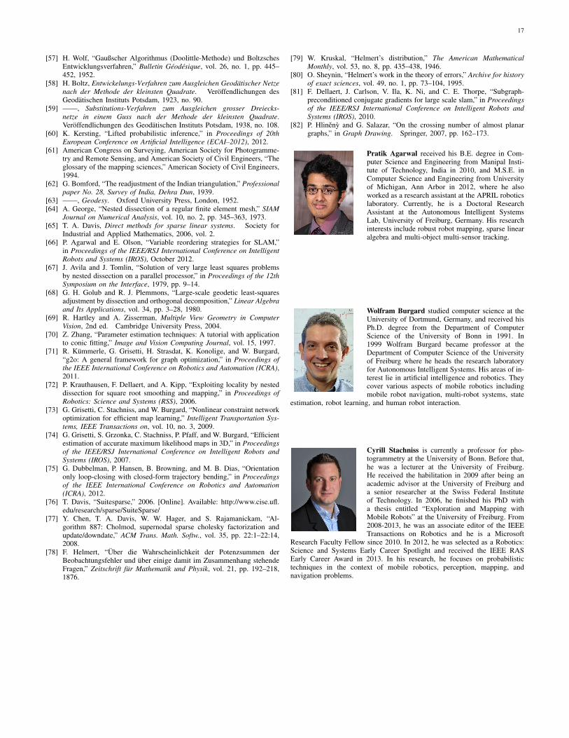
17

[57] H. Wolf, “Gaußscher Algorithmus (Doolittle-Methode) und BoltzschesEntwicklungsverfahren,” Bulletin Geodesique, vol. 26, no. 1, pp. 445–452, 1952.

[58] H. Boltz, Entwickelungs-Verfahren zum Ausgleichen Geodatischer Netzenach der Methode der kleinsten Quadrate. Veroffendlichungen desGeodatischen Instituts Potsdam, 1923, no. 90.

[59] ——, Substitutions-Verfahren zum Ausgleichen grosser Dreiecks-netze in einem Guss nach der Methode der kleinsten Quadrate.Veroffendlichungen des Geodatischen Instituts Potsdam, 1938, no. 108.

[60] K. Kersting, “Lifted probabilistic inference,” in Proceedings of 20thEuropean Conference on Artificial Intelligence (ECAI–2012), 2012.

[61] American Congress on Surveying, American Society for Photogramme-try and Remote Sensing, and American Society of Civil Engineers, “Theglossary of the mapping sciences,” American Society of Civil Engineers,1994.

[62] G. Bomford, “The readjustment of the Indian triangulation,” Professionalpaper No. 28, Survey of India, Dehra Dun, 1939.

[63] ——, Geodesy. Oxford University Press, London, 1952.[64] A. George, “Nested dissection of a regular finite element mesh,” SIAM

Journal on Numerical Analysis, vol. 10, no. 2, pp. 345–363, 1973.[65] T. A. Davis, Direct methods for sparse linear systems. Society for

Industrial and Applied Mathematics, 2006, vol. 2.[66] P. Agarwal and E. Olson, “Variable reordering strategies for SLAM,”

in Proceedings of the IEEE/RSJ International Conference on IntelligentRobots and Systems (IROS), October 2012.

[67] J. Avila and J. Tomlin, “Solution of very large least squares problemsby nested dissection on a parallel processor,” in Proceedings of the 12thSymposium on the Interface, 1979, pp. 9–14.

[68] G. H. Golub and R. J. Plemmons, “Large-scale geodetic least-squaresadjustment by dissection and orthogonal decomposition,” Linear Algebraand Its Applications, vol. 34, pp. 3–28, 1980.

[69] R. Hartley and A. Zisserman, Multiple View Geometry in ComputerVision, 2nd ed. Cambridge University Press, 2004.

[70] Z. Zhang, “Parameter estimation techniques: A tutorial with applicationto conic fitting,” Image and Vision Computing Journal, vol. 15, 1997.

[71] R. Kummerle, G. Grisetti, H. Strasdat, K. Konolige, and W. Burgard,“g2o: A general framework for graph optimization,” in Proceedings ofthe IEEE International Conference on Robotics and Automation (ICRA),2011.

[72] P. Krauthausen, F. Dellaert, and A. Kipp, “Exploiting locality by nesteddissection for square root smoothing and mapping,” in Proceedings ofRobotics: Science and Systems (RSS), 2006.

[73] G. Grisetti, C. Stachniss, and W. Burgard, “Nonlinear constraint networkoptimization for efficient map learning,” Intelligent Transportation Sys-tems, IEEE Transactions on, vol. 10, no. 3, 2009.

[74] G. Grisetti, S. Grzonka, C. Stachniss, P. Pfaff, and W. Burgard, “Efficientestimation of accurate maximum likelihood maps in 3D,” in Proceedingsof the IEEE/RSJ International Conference on Intelligent Robots andSystems (IROS), 2007.

[75] G. Dubbelman, P. Hansen, B. Browning, and M. B. Dias, “Orientationonly loop-closing with closed-form trajectory bending,” in Proceedingsof the IEEE International Conference on Robotics and Automation(ICRA), 2012.

[76] T. Davis, “Suitesparse,” 2006. [Online]. Available: http://www.cise.ufl.edu/research/sparse/SuiteSparse/

[77] Y. Chen, T. A. Davis, W. W. Hager, and S. Rajamanickam, “Al-gorithm 887: Cholmod, supernodal sparse cholesky factorization andupdate/downdate,” ACM Trans. Math. Softw., vol. 35, pp. 22:1–22:14,2008.

[78] F. Helmert, “Uber die Wahrscheinlichkeit der Potenzsummen derBeobachtungsfehler und uber einige damit im Zusammenhang stehendeFragen,” Zeitschrift fur Mathematik und Physik, vol. 21, pp. 192–218,1876.

[79] W. Kruskal, “Helmert’s distribution,” The American MathematicalMonthly, vol. 53, no. 8, pp. 435–438, 1946.

[80] O. Sheynin, “Helmert’s work in the theory of errors,” Archive for historyof exact sciences, vol. 49, no. 1, pp. 73–104, 1995.

[81] F. Dellaert, J. Carlson, V. Ila, K. Ni, and C. E. Thorpe, “Subgraph-preconditioned conjugate gradients for large scale slam,” in Proceedingsof the IEEE/RSJ International Conference on Intelligent Robots andSystems (IROS), 2010.

[82] P. Hlineny and G. Salazar, “On the crossing number of almost planargraphs,” in Graph Drawing. Springer, 2007, pp. 162–173.

Pratik Agarwal received his B.E. degree in Com-puter Science and Engineering from Manipal Insti-tute of Technology, India in 2010, and M.S.E. inComputer Science and Engineering from Universityof Michigan, Ann Arbor in 2012, where he alsoworked as a research assistant at the APRIL roboticslaboratory. Currently, he is a Doctoral ResearchAssistant at the Autonomous Intelligent SystemsLab, University of Freiburg, Germany. His researchinterests include robust robot mapping, sparse linearalgebra and multi-object multi-sensor tracking.

Wolfram Burgard studied computer science at theUniversity of Dortmund, Germany, and received hisPh.D. degree from the Department of ComputerScience of the University of Bonn in 1991. In1999 Wolfram Burgard became professor at theDepartment of Computer Science of the Universityof Freiburg where he heads the research laboratoryfor Autonomous Intelligent Systems. His areas of in-terest lie in artificial intelligence and robotics. Theycover various aspects of mobile robotics includingmobile robot navigation, multi-robot systems, state

estimation, robot learning, and human robot interaction.

Cyrill Stachniss is currently a professor for pho-togrammetry at the University of Bonn. Before that,he was a lecturer at the University of Freiburg.He received the habilitation in 2009 after being anacademic advisor at the University of Freiburg anda senior researcher at the Swiss Federal Instituteof Technology. In 2006, he finished his PhD witha thesis entitled “Exploration and Mapping withMobile Robots” at the University of Freiburg. From2008-2013, he was an associate editor of the IEEETransactions on Robotics and he is a Microsoft

Research Faculty Fellow since 2010. In 2012, he was selected as a Robotics:Science and Systems Early Career Spotlight and received the IEEE RASEarly Career Award in 2013. In his research, he focuses on probabilistictechniques in the context of mobile robotics, perception, mapping, andnavigation problems.