A Survey of Geometric Vision

Kun Huang Yi Ma

Electrical & Computer Engineering Department

University of Illinois at Urbana-Champaign

Abstract

In this chapter we give a brief survey on basic geometric principles associated with machine vision.

In particular, we introduce the basic theory and algorithms for the reconstruction of camera pose

and scene structure from two views or more than two views. We discuss further reconstruction

techniques from a single view, which utilize scene symmetry and nevertheless rely on the theory

of multiple views. Since our survey focuses on only the very basics, references to more advanced

studies will be provided after each topic. A few comprehensive examples of application of the

algorithms are given at the end of the chapter.

1 Introduction

Vision is one of the most powerful sensing modalities. In robotics, machine vision techniques have

been extensively used in applications such as manufacturing, visual servoing [30, 7], navigation

[26, 50, 51, 9], and robotic mapping [58]. Here a main problem is how to reconstruct both the pose

1

of the camera and the 3-D structure of the scene. The reconstruction inevitably requires a good

understanding about the geometry of image formation and 3-D reconstruction. In this chapter,

we provide a survey for the basic theory and some recent advances in the geometric aspect of the

reconstruction problem. Specifically, we introduce the theory and algorithms for reconstruction

from two views [33, 29, 40, 67, 31], multiple views [40, 37, 38, 23, 10, 12], and a single view

[25, 19, 1, 73, 74, 70, 3, 28]. Since this chapter can only provide a brief introduction to these

topics, the reader is referred to the book [40] for a more comprehensive coverage.

Without any knowledge of the environment, reconstruction of a scene requires multiple images.

This is because a single image is merely a 2-D projection of the 3-D world, for which the depth

information is lost. When multiple images are available from different known viewpoints, the 3-D

location of every point in the scene can be determined uniquely by triangulation (or stereopsis).

However, in many applications (especially those for robot vision), the viewpoints are unknown

either. Therefore, we need to recover both the scene structure and the camera poses. In computer

vision literature, this is referred to as the “structure from motion” (SFM) problem. To solve this

problem, the theory of multiple-view geometry has been developed (e.g., see [40, 37, 38, 67, 33, 23,

12, 10]). In this chapter, we introduce the basic theory of multiple-view geometry and show how

it can be used to develop algorithms for reconstruction purposes. Specifically, for the two-view

case, we introduce in Section 2 the epipolar constraint and the eight-point structure from motion

algorithm [33, 29, 40]. For the multiple-view case, we introduce in Section 3 the rank conditions

on multiple-view matrix [37, 38, 40, 27] and a multiple-view factorization algorithm [37, 40].

Since many robotic applications are performed in a man-made environment such as inside a

building and around an urban area, much of prior knowledge can be exploited for a more efficient

and accurate reconstruction. One kind of prior knowledge that can be utilized is the existence

2

of “regularity” in the man-made environment. For example, there exist many parallel lines, or-

thogonal corners, and regular shapes such as rectangles. In fact, much of the regularity can be

captured by the notion of symmetry. It can be shown that with sufficient symmetry, reconstruction

from a single image is feasible and accurate, and many algorithms have been developed (e.g., see

[3, 70, 25, 1, 73, 40, 28, 1]). Interestingly, these symmetry-based algorithms in fact rely on the

theory of multiple-view geometry [25, 70, 3]. Therefore, after the multiple-view case is studied,

we introduce in Section 4 basic geometry and reconstruction algorithms associated with imaging

and symmetry.

In the remainder of this section, we introduce in Section 1.1 basic notation and concepts asso-

ciated with image formation that help the development of the theory and algorithms. It is not our

intention to give in this chapter all the details about how the algorithms surveyed can be imple-

mented in real vision systems. While we will discuss briefly in Section 1.2 a pipeline for such a

system, we refer the reader to [40] for all the details.

1.1 Camera model and image formation

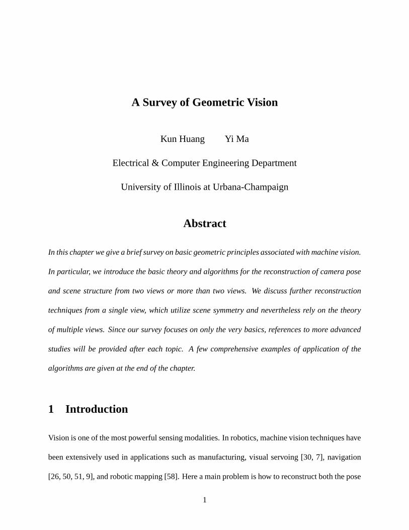
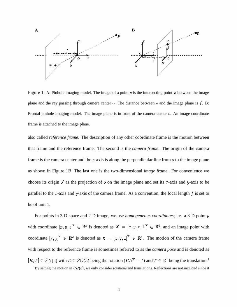
The camera model we adopt in this chapter is the commonly used pinhole camera model. As shown

in Figure 1A, the camera comprises of a camera center � and an image plane. The distance from� to the image plane is the focal length�

. For any 3-D point � in the opposite side of the image

plane with respect to � , its image � is obtained by intersecting the line connecting � and � with

the image plane. In practice, it is more convenient to use a mathematically equivalent model by

moving the image plane to the “front” side of the camera center as shown in Figure 1B.

There are usually three coordinate frames in our calculation. The first one is the world frame,

3

A B

PSfrag replacements

�� ���� ��

�� �

�� �� �� ��

Figure 1: A: Pinhole imaging model. The image of a point is the intersecting point between the image

plane and the ray passing through camera center � . The distance between � and the image plane is � . B:

Frontal pinhole imaging model. The image plane is in front of the camera center � . An image coordinate

frame is attached to the image plane.

also called reference frame. The description of any other coordinate frame is the motion between

that frame and the reference frame. The second is the camera frame. The origin of the camera

frame is the camera center and the�-axis is along the perpendicular line from � to the image plane

as shown in Figure 1B. The last one is the two-dimensional image frame. For convenience we

choose its origin � � as the projection of � on the image plane and set its � -axis and � -axis to be

parallel to the � -axis and � -axis of the camera frame. As a convention, the focal length�

is set to

be of unit 1.

For points in 3-D space and 2-D image, we use homogeneous coordinates; i.e. a 3-D point �with coordinate ������� �����������

is denoted as � �� ������� � � � �!�"�"�$#, and an image point with

coordinate ����� � � �%�'&is denoted as �(� ���)�*� � � � �%�'�

. The motion of the camera frame

with respect to the reference frame is sometimes referred to as the camera pose and is denoted as ,+ �)- �.�0/21436587with + �0/2943:5;7

being the rotation ( +<+ � �>= ) and - �?�'�being the translation.1

1By setting the motion in @BADC�EGF , we only consider rotations and translations. Reflections are not included since it

4

Therefore, for a point with coordinate � in the reference frame, its image is obtained by

H �I�% J+ �K- � � �?� � � (1)

whereH?LNM

is the depth of the 3-D point with respect to the camera center. This is the perspective

projection model of image formation.

The hat operator. One notation that will be extensively used in this chapter is the hat operator

“ O ” that denotes the skew-symmetric matrix associated to a vector in�P�

. More specifically, for a

vector QR�S ,T.U � T & � T � ���V�?� �, we define

OQXW�YZZZZZZ[

M \ T � T &T � M \ T]U\ T & T]U M^`______a

�?� �cbd� � such that OQfeV��Q>gVe � h e �?� � WIn particular, OQfQR� M �?� �

.

Similarity. We use “ i ” to denote similarity. For any pair of vectors or matrices � and j of the

same dimension, �Ii"j means �k�"lmj for some (nonzero) scalar l �n�.

1.2 3-D reconstruction pipeline

Before we delve into the geometry, we first need to know how the algorithms to be developed can

be used. Reconstruction from multiple images often consists of three steps: feature extraction,

feature matching, and reconstruction using multiple-view geometry.

Features, or image primitives, are the conspicuous image entities such as corner points, line

segments, or structures. The most commonly used image features are points and line segments.

is in ADCoEpF , but not in @BADCoEpF .5

Algorithms for extracting these features can be found in most image processing papers and hand-

books [22, 4, 18, 40]. At the end of this chapter we also give an example of using (symmetric)

structures as image features for reconstruction.

Feature matching is to establish correspondence of features across different views, which is

usually a difficult task. Many techniques have been developed to match features. For instance,

when the motion (baseline) between adjacent views is small, feature matching is often called fea-

ture tracking and typically involves finding an affine transformation between the image patches

around the feature points to be matched [34, 54]. Matching across large motion is a much more

challenging task and is still an active research area. If a large number of image points are avail-

able for matching, some statistical technique such as the RANSAC type of algorithms [13] can be

applied. Readers can refer to [23, 40] for details.

Given image features and their correspondences, the camera pose and the 3-D structure of these

features can then be recovered using the methods that will be introduced in the rest of this chapter.

1.3 Further readings

Camera calibration. In reality, there are at least two major differences between our camera model

and the real camera. First, the focal length�

of the real camera is not 1. Second, the origin of the

image coordinate frame is usually chosen at the top-left corner of the image instead of at the

center of the image. Therefore, we need to map the real image coordinate to our homogeneous

representation. This process is called camera calibration. In practice, camera calibration is more

complicated due to the pixel aspect ratio and nonlinear radial distortion of the image. The simplest

calibration scheme is to consider only the focal length and location of the image center. So the

6

actual image coordinates of a point are given by

H �q�srt J+ �K- � � � ru�YZZZZZZ[� M �wvM � �dvM M �

^`______a�?� �cbd� � (2)

where r is the calibration matrix with�

being the real focal length and �]v�����v � � being the location

of the image center in the image frame. The related theory and algorithms for camera calibration

have been studied extensively in the computer vision literature, readers can refer to [41, 71, 60, 5,

20]. In the rest of this chapter, unless otherwise stated, we assume the camera is always calibrated,

and we will use equation (1) as the camera model.

Different image surfaces. In the pinhole camera model (Figure 1) we assume that the image

plane is a planar surface. However, there are other types of image surfaces such as spheres in

omni-directional cameras. For different image surfaces, the theory that we are going to introduce

in this chapter still holds with only slight modification. Interested readers please refer to [40, 16]

for details.

Other types of projections. Besides the perspective projection model in (1), other types of pro-

jections have also been adopted in the literature for various practical or analytical purposes. For

example, there are affine projection for an uncalibrated camera, orthographic projection and weak

perspective projection for far away objects. For a detailed treatment of these projection models,

the reader please refer to [59, 11, 23].

7

2 Two-view geometry

Let us first study the two-view case. German mathematician Erwin Kruppa [32] is among the first

who studied this problem. He showed that given five pairs of corresponding points, the camera

motion and structure of the scene can be solved up to finite number of solutions [32, 24, 46]. In

practice, however, we usually can obtain more than five points, which may significantly reduce

the complexity of the solution and increase the accuracy. In 1980, Longuet-Higgins, based on

the epipolar constraint – an algebraic constraint governing two images of a point [33], developed

an efficient linear algorithm that requires eight pairs of corresponding points. The algorithm has

since been refined several times to reach the current standard eight-point linear algorithm [29, 40].

Several variations to this algorithm for coplanar point features and for continuous motions have

also been developed [67, 40]. In the remainder of this section, we introduce the epipolar constraint

and the eight-point linear algorithm.

2.1 Epipolar constraint and essential matrix

The key issue in solving two-view SFM problem is to identify the algebraic relationship between

corresponding image points and the camera motion. Figure 2 shows the relationship between the

two camera centers � U , � & , the 3-D point � with coordinate � �n��#, and its two images �xU and � & .

Obviously, the three points � U , � & and � form a plane, which implies that the vectors - , +<�DU and� & are coplanar. Mathematically, it is equivalent to the triple product of - , +<�yU and � & being zero,

i.e. � � & O- +<�xU2� M W (3)

8

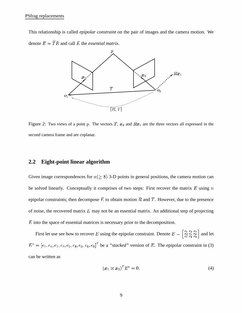
This relationship is called epipolar constraint on the pair of images and the camera motion. We

denote1 � O- + and call

1the essential matrix.

PSfrag replacements

z

{|,}�~ {D�

�f� �2� } �f�� � � �

Figure 2: Two views of a point . The vectors � , & and �P U are the three vectors all expressed in the

second camera frame and are coplanar.

2.2 Eight-point linear algorithm

Given image correspondences for � 3����873-D points in general positions, the camera motion can

be solved linearly. Conceptually it comprises of two steps: First recover the matrix1

using �epipolar constraints; then decompose

1to obtain motion + and - . However, due to the presence

of noise, the recovered matrix1

may not be an essential matrix. An additional step of projecting1into the space of essential matrices is necessary prior to the decomposition.

First let use see how to recover1

using the epipolar constraint. Denote1 ��� ��������������m��������������m��� � and let1�� �� ,��U � � # � ��� � � & � �   � � ¡ � � � � � ¢ � � £ �!� be a “stacked” version of

1. The epipolar constraint in (3)

can be written as 3 ��U�¤R� & 7 � 1 � � M � (4)

9

where ¤ denotes the Kronecker product of two vectors such that

�xU.¤N� & �S � U � & �)� U � & �K� U � & ��� U � & ��� U � & ��� U � & � � U � & � � U � & � � U � & � � �given �2¥.�¦ � ¥ �)� ¥ � � ¥ �!� ( §2� �;�©¨ ). Therefore, in the absence of noise, given � 3��s�87

pairs of image

correspondences �«ª U and ��ª & (¬­� �;�®¨¯� WGW W � � ), we can linearly solve1 �

up to a scale using the

following equation

° 1 � W�YZZZZZZZZZZ[

3 � UU ¤±� U& 7 �3 � & U ¤±� && 7 �...3 �³² U ¤±�´²& 7 �

^ __________a1 � � M � ° �?� ² b £ � (5)

and choosing1 �

as the eigenvector of° � °

associated with the eigenvalue 0.21

can then be

obtained by “unstacking”1 �

.

After obtaining1

, we can project it to the space of essential matrix and decompose it to extract

the motion, which is summarized in the following algorithm [40]:

Algorithm 1 (Eight-point structure from motion algorithm) Given � 3��>�;7pairs of image cor-

respondence of points � ª U and � ª & (¬µ� �;�®¨¯� WGW W � � ), this algorithm recovers the motion J+ �)- �of the

camera (with the first camera frame being the reference frame) in three steps.

1. Compute a first approximation of the essential matrix. Construct the matrix° �­� ² b £

as in (5). Choose1 �

to be the eigenvector of° � °

associated to its smallest eigenvalue:

compute the SVD of° �·¶´¸ / ¸B¹ �¸ and choose

1 �to be the º�»!¼ column of ¹w¸ . Unstack

1 �to obtain the

5 g 5matrix

1.

2It can be shown that for ½wC¿¾4ÀpF points in general positions, Á]¯Á has only one zero eigenvalue.

10

2. Project1

onto the space of essential matrices. Perform SVD on1

such that1 ��¶ diag ÃÅÄ�U � Ä & � Ä � Æ ¹ � �where Ä�U � Ä & � Ä � � M

and ¶ � ¹ �s/2943:5;7. The projection onto the space of essential

matrices is ¶ÈÇP¹ �with DZ� diag à �;� �;� M Æ .

3. Recover motion from by decomposing the essential matrix. The motion + and - of the

camera can be extracted from the essential matrix using ¶ and ¹ such that

+É��¶Ê+ �ËnÌÎÍÐÏ ¨³Ñ ¹ � � O- ��¶Ê+ Ë ÌÎÍ4Ï ¨³Ñ Çy¶ � �where + Ë 3 l 7 means rotation around

�-axis by l counterclockwise.

The mathematical derivation and justification for the above projection and decomposition steps can

be found in [40].

The above eight-point algorithm in general gives rise to four solutions of motion ,+ �)- �. How-

ever, only one of them guarantees that the depths of all the 3-D points reconstructed are positive

with respect to both camera frames [40]. Therefore, by checking the depths of all the points, the

unique physically possible solution can be obtained. Also notice that - is recovered up to a scale.

Without any additional scene knowledge, this scale cannot be determined and is often fixed by

setting Ò - Òp� � .Given the motion ,+ �)- �

, the next thing is to recover the structure. For point features, that

means to recover its depth with respect to the camera frame. For the ¬ th point with depthH ª ¥ in the§ th ( §«� �;�®¨ ) camera frame, from the fact

H ª & �mª & � H ª U +<��ª U]Ó - , we have

Ô ªyÕH ª W� ��Ö � & ª +<� ª U Ö� & ª - � YZZ[ H ª U�^`__a � M W (6)

11

SoH ª U can be solved by finding the eigenvector of

Ô ª � Ô ª associated to its smallest eigenvalue.

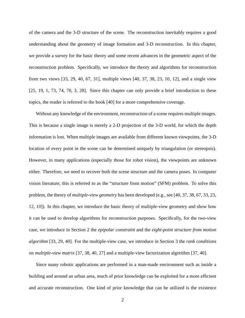
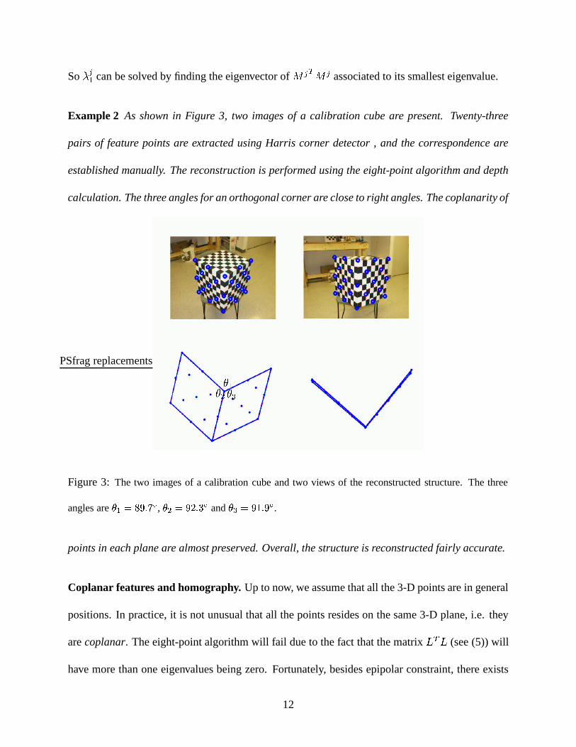
Example 2 As shown in Figure 3, two images of a calibration cube are present. Twenty-three

pairs of feature points are extracted using Harris corner detector , and the correspondence are

established manually. The reconstruction is performed using the eight-point algorithm and depth

calculation. The three angles for an orthogonal corner are close to right angles. The coplanarity of

PSfrag replacements × U× & × �

Figure 3: The two images of a calibration cube and two views of the reconstructed structure. The three

angles are Ø U«ÙqÚ�ÛdÜÞÝ ß , Ø & ÙqÛ�àdÜJá�ß and Ø � ÙâÛ;ã ÜJÛ�ß .points in each plane are almost preserved. Overall, the structure is reconstructed fairly accurate.

Coplanar features and homography. Up to now, we assume that all the 3-D points are in general

positions. In practice, it is not unusual that all the points resides on the same 3-D plane, i.e. they

are coplanar. The eight-point algorithm will fail due to the fact that the matrix° � °

(see (5)) will

have more than one eigenvalues being zero. Fortunately, besides epipolar constraint, there exists

12

another constraint for coplanar points. This is the homography between the two images, which can

be described using a matrix ä �?� �cbd�:

äå�"+ Ó �æ -èç �(7)

withækL¦M

denoting the distance from the plane to the first camera center and ç being the unit

normal vector of the plane expressed in the first camera frame withH U ç � �fU Ó æ � M

.3 It can be

shown that the two images �PU and � & of the same point are related by:

Ö� & äV��U$� M W (8)

Using the homography relationship, we can recover the motion from two views with a similar

procedure to the epipolar constraints: First ä can also be calculated linearly using � 3é�¦êë7pairs

of corresponding image points. The reason that the minimum number of point correspondences

is four instead of eight is that each pair of image points provide two independent equations onä through (8). Then the motion ,+ �)- �as well as the plane normal vector ç can be obtained by

decomposing ä . However, the solution for the decomposition is more complicated. This algorithm

is called four-point algorithm for coplanar features. Interested readers please refer to [67, 40].

2.3 Further Readings

The eight-point algorithm introduced in this section is for general situations. In practice, however,

there are several caveats:3The homography is not limited to two image points in two camera frames, it is for the coordinates of the 3-D

point on the plane expressed in any two frames (with one frame being the reference frame). In particular, if the second

frame is chosen with its origin lying on the plane, then we have a homography between the camera and the plane.

13

Small baseline motion and continuous motion. If Ò - Ò is small and data is noisy, the recon-

struction algorithm often would fail. This is the small baseline case. Readers can refer to [40, 65]

for special algorithm dealing with this situation. When the baseline become infinitesimally small,

we have the case of continuous motion, for which the algebra becomes somewhat different from

the discrete case. For a detailed analysis and algorithm, please refer to [39, 40].

Multiple-body motions. For the case in which there are multiple moving objects in the scene,

there exists a more complicated multiple-body epipolar constraint. The reconstruction algorithm

can be found in [66, 40].

Uncalibrated camera. If the camera is uncalibrated, the essential matrix1

in the epipolar con-

straint should be substituted by the fundamental matrix ì with ì��"rqí � 1 rîí U , where r �?���pbd�is the calibration matrix of the camera, defined in equation (2). The analysis and affine reconstruc-

tion for the uncalibrated camera can be found in [23, 40].

Critical surface. There are certain degenerate positions of the points for which the reconstruction

algorithm would fail. These configurations are called critical surfaces for the points. Detailed

analysis are available in [44, 40].

Numerical problems and optimization. To obtain accurate reconstruction, some numerical issues

such data normalization need to be addressed before applying the algorithm. These are discussed

in [40]. Notice that the eight-point algorithm is only a sub-optimal algorithm; various nonlinear

“optimal” algorithms have been designed, which can be found in [64, 40].

14

3 Multiple-view geometry

In this section, we study the case for reconstruction from more than two views. Specifically, we

present a set of rank conditions on a multiple-view matrix [37, 38, 27]. The epipolar constraint

for two views is just a special case implied by the rank condition. As we will see, the multiple-

view matrix associated to a geometric entity (point, line or plane) is exactly the 3-D information

that is missing in a single 2-D image but encoded in multiple ones. This approach is compact in

representation, intuitive in geometry, and simple in computation. Moreover, it provides a unified

framework for describing multiple views of all types of features and incidence relations in 3-D

space [40].

3.1 Rank condition on multiple views of point feature

PSfrag replacements

�xU � & �³ï� U � & � ï

�

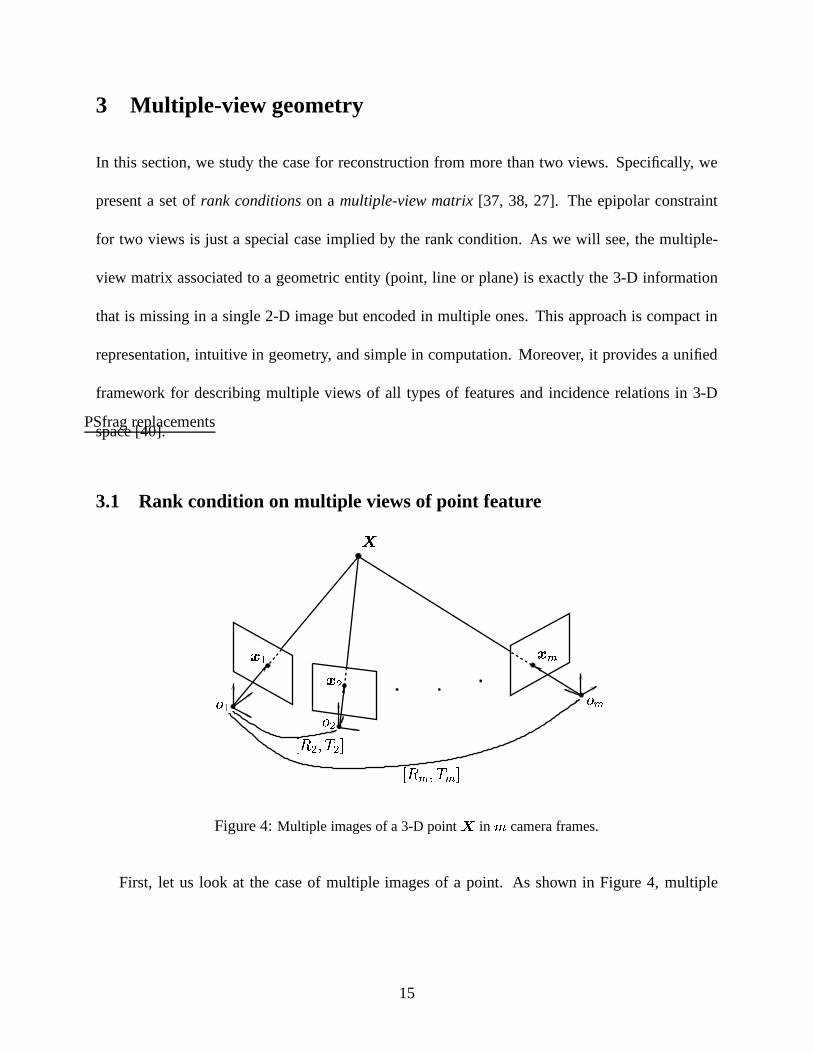
J+ & �K- & � J+èï �)- ï �Figure 4: Multiple images of a 3-D point ð in ñ camera frames.

First, let us look at the case of multiple images of a point. As shown in Figure 4, multiple

15

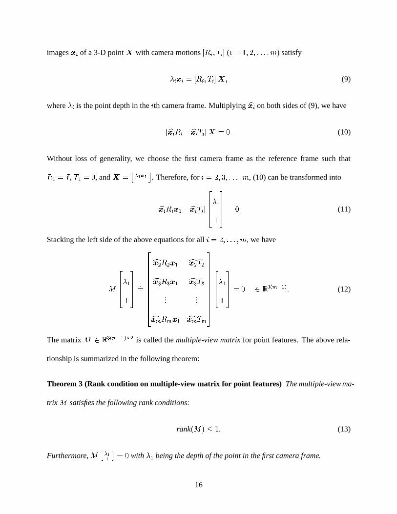
images �2¥ of a 3-D point � with camera motions J+Ê¥ �)- ¥ � ( §«� �d�®¨¯� W WGW ��ò ) satisfy

H ¥ó�´¥��S ,+è¥ �)- ¥ � � � (9)

whereH ¥ is the point depth in the § th camera frame. Multiplying O�³¥ on both sides of (9), we have

O�³¥ó+y¥ O�´¥ - ¥ � � � M W (10)

Without loss of generality, we choose the first camera frame as the reference frame such that+ôU2�s= , - U2� M, and � �uõ®ö �6÷;�USø . Therefore, for §«� ¨¯� 5 � W W W ��ò , (10) can be transformed into

O�´¥ù+西��U O�´¥ - ¥ �YZZ[ H U�

^`__a � M W (11)

Stacking the left side of the above equations for all §«� ¨¯� W WGW ��ò , we have

Ô YZZ[ H U�^ __a W�

YZZZZZZZZZZ[Ö � & + & ��U Ö� & - &Ö � � + � ��U Ö� � - �

......Ö�³ïx+yïx��U Ö�2ï - ï

^`__________aYZZ[ H U�

^ __a � M �?� �©ú ï í U:û W (12)

The matrixÔ �k����ú ï í U�û bd& is called the multiple-view matrix for point features. The above rela-

tionship is summarized in the following theorem:

Theorem 3 (Rank condition on multiple-view matrix for point features) The multiple-view ma-

trixÔ

satisfies the following rank conditions:

rank3 Ô 7xü � W (13)

Furthermore,Ô õcö �U ø � M

withH U being the depth of the point in the first camera frame.

16

The detailed proof of the theorem can be found in [37, 40].

The implication of the above theorem is multi-fold. First, the rank ofÔ

can be used to detect

the configuration of the cameras and the 3-D point. If rank3 Ô 7 � � , the cameras and the 3-D

point are in the general positions; and the location of the point can be determined (up to a scale)

by triangulation. If rank3 Ô 7 � M

, then all the camera centers and the point are collinear; and the

point can only be determined up to a line. Second, all the algebraic constraints implied by the rank

condition involve no more than three views, which means that for point features a fourth image no

longer imposes any new algebraic constraint. Last but not the least, the rank condition onÔ

uses

all the data simultaneously, which significantly simplifies the calculation. Also note that the rank

condition on the multiple-view matrix implies the epipolar constraint. For the § th ( § L � ) view and

the first view, the fact that O�³¥¿+è¥ó�fU and O�´¥ - ¥ are linearly dependent is equivalent to the epipolar

constraint between the two views.

3.2 Linear reconstruction algorithm

Now we demonstrate how to apply the multiple-view rank condition in reconstruction. Specifically,

we show the linear reconstruction algorithm for point features. Given ò 3��%5;7images of � 3��ý�87

points in 3-D space with �mª ¥ ( §Ê� �;�®¨¯� W W W ��ò and ¬0� �;�©¨¯� W W W � � ), the structure (depthsH U¥ with

respect to the first camera frame) and the camera motions ,+<¥ �)- ¥ � can be recovered in two major

steps.

17

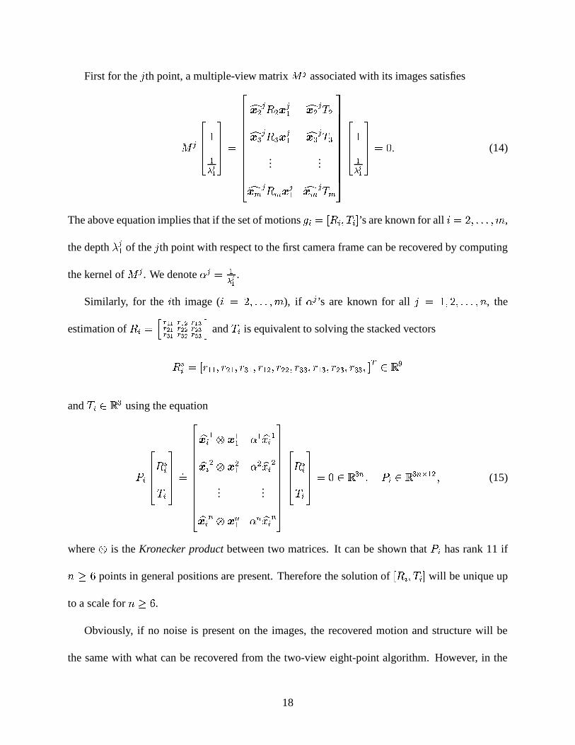
First for the ¬ th point, a multiple-view matrixÔ ª associated with its images satisfies

Ô ªYZZ[ � Uö�þ �

^`__a �YZZZZZZZZZZ[Ö � & ª + & � ª U Ö� & ª - &Ö � � ª + � ��ª U Ö� � ª - �

......Ö�³ï ª +èïf� ª U Ö�´ï ª - ï

^`__________aYZZ[ � UöKþ �

^`__a � M W (14)

The above equation implies that if the set of motions ÿ;¥*�% ,+è¥ �)- ¥ � ’s are known for all §«� ¨¯� W W W ��ò ,

the depthH ª U of the ¬ th point with respect to the first camera frame can be recovered by computing

the kernel ofÔ ª . We denote l ª � Uö þ � .

Similarly, for the § th image ( § � ¨¯� WGW W ��ò ), if l ª ’s are known for all ¬"� �;�®¨ � W W W � � , the

estimation of +è¥]� � � �ó� � �o� � ���� �:� � �ó� � �ù�� ��� � �¿� � �ó� � and - ¥ is equivalent to solving the stacked vectors

+ �¥ �% � U U ��� & U ��� � U ��� U & ��� & & ��� � � ��� U � ��� & � ��� � � � � � �n� £and - ¥ �?�'�

using the equation

� ¥YZZ[ +

�¥- ¥^`__a W�

YZZZZZZZZZZ[O�´¥ U ¤±� UU l U O� ¥ UO�´¥ & ¤±� & U l & O� ¥ &

......O�2¥ ² ¤±�´² U lm²�O� ¥ ²

^`__________aYZZ[ +

�¥- ¥^`__a � M �?� � ² � � ¥ �?� � ² b U & � (15)

where ¤ is the Kronecker product between two matrices. It can be shown that� ¥ has rank 11 if� ���

points in general positions are present. Therefore the solution of ,+<¥ �)- ¥ � will be unique up

to a scale for � ���.

Obviously, if no noise is present on the images, the recovered motion and structure will be

the same with what can be recovered from the two-view eight-point algorithm. However, in the

18

presence of noise, it is desired to use the data from all the images. In order to use the data simul-

taneously, a reasonable approach is to iterate between reconstructions of motion and structure, i.e.

initializing the structure or motions, then alternating between (14) and (15) until the structure and

motion converge.

Motions J+è¥ �K- ¥ � can then be estimated up to a scale by performing SVD on� ¥ as in (15).4

Denote+è¥ and

- ¥ to be the estimates from the eigenvector of� �¥ � ¥ associated to the smallest

eigenvalue. Let+è¥��ɶ«¥ / ¥¿¹ �¥ be the SVD of

+è¥ . Then +Ê¥ �0/29 3:587and - ¥ are given by

+�� sign3det

3 ¶«¥¿¹ �¥ 7)7 ¶m¥6¹ �¥ �0/2943:5;7 � and - ¥�� sign3det

3 ¶m¥¿¹ �¥ 7K73det

3�/ ¥ 7K7 ���?� � W (16)

In this algorithm, the initialization can be done using the eight-point algorithm for two views.

The initial estimate on the motion of second frame ,+ & �)- & � can be obtained using the standard

two-view eight-point algorithm. Initial estimates of the point depth is then

l ª � \ 3 Ö� & ª - & 7 � Ö � & ª + & �mª UÒ Ö � & ª - & Ò & � ¬µ� �d� W W W � � W (17)

In the multiple-view case, the least square estimates of point depths l ª � Uö þ � , ¬ � �;� W W W � � can be

obtained from (14) as

l ª � \� ï¥ � & 3 O�³¥!ª - ¥ 7 � O�³¥ ªp+è¥ù� ª U ï¥ � & Ò O�´¥ ª - ¥$Ò & � ¬�� �;� W W W � � W (18)

By iterating between the motion estimation and structure estimation, we expect that the esti-

mates on structure and motion converge. The convergence criteria may vary for different situa-

tions. In practice we choose the reprojected images error as the convergence criteria. For the ¬ th

3-D point, the estimate of its 3-D location can be obtained asH ª U ��ª U and the reprojection on the § th

4Now we assume that the cameras are all calibrated, which is the case of Euclidean reconstruction. This algorithm

also works for uncalibrated case.

19

image is obtained�³¥ ª i H ª U +è¥ó� ª U Ó - ¥ . Its reprojection error is then ï¥ � & Ò � ª ¥ \ �³¥ ª Ò & . So the

algorithm keep iterating until the summation of reprojection errors over all points are below some

threshold � .The algorithm is summarized below:

Algorithm 4 (A factorization algorithm for multiple-view reconstruction) Given ò 3��·587im-

ages � ª U � � ª & � W W W � � ª ï , ¬ � �;�®¨ � W W W � � of � 3é���87points, the motions ,+Ê¥ �)- ¥ � , §f� ¨¯� W WGW ��ò and the

structure of the points with respect to the first camera frame l ª , ¬4� �;�®¨¯� WGW W � � can be recovered

as follows:

1. Set the counter �� M. Compute ,+ & �K- & � using the eight-point algorithm, then get an initial

estimate of l ª from (17) for each ¬�� �;�®¨ � W W W � � . Normalize l ª�� l ª�� l U for ¬µ� �;�®¨¯� W W W � � .

2. Compute � +è¥ � - ¥ � from the eigenvector of� �¥ � ¥ corresponding its smallest eigenvalue for§«� ¨ � W W W ��ò .

3. Compute ,+Ê¥ �K- ¥ � from (16) for §³� ¨¯� 5 � W W W ��ò .

4. Compute l ª ��� U using (18) for each ¬N� �;�®¨¯� W W W � � . Normalize so that l ª�� l ª�� l U and- ¥ � l U��� U - ¥ . Use the newly recovered l ª ’s and motion ,+Ê¥ �K- ¥ � ’s to computer the reprojected

image� for each point in all views.

5. If the reprojection error Òf� \ �sÒ & L � for some threshold � L±M, then � � � Ó � and go

to step 2, otherwise stop.

The above algorithm is a direct derivation from the rank condition. There are techniques to improve

its numerical stability and statistical robustness for specific situations [40].

20

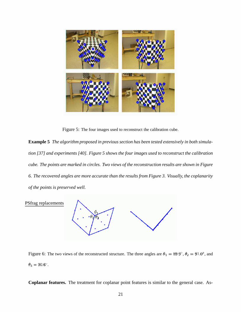
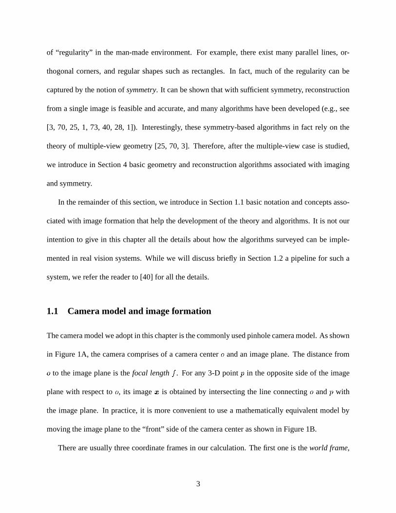
Figure 5: The four images used to reconstruct the calibration cube.

Example 5 The algorithm proposed in previous section has been tested extensively in both simula-

tion [37] and experiments [40]. Figure 5 shows the four images used to reconstruct the calibration

cube. The points are marked in circles. Two views of the reconstruction results are shown in Figure

6. The recovered angles are more accurate than the results from Figure 3. Visually, the coplanarity

of the points is preserved well.

PSfrag replacements � �� � � �

Figure 6: The two views of the reconstructed structure. The three angles are Ø U$Ù±Ú�ÛdÜJÛ ß , Ø & Ù±Û;ã Ü�� ß , andØ � ÙâÛ��;Ü���ß .Coplanar features. The treatment for coplanar point features is similar to the general case. As-

21

sume the equation of the plane in the first camera frame is õ Ï � U � Ï & ø � � Mwith Ï U ���'�

andÏ & � �. Simply appending the � g ¨ block õ Ï � U ��U � Ï & ø to the end of

Ôin (12), then the

rank condition in Theorem 3 still holds. Since Ï U � ç is the unit normal vector of the plane

and Ï & � æis the distance from the first camera center to the plane, the rank condition impliesæ 3 O�³¥ù+西�fU 7 \ 3 ç � ��U 7p3 O�³¥ - ¥ 7 � M

, which is obviously equivalent to the homography between the§ th and the first views (see (8)). As for reconstruction, we can use the four-point algorithm to

initialize the estimation of the homography and then perform similar iteration scheme to obtain

motion and structure. The algorithm can be found in [36, 51].

3.3 Further readings

Multilinear constraints and factorization algorithm. There are two other approaches dealing

with multiple-view reconstruction. The first approach is to use the so-called multilinear constraints

on multiple images of a 3-D point or line. For small number of views, these constraints can be

described in terms of tensorial notations [52, 53, 23]. For example, the constraints for ò � 5can

be described using trifocal tensors. For large number of views ( ò � �), the tensor is difficult to

describe. The reconstruction is then to calculate the trifocal tensors first and factorize the tensors

for camera motions [2]. An apparent disadvantage is that it is hard to choose the right “three-view

sets” and also difficult to combine the results. Another approach is to apply some factorization

scheme to iteratively estimate the structure and motion [57, 23, 40]. The problem for this approach

is that it is hard to initialize.

Universal multiple-view matrix and rank conditions. The reconstruction algorithm in this sec-

tion was only for point features. Algorithms have also been designed for lines features [56, 35].

22

In fact the multiple-view rank condition approach can be extended to all different types of features

such as line, plane, mixed line and point and even curves. This leads to a set of rank conditions on

a universal multiple-view matrix. For details please refer to [38, 40].

Dynamical scenes. In the constraint we developed in this section is for static scene. If the scene

is dynamic, i.e. there are moving objects in the scene, a similar type of rank condition can be

obtained. This rank condition is obtained by incorporating the dynamics of the objects in 3-D

space into its own description and lift the 3-D moving points into a higher dimensional space in

which it is static. For details please refer to [27, 40].

Orthographic projection. Finally, note that the linear algorithm and the rank condition are for

the perspective projection model. If the scene is far from the camera, then the image can be mod-

eled using orthographic projection, and the Tomasi-Kanade factorization method can be applied

[59]. Similar factorization algorithm for other types of projections and dynamics have also been

developed [48, 49, 8, 21].

4 Utilizing prior knowledge of the scene – symmetry

In this section we study how to incorporate scene knowledge into the reconstruction process. In our

daily life, especially in a man-made environment, there exist all types of “regularity.” For objects,

regular shapes such as rectangle, square, diamond, and circle always attract our attention. For

spatial relationship between objects, orthogonality, parallelism, and similarity are the conspicuous

ones. Interestingly, all the above regularities can be described using the notion of symmetry. For

instance, a rectangular window has one rotational symmetry and two reflective symmetry; the same

windows on the same wall have translational symmetry; the corner of a cube displays rotational

23

symmetry.

4.1 Symmetric multiple-view rank condition

There are many studies using instances of symmetry in the scene for reconstruction purposes [25,

19, 1, 6, 73, 74, 70, 3, 28]. Recently, a set of algorithms using symmetry for reconstruction from

a single image have been developed [25]. The main idea is to use the so-called equivalent images

encoded in a single image of a symmetric object. Figure 7 illustrates this notion for the case of a

reflective symmetry. We attach an object coordinate frame to the symmetric object and set it as

the reference frame. 3-D points � and � � are related by some symmetric transformation ÿ (in the

object frame) with ÿ 3 � 7 �s� � . In the image obtained from viewpoint9

, then the image of � � can

be interpreted as the image of � viewed from the virtual viewpoint9 � that is the correspondence

of9

under the same symmetry transformation ÿ . The image of � � is an called an equivalent

image of � viewed from9 � . Therefore, given a single image of a symmetric object, we have

multiple equivalent images of this object. The number of all equivalent images is the number of all

symmetry of the object.

In modern mathematics, symmetry of an object are characterized by a symmetry group with

each element in the group representing a transformation under which the object is invariant [68,

25]. For example, a rectangle possesses two reflective symmetry and one rotational symmetry. We

can use the group theoretic notation to define 3-D symmetric object as in [25].

Definition 6 Let/

be a set of 3-D points. It is called a symmetric structure if there exists an non-

trivial subgroup ! of the Euclidean group1 3:587

acting on/

such that for any ÿ � ! , ÿ defines an

isomorphism from/

to itself. ! is called the symmetry group of/

.

24

PSfrag replacements

"$#"%#

"

"'&)(*"%#�"'",+ �#- - &

. . &

/

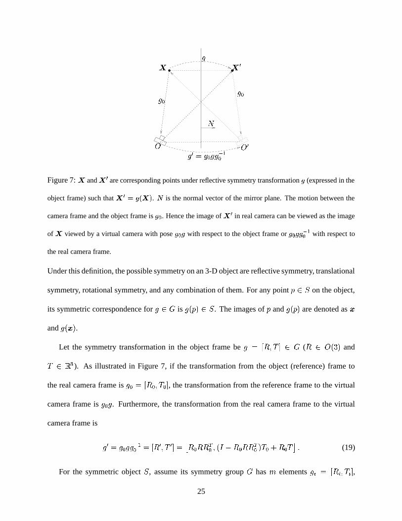
Figure 7: ð and ð � are corresponding points under reflective symmetry transformation 0 (expressed in the

object frame) such that ð � Ù 021ùð43 . 5 is the normal vector of the mirror plane. The motion between the

camera frame and the object frame is 0 v . Hence the image of ð � in real camera can be viewed as the image

of ð viewed by a virtual camera with pose 0 v 0 with respect to the object frame or 0 v 060 í Uv with respect to

the real camera frame.

Under this definition, the possible symmetry on an 3-D object are reflective symmetry, translational

symmetry, rotational symmetry, and any combination of them. For any point � �k/on the object,

its symmetric correspondence for ÿ � ! is ÿ 3 � 7y�â/. The images of � and ÿ 3 � 7 are denoted as �

and ÿ 3 � 7 .Let the symmetry transformation in the object frame be ÿs� J+ �)- � � ! ( + �t943:5;7

and- �����). As illustrated in Figure 7, if the transformation from the object (reference) frame to

the real camera frame is ÿ v � J+ v��K-�v � , the transformation from the reference frame to the virtual

camera frame is ÿ v ÿ . Furthermore, the transformation from the real camera frame to the virtual

camera frame is

ÿ � �>ÿ v ÿëÿ í Uv �% ,+ � �)- � � �uõ!+ v +<+ �v � 3 = \ + v +<+ �v 7 -�v Ó + vK- ø W (19)

For the symmetric object/

, assume its symmetry group ! has ò elements ÿ8¥ � J+è¥ �)- ¥ � ,25

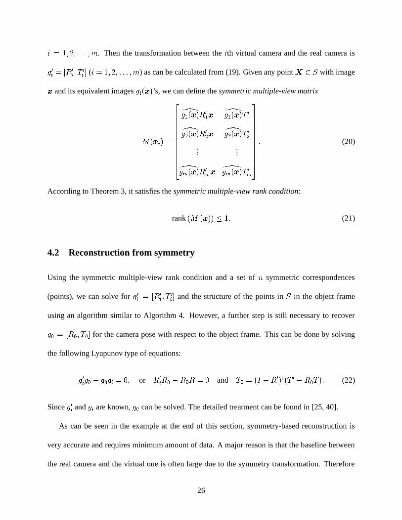
§ô� �d�®¨¯� W WGW ��ò . Then the transformation between the § th virtual camera and the real camera isÿ �¥ �ý J+ �¥ �)- �¥ � ( §«� �;�®¨¯� WGW W ��ò ) as can be calculated from (19). Given any point � �0/with image� and its equivalent images ÿ�¥ 3 � 7

’s, we can define the symmetric multiple-view matrix

Ô 3 �2¥ 7 �YZZZZZZZZZZ[

7ÿ U 3 � 7 + � U � 7ÿ U 3 � 7 -D�U7ÿ & 3 � 7 + �& � 7ÿ & 3 � 7 -D�&...

...8ÿÎï 3 � 7 + �ï � 8ÿÎï 3 � 7 -D�ï

^ __________a W (20)

According to Theorem 3, it satisfies the symmetric multiple-view rank condition:

rank3 Ô 3 � 7K7Pü � W (21)

4.2 Reconstruction from symmetry

Using the symmetric multiple-view rank condition and a set of � symmetric correspondences

(points), we can solve for ÿ �¥ � J+ �¥ �)-D�¥ � and the structure of the points in/

in the object frame

using an algorithm similar to Algorithm 4. However, a further step is still necessary to recoverÿ v � J+ v �)-*v � for the camera pose with respect to the object frame. This can be done by solving

the following Lyapunov type of equations:

ÿ �¥ ÿ v \ ÿ v ÿÎ¥*� M � or + �¥ + v \ + v +É� Mand -�v � 3 = \ + � 7:9®3 - � \ + v�- 7 W (22)

Since ÿ �¥ and ÿÎ¥ are known, ÿ v can be solved. The detailed treatment can be found in [25, 40].

As can be seen in the example at the end of this section, symmetry-based reconstruction is

very accurate and requires minimum amount of data. A major reason is that the baseline between

the real camera and the virtual one is often large due to the symmetry transformation. Therefore

26

degenerate cases will occur if the camera center is invariant under the symmetry transformation.

For example, if the camera lies on the mirror plane for a reflective symmetry, the structure can only

be recovered up to some ambiguities [25].

The reconstruction for some special cases can be simplified without explicitly using the sym-

metric multiple-view rank condition (e.g., see [3]). For the reflective symmetry, the structure with

respect to the camera frame can be calculated using only two pairs of symmetric points. Assume

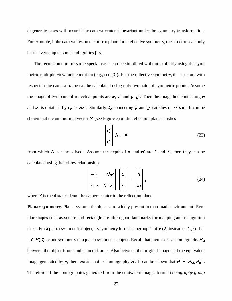
the image of two pairs of reflective points are � , � � and j , j � . Then the image line connecting �and � � is obtained by ;=<4i O�2� � . Similarly, ;=> connecting j and j � satisfies ;?> i Oj³j � . It can be

shown that the unit normal vector ç (see Figure 7) of the reflection plane satisfiesYZZ[ ;� <; � >

^`__a ç � M � (23)

from which ç can be solved. Assume the depth of � and � � areH

andH � , then they can be

calculated using the follow relationshipYZZ[ Oç � \ Oç � �ç � � ç � � �^`__a

YZZ[ HH �^`__a �

YZZ[ M¨ æ^`__a � (24)

whereæ

is the distance from the camera center to the reflection plane.

Planar symmetry. Planar symmetric objects are widely present in man-made environment. Reg-

ular shapes such as square and rectangle are often good landmarks for mapping and recognition

tasks. For a planar symmetric object, its symmetry form a subgroup ! of143 ¨ 7 instead of

143:5;7. Letÿ �V143 ¨ 7 be one symmetry of a planar symmetric object. Recall that there exists a homography ä v

between the object frame and camera frame. Also between the original image and the equivalent

image generated by ÿ , there exists another homography ä . It can be shown that ä �tä v ÿ ä í Uv .

Therefore all the homographies generated from the equivalent images form a homography group

27

ä v !ôä í Uv , which is conjugate to ! [3]. This fact can be used in testing if an image is the image

of an object with desired symmetry. Given the image, by calculating the homographies from all

equivalent images based on the hypothesis, we can check the group relationship of the homography

group and decide if the desired symmetry exists [3]. In case the object is a rectangle, the calcu-

lation can be further simplified using the notion of vanishing point as illustrated in the following

example.

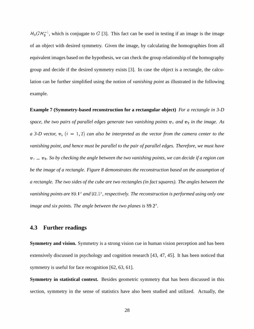
Example 7 (Symmetry-based reconstruction for a rectangular object) For a rectangle in 3-D

space, the two pairs of parallel edges generate two vanishing points e'U and e & in the image. As

a 3-D vector, e.¥ 3 §�� �d�®¨ 7 can also be interpreted as the vector from the camera center to the

vanishing point, and hence must be parallel to the pair of parallel edges. Therefore, we must havee³UA@"e & . So by checking the angle between the two vanishing points, we can decide if a region can

be the image of a rectangle. Figure 8 demonstrates the reconstruction based on the assumption of

a rectangle. The two sides of the cube are two rectangles (in fact squares). The angles between the

vanishing points are� º W � ß and º ¨ W � ß , respectively. The reconstruction is performed using only one

image and six points. The angle between the two planes is� º W ¨ ß .

4.3 Further readings

Symmetry and vision. Symmetry is a strong vision cue in human vision perception and has been

extensively discussed in psychology and cognition research [43, 47, 45]. It has been noticed that

symmetry is useful for face recognition [62, 63, 61].

Symmetry in statistical context. Besides geometric symmetry that has been discussed in this

section, symmetry in the sense of statistics have also been studied and utilized. Actually, the

28

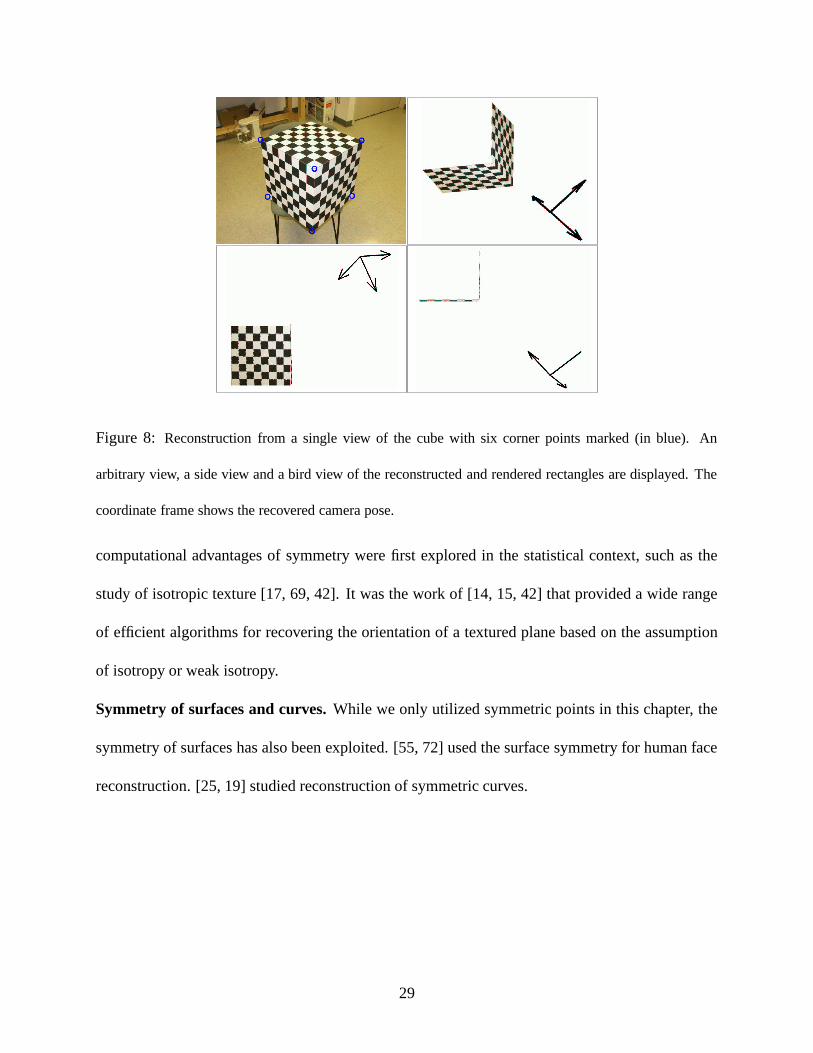
Figure 8: Reconstruction from a single view of the cube with six corner points marked (in blue). An

arbitrary view, a side view and a bird view of the reconstructed and rendered rectangles are displayed. The

coordinate frame shows the recovered camera pose.

computational advantages of symmetry were first explored in the statistical context, such as the

study of isotropic texture [17, 69, 42]. It was the work of [14, 15, 42] that provided a wide range

of efficient algorithms for recovering the orientation of a textured plane based on the assumption

of isotropy or weak isotropy.

Symmetry of surfaces and curves. While we only utilized symmetric points in this chapter, the

symmetry of surfaces has also been exploited. [55, 72] used the surface symmetry for human face

reconstruction. [25, 19] studied reconstruction of symmetric curves.

29

5 Comprehensive examples and experiments

Finally, we discuss several applications of using the techniques introduced in this chapter. These

applications all involve reconstruction from a single or multiple images for the purpose of robotic

navigation and mapping. While not all of them are fully automatic, they demonstrate the potential

of the techniques discussed in this chapter and some future directions for improvement.

5.1 Automatic landing of unmanned aerial vehicles

Figure 9: Top: A picture of the UAV in landing process. Bottom Left: An image of the landing pad viewed

from an on-board camera. Bottom Right: Extracted corner features from the image of the landing pad.

(Photo courtesy of O. Shankeria)

Figure 9 displays the experiment setup for applying the multiple-view rank condition based

algorithm in automatic landing of UAV in University of California at Berkeley [51]. In this ex-

periment, the UAV is a model helicopter (Figure 9 Top) with an on-board video camera facing

30

downwards searching for the landing pad (Figure 9 Bottom left) on the ground. When the landing

pad is found, corner points are extracted from each image in the video sequence (Figure 9 Bottom

right). The pose and the motion of the camera (and the UAV) are estimated using the feature points

in the images. Previously the four-point two-view reconstruction algorithm for planar features

was tested. However, its results were noisy (Figure 10 Left). Later an nonlinear two-view algo-

rithm was developed, but it was time consuming. Finally, by adopting the rank condition based

multiple-view algorithm, the landing problem was solved.

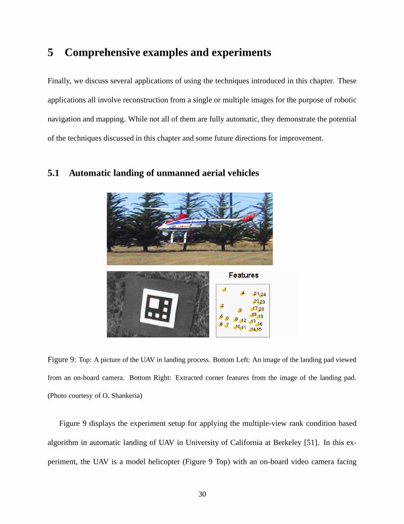
The multiple-view reconstruction are performed for every four images at 10Hz. The algorithm

is a modification of the Algorithm 4 introduced in this chapter, which is specifically designed for

coplanar features. Figure 10 shows the comparison of this algorithm with other algorithms and

sensors. The multiple-view algorithm is more accurate than both two-view algorithms (Figure 10

Left) and is close to the results obtained from differential GPS and INS sensors (Figure 10 Right).

The overall error for this algorithm is less then 5cm in distance andê ß for rotation [51].

X Y Z0

5

10

15

20

25

30

35Comparison of Motion Estimation Algorithms

Tra

nsla

tion

erro

r (c

m) linear 2−view

nonlinearmulti−view

X Y Z0

2

4

6

8

10

12

14

Rot

atio

n er

ror(

degr

ees) linear 2−view

nonlinearmulti−view

2 4 6 8 10 12 14 16 1864.2

64.4

64.6

64.8

x−po

s (m

)

2 4 6 8 10 12 14 16 18

−56.8

−56.6

−56.4

−56.2

y−po

s (m

)

2 4 6 8 10 12 14 16 18

−3.4

−3.2

−3

−2.8

time (seconds)

z−po

s (m

)

Multi−View State Estimate (red) vs INS/GPS State (blue)

Figure 10: Left: Comparison of the multiple-view rank condition based algorithm with two view linear

algorithm and nonlinear algorithm. Right: Comparison of the results from multiple-view rank condition

based algorithm (red line) with GPS and INS results (blue line). (Image courtesy of O. Shankeria.)

31

5.2 Automatic symmetry cell detection, matching and reconstruction

In Section 4, we discussed symmetry-based reconstruction techniques from a single image. Here

we present a comprehensive example that performs symmetry-based reconstruction from multiple

views [3, 28]. In this example, the image primitives are no longer point or line. Instead we use the

symmetry cells as features. The example includes three steps:

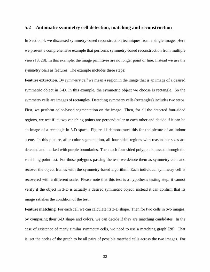
Feature extraction. By symmetry cell we mean a region in the image that is an image of a desired

symmetric object in 3-D. In this example, the symmetric object we choose is rectangle. So the

symmetry cells are images of rectangles. Detecting symmetry cells (rectangles) includes two steps.

First, we perform color-based segmentation on the image. Then, for all the detected four-sided

regions, we test if its two vanishing points are perpendicular to each other and decide if it can be

an image of a rectangle in 3-D space. Figure 11 demonstrates this for the picture of an indoor

scene. In this picture, after color segmentation, all four-sided regions with reasonable sizes are

detected and marked with purple boundaries. Then each four-sided polygon is passed through the

vanishing point test. For those polygons passing the test, we denote them as symmetry cells and

recover the object frames with the symmetry-based algorithm. Each individual symmetry cell is

recovered with a different scale. Please note that this test is a hypothesis testing step, it cannot

verify if the object in 3-D is actually a desired symmetric object, instead it can confirm that its

image satisfies the condition of the test.

Feature matching. For each cell we can calculate its 3-D shape. Then for two cells in two images,

by comparing their 3-D shape and colors, we can decide if they are matching candidates. In the

case of existence of many similar symmetry cells, we need to use a matching graph [28]. That

is, set the nodes of the graph to be all pairs of possible matched cells across the two images. For

32

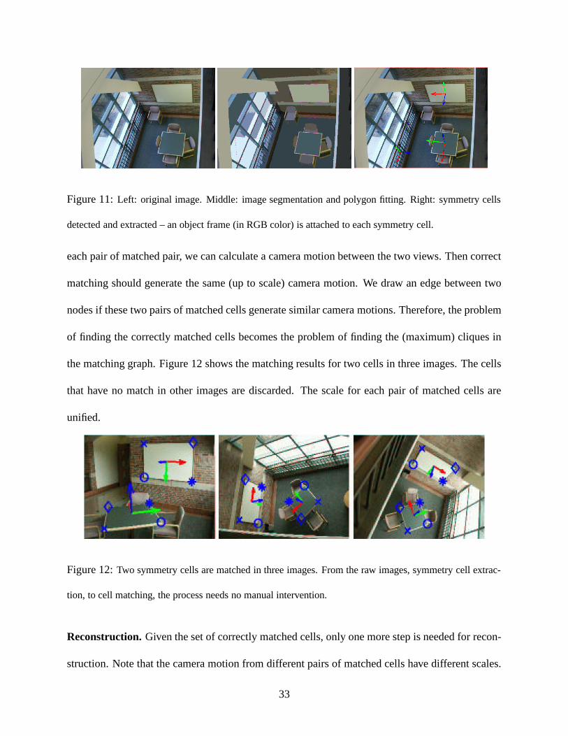
Figure 11: Left: original image. Middle: image segmentation and polygon fitting. Right: symmetry cells

detected and extracted – an object frame (in RGB color) is attached to each symmetry cell.

each pair of matched pair, we can calculate a camera motion between the two views. Then correct

matching should generate the same (up to scale) camera motion. We draw an edge between two

nodes if these two pairs of matched cells generate similar camera motions. Therefore, the problem

of finding the correctly matched cells becomes the problem of finding the (maximum) cliques in

the matching graph. Figure 12 shows the matching results for two cells in three images. The cells

that have no match in other images are discarded. The scale for each pair of matched cells are

unified.

Figure 12: Two symmetry cells are matched in three images. From the raw images, symmetry cell extrac-

tion, to cell matching, the process needs no manual intervention.

Reconstruction. Given the set of correctly matched cells, only one more step is needed for recon-

struction. Note that the camera motion from different pairs of matched cells have different scales.

33

To unify the scale, we pick one pair of matched cells as the reference to calculate the translation

and use this translation to scale the rest matched pairs. The new scales can further be passed to

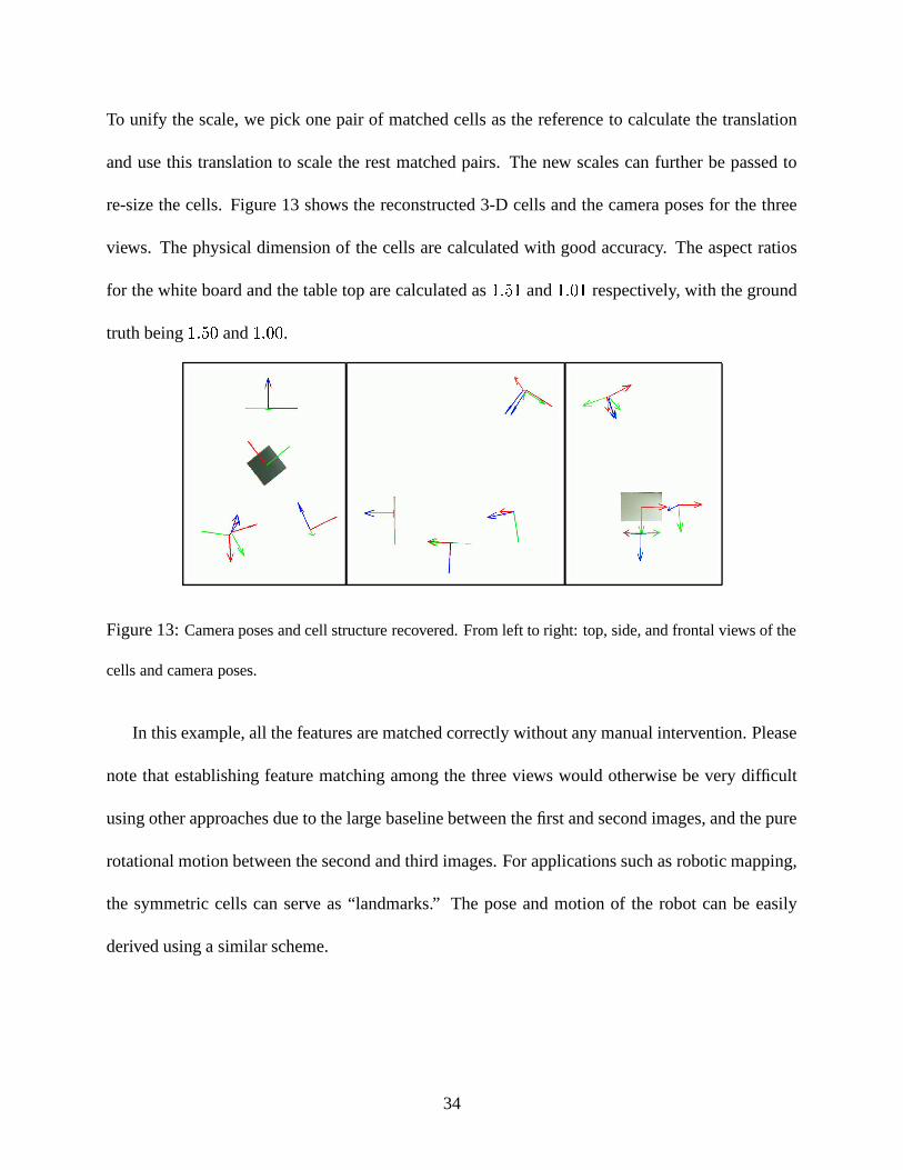
re-size the cells. Figure 13 shows the reconstructed 3-D cells and the camera poses for the three

views. The physical dimension of the cells are calculated with good accuracy. The aspect ratios

for the white board and the table top are calculated as � W � � and � W M � respectively, with the ground

truth being � W � M and � W M;M .

Figure 13: Camera poses and cell structure recovered. From left to right: top, side, and frontal views of the

cells and camera poses.

In this example, all the features are matched correctly without any manual intervention. Please

note that establishing feature matching among the three views would otherwise be very difficult

using other approaches due to the large baseline between the first and second images, and the pure

rotational motion between the second and third images. For applications such as robotic mapping,

the symmetric cells can serve as “landmarks.” The pose and motion of the robot can be easily

derived using a similar scheme.

34

5.3 Semi-automatic building mapping and reconstruction

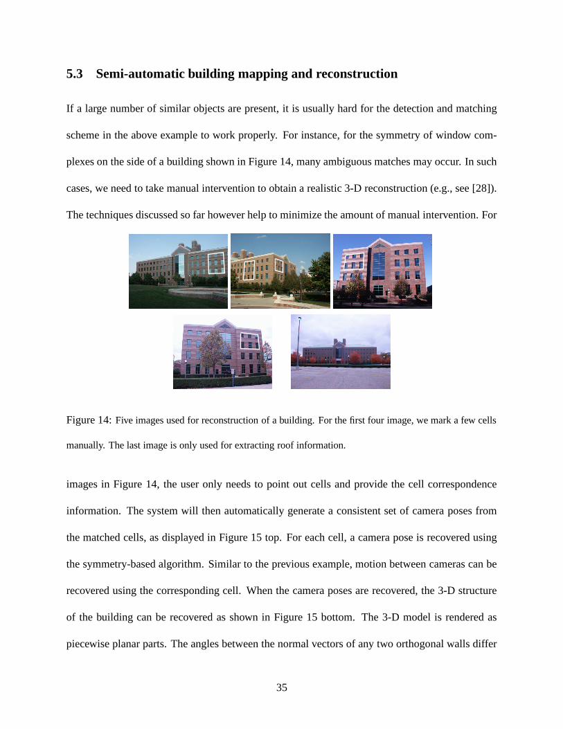
If a large number of similar objects are present, it is usually hard for the detection and matching

scheme in the above example to work properly. For instance, for the symmetry of window com-

plexes on the side of a building shown in Figure 14, many ambiguous matches may occur. In such

cases, we need to take manual intervention to obtain a realistic 3-D reconstruction (e.g., see [28]).

The techniques discussed so far however help to minimize the amount of manual intervention. For

Figure 14: Five images used for reconstruction of a building. For the first four image, we mark a few cells

manually. The last image is only used for extracting roof information.

images in Figure 14, the user only needs to point out cells and provide the cell correspondence

information. The system will then automatically generate a consistent set of camera poses from

the matched cells, as displayed in Figure 15 top. For each cell, a camera pose is recovered using

the symmetry-based algorithm. Similar to the previous example, motion between cameras can be

recovered using the corresponding cell. When the camera poses are recovered, the 3-D structure

of the building can be recovered as shown in Figure 15 bottom. The 3-D model is rendered as

piecewise planar parts. The angles between the normal vectors of any two orthogonal walls differ

35

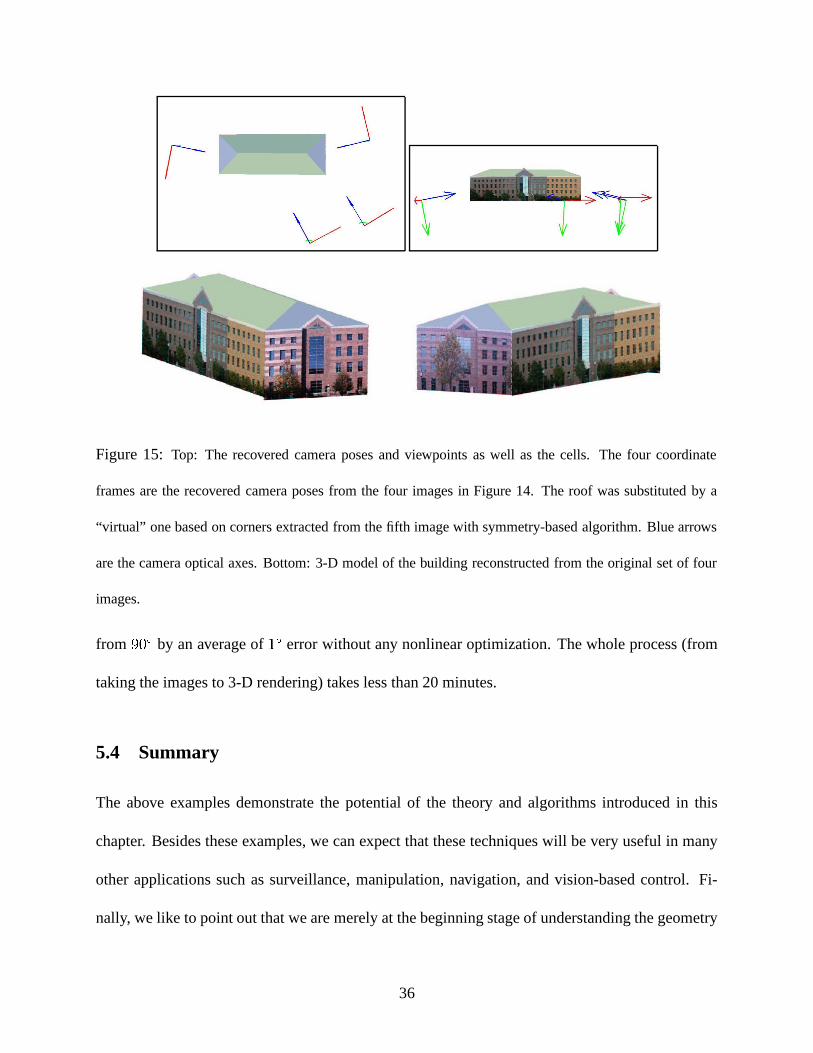
Figure 15: Top: The recovered camera poses and viewpoints as well as the cells. The four coordinate

frames are the recovered camera poses from the four images in Figure 14. The roof was substituted by a

“virtual” one based on corners extracted from the fifth image with symmetry-based algorithm. Blue arrows

are the camera optical axes. Bottom: 3-D model of the building reconstructed from the original set of four

images.

from º M ß by an average of � ß error without any nonlinear optimization. The whole process (from

taking the images to 3-D rendering) takes less than 20 minutes.

5.4 Summary

The above examples demonstrate the potential of the theory and algorithms introduced in this

chapter. Besides these examples, we can expect that these techniques will be very useful in many

other applications such as surveillance, manipulation, navigation, and vision-based control. Fi-

nally, we like to point out that we are merely at the beginning stage of understanding the geometry

36

and dynamics associated with visual perception. Much of the topological, geometric, metric, and

dynamical relations between 3-D space and 2-D images is still largely unknown, which, to some

extent, explains why the capability of existing machine vision systems are still far inferior to that

of human vision.

References

[1] A.R.J.Francois, G.G.Medioni, and R.Waupotitsch. Reconstructing mirror symmetric scenes from a

single view using 2-view stereo geometry. In Proceedings of International Conference on Pattern

Recognition, 2002.

[2] S. Avidan and A. Shashua. Novel view synthesis by cascading trilinear tensors. IEEE Transactions on

Visualization and Computer Graphics, 4(4), 1998.

[3] A.Y.Yang, S.Rao, K. Huang, W. Hong, and Y. Ma. Geometric segmentation of perspective images

based on symmetry groups. In Proceedings of IEEE International Conference on Computer Vision,

Nice, France, 2003.

[4] J. F. Canny. A computational approach to edge detection. IEEE Transactions on Pattern Analysis &

Machine Intelligence, 8(6):679–698, 1986.

[5] B. Caprile and V. Torre. Using vanishing points for camera calibration. International Journal on

Computer Vision, 4(2):127–140, 1990.

[6] S. Carlsson. Symmetry in perspective. In Proceedings of European Conference on Computer Vision,

pages 249–263, 1998.

[7] P. I. Corke. Visual Control of Robots: High-Performance Visual Servoing. Robotics and Mechatronics

Series. Research Studies Press LTD, 1996.

37

[8] J. Costeira and T. Kanade. A multi-body factorization method for motion analysis. In Proceedings of

IEEE International Conference on Computer Vision, pages 1071–1076, 1995.

[9] A.K. Das, R. Fierro, V. Kumar, B. Southball, J.Spletzer, and C.J.Taylor. Real-time vision-based control

of a nonholonomic mobile robot. In Proceedings of IEEE International Conference and Robotics and

Automation, ”2002”.

[10] O. Faugeras. There-Dimensional Computer Vision. The MIT Press, 1993.

[11] O. Faugeras. Stratification of three-dimensional vision: projective, affine, and metric representations.

Journal of the Optical Society of America, 12(3):465–84, 1995.

[12] O. Faugeras and Q.-T. Luong. Geometry of Multiple Images. The MIT Press, 2001.

[13] M. A. Fischler and R. C. Bolles. Random sample consensus: a paradigm for model fitting with ap-

plication to image analysis and automated cartography. Communications of ACM, 24(6):381–395,

1981.

[14] J. Garding. Shape from texture for smooth curved surfaces in perspective projection. Journal of

Mathematical Imaging and Vision, 2(4):327–350, 1992.

[15] J. Garding. Shape from texture and contour by weak isotropy. Journal of Artificial Intelligence,

64(2):243–297, 1993.

[16] C. Geyer and K. Daniilidis. Properties of the catadioptric fundamental matrix. In Proceedings of

European Conference on Computer Vision, Copenhagen, Denmark, 2002.

[17] J. Gibson. The Perception of the Visual World. Houghton Mifflin, 1950.

[18] R. Gonzalez and R. Woods. Digital Image Processing. Addison-Wesley, 1992.

38

[19] L. Van Gool, T. Moons, and M. Proesmans. Mirror and point symmetry under perspective skewing. In

International Conference on Computer Vision & Pattern Recognition, San Francisco, USA, 1996.

[20] A. Gruen and T. Huang. Calibration and Orientation of Cameras in Computer Vision. Information

Sciences. Springer-Verlag, 2001.

[21] M. Han and T. Kanade. Reconstruction of a scene with multiple linearly moving objects. In Interna-

tional Conference on Computer Vision & Pattern Recognition, volume 2, pages 542–549, 2000.

[22] C. Harris and M. Stephens. A combined corner and edge detector. In Proceedings of the Alvey Con-

ference, pages 189–192, 1988.

[23] R. Hartley and A. Zisserman. Multiple View Geometry in Computer Vision. Cambridge, 2000.

[24] A. Heyden and G. Sparr. Reconstruction from calibrated cameras – a new proof of the Kruppa De-

mazure theorem. Journal of Mathematical Imaging and Vision, pages 1–20, 1999.

[25] W. Hong. Geometry and reconstruction from spatial symmetry. Master Thesis, UIUC, July 2003.

[26] B. Horn. Robot Vision. MIT Press, 1986.

[27] K. Huang, R. Fossum, and Y. Ma. Generalized rank conditions in multiple view geometry with appli-

cation to dynamic. In Proceedings of the 6th European Conference on Computer Vision, Copenhagen,

Denmark, 2002.

[28] K. Huang, W. Hong, Y. Yang, and Y. Ma. Symmetry-based structure from perspecitve images, part

ii: Matching and correspondence. Submitted to IEEE Transactions on Pattern Analysis and Machine

Intellegence, 2003.

[29] T. Huang and O. Faugeras. Some properties of the E matrix in two-view motion estimation. IEEE

Transactions on Pattern Analysis & Machine Intelligence, 11(12):1310–12, 1989.

39

[30] S. Hutchinson, G. D. Hager, and P. I. Corke. A tutorial on visual servo control. IEEE Transactions on

Robotics and Automation, pages 651–670, 1996.

[31] K. Kanatani. Geometric Computation for Machine Vision. Oxford Science Publications, 1993.

[32] E. Kruppa. Zur ermittlung eines objecktes aus zwei perspektiven mit innerer orientierung. Sitz.-

Ber.Akad.Wiss., Math.Naturw., Kl.Abt.IIa, 122:1939-1948, 1913.

[33] H. C. Longuet-Higgins. A computer algorithm for reconstructing a scene from two projections. Nature,

293:133–135, 1981.

[34] B.D. Lucas and T. Kanade. An iterative image registration technique with an application to stereo

vision. In Proceedings of the Seventh International Joint Conference on Artificial Intelligence, pages

674–679, 1981.

[35] Y. Ma, K. Huang, and J. Kosecka. New rank deficiency condition for multiple view geometry of line

features. technical report, May 8, 2001.

[36] Y. Ma, K. Huang, and R. Vidal. Rank deficiency of the multiple view matrix for planar features. UIUC,

CSL Technical Report, UILU-ENG 01-2209 (DC-201), May 18, 2001.

[37] Y. Ma, K. Huang, R. Vidal, J. Kosecka, and S. Sastry. Rank conditions of multiple view matrix in

multiple view geometry. International Journal of Computer Vision, To appear.

[38] Y. Ma, J. Kosecka, and K. Huang. Rank deficiency condition of the multiple view matrix for mixed

point and line features. In Proceedings of Asian Conference on Computer Vision, Sydney, Australia,

2002.

[39] Y. Ma, J. Kosecka, and S. Sastry. Motion recovery from image sequences: Discrete viewpoint vs.

differential viewpoint. In Proceedings of European Conference on Computer Vision, Volume II, pages

337–53, 1998.

40

[40] Y. Ma, S. Soatto, J. Kosecka, and S. Sastry. An Invitation to 3D Vision: From Images to Geometric

Models. Springer-Verlag, 2003.

[41] Y. Ma, Rene Vidal, J. Kosecka, and S. Sastry. Kruppa’s equations revisited: its degeneracy, renormal-

ization and relations to cherality. In Proceedings of European Conference on Computer Vision, Dublin,

Ireland, 2000.

[42] J. Malik and R. Rosenholtz. Computing local surface orientation and shape from texture for curved

surfaces. International Journal on Computer Vision, 23:149–168, 1997.

[43] D. Marr. Vision: a computational investigation into the human representation and processing of visual

information. W.H. Freeman and Company, 1982.

[44] S. Maybank. Theory of Reconstruction from Image Motion. Springer Series in Information Sciences.

Springer-Verlag, 1993.

[45] D. Morales and H. Pashler. No role for colour in symmetry perception. Nature, 399:115–116, May

1999.

[46] D. Nister. An efficient solution to the five-point relative pose problem. In CVPR, Madison, USA, 2003.

[47] S. E. Plamer. Vision Science: Photons to Phenomenology. The MIT Press, 1999.

[48] C. J. Poelman and T. Kanade. A paraperspective factorization method for shape and motion recovery.

IEEE Transactions on Pattern Analysis and Machine Intelligence, 19(3):206–18, 1997.

[49] L. Quan and T. Kanade. A factorization method for affine structure from line correspondences. In

International Conference on Computer Vision & Pattern Recognition, pages 803–808, 1996.

[50] L. Robert, C. Zeller, O. Faugeras, and M. Hebert. Applications of nonmetric vision to some visually

guided tasks. In I. Aloimonos, editor, Visual Navigation, pages 89–135, 1996.

41

[51] O. Shakernia, R. Vidal, C. Sharp, Y. Ma, and S. Sastry. Multiple view motion estimation and control

for landing an unmanned aerial vehicle. In Proceedings of International Conference on Robotics and

Automation, 2002.

[52] A. Shashua. Trilinearity in visual recognition by alignment. In Proceedings of European Conference

on Computer Vision, pages 479–484. Springer-Verlag, 1994.

[53] A. Shashua and L. Wolf. On the structure and properties of the quadrifocal tensor. In the Proceedings

of ECCV, Volume I, pages 711–724. Springer-Verlag, 2000.

[54] J. Shi and C. Tomasi. Good features to track. In IEEE Conference on Computer Vision and Pattern

Recognition, pages 593–600, 1994.

[55] I. Shimshoni, Y. Moses, and M. Lindenbaum. Shape reconstruction of 3D bilaterally symmetric sur-

faces. International Journal on Computer Vision, 39:97–112, 2000.

[56] M. Spetsakis and Y. Aloimonos. Structure from motion using line correspondences. International

Journal of Computer Vision, 4(3):171–184, 1990.

[57] P. Sturm and B. Triggs. A factorizaton based algorithm for multi-image projective structure and mo-

tion. In Proceedings of European Conference on Computer Vision, pages 709–720. IEEE Comput.

Soc. Press, 1996.

[58] S. Thrun. Robotic mapping: A survey. CMU-CS-02-111, February 2002.

[59] C. Tomasi and T. Kanade. Shape and motion from image streams under orthography. Intl. Journal of

Computer Vision, 9(2):137–154, 1992.

[60] B. Triggs. Autocalibration from planar scenes. In Proceedings of IEEE conference on Computer Vision

and Pattern Recognition, 1998.

42

[61] N.F. Troje and H.H. Bulthoff. How is bilateral symmetry of human faces used for recognition of novel

views. Vision Research, 38(1):79–89, 1998.

[62] T. Vetter and T. Poggio. Symmetric 3d objects are an easy case for 2d object recognition. Spatial

Vision, 8:443–453, 1994.

[63] T. Vetter, T. Poggio, and H. H. Bulthoff. The importance of symmetry and virtual views in three-

dimensional object recognition. Current Biology, 4:18–23, 1994.

[64] R. Vidal, Y. Ma, S. Hsu, and S. Sastry. Optimal motion estimation from multiview normalized epipolar

constraint. In Proceedings of IEEE International Conference on Computer Vision, Vancouver, Canada,

2001.

[65] R. Vidal and J. Oliensis. Structure from planar motion with small baselines. In Proceedings of Euro-

pean Conference on Computer Vision, pages 383–398, Copenhagen, Denmark, 2002.

[66] R. Vidal, S. Soatto, Y. Ma, and S. Sastry. Segmentation of dynamic scenes from the multibody fun-

damental matrix. In Proceedings of ECCV workshop on Vision and Modeling of Dynamic Scenes,

2002.

[67] J. Weng, T. S. Huang, and N. Ahuja. Motion and Structure from Image Sequences. Springer Verlag,

1993.

[68] H. Weyl. Symmetry. Princeton Univ. Press, 1952.

[69] A. P. Witkin. Recovering surface shape and orientation from texture. Journal of Artificial Intelligence,

17:17–45, 1988.

[70] A.Y. Yang, W. Hong, and Y. Ma. Structure and pose from single images of symmetric objects with

applications in robot navigationi. In Proceedings of International Conference on Robotics and Au-

tomation, Taipei, 2003.

43

[71] Z. Zhang. A flexible new technique for camera calibration. Microsoft Technical Report MSR-TR-98-71,

1998.

[72] W. Y. Zhao and R. Chellappa. Symmetric shape-from-shading using self-ratio image. International

Journal on Computer Vision, 45(1):55–75, 2001.

[73] A. Zisserman, D. P. Mukherjee, and J. M. Brady. Shape from symmetry-detecting and exploiting

symmetry in affine images. Phil. Trans. Royal Soc. London A, 351:77–106, 1995.

[74] A. Zisserman, C. A. Rothwell, D. A. Forsyth, and J. L. Mundy. Extracting projective structure from

single perspective views of 3d point sets. In Proceedings of IEEE International Conference on Com-

puter Vision, 1993.

44