A Survey of Hyperspectral Image Classification in -

ISSN (Print) : 2319-5940 ISSN (Online) : 2278-1021

International Journal of Advanced Research in Computer and Communication Engineering

Vol. 2, Issue 8, August 2013

Copyright to IJARCCE www.ijarcce.com 2986

A Survey of Hyperspectral Image Classification

in Remote Sensing

R.Ablin1, C.Helen Sulochana

2

Assistant Professor, Electronics and Communication Engg., Arunachala College of Engineering for Women,

Affiliated to Anna University Chennai, Tamilnadu, India

Professor, Electronics and Communication Engg., St.Xavier’s Catholic College of Engineering,

Affiliated to Anna University Chennai, Tamilnadu, India

Abstract: Hyperspectral image processing has been a very dynamic area in remote sensing and other applications in

recent years. Hyperspectral images provide ample spectral information to identify and distinguish spectrally similar

materials for more accurate and detailed information extraction. Wide range of advanced classification techniques are

available based on spectral information and spatial information. To improve classification accuracy it is essential to

identify and reduce uncertainties in image processing chain. This paper presents the current practices, problems and

prospects of hyperspectral image classification. In addition, some important issues affecting classification performance

are discussed.

Keywords: Hyperspectral image classification; Per-Pixel; Subpixel; Per-field; Supervised Classification.

I. INTRODUCTION

Remote sensing can be defined as collection and

interpretation of information about an object, area or event

without any physical contact with the object. Aircraft and

satellites are the common platforms for remote sensing of

earth and its natural resources (Goetz et al., 1985). Aerial

photography in visible portion of the electromagnetic

wavelength was the original form of remote sensing but

technological developments has enabled the acquisition of

information at other wavelength including near infrared,

thermal infrared and microwave. Collection of information

over a large numbers of wavelength bands is referred as

hyperspectral data. Remote Sensing involves measurement

of energy in various parts of the electromagnetic spectrum.

A spectral band is defined as a discrete interval of the

Electromagnetic spectrum. For example the wavelengths

range is 0.4 micrometers to 0.5micrometers in one spectral

band.

In remote sensing, a detector measures the

electromagnetic radiation which is reflected from the

earth’s surface materials. These measurements help to

distinguish the type of land cover soil, water and

vegetation that has different patterns of reflectance and

absorption over different wavelengths. For example, the

reflectance of radiation from soil varies over the range of

wavelengths in the electromagnetic spectrum known as

spectral signature of the material. All earth surface

features including minerals, vegetation, dry soil, water and

snow have unique spectral reflectance signatures.

Hyperspectral imaging is concerned with analysis and

interpretation of spectra acquired from a given scene at a

short, medium or long distance by an airborne or satellite

sensor. This system is able to cover the wavelength region

from 0.4 to 2.5 micrometers using more than two hundred

spectral channels at nominal spectral resolution of 10

nanometers. Hyperspectral Signature detects the individual

absorption features of all materials, because all the

materials are bound by chemical bonds. Hence

hyperspectral data is used to detect fine changes in

vegetation, soil, water and mineral reflectance.

Hyperspectral remote sensing image analysis also attracts

a growing interest in real-world applications such as urban

planning, agriculture, forestry and monitoring.

Hyperspectral data contain extremely rich spectral

attributes, which offer the potential to discriminate more

detailed classes with classification accuracy.

Hyperspectral image classification is the process used to

produce thematic maps from remote sensing image. A

thematic map represents the earth surface objects (Soil,

vegetation, roof, road, buildings) and its construction

implies the themes or categories selected for the map are

distinguishable in image. Classification in remote sensing

involves clustering the pixels of an image to a set of

classes such that pixels in the same class are having

similar properties. One of the important problems in

remote sensing is huge amount of data that is typically

available for processing. To combat the data explosion

problem, internal and fuzzy methods were employed

(Starks. S.A & EI Paso, 2001). Majority of Image

classification is based on the detection of the spectral

response patterns of land cover classes.

In this Literature, many supervised and unsupervised

classification have been developed to tackle the

hyperspectral image Classification problem. The rest of

this paper is organized as follows. Section 2 reviews the

various hyperspectral Image Classification approaches,





section 3 describes about the dataset description and

section 4 draws the conclusion.

II. HYPERSPECTRAL IMAGE CLASSIFICATION

APPROACHES

The overall objective of image classification procedures is

to automatically categorize all pixels in image into land

cover classes (Lu & Weng, 2007). Based on pixel

information, Images can be classified as Per-pixel,

Subpixel, Per-field, Knowledge based, Contextual and

multiple classifiers. Per-pixel classifiers may be

parametric or non-parametric. Based on the use of training

samples, images can be classified as Supervised and

Unsupervised Classification. The unsupervised

classification is the identification of natural groups or

structures. The supervised classification is the process of

using samples of known identity to classify (i.e.) to assign

unclassified pixels to one of several informational classes.

Supervised method follows the steps such as feature

extraction, training and labeling processes. The first step

consists of transforming the image to a feature image to

reduce the data Dimensionality and improve the data

interpretability. This processing phase is optional and

comprises techniques such as HIS transformation,

principal component analysis and linear mixture model. In

the training phase, a set of training samples in the image is

selected to characterize each class. Training samples train

the classifier to identify the classes and are used to

determine the ‘rules’ which allow assignment of a class

label to each pixel in the image. Hyperspectral Image

Classification approaches are classified as shown in Fig.1.

The labeling process associates label for each pixel or

region. Different classification algorithms are available in

the literature (Schowengerdt, 1997; Mather, 2004;

Richards, 1993; Gonzalez Woods, 2007) and they are

applied in accord to the type of data and application.

Nowadays, the availability of high resolution images has

increased the number of researches on urban land use and

earth cover classification.

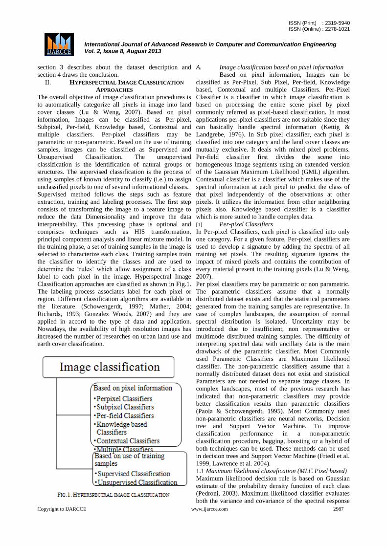
A. Image classification based on pixel information

Based on pixel information, Images can be

classified as Per-Pixel, Sub Pixel, Per-field, Knowledge

based, Contextual and multiple Classifiers. Per-Pixel

Classifier is a classifier in which image classification is

based on processing the entire scene pixel by pixel

commonly referred as pixel-based classification. In most

applications per-pixel classifiers are not suitable since they

can basically handle spectral information (Kettig &

Landgrebe, 1976). In Sub pixel classifier, each pixel is

classified into one category and the land cover classes are

mutually exclusive. It deals with mixed pixel problems.

Per-field classifier first divides the scene into

homogeneous image segments using an extended version

of the Gaussian Maximum Likelihood (GML) algorithm.

Contextual classifier is a classifier which makes use of the

spectral information at each pixel to predict the class of

that pixel independently of the observations at other

pixels. It utilizes the information from other neighboring

pixels also. Knowledge based classifier is a classifier

which is more suited to handle complex data.

[1] Per-pixel Classifiers

In Per-pixel Classifiers, each pixel is classified into only

one category. For a given feature, Per-pixel classifiers are

used to develop a signature by adding the spectra of all

training set pixels. The resulting signature ignores the

impact of mixed pixels and contains the contribution of

every material present in the training pixels (Lu & Weng,

2007).

Per pixel classifiers may be parametric or non parametric.

The parametric classifiers assume that a normally

distributed dataset exists and that the statistical parameters

generated from the training samples are representative. In

case of complex landscapes, the assumption of normal

spectral distribution is isolated. Uncertainty may be

introduced due to insufficient, non representative or

multimode distributed training samples. The difficulty of

interpreting spectral data with ancillary data is the main

drawback of the parametric classifier. Most Commonly

used Parametric Classifiers are Maximum likelihood

classifier. The non-parametric classifiers assume that a

normally distributed dataset does not exist and statistical

Parameters are not needed to separate image classes. In

complex landscapes, most of the previous research has

indicated that non-parametric classifiers may provide

better classification results than parametric classifiers

(Paola & Schowengerdt, 1995). Most Commonly used

non-parametric classifiers are neural networks, Decision

tree and Support Vector Machine. To improve

classification performance in a non-parametric

classification procedure, bagging, boosting or a hybrid of

both techniques can be used. These methods can be used

in decision trees and Support Vector Machine (Friedl et al.

1999, Lawrence et al. 2004).

1.1 Maximum likelihood classification (MLC Pixel based)

Maximum likelihood decision rule is based on Gaussian

estimate of the probability density function of each class

(Pedroni, 2003). Maximum likelihood classifier evaluates

both the variance and covariance of the spectral response





patterns in classifying an unknown pixel. It assumes the

distribution of the cloud of points forming the category

training data to be normally distributed. Under this

assumption, distribution of response pattern can be

described by mean vector and the covariance matrix. From

the given parameters the statistical probability of a given

pixel value can be computed. By computing the

probability of the pixel value, an undefined pixel can be

classified. After evaluating the probability the pixel would

be assigned to the one with highest probability value.

One of the drawbacks in maximum likelihood classifier is

large number of computation required to classify each

pixel. This is true when large number of spectral classes

must be differentiated. The value ^

that maximizes the likelihood is the Maximum

Likelihood Estimate. Often, it is found using calculus;

0d

dL ; 0

2

2

d

Ldmay find some minima and also

need to check boundary values of . The Maximum

likelihood estimation (Eric Zivot, 2001) has the likelihood

functional relation as follows, Let X1,……Xn be the

probability density function where is a (k x1) vector of

parameters that characterize );( ixf

The joint density of the sample is equal to the product of

the marginal densities

)1();();()...;();,....(1

11

n

i

inn xfxfxfxxf

The joint density is an n dimensional function of the data

X1,……Xn given the parameter vector .

1.2 Neural networks classifier

Neural networks (Atli.J et al., 1995) have been

applied successfully in various fields. Neural networks are

networks which needs a long training time but are

relatively fast data classifier. For very high dimensional

data, the training time of a neural network can be very

long and the resulting neural network can be very

complex. This leads to the importance of feature reduction

mechanisms for neural networks. However, few feature

extraction algorithms are available for neural networks.

A neural network is an interconnection of processing units

called neurons. Each neuron receives input signals, xj, j=1,

2…N, which represent the activity at the input are the

momentary frequency of neural impulses derived by

another neuron to this input. In the simplest formal model

of a neuron the output value or the frequency of the neuron

Oi, is often approximated by the function

)2()(1

,

N

j

ijjii xWKO

Where k is a constant and is a non linear function. Wij is

called synaptic efficacies or weights, I is a threshold

A two layer neural network only has one layer of weights

and no hidden neurons, but a multilayer network has many

layers of weights and more than one layer of hidden

neurons (Widrow & Hoff, 1960). In the neural network

approach to pattern recognition the neural network

operates as a black box which receives a set of input

vectors x (observed signals) and produces responses Oi

from the output neurons (i=1..Lwhere L depends on the

number of information classes). A general idea followed in

neural network theory is that the input are either Oi=1, if

neuron I is active for the current input vector x, or Oi=0

(or -1) if it is inactive. The weights are educated through

an adaptive (iterative) training procedure in which a set of

training samples is presented to the input. A neural

network gives an output response for each sample. The

actual output response is compared to the desired response

for the input and the error between the desired output and

the actual output is used to modify the weights in the

neural networks. The training procedure ends when the

error is reduced to a prespecified threshold or it cannot be

minimized any further. Then, all of the data are fed into

the network to perform the classification, and the network

provides at the output the class representation for each

input vector. Neural network classifiers are distortion free

and are very important, especially when parametric

modeling is not applicable.

1.3 Decision trees

Decision tree classifier breaks a complex classification

problem into multiple stages of simpler decision making

processes (Safavian and Landgrebe, 1991). Decision trees

are trees that classify instances by sorting them based on

feature values. Each node in a decision tree represents a

feature in an instance to be classified, and each branch

represents a value that the node can assume (Murthy,

1998). Instances are classified starting at the root node and

sorted based on their feature values.

FIG.2 DECISION TREE

D1

a1

D2

a2

yes

b2

D3

a3

yes

b3

no

c2

D4

a4

yes

b4

no

b1

no

c1

no





TABLE.1 TRAINING SET

D1 D2 D3 D4 Class

a1 a2 a3 a4 yes

a1 a2 a3 b4 yes

a1 b2 a3 a4 yes

a1 b2 b3 b4 no

a1 c2 a3 a4 yes

a1 c2 a3 b4 no

b1 b2 b3 b4 no

c1 b2 b3 b4 no

Fig.2 is an example of a decision tree for the training set of

table 1. Using the decision tree, the instance D1= a1,

D2=b2, D3=a3, D4=b4 would sort to the nodes: D1, D2

and finally D3 which would classify the instance as being

positive (represented by the value yes). The problem of

constructing optimal binary decision trees is a

Nondeterministic Polynomial (NP complete) problem and

thus theoreticians have searched for efficient heuristics for

constructing near optimal decision trees.

The feature that best divides the training data would be

the root node of the tree (Hunt, Martin & Stone, 1966).

Decision trees can be significantly more complex

representation for some concepts due to the replication

problem. A solution to this problem is implementing

complex features at nodes. (Elomaa & Rousu, 1999)

investigated that, use of binary discretization with C4.5

needs half training time by using C4.5 multisplitting.

multisplitting of numerical features doesnot carry any

advantage in prediction accuracy over binary splitting.

Usually Decision trees are univariate since they use splits

based on a single feature at each internal node. Diagonal

partitioning problems cannot be performed by most

decision tree algorithms. The axis of one variable and

parallel to all other axes is orthogonal to the decision of

the instance space. So the resulting regions are all

hyperspectral rectangles.

1.4 Support Vector Machine (SVM)

Specific attention has been dedicated to support vector

machines for the classification of remotely sensed images

recently (Hermes et al., 1999; Roli & Fumera, 2001; Hung

et al., 2002). The interest in growing Support Vector

Machines (Vapnik, 1998; Burges, 1998;

http://www.kernal-Machines.org/tutorial.html) is

confirmed by their successful implementation in numerous

other pattern recognition applications like biomedical

applications (El-Naqa et al., 2002), image compression

(Robinson & Kecman,2003), and three dimensional object

recognition (Pontil & Verri, 1998). These applications are

justified by three reasons: Intrinsic efficiency with respect

to traditional classifiers results in high classification

accuracy, only limited effort is necessary for architecture

design. It is possible to solve the learning problem

according to linearly constrained quadratic programming

methods.

It is a supervised machine learning technique. SVM’s turn

around the notion of a margin either side of the hyper

plane that separates two data classes. Maximizing the

margin and thereby creating the highest possible distance

between the separating hyper plane and the instances on

either side of it has been proven to reduce an upper bound

on the expected generalization error (Vapnik, 1995).

If the training data is linearly separable, then a pair (w, b)

exists such that

)3(1

1

NXallforbXW

PXallforbXW

ii

T

ii

T

With the decision rule given by

)sgn()(, bXWXf T

bw where it is possible to

linearly separate two classes, an optimum separating hyper

plane can be found by minimizing the squared norm of the

separating hyper plane ( Kotsiantis.S.B, 2007).

`The minimization can be setup as a convex quadratic

programming (QP) problem

)4(2

1)(min

,

2wwimise

jw

Subject to LibXWy i

T

i ....1,1)(

In the case of linearly separable data, once the optimum

separating hyper plane is found, data points that lie on its

margin are known as support vector points and the

solution is represented as a linear combination. Some other

data points are ignored.

SVM are binary algorithm, thus made use of error

correcting output coding to reduce a multiclass problem to

a set of binary classification problems (Crammer& Singer,

2002). SVM have often found to provide higher

classification accuracies than other widely used pattern

recognition techniques, such as maximum likelihood and

the multilayer preceptor neural network classifiers. SVM

classification has been applied to a hyperspectral image

with 17 spectral bands from 450nm to 950nm. The ground

resolution is two meters and the image was calibrated to

reflectance by means of empirical line method. SVM

Classification results with reduced false alarms for

thematic classification. Artificial forest areas are difficult

to classify, since trees are small and there is lot of shadows

and it was correctly classified with spectral-angle based

kernel method. Also, fields are classified with

homogeneous area which outfit thematic mapping for land

use (Mercier.G & Lennon,M, 2003).

2 . Sub pixel classifiers

Most classification approaches are based on per-pixel

information in which each pixel is classified into one

category and the land cover classes are mutually exclusive.

Due to the heterogeneity of landscapes and the limitation

in spatial resolution of remote sensing imagery, mixed

pixels are common in medium and coarse spatial

resolution data.





Sub-pixel classification approaches have been developed

to provide a more appropriate representation and accurate

area estimation of land covers than per-pixel approaches

especially when coarse spatial resolution data are used

(Foody & Cox, 1994; Binaghi et al., 1999). A fuzzy

representation in which each location is composed of

multiple and partial memberships of all classes are needed.

The fuzzy-set technique and spectral mixture analysis

classification are the most popular approaches to

overcome mixed pixel problem. One main drawback lies

in the difficulty in assessing accuracy. Most commonly

used classifiers in sub pixel classifications are spectral

unmixing, spectral mixture analysis.

2.1 Spectral unmixing

Hyperspectral unmixing consists of decomposing the

measured pixel reluctances into mixtures of pure spectra.

Assuming the image pixels are linear combinations of pure

materials is very common in the unmixing framework (

Keshava & Mustard, 2002). That is the linear mixing

model considers the spectrum of a mixed pixel as a linear

combination of endmembers, Linear Mixing Model

requires to have known endmember signatures which can

be obtained from a spectral library or by using an End

member Extraction Algorithm (EEA). Spectral unmixing

involves three steps: 1) estimating the number of

individual materials which contribute to the image spectra,

2) identifying the spectra of these materials, 3) unmixing

the image spectra, using different material components.

Spectral unmixing comprises of Endmember Estimation,

Endmember Extraction, Linear Mixture Model and Spatial

Adaptive Unmixing.

2.1.1 End member estimation

The Ground Sample Distance (GSD) of the

imaging sensor and atmospheric conditions affect the

number of end members estimated (Keshava & Mustard,

2002; Gracia.S & Reyes.V, 2010).End members can be

estimated through supervised or unsupervised approaches.

Supervised approaches require the user to count or select

pixels which represent the different materials in the image

(Wu & Chang, 2007). Unsupervised approaches use

dimensionality of the image as the basis for estimating the

number of Endmembers. One such method is PCA which

estimates Ems based on the number of Eigen vectors,

which contains user defined threshold of image variability.

Another recent method is virtual dimensionality (Chang &

Du, 2004) which uses Neyman – Pearson superposition to

compare pixel spectra. Any spectra that are not similar to

another in the image are considered as new material. Any

independent identical distributed noise produces an over

estimate. Another approach uses Bayesian statistics as

threshold for Neyman - Pearson lemma. By using spectral

library, the best representation of each pixel is identified

and then the probability of each identified material being

present is used within the Neyman – Pearson superposition

to more accurately represent the image spectra (Broad.W

& Banerjee, 2009; Eches et al., 2010).

(Messinger et al., 2010) introduced a fully

geometric approach for estimating spatial complexity of an

image based on gram matrix

The gram matrix is defined as

)5()(),()( , jkikjik xxxxxG

Where u is user defined overestimated number of

Endmembers. G is 11 ubyu matrix, 21 ,vv

is the inner product of two vectors 21andvv , ji xx , are

the end member spectra, kx is the particular pixel vector

(mean or origin)

The unique property of gram matrix is that when

the vectors of the gram matrix are linearly dependent, the

determinant is zero.

2.1.2 End Member extraction

After determining the number of endmembers,

the further step is to identify the EMs spectra. There are

two basic approaches: They are Spectral – only EM

extraction and Spectral – Spatial EM extraction (SSEE)

(Canham.K,2011). In spectral only approach, there are

three different approaches. They are Sequential Maximum

Angle Convex Cone (SMACC), Orthogonal Space

Projection (OSP) and Maximum Distance (Max –

D)(Schott.J,2003). In order to find the most distant spectra

and to assign the EMs, spectral-only EM extraction

approach is used.

Spectral spatial EM extraction uses the A Morphological

End member Extractor (AMEE) approach

(Canham.K,2011). SSEE calculates EM spectra from a

group of similar image spectra. There are four steps in

extraction they are global image EMs are found, all image

pixels are projected onto global EMs to find candidate

spectra, the number of candidate spectra are reduced using

spatial constraints, remaining candidate spectra are

ordered.

2.1.3 Linear mixture model (LMM)

In this process the image is unmixed and the individual

Endmember abundance map is calculated (Canham.K,

2011). The HIS spectra T

mxxxX ],...,[ 21 has m

spectral bands, and can be approximated by a linear

combination of N Endmembers, ],...,[ 21 neeeE . The

scalar multiple of each end member is the abundance α.

)7(1

)6(ˆ

1

1

N

i

i

N

i

iieXX

Additive noise causes the sum of all abundance value to

exceed 1. For this reason an emphasis is placed on LMM

that uses non negative constraints only, which is often

referred as Non Negative Least Square (NNLS) (Lawson

& Hanson, 1998). The EMs are found through LMM to be

unlikely to contain a single material, instead each EM is a

non-linear combination of many materials for huge GSD

sensors. This unmixing occurs prior to the reflected light

reaching the sensor. At this scale, a single pixel containing





homogeneous single material is unlikely; however GSD

decreases and spatial resolution increases, it is more likely

for little pixels to contain a single material.

2.1.4 Spatial adaptive unmixing

Local – Local – Global (LLG) is a newer

methodology to improve unmixing errors by finding the

Endmembers of a local area, unmixing that local area

using locally extracted Endmembers and grouping local

Endmembers into global clusters. Figure 3 shows the flow

diagram of Local – Local – Global method (Canham.K,

2011).

Hyper Spectral Image cube is tiled into small spatially

local tiles. After all local tiles are unmixed; the local

Endmembers is clustered together into a reduced group of

global Endmember groups using another interchangeable

component algorithm. NNLS is used for unmixing. Each

local Endmember is assigned to the global Endmember

group to which it is closest. The outputs for LLG are

abundance maps for global EMs, unmixing error images, a

bad pixel map, a map of the number of EMs per tile and a

classification map. The pixels with total abundance values

beyond expectations are identified in bad pixel map. It is

used to compensate for noise causing abundance values to

exceed the sum-to-one constraint ignored in the NNLS

unmixing approach. And checks the sum of abundances

against a user- defined threshold value.

2.2 Spectral mixture analysis

Spectral mixture analysis has been frequently used to

derive sub pixel vegetation information from remotely

sensed imagery in urban areas. The essential assumptions

are the landscape is composed of a few fundamental

components referred to as endmembers each of which is

spectrally distinctive from the others, the spectral

signature for each component is a constant within the

entire spatial extent of analysis and the remotely sensed

signal of a pixel is linearly related to the fractions of

endmember present. The key to successful Spectral

Mixture analysis is appropriate endmembers selection

(Elmore et al., 2000). Selecting endmembers involves

identifying the number of endmembers and their

corresponding spectral signatures.

Hyperspectral sensors take measurements in hundreds of

spectral bands. It is the dimensionality of the data not the

number of bands that determines how many endmembers

can be used in spectral mixture analysis. In a sensitivity

analysis of endmember selection for Spectral mixture

analysis for sub pixel forest cover using Along Track

Scanning Radiometer 2 imagery collected in summer 1997

in central Finland. Spectral Mixture analysis has long been

recognized as an effective method for dealing with mixed

pixel problem. It evaluates each pixel spectrum as a linear

combination of a set of endmember spectra. The output is

in the form of fraction images, with one image for each

endmember spectrum, representing the area proportions of

the endmembers within the pixel. Previous research has

demonstrated SMA is helpful for improving classification

accuracy (kuro.S et al., 1998; Lu et al., 2003).

3 Per- field classifiers

Per-field classifier classifies landuse by predetermined

field boundaries, with an assumption that each field

belongs to a single, homogeneous class (Aplin et al., 1999;

Hill et al., 2002; Erol & Akdeniz, 2005). Per-field

classification is developed to overcome the weakness of

per pixel classification. Per-field classification has the

advantage of allowing incorporation of variety of field

attributes such as size, shape, perimeter of the field as

classification criteria. In Per-field classification, field

boundaries are predetermined. Existing polygon vector

data is utilized, these data usually comes from field

surveys, they provide satisfactory degree of accuracy and

precision (Lobo et al., 1996; Pedley & Curran, 1991; Dean

&Smith, 2003).An alternative way to determine field

boundary is by segmentation techniques and manual

digitizing.

After determination of field boundaries there are several

methods used for classification (Smith &Fuller, 2001;

Janssen & Molenaar, 1995). First method is to utilize field

boundary derive the field attributes. Second method is to

use field boundaries in a post classification stage after per

pixel classification. The other field attributes are field

size(Weiler & Stow, 1991) to characterize urban land use,

(Wit.D & Clevers, 2004) used field areas and shapes to

reassign land classes in post processing stage., (Molenaar

.Z & Gorte,2003) classified different type of land use,(

Fuller et al., 2002) utilized field attributes in both pre-

classification and post classification. In first step, mean

spectral reflectance statistics is within fields and classified

land use. Second step is knowledge based correction to

modify land use classes based on other field statistics such

as class probability, classes of surrounding fields, mean

elevation, modal shape, modal aspect, building area

percentage, building height, and terrestrial cover types.

(Geneleti & Gorte, 2003) demonstrate combine per field

and per-pixel classification to maximize classification

accuracy.

Another method which does not require the use of

Geographical Information Systems (GIS) vector data is

Object-oriented Classification (Walter, 2004). Two stages

of object-oriented Classification are Image Segmentation

and Image Classification. Image segmentation merges

Esti

mate

Nu

mbe

r of

EMs

Extra

ct

EM

spectr

a

Unmix

pixels

using

EMs

Cluster

EMs

into

global

groups

For

m

out

puts

Locally per tile Globally

FIG. 3 LOCAL – LOCAL – GLOBAL METHOD





pixels into objects and classification is performed based on

the objects, instead of an individual pixel. The image

segmentation can be grouped into thresholding, region

based and edge based. In object-oriented classification,

ecognition was performed which is an object based

processing software program. Image Segmentation in

ecognition is a multi-resolution, bottom up, region

merging technique starting with one pixel objects. Image

objects are extracted from the image in a number of

segmentation levels and each subsequent level yields

image objects of a larger average size by combining

objects from a level below, which represents image

information on different scales simultaneously.

The basic idea of object oriented classification is to

classify not only single pixels but groups of pixels that

represent already existing objects in a GIS database. Each

object is described by an n-dimensional feature vector and

classified to the most likely class based on a supervised

maximum likelihood classification. The n-dimensional

feature vector describes the spectral and textural

appearance of the objects. Again the trainings areas are

derived automatically from an existing database (Haralick

& Shapiro, 1985; Fu & Mui, 1981; Pal N.M & Pal S.K,

1993; Walter, 2004). Although Object oriented

classification outperforms the pixel based one, it has some

disadvantages they are the classification accuracy will not

get improved if objects are extracted inaccurately. The

classification error could be accumulated due to error in

both image segmentation and classification process. Once

an object is misclassified, all pixels in this object will be

misclassified.

4. Knowledge based Classifiers

Different kinds of ancillary data, such as digital elevation

model, soil map, housing and temperature are readily

available; they may be incorporated into a classification

procedure in different ways. One approach is to develop

knowledge based classifications based on the spatial

distribution pattern of land cover classes and selected

ancillary data. For example, elevation, slope and aspect are

related to vegetation distribution in mountain regions. A

critical step is to develop the rules that can be used in an

expert system. (Hodgson et al., 2003) summarized three

methods employed to build rules for image classification.

They are explicitly eliciting knowledge from experts,

implicitly extracting variables and rules using cognitive

methods and empirically generating rules from observed

data with automatic induction methods (Kontoes & Rokos,

1996; Hung & Ridd, 2002; Schmidt et al., 2004). GIS

plays an important role in developing knowledge based

classification approaches because of its ability of

managing different sources of data and spatial modeling.

(Mitra.S et.al ,1997) proposed a new scheme of knowledge

based classification and rule generation using a fuzzy

multilayer perceptron. Interms of class apriori

probabilities, knowledge collected from a dataset is

initially encoded among the connection weights. This

encoding includes incorporation of hidden nodes

corresponding to both pattern class and their

complementary regions. In knowledge encoding, let an

interval [Fj1, Fj2] denote the range of feature Fj covered by

class ck. The membership value of the interval as µ([Fj1,

Fj2])=µ (between Fj1 and Fj2) and compute it as shown in

(S.K.Pal and S.Mitra,1992)

µ (between Fj1 and Fj2) = { µ (greater than Fj1 ) * µ (less

than Fj2) }½

(8)

where

µ (greater than Fj1) = { µ (Fj1)} ½

if Fj1≤ Cprop

= { µ (Fj1)} 2

Otherwise

(9)

and

µ (less than Fj2) = { µ (Fj2)} ½

if Fj2

≥ Cprop

= { µ (Fj2)} 2

Otherwise

(10)

Here Cprop denotes cjl, cjm and cjh which represents three

overlapping fuzzy sets low, medium and high as in (S.K

Pal and S.Mitra,1992)

In this a new idea of knowledge encoding among

connection weights of a fuzzy Multiple Layer Perceptron

(MLP) was considered. The techniques involve an

appropriate architecture of fuzzy MLP (S.K Pal and

S.Mitra,1992) in terms of hidden nodes and links. Hence it

is concluded that the speed of learning and classification

performance are better than that obtained with the fuzzy

and MLP

5 Contextual Classifiers

In contextual classifiers, the spatially neighboring pixel

information is used. Contextual classifiers are developed

to cope with the problem of intraclass spectral variations

(Gong and Howarth, 1992). To improve the classification

results, it exploits spatial information among neighboring

pixels (Magnussen et al., 2004). It may use smoothing

techniques, segmentation and neural networks. Most

frequently used approach is Markov random field-based

contextual classifiers (Magnussen et al., 2004).

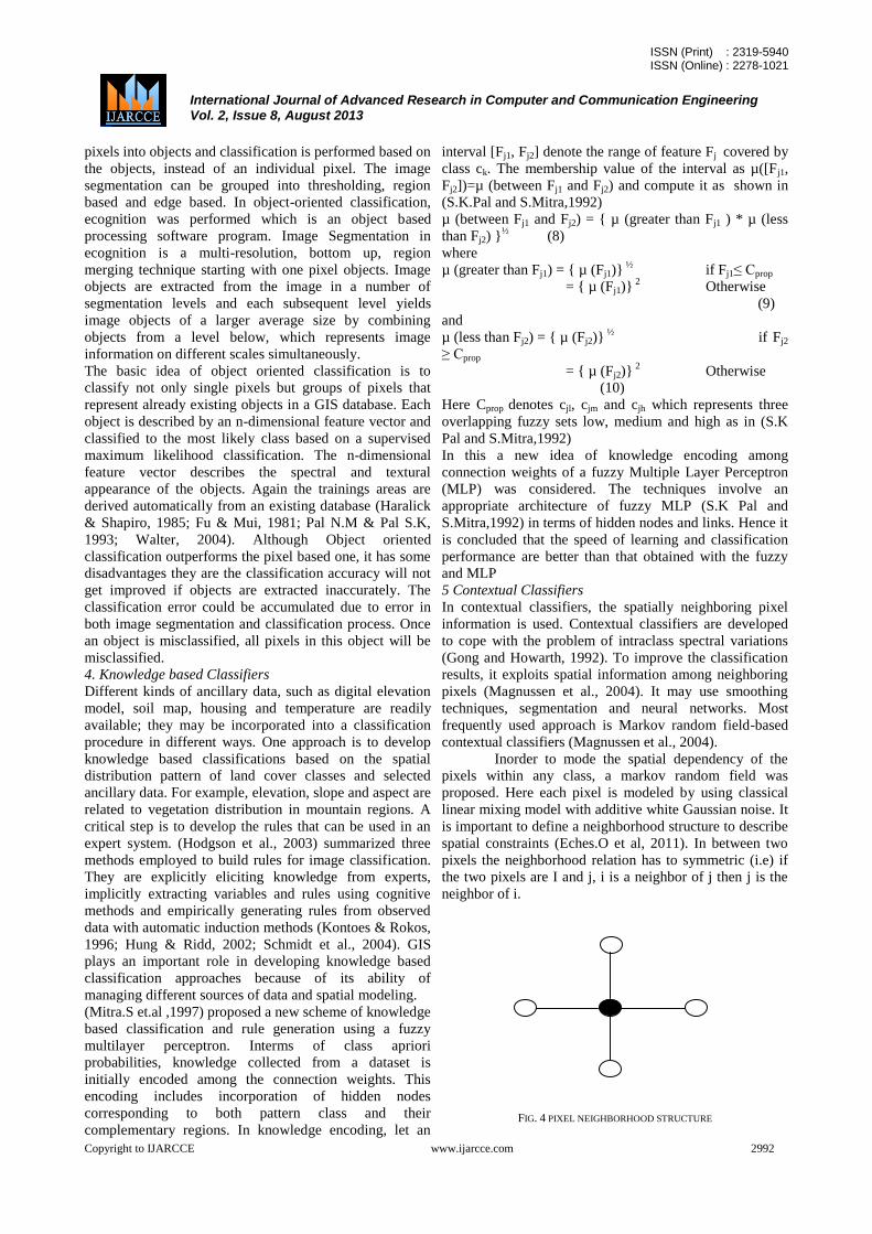
Inorder to mode the spatial dependency of the

pixels within any class, a markov random field was

proposed. Here each pixel is modeled by using classical

linear mixing model with additive white Gaussian noise. It

is important to define a neighborhood structure to describe

spatial constraints (Eches.O et al, 2011). In between two

pixels the neighborhood relation has to symmetric (i.e) if

the two pixels are I and j, i is a neighbor of j then j is the

neighbor of i.

FIG. 4 PIXEL NEIGHBORHOOD STRUCTURE





MRF can be easily defined if the neighborhood structure

has been clearly known. Let us denote Zp as a random

variable associated to the pth pixel of an image of p pixels.

The full set of random variables {Z1,Z2,…Zp} forms a

random field. When the conditional distribution of Zi

given the other pixels Zi only depend on its neighbors and

it is defined to be MRF (i.e)

))(/()/( iZZfiZZf vii V(i) is the neighborhood

structure, };{ ijZZ ii . Neighbors are represented as

white and considered pixel as black.MRF have been used

in image processing community as in (C.Kevrann and F.

Heitz 1995, A.Tonnazini, L.Bedini and E.Salerno, 2006).

Recently hyperspectral community exploited the

advantages of MRFs for hyperspectral image analysis

(R.S.Rand and keenan, 2003)

The new adaptive Bayesian contextual classifier

was developed which combines both the adaptive

procedure (Jackson.Q and Landgrebe.D, 2001) with the

Bayesian contextual iteration conditional modes (ICM).

The joint prior probabilities of the classes of each pixel

and its spatial neighbors are modeled by the markov

random field in Bayesian contextual iteration. While

comparing an MLP classifier with MAP classifier, MAP

performs classification by maximizing the posterior

probability. Here the information is incorporated into the

process of a weighting factor computation and MAP

classification.

6 Multiple classifiers

Different classifiers such as parametric (e.g. maximum

likelihood) and non- parametric classifiers (e.g. neural

network, decision tree) have their own limitation and

strengths (Mather.T.B, 2001; Franklin et al., 2003). When

sufficient training samples are available and the feature of

land covers in a dataset is normally distributed, a

maximum likelihood classifier may yield an accurate

classification result. In contrast, when image data are

anomalously distributed, neural network and decision tree

classifiers may demonstrate a better classification result

(Pal & Mather, 2003 & Lu et al., 2004). Some previous

research has explored different techniques such as

production rule, sum rule, stacked regression methods and

thresholds to combine multiple classification results

(Steele, 2000; Liu et.al, 2004).

B. Image classification based on training samples

Training Samples are classified as Supervised

Classification and Unsupervised Classification. In

supervised classification, it identifies known a priori

through a combination of fieldwork, map analysis as

training sites; the spectral characteristics of these sites are

used to train the classification algorithm for eventual land

cover mapping of the remainder of the image. In

Unsupervised Classification, the computer or algorithm

automatically group pixels with similar spectral

characteristics (means, standard deviations, etc.,) into

unique clusters according to some statistically determined

criteria. The analyst then re-labels and combines the

spectral clusters into information classes.

1.Supervised Classification

In supervised Classification, Land cover classes are

defined. Sufficient reference data are available and used as

training samples (Lu & Weng, 2007). The signatures

generated from the training samples are then used to train

the classifier to classify the spectral data into a thematic

map. Most frequently used supervised classification

approaches are maximum likelihood, decision tree and

neural network. One of the tasks carried out by Intelligent

System is Supervised Classification. A large number of

methods have been developed based on Perceptron based

techniques (i.e) Feed Forward Networks (Kotsiantis.

S.B,2007).

1.1 Feed Forward Networks

Only linearly separable sets are classified by

perceptrons. To separate the input instances into their

correct categories a straight line or plane can be drawn so

that input instances are linearly separable and perceptron

will find a result. All instances are classified properly, if

the instances are not linearly separable. To solve this

problem, multilayered perceptron have been achieved. An

overview of existing work in Artificial Neural Networks

was provided by (Zheng, 2000). Feed Forward Networks

are classified as single layered perceptrons and multi

layered perceptrons.

Single layered perceptron is used for predicting the labels

on the test set. WINNOW (Littlestone & Warmuth, 1994)

is based on the perceptron idea and its updated weights. If

the actual value is one then weights are obtained to be too

low with prediction value zero. Each feature is one,

wi=wiα, where α is a number greater than one called the

promotion parameter. If the actual value is zero, then the

weights are obtained to be too high with the prediction

value one, thus the corresponding weight gets decreased

by setting wi=wiβ where 0<β<1 called the demotion

parameter. One example of exponential update algorithm

is WINNOW. Here the weight of irrelevant features gets

reduced exponentially and a weight of relevant feature

gets increased exponentially. Due to this reason, it was

performed experimentally (Blum, 1997) that WINNOW

adopts the changes in target function.

(Freund & Schapire, 1999) created a new

algorithm called voted perceptron, that stores more

information during training and then generate better

predictions about the test data. List of all prediction

vectors is the information maintained during training that

was generated after each and every mistake. For each

vector, it counts the number of iterations it survives until

the next mistake is performed. This count is referred to as

weight of the prediction vector.

A Multi layered neural network consists of large

number of units (neurons) joined together in a pattern of

connections (Kotsiantis S.B, 2007). Units are usually

segregated into three classes. Input units which receive

information to be processed, the output units which gives

the result, in between them there is a hidden unit. The

network is trained to determine input, output mapping and

the weights of the connections are then fixed and the

network is used to determine the classification of a newer





set of data. During classification the signal from input

units propagates through the net to determine the

activation values at all the output units.

Each input unit has an activation value which

represents a feature outside the set. Every input unit sends

its activation value to each hidden units. Each hidden units

calculates its activation value and this signal is passed to

output unit. Each activation values for receiving units are

calculated to a simple activation function which sums

together the contributions of all sending units (Product of

both the weight of connection between sending and

receiving units and sending units activation value). Proper

determination of the size of the hidden layer is complex

because of an estimation of number of neurons which

leads to poor approximation and generalization

capabilities.

The minimum number of neurons and the number

of instances needed to program a task into feed forward

neural network has been studied in (kon and Plaskota,

2000), (Canargo and Yoneyama, 2001) most commonly

the feed forward neural networks are trained by original

back propagation algorithm. This problem is too slow for

most applications. One approach to speed up the training

rate is to estimate optimal initial weights (Yam and Chow,

2001). Weight elimination algorithm is the another method

for training multilayer feed forward ANN that

automatically drives the appropriate topology and avoid

the problem with over fitting (Weigend et. al., 1991). To

train the weights of neural networks genetic algorithm was

proposed and to determine the architecture of neural

networks (Yen and Lu, 2000) genetic algorithm was

proposed.

1.2 Bayesian Networks

It is a graphical model for probability relations among a

set of variables ( Kotsiantis S.B, 2007). The structure of

this network is a directed acyclic graph; each node in this

graph has one to one relationship with the features. The

arcs represent casual influences among features and lack

of arcs encodes a conditional independencies. A feature is

conditionally independent from its non descendents.

Learning a Bayesian network can be divided into

two tasks, learning of DAG structure and determination of

its parameters. The probabilistic parameters are encoded

into a set of tables, local conditional distribution of each

variable, independencies, joint distribution is constructed

by multiplying these tables. The framework of inducing

Bayesian networks involves known structure and unknown

structure. In the known structure, the structure of the

network is assumed to be correct. Learning the parameters

in the conditional probability tables (CPT) is usually

solved by determining a locally exponential number of

parameters from the data provided. If the network

structure is fixed in nature (Jensen, 1996) each node has an

associated CPT that describes the conditional probability

distribution of that node. They have an inherent limitation

in spite of the remarkable power of Bayesian networks.

This is the computational difficulty of exploring an earlier

unknown network.

(Acid and De Campos, 2003) proposed a new

local search method which uses a different search space

and takes account of the concept of equivalence between

network structures. In this way, efficiency gets improved

due to the reduced search space in no. of different

configuration. The most important feature of Bayesian

network compared to decision trees or neural network is

the possibility of taking prior information into account

about a given problem. In terms of structural relationship

between its features the domain knowledge about the

Bayesian network may take the following forms they are

a) if a node has no parents then the node is root node, b) if

a node h as no children then the node is leaf node, c) the

node is a direct effect of another node, d) a node is not

directly connected to another node, e) two nodes are

independent given a conditional set, f) a node appears

earlier than another node in ordering providing a complete

node ordering.

A Bayesian Network structure was found by

learning conditional independence relationships among the

features of a dataset. One can find the conditional

independence relationships among the features by using a

few statistical tests as constraints to construct a Bayesian

Networks. These algorithms are called CI-based

algorithms or Constraint-based algorithms. For any

structure search procedure based on CI tests, an equivalent

procedure based on maximizing a score can be specified

by (Cowell,2001).Problems found in Bayesian Network

classifiers are they are not suitable for datasets with many

features(Cheng et.al., 2002). Before the induction, the

numerical features are needed to be discretized.

[2] Unsupervised Classification

In Unsupervised Classification Clustering based

algorithms are used to partition the spectral image into a

number of spectral classes based on the statistical

information inherent in the image. No prior definitions of

the classes are used. The analysis is responsible for

labeling and merging the spectral classes into meaningful

classes. The unsupervised classification approaches are

ISODATA and K-means Clustering Algorithm. One of the

methods used in unsupervised classification technique is

ISODATA (Melesse.M.A & Jordan.J.D, 2002) which

uses a maximum- likelihood decision rule to calculate

class. It can be evenly distributed in the data space and

then iteratively clusters the remaining pixels using

Minimum Distance techniques. The pixels get reclassified

and each iteration recalculates the means with respect to

new means. This continues until the no. of pixels in each

class changes by less than a selected pixel.

K- Means clustering (Wagstaff.K et al., 2001) is a

common method used to automatically partition a dataset

into k groups. Select k initial cluster centers and then

iteratively refine them as follows. Here each instance is

assigned to its closest cluster center. Each cluster center Cj

is updated to be the mean. When there is no change in

assignment of instances to clusters this algorithm gets

converged. Unsupervised Methods have produced good

results in (Marson.P, 1993) hyperspectral image

classification. Since unsupervised methods work on the





whole image, they are not sensitive to the number of

labeled samples, but the relationship between clusters and

classes are not ensured. Moreover, a preface feature

selection and extraction step is usually undertaken to

reduce the high input space dimension, which is time-

consuming and needs prior knowledge.

III. DATASET DESCRIPTION

This section describes the various datasets

considered for hyperspectral Image Classifications. These

Image sets were gathered from Airborne Hyperspectral

Sensors. Airborne Hyperspectral Sensors includes

Airborne Visible/infrared Imaging Spectrometer

(AVIRIS), HYmap Imaging Spectrometer

(HYMAP).AVIRIS was developed by NASA with 4m-

20m spatial Resolution, 224 data channels and generates a

vast amount of data. A Fixed Narrow Bandwidth image of

contiguous spectral bands can be collected from

Hyperspectral sensors. Especially at longer wavelengths,

this may cause low SNR (Gianinetto.M & Lechi.G, 2004).

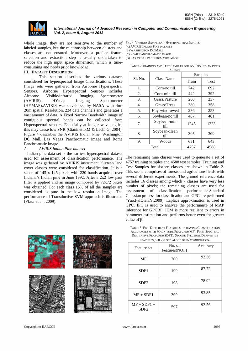
Figure 4 describes the AVIRIS Indian Pine, Washington

DC Mall, Las Vegas Panchromatic image and Rome

Panchromatic image.

A. AVIRIS Indian Pine dataset

Indian pine data set is the earliest hyperspectral dataset

used for assessment of classification performance. The

image was gathered by AVIRIS instrument. Sixteen land

cover classes were considered for classification. It is a

scene of 145 x 145 pixels with 220 bands acquired over

Indiana’s Indian pine in June 1992. After a 2x2 low pass

filter is applied and an image composed by 72x72 pixels

was obtained. For each class 15% of all the samples are

considered as pure in the low resolution image. The

performance of Transductive SVM approach is illustrated

(Plaza et al., 2009).

FIG. 4. VARIOUS SAMPLES OF HYPERSPECTRAL IMAGES.

(A) AVIRIS INDIAN PINE DATASET (B) WASHINGTON DC MALL

(C) ROME PANCHROMATIC IMAGE

(D) LAS VEGAS PANCHROMATIC IMAGE

TABLE.2 TRAINING AND TEST SAMPLES FOR AVIRIS INDIAN PINES

SUBSET

Sl. No. Class Name Samples

Train Test

1. Corn-no till 742 692

2. Corn-min till 442 392

3. Grass/Pasture 260 237

4. Grass/Trees 389 358

5. Hay-windrowed 236 253

6. Soybean-no till 487 481

7. Soybean-min

till 1245 1223

8. Soybean-clean

till 305 309

9. Woods 651 643

Total 4757 4588

The remaining nine classes were used to generate a set of

4757 training samples and 4588 test samples. Training and

Test Samples for sixteen classes are shown in Table 2.

This scene comprises of forests and agriculture fields with

several different experiments. The ground reference data

includes 16 classes among which 7 classes have very less

number of pixels; the remaining classes are used for

assessment of classification performance.Standard

Gaussian process for classification and GPC are performed

(Yao.F&Qian.Y,2009). Laplace approximation is used in

GPC. IPC is used to analyze the performance of MAP

inference for GPCRF. ICM is more resilient to errors in

parameter estimation and performs better even for greater

value of β.

TABLE 3: FIVE DIFFERENT FEATURE SETS HAVING CLASSIFICATION

ACCURACIES WITH MAGNITUDE FEATURES(MF), FIRST SPECTRAL

DERIVATIVE FEATURES(SDF1), SECOND SPECTRAL DERIVATIVE

FEATURES(SDF2) USED ALONE OR IN COMBINATION.

Feature set No. of

Features(NOF) Accuracy

MF 200 92.56

SDF1 199 87.72

SDF2 198 78.92

MF + SDF1 399 93.85

MF + SDF1 +

SDF2 597

92.56





Table 3 shows SVM Classification accuracy results if

Magnitude Features(MF) are used only, First Spectral

Derivative Features(SDF1) are used only, Second Spectral

Derivative Features(SDF2) are used only, all magnitude

features are fused with first spectral derivative

features(MF+SDF1+SDF2). Low Classification accuracy

was achieved in spectral derivative features compared to

magnitude features. The Classification accuracy can be

improved by fusing spectral derivative features with

magnitude features. Further, the performance to the second

level is reduced while fusing magnitude features with

second spectral derivative features (Demir.B, 2008).

In the case of feature extraction, the classification

accuracy can be evaluated as follows. In three different

feature sets and different proportions, combinations of

transformed features, Principal Component Analysis was

performed separately to obtain total number of desired

features by using SVM Classification.

Table 4 shows maximum classification accuracies.

Combining Magnitude features with first spectral

derivative features gives improved classification accuracy.

Further by combining second spectral derivative features

improve the classification accuracy( Demir.B , 2008).

TABLE 4: CLASSIFICATION ACCURACIES OBTAINED USING MAGNITUDE

FEATURES (MF), NUMBER OF FEATURES (NOF)

NOF MF MF +

SDF1

MF+SDF1 +

SDF2

10 86.79 87.61 87.61

15 88.77 88.77 88.84

20 89.03 89.36 89.36

25 87.61 89.38 89.66

30 85.54 87.68 87.68

35 83.79 86.70 86.70

40 83.06 85.22 85.52

B. Washington DC Mall

Another dataset is a part of an airborne hyperspectral

data over Washington DC mall collected by HYDICE

scanner. It is a scene of 500 x 307 pixels and consists of

210 bands from 0.4 to 2.4 m region of the visible and

infrared spectrum(Yao.F&Qian.Y,2009). During analysis

the water absorption bands are removed and the remaining

191 bands are used. There are 7 classes composed of

water, vegetation, man-made structures and shadow. The

testing and training samples can be manually selected by

visual inspection with the aid of a SAR image and digital

elevation data for the same scene because of its high

spatial resolution. The training and testing samples

available for this image are listed in Table 5.

TABLE.5 TRAINING AND TEST SAMPLES FOR WASHINGTON DC MALL

Sl. No. Class

Name

Training Testing

1. Roads 55 892

2. Grasses 57 910

3. Shadows 50 567

4. Trails 46 623

5. Roofs 52 1123

Total 260 4115

TABLE.6 ANALYSIS OF THE STABILITY OF OVERALL CLASSIFICATION

ACCURACY OF WASHINGTON DC MALL DATASET.

Kernal Parameter

Range Mean Variance

Linear σd €[1.00,1.15] 85.64 % 0.88 %

Rational

Quadratic

l € [2.70,2.72]

α € [7.38,7.40]

88.55 %

1.01 %

Squared

Exponential

l € [2.20,2.23]

σf € [0.8,1.1] 88.90 % 0.86 %

From the table.6, it is seen that Gaussian Process

Classifier (GPC) with squared exponential kernel function

outperformed GPC with Linear kernel in accuracy and

stability of classification. When the number of bands

selected in classification is much less than the number of

all bands, GP gets higher classification accuracy fast at the

same time accuracy drops a little (Yao.F& Qian.Y,2009).

C. Las Vegas Panchromatic image

The Las Vegas scene comprises regular Crisscrossed roads

and buildings characterized by similar heights but different

dimensions, from small residential houses to large

commercial buildings (Tuia.D et.al, 2009). Eleven

different surfaces of interest have been recognized, paying

special attention to the specific peculiarities of each scene.

For this test case, the goal was to distinguish the different

use of the asphalted surfaces which included residential

roads, highways and parking areas. A reference ground

survey of 373023 pixels has been randomly split into the

following: a training set of 30000 pixels, a validation set

of 25000 pixels and a test set of 318023 pixels. The

training and testing samples available for this image are

listed in Table 7.

TABLE.7 TRAINING AND TEST SAMPLES FOR LAS VEGAS DATASET

Sl.

No.

Class Name Training Testing

1. Residential 7066 74553

2. Commercial 1816 19485





3. Road 6089 65068

4. Highway 2858 30220

5. Parking lots 2291 23990

6. Short veg. 1815 19090

7. Trees 1006 11157

8. Soil 1484 15670

9. Water 152 1227

10. Drainage 1098 12224

11. Bare soil 4325 45339

Total 30000 318023

TABLE.8 CLASSIFICATION ACCURACY LAS VEGAS PANCHROMATIC

IMAGE

Class OC-

OCR

RFE-

33

RFE-

29

RFE-

24

RFE-

15 PCA

Residential 96.10 96.15 96.82 96.71 97.36 89.19

Commercial 97.41 97.38 97.13 97.10 96.52 97.78

Road 97.11 97.06 97.26 97.30 97.34 95.19

Highway 98.31 98.25 98.14 98.30 97.94 92.67

Parking lots 91.90 92.03 91.68 91.71 90.59 87.28

Short Vegetation

92.02 92.37 92.36 92.72 91.22 82.84

Trees 87.26 87.64 87.42 88.04 84.77 74.42

Soil 89.68 89.98 88.68 89.09 86.59 84.92

Water 94.79 94.79 93.49 93.49 90.47 88.16

Drainage

Channel 97.23 97.19 97.78 97.48 96.49 94.61

Bare soil 99.52 99.52 99.35 99.38 98.90 98.31

Overall

accuracy 95.93 95.98 96.05 96.11 95.67 90.10

Kappa index 0.952 0.953 0.954 0.955 0.949 0.901

Table.8 shows small increase in the accuracy.

SVM is robust to the problems of dimensionality. Only

features from OCR set was removed during first iteration

(RFE-33, RFE-29). Small scale at this stage

D. Rome Panchromatic image

This Scene consists of older buildings to the upper right

and newer buildings such as apartment blocks in the lower

left the selection of the classes for the scene of Rome was

made to investigate the potential of discriminating

between structures with different heights including

buildings, apartment blocks and towers. (Tuia.D et.al

2009). The surfaces of interest were roads, trees, short

vegetation, soil and peculiar railway in the middle of the

scene for a total of nine classes. A reference ground survey

of 775411 labeled pixels was created. In Complexity of

the scene and of the significant overlap of the classes,

50000 pixels have been retained, 30000 have been used

for model selection and the remaining 695411 have been

used for test. The training and testing samples available

for this image are listed in Table 9. TABLE.9 TRAINING AND TEST SAMPLES FOR ROME PANCHROMATIC

IMAGE DATASET

Sl. No. Class Name Training Testing

1. Buildings 11646 162613

2. Apartment

Blocks

7033 98464

3. Road 10645 146676

4. Railway 1049 14373

5. Vegetation 4408 62465

6. Trees 5883 81465

7. Soil 929 13562

8. Towers 3101 43008

9. Bare soil 5306 72785

Total 50000 695411

TABLE.10 CLASSIFICATION ACCURACY ROME PANCHROMATIC IMAGE

Class OC-OCR RFE-33 RFE-29 RFE-12 PCA

Buildings 89.33 91.21 90.52 87.90 70..82

Blocks 80.80 79.56 79.65 77.62 64.95

Roads 89.39 88.95 89.03 87.02 51.64

Railway 94.98 94.94 94.69 93.93 80.29

Vegetation 84.80 85.26 85.48 82.20 74.42

Trees 78.93 80.26 79.98 78.31 37.70

Bare soil 95.29 95.16 95.12 93.96 83.39

Soil 86.54 86.58 86.09 84.63 86.01

Tower 77.79 72.98 73.87 73.50 70.92

Overall accuracy 86.48 86.54 86.43 84.43 64.10

Kappa index 0.839 0.840 0.838 0.815 0.57

Table.10 shows In RFE-33, the best result was

achieved having overall accuracy of 86.54% with a related

kappa index of 0.840 OC-OCR is optimal in terms of

classification accuracy.

IV. CONCLUSION

Hyperspectral Image Classification has made great

improvement in the development and use of recent

classification algorithms. It uses multiple features such as

spectral, spatial, multitemporal and multi sensor

information and incorporation of additional data into

classification procedures such as soil, road, vegetation and

census data. Accuracy verifications are done based on

error matrix and fuzzy approaches. The most important

factors in classification accuracy are uncertainty and error

propagation chain. Identifying the weakest links in the

chain and then reducing the uncertainties are vital for

improvement of classification accuracy.

Classification algorithms can be per-pixel, sub

pixel, per-field, Contextual and multiple Classifiers. Per-

pixel classification is still mainly used in practice. But, the

accuracy may not meet the necessity because of the impact

of the mixed pixel problem and may realize higher

accuracy for medium and coarse spatial resolution images.

For fine spatial resolution data, although mixed pixels are

reduced, the spectral variation within land classes may

decrease the classification accuracy. Per-field

classification approaches are most optimal for fine spatial

resolution data. In many cases, machine learning

approaches also provide a better classification result than

Maximum Likelihood classifier because of some tradeoffs

exist in classification accuracy, time consumption and

computing resources.

When using multisource data such as

combination of spectral signatures, texture, context

information and additional data, advanced non-parametric

classifiers such as neural network, decision making and

knowledge based classification maybe more suitable to

handle these complex data processes and thus gained

increasing awareness in the remote sensing community in





recent years. Valuable use of multiple features of remotely

sensed data and the selection of a proper classification

method are especially significant for improving

classification accuracy. More research is needed to

identify and reduce uncertainties in the image processing

to improve classification accuracy. The availability of high

quality remotely sensed image, data, design of good

classification procedure and the analysis skills are really

important. Combination of the classifiers has exposed best

results in classification accuracy.

REFERENCES

[1] Acid ,S. and de Campos ,L.M.( 2003), searching for Bayesian Network structure in the space of Restricted Acyclic Partially Directed

Graphs. Journal of Artificial Intelligence Research, 18, 445-490.

[2] Aplin,P. Atkinson ,M.P,Curran,J.P., (1999), Fine spatial resolution simulated satellite sensor imagery for land cover mapping in

the united kingdom, Remote sensing of environment, 66, 206- 216

[3] Binaghi, E. Brivio, P.A, Ghezzi.P and Rampini.A, (1999), A Fuzzy set accuracy assessment of Soft Classification. Pattern Recognition

Letters, 20,935-948

[4] Blum.A,(1997), Empirical Support for Winnow and Weighted-Majority Algorithms: Results on a Calendar Scheduling Domain,

Machine Learning,26, 5-23

[5] Burges C.J.C, (1998), A tutorial on Support Vector Machines for Pattern Recognition Data Mining Knowledge Discov., 2, 121-167.

[6] Canargo and Yoneyama, (2001), Specification of Training Sets

and the Number of Hidden Neurons for Multilayer Perceptrons. Neural Computations,13, 2673-2680

[7] Canham.K , Schlamm,A Basener,B Messinger,D (2011),High Spatial Resolution Hyperspectral Spatially Adaptive Endmember

Selection and Spectral Unmixing,8048,

[8] Chang.C.I, and Du.Q, (2004),Estimation of number of spectrally distinct signal sources in hyperspectral imagery, geosciences and remote

sensing, IEEE Trans., 608-619

[9] Cheng,J. Greiner,R. Kelly,J. Bell,D. Liu,W.(2002), Learning Bayesian networks for data: An information-theory based approach,

Artificial Intelligence,137,43-90

[10] Cowell,R.G. (2001), Conditions under which Conditional Independence and Scoring methods leads to Identical Selection of

Bayesian Network Models. Proc.17th International Conference on

Uncertainty in Artificial Intelligence [11] Crammer,K. & Singer,Y. (2002), On the learn ability and design

of output codes for multiclass problems and machine learning, 47, 201-

233 [12] Dean ,A. and Smith ,G. (2003), An evaluation of per pixel land

cover mapping using maximum likelihood class probabilities,

International Journal of Remote Sensing, 24, 2905 – 2920 [13] Demir.B and Erturk,S.(2008),Spectral Magnitude spectral

derivative feature fusion for improved classification of hyperspectral

images, IGARSS, 1020-1023 [14] Eches,O. Dobigeon,N and Tourneret,J. (2011) , Enhancing

hyperspectral image unmixing with with spatial constraints, IEEE

Transaction on Geoscience and Remote Sensing,(1-9). [15] Elmore ,J. Mustard,J.F, Manning,S .J,. Lobell,D.B ( 2000),

Quantifying vegetation change in semi arid environments; precision and

accuracy of spectral mixture analysis and the normalized difference vegetation index, Remote sensing of Environment, 73, 87 – 102

[16] El-Naqa.I , Yongi Y, Wernick M.N, Galatsanos .P.N,

Nishikawa.M.R ,(2002), A support vector machine approach for detection of micro calcifications, IEEE Transactions on medical

Image,21,12, 1552-1563.

[17] Elomaa.T and Rousu.J, (1999), General and Efficient Multisplitting of Numerical Attributes. Machine Learning, 36,201-244

[18] Erol.H and Akdeniz.F, (2005), A per field classification method

based on mixture distribution models and an application to land sat thematic mapper data, International Journal of Remote sensing, 26, 1229

– 1244

[19] Foody G.M, Cox D.P., (1994), Subpixel landcover composition estimation using a linear mixture model and fuzzy membership functions,

Int. Remote sensing, 15, 619- 631

[20] Franklin .J, Stuart R.Phinn, Curtis E.Woodcock, John Rogan.,

(2003), Rationale and conceptual framework for classification approaches to assess forest resources and properties, Remote sensing of

forest Environments concepts and case studies, 279 – 300

[21] Freund .Y & Schapire, R. ( 1999) , Large Margin Classification using the Perceptron Algorithm, Machine Learning, 37, 277-296

[22] Friedl, M.A, Brodley C.E, and Strahler A.H ,(1999), Maximizing land cover classification accuracies produced by decision trees at

continental to global scales, IEEE Transactions on Geoscience and

Remote Sensing, 37,969-977. [23] Fu.M and C.Mui,( 1981), A survey on Image segmentation,

pattern recognition, 13, 3 – 16

[24] Fuller, R., Smith, G., Sanderson, J., Hill, R. and Thomson, A.,( 2002), The UK Land Cover Map 2000: Construction of a parcel-based

vector map from satellite images. The Cartographic Journal, 39, 15–25.

[25] Geneleti.D and Gorte.B, (2003), A method for object oriented land cover classification combining land set TM data and aerial photographs,

International Journal of remote sensing, 24, 1273 – 1286

[26] Gianinetto.M and Lechi,G (2004),The Development of Superspectral approaches for the improvement of Land cover

classification, IEEE Transactions on Geoscience & Remote Sensing, 42.

[27] Goetz.A.F.H., Vane, G.Solomon, J.E &Rock B.N, (1985) ,Imaging spectrometry for earth remote sensing science, 228 ,1147-1153

[28] Gong.P and Howaeth P.J, (1992), Frequency-based contextual

classification and gray level vector reduction for land use identification, Photogrammetric Engineering and Remote sensing,,58,423-437.

[29] Gonzalez R.C Woods.R.A, (2007), Digital Image Processing,

Prentice Hall, , 976 [30] Gracia.A,S and Velez – Reyes.M,(2010), Understanding the

impact of spatial resolution in unmixing of hyperspectral images,

algorithms and technologies for multispectral, hyperspectral and ultra spectral imagery, XVI7695(1), 1-12.

[31] Haralick R.M and Shapiro L.G, (1985), Image segmentation

techniques, computer vision graphics and image processing, 29, 100 – 132

[32] Hermes .L, D.Frieauff, J.Puzicha and J.M Buhmann, , (1999).

Support Vector Machines for land usage classification in land set TM imagery, in Proc. IGARSS, Hamburg, Germany, 348-350

[33] Hill, R., Smith, G., Fuller, R. and Veitch, N.,(2002), Landscape

modelling using Integrated airborne multispectral and laser scanning

data, International Journal of Remote Sensing, 23, 2327–2334.

[34] Hodgson. M.E , John R.Jensen, Jason A.Tullis, Kevin .D.Riordan

and Clerk M.Archer, (2003), Synergistic use Lidar and color Arial photography for mapping urban parcel imperviousness, Photogrammetric

Engineering and remote sensing, 69, 973 - 980

[35] Hung.M and Ridd. M.K,( 2002), A sub pixel classifier for urban land cover mapping based on a maximum likelihood approach and expert

system rules, Photogrammetric engineering and remote sensing, 68, 1173

- 1180 [36] Hunt.E.Martin.J. &Stone.P, (1966), Experiments in Induction,

Newyork, Academic Press.

[37] Jackson.Q and Landgrebe,D.(2002), Adaptive Bayesian Contextural Classification Based on Markov Random Fields, IEEE

Transactions on Geoscience and Remote Sensing, 40, 11, 2454-2463.

[38] Janssen L.P and Molenaar M.,(1995). Terrain Objects, their dynamics and their monitoring integration of GIS and remote sensing.

IEEE Transactions on Geoscience & Remote Sensing, 33, 749-758. [39] Jensen.F, (1996), An Introduction to Bayesian Networks,Springer.

[40] Atli,J. Benediktsson, Johan Nes R, Arnason,S.K

(1995),Classification and feature extraction of AVIRIS data, IEEE Trans. On Geo Science and Remote Sensing, 33,

[41] Keshava.N & J.F.Mustard, (2002), Spectral Unmixing, IEEE

Signal Processing. 19,44-57. [42] Kettig.R.L and Landgrebe.D.A, (1976), Classification of

multispectral image data by extraction and classification of homogenous

objects, IEEE transactions on Geoscience Electronics, 19-26. [43] Kevrann.C , Heitz.F, (1995), A markov random field model-

based approach to unsupervised texture segmentation using local and

global statistics’, IEEE Transaction Image Processing, 4, 6, 856-862 [44] kon and Plaskota,(2000), Information Complexity of neural

networks , Neural Networks,13 ,365-375.

[45] Kontoes. C.C., Rokos.D, (1996), The integration of spatial context information in an experimental knowledge based system and the

supervised relaxation algorithm: two successful approaches to improving





SPOT-XS classification, International journal of remote sensing, 17,

3093 - 3106 [46] Kotsiantis.S.B, (2007), Supervised Machine Learning: A Review

of Classification Techniques, Informatica 3, 249-268.

[47] Lawrence R,Bunn.A, Powell.s and Zmabon .M, (2004),Classification of Remotely Sensed imagery using stochastic

gradient boosting as a refinement of classification tree analysis. Remote Sensing of Environment, 90,331-336.

[48] Lawson C.L and Hanson R.J, (1998), solving least squares

problems, Society of industrial and applied mathematics, 160 – 164 [49] Littlestone.N, Warmuth.M,(1994), The weighted Majority

algorithm. Information and computation, 108(2):212-261

[50] Liu.W, Sucharita Gopal and Curtis E.Woodcock, (2004), Uncertainty and confidence in land cover classification using a hybrid

classifier approach, photogrammetric Engineering and Remote Sensing,

70, 963 – 972. [51] Lobo.A, Chic.O and Casterad.A, (1996), Classification of

Mediterranean crops with multisensory data pixel versus per – object

statistics and image segmentation, International journal of remote sensing, 17, 2385 – 2400

[52] Lu .D & Weng.Q, (2007), A Survey of Image Classification

methods and techniques for improving classification Performance, International Journal of Remote Sensing, 28, 5, 823-870.

[53] Lu .D, (2004), Comparison of land cover classification methods in

the Brazilian Amazon basin, Photogrammatic Engineering and remote sensing of Environment, 74, 545 - 556

[54] Lu.D, Moran,E. Batistella,M. (2003), Linear mixture model

applied to Amazonian vegetation classification, Remote sensing of Environment, 87, 456 – 469

[55] Magnussen.S, Boudewyn.P and Wulder.M, (2004), Contextual

Classification of Landsat TM images to forest inventory cover types. International Journal of Remote Sensing. 24 2421-2440

[56] Marson.P and W.Pieczynski, (1993), SEM algorithm and

unsupervised statistical segmentation of satellite images, IEEE Transactions on Geoscience and Remote sensing, 31, 618-633.

[57] Mather P M, (2004), Computer processing for remotely sensed

images: an introduction, Wiley, Newyork, 442 [58] Mather T.B.P.M, (2001), Classification methods for remotely

sensed data, Newyork: Taylor and Francis Inc.,

[59] Melesse .M. A and Jordan,J.D, (2002), Photogrammetric

Engineering and Remote Sensing, 68.

[60] Melgani.F and L. Bruzzone,(2004), Classification of hyperspectral

remote sensing images with support vector machines, IEEE transaction on geo science and remote sensing, 42, 1778 - 1790

[61] Mercier.,G.and Lennon,M. SVM for hyperspectral image

classification with spectral-based kernels, IEEE, 6, 7803-7930. [62] Mitra,S. Rajat.K.De and Pal,S.K (1997),Knowledge- Based Fuzzy

MLP for Classification and Rule Generation, IEEE Transactions on

neural networks,8,1338-1350 [63] Murthy,(1998), Automatic Construction of Decision Trees from

Data. A Multi-Disciplinary Survey, Data Mining & Knowledge, 345-389

[64] Pal N.R and Pal S.K, (1993),A review on image segmentation techniques. Pattern recognition, 26, 1277 – 1294

[65] Pal S.K and Mandal D.P, (1992), Linguistic recognition system

based on appropriate reasoning, Inform., Science, 61,135-161 [66] Pal S.K and Mitra.S, (1992), Multilayer perceptron fuzzy sets and

classification, IEEE Transactions on Neural networks,3,683-697 [67] Pal.M & Mather P.M, (2003), An Assessment of the effectiveness

of decision tree methods for land cover Classification. Remote sensing of

Environment, 86, 554-565. [68] Paola J.D and Schowengerdt R.A,(1995), A review and analysis

of back propagation neural networks for classification of remotely sensed

multispectral imagery, Int. journal of Remote sensing, 16, 303-308 [69] Pedley,M.I and Curran P.J., (1991), Per field Classification an

example using SPOT HRV imagery International Journal of Remote

Sensing,12 , 2181-2192. [70] Perroni. L,(2003), Improved Classification of Landsat Thematic

Mapper data using modified priori Probabilities in large and complex

landscapes, International Journal of Remote Sensing, 24,91-113 [71] Plaza .A, Benediktsson,J.A, Boardman,J.W, Brazile,J.

Bruzzone,L. Camps-Valls,G. Chanussot,J Fauvel,M. Gamba,P.

Gualtieri,A. Marcoccini,M. Tilton,J.C. Trianni,G. et.al, (2009), Recent Advances in techniques for hyperspectral image processing, Remote

sensing of environment,113, S110-S122.

[72] Pontil.M, Verri.A (1998), Support Vector Machines for 3D Object

Recognition, IEEE Transaction pattern Anal. Machine Intel, 20, 637-646. [73] Rand.R.S and keenan, (2003), spatially smooth partitioning of

hyperspectral imagery using spectral, spatial measures of disparity, IEEE

Trans. Geo science and remote sensing, 41, 6, 1479 – 1490 [74] Richards.J.A, (1993), Remote sensing digital image analysis An

introduction, Berlin, Springer-verlag, , 340 [75] Robinson, Kecman.V, (2003),Combining Support Vector Machine

learning with the discrete cosine transform in Image Compression, IEEE

Trans. Neural Networks, 14, 950-958. [76] Roli.F and G.Fumera,(2001), support vector machines for remote

sensing, Image Classification, Proc. SPIE, 4170, 160-166

[77] Safavian.S.R and D. Landgrebe, (1991), A Survey of decision tree Classifier Methodology, IEEE Transaction on Systems, Man and

Cybernetics ,660-674.

[78] Schmidt K.S, Skidmore.A.K, Kloosterman, Van Oosten.H, Kumar .L and Janssen J.A.M et.al., (2004), mapping coastal vegetation using an

expert system and hyperspectral imagery, Photogrammetric Engineering

and remote sensing, 70, 703 - 715 [79] Schott.J.R, Lee.K, Raqueno. R.V, Hoffmann G.D, Healey.G,

(2003), A Subpixel target detection technique based on the invariant

approach, AVIRIS, AVIRIS workshop, Pasadena, California, United States.

[80] Schowengerdt.R.A (1997), Remote sensing models and methods

for image processing, London, Academic Press, , 521 [81] Set of tutorials on SVMs and kernel methods [online]-Available:

http://www.Kernal-Machines.org/ tutorial.html.

[82] Shimabu kuro.Y.E, Batista G.T, Mello E.M, Moreira.J.C and Duarte .V., (1998), Using shade fraction image segmentation to evaluate

deforestation in landsat thematic images of the Amazon region,

international journal of remote sensing, 19, 3,535 - 541 [83] Smith and Fuller, (2001), An integrated approach to land cover

classification - An example in the island of Jersey, International Journal

of remote sensing, 22, 3123 – 3142 [84] Starks,S.A. and EI Paso,(2001), Internal and fuzzy methods in

remote sensing and satellite image processing, 18 ,2019-2022

[85] Steele B.M, (2000), Combining multiple classifiers: an application using spatial and remotely sensed information for land cover type

mapping, remote sensing , 70, 545 – 556

[86] Tonazzini.A, Bedini.L & Salerno.E,(2006), A Markov model

for blind image separation by a mean field EM algorithm, IEEE

Transaction Image Processing, 15, 2 , 473-481

[87] Tuia,D. Pacifici,F. Kanevski,M and Emery,W.J, (2009), Classification of very High Spatial Resolution Imagery Using

Mathematical Morphology and Support Vector Machines, IEEE

Transactions on Remote Sensing,47,11,3866-3879 [88] Vapnik,(1995),The nature of Statistical learning theory, Newyork.

[89] Vapnik. V.N, (1998), Statistical Learning Theory, Newyork,

Wiley. [90] Wagstaff,K. and Cardie,C. (2001),Constrained K-means clustering

with background knowledge, Proceedings of the eighteenth international

conference on machine learning , 577 – 584. [91] Walter V, (2004),Object-based Classification of remote sensing

data for change detection. ISPRS Journal of Photogrammetry & Remote

sensing,58,225-238. [92] Water.J B and Banerjee.A, A Neyman (2009) ,Pearson approach

to estimating the number of end members, Geoscience and Remote sensing symposium, IEEE Intl. IGARSS, 14, 696

[93] Weigend A.S, Rumelhart. D.E, Hubernman B.A,(1991),

Generalization by weight elimination with application to forecasting , In Advances in Neural Information Processing Systems,3, 875-882

[94] Weiler, R. and Stow, D., (1991) , Spatial analysis of land cover

patterns and corresponding remotely-sensed image brightness. International Journal of Remote Sensing, 12, 2237–2257.

[95] Widrow.B and M.E Hoff, (1960), Adaptive switching circuits,

IRE Wescon conv Rec. Newyork,96-104 [96] Wit,D.A. and Clevers, J., (2004), Efficiency and accuracy of per-

field classification for operational crop mapping. International Journal of

Remote Sensing, 25, 4091–4112. [97] Wu. C.C and Chang. C.I, (2007),Does an end member set really

yield maximum simplex volume, in geosciences and remote sensing

symposium, IGARSS, IEEE Int. journal, 3814, 23-28





[98] Yam and Chow, (2001),Feed forward Networks Training Speed

Enhancement by Optimal Initialization of the Synaptic Coefficients, IEEE Transactions on Neural Networks, 12, 430-434

[99] Yao.F and Qian,Y.( 2009), Band Selection based Gaussian

processes for Hyperspectral Remote Sensing Images Classification, IEEE, ICIP ,2845-2848

[100] Yen and Lu, (2000), Hierarchial genetic algorithm based neural networks design, IEEE Symbosium on combinations of Evolutionary

Computation and Neural Networks, 168-175

[101] Zhan Q, Molenaar and Gorte.B, (2000), Urban land use classes with fuzzy membership and classification based on integration of remote

sensing and GIS, International archives of Photogrammetry and remote

sensing, 33,1751 – 1759 [102] Ziemann A.K, Messinger D.W and Basener (2010), W.F Iterative

convex hull volume estimation in hyperspectral imagery for change

detection, in algorithms for multispectral, hyperspectral and ultra spectral imagery, XVI, SPIE

[103] Zivot.E, (2009), Maximum likelihood Estimation.

Documents

A Survey of Hyperspectral Image Classification in -