A Survey of Multilinear Subspace Learning

for Tensor Data

Haiping Lua ∗, K. N. Plataniotisb, A. N. Venetsanopoulosb,c

aInstitute for Infocomm Research, Agency for Science, Technology and Research,#21-01 Connexis (South Tower), 1 Fusionopolis Way, Singapore 138632

bThe Edward S. Rogers Sr. Department of Electrical and Computer Engineering,University of Toronto, 10 King’s College Road, Toronto, ON, M5A 3G4, CanadacDepartment of Electrical and Computer Engineering, Ryerson University, 350

Victoria Street, Toronto, ON, M5B 2K3, Canada

Abstract

Increasingly large amount of multidimensional data are being generated on a dailybasis in many applications. This leads to a strong demand for learning algorithmsto extract useful information from these massive data. This paper surveys the fieldof multilinear subspace learning (MSL) for dimensionality reduction of multidimen-sional data directly from their tensorial representations. It discusses the centralissues of MSL, including establishing the foundations of the field via multilinearprojections, formulating a unifying MSL framework for systematic treatment of theproblem, examining the algorithmic aspects of typical MSL solutions, and catego-rizing both unsupervised and supervised MSL algorithms into taxonomies. Lastly,the paper summarizes a wide range of MSL applications and concludes with per-spectives on future research directions.

Key words: Subspace learning, dimensionality reduction, feature extraction,multidimensional data, tensor, multilinear, survey, taxonomy

Please cite:Haiping Lu, K. N. Plataniotis and A. N. Venetsanopoulos, “A Survey of Mul-tilinear Subspace Learning for Tensor Data”, Pattern Recognition, vol. 44, no.7, pp. 1540-1551, Jul. 2011.

BibTeX:http://www.dsp.utoronto.ca/~haiping/BibTeX/MSLSurvey2011.bib

∗ Corresponding author. Tel: (65)64082527; Fax: (65)67761378 Email:hplu@ieee.org

Article published in Pattern Recognition 44 (2011) 1540–1551

1 Introduction

With the advances in data collection and storage capabilities, massive multidi-mensional data are being generated on a daily basis in a wide range of emerg-ing applications, and learning algorithms for knowledge extraction from thesedata are becoming more and more important. Two-dimensional (2D) data in-clude gray-level images in computer vision and pattern recognition [1–4], mul-tichannel EEG signals in biomedical engineering [5, 6], and gene expressiondata in bioinformatics [7]. Three-dimensional (3D) data include 3D objects ingeneric object recognition [8], hyperspectral cube in remote sensing [9], andgray-level video sequences in activity or gesture recognition for surveillance orhuman-computer interaction (HCI) [10,11]. There are also many multidimen-sional signals in medical image analysis [12], content-based retrieval [1, 13],and space-time super-resolution [14] for digital cameras with limited spatialand temporal resolution. In addition, many streaming data and mining dataare frequently organized as third-order tensors [15–17]. Data in environmen-tal sensor monitoring are often organized in three modes of time, location,and type [17]. Data in social network analysis are usually organized in threemodes of time, author, and keywords [17]. Data in network forensics are oftenorganized in three modes of time, source, and destination, and data in webgraph mining are commonly organized in three modes of source, destination,and text [15].

These massive multidimensional data are usually very high-dimensional, witha large amount of redundancy, and only occupying a subspace of the inputspace [18]. Thus, for feature extraction, dimensionality reduction is frequentlyemployed to map high-dimensional data to a low-dimensional space while re-taining as much information as possible [18,19]. However, this is a challengingproblem due to the large variability and complex pattern distribution of theinput data, and the limited number of samples available for training in prac-tice [20]. Linear subspace learning (LSL) algorithms are traditional dimension-ality reduction techniques that represent input data as vectors and solve foran optimal linear mapping to a lower dimensional space. Unfortunately, theyoften become inadequate when dealing with massive multidimensional data.They result in very high-dimensional vectors, lead to the estimation of a largenumber of parameters, and also break the natural structure and correlationin the original data [2, 21, 22].

Due to the challenges in emerging applications above, there has been a press-ing need for more effective dimensionality reduction schemes for massive mul-tidimensional data. Recently, interests have grown in multilinear subspacelearning (MSL) [2, 21–26], a novel approach to dimensionality reduction ofmultidimensional data where the input data are represented in their naturalmultidimensional form as tensors. Figure 1 shows two examples of tensor data

2

representations for a face image and a silhouette sequence. MSL has the po-tential to learn more compact and useful representations than LSL [21,27] andit is expected to have potential future impact in both developing new MSLalgorithms and solving problems in applications involving massive multidi-mensional data. The research on MSL has gradually progressed from heuristicexploration to systematic investigation [28] and both unsupervised and super-vised MSL algorithms have been proposed in the past a few years [2, 21–26].

It should be noted that MSL belongs to tensor data analysis (or tensor-basedcomputation and modeling), which is more general and has a much widerscope. Multilinear algebra, the basis of tensor data analysis, has been studiedin mathematics for several decades [29–31] and there are a number of recentsurvey papers summarizing recent developments in tensor data analysis. E.g.,Qi et al. review numerical multilinear algebra and its applications in [32]. Mutiand Bourennane [33] survey new filtering methods for multicomponent datamodelled as tensors in noise reduction for color images and multicomponentseismic data. Acar and Yener [34] surveys unsupervised multiway data anal-ysis for discovering structures in higher-order data sets in applications suchas chemistry, neuroscience, and social network analysis. Kolda and Bader [35]provide an overview of higher-order tensor decompositions and their appli-cations in psychometrics, chemometrics, signal processing, etc. These surveypapers primarily focus on unsupervised tensor data analysis through factordecomposition. In addition, Zafeiriou [36] provides an overview of both unsu-pervised and supervised nonnegative tensor factorization (NTF) [37, 38] withNTF algorithms and their applications in visual representation and recogni-tion discussed.

In contrast, this survey paper focuses on a systematic introduction to the fieldof MSL. To the best knowledge of the authors, this is the first unifying survey ofboth unsupervised and supervised MSL algorithms. For detailed introductionand review on multilinear algebra, multilinear decomposition, and NTF, the

(a) A 2D face. (b) A 3D silhouette sequence.

Fig. 1. Illustration of real-world data in their natural tensor representation.

3

Table 1List of Important Acronyms.

Acronym Description

EMP Elementary Multilinear Projection

LDA Linear Discriminant Analsysis

LSL Linear Subspace Learning

MSL Multilinear Subspace Learning

PCA Principal Component Analysis

SSS Small Sample Size

TTP Tensor-to-Tensor Projection

TVP Tensor-to-Vector Projection

VVP Vector-to-Vector Projection

readers should go to [30–36,39,40] while this paper serves as a complement tothese surveys. In the rest of this paper, Section 2 first introduces notations andbasic multilinear algebra, and then addresses multilinear projections for directmapping from high-dimensional tensorial representations to low-dimensionalvectorial or tensorial representations. This section also provides insights to therelationships among different projections. Section 3 formulates a unifying MSLframework for systematic treatment of the MSL problem. A typical approachto solve MSL is presented and several algorithmic issues are examined in thissection. Under the MSL framework, existing MSL algorithms are reviewed,analyzed and categorized into taxonomies in Section 4. Finally, MSL applica-tions are summarized in Section 5 and future research topics are covered inSection 6. For easy reference, Table 1 lists several important acronyms usedin this paper.

2 Fundamentals and Multilinear Projections

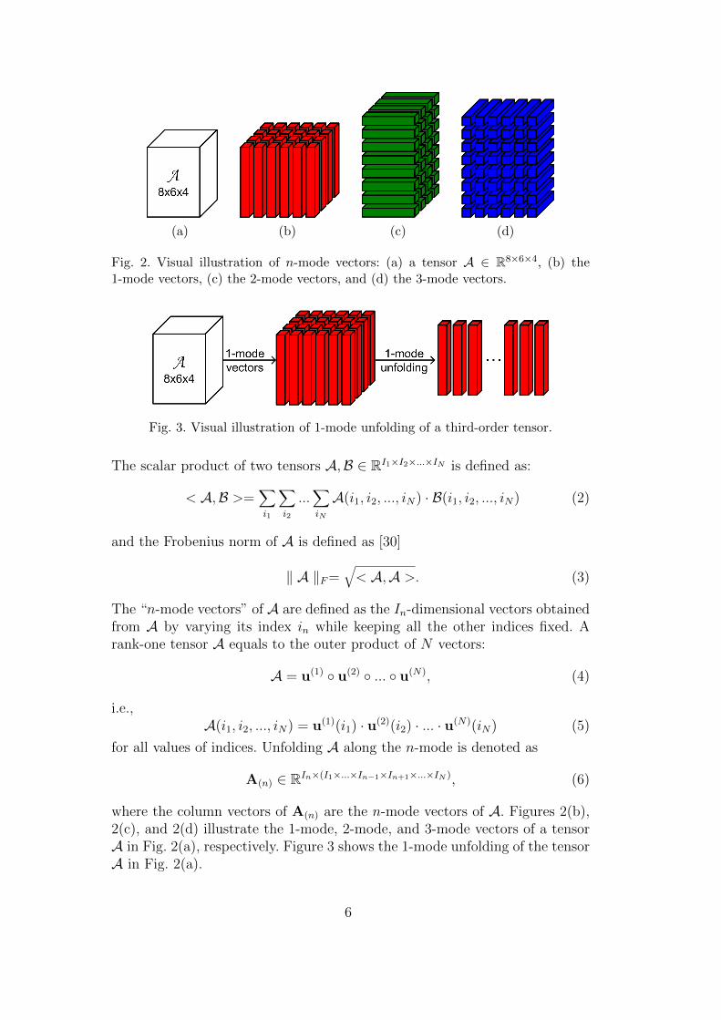
This section first reviews the notations and some basic multilinear opera-tions [30, 31, 41] that are necessary in defining the MSL problem. The im-portant concepts of multilinear projections are then introduced, including el-ementary multilinear projection (EMP), tensor-to-vector projection (TVP),and tensor-to-tensor projection (TTP), and their relationships are explored.Table 2 summarizes the important symbols used in this paper for quick refer-ence.

4

Table 2List of Important Notations

Notation Description

In the (input) dimensionality of the n-mode

M the number of training samples

N the order of a tensor object, the number of indices/modes

P the number of EMPs in a TVP

Pn the n-mode dimensionality in the projected space of a TTP

U(n) the nth projection matrix

u(n)T

p the n-mode projection of the pth EMP

vec(·) the vectorized representation

X an input tensor sample

Y the projection of X on {U(n)}

y(p) the projection of X on {u(n)T

p , n = 1, ..., N}

‖ · ‖F the Frobenius norm

2.1 Notations

This paper follows the notation conventions in multilinear algebra, patternrecognition, and adaptive learning literature [30, 31, 41]. Vectors are denotedby lowercase boldface letters, e.g., x; matrices by uppercase boldface, e.g.,X; and tensors by calligraphic letters, e.g., X . Their elements are denotedwith indices in parentheses. Indices are denoted by lowercase letters, spanningthe range from 1 to the uppercase letter of the index, e.g., p = 1, 2, ..., P . Inaddressing part of a vector/matrix/tensor, “:” denotes the full range of therespective index and n1 : n2 denotes indices ranging from n1 to n2. In thispaper, only real-valued data are considered.

2.2 Basic Multilinear Algebra

As in [30, 31, 41], an Nth-order tensor is denoted as: A ∈ RI1×I2×...×IN , whichis addressed by N indices in, n = 1, ..., N , with each in addressing the n-modeof A. The n-mode product of a tensor A by a matrix U ∈ RJn×In , denoted asA×n U, is a tensor with entries [30]:

(A×n U)(i1, ..., in−1, jn, in+1, ..., iN) =∑in

A(i1, ..., iN) ·U(jn, in). (1)

5

(a) (b) (c) (d)

Fig. 2. Visual illustration of n-mode vectors: (a) a tensor A ∈ R8×6×4, (b) the1-mode vectors, (c) the 2-mode vectors, and (d) the 3-mode vectors.

Fig. 3. Visual illustration of 1-mode unfolding of a third-order tensor.

The scalar product of two tensors A,B ∈ RI1×I2×...×IN is defined as:

< A,B >=∑i1

∑i2

...∑iN

A(i1, i2, ..., iN) · B(i1, i2, ..., iN) (2)

and the Frobenius norm of A is defined as [30]

‖ A ‖F=√< A,A >. (3)

The “n-mode vectors” of A are defined as the In-dimensional vectors obtainedfrom A by varying its index in while keeping all the other indices fixed. Arank-one tensor A equals to the outer product of N vectors:

A = u(1) ◦ u(2) ◦ ... ◦ u(N), (4)

i.e.,A(i1, i2, ..., iN) = u(1)(i1) · u(2)(i2) · ... · u(N)(iN) (5)

for all values of indices. Unfolding A along the n-mode is denoted as

A(n) ∈ RIn×(I1×...×In−1×In+1×...×IN ), (6)

where the column vectors of A(n) are the n-mode vectors of A. Figures 2(b),2(c), and 2(d) illustrate the 1-mode, 2-mode, and 3-mode vectors of a tensorA in Fig. 2(a), respectively. Figure 3 shows the 1-mode unfolding of the tensorA in Fig. 2(a).

6

The distance between tensors A and B can be measured by the Frobeniusnorm [2]:

dist(A,B) =‖ A − B ‖F . (7)

Although this is a tensor-based measure, it is equivalent to a distance measureof corresponding vector representations, as proven in [42]. Let vec(A) be thevector representation (vectorization) of A, then

dist(A,B) =‖ vec(A)− vec(B) ‖2 . (8)

This implies that the distance between two tensors as defined in (7) equals tothe Euclidean distance between their vectorized representations.

2.3 Multilinear Projections

A multilinear subspace is defined through a multilinear projection that mapsthe input tensor data from one space to another (lower-dimensional) space [43].Therefore, multilinear projection is a key concept in MSL. There are threebasic multilinear projections based on the input and output of a projection:the traditional vector-to-vector projection (VVP), TTP, and TVP.

2.3.1 Vector-to-Vector Projection

Linear projection is a standard transformation used widely in various appli-cations [44, 45]. A linear projection takes a vector x ∈ RI and projects it toanother vector y ∈ RP using a projection matrix U ∈ RI×P :

y = UTx = x×1 UT . (9)

In typical pattern recognition applications, P << I. Therefore, linear projec-tion is a VVP. When the input to VVP is an Nth-order tensor X with N > 1,it needs to be reshaped into a vector as x = vec(X ) before projection. Figure4(a) illustrates the VVP of a tensor object A. Besides the traditional linearprojection, there are alternative ways to project a tensor to a low-dimensionalspace, as shown in Fig. 4(b), which will be discussed below.

2.3.2 Tensor-to-Tensor Projection

A tensor can be projected to another tensor of the same order, named asTTP. As an Nth-order tensor X resides in the tensor space RI1

⊗RI2 ...⊗RIN

[30,43], the tensor space can be viewed as the Kronecker product of N vector(linear) spaces RI1 , RI2 , ..., RIN [43]. To project a tensor X in a tensor spaceRI1

⊗RI2 ...⊗RIN to another tensor Y in a lower-dimensional tensor space

7

RP1⊗RP2 ...

⊗RPN , where Pn ≤ In for all n, N projection matrices {U(n) ∈RIn×Pn , n = 1, ..., N} are used so that [31]

Y = X ×1 U(1)T ×2 U(2)T ...×N U(N)T . (10)

It can be done in N steps, where in the nth step, each n-mode vector isprojected to a lower dimension Pn by U(n), as shown in Fig. 5(a). Figure 5(b)demonstrates how to project a tensor in 1-mode using a 1-mode projectionmatrix, which projects each 1-mode vector of the original tensor to a low-dimensional vector.

2.3.3 Tensor-to-Vector Projection

The third multilinear projection is TVP, which is referred to as the rank-oneprojections in some works [46–48]. It projects a tensor to a vector, which canbe viewed as multiple projections from a tensor to a scalar, as illustrated inFig. 6(a), where the TVP of a tensor A ∈ R8×6×4 to a P × 1 vector consistsof P projections from A to a scalar. Thus, the projection from a tensor to a

(a) Vector-to-vector (linear) projection.

(b) Alternative ways to project a tensor.

Fig. 4. Ways to project a tensor to a low-dimensional space.

8

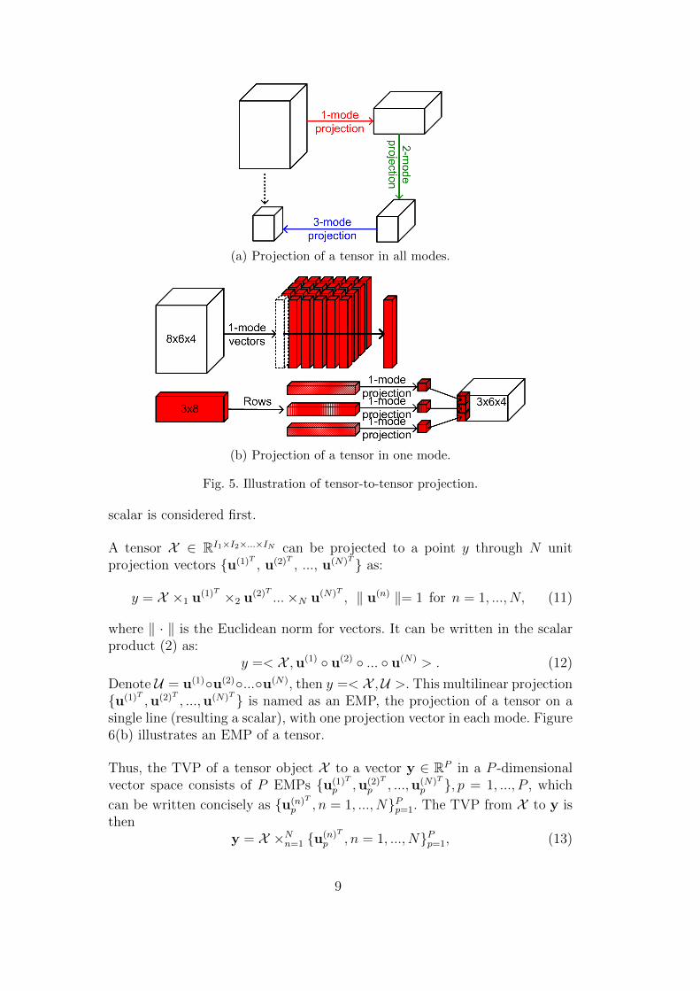
(a) Projection of a tensor in all modes.

(b) Projection of a tensor in one mode.

Fig. 5. Illustration of tensor-to-tensor projection.

scalar is considered first.

A tensor X ∈ RI1×I2×...×IN can be projected to a point y through N unitprojection vectors {u(1)T , u(2)T , ..., u(N)T } as:

y = X ×1 u(1)T ×2 u(2)T ...×N u(N)T , ‖ u(n) ‖= 1 for n = 1, ..., N, (11)

where ‖ · ‖ is the Euclidean norm for vectors. It can be written in the scalarproduct (2) as:

y =< X ,u(1) ◦ u(2) ◦ ... ◦ u(N) > . (12)

Denote U = u(1)◦u(2)◦...◦u(N), then y =< X ,U >. This multilinear projection{u(1)T ,u(2)T , ...,u(N)T } is named as an EMP, the projection of a tensor on asingle line (resulting a scalar), with one projection vector in each mode. Figure6(b) illustrates an EMP of a tensor.

Thus, the TVP of a tensor object X to a vector y ∈ RP in a P -dimensionalvector space consists of P EMPs {u(1)T

p ,u(2)T

p , ...,u(N)T

p }, p = 1, ..., P , which

can be written concisely as {u(n)T

p , n = 1, ..., N}Pp=1. The TVP from X to y isthen

y = X ×Nn=1 {u(n)T

p , n = 1, ..., N}Pp=1, (13)

9

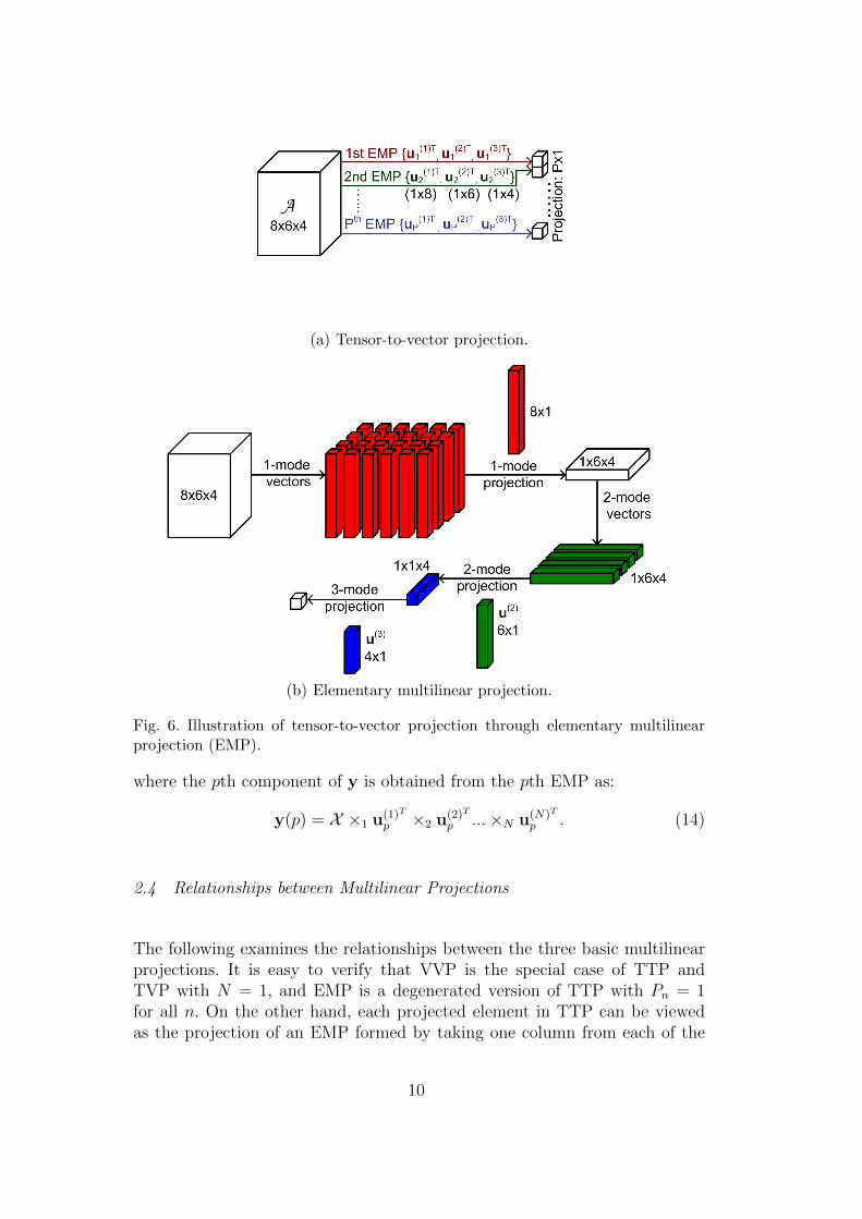
(a) Tensor-to-vector projection.

(b) Elementary multilinear projection.

Fig. 6. Illustration of tensor-to-vector projection through elementary multilinearprojection (EMP).

where the pth component of y is obtained from the pth EMP as:

y(p) = X ×1 u(1)T

p ×2 u(2)T

p ...×N u(N)T

p . (14)

2.4 Relationships between Multilinear Projections

The following examines the relationships between the three basic multilinearprojections. It is easy to verify that VVP is the special case of TTP andTVP with N = 1, and EMP is a degenerated version of TTP with Pn = 1for all n. On the other hand, each projected element in TTP can be viewedas the projection of an EMP formed by taking one column from each of the

10

projection matrices. Thus, the projected tensor in TTP is effectively obtainedthrough

∏Nn=1 Pn interdependent EMPs, while in TVP, the P EMPs obtained

sequentially are not interdependent in general.

Furthermore, the projection using an EMP {u(1)T ,u(2)T , ...,u(N)T } can be writ-ten as [28]

y =< X ,U >=< vec(X ), vec(U) >= [vec(U)]T vec(X ). (15)

Thus, an EMP is equivalent to a linear projection of vec(X ), the vectorizedrepresentation of X , on a vector vec(U). Since U = u(1) ◦ u(2) ◦ ... ◦ u(N), (15)indicates that EMP is equivalent to a linear projection with constraint on theprojection vector such that it is the vectorized representation of a rank-onetensor.

The number of parameters to be estimated in a particular projection is an im-portant concern in practice. Compared with a projection vector of size I×1 inVVP specified by I parameters (I =

∏Nn=1 In for an Nth-order tensor), an EMP

in TVP can be specified by∑N

n=1 In parameters. Hence, to project a tensor ofsize

∏Nn=1 In to a vector of size P × 1, TVP needs to estimate only P ·∑N

n=1 Inparameters, while VVP needs to estimate P · ∏N

n=1 In parameters. The im-plication in pattern recognition problem is that TVP has fewer parametersto estimate while being more constrained on the solutions, and VVP has lessconstraint on the solutions sought while having more parameters to estimate.For TTP with the same amount of dimensionality reduction

∏Nn=1 Pn = P ,∑N

n=1 Pn × In parameters need to be estimated. Table 3 contrasts the numberof parameters to be estimated by the three projections for the same amountof dimensionality reduction. From the table, it can be seen that the parame-ter estimation problem in conventional VVP becomes extremely difficult forhigher-order tensors. This often leads to the small sample size (SSS) problemin practice when there are limited number of training samples available.

Table 3Number of parameters to be estimated by three multilinear projections.

Input Output VVP TVP TTP∏Nn=1 In P P ·∏N

n=1 In P ·∑Nn=1 In

∑Nn=1 Pn × In

10× 10 4 400 80 40 (Pn = 2)

100× 100 4 40,000 800 400 (Pn = 2)

100× 100× 100 8 8,000,000 2,400 600 (Pn = 2)∏4n=1 100 16 1,600,000,000 6,400 800 (Pn = 2)

11

3 The Multilinear Subspace Learning Framework

This section formulates a general MSL framework. It defines the MSL problemin a similar way as LSL, as well as tensor and scalar scatter measures for opti-mality criterion construction. It also outlines a typical solution and discussesrelated issues.

3.1 Linear Subspace Learning

LSL algorithms [18,44] solve for a linear projection satisfying some optimalitycriteria, given a set of training samples. The problem can be formulated asfollows.

Linear Subspace Learning: A set of M vectorial samples {x1, x2, ..., xM} isavailable for learning, where each sample xm is an I×1 vector in a vector spaceRI . The LSL objective is to find a linear transformation (projection) U ∈ RI×P

such that the projected samples (the extracted features) {ym = UTxm} satisfyan optimality criterion, where ym ∈ RP×1 and P < I.

Among various LSL algorithms, principal component analysis (PCA) [19] andlinear discriminant analysis (LDA) [44] are two most widely used ones in abroad range of applications [49, 50]. PCA is an unsupervised algorithm thatdoes not require labels for the training samples, while LDA is a supervisedmethod that makes use of class specific information. Other popular LSL al-gorithms include independent component analysis (ICA) [51] and canonicalcorrelation analysis (CCA) [52].

3.2 Multilinear Subspace Learning

MSL is the multilinear extension of LSL. It solves for a multilinear projectionwith some optimality criteria, given a set of training samples. This problemcan be formulated similarly as follows.

Multilinear Subspace Learning: A set of M Nth-order tensorial samples{X1, X2, ..., XM} is available for learning, where each sample Xm is an I1×I2×...× IN tensor in a tensor space RI1×I2×...×IN . The MSL objective is to find amultilinear transformation (projection) such that the projected samples (theextracted features) satisfy an optimality criterion, where the dimensionalityof the projected space is much lower than the original tensor space.

12

Mathematically, the MSL problem can be written in a general form as

{U(n)} = arg max{U(n)}

Φ({U(n)}, {Xm}

)(16)

or{u(n)T

p }Pp=1 = arg max{u(n)T

p }Pp=1

Φ({u(n)T

p }Pp=1, {Xm}), (17)

where Φ(·) denotes a criterion function to be maximized, or without loss ofgenerality, −Φ(·) is to be minimized. {U(n)}, {u(n)T

p }Pp=1, and {Xm} are more

compact forms of {U(n), n = 1, ..., N}, {u(n)T

p , n = 1, ..., N}Pp=1, and {Xm,m =1, ...,M}, respectively.

Two key components for MSL are the multilinear projection employed and theobjective criterion to be optimized. The projection to be solved can be any ofthe three types of basic multilinear projections discussed in Sec. 2.3. Thus, thewell-studied LSL can be viewed as a special case of MSL where the projectionto be solved is a VVP. Thus, the focus of this paper will be on MSL throughTTP and TVP. This general formulation of MSL is important for evaluating,comparing, and further developing MSL solutions.

3.3 Scatter Measures for Multilinear Subspace Learning

In analogy to the definition of various scatters for vectorial features in LSL [44],tensor-based and scalar-based scatters in MSL are defined here.

Definition 1 Let {Am,m = 1, ...,M} be a set of M tensor samples in RI1⊗RI2 ...⊗RIN . The total scatter of these tensors is defined as:

ΨTA =M∑

m=1

‖ Am − A ‖2F , (18)

where A is the mean tensor calculated as

A =1

M

M∑m=1

Am. (19)

The n-mode total scatter matrix of these samples is then defined as:

S(n)TA

=M∑

m=1

(Am(n) − A(n)

) (Am(n) − A(n)

)T, (20)

where Am(n) is the n-mode unfolded matrix of Am.

Definition 2 Let {Am,m = 1, ...,M} be a set of M tensor samples in RI1⊗

13

RI2 ...⊗RIN . The between-class scatter and the within-class scatter of these

tensors are defined as:

ΨBA =C∑c=1

Mc ‖ Ac − A ‖2F , and ΨWA =M∑

m=1

‖ Am − Acm ‖2F , (21)

respectively, where C is the number of classes, Mc is the number of samplesfor class c, cm is the class label for the mth sample Am, A is the mean tensor,and the class mean tensor is

Ac =1

Mc

∑m,cm=c

Am. (22)

Next, the n-mode scatter matrices are defined accordingly.

Definition 3 The n-mode between-class scatter matrix of these samples isdefined as:

S(n)BA

=C∑c=1

Mc ·(Ac(n) − A(n)

) (Ac(n) − A(n)

)T, (23)

and the n-mode within-class scatter matrix of these samples is defined as:

S(n)WA

=M∑

m=1

(Am(n) − Acm(n)

) (Am(n) − Acm(n)

)T, (24)

where Ac(n) is the n-mode unfolded matrix of Ac.

The tensor scatters defined above are for MSL based on TTP. For MSL basedon TVP, scalar-based scatters are defined, which can be viewed as degeneratedversions of the vector-based or tensor-based scatters.

Definition 4 Let {am,m = 1, ...,M} be a set of M scalar samples. The totalscatter of these scalars is defined as:

STa =M∑

m=1

(am − a)2, (25)

where a is the mean scalar calculated as

a =1

M

M∑m=1

am. (26)

Definition 5 Let {am,m = 1, ...,M} be a set of M scalar samples. The

14

between-class scatter of these scalars is defined as:

SBa =C∑c=1

Mc(ac − a)2, (27)

and the within-class scatter of these scalars is defined as:

SWa =M∑

m=1

(am − acm)2, (28)

where

ac =1

Mc

∑m,cm=c

am. (29)

3.4 Typical Approach and Algorithmic Issues

While a linear projection (VVP) in LSL often has closed-form solutions, thisis not the case for TTP and TVP in MSL. Instead, these two tensor-basedprojections have N sets of parameters to be solved, one in each mode, andthe solution to one set often depends on the other sets (except when N = 1,the linear case), making their simultaneous estimation extremely difficult, ifnot impossible. Therefore, a suboptimal, iterative procedure originated fromthe alternating least square (ALS) algorithm [53–55] is usually employed tosolve the tensor-based projections by alternating between solving one set ofparameters (in one mode) at a time. Specifically, the parameters for eachmode are estimated in turn separately and are conditioned on the parametervalues for the other modes. At each step, by fixing the parameters in all themodes but one mode, a new objective function depending only on the modeleft free to vary is optimized and this conditional subproblem is linear andmuch simpler to solve through unfolding tensors to matrices. The parameterestimations for each mode are obtained in this way sequentially and iterativelyuntil convergence. This process is described in Fig. 7(a) and also illustratedin Fig. 7(b).

Consequently, the issues due to the iterative nature of the solution, such as ini-tialization, the order of solving the projections, termination, and convergence,need to be addressed. In addition, for MSL through TTP, a mechanism is of-ten needed to determine the desired subspace dimensionality {P1, P2, ..., PN}.This is because it is costly to exhaustively test the large number of possiblecombinations of the N values, P1, P2, ..., PN , for a specific amount of dimen-sionality reduction, especially for higher-order tensors. In contrast, the valueP is relatively easier to determine for MSL through TVP.

To end this section, Table 4 summarizes the key differences between MSL

15

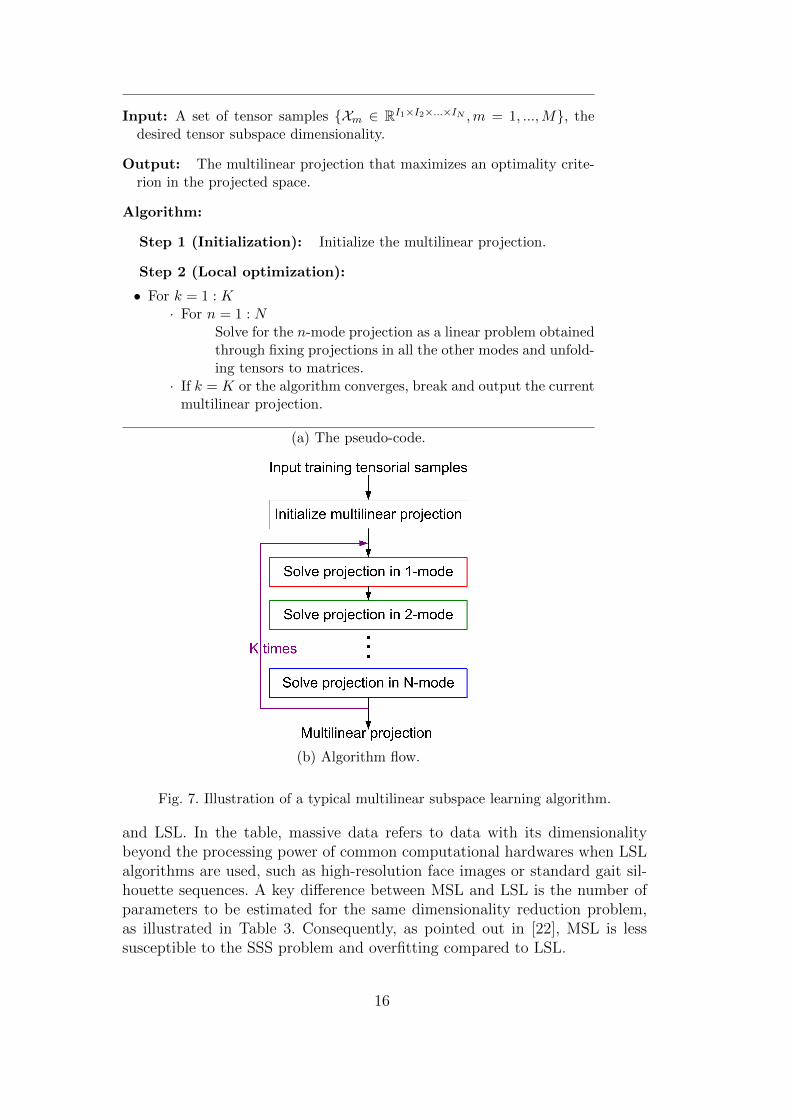
Input: A set of tensor samples {Xm ∈ RI1×I2×...×IN ,m = 1, ...,M}, thedesired tensor subspace dimensionality.

Output: The multilinear projection that maximizes an optimality crite-rion in the projected space.

Algorithm:

Step 1 (Initialization): Initialize the multilinear projection.

Step 2 (Local optimization):

• For k = 1 : K· For n = 1 : N

Solve for the n-mode projection as a linear problem obtainedthrough fixing projections in all the other modes and unfold-ing tensors to matrices.

· If k = K or the algorithm converges, break and output the currentmultilinear projection.

(a) The pseudo-code.

(b) Algorithm flow.

Fig. 7. Illustration of a typical multilinear subspace learning algorithm.

and LSL. In the table, massive data refers to data with its dimensionalitybeyond the processing power of common computational hardwares when LSLalgorithms are used, such as high-resolution face images or standard gait sil-houette sequences. A key difference between MSL and LSL is the number ofparameters to be estimated for the same dimensionality reduction problem,as illustrated in Table 3. Consequently, as pointed out in [22], MSL is lesssusceptible to the SSS problem and overfitting compared to LSL.

16

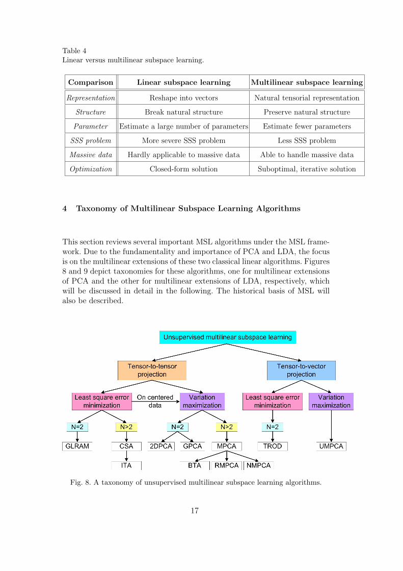
Table 4Linear versus multilinear subspace learning.

Comparison Linear subspace learning Multilinear subspace learning

Representation Reshape into vectors Natural tensorial representation

Structure Break natural structure Preserve natural structure

Parameter Estimate a large number of parameters Estimate fewer parameters

SSS problem More severe SSS problem Less SSS problem

Massive data Hardly applicable to massive data Able to handle massive data

Optimization Closed-form solution Suboptimal, iterative solution

4 Taxonomy of Multilinear Subspace Learning Algorithms

This section reviews several important MSL algorithms under the MSL frame-work. Due to the fundamentality and importance of PCA and LDA, the focusis on the multilinear extensions of these two classical linear algorithms. Figures8 and 9 depict taxonomies for these algorithms, one for multilinear extensionsof PCA and the other for multilinear extensions of LDA, respectively, whichwill be discussed in detail in the following. The historical basis of MSL willalso be described.

Fig. 8. A taxonomy of unsupervised multilinear subspace learning algorithms.

17

4.1 Unsupervised Multilinear Subspace Learning Algorithms

The development of unsupervised MSL started with the treatment of imagesdirectly as matrices rather than vectors.

4.1.1 Unsupervised MSL through TTP

A two-dimensional PCA (2DPCA) algorithm is proposed in [56]. This al-gorithm solves for a linear transformation that projects an image to a low-dimensional matrix while maximizing the variance measure. It works directlyon image matrices but there is only one linear transformation in the 2-mode.Thus, the image data is projected in the 2-mode (the row mode) only whilethe projection in the 1-mode (the column mode) is ignored, resulting in poordimensionality reduction. The projection can be viewed as a special case ofsecond-order TTP, where the 1-mode projection matrix is an identity matrix.

A more general algorithm named the generalized low rank approximation ofmatrices (GLRAM) was introduced in [57], which takes into account the spa-tial correlation of the image pixels within a localized neighborhood and appliestwo linear transforms to both the left and right sides of input image matrices.This algorithm solves for two linear transformations that project an image toa low-dimensional matrix while minimizing the least-square (reconstruction)error measure. Thus, projections in both modes are involved and the projec-tion is TTP with N = 2. Better dimensionality reduction results than [56] areobtained according to [57].

Although GLRAM exploits both modes for subspace learning, it is formulatedfor matrices only. Later, the work in [58] presents tensor approximation meth-ods for third-order tensors using slice projection, while the so-called concur-

Fig. 9. A taxonomy of supervised multilinear subspace learning algorithms.

18

rent subspaces analysis (CSA) is formulated in [27] for general tensor objectsas a generalization of GLRAM for higher-order tensors. The CSA algorithmsolves for a TTP minimizing a reconstruction error metric, however, how todetermine the tensor subspace dimensionality is not addressed in this work.

Whereas GLRAM and CSA advanced unsupervised MSL, they are both for-mulated with the objective of optimal reconstruction or approximation of ten-sors. Therefore, they ignored an important centering step in unsupervisedsubspace learning algorithms developed for recognition, such as the classicalPCA, where the data is centered first before obtaining the subspace projec-tion. It should be pointed out that for the reconstruction or approximationproblem, centering is not essential, as the (sample) mean is the main focusof attention [21]. However, in recognition applications where the solutions in-volve eigenproblems, non-centering (in other words, an average different fromzero) can potentially affect the eigen-decomposition in each mode and lead toa solution that captures the variation with respect to the origin rather thancapturing the true variation of the data (with respect to the data center) [21].

In contrast, the generalized PCA (GPCA) proposed in [1] is an extension ofPCA that works on matrices. GPCA is exactly the same as GLRAM exceptthat the projection takes the centered data rather than the original coordinateas input. Nonetheless, this work is formulated only for matrices, and importantissues such as initialization and subspace dimensionality determination are notstudied in this work either.

The multilinear PCA (MPCA) algorithm proposed in [21] generalizes GPCAto work for tensors of any order, where the objective is to find a TTP thatcaptures most of the original tensorial input variations (Definition 1). Fur-thermore, methods for systematic subspace dimensionality determination areproposed for the first time in the literature, in contrast to heuristic methodsin [27, 57]. With the introduction of a discriminative tensor feature selectionmechanism, MPCA is further combined with LDA for general tensor objectrecognition in [21].

In [59], a TTP-based MSL algorithm named Bayesian tensor analysis (BTA)is proposed to generalize the Bayesian PCA algorithm [60] and develop prob-abilistic graphical models for tensors. BTA is able to determine the subspacedimensionality automatically by setting a series of hyper parameters. As themean is subtracted from the input tensor in dimensionality reduction usingBTA, it can be considered as a probabilistic extension of MPCA as well. In [61],two robust MPCA (RMPCA) algorithms are proposed, where iterative algo-rithms are derived on the basis of Lagrange multipliers to deal with sampleoutliers and intra-sample outliers. In [62], the non-negative MPCA (NMPCA)extends MPCA to constrain the projection matrices to be non-negative. Fur-thermore, NMPCA preserves the non-negativity of the original tensor samples,

19

which is important when the underlying data factors have physical or psycho-logical interpretation. The solution for NMPCA is developed by exploiting thestructure of the Grassmann manifold [62].

In addition, an incremental tensor analysis (ITA) framework is proposed in [17]for summarizing higher-order data streams represented as tensors. The datasummary is obtained through TTP and is updated incrementally. Three vari-ants of ITA are introduced in [17]: dynamic tensor analysis (DTA) that in-crementally maintains covariance matrices for all modes and uses the leadingeigenvectors of covariance matrices as projection matrices [15], streaming ten-sor analysis (STA) that directly updates the leading eigenvectors of covariancematrices using the SPIRIT algorithm [63], and window-based tensor analysis(WTA) that uses similar updates as DTA while performing alternating iter-ation to further improve the results. The ITA framework focuses on approxi-mation problem, hence, the objective is to minimize the least square error andit can be considered as an incremental version of CSA for streaming data.

4.1.2 Unsupervised MSL through TVP

In comparison to the review above, there are much fewer unsupervised MSLalgorithms based on TVP. The tensor rank-one decomposition (TROD) al-gorithm introduced in [64] is TVP-based and it is formulated only for imagematrices. This algorithm looks for a second-order TVP that projects an imageto a low-dimensional vector while minimizing a least-square (reconstruction)error measure. Hence, the input data is not centered before learning. The solu-tion of TROD relies on a heuristic procedure of successive residue calculation,i.e., after obtaining the pth EMP, the input image is replaced by its residue.

None of the above unsupervised MSL algorithms takes into account the cor-relations among features and shares an important property with PCA, i.e.,zero-correlation among extracted features. It is well-known that PCA derivesuncorrelated features, which contain minimum redundancy and ensure linearindependence among features. Uncorrelated features can also greatly simplifythe subsequent classification task and they are highly desirable in recogni-tion applications. An uncorrelated MPCA (UMPCA) algorithm is proposedin [25], which extracts uncorrelated multilinear features through TVP whilecapturing most of the variation in the original data input (Definition 4). TheUMPCA solution consists of sequential iterative steps for successive variancemaximization. The work in [25] has also derived a systematic way to deter-mine the maximum number of uncorrelated multilinear features that can beextracted by the method.

20

4.2 Supervised Multilinear Subspace Learning Algorithms

Similar to unsupervised MSL, the development of supervised MSL startedwith 2D extensions of LDA.

4.2.1 Supervised MSL through TTP

Like GLRAM and GPCA, the 2D LDA (2DLDA) introduced in [65] solvesfor two linear transformations that project an image to a low-dimensionalmatrix, but with a different objective criterion. For the input image samples,the between-class and within-class scatter measures are defined for matrixrepresentations (Definition 2). A matrix-based discrimination criterion is thendefined as the scatter ratio, which is to be maximized in 2DLDA. Unlike theunsupervised MSL algorithms reviewed above, 2DLDA does not converge overiterations.

Later, as a higher-order extension of 2DLDA, the discriminant analysis withtensor representation (DATER) 1 was proposed to perform discriminant anal-ysis on more general tensorial inputs [2]. The DATER algorithm solves for aTTP maximizing the tensor-based scatter ratio (Definition 2). However, thisalgorithm does not converge over iterations either.

In [23], the general tensor discriminant analysis (GTDA) algorithm is pro-posed. The GTDA algorithm also solves for a TTP. The difference with DATERis that it maximizes a tensor-based scatter difference criterion (Definition 2),with a tuning parameter involved [66]. The criterion used is dependent onthe coordinate system, as pointed out in [67], and the tuning parameter isheuristically determined in [23]. In contrast with 2DLDA/DATER, this al-gorithm has good convergence property [23] and it is the first discriminativeMSL algorithm that converges to a local solution.

4.2.2 Supervised MSL through TVP

In this category, the first algorithm is the tensor rank-one discriminant analysis(TR1DA) algorithm proposed in [46, 47], derived from the TROD algorithm[64]. The TR1DA algorithm is formulated for general tensor objects and itlooks for a TVP that projects a tensor to a low-dimensional vector whilemaximizing the scalar scatter difference criterion (Definition 5). Therefore, thecriterion is also dependent on the coordinate system and there is no way todetermine the optimal tuning parameter either. Furthermore, as in TROD, this

1 Here, the name used when the algorithm was first proposed is adopted as it ismore commonly referred to in the literature.

21

algorithm also relies on the repeatedly-calculated residues, originally proposedin [68] for tensor approximation. The adoption of this heuristic procedure herelacks theoretical explanation for a discriminative criterion.

Similar to the case of unsupervised MSL, the supervised MSL algorithms dis-cussed so far do not take the correlations among features into account andthey do not derive uncorrelated features as in the classical LDA [69, 70]. Asmentioned in Sec. 4.1.2, uncorrelated features are highly desirable in many ap-plications [70]. An uncorrelated multilinear discriminant analysis (UMLDA)algorithm is formulated in [26]. UMLDA aims to extract uncorrelated dis-criminative features directly from tensorial data through solving a TVP tomaximize a scalar scatter ratio criterion (Definition 5). The solution consistsof sequential iterative processes and incorporates an adaptive regularizationprocedure to enhance the performance in the small sample size scenario. Fur-thermore, an aggregation scheme is adopted to combine differently initializedand regularized UMLDA recognizers for enhanced generalization performancewhile alleviating the regularization parameter selection problem. This exten-sion is called regularized UMLDA with aggregation (R-UMLDA-A) [26].

4.3 The Historical Basis of MSL

Multilinear algebra, the extension of linear algebra, has been studied in math-ematics around the middle of the 20th century [29]. It built on the concept oftensors and developed the theory of tensor spaces.

A popular early application of multilinear algebra is multi-way analysis inpsychometrics and chemometrics starting from the 60s and 70s, for factoranalysis of multi-way data sets, which are higher-order tensors characterized byseveral sets of categorical variables that are measured in a crossed fashion [53–55,71]. Two main types of decomposition methods have been developed in thisfield: the Tucker decomposition [30,41,71,72], and the canonical decomposition(CANDECOMP) [30, 41, 53], also known as the parallel factors (PARAFAC)decomposition [30,41,54]. There are also other tensor decompositions such asCANDECOMP with linear constraints (CANDELINC) [73].

In the 90s, the developments in higher-order statistics of multivariate stochas-tic variables have attracted interests in higher-order tensors from the signalprocessing community [74]. The Tucker decomposition was reintroduced andfurther developed in [30] as an extension of the singular value decomposition(SVD) to higher-order tensors: the higher-order SVD (HOSVD) solution. Itscomputation leads to the calculation of N different matrix SVDs of differentlyunfolded matrices. The ALS algorithm for the best Rank-(R1, R2, ..., RN) ap-proximation of higher-order tensors was studied in [31], where tensor data was

22

iteratively projected into a lower dimensional tensor space. The applicationof HOSVD truncation and the best Rank-(R1, R2, ..., RN) approximation todimensionality reduction in ICA was discussed in [75].

The work in [30,31] led to the development of new multilinear algorithms andthe exploration of new application areas for tensor data analysis. Multilinearanalysis of image data is pioneered by the TensorFace method [76, 77], whichemploys the multilinear algorithms proposed in [30,31] to analyze the factorsinvolved in the formation of facial images. Similar analysis has also been donefor motion signatures [78] and gait sequences [79]. However, in these multiplefactor analysis work, input data such as images or video sequences are stillrepresented as vectors. These vectors are arranged into a tensor accordingto multiple factors involved in their formation for subsequent analysis. Suchtensor formation needs a large number of training samples captured undervarious conditions, which is often impractical and may have the missing-dataproblem. Furthermore, the tensor data size is usually huge, leading to highmemory and computational demands.

In the last few years, several methods were proposed for direct learning of asubspace from tensorial data [1,2,21,23,25–27,47,56,64,65]. Besides the MSLalgorithms reviewed above, there is also a multilinear extension of the CCAalgorithm named as tensor CCA in [80]. In addition, solutions are proposedin [81, 82] to rearrange elements within a tensor to maximize the correlationsamong n-mode vectors for better dimensionality reduction performance. Fur-thermore, systematic treatment of this topic has appeared in [28,42]. Besidesthe multilinear extensions of LSL algorithms, multilinear extensions of lin-ear graph-embedding algorithms were also introduced in [43, 48, 83–86], in asimilar fashion as the existing MSL algorithms reviewed in this paper.

5 Multilinear Subspace Learning Applications

Due to the advances in sensor and storage technology, MSL is becoming in-creasingly popular in a wide range of application domains involving tensor-structured data sets. This section will summarize several applications of MSLalgorithms in real-world applications, including face recognition and gait recog-nition in biometrics, music genre classification in audio signal processing, EEGsignal classification in biomedical engineering, anomaly detection in data min-ing, and visual content analysis in computer vision. Other MSL applicationsinclude handwritten digit recognition [27, 57], image compression [1, 27, 64],image/video retrieval [1, 87], and object categorization and recognition [46].For more general tensor data applications, [35], [88], [89] and [90] are goodreferences.

23

5.1 Face Recognition and Gait Recognition

Face and gait are two typical physiological and behavioral biometrics, respec-tively. Compared with other biometric traits, face and gait have the uniqueproperty that they facilitate human recognition at a distance, which is ex-tremely important in surveillance applications. Face recognition has a largenumber of commercial security and forensic applications, including video surveil-lance, access control, mugshot identification, and video communications [10,91]. Gait is a person’s walking style and it is a complex spatio-temporal bio-metric [10, 91]. The interest in gait recognition is strongly motivated by theneed for an automated human identification system at a distance in visualsurveillance and monitoring applications in security-sensitive environments,e.g., banks, parking lots, malls, and transportation hubs such as airports andtrain stations [21]. Many MSL algorithms are first applied to appearance-based learning for face recognition [2, 27, 56, 57, 86, 92, 93] and/or gait recog-nition [21, 23, 94–97], where the input face images or binary gait silhouettesequences are treated as tensorial holistic patterns as shown in Fig. 1.

5.2 Music Genre Classification

Music genre is a popular description of music content for music databaseorganization. The NMPCA algorithm proposed in [62] is designed for musicgenre classification, combined with the nearest neighbor or support vectormachines (SVM) classifiers. A 2D joint acoustic and modulation frequencyrepresentation of music signals is utilized in this work to capture slow temporalmodulations [62], inspired by psychophysiological investigations on the humanauditory system. The acoustic signal is first converted to a time-frequencyauditory spectrogram and a wavelet transform is applied to each row of thisspectrogram to estimate its temporal modulation content through modulationscale analysis [62]. In three different sets of experiments on public music genredata sets, NMPCA has achieved the state-of-the-art classification results.

5.3 EEG Signal Classification

Electroencephalography (EEG) records brain activities as multichannel timeseries from multiple electrodes placed on the scalp of a subject to provide adirect communication channel between brain and computer, and it is widelyused in noninvasive brain computer interfaces (BCI) applications [98]. In [5], atensor-based EEG classification scheme is proposed, where the wavelet trans-form is applied to EEG signals to result in third-order tensor representations

24

in the spatial-spectral-temporal domain. GTDA is then applied to obtain low-dimensional tensors, from which discriminative features are selected for SVMclassification. Motor imagery experiments on three data sets demonstrate thatthe proposed scheme can outperform many other existing EEG signal classifi-cation schemes, especially when there is no prior neurophysiologic knowledgeavailable for EEG signal preprocessing.

5.4 Anomaly Detection

In streaming data applications such as network forensics, large volumes ofhigh-order data continuously arrive incrementally. It is challenging to per-form incremental pattern discovery on such data streams. The ITA frame-work in [17] is devised to tackle this problem and anomaly detection is oneof its targeted applications. The abnormality is modeled by the reconstruc-tion error of incoming tensor data streams and a large reconstruction erroroften indicates an anomaly. The proposed method is illustrated on a networkmonitoring example, where three types of anomalies (abnormal source hosts,abnormal destination hosts, and abnormal ports) can be detected with veryhigh precision.

5.5 Visual Content Analysis

As a dimensionality reduction technique, MSL can also be used for variousvisual content analysis tasks [87, 99–103]. E.g., the MPCA algorithm is usedto visualize and summarize a crowd video sequence in a 2D subspace in [100].In [101], an optical flow tensor is built and GTDA is used to reduce thedimensionality for further semantic analysis of video sequences. For 3D facialdata modeling, the BTA algorithm is employed for the 3D facial expressionretargeting task [59]. In [102], a modified version of the DTA algorithm (withmean and variance updating) is applied on a weighted tensor representationfor visual tracking of human faces, and in [103], an automatic human ageestimation method is developed using MPCA for dimensionality reduction oftensorial Gaussian receptive maps.

6 Conclusions and Future Works

This paper presents a survey of an emerging dimensionality reduction ap-proach for direct feature extraction from tensor data: multilinear subspacelearning. It reduces the dimensionality of massive data directly from their

25

natural multidimensional representation: tensors. This survey covers multi-linear projections, MSL framework, typical MSL solutions, MSL taxonomies,and MSL applications. MSL is a new field with many open issues to be ex-amined further. The rest of this section outlines several research topics thatworth further investigation. Two main directions have been identified. One istowards the development of new MSL solutions, while the other is towards theexploration of new MSL applications.

In future research, new algorithms can be investigated along the followingdirections. The systematic treatment on MSL will benefit the development ofnew multilinear learning algorithms, especially by extending the rich ideas andalgorithms in the linear counterparts to the multilinear case. This paper hasfocused on the extensions of PCA and LDA to their multilinear counterparts.In future work, more complex multilinear mapping can be investigated, forexample, by developing multilinear extensions of graph-embedding algorithmssuch as Isomap [104], Locally Linear Embedding [105], and Locality PreservingProjections [106,107] under the MSL framework. As mentioned in Section 4.3,there have been some developments already in this area [43, 48, 84–86]. TheMSL framework can help the understanding of these existing solutions andit can also benefit their further development. Furthermore, in MSL, there arestill many open problems remaining, such as the optimal initialization, theoptimal projection order, and the optimal stopping criterion. There has beensome attempts in solving some of these problems in [21]. However, furtherresearch in this direction is needed for deeper understanding on these issuesand even alternative optimization strategies can be explored.

Besides the applications reviewed in Sec. 5, there are a wide range of appli-cations dealing with real-world tensor objects where MSL may be useful, asmentioned in the Introduction of this paper. Examples include high-resolutionand 3D face detection and recognition [108–111], clustering or retrieval of im-ages or 3D objects [8,112], space-time analysis of video sequences [11,113], andspace-time super-resolution [14]. In addition, massive streaming data are fre-quently organized as multidimensional objects, such as those in social networkanalysis, web data mining, and sensor network analysis [17]. Some tensor-basedtechniques have been developed in these fields [15,16] and further investigationof MSL for these applications under the framework presented in this paper canbe fruitful.

To summarize, the recent prevalence of applications involving massive mul-tidimensional data has increased the demand for technical developments inthe emerging research field of MSL. This overview provides a foundation uponwhich solutions for many interesting and challenging problems in tensor dataapplications can be built. It is the authors’ hope that this unifying review andthe insights provided in this paper will foster more principled and successfulapplications of MSL in a wide range of research disciplines.

26

Acknowledgment

The authors would like to thank the anonymous reviewers for their insightfulcomments, which have helped to improve the quality of this paper.

References

[1] J. Ye, R. Janardan, Q. Li, GPCA: An efficient dimension reduction scheme forimage compression and retrieval, in: The Tenth ACM SIGKDD Int. Conf. onKnowledge Discovery and Data Mining, 2004, pp. 354–363.

[2] S. Yan, D. Xu, Q. Yang, L. Zhang, X. Tang, H. Zhang, Multilinear discriminantanalysis for face recognition, IEEE Transactions on Image Processing 16 (1)(2007) 212–220.

[3] J. Lu, K. N. Plataniotis, A. N. Venetsanopoulos, Face recognition usingkernel direct discriminant analysis algorithms, IEEE Transactions on NeuralNetworks 14 (1) (2003) 117–126.

[4] H. Lu, J. Wang, K. N. Plataniotis, A review on face and gait recognition:System, data and algorithms, in: S. Stergiopoulos (Ed.), Advanced SignalProcessing Handbook, 2nd Edition, CRC Press, Boca Raton, Florida, 2009,pp. 303–330.

[5] J. Li, L. Zhang, D. Tao, H. Sun, Q. Zhao, A prior neurophysiologic knowledgefree tensor-based scheme for single trial eeg classification, IEEE Transactionson Neural Systems and Rehabilitation Engineering 17 (2) (2009) 107–115.

[6] H. Lu, K. N. Plataniotis, A. N. Venetsanopoulos, Regularized common spatialpatterns with generic learning for EEG signal classification, in: Proc. 31st Int.Conf. of the IEEE Engineering in Medicine and Biology Society, 2009.

[7] J. Ye, T. Li, T. Xiong, R. Janardan, Using uncorrelated discriminant analysisfor tissue classification with gene expression data, IEEE/ACM Trans. Comput.Biology Bioinformatics 1 (4) (2004) 181–190.

[8] H. S. Sahambi, K. Khorasani, A neural-network appearance-based 3-D objectrecognition using independent component analysis, IEEE Transactions onNeural Networks 14 (1) (2003) 138–149.

[9] N. Renard, S. Bourennane, Dimensionality reduction based on tensor modelingfor classification methods, IEEE Transactions on Geoscience and RemoteSensing 47 (4) (2009) 1123–1131.

[10] R. Chellappa, A. Roy-Chowdhury, S. Zhou, Recognition of Humans and TheirActivities Using Video, Morgan & Claypool Publishers, San Rafael, California,2005.

27

[11] R. D. Green, L. Guan, Quantifying and recognizing human movement patternsfrom monocular video images-part II: applications to biometrics, IEEETransactions on Circuits and Systems for Video Technology 14 (2) (2004)191–198.

[12] D. R. Hardoon, J. Shawe-Taylor, Decomposing the tensor kernel support vectormachine for neuroscience data with structure labels, Machine Learning 79 (1-2)(2010) 29–46.

[13] X. He, Incremental semi-supervised subspace learning for image retrieval, in:ACM conference on Multimedia 2004, 2004, pp. 2–8.

[14] E. Shechtman, Y. Caspi, M. Irani, Space-time super-resolution, IEEETransactions on Pattern Analysis and Machine Intelligence 27 (4) (2005) 531–545.

[15] J. Sun, D. Tao, C. Faloutsos, Beyond streams and graphs: dynamic tensoranalysis, in: Proc. the 12th ACM SIGKDD int. conf. on Knowledge discoveryand data mining, 2006, pp. 374–383.

[16] J. Sun, Y. Xie, H. Zhang, C. Faloutsos, Less is more: Sparse graph miningwith compact matrix decomposition, Statistical Analysis and Data Mining1 (1) (2008) 6–22.

[17] J. Sun, D. Tao, S. Papadimitriou, P. S. Yu, C. Faloutsos, Incremental tensoranalysis: Theory and applications, ACM Trans. on Knowledge Discovery fromData 2 (3) (2008) 11:1–11:37.

[18] G. Shakhnarovich, B. Moghaddam, Face recognition in subspaces, in: S. Z. Li,A. K. Jain (Eds.), Handbook of Face Recognition, Springer-Verlag, 2004, pp.141–168.

[19] I. T. Jolliffe, Principal Component Analysis, 2nd Edition, Springer Serires inStatistics, 2002.

[20] S. Z. Li, A. K. Jain, Introduction, in: S. Z. Li, A. K. Jain (Eds.), Handbookof Face Recognition, Springer-Verlag, 2004, pp. 1–11.

[21] H. Lu, K. N. Plataniotis, A. N. Venetsanopoulos, MPCA: Multilinear principalcomponent analysis of tensor objects, IEEE Transactions on Neural Networks19 (1) (2008) 18–39.

[22] D. Tao, X. Li, X. Wu, W. Hu, S. J. Maybank, Supervised tensor learning,Knowledge and Information Systems 13 (1) (2007) 1–42.

[23] D. Tao, X. Li, X. Wu, S. J. Maybank, General tensor discriminant analysisand gabor features for gait recognition, IEEE Transactions on Pattern Analysisand Machine Intelligence 29 (10) (2007) 1700–1715.

[24] D. Tao, X. Li, X. Wu, S. J. Maybank, Tensor rank one discriminantanalysisa convergent method for discriminative multilinear subspace selection,Neurocomputing 71 (10-12) (2008) 1866–1882.

28

[25] H. Lu, K. N. Plataniotis, A. N. Venetsanopoulos, Uncorrelated multilinearprincipal component analysis for unsupervised multilinear subspace learning,IEEE Transactions on Neural Networks 20 (11) (2009) 1820–1836.

[26] H. Lu, K. N. Plataniotis, A. N. Venetsanopoulos, Uncorrelated multilineardiscriminant analysis with regularization and aggregation for tensor objectrecognition, IEEE Transactions on Neural Networks 20 (1) (2009) 103–123.

[27] D. Xu, S. Yan, L. Zhang, S. Lin, H.-J. Zhang, T. S. Huang, Reconstruction andrecognition of tensor-based objects with concurrent subspaces analysis, IEEETransactions on Circuits and Systems for Video Technology 18 (1) (2008) 36–47.

[28] H. Lu, K. N. Plataniotis, A. N. Venetsanopoulos, A taxonomy of emergingmultilinear discriminant analysis solutions for biometric signal recognition,in: N. V. Boulgouris, K. Plataniotis, E. Micheli-Tzanakou (Eds.), Biometrics:Theory, Methods, and Applications, Wiley/IEEE, 2009, pp. 21–45.

[29] W. H. Greub, Multilinear Algebra, Springer-Verlag, Berlin, 1967.

[30] L. D. Lathauwer, B. D. Moor, J. Vandewalle, A multilinear singualr valuedecomposition, SIAM Journal of Matrix Analysis and Applications 21 (4)(2000) 1253–1278.

[31] L. D. Lathauwer, B. D. Moor, J. Vandewalle, On the best rank-1 andrank-(R1, R2, ..., RN ) approximation of higher-order tensors, SIAM Journal ofMatrix Analysis and Applications 21 (4) (2000) 1324–1342.

[32] L. Qi, W. Sun, Y. Wang, Numerical multilinear algebra and its applications,FRONTIERS OF MATHEMATICS IN CHINA 2 (4) (2007) 501–526.

[33] D. Muti, S. Bourennane, Survey on tensor signal algebraic filtering, SignalProcessing 87 (2) (2007) 237–249.

[34] E. Acar, B. Yener, Unsupervised multiway data analysis: A literature survey,IEEE Transactions on Knowledge and Data Engineering 21 (1) (2009) 6–20.

[35] T. G. Kolda, B. W. Bader, Tensor decompositions and applications, SIAMReview 51 (3) (2009) 455–500.

[36] S. Zafeiriou, Algorithms for nonnegative tensor factorization, in: S. Aja-Fernandez, R. d. L. Garcıa, D. Tao, X. Li (Eds.), Tensors in Image Processingand Computer Vision, Springer, 2009, pp. 105–124.

[37] T. Hazan, S. Polak, A. Shashua, Sparse image coding using a 3D non-negativetensor factorization, in: Proc. IEEE Conference on Computer Vision, Vol. 1,2005, pp. 50–57.

[38] A. Shashua, T. Hazan, Non-negative tensor factorization with applications tostatistics and computer vision, in: Proc. Int. Conf. on Machine Learning, 2005,pp. 792–799.

29

[39] R. Bro, Multi-way analysis in the food industry - models, algorithms andapplications, Ph.D. thesis, University of Amsterdam, The Netherlands (1998).URL http://www.models.kvl.dk/sites/default/files/brothesis_0.pdf

[40] A. K. Smilde, R. Bro, P. Geladi, Multi-way Analysis, John Wiley and Sons,2004.

[41] B. W. Bader, T. G. Kolda, Algorithm 862: Matlab tensor classes for fastalgorithm prototyping, ACM Trans. on Mathematical Software 32 (4) (2006)635–653.

[42] H. Lu, Multilinear subspace learning for face and gait recognition, Ph.D. thesis,University of Toronto (2008).URL https://tspace.library.utoronto.ca/handle/1807/16750

[43] X. He, D. Cai, P. Niyogi, Tensor subspace analysis, in: Advances in NeuralInformation Processing Systems 18 (NIPS), 2005.

[44] R. O. Duda, P. E. Hart, D. G. Stork, Pattern Classification, 2nd Edition, WileyInterscience, 2001.

[45] T. K. Moon, W. C. Stirling, Mathematical methods and Algorithms for SignalProcessing, Prentice Hall, 2000.

[46] Y. Wang, S. Gong, Tensor discriminant analysis for view-based objectrecognition, in: Proc. Int. Conf. on Pattern Recognition, Vol. 3, 2006, pp.33–36.

[47] D. Tao, X. Li, X. Wu, S. J. Maybank, Elapsed time in human gait recognition:A new approach, in: Proc. IEEE Int. Conf. on Acoustics, Speech and SignalProcessing, Vol. 2, 2006, pp. 177–180.

[48] G. Hua, P. A. Viola, S. M. Drucker, Face recognition using discriminativelytrained orthogonal rank one tensor projections, in: Proc. IEEE Conference onComputer Vision and Pattern Recognition, 2007, pp. 1–8.

[49] M. Turk, A. Pentland, Eigenfaces for recognition, Journal of CognitiveNeurosicence 3 (1) (1991) 71–86.

[50] P. N. Belhumeur, J. P. Hespanha, D. J. Kriegman, Eigenfaces vs. fisherfaces:Recognition using class specific linear projection, IEEE Transactions onPattern Analysis and Machine Intelligence 19 (7) (1997) 711–720.

[51] P. Comon, Independent component analysis, a new concept?, Signal Processing36 (1994) 287–314.

[52] B. Thompson, Canonical correlation analysis: Uses and interpretation, SagePublications, Thousand Oaks, CA, 1984.

[53] J. D. Carroll, J. J. Chang, Analysis of individual differences inmultidimensional scaling via an n-way generalization of “eckart-young”decomposition, Psychometrika 35 (1970) 283–319.

30

[54] R. A. Harshman, Foundations of the parafac procedure: Models and conditionsfor an “explanatory” multi-modal factor analysis, UCLA Working Papers inPhonetics 16 (1970) 1–84.

[55] P. Kroonenberg, J. Leeuw, Principal component analysis of three-mode databy means of alternating least squares algorithms, Psychometrika 45 (1) (1980)69–97.

[56] J. Yang, D. Zhang, A. F. Frangi, J. Yang, Two-dimensional PCA: a newapproach to appearance-based face representation and recognition, IEEETransactions on Pattern Analysis and Machine Intelligence 26 (1) (2004) 131–137.

[57] J. Ye, Generalized low rank approximations of matrices, Machine Learning61 (1-3) (2005) 167–191.

[58] H. Wang, N. Ahuja, A tensor approximation approach to dimensionalityreduction, International Journal of Computer Vision 76 (3) (2008) 217–229.

[59] D. Tao, M. Song, X. Li, J. Shen, J. Sun, X. Wu, C. Faloutsos, S. J. Maybank,Bayesian tensor approach for 3-D face modeling, IEEE Transactions onCircuits and Systems for Video Technology 18 (10) (2008) 1397–1410.

[60] C. M. Bishop, Bayesian PCA, in: Advances in Neural Information ProcessingSystems (NIPS), 1999, pp. 382–388.

[61] K. Inoue, K. Hara, K. Urahama, Robust multilinear principal componentanalysis, in: Proc. IEEE Conference on Computer Vision, 2009, pp. 591–597.

[62] Y. Panagakis, C. Kotropoulos, G. R. Arce, Non-negative multilinear principalcomponent analysis of auditory temporal modulations for music genreclassification, IEEE Trans. on Audio, Speech, and Language Processing 18 (3)(2010) 576–588.

[63] S. Papadimitriou, J. Sun, C. Faloutsos, Streaming pattern discovery in multipletime-series, in: Proc. 31st International Conference on Very Large Data Bases,2005, pp. 697–708.

[64] A. Shashua, A. Levin, Linear image coding for regression and classificationusing the tensor-rank principle, in: Proc. IEEE Conference on Computer Visionand Pattern Recognition, Vol. I, 2001, pp. 42–49.

[65] J. Ye, R. Janardan, Q. Li, Two-dimensional linear discriminant analysis, in:Advances in Neural Information Processing Systems (NIPS), 2004, pp. 1569–1576.

[66] Q. Liu, X. Tang, H. Lu, S. Ma, Face recognition using kernel scatter-difference-based discriminant analysis, IEEE Transactions on Neural Networks 17 (4)(2006) 1081–1085.

[67] K. Fukunaga, Introduction to Statistical Pattern Recognition, Academic Press,Boston, MA, 1990.

31

[68] T. G. Kolda, Orthogonal tensor decompositions, SIAM Journal of MatrixAnalysis and Applications 23 (1) (2001) 243–255.

[69] Z. Jin, J. Y. Yang, Z. M. Tang, Z. S. Hu, A theorem on the uncorrelatedoptimal discriminant vectors, Pattern Recognition 34 (10) (2001) 2041–2047.

[70] J. Ye, R. Janardan, Q. Li, H. Park, Feature reduction via generalizeduncorrelated linear discriminant analysis, IEEE Transactions on Knowledgeand Data Engineering 18 (10) (2006) 1312–1322.

[71] L. R. Tucker, Some mathematical notes on three-mode factor analysis,Psychometrika 31 (1966) 279–311.

[72] A. Kapteyn, H. Neudecker, T. Wansbeek, An approach to n-mode componentsanalysis, Psychometrika 51 (1986) 269–275.

[73] J. D. Carroll, S. Pruzansky, J. B. Kruskal, CANDELINC: A general approachto multidimensional analysis of many-way arrays with linear constraints onparameters, Psychometrika 45 (1980) 3–24.

[74] P. Comon, B. Mourrain, Decomposition of quantics in sums of powers of linearforms, Signal Processing 53 (1996) 93–108.

[75] L. D. Lathauwer, J. Vandewalle, Dimensionality reduction in higher-ordersignal processing and rank-(R1, R2, ..., RN ) reduction in multilinear algebra,Linear Algebra and its Applications 391 (2004) 31–55.

[76] M. A. O. Vasilescu, D. Terzopoulos, Multilinear analysis of image ensembles:Tensorfaces, in: Proc. seventh European Conference on Computer Vision, 2002,pp. 447–460.

[77] M. A. O. Vasilescu, D. Terzopoulos, Multilinear image analysis for facialrecognition, in: Proc. Int. Conf. on Pattern Recognition, Vol. 2, 2002, pp.511–514.

[78] M. A. O. Vasilescu, Human motion signatures: analysis, synthesis, recognition,in: Proc. Int. Conf. on Pattern Recognition, Vol. 3, 2002, pp. 456–460.

[79] C. S. Lee, A. Elgammal, Towards scalable view-invariant gait recognition:Multilinear analysis for gait, in: Proc. Int. Conf. on Audio and Video-BasedBiometric Person Authentication, 2005, pp. 395–405.

[80] T.-K. Kim, R. Cipolla, Canonical correlation analysis of video volumetensors for action categorization and detection, IEEE Transactions on PatternAnalysis and Machine Intelligence 31 (8) (2009) 1415–1428.

[81] D. Xu, S. Yan, S. Lin, T. S. Huang, S.-F. Chang, Enhancing bilinear subspacelearning by element rearrangement, IEEE Transactions on Pattern Analysisand Machine Intelligence 31 (10) (2009) 1913–1920.

[82] S. Yan, D. Xu, S. Lin, T. S. Huang, S.-F. Chang, Element rearrangementfor tensor-based subspace learning, in: Proc. IEEE Conference on ComputerVision and Pattern Recognition, 2007, pp. 1–8.

32

[83] J. Zhang, J. Pu, C. Chen, R. Fleischer, Low-resolution gait recognition, IEEETransactions on Systems, Man, and Cybernetics—Part B: Cybernetics 40 (4)(2010) 986–996.

[84] G. Dai, D. Y. Yeung, Tensor embedding methods, in: Proc. Twenty-FirstNational Conference on Artificial Intelligence, 2006, pp. 330–335.

[85] S. Yan, D. Xu, B. Zhang, H. J. Zhang, Q. Yang, S. Lin, Graph embeddingand extensions: A general framework for dimensionality reduction, IEEETransactions on Pattern Analysis and Machine Intelligence 29 (1) (2007) 40–51.

[86] D. Xu, S. Lin, S. Yan, X. Tang, Rank-one projections with adaptive margins forface recognition, IEEE Transactions on Systems, Man, and Cybernetics—PartB: Cybernetics 37 (5) (2007) 1226–1236.

[87] X. Gao, X. Li, J. Feng, D. Tao, Shot-based video retrieval with optical flowtensor and HMMs, Pattern Recognition Letters 30 (2) (2010) 140–147.

[88] S. Aja-Fernandez, R. d. L. Garcıa, D. Tao, X. Li (Eds.), Tensors in ImageProcessing and Computer Vision, Springer, 2009.

[89] A. Cichocki, R. Zdunek, A. H. Phan, S. Amari, Nonnegative Matrix andTensor Factorizations: Applications to Exploratory Multi-way Data Analysisand Blind Source Separation, Wiley-Blackwell, 2009.

[90] Workshop on Algorithms for Modern Massive Data Sets (2010, 2008, 2006).URL http://www.stanford.edu/group/mmds/

[91] A. K. Jain, A. Ross, S. Prabhakar, An introduction to biometric recognition,IEEE Transactions on Circuits and Systems for Video Technology 14 (1) (2004)4–20.

[92] J. Wang, A. Barreto, L. Wang, Y. Chen, N. Rishe, J. Andrian, M. Adjouadi,Multilinear principal component analysis for face recognition with fewerfeatures, Neurocomputing 73 (10-12) (2010) 1550–1555.

[93] H. Lu, K. N. Plataniotis, A. N. Venetsanopoulos, Uncorrelated multilinearprincipal component analysis through successive variance maximization, in:Proc. Int. Conf. on Machine Learning, 2008, pp. 616–623.

[94] H. Lu, K. N. Plataniotis, A. N. Venetsanopoulos, Uncorrelated multilineardiscriminant analysis with regularization for gait recognition, in: Proc.Biometrics Symposium 2007, 2007, doi:10.1109/BCC.2007.4430540.

[95] H. Lu, K. N. Plataniotis, A. N. Venetsanopoulos, Boosting LDA withregularization on MPCA features for gait recognition, in: Proc. BiometricsSymposium 2007, 2007, doi:10.1109/BCC.2007.4430542.

[96] H. Lu, K. N. Plataniotis, A. N. Venetsanopoulos, Multilinear principalcomponent analysis of tensor objects for recognition, in: Proc. Int. Conf. onPattern Recognition, Vol. 2, 2006, pp. 776 – 779.

33

[97] H. Lu, K. N. Plataniotis, A. N. Venetsanopoulos, Boosting discriminantlearners for gait recognition using mpca features, EURASIP Journalon Image and Video Processing 2009, article ID 713183, 11 pages,doi:10.1155/2009/713183.

[98] B. Blankertz, R. Tomioka, S. Lemm, M. Kawanabe, K.-R. Muller, Optimizingspatial filters for robust EEG single-trial analysis, IEEE Signal ProcessingMagazine 25 (1) (2008) 41–56.

[99] J. Wen, X. Gao, Y. Yuan, D. Tao, J. Li, Incremental tensor biased discriminantanalysis: A new color-based visual tracking method, Neurocomputing 73 (4-6)(2010) 827–839.

[100] H. Lu, H.-L. Eng, M. Thida, K. N. Plataniotis, Visualization and clusteringof crowd video content in mpca subspace, in: Proc. 19st ACM Conference onInformation and Knowledge Management, 2010, pp. 1777–1780.

[101] X. Gao, Y. Yang, D. Tao, X. Li, Discriminative optical flow tensor for videosemantic analysis, Computer Vision and Image Understanding 113 (3) (2009)372–383.

[102] J. Wen, X. Li, X. Gao, D. Tao, Incremental learning of weighted tensorsubspace for visual tracking, in: Proc. 2009 IEEE Int. Conf. on Systems, Manand Cybernetics, 2009, pp. 3688–3693.

[103] J. A. Ruiz-Hernandez, J. L. Crowley, A. Lux, “How old are you?”: Ageestimation with tensors of binary gaussian receptive maps, in: Proceedingsof the British Machine Vision Conference, 2010, pp. 6.1–11.

[104] J. B. Tenenbaum, V. de Silva, J. Langford, A global geometric framework fornonlinear dimensionality reduction, Science 290 (22) (2000) 2319–2323.

[105] S. Roweis, L. Saul, Nonlinear dimensionality reduction by locally linearembedding, Science 290 (22) (2000) 2323–2326.

[106] X. He, S. Yan, Y. Hu, P. Niyogi, H. Zhang, Face recognition usingLaplacianfaces, IEEE Transactions on Pattern Analysis and MachineIntelligence 27 (3) (2005) 328–340.

[107] D. Cai, X. He, J. Han, H. J. Zhang, Orthogonal Laplacianfaces for facerecognition, IEEE Transactions on Image Processing 15 (11) (2006) 3608–3614.

[108] K. W. Bowyer, K. Chang, P. Flynn, A survey of approaches and challenges in3D and multi-modal 3D + 2D face recognition, Computer Vision and ImageUnderstanding 101 (1) (2006) 1–15.

[109] S. Z. Li, C. Zhao, M. Ao, Z. Lei, Learning to fuse 3D+2D based face recognitionat both feature and decision levels, in: Proc. IEEE Int. Workshop on Analysisand Modeling of Faces and Gestures, 2005, pp. 43–53.

[110] A. Colombo, C. Cusano, R. Schettini, 3D face detection using curvatureanalysis, Pattern Recognition 39 (3) (2006) 444–455.

34

[111] P. J. Phillips, P. Flynn, T. Scruggs, K. Bowyer, J. Chang, K. Hoffman,J. Marques, J. Min, W. Worek, Overview of the face recognition grandchallenge, in: Proc. IEEE Conference on Computer Vision and PatternRecognition, Vol. 1, 2005, pp. 947–954.

[112] R. Xu, D. W. II, Survey of clustering algorithms, IEEE Transactions on NeuralNetworks 16 (3) (2005) 645–678.

[113] C. Nolker, H. Ritter, Visual recognition of continuous hand postures, IEEETransactions on Neural Networks 13 (4) (2002) 983–994.

35