A Survey on Mixed-Integer Programming Techniques in

HAL Id: hal-03095139https://hal.inria.fr/hal-03095139

Submitted on 4 Jan 2021

HAL is a multi-disciplinary open accessarchive for the deposit and dissemination of sci-entific research documents, whether they are pub-lished or not. The documents may come fromteaching and research institutions in France orabroad, or from public or private research centers.

L’archive ouverte pluridisciplinaire HAL, estdestinée au dépôt et à la diffusion de documentsscientifiques de niveau recherche, publiés ou non,émanant des établissements d’enseignement et derecherche français ou étrangers, des laboratoirespublics ou privés.

A Survey on Mixed-Integer Programming Techniques inBilevel Optimization

Thomas Kleinert, Martine Labbé, Ivana Ljubić, Martin Schmidt

To cite this version:Thomas Kleinert, Martine Labbé, Ivana Ljubić, Martin Schmidt. A Survey on Mixed-Integer Program-ming Techniques in Bilevel Optimization. EURO Journal on Computational Optimization, Springer,2021. �hal-03095139�

https://hal.inria.fr/hal-03095139

https://hal.archives-ouvertes.fr

A Survey on Mixed-Integer ProgrammingTechniques in Bilevel Optimization

Thomas Kleinert, Martine Labbé, Ivana Ljubić, and Martin Schmidt

Abstract. Bilevel optimization is a field of mathematical programming inwhich some variables are constrained to be the solution of another optimizationproblem. As a consequence, bilevel optimization is able to model hierarchicaldecision processes. This is appealing for modeling real-world problems, butit also makes the resulting optimization models hard to solve in theory andpractice. The scientific interest in computational bilevel optimization increaseda lot over the last decade and is still growing. Independent of whether the bilevelproblem itself contains integer variables or not, many state-of-the-art solutionapproaches for bilevel optimization make use of techniques that originatefrom mixed-integer programming. These techniques include branch-and-boundmethods, cutting planes and, thus, branch-and-cut approaches, or problem-specific decomposition methods. In this survey article, we review bilevel-tailoredapproaches that exploit these mixed-integer programming techniques to solvebilevel optimization problems. To this end, we first consider bilevel problemswith convex or, in particular, linear lower-level problems. The discussed solutionmethods in this field stem from original works from the 1980’s but, on theother hand, are still actively researched today. Second, we review modernalgorithmic approaches to solve mixed-integer bilevel problems that containintegrality constraints in the lower level. Moreover, we also briefly discussthe area of mixed-integer nonlinear bilevel problems. Third, we devote someattention to more specific fields such as pricing or interdiction models thatgenuinely contain bilinear and thus nonconvex aspects. Finally, we sketch alist of open questions from the areas of algorithmic and computational bileveloptimization, which may lead to interesting future research that will furtherpropel this fascinating and active field of research.

1. Introduction

In this paper, we consider bilevel optimization problems of the general form

minx∈X,y

F (x, y) (1a)

s.t. G(x, y) ≥ 0, (1b)y ∈ S(x), (1c)

where S(x) is the set of optimal solutions of the x-parameterized problem

miny∈Y

f(x, y) (2a)

s.t. g(x, y) ≥ 0. (2b)

Problem (1) is the so-called upper-level (or the leader’s) problem and Problem (2) isthe so-called lower-level (or the follower’s) problem. Moreover, the variables x ∈ Rnx

are the upper-level variables (or leader’s decisions) and y ∈ Rny are lower-level

Date: January 4, 2021.2020 Mathematics Subject Classification. 90-02, 90-08, 90Bxx, 91A65, 90C11, 90C26, 90C46,

90C33, 90C90.Key words and phrases. Bilevel optimization, Mixed-integer programming, Applications, Branch-

and-bound, Branch-and-cut, Survey.

1

2 T. KLEINERT, M. LABBÉ, I. LJUBIĆ, AND M. SCHMIDT

variables (or follower’s decisions). The objective functions are given by F, f :Rnx × Rny → R and the constraint functions by G : Rnx × Rny → Rm as wellas g : Rnx × Rny → R`. The sets X ⊆ Rnx and Y ⊆ Rny are typically used todenote integrality constraints. For instance, Y = Zny makes the lower-level probleman integer program. In what follows, we call upper-level constraints Gi(x, y) ≥ 0,i ∈ {1, . . . ,m}, coupling constraints if they explicitly depend on the lower-levelvariable vector y. Moreover, all upper-level variables that appear in the lower-levelconstraints are called linking variables.

We use the nomenclature that the bilevel problem (1) is called an “UL-LL problem”where UL and LL can be LP, QP, MILP, MIQP, etc. if the upper-/lower-levelproblem is a linear, a quadratic, a mixed-integer linear, a mixed-integer quadratic,etc. program in both the variables of the leader and the follower. If the concretespecification of both levels is not required, we also use a shorter nomenclature andsay, e.g., that the problem is a bilevel LP, if both levels are LPs.

Most of the time, we will consider the optimistic version of the bilevel problemas it is given in (1). In this case, the leader also optimizes over the lower-leveloutcome y ∈ S(x) if the lower-level solution set S(x) is not a singleton. On thecontrary, the pessimistic version is given by

minx∈X

maxy∈S(x)

F (x, y) s.t. G(x, y) ≥ 0 for all y ∈ S(x).

For the general pessimistic setting, we refer to Wiesemann et al. (2013) and therecent surveys on pessimistic bilevel optimization in Liu et al. (2018) and Liu et al.(2020a).

Instead of using the point-to-set mapping S one can also use the so-called optimalvalue function

ϕ(x) := miny∈Y{f(x, y) : g(x, y) ≥ 0} (3)

and re-write Problem (1) as

minx∈X,y∈Y

F (x, y) (4a)

s.t. G(x, y) ≥ 0, g(x, y) ≥ 0, (4b)f(x, y) ≤ ϕ(x), (4c)

to which we will refer as the value-function reformulation. This reformulationindicates that for the optimistic version of the problem, we can assume without lossof generality that all upper-level variables are linking variables; see Bolusani andRalphs (2020).

Bilevel optimization problems date back to the seminal publications on leader-follower games of von Stackelberg (1934, 1952). The introduced formulation was firstused in Bracken and McGill (1973) in the context of a military application regardingthe cost-minimal mix of weapons. Another very early discussion of multilevel, or, inparticular, two-level problems can be found in Candler and Norton (1977). Over theyears, bilevel optimization has been recognized as an important modeling tool sinceit allows to formalize hierarchical decision processes that often appear in applicationareas such as energy, security, or revenue management. We postpone the discussionof selected applied literature to the following sections.

The ability to model hierarchical decision processes also makes bilevel optimizationproblems notoriously hard to solve. For instance, already their easiest instantiationwith a linear upper- and lower-level problem is strongly NP-hard; see Section 3 for thedetails. Thus, efficient, i.e., polynomial-time, algorithms cannot be expected unlessP = NP. This also makes the development of solution algorithms a difficult task onthe one hand—but on the other hand “allows” for enumeration-based algorithmssuch as branch-and-bound. During the last years and decades it turned out that

MIXED-INTEGER TECHNIQUES IN COMPUTATIONAL BILEVEL OPTIMIZATION 3

the development of solution algorithms for bilevel optimization problems stronglydepends on the structure and properties of the lower-level problem as well as onthe coupling between the upper and the lower level. For instance, the solutiontechniques are very much different depending on whether the lower-level problemis continuous and convex or whether it is nonconvex, e.g., due to the presence ofinteger variables.

In this survey, we focus on algorithmic techniques to actually solve bilevel prob-lems. In particular, we discuss techniques from mixed-integer linear or nonlinearoptimization that are applied in the field of bilevel optimization. These basic andwell-studied techniques include branch-and-bound (Land and Doig 1960) or cuttingplanes (Kelley 1960) as well as decomposition techniques such as (generalized) Ben-ders decomposition (Benders 1962; Geoffrion 1972); see the books by Conforti et al.(2014), Jünger et al. (2010), and Wolsey (1998) for a comprehensive overview aboutmixed-integer linear programming techniques. Moreover, also specific techniquesfrom mixed-integer nonlinear programming such as outer approximation (Bonamiet al. 2008; Duran and Grossmann 1986; Fletcher and Leyffer 1994) or spatialbranching (Horst and Tuy 2013) are covered; see Belotti et al. (2013) and Lee andLeyffer (2012) for recent overviews on mixed-integer nonlinear optimization. Forthe more theoretical aspects of bilevel optimization we refer to Dempe (2002) andthe references therein.

Obviously, the entire field of bilevel optimization is much broader and we thusare not able to cover everything. For instance, we do not cover the fields of bileveloptimization under uncertainty (Besançon et al. 2019, 2020; Burtscheidt and Claus2020; Burtscheidt et al. 2020; Dempe et al. 2017; Ivanov 2018; Jain et al. 2008; Pitaet al. 2010; Yanikoglu and Kuhn 2018), fractional bilevel optimization (Calvete andGalé 1999, 2004), or purely continuous nonconvex bilevel problems (Dempe et al.2019; Fliege et al. 2020).

Finally, let us mention already existing surveys (Colson et al. 2007; Colson et al.2005) and books (Bard 2013; Dempe 2002; Dempe et al. 2015) in the field of bileveloptimization. Other very early survey articles include Anandalingam and Friesz(1992), Ben-Ayed (1993), Kolstad (1985), and Vicente and Calamai (1994) as well asWen and Hsu (1991) regarding the field of linear bilevel optimization. Last but notleast, Dempe (2020) contains, to the best of our knowledge, the largest annotatedlist of references in the field of bilevel optimization.

The remainder of this survey is structured as follows. In Section 2, we collectselected applications from various different fields to motivate the study of bilevelproblems. Afterward, in Section 3, we discuss bilevel optimization problems withlinear or, at least, convex lower-level problems. For this problem class, we studyimportant general properties, derive classical single-level reformulations, and give acomprehensive overview of the algorithms used to solve these problems. The caseof bilinear bilevel problems is discussed in Section 4, where we focus on pricingproblems and Stackelberg games. In Section 5, we then turn to bilevel problemswith mixed-integer (non)linear lower-level problems. Also for these problems, wefirst focus on general properties before we then turn to generic approaches forsolving bilevel MILPs and bilevel MINLPs. Section 6 is then devoted to interdictionproblems. Here, we discuss both discrete as well as continuous interdiction problems,different fields of applications, and different classes of algorithms to tackle theseproblems. The survey closes with a collection of possible directions for futureresearch in Section 7.


2. Selected Applications

In this section, we present a selection of the vast literature on applications ofbilevel optimization. Due to the enormous number of publications, this review willbe far from being comprehensive. Many other application-oriented papers can, e.g.,be found in the survey by Dempe (2020).

Early Applications. Among the first, bilevel optimization has been applied tomilitary defense problems in Bracken and McGill (1973) and to agricultural planning;see Candler et al. (1981) and Fortuny-Amat and McCarl (1981). The latter topicis also picked up in Bard et al. (2000). Recent references concerning the defenseof critical infrastructure (Alguacil et al. 2014; Borrero et al. 2019; Caprara et al.2016; DeNegre 2011; Fioretto et al. 2019; Scaparra and Church 2008; Wood 2011)are related to the mentioned early military applications. We discuss such problemsin more detail in Sections 4.2 and 6, in which we cover Stackelberg games andinterdiction problems, respectively.

Other early applications can be found in chemical process design that involves ther-modynamic equilibria; see, e.g., Clark and Westerberg (1983), Clark and Westerberg(1990), Clark (1990), and Gümüş and Ciric (1997).

Traffic and Transportation. Bilevel traffic and transportation planning problemsare covered, among others, in LeBlanc and Boyce (1986), Marcotte (1986), Ben-Ayedet al. (1988), Ben-Ayed et al. (1992), and Migdalas (1995), as well as more recently inFontaine and Minner (2014), Gairing et al. (2017) or Basciftci and Van Hentenryck(2020). Additionally, bilevel optimization is also used for the detection and solutionof aircraft conflicts (Cerulli et al. 2019, 2020), for which tailored cutting planes areproposed.

Management Science. In the context of management science, in Bard (1983),bilevel optimization is used to coordinate multi-divisional firms. Further, Ryu et al.(2004) address bilevel decision-making problems under uncertainty in the context ofenterprise-wide supply chain optimization, Garcia-Herreros et al. (2016) considerbilevel capacity expansion planning problems, and Reisi et al. (2019) and Yue andYou (2017) consider supply chain problems. In Dan et al. (2020) and Dan andMarcotte (2019), the authors consider service firms deciding on the location andservice levels of its facilities, taking into account the behavior of the user. Thisresults in mixed-integer nonlinear bilevel problems, for which tailored approachesare provided. Finally, bilevel portfolio optimization problems are considered in, e.g.,González-Díaz et al. (2020) and Leal et al. (2020).

Machine Learning. Bilevel problems are also discussed in the context of statisticsand machine learning. In Bennett et al. (2006) and Bennett et al. (2008), bileveloptimization is applied to hyper-parameter selection for statistical learning methods.An evolutionary bilevel algorithm for the same purpose is given in Sinha et al.(2014). Very recently, Franceschi et al. (2018) introduce a framework based onbilevel programming that unifies gradient-based hyper-parameter optimization andmeta-learning.

Energy Networks and Markets. Arguably, energy networks and markets are twoof the largest areas of application; see, e.g., the book of Gabriel et al. (2012) with verymany applications and models. Some selected contributions that particularly considerelectricity networks and markets are given in the following. Arroyo (2010) analyzethe vulnerability of power systems and Motto et al. (2005) analyze the securityof power grids under disruptive threats. Problems of generation and transmissionexpansion planning are studied in Garcés et al. (2009), Jenabi et al. (2013), or Jin


and Ryan (2011). See also Bylling et al. (2020) for a stochastic bilevel model in thiscontext. In Grimm et al. (2016), the authors propose a problem-tailored solutionapproach based on binary search to solve a similar problem. Further, Baringoand Conejo (2012) deal with transmission and wind power investment. Optimalplacement of measurement devices in an electrical network has been modeled as abilevel MILP in Poirion et al. (2020). The authors develop a generic branch-and-cutprocedure that can be applied to problems with a similar type of bilevel constraints.Grimm et al. (2019a) and Kleinert and Schmidt (2019b) develop a Benders-likedecomposition approach to compute optimal price zones of electricity markets. Theapproach is applied to the German electricity market in Ambrosius et al. (2020).Ruiz and Conejo (2009) consider a strategic power producer that trades electricenergy in an electricity pool. Similarly, the equilibria reached by strategic producersin a pool-based network-constrained electricity market are studied in Ruiz et al.(2012) and Fampa et al. (2008) analyze strategic pricing in competitive electricitymarkets. Other works consider demand-side management (Aussel et al. 2020; Grimmet al. 2020), the scheduling of maintenance outages of a set of transmission lines(Pandzic et al. 2012), or how to economically exploit wind resources at a givenlocation from a transmission-cost perspective (Morales et al. 2012). For a recentsurvey on bilevel optimization in energy and electricity markets see Wogrin et al.(2020). Besides electricity, gas markets are addressed by bilevel optimization as well;see, e.g., Böttger et al. (2020), Grimm et al. (2019b), and Schewe et al. (2020) formodels of the European entry-exit gas market.

3. Continuous Linear and/or Convex Lower-Level Problems

The general form of an LP-LP bilevel problem, i.e., a bilevel problem in whichall constraints and objective functions are linear, is as follows:

minx,y

c>x x+ c>y y (5a)

s.t. Ax+By ≥ a, (5b)

y ∈ arg miny

{d>y : Cx+Dy ≥ b

}(5c)

with cx ∈ Rnx , cy, d ∈ Rny , A ∈ Rm×nx , B ∈ Rm×ny , and a ∈ Rm as well asC ∈ R`×nx , D ∈ R`×ny , and b ∈ R`. Note that we already omitted a linear termdepending on the upper-level variables x in the lower-level objective function sincethis term would not have any influence on the optimal solutions of the lower level.Moreover, for the ease of presentation, we always use linear lower-level problemsif this is suitable to describe the general ideas and only use nonlinear but convexlower-level problems if this is required.

3.1. General Properties. We introduce two concepts that are useful to derivesolution algorithms since they lead to bounds on the optimal value of bilevelproblems. First, we consider the feasible region H of the so-called high-pointrelaxation (HPR), which is defined as the set of points (x, y) satisfying the leaderand follower constraints, i.e., for Problem (5) it is given by

H := {(x, y) ∈ Rnx × Rny : Ax+By ≥ a, Cx+Dy ≥ b} .Clearly, the solution of the HPR

minx,y

{c>x x+ c>y y : (x, y) ∈ H

}(6)

provides a lower bound on the optimal objective value of the bilevel problem, becauseit relaxes the optimality of the lower-level problem (5c). Second, we consider thebilevel feasible region F , which is also denoted as the “inducible region” of the


y

x1

1

2

P = H

follower

leader

y

x1

1

2

a

H ∩ {y : y ≤ a}

follower

leader

Figure 1. Illustration of the example in Section 3.1.

bilevel problem. This set particularly takes the optimal response of the follower intoaccount and is given by

F := {(x, y) ∈ H : y satisfies (5c)} .Having this notion at hand, we can write the bilevel LP (5) as

minx,y

{c>x x+ c>y y : (x, y) ∈ F

}.

This implies that any bilevel feasible point provides an upper bound on the optimalvalue of the bilevel LP.

To better understand the special features and properties of bilevel LPs, weillustrate them with some graphical examples involving one variable at each level.The problem

minx,y

{y : y ∈ arg min

y{−y : (x, y) ∈ P}

},

with the lower level’s feasible region given by

P = {(x, y) : y ≥ 0, y ≤ 1 + x, y ≤ 3− x, 0 ≤ x ≤ 1},is depicted in Figure 1 (left). The feasible points of the HPR coincide with thelower-level feasible region P since there are no upper-level constraint. The horizontalsegment linking the origin and point (1, 0) constitutes the set of solutions of thehigh-point relaxation, i.e., those points in H that minimize the upper-level objectivefunction. Since the corresponding upper-level objective function is 0 on this segment,this leads to a lower bound of 0 for the entire bilevel LP. The bilevel feasibleregion F is given by the union of the two segments in thick green. Interestingly, Fis nonconvex although both levels are linear optimization problems. The problemhas the two optimal solutions (0, 1) and (1, 1) with value 1.

Now, if we add the constraint y ≤ a with 1 < a < 2 to the upper level, the bilevelfeasible region is reduced to two disjoint segments as depicted in Figure 1 (right).Nonetheless, these segments constitute faces of the high-point relaxation. An evenworse situation may happen if the right-hand side of the constraint added to theupper level is set to a ∈ (0, 1). Then, the bilevel feasible region is empty, i.e., thebilevel LP has no feasible point, although the high-point relaxation is feasible. Thislast example is also useful to illustrate the effect of moving coupling constraints,i.e., upper-level constraints involving variables of the lower level, between the twolevels. If, e.g., the constraint y ≤ 1/2 is added to the lower level, then the problembecomes feasible and all points (x, 1/2) with 0 ≤ x ≤ 1 are bilevel optimal. Thetwo facts that (i) coupling constraints of a bilevel LP may lead to a disconnectedbilevel feasible region and that (ii) they cannot be moved to the lower level without


changing the set of optimal solutions have been discussed by Audet et al. (2006)and Mersha and Dempe (2006).

Another interesting property is that the unboundedness of the HPR (6) does notallow to conclude about the optimal solution of the bilevel problem. An illustrativeexample, borrowed from Xu (2012) and Xu and Wang (2014) and slightly simplifiedhere, demonstrates three different situations, in each of which the HPR solution isunbounded, but, depending on the objective function of the lower-level problem,the bilevel problem is either unbounded, infeasible, or admits an optimal solution.To this end, consider the bilevel problem

maxx,y

x+ y

s.t. 0 ≤ x ≤ 2,

y ∈ arg maxy′

{dy′ : y′ ≥ x}

and its high-point relaxation

maxx,y

x+ y

s.t. 0 ≤ x ≤ 2,

y ≥ x.For d = 0, the bilevel problem is unbounded as the lower-level problem is feasiblefor all y. For d = 1, the bilevel problem is infeasible, as ϕ(x) = ∞. Finally, ford = −1, the problem admits a unique optimal solution (x, y) = (2, 2).

Despite the rather complicating properties of H and F that we described above,the two sets can be exploited algorithmically. The groundwork for this is laid inBialas and Karwan (1984) and Bard (1984). For the ease of exposition, let usassume that H is bounded and nonempty for what follows. In the following, we willexplain that the bilevel feasible region is a union of faces of the high-point relaxationand that a bilevel optimal solution is attained at one of the vertices of this union.This is already illustrated in the previous example. A point (x, y) belonging to thebilevel feasible region F must satisfy all constraints defining the polyhedron H andmust be an optimal solution of the lower-level LP. Thus, (x, y) must satisfy theKarush–Kuhn–Tucker (KKT; see, e.g., Nocedal and Wright (2006)) conditions ofthe lower-level LP, which imply that each constraint is either active at (x, y) orthat the corresponding dual variable is equal to 0. Consider now the face F of thepolyhedron H obtained by setting all constraints active at point (x, y) at equality.All points on F also satisfy the KKT conditions for a dual solution correspondingto (x, y) implying that F ⊆ F . This property implies that a bilevel LP possesses anoptimal solution that is a vertex of H and that it can be found by solving an LPwhose objective function is given by (5a) over each (maximal) face of H included inthe bilevel feasible region.

The so-called Kth-Best algorithm proposed by Bialas and Karwan (1984) searchesfor a vertex of H that is optimal for the bilevel LP by starting with a vertex thatminimizes (5a) and then iteratively generates adjacent vertices with nondecreasingvalue for (5a) until a vertex belonging to the bilevel feasible region is found. Inthe worst case, the Kth-Best algorithm requests to visit an exponential numberof vertices of H (remember that the bilevel feasible region may be empty eventhough H is not). This is not surprising as Hansen et al. (1992) have shown thatbilevel LPs are strongly NP-hard (see also Jeroslow (1985) for NP-hardness) byreducing the graph problem KERNEL and Vicente et al. (1994) have shown that evenchecking local optimality of a given point is NP-hard. In the same vein, Audet et al.(1997) remark that a binary constraint, say x ∈ {0, 1}, appearing in a single-level


optimization problem can be modeled by an additional variable y and the constraintsy = 0 and

y = arg maxy

{y : y ≤ x, y ≤ 1− x} .

As a consequence, linear optimization problems with binary variables are a specialcase of bilevel LPs. Further hardness results are also stated in Bard (1991), wheresome general properties of bilevel LPs are discussed as well. A survey aboutcomplexity results for bilevel LP problems can be found in Deng (1998). Thestrongest complexity result was obtained by Jeroslow (1985), who proved hardnessof multilevel LP problems. Specifically, he showed that a k-level LP problem belongsto the complexity class Σpk−1.

Finally, given that the objective functions of both levels play a role in a bilevelproblem, it would be tempting to conclude that the optimal solution of a bilevel LPis Pareto-optimal with respect to these objectives. However, Marcotte and Savard(1991) have shown that this is not true unless cy and d are parallel.

3.2. Single-Level Reformulations. If the lower-level problem of the bilevel opti-mization model at hand is convex and satisfies a suitable constraint qualification(which, in the convex case, usually is Slater’s constraint qualification), then onecan reformulate the bilevel problem into a single-level optimization problem. Tothis end, one either uses the KKT conditions of the lower-level problem or a strongduality theorem applied to the lower-level problem. In this section, we discuss bothapproaches and restrict ourselves, for the ease of presentation, to the case of LP-LPbilevel problems of the type given in (5). The lower-level problem (5c) can be seenas the x-parameterized linear problem

miny

d>y s.t. Dy ≥ b− Cx. (7)

Its Lagrangian function is given by

L(y, λ) = d>y − λ>(Cx+Dy − b)and the KKT conditions are given by dual feasibility

D>λ = d, λ ≥ 0,

primal feasibilityCx+Dy ≥ b,

and the KKT complementarity conditions

λi(Ci·x+Di·y − bi) = 0 for all i = 1, . . . , `.

Here and in what follows, Ci· denotes the ith row and C·j denotes the jth columnof C. Since the lower-level feasible region is polyhedral, the Abadie constraintqualification holds and the KKT conditions are both necessary and sufficient. Thus,the LP-LP bilevel problem can be reformulated as

minx,y,λ

c>x x+ c>y y (8a)

s.t. Ax+By ≥ a, Cx+Dy ≥ b, (8b)

D>λ = d, λ ≥ 0, (8c)λi(Ci·x+Di·y − bi) = 0 for all i = 1, . . . , `. (8d)

Note that we now optimize over an extended space of variables since we additionallyhave to include the lower-level dual variables λ. Since we optimize over x, y, and λ si-multaneously, any global solution of (8) is an optimistic bilevel solution. Problem (8)is linear except for the KKT complementarity conditions that turn the problem intoa nonconvex and nonlinear optimization problem (NLP). More precisely, Problem (8)is a mathematical program with complementarity constraints (MPCC); see, e.g., Luo


et al. (1996). Unfortunately, standard NLP algorithms usually cannot be appliedfor such problems since classical constraint qualifications like the Mangasarian–Fromowitz or the linear independence constraint qualification are violated at everyfeasible point; see, e.g., Ye and Zhu (1995). For a primer on constraint qualificationsin nonlinear optimization, see, e.g., the seminal textbook by Nocedal and Wright(2006). The inherent violation of suitable constraint qualifications for MPCCs leadto the development of both (i) tailored constraint qualifications and stationarityconcepts (Hoheisel et al. 2013) as well as (ii) special solution techniques. However,the latter can achieve at most (if at all) local solutions of the MPCC. We refer thereader to Dempe (1987) and Still (2002), where this is used to solve the underlyingbilevel problem to local optimality.

Besides this approach based on the lower level’s KKT conditions, one can alsouse a strong duality theorem for the lower-level problem. The dual problem to (7)is given by

maxλ

(b− Cx)>λ s.t. D>λ = d, λ ≥ 0. (9)

For a given decision x of the leader, weak duality of linear optimization states that

d>y ≥ (b− Cx)>λ

holds for every primal and dual feasible pair y and λ. Thus, by strong duality, weknow that every such feasible pair is a pair of optimal solutions if

d>y ≤ (b− Cx)>λ

holds. Consequently, we can reformulate the bilevel problem as

minx,y,λ

c>x x+ c>y y (10a)

s.t. Ax+By ≥ a, Cx+Dy ≥ b, (10b)

D>λ = d, λ ≥ 0, (10c)

d>y ≤ (b− Cx)>λ. (10d)

Here, the ` KKT complementarity constraints in (8) are replaced with the scalarinequality in (10d). Note that the general nonconvexity of LP-LP bilevel problems isreflected in this single-level reformulation due to the bilinear products of the primalupper-level variables x and the dual lower-level variables λ.

Let us close this section with a remark on single-level reformulations of problemsmore general than LP-LP bilevel problems. Both reformulations discussed canbe applied as long as compact global optimality certificates for the lower levelare available. This is, in general, the case if the lower-level problem is convexand if Slater’s constraint qualification holds. However, both the MPCC (8) andthe nonconvex problem (10) are only equivalent to the original bilevel problem ifglobally optimal solutions are considered and if Slater’s constraint qualificationholds. In particular, locally optimal solutions of Problem (8) are not necessarilylocally optimal for the original bilevel problem; see Dempe and Dutta (2012) forthe details.

3.3. Algorithms. The most likely earliest published paper on mixed-integer pro-gramming techniques for bilevel optimization is the one by Fortuny-Amat andMcCarl (1981). The authors consider a bilevel optimization problem with a qua-dratic programming problem (QP) in the upper and the lower level. For the ease ofpresentation, we explain the core ideas based on the LP-LP bilevel problem (5). Theauthors first derive the single-level reformulation (8) based on the lower-level’s KKTconditions and then linearize the KKT complementarity conditions (8d) by usingadditional binary variables. The key idea here is to consider the complementarityconditions λi(Ci·x+Di·y − bi) = 0, i = 1, . . . , `, as disjunctions stating that either


λi = 0 or Ci·x + Di·y = bi needs to hold. These two cases can be modeled usingbinary variables zi ∈ {0, 1}, i = 1, . . . , `, in the following mixed-integer linear way:

λi ≤Mzi, Ci·x+Di·y − bi ≤M(1− zi),with a sufficiently large constant M . Consequently, zi = 1 models the case thatthe primal inequality is active, whereas zi = 0 models the inactive case in whichthe dual variable is zero. The resulting MILP reformulation can then be solved bygeneral-purpose solvers. Unfortunately, this reformulation has a severe disadvantagebecause one needs to determine a big-M constant that both is valid for the primalconstraint as well as for the dual variable. The primal validity is usually ensuredby the assumption that the high-point relaxation is bounded, which is typicallyjustified in practical applications. However, the dual feasible set is unboundedfor bounded primal feasible sets; see Clark (1961) and Williams (1970). Thus,it is rather problematic to bound the dual variables of the follower. In practice,often “standard” values such as 106 are used without any theoretical justificationor heuristics are applied to compute a big-M value, e.g., in Pineda et al. (2018),big-M values are determined from local solutions of the MPCC (8). In Pineda andMorales (2019) it is shown by an illustrative counter-example that such heuristicsmay deliver invalid values. Moreover, validating the correctness of a given big-M isshown to be NP-hard in general in Kleinert et al. (2020c).

All the mentioned methods so far solve a certain reformulation of the bilevelproblem with general-purpose solvers. In addition, one can also develop bilevel-tailored solution techniques. Already in their paper from 1981, Fortuny-Amatand McCarl briefly discuss the possibility to set up a bilevel-specific branch-and-bound scheme. In this scheme, Problem (8) without the KKT complementarityconditions (8d) is solved at the root node. Afterward, it is checked whether all KKTcomplementarity conditions are satisfied. If not, the most violated one is chosenand two subproblems are constructed with either λj = 0 or Cj·x+Dj·y = bj addedas a constraint if j ∈ {1, . . . , `} is the most violated condition. In this manner, themethod proceeds as a usual branch-and-bound method. This method is also used inBard and Moore (1990), where it is computationally evaluated for bilevel problemswith LP upper-level problems and lower-level problems that are convex QPs. A verysimilar branch-and-bound algorithm for continuous bilevel problems is presentedin Bard (1988). Here, bilevel problems with strictly convex upper-level objectivefunction, convex quadratic lower-level objective function, polyhedral feasible setof the upper level, and convex feasible region of the lower level are considered.Moreover the lower-level problem needs to satisfy a suitable constraint qualification.Another extension of Bard and Moore (1990) for nonlinear but convex problems isgiven in Edmunds and Bard (1991). A branching rule different from most-violatedcomplementarity is discussed in Hansen et al. (1992). At this point in time, problemswith 250 leader variables, 150 follower variables, and 150 follower constraints werethe largest instances that have been solved. Finally, we note that it is already statedin Fortuny-Amat and McCarl (1981) that the complementarity conditions can alsobe modeled as special ordered sets (SOS) of type 1; see Beale and Tomlin (1970).Modern mixed-integer solvers can handle SOS1 conditions out-of-the-box such thatit is not necessary to implement the branching on complementarity conditions. Thebranching rule is then left to the solver. This approach is also proposed by Siddiquiand Gabriel (2013) in an MPEC context and by Pineda et al. (2018) in a bilevelcontext.

In the history of integer programming, the basic branch-and-bound method hasbeen extended soon to so-called branch-and-cut (B&C). This means that, besidesbranching, additional valid inequalities or cuts are introduced at the nodes of thebranch-and-bound tree to tighten the formulation. Whereas the literature on cutting


planes in integer programming is huge, there are only a few papers dealing withvalid inequalities in the bilevel case.

In Audet et al. (2007a), the complementarity conditions (8d) have been used toobtain so called disjunctive cuts that are applied at the root node of the branch-and-bound tree. For each violated complementarity constraint, solving a linearoptimization problem yields such a cut. In a small example, the usefulness ofthe cut is demonstrated. It is also shown that sometimes this cut couples primalfeasibility (8b) and dual feasibility (8c) and sometimes it does not.

In Audet et al. (2007b), three further cuts are presented that can again be derivedfrom the solution of the root node problem. The first one is a Gomory-like cut. Foreach violated complementarity constraint of the lower level, two inequalities can bederived. One of them is acting on the primal upper- and lower-level variables andthe other one on the dual lower-level variables. The presentation of these inequalitiesis rather technical and we thus refer to the paper for the details. At least one ofthe two inequalities must be valid and is actually a cut. Since the valid one is notknown, both inequalities are added to the problem and a binary switching variableis used to select the valid inequality. In this light, the two inequalities add a ratherimplicit coupling of the constraints (8b) and (8c). Another variant are so-calledextended cuts that, similar to the Gomory-like cuts, also involve binary switchingvariables. However, it is noted that these cuts are deeper than the Gomory-likecuts. One can also derive two cuts that do not involve a switching variable. Thesecuts are called simple cuts in Audet et al. (2007b). Again, the combination of bothcuts implicitly couples the primal upper and lower level with the dual lower level.In a small numerical study it is shown that applying a cut generation phase atthe root node that adds cuts of either one of the three types, outperforms purebranch-and-bound. Finally, Wu et al. (1998) propose Tuy’s cut for LP-LP problemsbut did not test it in a numerical study.

Very recently, a new valid inequality for LP-LP bilevel optimization based onstrong duality of the lower-level problem has been presented in Kleinert et al. (2020b),which couples primal bilevel variables as well as dual variables of the lower-levelproblem:

λ>b− λ>C+ − d>y ≤ 0,

with C+ being an upper bound on Ci·x. For instance, the bounds C+i can be

computed with the auxiliary LPs

C+i := max

x,y,λ

{Ci·x : (x, y, λ) ∈ H ×

{λ : D>λ = d, λ ≥ 0

}, (x, y, λ) ∈ C

},

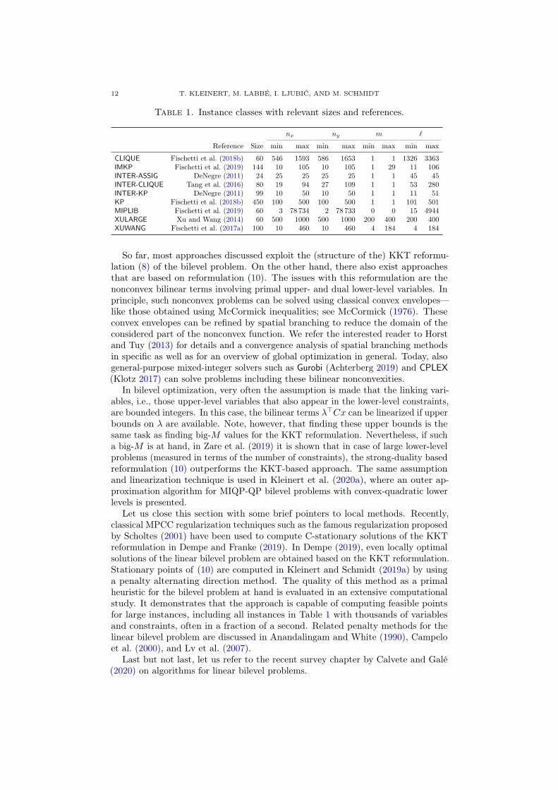
where C is a constraint set containing already added valid inequalities of any type aswell as branching decisions or might be empty. While the inequality can be appliedthroughout the entire branch-and-bound tree, it is shown that it is most effective atthe root node. In Kleinert and Schmidt (2020), it is shown that when equippingboth approaches, the classical big-M approach and an SOS1-approach for the KKTcomplementarity conditions, with the root node inequality, then the two approachesperform very competitive—but the SOS1-approach does not suffer from the possibletheoretical issues of invalid big-M values. The computational study in Kleinert andSchmidt (2020) is based on a LP-LP test set containing 1077 instances; see Table 1.The table shows relevant problem characteristics such as the number of upper-leveland lower-level variables and constraints for various subsets of the instance set. Inaddition, since all LP-LP instances are derived from mixed-integer linear bilevelproblems, the table gives a reference to the original source of each subset. We notethat the approaches tested in Kleinert and Schmidt (2020) are capable of solving1051 out of the 1077 instances within a time limit of 1 h.


Table 1. Instance classes with relevant sizes and references.

nx ny m `

Reference Size min max min max min max min max

CLIQUE Fischetti et al. (2018b) 60 546 1593 586 1653 1 1 1326 3363IMKP Fischetti et al. (2019) 144 10 105 10 105 1 29 11 106INTER-ASSIG DeNegre (2011) 24 25 25 25 25 1 1 45 45INTER-CLIQUE Tang et al. (2016) 80 19 94 27 109 1 1 53 280INTER-KP DeNegre (2011) 99 10 50 10 50 1 1 11 51KP Fischetti et al. (2018b) 450 100 500 100 500 1 1 101 501MIPLIB Fischetti et al. (2019) 60 3 78 734 2 78 733 0 0 15 4944XULARGE Xu and Wang (2014) 60 500 1000 500 1000 200 400 200 400XUWANG Fischetti et al. (2017a) 100 10 460 10 460 4 184 4 184

So far, most approaches discussed exploit the (structure of the) KKT reformu-lation (8) of the bilevel problem. On the other hand, there also exist approachesthat are based on reformulation (10). The issues with this reformulation are thenonconvex bilinear terms involving primal upper- and dual lower-level variables. Inprinciple, such nonconvex problems can be solved using classical convex envelopes—like those obtained using McCormick inequalities; see McCormick (1976). Theseconvex envelopes can be refined by spatial branching to reduce the domain of theconsidered part of the nonconvex function. We refer the interested reader to Horstand Tuy (2013) for details and a convergence analysis of spatial branching methodsin specific as well as for an overview of global optimization in general. Today, alsogeneral-purpose mixed-integer solvers such as Gurobi (Achterberg 2019) and CPLEX(Klotz 2017) can solve problems including these bilinear nonconvexities.

In bilevel optimization, very often the assumption is made that the linking vari-ables, i.e., those upper-level variables that also appear in the lower-level constraints,are bounded integers. In this case, the bilinear terms λ>Cx can be linearized if upperbounds on λ are available. Note, however, that finding these upper bounds is thesame task as finding big-M values for the KKT reformulation. Nevertheless, if sucha big-M is at hand, in Zare et al. (2019) it is shown that in case of large lower-levelproblems (measured in terms of the number of constraints), the strong-duality basedreformulation (10) outperforms the KKT-based approach. The same assumptionand linearization technique is used in Kleinert et al. (2020a), where an outer ap-proximation algorithm for MIQP-QP bilevel problems with convex-quadratic lowerlevels is presented.

Let us close this section with some brief pointers to local methods. Recently,classical MPCC regularization techniques such as the famous regularization proposedby Scholtes (2001) have been used to compute C-stationary solutions of the KKTreformulation in Dempe and Franke (2019). In Dempe (2019), even locally optimalsolutions of the linear bilevel problem are obtained based on the KKT reformulation.Stationary points of (10) are computed in Kleinert and Schmidt (2019a) by usinga penalty alternating direction method. The quality of this method as a primalheuristic for the bilevel problem at hand is evaluated in an extensive computationalstudy. It demonstrates that the approach is capable of computing feasible pointsfor large instances, including all instances in Table 1 with thousands of variablesand constraints, often in a fraction of a second. Related penalty methods for thelinear bilevel problem are discussed in Anandalingam and White (1990), Campeloet al. (2000), and Lv et al. (2007).

Last but not last, let us refer to the recent survey chapter by Calvete and Galé(2020) on algorithms for linear bilevel problems.


4. Bilinear Lower Levels

A bilevel problem for which the lower level contains bilinearities but which is alinear problem when the upper-level variables x are fixed can also be reformulatedas a single-level optimization problem by using any of the two techniques describedin Section 3.2. Pricing problems and Stackelberg bimatrix games constitute twoclasses of bilevel problems that present this feature.

4.1. Pricing Problems. A first bilevel pricing problem with linear constraints,linear upper-level objective and bilinear lower-level objective has been proposed byBialas and Karwan (1984). The following problem considered in Labbé et al. (1998)provides a general framework for pricing:

maxx,y=(y1,y2)

x>y1 (11a)

s.t. Ax ≤ a, (11b)

y ∈ arg miny

{(x+ d1)>y1 + d>2 y2 : D1y1 +D2y2 ≥ b

}. (11c)

The vector y of lower-level variables is partitioned into two sub-vectors y1 and y2,called plans, that specify the levels of some activities such as goods or services. Theupper level influences the activities from plan y1 through a price vector x it chargesto the lower level and maximizes its revenue given by x>y1. The price vector xis subject to linear constraints that may, among others, impose lower and upperbounds on the prices. Vectors d1 and d2 represent linear disutilities faced by thelower level when executing the activity plans y1 as well as y2. Note that d2 may alsoencompass the price for executing the activities not influenced by the upper level.These activities may, e.g., be substitutes offered by competitors for which prices areknown and fixed. The lower level determines its activity plans y1 and y2 to minimizethe sum of total disutility and the price paid for plan y1 subject to linear constraints.Remark that if the model allows negative prices then it implicitly permits subsidies,which may be appropriate, e.g., in the context of a central agency determining taxes.In order to avoid the situation in which the upper level would maximize its profit bysetting prices to infinity for these activities y1 that are essential, one may assumethat the set {y2 : D2y2 ≥ b} is nonempty. Indeed, in this case, there exists a feasiblepoint for the lower level that does not use any activity influenced by the upper level.

We now discuss some interesting geometrical properties of the bilevel pricingproblem. First, remark that the feasible region of the lower level (11c) is independentof the upper-level variables x, which is in contrast to the lower level (7) of theLP-LP problem. Assuming that the feasible region of the lower level is bounded,i.e., a polytope, allows us to conclude that for every upper-level decision the optimalsolution of the lower level is attained at a vertex of the feasible polytope of the lowerlevel. In addition, strong duality holds for every parametric lower level problem (11c).Second, we look at the single-level reformulation of Problem (11) obtained by usingthe KKT conditions of the lower-level problem (11c):

maxx,y=(y1,y2),λ

x>y1 (12a)

s.t. Ax ≤ a, D1y1 +D2y2 ≥ b, (12b)

D>1 λ = x+ d1, D>2 λ = d2, λ ≥ 0, (12c)

λ>(D1y1 +D2y2 − b) = 0. (12d)

Let (y1, y2) be a fixed vertex of the feasible polytope of the lower level. Then, theconstraints of (12) are linear in x and λ, i.e., they constitute a polyhedral set forfixed (y1, y2). By considering all vertices of the lower level, we determine a partitionof the feasible set of Problem (12) into a (possibly exponential) number of polyhedral


cells with the property that all price vectors x belonging to a cell share the samelower-level optimal solution. Some of these cells may be empty. As a consequence,the objective function of the bilevel pricing problem is neither convex nor continuousin x but is linear in each cell.

Formulation (12) contains nonlinear terms both in its objective function (12a)and in constraints (12d). To circumvent the nonlinearity of the latter one mightuse the approach proposed by Fortuny-Amat and McCarl (1981) that is describedin Section 3.3 but to do so, again one needs to bound the dual variables, which isNP-hard in general as mentioned earlier. Another approach consists of replacingthe complementarity constraints by the strong duality condition

(x+ d1)>y1 + d>2 y2 ≤ b>λ.that involve the same bilinear term as the objective function (12a). Grimm et al.(2020) use the latter kind of reformulation for the lower-level problem for particularcases of the above bilevel pricing problem (11) that correspond to different electricityretailer pricing schemes. Zugno et al. (2013), on the other hand, consider a similarelectricity pricing problem but use the KKT optimality conditions and the single-levelreformulation à la Fortuny-Amat and McCarl (1981).

If all vertices of the feasible polytope of the lower level are binary, bilinear termscan be linearized more efficiently when using the approach proposed by McCormick(1976). This particularly applies to lower-level problems that are polynomial graphproblems. Van Hoesel (2008) and Labbé and Violin (2013) present surveys aboutsuch so-called network pricing problems that we briefly sketch in the following.Consider a graph whose arc weights represent travel costs. In the toll settingproblem, the upper level determines the prices (or tolls) of a subset of arcs of anetwork in order to maximize its revenue obtained by collecting tolls paid by thelower level that consists in a given number of users, each one being an independentfollower. Each user selects a path from her origin to her destination that minimizesher disutility given by the sum of the prices of the arcs in the path that are controlledby the upper level plus the total travel costs.

Labbé et al. (1998) show that the toll setting problem with (possibly negative)lower bounds on the prices is NP-hard even for a single user and that it is polynomialin the special case that one single arc is to be priced. Roch et al. (2005) strengthenthe complexity result by showing that the single-user toll setting problem is alreadystrongly NP-hard if all lower bounds on the prices are equal to 0. Joret (2011)shows that the problem is also APX-hard. Labbé et al. (1998) propose an MILPreformulation of the toll setting problem that involves big-M values. Dewez etal. (2008) show how to derive efficient big-Ms and propose valid inequalities thatstrengthen the MILP model. Brotcorne et al. (2001) propose heuristics and Bouhtouet al. (2007) present a preprocessing method to reduce the graph size. Didi-Bihaet al. (2006) and Brotcorne et al. (2011) exploit the fact that revenue maximizingprices that are compatible with a given lower-level solution can be easily determined.They propose exact algorithms as well as heuristics based on multi-path generation.

Heilporn et al. (2010b) and Heilporn et al. (2011) study the particular case inwhich each follower uses at most one arc priced by the leader. Heilporn et al. (2010b)show that the problem is strongly NP-hard. Further, exploiting the fact that thereexists a limited number of feasible solutions for each follower, they provide anMILP formulation based on the optimal value function, a polyhedral study of thisformulation, and provide a complete description of the convex hull of feasible pointsfor the special case of one single follower. In Heilporn et al. (2011), a branch-and-cutprocedure is proposed.

Heilporn et al. (2010a) show the equivalence of this problem with the so-calledproduct line pricing problem. In the upper level of this problem, prices of products


must be determined to maximize total revenue. In the lower level, customers choosethe product that maximizes their welfare given by the difference of their reservationprice (also called willingness to pay) for the product and its price. The productline design and pricing was originally introduced by Dobson and Kalish (1988).Guruswami et al. (2005) show that it is APX-hard. MILP formulations differentthan the one used in Heilporn et al. (2010b) are presented in Shioda et al. (2011),Myklebust et al. (2016), and Fernandes et al. (2016). Moreover, heuristics areproposed in Dobson and Kalish (1993), Shioda et al. (2011) as well as Myklebust etal. (2016). Instance generators that are publicly available are described in Fernandeset al. (2016).

Castelli et al. (2017) show that the special case in which the price of all arcscontrolled by the leader must be equal is polynomial. Furthermore, they also showthat the problem is pseudo-polynomial when arc prices must be proportional totheir length and they also consider a robust variant of these problems. Castelliet al. (2013) apply the model with proportional prices in the context of air trafficmanagement to determine how much Air Navigation Service Providers (ANSPs)should charge airlines to use their airspace.

Marcotte et al. (2009) use the toll setting problem to determine road tolls toregulate the use of roads for hazardous shipments and show that an optimal toll policyis more efficient then a network design approach that determines road segments tobe closed to dangerous materials.

Brotcorne et al. (2008) consider the more general problem in which the leaderfaces a joint design and pricing problem. Here, in the upper-level objective, a fixedcost is incurred for each arc that is installed (and priced) by the leader. The lowerlevel is the same as in the toll setting problems. They show that the couplingconstraints linking the design variables and the user arc choice variables appearingin the lower level can be moved to the upper level. These constraints forbid thefollowers to use arcs that are not installed. Moving them to the upper level isallowed because the leader can prevent the followers to use them by setting theirprice very high. Finally, they suggest a single-level MILP formulation as well asheuristics.

Network pricing problems with different lower-level problems have also beenstudied. Brotcorne et al. (2000) consider a lower level given by an uncapacitatedtransshipment problem and provide an MILP formulation as well as some heuristics.Another variant is obtained by assuming that the lower level selects a minimumspanning tree. Cardinal et al. (2011) show that this problem is APX-hard, whereasMorais et al. (2016) and Labbé et al. (2021) propose different MILP formulations.

4.2. Stackelberg Games. The determination of optimal Stackelberg mixed strate-gies in a two-player normal-form game constitutes another typical bilevel problem inwhich both objectives are bilinear (in both the upper- and lower-level variables) andall constraints are linear. In such a game, two players, say A and B are endowedwith a set of pure strategies I and J with |I| = n, |I| = m. The matrices R = [Rij ]and C = [Cij ] encode the respective utilities when A plays strategy i and B playsstrategy j. A mixed strategy for player A (B) is a probability distribution x (y)over her pure strategy set I (J). Both players want to maximize their respectiveexpected utility given by x>Ry and x>Cy. Now assume that the players choose theirmixed strategy sequentially: A is the leader and plays first, then B, informed of A’sdecision, reacts optimally with respect to her own objective. This is called a generalStackelberg game and the solution, called Strong Stackelberg Equilibrium (SSE), is


given by an optimal solution of the bilevel problem

maxx,y

x>Ry (13a)

s.t. 1>x = 1, x ≥ 0, (13b)

y ∈ arg maxy

{x>Cy : 1>y = 1, y ≥ 0

}, (13c)

in which 1 denotes the vector of all ones in appropriate dimension. The term “strong”stands for the fact that the optimistic version of the problem is considered.

Problem (13) can be solved using linear programming. First notice that for agiven leader’s solution x, the lower level is an LP on the unit simplex. In otherwords, there always exists an optimal solution for the follower that is one of then vertices of the unit simplex. Second, a solution x that maximizes the leader’sutility and for which some solution y, with yj = 1 for some j ∈ J , is optimal for thefollower can be found by solving problem (13) whose objective function is x>R·jand in which the lower-level problem (13c) is replaced with

x>C.·j′ ≤ x>C·j for all j′ ∈ J.Hence, solving this LP for every possible pure strategy of the follower and retainingthe one that yields the highest utility for the leader provides an SSE; see Conitzerand Sandholm (2006).

Problem (13) can be adapted to the case in which the leader does not know thefollower’s preferences over the outcomes of the game with certainty. This is doneby considering different types k ∈ K of followers. In this case, the game is calledBayesian. Utility matrices Rk and Ck are then given for each follower type k as wellas a probability πk that the type of the follower is indeed k. The leader’s expectedutility is then equal to

∑k∈K π

kx>Rkyk and a lower-level problem

yk ∈ arg maxyk

{x>Ckyk : 1>yk = 1, yk ≥ 0

}is introduced for each follower type. A Bayesian Stackelberg game can be seen asa regular Stackelberg game in which the set of pure strategies of the follower iscomposed of all n|K| possible combined choices of pure strategies of the differentfollower types; see Harsanyi and Selten (1972). As a consequence, an SSE in aBayesian Stackelberg game can be determined in polynomial time when the numberof types is fixed. If not, the problem is NP-hard; see again Conitzer and Sandholm(2006).

The bilevel optimization problem that determines an SSE of a general BayesianStackelberg game can be reformulated as a single-level MILP. In fact any of thethree approaches consisting in using KKT conditions, strong duality, or the optimalvalue function leads to an equivalent single-level reformulation. Then, to circumventthe bilinearities in the objective functions of both levels, one may exploit the factthat there always exists an optimal follower’s response that is binary, i.e., it isa pure strategy. Paruchuri et al. (2008), Kiekintveld et al. (2009), and Yin andTambe (2012) propose models based on these principles. The LP relaxation of theformulation proposed by Yin and Tambe (2012) is the strongest and provides acomplete description of the convex hull of feasible points in the case of a singlefollower. See Casorrán et al. (2019) for comparison of the three above mentionedformulations from both theoretical and computational point of views. On the otherhand, decomposition methods scale better when the problem involves many resourcesand/or follower types. In this perspective, Paruchuri et al. (2008) propose a solutionapproach involving Benders decomposition and Jain et al. (2010) and Lagos et al.(2017) use column generation.


Stackelberg games have been shown to be useful for many real-world applicationsin security domains. In these so-called Stackelberg security games, the leader (de-fender) places security resources (e.g., guards) at various potential targets (possiblyin a randomized manner), and then the follower (attacker) chooses a target to attack;see e.g. Jain et al. (2013). Examples of such applications include disrupting drugtrafficking networks (Washburn and Wood 1995), assigning Federal Air Marshals totransatlantic flights (Pita et al. 2008), determining randomized port and waterwayspatrols for the U.S. Coast Guard (Shieh et al. 2012), preventing fare evasion inpublic transport systems (Yin et al. 2012), protecting endangered wildlife (Yanget al. 2014), or coordinating resources to organize patrols of the Chilean nationalpolice force (Bucarey et al. 2019). See also the book edited by Tambe (2011) thatdescribes many applications and the survey by Sinha et al. (2018) that presentsrecent advances in Stackelberg security games. In these security games, playinga mixed strategy of the defender is particularly appropriate because even if theattacker is aware of this mixed strategy, she does not know which pure strategy willactually be put in action when she attacks. This is especially relevant when thegame is played in a repeated way, e.g., every day.

A common feature of Stackelberg security games is that pure strategies of theleader consist in allocating several resources to protect targets, leading to anexponential number of such pure strategies. In the simplest case, J represents aset of targets that may be attacked and each target attack corresponds to a purestrategy of the attacker. Further, assume that the defender has a set of m < n(identical) resources available to cover these targets. The possible pure strategies ofthe defender consist in all subsets of J of cardinality at most m. As a consequence,any of the formulations proposed for finding an SSE in a general Stackelberg gamebecomes rapidly intractable when the number of targets and/or resources increase.

To alleviate this situation, Kiekintveld et al. (2009) propose to encode a leader’smixed strategy by a vector x whose entries xj represent the marginal probabilitiesof covering each target j in this mixed strategy. The marginal probability of atarget is equal to the sum of the probabilities of the pure strategies covering thesaid target. In other words, a vector x of marginal probabilities is a point belongingto the convex hull of the binary vectors corresponding to all possible pure strategies,i.e., all binary vectors with at most m entries equal to 1. It can be readily seenthat this convex hull is

{x : 1>x ≤ m, 0 ≤ x ≤ 1

}. Indeed, the constraint matrix

is totally unimodular so that all the vertices of this polytope are binary vectors.Further, as explained in Kiekintveld et al. (2009), the mixed strategy correspondingto a given vector of marginal probabilities can be retrieved in polynomial time sinceit amounts to solve a linear system with a polynomial number of constraints. In thecontext of a scheduling problem, McNaughton (1959) proposes an alternative andfaster polynomial procedure.

Another common feature of Stackelberg security games is that the utility of boththe defender and the attacker depend only on whether the target that is attacked isprotected or not. There are two cases, depending on whether or not the target iscovered by the defender. The defender’s utility for an uncovered attack of type kon target j is denoted Dk(j|u) and for a covered attack of type k it is denoted asDk(j|c). Similarly, Ak(j|u) and Ak(j|c) represent the type k attacker’s utilities.With these new notations at hand, one can formulate the following bilevel problem


that determines an SSE in a Bayesian Stackelberg security game:

maxx,y

∑k∈K

πk∑j∈J

(xjDk(j|c) + (1− xj)Dk(j|u))ykj

s.t. 1>x ≤ m, 0 ≤ x ≤ 1,

yk ∈ arg maxyk

∑j∈J

(xjAk(j|c) + (1− xj)Ak(j|u))ykj : 1>y = 1, y ≥ 0

.

Three single-level MILP reformulations similar to the ones proposed for generalStackelberg games can be derived for this problem; see Casorrán et al. (2019). Theauthors also compare them with extended formulations that involve all possiblemixed strategies, i.e., formulations of the general Stackelberg game version of suchsecurity games.

Other variants of Stackelberg security games involve more sophisticated purestrategies of the leader. Resources can be heterogeneous meaning that each resourcecan only cover a subset of targets. Resources can cover at once a subset of targets,called schedule. Korzhyk et al. (2010) investigate the complexity of such variantswith one type of follower. They show that a Stackelberg security game withhomogeneous resources is polynomial if the schedules have size at most 2 and isNP-hard otherwise. When resources are heterogeneous, they show that the problemis polynomial when schedules have size 1 and NP-hard otherwise. Jain et al. (2010)propose a branch-and-price approach for such variants by iteratively generatingcolumns representing pure strategies of the leader. Finally, Letchford and Conitzer(2013) study the complexity of the case of Stackelberg security games in whichthe targets are vertices of a graph and schedules are subgraphs with a particularstructure such as path or tree.

5. Mixed-Integer (Non)Linear Lower Levels

In this section, we focus on a general bilevel MILPs, which are defined as

minx∈X,y

c>x x+ c>y y (14a)

s.t. Ax+By ≥ a, (14b)

y ∈ arg miny∈Y

{d>y : Cx+Dy ≥ b

}, (14c)

where the vectors cx, cy, d, a, b and matrices A,B,C,D are defined as in Section 3.The sets X and Y specify integrality constraints on a subset of x- and y-variables,respectively.

The HPR’s feasible region of this bilevel MILP is, as usual, defined as the set ofpoints (x, y) ∈ X × Y satisfying all constraints of the upper and lower level, i.e.,

H := {(x, y) ∈ X × Y : Ax+By ≥ a, Cx+Dy ≥ b} .The inducible region of a bilevel MILP consists of all bilevel feasible points, i.e., allpoints (x, y) ∈ H for which for a given x, the vector y is an optimal solution of thelower-level problem. This means,

d>y ≤ ϕ(x),

holds. Here, ϕ(x) again is the optimal value of the lower-level problem, which isdefined as

ϕ(x) = miny∈Y

{d>y : Dy ≥ b− Cx

}. (15)

The value function ϕ(x) thus corresponds to a parametric MILP, and hence it isnonconvex, not continuous, and in general very difficult to describe. Moreover, in


contrast to bilevel LPs, it is NP-hard to check whether a given point (x, y) is afeasible solution of the bilevel MILP. Jeroslow (1985) showed that k-level discreteoptimization problems are Σp

k-hard, even when the variables are binary and allconstraints are linear. This means that, e.g., a discrete bilevel optimization problemcan be solved in nondeterministic polynomial time, provided that there exists anoracle that solves problems that are in NP in constant time.

The inducible region of the bilevel MILP is contained in the set H, and therefore,minimizing the objective function of the upper level over the set H (which representsanother MILP) provides a valid lower bound for the bilevel MILP. Consequently,solving the LP-relaxation of the HPR provides another (and usually much weaker)lower bound of the bilevel MILP.

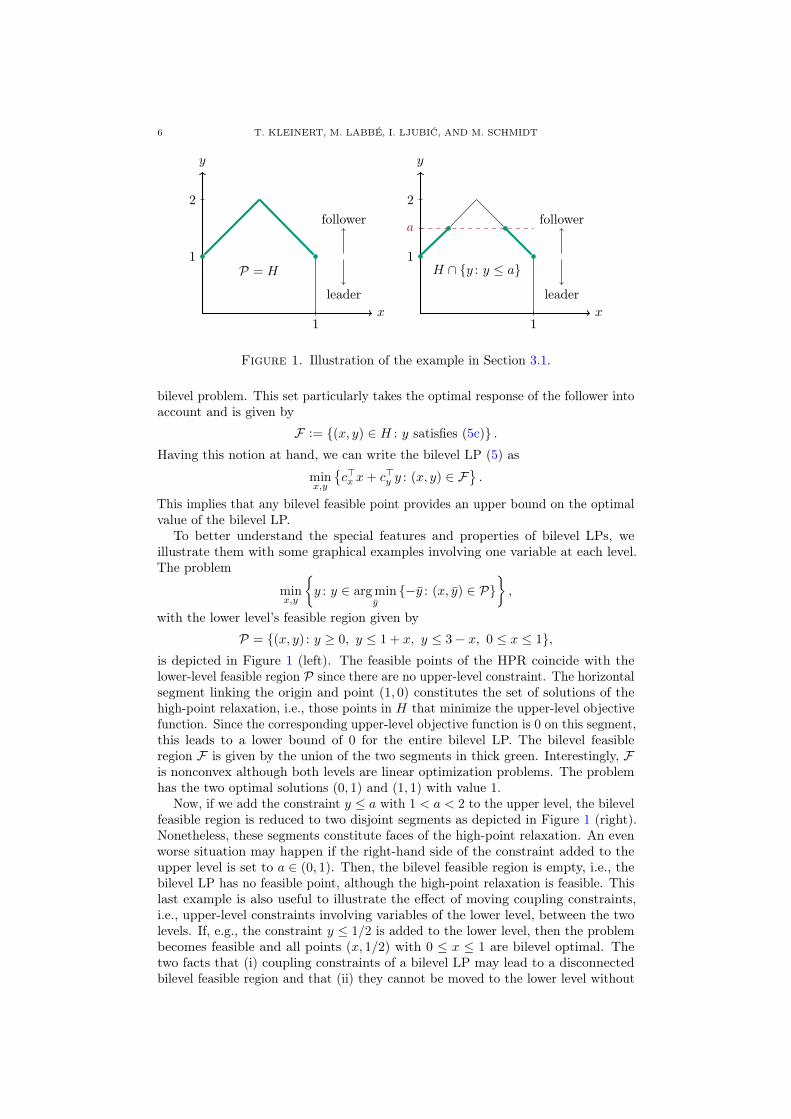
Moore and Bard (1990) initiated the studies of bilevel optimization problemsinvolving discrete variables. Their illustrative example (cf. Figure 2) is frequentlyused in the literature to highlight the major differences and pitfalls arising in discretebilevel optimization. Since then, studies have been carried out considering onlyspecial cases, e.g., by assuming binary variables at both levels or by consideringpurely linear problems at the lower level. Exact MILP-based procedures for thegeneral case in which both the upper and the lower level are MILPs have beenmainly studied in the last decade.

5.1. General Properties. The following example is provided by Moore and Bard(1990):

minx∈Z,y∈Z

{−x− 10y : y ∈ arg min

y∈Z{y : (x, y) ∈ P}

},

where P is a polytope defined by

−25x+ 20y ≤ 30, x+ 2y ≤ 10, 2x− y ≤ 15, 2x+ 10y ≥ 15.

The HPR of this problem is an integer linear problem, whose feasible region isdepicted in Figure 2. The unique optimal solution for this example is the point(2, 2), which is in the interior of the convex hull of the HPR. This is in contrast tobilevel LPs, whose optimal solution is always a vertex of the HPR; see Section 3.The example also shows that relaxing the integrality constraints for the lower-levelproblem does not provide neither lower nor upper bounds for the bilevel MILP.Dashed lines in Figure 2 correspond to the inducible region of the problem in whichthe integrality constraints for both the upper-level and the lower-level variables arerelaxed. In general, such obtained set does not even have to contain a single bilevelfeasible point.

Attainability of Optimal Solutions. In Vicente et al. (1996), the authors con-sider three cases of bilevel MILPs and study the following different assumptions:

(i) only upper-level variables are discrete,(ii) all upper- and lower-level variables are discrete, and(iii) only lower-level variables can take discrete values.

Assuming that all discrete variables are bounded and that the inducible region isnonempty, they show that for Case (i) and (ii), an optimal solution always existsand that (i) can be reduced to a linear bilevel program (cf. Section 3), whereas (ii)can be reduced to a linear trilevel problem. However, for Case (iii), Moore and Bard(1990) and also Vicente et al. (1996) provided examples that demonstrate that thebilevel feasible region may not be closed, and hence, the optimal solution may notbe attainable. The following simpler example (see Figure 3) is due to Köppe et al.


x

y

1 2 3 4 5 6 7 8

1

2

3

4

Figure 2. Example of a bilevel MILP: Discrete points are feasiblefor the high-point relaxation. The point (2, 4) is the optimal solutionof the high-point relaxation and (2, 2) is the optimal solution ofthe bilevel MILP. Triangles represent bilevel feasible solutions anddashed lines represent the feasible region of the bilevel LP in whichthe integrality constraints on the upper- and lower-level variablesare relaxed.

y

x1

1

Figure 3. The attainability counterexample by Köppe et al. (2010)

(2010):

inf0≤x≤1,y

{x− y : y ∈ arg min

y′∈Z{y : y ≥ x, 0 ≤ y ≤ 1}

},

which is equivalent toinfx{x− dxe : 0 ≤ x ≤ 1} .

In this problem, the infimum is -1, which is never attained. In the existing literatureon bilevel MILPs, it is therefore frequently assumed that the linking variables arediscrete. We recall that nonlinking upper level variables can be moved to the lowerlevel (Bolusani and Ralphs 2020; Tahernejad et al. 2020), which effectively translatesthe latter assumption into “all upper-level variables are discrete”. Alternatively, forbilevel MILPs with continuous linking variables, methods that achieve ε-optimalsolutions are considered if the optimal solution cannot be attained; see, e.g., Zengand An (2014).

Unboundedness of the Lower-Level Problem. A common assumption foralgorithms dealing with bilevel MILPs is that the feasible region of the HPR iscompact. Sometimes, this condition is relaxed and it is only assumed that discretevariables are bounded. For the latter case, Xu and Wang (2014) demonstrate that


the unboudedness of the optimal HPR value does not reveal the nature of theunderlying bilevel problem. It can happen that the underlying bilevel MILP isinfeasible, unbounded, or admits an optimal solution; see also Section 3 for anillustrative example. Xu and Wang (2014) (cf. Lemma 2) also show that if the lowerlevel MILP (15) is unbounded (i.e., ϕ(x) = −∞ for a certain x from the HPR’sfeasible region), then the bilevel MILP (14) is infeasible. Later, Fischetti et al.(2018a) showed that for any bilevel MILP whose HPR value is unbounded, one candetect upfront whether the lower-level problem is unbounded or not. To this end,it is sufficient to solve a single LP (not depending on x) in a presolve phase. Thesolution of this LP, cf. Theorem 1 of Fischetti et al. (2018a), provides a direction(if such exists) in which the lower-level problem defined by (15) is unbounded—nomatter the choice of the vector x from the HPR’s feasible region.

5.2. Generic Approaches for Bilevel MILPs. Most of the exact methods stud-ied in the literature start with solving the high-point relaxation, i.e., min{c>x x +c>y y : (x, y) ∈ H}, and continue by discarding bilevel infeasible solutions by branch-ing, by adding cutting planes, by approximating the value function ϕ(x) givenin (15), or by a combination of all of them. In the following, we review thesemethods and point out to their differences.

Branch-and-Bound Methods. In their seminal paper, Moore and Bard (1990)develop the first branch-and-bound method for discrete bilevel optimization. Theiralgorithm terminates after a finite number of iterations if all upper-level variablesare integer or all lower-level variables are continuous (assuming an optimum exists).In addition, the authors assume that the HPR’s feasible region is compact andthat there are no coupling constraints at the upper level. The authors point outthat two of the three standard B&B fathoming rules for mixed-integer optimizationare not valid in the bilevel context and discuss further computational challengesof solving discrete bilevel problems. Bard and Moore (1992) then propose anotherexact algorithm for bilevel MILPs assuming that all variables (x, y) are binary.

Fischetti et al. (2018a) developed another branch-and-bound method that worksfor mixed-integer upper- and lower-level problems and allows coupling constraints atthe upper level. The major assumption is that the discrete variables are bounded andthat the linking variables are discrete. Necessary modifications of a standard B&B-based MILP solver are introduced to properly handle branching, node evaluation,and fathoming rules. The method checks unboundedness of the lower-level problemin a presolve phase; see Section 5.1. Together with Xu and Wang (2014), see below,the proposed B&B algorithm is one of the few methods that return a provablyoptimal solution (if such exists) within a finite number of iterations without assumingthat the HPR’s feasible region is compact. Instead, only the discrete variables needto be bounded.

Parametric Integer Programming Methods. Faísca et al. (2007) assume thatdiscrete variables of the bilevel MILP are binary and use parametric programmingto develop an exact method that works in two phases. In the first phase, all Klower-level solutions are enumerated using parametric integer programming. Then,each solution is plugged into the upper-level problem, yielding K single-level MILPproblem reformulations, from which the best one represents the global optimum.The approach is picked up and extended to bilevel MIQPs in Avraamidou andPistikopoulos (2019a). The authors also provide a computational study for bilevelMILPs and bilevel MIQPs. A more detailed description of the implementation canbe found in Avraamidou and Pistikopoulos (2019b).

Köppe et al. (2010) also approach bilevel MILPs from the parametric programmingperspective. They view the lower-level problem as a parametric (integer) program


whose right-hand side is parameterized by x. The authors propose an algorithm thatruns in polynomial time for a fixed dimension ny of the lower-level problem and forthe case that the linking variables are continuous. In case the linking variables arediscrete, the authors show that there exists an algorithm that runs in polynomialtime for a fixed dimension nx+ny. The algorithm applies binary search by targetingthe optimal value of the bilevel MILP.

Multi-Way Branching. Xu and Wang (2014), see also the PhD thesis by Xu(2012), apply a multi-way branching method to solve bilevel MILPs in which allleader variables are required to be integer and bounded. The algorithm solves aseries of MILPs obtained by restricting the values of slack variables of the lower-levelconstraints. Another enhanced version of this method, which provides a heuristicsolution in the case that the lower-level problem has multiple optimal solutions, isgiven by Liu et al. (2020b).

In their “watermelon algorithm”, Wang and Xu (2017) exploit multi-way branchingto “carve out” bilevel infeasible points from the feasible region of the HPR. Whenevera bilevel infeasible point (together with a polyhedron around it that contains nobilevel feasible points) is discovered, it is discarded by decomposing the search spaceinto a family of smaller polyhedra, which are then solved in a recursive fashion. Twodifferent ways to determine the bilevel-free polyhedron around a given infeasiblepoint are proposed along with MILP-based procedures for their determination.

Branch-and-Cut Methods. By extending the ideas from Moore and Bard (1990),DeNegre and Ralphs (2009), see also the dissertation by DeNegre (2011), developan MILP-based branch-and-cut approach. Their method does not allow for anycontinuous variables and coupling constraints at the upper level. Bilevel infeasiblesolutions are cut off on the fly by adding “integer no-good cuts” that exploit theintegrality property of the upper- and lower-level variables. These cuts are guaran-teed to separate bilevel infeasible points from the convex hull of the bilevel feasibleregion. An extension of this method that allows for a mixed-integer setting at bothlevels is given by Tahernejad et al. (2020). The authors provide a comprehensive im-plementation that integrates many computational and algorithmic features proposedin the recent literature on bilevel MILPs.

A cutting plane method for bilevel MILPs in which all variables are discrete isgiven by Caramia and Mari (2015). The authors solve the HPR and utilize a variantof “no-good” constraints (involving big-Ms and `∞-norms) to cut off nonoptimalresponses from the follower on the fly. They also propose a B&C method with aspecific branching rule derived from rounding the value of the optimal follower’sresponse.

Dempe and Kue (2017) consider two special cases of bilevel MILPs: (i) bothlevels contain discrete variables only and the leader influences the objective of thefollower (i.e., the objective function is bilinear), and (ii) only the lower level containsdiscrete variables and the leader influences the right-hand-side of the follower. Forthe former case, the authors propose a B&C algorithm based on covering-type validinequalities. For the latter case, the authors exploit the structural properties of thevalue function and derive an iterative MILP-based procedure in which the valuefunction is refined. The methods have been illustrated on two small examples.

To enhance the performance of their basic B&B method, Fischetti et al. (2018a)introduce intersection cuts to separate integer bilevel infeasible points, thus obtaininga B&C approach for bilevel MILPs. These cuts, which are traditionally used formixed-integer programming (see, e.g., Balas (1971)) are used here for the first timeto solve bilevel MILPs: LP-optimal solutions (being integer but bilevel infeasible)are cut off by deriving a cut in which the LP-cone of this solution is intersected with


a convex set that contains no bilevel feasible points. In a follow-up article, Fischettiet al. (2017a) provide additional computational techniques to further improve theirB&C method. These techniques include new ways to derive intersection cuts, followerupper-bound cuts and variable fixing based on the properties of the lower-levelproblem. The results also include hypercube intersection cuts, which can deal withlower levels with continuous variables. The authors conducted a computationalstudy on a set of benchmark instances shown in Table 1 (except CLIQUE andIMKP) and optimal solutions have been reported for 822 out of 874 instances. Thecode of Fischetti et al. (2017a) is publicly available (Fischetti et al. 2017b), andrepresents the current state-of-the-art exact method for general bilevel MILPs. Thecode is integrated within the commercial solver CPLEX. An alternative open-sourceimplementation that includes features of Fischetti et al. (2017a), but also manyadditional ones, has been developed by Tahernejad et al. (2020) and is availableonline (Ralphs 2018). Unsurprisingly, specialized approaches for solving particularinterdiction problems, like those of Fischetti et al. (2019) and Furini et al. (2020b),are outperforming the generic approaches by Fischetti et al. (2017a) and Tahernejadet al. (2020) on interdiction instances such as INTER-KP, KP, INTER-CLIQUE, andCLIQUE; see Table 1.

Benders-like Decomposition. A Benders-like decomposition scheme for generalbilevel MILPs is given in Saharidis and Ierapetritou (2009), assuming that the HPR’sfeasible region is compact. Valid Benders-like cuts are derived by fixing the valueof integer variables at the master level and using the active-set strategy togetherwith the KKT reformulation of the resulting continuous lower-level problem. Thealgorithm terminates when an ε-optimal solution is achieved.

In a recent article by Bolusani et al. (2020), the authors make a parallel betweenbilevel MILPs and two-stage stochastic MILPs with recourse. By exploiting theircommon mathematical structure given by the value-function reformulation and usingthe MILP-duality theory, a unified algorithmic framework is provided. In Bolusaniand Ralphs (2020), a Benders-like decomposition to approximate the value functionand a cutting-plane method are discussed as two possible solution strategies.

Other Approaches. Zeng and An (2014) proposed a single-level reformulationand a decomposition algorithm based on a column-and-constraint generation schemefor general bilevel MILPs. The authors even allow the linking variables of the leaderto be continuous. Under the assumption that the optimal solution is attainable, thealgorithm finds an optimal solution. Otherwise, it finds an ε-solution. Their ideais picked up by Yue et al. (2019) who propose to project out integer variables ofthe lower-level problem and work with KKT conditions of the remaining continuouslower-level problem.

Another alternative approach for binary lower-level problems is recently proposedby Shi et al. (2020). The authors consider bilevel MILPs in which the lower-levelvariables are all binary. The method is based on the k-optimality of the lower-level solution: It is a relaxation of the lower-level problem in which the follower’sresponse is accepted by the leader as long as it is within the k-Hamming distanceneighborhood of any bilevel feasible solution. This way, it is possible to model notcompletely rational decisions of the follower. The authors provide a hierarchy ofdecisions linked with the value of k, along with a hierarchy of upper and lowerbounds of the original bilevel problem, which corresponds to k = 0.

5.3. Bilevel MINLPs. For single-level nonconvex mixed-integer optimization prob-lems, one can only expect to compute ε-optimal solutions. Thus, the same alsoholds for nonconvex mixed-integer bilevel problems. We refer to Definition 3 inMitsos et al. (2008) for a formal definition of ε-optimality in the bilevel context and


discuss some approaches for bilevel problems with general nonconvex mixed-integerlower-level problems in the following.

In Mitsos (2010), general bilevel MINLPs with continuity assumptions on allfunctions are considered. In addition, all variables are assumed to be bounded. Thestated approach is an extension of the method proposed in Mitsos et al. (2008) thatdealt with purely continuous bilevel problems. In turn, the latter paper builds ontheoretical developments in Mitsos and Barton (2006). The key idea is to exploitestimates on the optimal value function of the lower level, which requires the globalsolution of MINLPs as subproblems. The approach is shown to terminate in finitetime and an implementation of the approach is evaluated on a small test set.

In a series of papers, the so-called branch-and-sandwich approach for bilevelMINLPs is developed. The main idea is to subsequently compute tightened boundson the optimal value function (3) and on the upper-level objective function value.Starting with continuous but nonconvex lower-level problems in Kleniati and Adjiman(2014b) and a numerical evaluation thereof in Kleniati and Adjiman (2014a), theapproach is extended to the mixed-integer case in Kleniati and Adjiman (2015). Theapproach stated in the latter paper is applicable to problems with twice continuouslydifferentiable functions F , f , G, and g and requires bounds on all variables. Inthis setting, the branch-and-sandwich approach terminates in finite time. Recently,novel bounding schemes for this approach have been published in Paulavičius andAdjiman (2020) and further implementation details can be found in Paulavičiuset al. (2020). Due to the general hardness of the problems under consideration,the computational study in Kleniati and Adjiman (2015) deals with rather smallproblems with up to 12 variables and 7 constraints.

A different setting is considered in Lozano and Smith (2017a). All functions F ,f , G, and g are continuous but possibly nonconvex. In addition, the constraintfunctions G and g need to be separable in x and y, i.e., they have to be of the formG(x, y) = G1(x)+G2(y) and g(x, y) = g1(x)+g2(y). Under the assumptions that (i)the upper- and lower-level feasible regions are compact, (ii) g1(x) is integer-valuedfor all x, and (iii) all upper-level variables x are integers, the authors derive a finitesolution approach based on the value-function reformulation (4). In particular, thisapproach is also capable of solving the pessimistic variant.

6. Interdiction Problems

Interdiction games are a special class of bilevel problems that aim at monitoringor halting an adversary’s activity in a given environment. They are used to modeldefender-attacker settings in which the attacker (the follower) optimizes someobjective such as a shortest path or a maximum flow in a network (see, e.g., Israeliand Wood (2002)), or maximizes the profit of the items that can be packed ina knapsack (Caprara et al. 2014; Fischetti et al. 2019). The defender, who actsas the leader, has limited resources to protect the environment, e.g., by disablingthe vertices/edges in a network or by changing their capacity, or by removing theknapsack items, to achieve the worst possible outcome for the attacker. Besidesmilitary applications, interdiction problems are extremely important in controllingthe spread of infectious diseases (Assimakopoulos 1987; Furini et al. 2021; Shenet al. 2012), spread of fake news in social networks (Baggio et al. 2021), in counter-terrorism and in monitoring of communication networks (Wang et al. 2016).

Interdiction problems follow the common structure of bilevel problems withoutcoupling constraints,

minx∈X,y∈S(x)

{F (x, y) : G(x) ≥ 0} ,


where constraints G(x) describe some restrictions on the solution of the leader,typically including some budget or resource constraints, and S(x) represents theset of optimal solutions of the x-parameterized lower-level problem. Interdictionproblems model zero-sum Stackelberg games, i.e., they correspond to a competitivesetting in which the leader and the follower have diametrically opposed objectivefunctions:

F (x, y) = −f(x, y).

This is why interdiction problems can be alternatively stated as

minx∈X{ϕ(x) : G(x) ≥ 0} , (16)

where the follower’s problem is stated in its maximization form:

ϕ(x) = maxy∈Y{f(x, y) : g(x, y) ≥ 0} . (17)

The leader prevents certain activities of the follower by reducing the availabilityof some objects or resources—for example, items or nodes/edges in a network. Basedon the relationships between the functions f and g and the nature of the leader’svariables x, we make the following distinction.

Discrete Interdiction. In the discrete interdiction setting given below, the linkingvariables xi are binary, and they are set to one if and only if the respective object i isunavailable for the follower. Thus, the objective function f(x, y) = d>y is typicallylinear and the constraints g(x, y) ≥ 0 in (17) are replaced by:

yi ≤ Ui(1− xi), i ∈ Nx, (18a)g(y) ≥ 0, (18b)

where Ui represents the default upper bound for the follower variable yi (modelingthe availability of object i at the lower level), Nx ⊆ {1, . . . , nx} is the index set ofthe binary linking variables of the leader, and g : Rny → R` are constraints thatimpose further restrictions on the follower’s solution. To simplify the exposition, inthe remainder of this section we assume that ny = |Nx|.

Continuous Interdiction. In the continuous interdiction setting, the linkingvariables xi are continuous (i.e., 0 ≤ xi ≤ 1 for i ∈ Nx) and they model a continuousincrease of costs (or reduction of available capacities) imposed on the interdictedobjects. For example, in max-flow interdiction settings, the leader is given a limitedbudget to reduce the available capacity of arcs/vertices, while the follower tries tomaximize the flow in the resulting network; see, e.g., Lim and Smith (2007) andWood (1993) and the further references therein. Alternatively, in the shortest-pathinterdiction (see, e.g., Israeli and Wood (2002)), the leader can increase the cost ofarcs traversed by the follower and in this case, the constraints g(x, y) ≥ 0 in (17)are replaced by g(y) ≥ 0 and the objective function of the follower f(x, y) becomesbilinear, i.e.,

f(x, y) =∑i∈Nx

yi(di + δixi), (19)

as it now encodes the increase of arc costs (modeled by δ) caused by the leader.Finally, one can also consider discrete interdiction problems with bilinear objectivefunctions.

By the nature of the objective function, there is no distinction between optimisticand pessimistic solutions. It is also commonly assumed that the available budget ofthe leader is limited, so that the follower’s problem (17) stays feasible.

In some very special cases, when the interdiction problem can be modeled as abilevel LP, the problem is polynomially solvable; see, e.g., Fulkerson and Harding(1977), where it is shown that continuous interdiction of the shortest-path problem


can be equivalently stated as a minimum cost flow problem. However, discreteinterdiction of the shortest-path problem in which the leader chooses k arcs tointerdict (i.e., G(x) ≥ 0 translates into 1>x ≤ k), already is NP-hard (Ball et al.1989). The latter problem is frequently referred to as the k-most-vital arcs problem.Just like for general bilevel MILPs, if the follower solves an NP-hard problem (e.g.,the maximum knapsack problem or the maximum clique problem), the correspondinginterdiction problem turns out to be Σp2-hard (Caprara et al. 2014; Rutenburg 1994).

6.1. Commonly Studied Interdiction Problems. We provide below a classifica-tion of interdiction problems based on the structures of the encompassed lower-levelproblems.

Network Interdiction with Polynomial Lower-Level Problems. These prob-lems model some of the most traditional and oldest applications arising in the areasof military or homeland security. Besides interdiction of shortest paths (Israeli andWood 2002) or maximum flows (Akgün et al. 2011; Cormican et al. 1998; Janjarassukand Linderoth 2008; Wood 1993), problems also have been studied in which thefollower solves the spanning tree (Bazgan et al. 2013; Lin and Chern 1993) or themaximum matching problem (Zenklusen 2010).

Mixed-Integer Linear System Interdiction Problems. These are interdictionproblems in which the lower level is an MILP. They were first studied in the PhDthesis of Israeli (1999) and later in the PhD thesis of DeNegre (2011). One ofthe most studied (and structurally easiest) variants is discrete interdiction of themaximum knapsack problem, in which the leader and the follower have a knapsackof their own, and the follower can only choose from those items that are not takenby the leader. Complexity results for this problem are given in Caprara et al.(2014), whereas tailored exact methods have been developed in Caprara et al. (2016),Della Croce and Scatamacchia (2019), and Fischetti et al. (2019); see also PhDthesis by Silva Carvalho (2016). The problem’s extension in which the leader and thefollower solve a multidimensional knapsack problem has been addressed in Fischettiet al. (2019). For other variants of more general bilevel knapsack problems (that donot belong to the interdiction setting) see the PhD thesis by Silva Carvalho (2016)and the further references therein.

Facility location with interdiction has been studied as well. Scaparra and Church(2008) investigate the problem in which the leader is concerned with protecting alimited number of facilities, assuming the follower will attack a fixed number of themin order to maximize the transportation cost between the clients and the remainingoperational facilities. In Zhang et al. (2016), the leader locates a fixed number offacilities first, followed by the follower, who is prohibited to use the same location asthe leader. Both players face disruption risks while trying to maximize the marketshare, assuming that each customer patronizes the nearest open facility.

Interdiction problems on networks in which the follower solves an NP-hardproblem also fall into this category. These problems include interdiction of the cliquenumber (Furini et al. 2019, 2020b; Rutenburg 1994), or interdiction of independentsets and vertex covers (Bazgan et al. 2011).

Blocking Problems. Closely related to interdiction problems are the so-calledblocking problems in which the leader wishes to minimize the cost of blocking theactivities of the follower, while ensuring the optimal follower’s response will bebounded by a user-defined threshold r ∈ R:

minx∈X

{c>x x : ϕ(x) ≤ r, G(x) ≥ 0

}.


When blocking the maximum number of cliques, e.g., the leader minimizes the(un)weighted sum of vertices/edges to remove from the graph, so that the maximum(weighted) clique in the remaining graph is bounded from above by a given integer(Pajouh 2020; Pajouh et al. 2014). The blocking of vertices or edges has been studiedwith respect to other graph optimization problems such as the maximum matchings(Zenklusen et al. 2009), shortest paths (Golden 1978), spanning trees (Bazgan et al.2013), or dominating sets (Pajouh et al. 2015).

Most exact methods for blocker problems share similarities with the methodsderived for interdiction problems, which is why we focus on the latter ones in theremainder of this section.

6.2. Methods. The specific structure of interdiction problems can be exploited indifferent ways to derive problem-tailored exact approaches. We summarize genericstrategies used to solve interdiction problems to optimality.

Dualization. When the follower’s problem corresponds to a linear optimizationproblem, duality theory can be exploited to derive a single-level reformulation. If theleader influences the objective function of the follower, like in the bilinear objectivefunction (19), we first dualize the lower-level problem for a given value of x. Thatway, we get rid of the bilinear terms and obtain a single-level formulation (see, e.g.,Israeli and Wood (2002) for the shortest path interdiction) involving variables x ofthe leader and dual variables associated to constraints of the follower’s problem (17).

If the feasible region of the lower level is influenced by the leader, such as in (18),after dualizing the lower-level problem, the resulting single-level reformulation againoptimizes over x and dual variables associated to each constraint of the follower’sproblem. However, its objective function involves bilinear terms in which x-variablesare multiplied with continuous variables of the follower’s dual problem. When dealingwith discrete interdiction problems, these bilinear terms are typically linearizedusing McCormick’s inequalities (McCormick 1976), resulting in a single-level MILPproblem reformulation; see, e.g., the seminal work by Wood (1993) where thistechnique is applied for the maximum-flow interdiction problem. For continuousx-variables, a specialized exact method has been proposed by Lim and Smith (2007)assuming that G(x) ≥ 0 models a budget constraint, exploiting the fact that atmost one of the x-components will be fractional in an optimal interdiction strategy.

Penalization. An alternative way to deal with constraints of Type (18a) in adiscrete interdiction setting is to relax them into

yi ≤ Ui, i ∈ Nx, (20)

and penalize the use of the object i, whenever xi = 1 for an i ∈ Nx. This canbe achieved by introducing coefficients Mi, i ∈ Nx, and by replacing the linearobjective function d>y of the follower by∑

i∈Nx

yi(di −Mixi).

Due to the fact that xi ∈ {0, 1}, the coefficients Mi have to be sufficiently largeto ensure that there always exists an optimal solution of the modified follower’sproblem in which xi = 1 implies yi = 0 for all i ∈ Nx; see, e.g., Smith and Song(2020) and Wood (2011) and further references therein.

When the lower-level problem is linear, this transformation allows one to useduality theory and reformulate the problem as a single-level problem, followingthe same approach as for the bilinear objective function (19) described above. Ifthe lower-level problem is discrete (and NP-hard), one can apply a Benders-likedecomposition approach instead.


Benders-like Decomposition. For linear lower-level problems, the value of Mi

in the penalization approach is chosen as an upper bound of the dual variableassociated to constraint (18a); see, e.g., Brown et al. (2006), Lim and Smith (2007),and Wood (2011).

Israeli (1999) proposes to use the penalty function to reformulate interdictionproblems whose lower-level problem is an MILP. The lower-level problem is thenconvexified using the fact that its feasible region does not depend on x anymoreand, hence, the value function can be restated as

ϕ(x) = max

{∑i∈Nx

yi(di −Mixi) : y ∈ Y

}, (21)

where Y represents the set of extreme points of the polytope described by (18b)and (20). Recall that we assume that the lower-level problem is well defined, sothat the set Y is nonempty. Hence, the function ϕ(x), described as the maximum ofa set of affine functions given in (21), is convex and the starting problem, given inthe Form (16), can be now reformulated by projecting out the follower’s variables yand by introducing an auxiliary variable θ as

minx∈X

{θ : θ ≥

∑i∈Nx

yi(di −Mixi), y ∈ Y , G(x) ≥ 0

}. (22)

Recall that when the follower solves an NP-hard problem, the resulting inter-diction problems are typically Σp

2-hard, which implies that there is no way offormulating such problems as single-level integer programs of polynomial size unlessthe polynomial hierarchy collapses. This, in particular, means that separatingBenders-like constraints

θ ≥∑i∈Nx

yi(di −Mixi) (23)

in (22) for any given solution (θ, x) of the leader requires solving the NP-hardfollower’s problem defined by ϕ(x) in (21). Nevertheless, when effective algorithmsare available for solving these lower-level problems (rather than formulating themas MILPs and using general-purpose solvers), some recent results show that tightcanonical single-level reformulations can be obtained. Fischetti et al. (2019) usedynamic programming for the maximum knapsack interdiction and Furini et al.(2019, 2020b) use tailored branch-and-bound solvers for two variants of the maximumclique interdiction problems. Moreover, any heuristic solution of the lower-levelproblem also provides a valid Benders-like constraint (23) and standard stabilizationtechniques for improving the convergence can be applied.

The choice of the coefficients Mi is crucial for the computational efficiency of thederived single-level reformulation. In some particular cases in which the followersolves an LP, such bounds can be very tight—for example, Cormican et al. (1998)show that Mi = 1 for the interdiction of the maximum flow problem. Recently,Fischetti et al. (2019) show that tight Mi coefficients (i.e., Mi = di for i ∈ Nx)can also be derived for lower-level problems which are NP-hard, provided thatlower-level constraints satisfy the so-called downward monotonicity property. Thelatter property assumes that if y is a feasible lower-level solution for a given x,then any y such that 0 ≤ y ≤ y is also feasible. This condition is, for example,satisfied if the follower solves a variant of a set-packing problem (Dinitz and Gupta2013), including the maximum knapsack, multidimensional knapsack, or a graphoptimization problem that satisfies the hereditary property with respect to inter-dicted objects; e.g., the maximum matching problem if edges are interdicted orthe maximum clique problem if vertices are interdicted. Furini et al. (2019) show


that for the maximum clique interdiction problem in which the leader removesthe vertices of the graph, Constraints (23) are facet-defining with Mi = 1 undersome mild conditions. Finally, Fischetti et al. (2019) provide further generalizationsof their result that include settings in which the follower’s MILP is an extendedformulation, involving other variables that are not influenced by the leader (i.e.,ny > |Nx|) showing that interdiction of some facility location problems and variantsof the Steiner tree problem fall into this category.

Other Approaches. Tang et al. (2016) propose a generic exact method for solvingdiscrete interdiction problems in which the feasible region of the lower-level MILP isinfluenced by the leader. The authors show that valid lower bounds are obtained byprogressively building a convex inner approximation of the feasible solutions of thelower-level MILP. This inner approximation is modeled as an LP, and dualized toobtain a single-level MILP formulation. The solution of this formulation provides avalid lower bound and a feasible solution x for the leader, which can be plugged ininto ϕ(x) to calculate a valid upper bound. The algorithm terminates when the lowerand upper bound coincide or when all feasible solutions from {x ∈ X : G(x) ≥ 0}have been exhaustively searched.

Salmeron et al. (2009) propose a global Benders decomposition method for discreteinterdiction problems. The method alternates between solving the master problem(containing discrete interdiction variables) and LP subproblem(s), building a convexpiecewise-linear approximation of the function ϕ(x). The method is more generalin the sense that it can be applied to interdiction problems for which the functionϕ(x) is not convex. A sequence of lower-bounding piecewise-linear approximationsof ϕ(x) is built, which is tight for any given discrete choice of x, which guaranteesthat in a finite number of iterations the optimal solution can be found. Salmeronand Wood (2015) generalize this method for solving an interdiction problem of apower system whose lower-level problem is an MILP.

Lozano and Smith (2017b) introduce a backward-sampling approach for solvingdiscrete interdiction problems. Sampling is used to create a subset of the follower’ssolutions—optimizing over this subset gives the maximum perceived damage madeby the leader and, hence, a valid lower bound. Similarly as in the method byTang et al. (2016), the authors carefully extend the sampling set, while alternatingbetween the calculations of the lower and upper bound, until the two values meet.

Finally, a combined column-and-row generation method, which relies on Bendersdecomposition, has been proposed by Zhao and Zeng (2013). The MILP model isdynamically extended by new variables that correspond to the follower’s responsegiven a fixed leader’s decision x and the newly added constraints ensure the optimalitycondition for the follower’s response.

6.3. Critical Vertex/Edge Detection Problems in Graphs Seen Throughthe Lens of Bilevel Optimization. Most of the existing literature dealing withdetection of most vital arcs/vertices, with respect to some given graph-functionalitymeasures, rely on extended MILP formulations; see, e.g., the recent survey by Lalouet al. (2018). Interesting applications include the maximization of the total numberof pair-wise connected vertices while removing a limited number of arcs/verticesfrom the network (Arulselvan et al. 2009; Di Summa et al. 2012), the maximizationof the number of connected components or the minimization of the size of the largestconnected component (Shen and Smith 2012; Shen et al. 2012). Only recently, aconnection between critical vertex/edge problems in graphs and Stackelberg gameshas been exploited by Furini et al. (2020a) and Furini et al. (2021), where the authorsderive canonical formulations in the natural space of variables for the k-vertex cutand the capacitated vertex separator problem, respectively. The authors propose


efficient B&C methods that beat the state-of-the-art thanks to the bilevel-likeproblem interpretation.

Finally, we point out that an up-to-date survey on network interdiction modelsand algorithms can be found in Smith and Song (2020). The survey also includesother aspects not covered in our survey such as interdiction under uncertainty,multilevel interdiction also known as defender-attacker-defender games (Baggio et al.2021), as well as interesting problem extensions including situations in which bothplayers act simultaneously, or problems with information asymmetry or informationincompleteness (for either the leader or the follower).

7. Possible Directions for Future Research

The variety of aspects discussed in this survey show the required broadness oftechniques that have to be exploited to solve bilevel optimization problems effectively.Despite the large amount of research carried out in the recent years, there are stillvery many aspects that need further investigation. In this section, we sketch a fewof the many possible directions for future research in the field of computationalbilevel optimization and begin with those aspects that are rather close to what isdiscussed in this paper.

(1) The incorporation of integer variables in models is known to make theproblem harder to solve. However, it is often easier to design provablycorrect algorithms for solving bilevel problems if all linking variables areinteger. If this assumption does not hold, we have discussed in Section 5.1that optimal solutions may not be attainable. This is the reason why moremethods exist for ILP-ILP bilevel problems compared to what is publishedfor the mixed-integer, i.e., the MILP-MILP, case. In this setting, solutionmethods need to deal with ε-optimality of solutions. This might be onereason why the performance of these methods is usually not comparablewith the performance of methods that rely on the assumption of integerlinking variables.

(2) In this survey, we mainly discussed branch-and-bound as well as branch-and-cut methods for solving bilevel problems. We also mentioned a fewprimal heuristics. If one, however, compares the richness of cutting planesused in the field of single-level mixed-integer optimization with the numberof known valid inequalities for bilevel optimization, it is obvious that manybranch-and-cut algorithms would benefit from a larger set of bilevel-specificcutting planes. Moreover, the entire field of presolve techniques is almostcompletely unexplored in bilevel optimization, whereas the performance ofstate-of-the-art MILP solvers heavily relies on them.

(3) If one compares the number of approaches for specific bilevel problems suchas pricing problems as well as Stackelberg or interdiction games with thenumber of general-purpose approaches for bilevel LPs or bilevel MI(N)LPs,it becomes obvious that there still is a lot to do with respect to developinggeneral-purpose algorithms for larger classes of bilevel problems. Of course,both previously mentioned aspects will also play a key role in developingfurther general-purpose methods.

(4) In addition to the mathematical aspects mentioned so far, computationalbilevel optimization still suffers from the absence of a broad variety ofwell-curated instance libraries that can be used to test and tune specificimplementations of newly developed algorithms. Although some instancesets are already publicly available (Paulavičius and Adjiman 2019; Ralphs2020; Sinnl 2020; Zhou et al. 2020), see also Table 1, the community of


computational bilevel optimization would greatly benefit from more, and inparticular more diverse, instance sets.

(5) In addition, the development of novel algorithmic techniques would alsovery much benefit from more mature open-source realizations of “classical”methods in the field. Today, new ideas, e.g., for a novel valid inequalityor a new presolve technique can usually only be tested if a lot of othertechniques have been implemented on top of a basic branch-and-boundscheme. Obviously, availability of such open-source codes (of which MibS,see Ralphs (2018), is a notable example) would push the field significantly.

There are also many sub-areas of bilevel optimization that need to be developedfurther—especially when it comes to algorithmic and computational aspects. Let usexemplarily discuss two of them.

(6) Most of the methods discussed in this survey tackle optimistic bileveloptimization problems. Although some important theoretical advances havebeen made in the field of pessimistic problems, the algorithmic treatment ofthese models is still in its infancy.

(7) Another field worth to be mentioned is bilevel optimization underuncertainty—let it be stochastic or robust optimization problems embed-ded in a bilevel context. This problem class obviously is of tremendousimportance for practice but, on the other hand, is also very hard to solve.The main reason is that the incorporation of uncertainty usually introducesanother level in the problem, which then directly leads to tri- or generalmultilevel models that we will also comment on below again.

To sum up, there are many important and insufficiently explored topics in the fieldof bilevel optimization that lead to open research questions and, thus, to possibletopics of future work. The focus of this survey is on mixed-integer programmingtechniques for solving challenging bilevel optimization problems. In this context,many interesting topics and questions arise that are at the interface of bileveloptimization and combinatorial optimization problems, problems from graph theory,algorithmic design, complexity theory, operations research, and applications. Weare convinced that these connections can help us to derive tighter models, fasterexact or approximation algorithms, or new structural properties. We sketch twoexemplary problems at the interface of bilevel optimization as well as combinatorialoptimization or graph theory:

(8) The problem of generating a maximally violated valid inequality, i.e., theseparation problem in a branch-and-cut context, can often be interpretedas a bilevel problem; see Lodi et al. (2014). In some cases, a compactsingle-level reformulation is not possible, and hence, any advancement insolving bilevel programs may have a significant impact on improving theperformance of branch-and-cut based methods for difficult combinatorialoptimization problems.

(9) In graph theory, the families of critical vertex/edge detection problems,minimum d-blockers, or d-transversals in graphs can be formulated as bilevel(interdiction-like) optimization problems; see, e.g., Costa et al. (2011). Thisallows to look at some of the classical problems from graph theory froma different and fresh perspective and to possibly derive new mixed-integerformulations, which “live” in the canonical space of variables.

Moreover, many applications need to go beyond bilevel modeling and require tri- oreven general multilevel models. This is, e.g., the case for interdiction problems withfortification (Lozano and Smith 2017b), stochastic interdiction problems (Cormicanet al. 1998), or for problems from energy market design (Grimm et al. 2016). In this


context, rather small scale instances are usually solved by exploiting hand-craftedand highly problem-specific solution methods. Thus, applied bilevel optimizationwould very much benefit from algorithmic enhancements for general tri- or multilevelproblems.

Acknowledgments

This research has been performed as part of the Energie Campus Nürnberg andis supported by funding of the Bavarian State Government. The authors thank theDFG for their support within projects A05 and B08 in CRCTRR154. MartineLabbé has been partially supported by the Fonds de la Recherche Scientifique -FNRS under Grant(s) no PDR T0098.18.

References

Achterberg, T. (2019). “What’s New in Gurobi 9.0.” Webinar Talk. url: https://www.gurobi.com/wp-content/uploads/2019/12/Gurobi-9.0-Overview-Webinar-Slides-1.pdf.

Akgün, I., B. Ç. Tansel, and R. K. Wood (2011). “The multi-terminal maximum-flownetwork-interdiction problem.” In: European Journal of Operational Research 211.2,pp. 241–251. doi: 10.1016/j.ejor.2010.12.011.

Alguacil, N., A. Delgadillo, and J. M. Arroyo (2014). “A trilevel programming approach forelectric grid defense planning.” In: Computers & Operations Research 41, pp. 282–290.doi: 10.1016/j.cor.2013.06.009.

Ambrosius, M., V. Grimm, T. Kleinert, F. Liers, M. Schmidt, and G. Zöttl (2020). “En-dogenous Price Zones and Investment Incentives in Electricity Markets: An Applicationof Multilevel Optimization with Graph Partitioning.” In: Energy Economics 92. doi:10.1016/j.eneco.2020.104879.

Anandalingam, G. and D. White (1990). “A solution method for the linear static Stackelbergproblem using penalty functions.” In: IEEE Transactions on Automatic Control 35.10,pp. 1170–1173. doi: 10.1109/9.58565.

Anandalingam, G. and T. Friesz (1992). “Hierarchical optimization: An introduction.” In:Annals of Operations Research 34.1, pp. 1–11. doi: 10.1007/BF02098169.

Arroyo, J. M. (2010). “Bilevel programming applied to power system vulnerability analysisunder multiple contingencies.” In: IET Generation, Transmission & Distribution 4.2,pp. 178–190. doi: 10.1049/iet-gtd.2009.0098.

Arulselvan, A., C. W. Commander, L. Elefteriadou, and P. M. Pardalos (2009). “Detectingcritical nodes in sparse graphs.” In: Computers & Operations Research 36.7, pp. 2193–2200. doi: 10.1016/j.cor.2008.08.016.

Assimakopoulos, N. (1987). “A network interdiction model for hospital infection control.”In: Computers in Biology and Medicine 17.6, pp. 413–422. doi: 10.1016/0010-4825(87)90060-6.

Audet, C., J. Haddad, and G. Savard (2006). “A note on the definition of a linear bilevelprogramming solution.” In: Applied Mathematics and Computation 181.1, pp. 351–355.doi: 10.1016/j.amc.2006.01.043.

Audet, C., J. Haddad, and G. Savard (2007a). “Disjunctive Cuts for Continuous LinearBilevel Programming.” In: Optimization Letters 1.3, pp. 259–267. doi: 10.1007/s11590-006-0024-3.

Audet, C., P. Hansen, B. Jaumard, and G. Savard (1997). “Links between linear bilevel andmixed 0–1 programming problems.” In: Journal of Optimization Theory and Applications93.2, pp. 273–300. doi: 10.1023/A:1022645805569.

Audet, C., G. Savard, and W. Zghal (2007b). “New Branch-and-Cut Algorithm for BilevelLinear Programming.” In: Journal of Optimization Theory and Applications 134.2,pp. 353–370. doi: 10.1007/s10957-007-9263-4.

Aussel, D., L. Brotcorne, S. Lepaul, and L. von Niederhäusern (2020). “A trilevel model forbest response in energy demand-side management.” In: European Journal of OperationalResearch 281.2, pp. 299–315. doi: 10.1016/j.ejor.2019.03.005.

https://www.gurobi.com/wp-content/uploads/2019/12/Gurobi-9.0-Overview-Webinar-Slides-1.pdf



https://doi.org/10.1016/j.ejor.2010.12.011

https://doi.org/10.1016/j.cor.2013.06.009

https://doi.org/10.1016/j.eneco.2020.104879

https://doi.org/10.1109/9.58565

https://doi.org/10.1007/BF02098169

https://doi.org/10.1049/iet-gtd.2009.0098


https://doi.org/10.1016/0010-4825(87)90060-6

https://doi.org/10.1016/0010-4825(87)90060-6

https://doi.org/10.1016/j.amc.2006.01.043

https://doi.org/10.1007/s11590-006-0024-3

https://doi.org/10.1007/s11590-006-0024-3

https://doi.org/10.1023/A:1022645805569

https://doi.org/10.1007/s10957-007-9263-4


REFERENCES 33

Avraamidou, S. and E. N. Pistikopoulos (2019a). “A Multi-Parametric optimization ap-proach for bilevel mixed-integer linear and quadratic programming problems.” In:Computers & Chemical Engineering 125, pp. 98–113. doi: 10.1016/j.compchemeng.2019.01.021.

Avraamidou, S. and E. N. Pistikopoulos (2019b). “B-POP: Bi-level parametric optimizationtoolbox.” In: Computers & Chemical Engineering 122, pp. 193–202. doi: 10.1016/j.compchemeng.2018.07.007.

Baggio, A., M. Carvalho, A. Lodi, and A. Tramontani (2021). “Multilevel Approaches forthe Critical Node Problem.” In: Operations Research. to appear.

Balas, E. (1971). “Intersection Cuts–A New Type of Cutting Planes for Integer Program-ming.” In: Operations Research 19.1, pp. 19–39. doi: 10.1287/opre.19.1.19.

Ball, M. O., B. L. Golden, and R. V. Vohra (1989). “Finding the most vital arcs ina network.” In: Operations Research Letters 8.2, pp. 73–76. doi: 10 . 1016 / 0167 -6377(89)90003-5.

Bard, J. F. (1983). “Coordination of a multidivisional organization through two levels ofmanagement.” In: Omega 11.5, pp. 457–468. doi: 10.1016/0305-0483(83)90038-5.

Bard, J. F. (1984). “Optimality conditions for the bilevel programming problem.” In: NavalResearch Logistics Quarterly 31.1, pp. 13–26. doi: 10.1002/nav.3800310104.

Bard, J. F. (1988). “Convex two-level optimization.” In: Mathematical Programming 40.1,pp. 15–27. doi: 10.1007/BF01580720.

Bard, J. F. (1991). “Some properties of the bilevel programming problem.” In: Journal ofOptimization Theory and Applications 68.2, pp. 371–378. doi: 10.1007/BF00941574.

Bard, J. F. (2013). Practical bilevel optimization: algorithms and applications. Vol. 30.Springer Science & Business Media.

Bard, J. F. and J. T. Moore (1992). “An algorithm for the discrete bilevel program-ming problem.” In: Naval Research Logistics 39.3, pp. 419–435. doi: 10.1002/1520-6750(199204)39:3<419::AID-NAV3220390310>3.0.CO;2-C.

Bard, J. F., J. Plummer, and J. C. Sourie (2000). “A bilevel programming approach todetermining tax credits for biofuel production.” In: European Journal of OperationalResearch 120.1, pp. 30–46. doi: 10.1016/S0377-2217(98)00373-7.

Bard, J. F. and J. T. Moore (1990). “A branch and bound algorithm for the bilevelprogramming problem.” In: SIAM Journal on Scientific and Statistical Computing 11.2,pp. 281–292. doi: 10.1137/0911017.

Baringo, L. and A. J. Conejo (2012). “Transmission and wind power investment.” In: IEEETransactions on Power Systems 27.2, pp. 885–893. doi: 10.1109/TPWRS.2011.2170441.

Basciftci, B. and P. Van Hentenryck (2020). “Bilevel Optimization for On-Demand Multi-modal Transit Systems.” In: Integration of Constraint Programming, Artificial Intelli-gence, and Operations Research. Ed. by E. Hebrard and N. Musliu. Springer InternationalPublishing, pp. 52–68. doi: 10.1007/978-3-030-58942-4_4.

Bazgan, C., S. Toubaline, and Z. Tuza (2011). “The most vital nodes with respect toindependent set and vertex cover.” In: Discrete Applied Mathematics 159.17, pp. 1933–1946. doi: 10.1016/j.dam.2011.06.023.

Bazgan, C., S. Toubaline, and D. Vanderpooten (2013). “Critical edges/nodes for theminimum spanning tree problem: complexity and approximation.” In: Journal of Com-binatorial Optimization 26.1, pp. 178–189. doi: 10.1007/s10878-011-9449-4.

Beale, E. M. L. and J. A. Tomlin (1970). “Special facilities in a general mathematicalprogramming system for non-convex problems using ordered sets of variables.” In:Proceedings of the Fifth International Conference on Operational Research. Ed. by J.Lawrence. Tavistock Publications, pp. 447–454.

Belotti, P., C. Kirches, S. Leyffer, J. Linderoth, J. Luedtke, and A. Mahajan (2013).“Mixed-integer nonlinear optimization.” In: Acta Numerica 22, pp. 1–131. doi: 10.1017/S0962492913000032.

Ben-Ayed, O. (1993). “Bilevel linear programming.” In: Computers & Operations Research20.5, pp. 485–501. doi: 10.1016/0305-0548(93)90013-9.

Ben-Ayed, O., C. E. Blair, D. E. Boyce, and L. J. LeBlanc (1992). “Construction of areal-world bilevel linear programming model of the highway network design problem.”In: Annals of Operations Research 34.1, pp. 219–254. doi: 10.1007/BF02098181.

https://doi.org/10.1016/j.compchemeng.2019.01.021




https://doi.org/10.1287/opre.19.1.19

https://doi.org/10.1016/0167-6377(89)90003-5

https://doi.org/10.1016/0167-6377(89)90003-5

https://doi.org/10.1016/0305-0483(83)90038-5

https://doi.org/10.1002/nav.3800310104

https://doi.org/10.1007/BF01580720

https://doi.org/10.1007/BF00941574

https://doi.org/10.1002/1520-6750(199204)39:3<419::AID-NAV3220390310>3.0.CO;2-C

https://doi.org/10.1002/1520-6750(199204)39:3<419::AID-NAV3220390310>3.0.CO;2-C

https://doi.org/10.1016/S0377-2217(98)00373-7

https://doi.org/10.1137/0911017

https://doi.org/10.1109/TPWRS.2011.2170441

https://doi.org/10.1007/978-3-030-58942-4_4

https://doi.org/10.1016/j.dam.2011.06.023

https://doi.org/10.1007/s10878-011-9449-4

https://doi.org/10.1017/S0962492913000032

https://doi.org/10.1017/S0962492913000032

https://doi.org/10.1016/0305-0548(93)90013-9

https://doi.org/10.1007/BF02098181

34 REFERENCES

Ben-Ayed, O., D. E. Boyce, and C. E. Blair (1988). “A general bilevel linear programmingformulation of the network design problem.” In: Transportation Research Part B:Methodological 22.4, pp. 311–318. doi: 10.1016/0191-2615(88)90006-9.

Benders, J. F. (1962). “Partitioning procedures for solving mixed-variables programmingproblems.” In: Numerische Mathematik 4.1, pp. 238–252. doi: 10.1007/bf01386316.

Bennett, K. P., Jing Hu, Xiaoyun Ji, G. Kunapuli, and Jong-Shi Pang (2006). “ModelSelection via Bilevel Optimization.” In: The 2006 IEEE International Joint Conferenceon Neural Network Proceedings, pp. 1922–1929. doi: 10.1109/IJCNN.2006.246935.

Bennett, K. P., G. Kunapuli, J. Hu, and J.-S. Pang (2008). “Bilevel optimization andmachine learning.” In: IEEE World Congress on Computational Intelligence. Springer,pp. 25–47. doi: 10.1007/978-3-540-68860-0_2.

Besançon, M., M. F. Anjos, and L. Brotcorne (2019). Near-optimal robust bilevel optimiza-tion. url: https://hal.archives-ouvertes.fr/hal-02414848.

Besançon, M., M. F. Anjos, and L. Brotcorne (2020). Complexity of near-optimal robustversions of multilevel optimization problems. url: https://arxiv.org/abs/2011.00824.

Bialas, W. F. and M. H. Karwan (1984). “Two-level linear programming.” In: ManagementScience 30.8, pp. 1004–1020. doi: 10.1287/mnsc.30.8.1004.

Bolusani, S., S. Coniglio, T. K. Ralphs, and S. Tahernejad (2020). “A Unified Frameworkfor Multistage Mixed Integer Linear Optimization.” In: Bilevel Optimization: Advancesand Next Challenges. Ed. by S. Dempe and A. Zemkoho. Cham: Springer InternationalPublishing, pp. 513–560. doi: 10.1007/978-3-030-52119-6_18.

Bolusani, S. and T. K. Ralphs (2020). A Framework for Generalized Benders’ Decompositionand Its Application to Multilevel Optimization. Tech. rep. COR@L Technical Report20T-004. url: http://www.optimization-online.org/DB_HTML/2020/04/7755.html.

Bonami, P., L. T. Biegler, A. R. Conn, G. Cornuéjols, I. E. Grossmann, C. D. Laird, J. Lee,A. Lodi, F. Margot, N. Sawaya, et al. (2008). “An algorithmic framework for convexmixed integer nonlinear programs.” In: Discrete Optimization 5.2, pp. 186–204. doi:10.1016/j.disopt.2006.10.011.

Borrero, J. S., O. A. Prokopyev, and D. Sauré (2019). “Sequential Interdiction withIncomplete Information and Learning.” In: Operations Research 67.1, pp. 72–89. doi:10.1287/opre.2018.1773.

Böttger, T., V. Grimm, T. Kleinert, and M. Schmidt (2020). The Cost of DecouplingTrade and Transport in the European Entry-Exit Gas Market. Tech. rep. url: http://www.optimization-online.org/DB_HTML/2020/06/7851.html.

Bouhtou, M., S. van Hoesel, A. F. van der Kraaij, and J.-L. Lutton (2007). “Tariffoptimization in networks.” In: INFORMS Journal on Computing 19.3, pp. 458–469. doi:10.1287/ijoc.1060.0177.

Bracken, J. and J. T. McGill (1973). “Mathematical programs with optimization problems inthe constraints.” In: Operations Research 21.1, pp. 37–44. doi: 10.1287/opre.21.1.37.

Brotcorne, L., F. Cirinei, P. Marcotte, and G. Savard (2011). “An exact algorithm for thenetwork pricing problem.” In: Discrete Optimization 8.2, pp. 246–258. doi: 10.1016/j.disopt.2010.09.003.

Brotcorne, L., M. Labbé, P. Marcotte, and G. Savard (2000). “A bilevel model and solutionalgorithm for a freight tariff-setting problem.” In: Transportation Science 34.3, pp. 289–302. doi: 10.1287/trsc.34.3.289.12299.

Brotcorne, L., M. Labbé, P. Marcotte, and G. Savard (2001). “A bilevel model for tolloptimization on a multicommodity transportation network.” In: Transportation Science35.4, pp. 345–358. doi: 10.1287/trsc.35.4.345.10433.

Brotcorne, L., M. Labbé, P. Marcotte, and G. Savard (2008). “Joint design and pricing on anetwork.” In: Operations Research 56.5, pp. 1104–1115. doi: 10.1287/opre.1080.0617.

Brown, G., M. Carlyle, J. Salmerón, and R. K. Wood (2006). “Defending Critical In-frastructure.” In: INFORMS Journal on Applied Analytics 36.6, pp. 530–544. doi:10.1287/inte.1060.0252.

Bucarey, V., C. Casorrán, M. Labbé, F. Ordoñez, and O. Figueroa (2019). “Coordinatingresources in Stackelberg Security Games.” In: European Journal of Operational Research.doi: 10.1016/j.ejor.2019.11.002.

https://doi.org/10.1016/0191-2615(88)90006-9

https://doi.org/10.1007/bf01386316

https://doi.org/10.1109/IJCNN.2006.246935

https://doi.org/10.1007/978-3-540-68860-0_2

https://hal.archives-ouvertes.fr/hal-02414848

https://arxiv.org/abs/2011.00824

https://doi.org/10.1287/mnsc.30.8.1004

https://doi.org/10.1007/978-3-030-52119-6_18

http://www.optimization-online.org/DB_HTML/2020/04/7755.html

https://doi.org/10.1016/j.disopt.2006.10.011

https://doi.org/10.1287/opre.2018.1773



https://doi.org/10.1287/ijoc.1060.0177




https://doi.org/10.1287/trsc.34.3.289.12299

https://doi.org/10.1287/trsc.35.4.345.10433


https://doi.org/10.1287/inte.1060.0252


REFERENCES 35

Burtscheidt, J. and M. Claus (2020). “Bilevel Linear Optimization Under Uncertainty.” In:Bilevel Optimization: Advances and Next Challenges. Ed. by S. Dempe and A. Zemkoho.Springer International Publishing, pp. 485–511. doi: 10.1007/978-3-030-52119-6_17.

Burtscheidt, J., M. Claus, and S. Dempe (2020). “Risk-Averse Models in Bilevel StochasticLinear Programming.” In: SIAM Journal on Optimization 30.1, pp. 377–406. doi:10.1137/19M1242240.

Bylling, H. C., T. K. Boomsma, and S. A. Gabriel (2020). “A Parametric ProgrammingApproach to Bilevel Merchant Electricity Transmission Investment Problems.” In: Trans-mission Network Investment in Liberalized Power Markets. Ed. by M. R. Hesamzadeh,J. Rosellón, and I. Vogelsang. Cham: Springer International Publishing, pp. 237–254.doi: 10.1007/978-3-030-47929-9_8.

Calvete, H. I. and C. Galé (2020). “Algorithms for Linear Bilevel Optimization.” In: BilevelOptimization: Advances and Next Challenges. Ed. by S. Dempe and A. Zemkoho. Cham:Springer International Publishing, pp. 293–312. doi: 10.1007/978-3-030-52119-6_10.

Calvete, H. I. and C. Galé (1999). “The bilevel linear/linear fractional programmingproblem.” In: European Journal of Operational Research 114.1, pp. 188–197. doi: 10.1016/S0377-2217(98)00078-2.

Calvete, H. I. and C. Galé (2004). “Solving linear fractional bilevel programs.” In: OperationsResearch Letters 32.2, pp. 143–151. doi: 10.1016/j.orl.2003.07.003.

Campelo, M., S. Dantas, and S. Scheimberg (2000). “A note on a penalty function approachfor solving bilevel linear programs.” In: Journal of Global Optimization 16.3, pp. 245–255.doi: 10.1023/A:1008308218364.

Candler, W. and R. Norton (1977). Multi-level Programming. Discussion Papers, Develop-ment Research Center, International Bank for Reconstruction and Development. WorldBank. url: https://books.google.de/books?id=TicmAQAAMAAJ.

Candler, W., J. Fortuny-Amat, and B. McCarl (1981). “The Potential Role of Multi-level Programming in Agricultural Economics.” In: American Journal of AgriculturalEconomics 63.3, pp. 521–531. doi: 10.2307/1240543.

Caprara, A., M. Carvalho, A. Lodi, and G. J. Woeginger (2014). “A Study on the Computa-tional Complexity of the Bilevel Knapsack Problem.” In: SIAM Journal on Optimization24.2, pp. 823–838. doi: 10.1137/130906593.

Caprara, A., M. Carvalho, A. Lodi, and G. J. Woeginger (2016). “Bilevel Knapsack withInterdiction Constraints.” In: INFORMS Journal on Computing 28.2, pp. 319–333. doi:10.1287/ijoc.2015.0676.

Caramia, M. and R. Mari (2015). “Enhanced exact algorithms for discrete bilevel linearproblems.” In: Optimization Letters 9.7, pp. 1447–1468. doi: 10.1007/s11590-015-0872-9.

Cardinal, J., E. D. Demaine, S. Fiorini, G. Joret, S. Langerman, I. Newman, and O.Weimann (2011). “The Stackelberg minimum spanning tree game.” In: Algorithmica59.2, pp. 129–144. doi: 10.1007/s00453-009-9299-y.

Casorrán, C., B. Fortz, M. Labbé, and F. Ordóñez (2019). “A study of general and securityStackelberg game formulations.” In: European Journal of Operational Research 278.3,pp. 855–868. doi: 10.1016/j.ejor.2019.05.012.

Castelli, L., M. Labbé, and A. Violin (2013). “A network pricing formulation for the revenuemaximization of European air navigation service providers.” In: Transportation ResearchPart C: Emerging Technologies 33, pp. 214–226. doi: 10.1016/j.trc.2012.04.013.

Castelli, L., M. Labbé, and A. Violin (2017). “Network pricing problem with unit toll.” In:Networks 69.1, pp. 83–93. doi: 10.1002/net.21701.

Cerulli, M., C. D’Ambrosio, and L. Liberti (2019). “Flying Safely by Bilevel Programming.”In: Advances in Optimization and Decision Science for Society, Services and Enterprises.Springer, pp. 197–206. doi: 10.1007/978-3-030-34960-8_18.

Cerulli, M., C. d’Ambrosio, L. Liberti, and M. Pelegrín (2020). Detecting and solvingaircraft conflicts using bilevel programming. Tech. rep. url: https://hal.archives-ouvertes.fr/hal-02869699.

Clark, F. E. (1961). “Remark on the Constraint Sets in Linear Programming.” In: TheAmerican Mathematical Monthly 68.4, pp. 351–352. doi: 10.2307/2311583.

https://doi.org/10.1007/978-3-030-52119-6_17

https://doi.org/10.1137/19M1242240

https://doi.org/10.1007/978-3-030-47929-9_8

https://doi.org/10.1007/978-3-030-52119-6_10

https://doi.org/10.1016/S0377-2217(98)00078-2

https://doi.org/10.1016/S0377-2217(98)00078-2

https://doi.org/10.1016/j.orl.2003.07.003

https://doi.org/10.1023/A:1008308218364

https://books.google.de/books?id=TicmAQAAMAAJ

https://doi.org/10.2307/1240543

https://doi.org/10.1137/130906593


https://doi.org/10.1007/s11590-015-0872-9

https://doi.org/10.1007/s11590-015-0872-9

https://doi.org/10.1007/s00453-009-9299-y


https://doi.org/10.1016/j.trc.2012.04.013

https://doi.org/10.1002/net.21701

https://doi.org/10.1007/978-3-030-34960-8_18



https://doi.org/10.2307/2311583

36 REFERENCES

Clark, P. A. (1990). “Bilevel programming for steady-state chemical process design—II.Performance study for nondegenerate problems.” In: Computers & Chemical Engineering14.1, pp. 99–109. doi: 10.1016/0098-1354(90)87008-D.

Clark, P. A. and A. W. Westerberg (1983). “Optimization for design problems havingmore than one objective.” In: Computers & Chemical Engineering 7.4, pp. 259–278. doi:10.1016/0098-1354(83)80015-5.

Clark, P. A. and A. W. Westerberg (1990). “Bilevel programming for steady-state chem-ical process design—I. Fundamentals and algorithms.” In: Computers & ChemicalEngineering 14.1, pp. 87–97. doi: 10.1016/0098-1354(90)87007-C.

Colson, B., P. Marcotte, and G. Savard (2007). “An overview of bilevel optimization.” In:Annals of Operations Research 153.1, pp. 235–256.

Colson, B., P. Marcotte, and G. Savard (2005). “Bilevel programming: A survey.” In: 4OR3.2, pp. 87–107. doi: 10.1007/s10288-005-0071-0.

Conforti, M., G. Cornuejols, and G. Zambelli (2014). Integer Programming. Vol. 271.Graduate Texts in Mathematics. Springer. doi: 10.1007/978-3-319-11008-0.

Conitzer, V. and T. Sandholm (2006). “Computing the optimal strategy to commit to.”In: Proceedings of the 7th ACM conference on Electronic commerce, pp. 82–90. doi:10.1145/1134707.1134717.

Cormican, K. J., D. P. Morton, and R. K. Wood (1998). “Stochastic Network Interdiction.”In: Operations Research 46.2, pp. 184–197. doi: 10.1287/opre.46.2.184.

Costa, M.-C., D. de Werra, and C. Picouleau (2011). “Minimum d-blockers and d-transversals in graphs.” In: Journal of Combinatorial Optimization 22.4, pp. 857–872. doi: 10.1007/s10878-010-9334-6.

Dan, T., A. Lodi, and P. Marcotte (2020). “Joint location and pricing within a user-optimized environment.” In: EURO Journal on Computational Optimization 8.1, pp. 61–84. doi: 10.1007/s13675-019-00120-w.

Dan, T. and P. Marcotte (2019). “Competitive Facility Location with Selfish Users andQueues.” In: Operations Research 67.2, pp. 479–497. doi: 10.1287/opre.2018.1781.

Della Croce, F. and R. Scatamacchia (2019). “Lower Bounds and a New Exact Approachfor the Bilevel Knapsack with Interdiction Constraints.” In: Integer Programmingand Combinatorial Optimization. Ed. by A. Lodi and V. Nagarajan. Cham: SpringerInternational Publishing, pp. 155–167. doi: 10.1007/978-3-030-17953-3_12.

Dempe, S. (1987). “A simple algorithm for the linear bilevel programming problem.” In:Optimization 18.3, pp. 373–385. doi: 10.1080/02331938708843247.

Dempe, S. (2002). Foundations of Bilevel Programming. Springer. doi: 10.1007/b101970.Dempe, S. (2019). “Computing Locally Optimal Solutions of the Bilevel Optimization

Problem Using the KKT Approach.” In: Mathematical Optimization Theory and Oper-ations Research. Ed. by M. Khachay, Y. Kochetov, and P. Pardalos. Cham: SpringerInternational Publishing, pp. 147–157. doi: 10.1007/978-3-030-22629-9_11.

Dempe, S. (2020). “Bilevel Optimization: Theory, Algorithms, Applications and a Bibliog-raphy.” In: Bilevel Optimization: Advances and Next Challenges. Ed. by S. Dempe andA. Zemkoho. Springer International Publishing, pp. 581–672. doi: 10.1007/978-3-030-52119-6_20.

Dempe, S. and J. Dutta (2012). “Is bilevel programming a special case of a mathematicalprogram with complementarity constraints?” In: Mathematical Programming 131.1-2,pp. 37–48. doi: 10.1007/s10107-010-0342-1.

Dempe, S. and S. Franke (2019). “Solution of bilevel optimization problems using theKKT approach.” In: Optimization 68.8, pp. 1471–1489. doi: 10.1080/02331934.2019.1581192.

Dempe, S., S. Ivanov, and A. Naumov (2017). “Reduction of the bilevel stochastic optimiza-tion problem with quantile objective function to a mixed-integer problem.” In: AppliedStochastic Models in Business and Industry 33.5, pp. 544–554. doi: 10.1002/asmb.2254.

Dempe, S., V. Kalashnikov, G. A. Pérez-Valdés, and N. Kalashnykova (2015). BilevelProgramming Problems. Springer. doi: 10.1007/978-3-662-45827-3.

Dempe, S. and F. M. Kue (2017). “Solving discrete linear bilevel optimization problemsusing the optimal value reformulation.” In: Journal of Global Optimization 68.2, pp. 255–277. doi: 10.1007/s10898-016-0478-5.

https://doi.org/10.1016/0098-1354(90)87008-D

https://doi.org/10.1016/0098-1354(83)80015-5

https://doi.org/10.1016/0098-1354(90)87007-C

https://doi.org/10.1007/s10288-005-0071-0

https://doi.org/10.1007/978-3-319-11008-0

https://doi.org/10.1145/1134707.1134717


https://doi.org/10.1007/s10878-010-9334-6

https://doi.org/10.1007/s13675-019-00120-w


https://doi.org/10.1007/978-3-030-17953-3_12

https://doi.org/10.1080/02331938708843247

https://doi.org/10.1007/b101970

https://doi.org/10.1007/978-3-030-22629-9_11

https://doi.org/10.1007/978-3-030-52119-6_20

https://doi.org/10.1007/978-3-030-52119-6_20

https://doi.org/10.1007/s10107-010-0342-1

https://doi.org/10.1080/02331934.2019.1581192

https://doi.org/10.1080/02331934.2019.1581192

https://doi.org/10.1002/asmb.2254

https://doi.org/10.1007/978-3-662-45827-3

https://doi.org/10.1007/s10898-016-0478-5

REFERENCES 37

Dempe, S., B. S. Mordukhovich, and A. B. Zemkoho (2019). “Two-level value functionapproach to non-smooth optimistic and pessimistic bilevel programs.” In: Optimization68.2-3, pp. 433–455. doi: 10.1080/02331934.2018.1543294.

DeNegre, S. T. (2011). Interdiction and discrete bilevel linear programming. PhD the-sis. Lehigh University. url: http://coral.ie.lehigh.edu/~ted/files/papers/ScottDeNegreDissertation11.pdf.

DeNegre, S. T. and T. K. Ralphs (2009). “A branch-and-cut algorithm for integer bilevellinear programs.” In: Operations research and cyber-infrastructure. Springer, pp. 65–78.doi: 10.1007/978-0-387-88843-9_4.

Deng, X. (1998). “Complexity Issues in Bilevel Linear Programming.” In: MultilevelOptimization: Algorithms and Applications. Ed. by A. Migdalas, P. M. Pardalos, and P.Värbrand. Boston, MA: Springer US, pp. 149–164. doi: 10.1007/978-1-4613-0307-7_6.

Dewez, S., M. Labbé, P. Marcotte, and G. Savard (2008). “New formulations and validinequalities for a bilevel pricing problem.” In: Operations Research Letters 36.2, pp. 141–149. doi: 10.1016/j.orl.2007.03.005.

Di Summa, M., A. Grosso, and M. Locatelli (2012). “Branch and cut algorithms fordetecting critical nodes in undirected graphs.” In: Computational Optimization andApplications 53.3, pp. 649–680. doi: 10.1007/s10589-012-9458-y.

Didi-Biha, M., P. Marcotte, and G. Savard (2006). “Path-based formulations of a bileveltoll setting problem.” In: Optimization with Multivalued Mappings. Springer, pp. 29–50.doi: 10.1007/0-387-34221-4_2.

Dinitz, M. and A. Gupta (2013). “Packing Interdiction and Partial Covering Problems.”In: Proceedings of the 16th International Conference on Integer Programming andCombinatorial Optimization. IPCO’13. Springer-Verlag, pp. 157–168. doi: 10.1007/978-3-642-36694-9_14.

Dobson, G. and S. Kalish (1988). “Positioning and pricing a product line.” In: MarketingScience 7.2, pp. 107–125. doi: 10.1287/mksc.7.2.107.

Dobson, G. and S. Kalish (1993). “Heuristics for pricing and positioning a product-line using conjoint and cost data.” In: Management Science 39.2, pp. 160–175. doi:10.1287/mnsc.39.2.160.

Duran, M. A. and I. E. Grossmann (1986). “An outer-approximation algorithm for a classof mixed-integer nonlinear programs.” In: Mathematical Programming 36.3, pp. 307–339.doi: 10.1007/BF02592064.

Edmunds, T. A. and J. F. Bard (1991). “Algorithms for nonlinear bilevel mathematicalprograms.” In: IEEE Transactions on Systems, Man, and Cybernetics 21.1, pp. 83–89.doi: 10.1109/21.101139.

Faísca, N. P., V. Dua, B. Rustem, P. M. Saraiva, and E. N. Pistikopoulos (2007). “Parametricglobal optimisation for bilevel programming.” In: Journal of Global Optimization 38.4,pp. 609–623. doi: 10.1007/s10898-006-9100-6.

Fampa, M., L. Barroso, D. Candal, and L. Simonetti (2008). “Bilevel optimization appliedto strategic pricing in competitive electricity markets.” In: Computational Optimizationand Applications 39.2, pp. 121–142. doi: 10.1007/s10589-007-9066-4.

Fernandes, C. G., C. E. Ferreira, A. J. Franco, and R. C. Schouery (2016). “The envy-free pricing problem, unit-demand markets and connections with the network pricingproblem.” In: Discrete Optimization 22, pp. 141–161. doi: 10.1016/j.disopt.2015.09.003.

Fioretto, F., T. W. Mak, and P. Van Hentenryck (July 2019). “Privacy-Preserving Ob-fuscation of Critical Infrastructure Networks.” In: Proceedings of the Twenty-EighthInternational Joint Conference on Artificial Intelligence, IJCAI-19. International JointConferences on Artificial Intelligence Organization, pp. 1086–1092. doi: 10.24963/ijcai.2019/152.

Fischetti, M., I. Ljubić, M. Monaci, and M. Sinnl (2017a). “A New General-PurposeAlgorithm for Mixed-Integer Bilevel Linear Programs.” In: Operations Research 65.6,pp. 1615–1637. doi: 10.1287/opre.2017.1650.

Fischetti, M., I. Ljubić, M. Monaci, and M. Sinnl (2017b). Instances and solver software formixed-integer bilevel linear problems. Last accessed 2020/12/21. url: https://msinnl.github.io/pages/bilevel.html.

https://doi.org/10.1080/02331934.2018.1543294

http://coral.ie.lehigh.edu/~ted/files/papers/ScottDeNegreDissertation11.pdf

http://coral.ie.lehigh.edu/~ted/files/papers/ScottDeNegreDissertation11.pdf

https://doi.org/10.1007/978-0-387-88843-9_4

https://doi.org/10.1007/978-1-4613-0307-7_6

https://doi.org/10.1016/j.orl.2007.03.005

https://doi.org/10.1007/s10589-012-9458-y

https://doi.org/10.1007/0-387-34221-4_2

https://doi.org/10.1007/978-3-642-36694-9_14

https://doi.org/10.1007/978-3-642-36694-9_14

https://doi.org/10.1287/mksc.7.2.107


https://doi.org/10.1007/BF02592064

https://doi.org/10.1109/21.101139

https://doi.org/10.1007/s10898-006-9100-6

https://doi.org/10.1007/s10589-007-9066-4



https://doi.org/10.24963/ijcai.2019/152



https://msinnl.github.io/pages/bilevel.html


38 REFERENCES

Fischetti, M., I. Ljubić, M. Monaci, and M. Sinnl (2018a). “On the use of intersectioncuts for bilevel optimization.” In: Mathematical Programming 172.1-2, pp. 77–103. doi:10.1007/s10107-017-1189-5.

Fischetti, M., I. Ljubić, M. Monaci, and M. Sinnl (2019). “Interdiction games and mono-tonicity, with application to knapsack problems.” In: INFORMS Journal on Computing31.2, pp. 390–410. doi: 10.1287/ijoc.2018.0831.

Fischetti, M., M. Monaci, and M. Sinnl (2018b). “A dynamic reformulation heuristic forGeneralized Interdiction Problems.” In: European Journal of Operational Research 267.1,pp. 40–51. doi: 10.1016/j.ejor.2017.11.043.

Fletcher, R. and S. Leyffer (1994). “Solving mixed integer nonlinear programs by outerapproximation.” In: Mathematical Programming 66.1, pp. 327–349. doi: 10.1007/BF01581153.

Fliege, J., A. Tin, and A. Zemkoho (2020). Gauss-Newton-type methods for bilevel opti-mization. Tech. rep. url: https://arxiv.org/abs/2003.03128.

Fontaine, P. and S. Minner (2014). “Benders Decomposition for Discrete–Continuous LinearBilevel Problems with application to traffic network design.” In: Transportation ResearchPart B: Methodological 70, pp. 163–172. doi: 10.1016/j.trb.2014.09.007.

Fortuny-Amat, J. and B. McCarl (1981). “A Representation and Economic Interpretationof a Two-Level Programming Problem.” In: The Journal of the Operational ResearchSociety 32.9, pp. 783–792. doi: 10.1057/jors.1981.156.

Franceschi, L., P. Frasconi, S. Salzo, R. Grazzi, and M. Pontil (2018). “Bilevel Programmingfor Hyperparameter Optimization and Meta-Learning.” In: Proceedings of the 35thInternational Conference on Machine Learning. Ed. by J. Dy and A. Krause. Vol. 80.Proceedings of Machine Learning Research. Stockholmsmässan, Stockholm Sweden:PMLR, pp. 1568–1577. url: http://proceedings.mlr.press/v80/franceschi18a.html.

Fulkerson, D. R. and G. C. Harding (1977). “Maximizing the minimum source-sink pathsubject to a budget constraint.” In: Mathematical Programming 13.1, pp. 116–118. doi:10.1007/BF01584329.

Furini, F., I. Ljubić, E. Malaguti, and P. Paronuzzi (2020a). “On Integer and Bilevel For-mulations for the k-Vertex Cut Problem.” In: Mathematical Programming Computation12, pp. 133–164. doi: 10.1007/s12532-019-00167-1.

Furini, F., I. Ljubić, E. Malaguti, and P. Paronuzzi (2021). “Casting light on the hid-den bilevel combinatorial structure of the capacitated vertex separator problem.” In:Operations Research. To appear.

Furini, F., I. Ljubić, P. San Segundo, and S. Martin (2019). “The Maximum CliqueInterdiction Problem.” In: European Journal of Operational Research 277.1, pp. 112–127.doi: 10.1016/j.ejor.2019.02.028.

Furini, F., I. Ljubić, P. San Segundo, and Y. Zhao (2020b). A branch-and-cut algorithmfor the Edge Interdiction Clique Problem. Tech. rep. url: http://www.optimization-online.org/DB_FILE/2020/08/7975.pdf.

Gabriel, S. A., A. J. Conejo, J. D. Fuller, B. F. Hobbs, and C. Ruiz (2012). Complementaritymodeling in energy markets. Vol. 180. Springer Science & Business Media.

Gairing, M., T. Harks, and M. Klimm (2017). “Complexity and Approximation of theContinuous Network Design Problem.” In: SIAM Journal on Optimization 27.3, pp. 1554–1582. doi: 10.1137/15M1016461.

Garcés, L. P., A. J. Conejo, R. García-Bertrand, and R. Romero (2009). “A bilevel approachto transmission expansion planning within a market environment.” In: IEEE Transactionson Power Systems 24.3, pp. 1513–1522. doi: 10.1109/TPWRS.2009.2021230.

Garcia-Herreros, P., L. Zhang, P. Misra, E. Arslan, S. Mehta, and I. E. Grossmann (2016).“Mixed-integer bilevel optimization for capacity planning with rational markets.” In:Computers & Chemical Engineering 86, pp. 33–47. doi: 10.1016/j.compchemeng.2015.12.007.

Geoffrion, A. M. (1972). “Generalized Benders decomposition.” In: Journal of OptimizationTheory and Applications 10.4, pp. 237–260. doi: 10.1007/BF00934810.

Golden, B. (1978). “A problem in network interdiction.” In: Naval Research LogisticsQuarterly 25.4, pp. 711–713. doi: 10.1002/nav.3800250412.

https://doi.org/10.1007/s10107-017-1189-5



https://doi.org/10.1007/BF01581153

https://doi.org/10.1007/BF01581153

https://arxiv.org/abs/2003.03128

https://doi.org/10.1016/j.trb.2014.09.007

https://doi.org/10.1057/jors.1981.156

http://proceedings.mlr.press/v80/franceschi18a.html

http://proceedings.mlr.press/v80/franceschi18a.html

https://doi.org/10.1007/BF01584329

https://doi.org/10.1007/s12532-019-00167-1


http://www.optimization-online.org/DB_FILE/2020/08/7975.pdf


https://doi.org/10.1137/15M1016461




https://doi.org/10.1007/BF00934810

https://doi.org/10.1002/nav.3800250412

REFERENCES 39

González-Díaz, J., B. González-Rodríguez, M. Leal, and J. Puerto (2020). “Global opti-mization for bilevel portfolio design: Economic insights from the Dow Jones index.” In:Omega, p. 102353. doi: 10.1016/j.omega.2020.102353.

Grimm, V., T. Kleinert, F. Liers, M. Schmidt, and G. Zöttl (2019a). “Optimal price zonesof electricity markets: a mixed-integer multilevel model and global solution approaches.”In: Optimization Methods and Software 34.2, pp. 406–436. doi: 10.1080/10556788.2017.1401069.

Grimm, V., A. Martin, M. Schmidt, M. Weibelzahl, and G. Zöttl (2016). “Transmissionand Generation Investment in Electricity Markets: The Effects of Market Splitting andNetwork Fee Regimes.” In: European Journal of Operational Research 254.2, pp. 493–509.doi: 10.1016/j.ejor.2016.03.044.

Grimm, V., G. Orlinskaya, L. Schewe, M. Schmidt, and G. Zöttl (2020). “Optimal Designof Retailer-Prosumer Electricity Tariffs Using Bilevel Optimization.” In: Omega. doi:10.1016/j.omega.2020.102327.

Grimm, V., L. Schewe, M. Schmidt, and G. Zöttl (2019b). “A Multilevel Model of theEuropean Entry-Exit Gas Market.” In: Mathematical Methods of Operations Research89.2, pp. 223–255. doi: 10.1007/s00186-018-0647-z.

Gümüş, Z. H. and A. R. Ciric (1997). “Reactive distillation column design with va-por/liquid/liquid equilibria.” In: Computers & Chemical Engineering 21, S983–S988.doi: 10.1016/S0098-1354(97)87630-2.

Guruswami, V., J. D. Hartline, A. R. Karlin, D. Kempe, C. Kenyon, and F. McSherry(2005). “On profit-maximizing envy-free pricing.” In: SODA. Vol. 5, pp. 1164–1173. url:http://citeseerx.ist.psu.edu/viewdoc/download?doi=10.1.1.108.9450&rep=rep1&type=pdf.

Hansen, P., B. Jaumard, and G. Savard (1992). “New branch-and-bound rules for linearbilevel programming.” In: SIAM Journal on scientific and Statistical Computing 13.5,pp. 1194–1217. doi: 10.1137/0913069.

Harsanyi, J. C. and R. Selten (1972). “A generalized Nash solution for two-person bargaininggames with incomplete information.” In: Management Science 18.5-part-2, pp. 80–106.doi: 10.1287/mnsc.18.5.80.

Heilporn, G., M. Labbé, P. Marcotte, and G. Savard (2010a). “A parallel between twoclasses of pricing problems in transportation and marketing.” In: Journal of Revenueand Pricing Management 9.1-2, pp. 110–125. doi: 10.1057/rpm.2009.39.

Heilporn, G., M. Labbé, P. Marcotte, and G. Savard (2010b). “A polyhedral study of thenetwork pricing problem with connected toll arcs.” In: Networks 55.3, pp. 234–246. doi:10.1002/net.20368.

Heilporn, G., M. Labbé, P. Marcotte, and G. Savard (2011). “Valid inequalities and branch-and-cut for the clique pricing problem.” In: Discrete Optimization 8.3, pp. 393–410. doi:10.1016/j.disopt.2011.01.001.

Hoheisel, T., C. Kanzow, and A. Schwartz (2013). “Theoretical and numerical comparisonof relaxation methods for mathematical programs with complementarity constraints.”In: Mathematical Programming 137.1, pp. 257–288. doi: 10.1007/s10107-011-0488-5.

Horst, R. and H. Tuy (2013). Global optimization: Deterministic approaches. SpringerScience & Business Media. doi: 10.1007/978-3-662-03199-5.

Israeli, E. (1999). System Interdiction and Defense. PhD thesis. Naval Postgraduate School.Israeli, E. and R. K. Wood (2002). “Shortest-path network interdiction.” In: Networks 40.2,

pp. 97–111. doi: 10.1002/net.10039.Ivanov, S. V. (2018). “A Bilevel Stochastic Programming Problem with Random Parameters

in the Follower’s Objective Function.” In: Journal of Applied and Industrial Mathematics12.4, pp. 658–667. doi: 10.1134/S1990478918040063.

Jain, M., B. An, and M. Tambe (2013). “Security games applied to real-world: Researchcontributions and challenges.” In: Moving Target Defense II. Springer, pp. 15–39. doi:10.1007/978-1-4614-5416-8_2.

Jain, M., E. Kardes, C. Kiekintveld, F. Ordónez, and M. Tambe (2010). “Security gameswith arbitrary schedules: A branch and price approach.” In: AAAI.

Jain, M., F. Ordonez, J. Pita, C. Portway, M. Tambe, C. Western, P. Paruchuri, and S.Kraus (2008). “Robust Solutions in Stackelberg Games: Addressing Boundedly Rational

https://doi.org/10.1016/j.omega.2020.102353

https://doi.org/10.1080/10556788.2017.1401069

https://doi.org/10.1080/10556788.2017.1401069


https://doi.org/10.1016/j.omega.2020.102327

https://doi.org/10.1007/s00186-018-0647-z

https://doi.org/10.1016/S0098-1354(97)87630-2

http://citeseerx.ist.psu.edu/viewdoc/download?doi=10.1.1.108.9450&rep=rep1&type=pdf


https://doi.org/10.1137/0913069


https://doi.org/10.1057/rpm.2009.39



https://doi.org/10.1007/s10107-011-0488-5

https://doi.org/10.1007/978-3-662-03199-5


https://doi.org/10.1134/S1990478918040063

https://doi.org/10.1007/978-1-4614-5416-8_2

40 REFERENCES

Human Preference Models.” In: Association for the Advancement of Artificial Intelligence4th Multidiciplinary Workshop on Advances in Preference Handling.

Janjarassuk, U. and J. T. Linderoth (2008). “Reformulation and sampling to solve astochastic network interdiction problem.” In: Networks 52, pp. 120–132. doi: 10.1002/net.20237.

Jenabi, M., S. M. T. Fatemi Ghomi, and Y. Smeers (2013). “Bi-Level Game Approachesfor Coordination of Generation and Transmission Expansion Planning Within a MarketEnvironment.” In: IEEE Transactions on Power Systems 28.3, pp. 2639–2650. doi:10.1109/TPWRS.2012.2236110.

Jeroslow, R. G. (1985). “The polynomial hierarchy and a simple model for competitiveanalysis.” In: Mathematical Programming 32.2, pp. 146–164. doi: 10.1007/BF01586088.

Jin, S. and S. M. Ryan (2011). “Capacity Expansion in the Integrated Supply Network foran Electricity Market.” In: IEEE Transactions on Power Systems 26.4, pp. 2275–2284.doi: 10.1109/TPWRS.2011.2107531.

Joret, G. (2011). “Stackelberg network pricing is hard to approximate.” In: Networks 57.2,pp. 117–120. doi: 10.1002/net.20391.

Jünger, M., T. M. Liebling, D. Naddef, G. L. Nemhauser, W. R. Pulleyblank, G. Reinelt, G.Rinaldi, and L. A. Wolsey, eds. (2010). 50 Years of integer programming 1958-2008: Fromthe early years to the state-of-the-art. Springer. doi: 10.1007/978-3-540-68279-0.

Kelley Jr, J. E. (1960). “The Cutting-Plane Method for Solving Convex Programs.” In:Journal of the Society for Industrial and Applied Mathematics 8.4, pp. 703–712. doi:10.1137/0108053.

Kiekintveld, C., M. Jain, J. Tsai, J. Pita, F. Ordóñez, and M. Tambe (2009). “Computingoptimal randomized resource allocations for massive security games.” In: Proceedingsof The 8th International Conference on Autonomous Agents and Multiagent Systems-Volume 1, pp. 689–696.

Kleinert, T., V. Grimm, and M. Schmidt (2020a). “Outer Approximation for Global Opti-mization of Mixed-Integer Quadratic Bilevel Problems.” In: Mathematical Programming(Series B). url: http://www.optimization-online.org/DB_HTML/2019/12/7534.html.Forthcoming.

Kleinert, T., M. Labbé, F. Plein, and M. Schmidt (2020b). “Closing the Gap in LinearBilevel Optimization: A New Valid Primal-Dual Inequality.” In: Optimization Letters.Online first. doi: 10.1007/s11590-020-01660-6.

Kleinert, T., M. Labbé, F. Plein, and M. Schmidt (2020c). “There’s No Free Lunch: Onthe Hardness of Choosing a Correct Big-M in Bilevel Optimization.” In: OperationsResearch 68.6, pp. 1716–1721. doi: 10.1287/opre.2019.1944.

Kleinert, T. and M. Schmidt (2019a). “Computing Stationary Points of Bilevel Problemswith a Penalty Alternating Direction Method.” In: INFORMS Journal on Computing.doi: 10.1287/ijoc.2019.0945. Forthcoming.

Kleinert, T. and M. Schmidt (2019b). “Global Optimization of Multilevel Electricity MarketModels Including Network Design and Graph Partitioning.” In: Discrete Optimization33, pp. 43–69. doi: 10.1016/j.disopt.2019.02.002.

Kleinert, T. and M. Schmidt (2020). Why there is no need to use a big-M in linear bileveloptimization: A computational study of two ready-to-use approaches. Tech. rep. url:http://www.optimization-online.org/DB_HTML/2020/10/8065.html.

Kleniati, P.-M. and C. S. Adjiman (2015). “A generalization of the Branch-and-Sandwichalgorithm: From continuous to mixed-integer nonlinear bilevel problems.” In: Computers& Chemical Engineering 72, pp. 373–386. doi: 10.1016/j.compchemeng.2014.06.004.

Kleniati, P.-M. and C. S. Adjiman (2014a). “Branch-and-Sandwich: a deterministic globaloptimization algorithm for optimistic bilevel programming problems. Part II: Conver-gence analysis and numerical results.” In: Journal of Global Optimization 60.3, pp. 459–481. doi: 10.1007/s10898-013-0120-8.

Kleniati, P.-M. and C. S. Adjiman (2014b). “Branch-and-Sandwich: a deterministic globaloptimization algorithm for optimistic bilevel programming problems. Part I: Theoreticaldevelopment.” In: Journal of Global Optimization 60.3, pp. 425–458. doi: 10.1007/s10898-013-0121-7.




https://doi.org/10.1007/BF01586088



https://doi.org/10.1007/978-3-540-68279-0

https://doi.org/10.1137/0108053


https://doi.org/10.1007/s11590-020-01660-6






https://doi.org/10.1007/s10898-013-0120-8

https://doi.org/10.1007/s10898-013-0121-7

https://doi.org/10.1007/s10898-013-0121-7

REFERENCES 41

Klotz, E. (2017). “Performance Tuning for Cplex’s Spatial Branch-and-Bound Solverfor Global Nonconvex (Mixed Integer) Quadratic Programs.” url: http://orwe-conference.mines.edu/files/IOS2018SpatialPerfTuning.pdf.

Kolstad, C. D. (1985). A review of the literature on bi-level mathematical programming.Tech. report. Los Alamos National Laboratory Los Alamos, NM.

Köppe, M., M. Queyranne, and C. T. Ryan (2010). “Parametric Integer ProgrammingAlgorithm for Bilevel Mixed Integer Programs.” In: Journal of Optimization Theoryand Applications 146.1, pp. 137–150. doi: 10.1007/s10957-010-9668-3.

Korzhyk, D., V. Conitzer, and R. Parr (2010). “Complexity of computing optimal stackelbergstrategies in security resource allocation games.” In: Twenty-Fourth AAAI Conferenceon Artificial Intelligence.

Labbé, M., P. Marcotte, and G. Savard (1998). “A bilevel model of taxation and itsapplication to optimal highway pricing.” In: Management Science 44.12-part-1, pp. 1608–1622. doi: 10.1287/mnsc.44.12.1608.

Labbé, M., M. Pozo, and J. Puerto (2021). “Computational comparisons of differentformulations for the Stackelberg minimum spanning tree game.” In: InternationalTransactions in Operational Research 28.1, pp. 48–69. doi: 10.1111/itor.12680.

Labbé, M. and A. Violin (2013). “Bilevel programming and price setting problems.” In:4OR 11.1, pp. 1–30. doi: 10.1007/s10288-012-0213-0.

Lagos, F., F. Ordóñez, and M. Labbé (2017). “A branch and price algorithm for a StackelbergSecurity Game.” In: Computers & Industrial Engineering 111, pp. 216–227. doi: 10.1016/j.cie.2017.06.034.

Lalou, M., M. A. Tahraoui, and H. Kheddouci (2018). “The Critical Node DetectionProblem in networks: A survey.” In: Computer Science Review 28, pp. 92–117. doi:10.1016/j.cosrev.2018.02.002.

Land, A. H. and A. G. Doig (1960). “An Automatic Method of Solving Discrete Program-ming Problems.” In: Econometrica 28.3, pp. 497–520. url: http://www.jstor.org/stable/1910129.

Leal, M., D. Ponce, and J. Puerto (2020). “Portfolio problems with two levels decision-makers: Optimal portfolio selection with pricing decisions on transaction costs.” In:European Journal of Operational Research 284.2, pp. 712–727. doi: 10.1016/j.ejor.2019.12.039.

LeBlanc, L. J. and D. E. Boyce (1986). “A bilevel programming algorithm for exact solutionof the network design problem with user-optimal flows.” In: Transportation ResearchPart B: Methodological 20.3, pp. 259–265. doi: 10.1016/0191-2615(86)90021-4.

Lee, J. and S. Leyffer, eds. (2012). Mixed Integer Nonlinear Programming. Vol. 154.The IMA Volumes in Mathematics and its Applications. Springer New York. doi:10.1007/978-1-4614-1927-3.

Letchford, J. and V. Conitzer (2013). “Solving Security Games on Graphs via MarginalProbabilities.” In: AAAI.

Lim, C. and J. C. Smith (2007). “Algorithms for discrete and continuous multicommodityflow network interdiction problems.” In: IIE Transactions 39.1, pp. 15–26. doi: 10.1080/07408170600729192.

Lin, K.-C. and M.-S. Chern (1993). “The most vital edges in the minimum spanning treeproblem.” In: Information Processing Letters 45.1, pp. 25–31. doi: 10.1016/0020-0190(93)90247-7.

Liu, J., Y. Fan, Z. Chen, and Y. Zheng (2020a). “Methods for Pessimistic Bilevel Opti-mization.” In: Bilevel Optimization - Advances and Next Challenges. Springer, Cham,pp. 403–420. doi: 10.1007/978-3-030-52119-6_14.

Liu, J., Y. Fan, Z. Chen, and Y. Zheng (2018). “Pessimistic Bilevel Optimization: A Survey.”In: International Journal of Computational Intelligence Systems 11 (1), pp. 725–736.doi: 10.2991/ijcis.11.1.56.

Liu, S., M. Wang, N. Kong, and X. Hu (2020b). “An Enhanced Branch-and-Bound Algorithmfor Bilevel Integer Linear Programming.” In: European Journal of Operational Research.Online first. doi: 10.1016/j.ejor.2020.10.002.

http://orwe-conference.mines.edu/files/IOS2018SpatialPerfTuning.pdf

http://orwe-conference.mines.edu/files/IOS2018SpatialPerfTuning.pdf

https://doi.org/10.1007/s10957-010-9668-3


https://doi.org/10.1111/itor.12680

https://doi.org/10.1007/s10288-012-0213-0

https://doi.org/10.1016/j.cie.2017.06.034

https://doi.org/10.1016/j.cie.2017.06.034

https://doi.org/10.1016/j.cosrev.2018.02.002

http://www.jstor.org/stable/1910129




https://doi.org/10.1016/0191-2615(86)90021-4

https://doi.org/10.1007/978-1-4614-1927-3

https://doi.org/10.1080/07408170600729192

https://doi.org/10.1080/07408170600729192

https://doi.org/10.1016/0020-0190(93)90247-7

https://doi.org/10.1016/0020-0190(93)90247-7

https://doi.org/10.1007/978-3-030-52119-6_14

https://doi.org/10.2991/ijcis.11.1.56


42 REFERENCES

Lodi, A., T. K. Ralphs, and G. J. Woeginger (2014). “Bilevel programming and theseparation problem.” In: Mathematical Programming 146.1, pp. 437–458. doi: 10.1007/s10107-013-0700-x.

Lozano, L. and J. C. Smith (2017a). “A value-function-based exact approach for the bilevelmixed-integer programming problem.” In: Operations Research 65.3, pp. 768–786. doi:10.1287/opre.2017.1589.

Lozano, L. and J. C. Smith (2017b). “A Backward Sampling Framework for InterdictionProblems with Fortification.” In: INFORMS Journal on Computing 29.1, pp. 123–139.doi: 10.1287/ijoc.2016.0721.

Luo, Z.-Q., J.-S. Pang, and D. Ralph (1996). Mathematical programs with equilibriumconstraints. Cambridge University Press.

Lv, Y., T. Hu, G. Wang, and Z. Wan (2007). “A penalty function method based onKuhn–Tucker condition for solving linear bilevel programming.” In: Applied Mathematicsand Computation 188.1, pp. 808–813. doi: 10.1016/j.amc.2006.10.045.

Marcotte, P. (1986). “Network design problem with congestion effects: A case of bilevelprogramming.” In: Mathematical Programming 34.2, pp. 142–162. doi: 10 . 1007 /BF01580580.

Marcotte, P., A. Mercier, G. Savard, and V. Verter (2009). “Toll policies for mitigatinghazardous materials transport risk.” In: Transportation Science 43.2, pp. 228–243. doi:10.1287/trsc.1080.0236.

Marcotte, P. and G. Savard (1991). “A note on the Pareto optimality of solutions to thelinear bilevel programming problem.” In: Computers and Operations Research 18.4,pp. 355–359. doi: 10.1016/0305-0548(91)90096-A.

McCormick, G. P. (1976). “Computability of global solutions to factorable nonconvexprograms: Part I—Convex underestimating problems.” In: Mathematical Programming10.1, pp. 147–175. doi: 10.1007/BF01580665.

McNaughton, R. (1959). “Scheduling with deadlines and loss functions.” In: ManagementScience 6.1, pp. 1–12. doi: 10.1287/mnsc.6.1.1.

Mersha, A. G. and S. Dempe (2006). “Linear bilevel programming with upper level con-straints depending on the lower level solution.” In: Applied Mathematics and Computation180.1, pp. 247–254. doi: 10.1016/j.amc.2005.11.134.

Migdalas, A. (1995). “Bilevel programming in traffic planning: Models, methods and chal-lenge.” In: Journal of Global Optimization 7.4, pp. 381–405. doi: 10.1007/BF01099649.

Mitsos, A. (2010). “Global solution of nonlinear mixed-integer bilevel programs.” In: Journalof Global Optimization 47.4, pp. 557–582. doi: 10.1007/s10898-009-9479-y.

Mitsos, A. and P. I. Barton (2006). Issues in the development of global optimizationalgorithms for bilevel programs with a nonconvex inner program. Tech. rep. url: http://citeseerx.ist.psu.edu/viewdoc/download?doi=10.1.1.703.4195&rep=rep1&type=pdf.

Mitsos, A., P. Lemonidis, and P. I. Barton (2008). “Global solution of bilevel programswith a nonconvex inner program.” In: Journal of Global Optimization 42.4, pp. 475–513.doi: 10.1007/s10898-007-9260-z.

Moore, J. T. and J. F. Bard (1990). “The mixed integer linear bilevel programmingproblem.” In: Operations Research 38.5, pp. 911–921. doi: 10.1287/opre.38.5.911.

Morais, V., A. S. da Cunha, and P. Mahey (2016). “A Branch-and-cut-and-price algorithmfor the Stackelberg Minimum Spanning Tree Game.” In: Electronic Notes in DiscreteMathematics 52, pp. 309–316. doi: 10.1016/j.endm.2016.03.041.

Morales, J. M., P. Pinson, and H. Madsen (2012). “A transmission-cost-based model toestimate the amount of market-integrable wind resources.” In: IEEE Transactions onPower Systems 27.2, pp. 1060–1069. doi: 10.1109/TPWRS.2011.2177281.

Motto, A. L., J. M. Arroyo, and F. D. Galiana (2005). “A mixed-integer LP procedure forthe analysis of electric grid security under disruptive threat.” In: IEEE Transactions onPower Systems 20.3, pp. 1357–1365. doi: 10.1109/TPWRS.2005.851942.

Myklebust, T. G., M. Sharpe, and L. Tunçel (2016). “Efficient heuristic algorithms formaximum utility product pricing problems.” In: Computers & Operations Research 69,pp. 25–39. doi: 10.1016/j.cor.2015.11.013.

https://doi.org/10.1007/s10107-013-0700-x

https://doi.org/10.1007/s10107-013-0700-x




https://doi.org/10.1007/BF01580580

https://doi.org/10.1007/BF01580580

https://doi.org/10.1287/trsc.1080.0236

https://doi.org/10.1016/0305-0548(91)90096-A

https://doi.org/10.1007/BF01580665



https://doi.org/10.1007/BF01099649

https://doi.org/10.1007/s10898-009-9479-y




https://doi.org/10.1007/s10898-007-9260-z


https://doi.org/10.1016/j.endm.2016.03.041




REFERENCES 43

Nocedal, J. and S. J. Wright (2006). Numerical Optimization. 2nd. Berlin: Springer. doi:10.1007/978-0-387-40065-5.

Pajouh, F. M. (2020). “Minimum cost edge blocker clique problem.” In: Annals of OperationsResearch 294.1, pp. 345–376. doi: 10.1007/s10479-019-03315-x.

Pajouh, F. M., V. Boginski, and E. L. Pasiliao (2014). “Minimum vertex blocker cliqueproblem.” In: Networks 64.1, pp. 48–64. doi: 10.1002/net.21556.

Pajouh, F. M., J. L. Walteros, V. Boginski, and E. L. Pasiliao (2015). “Minimum edgeblocker dominating set problem.” In: European Journal of Operational Research 247.1,pp. 16–26. doi: 10.1016/j.ejor.2015.05.037.

Pandzic, H., A. J. Conejo, I. Kuzle, and E. Caro (2012). “Yearly maintenance schedulingof transmission lines within a market environment.” In: IEEE Transactions on PowerSystems 27.1, pp. 407–415. doi: 10.1109/TPWRS.2011.2159743.

Paruchuri, P., S. Kraus, J. P. Pearce, J. Marecki, M. Tambe, and F. Ordonez (2008). “Playinggames for security: An efficient exact algorithm for solving Bayesian Stackelberg games.”In: Proc. of AAMAS 2008. Ed. by Padgham, Parkes, Mueller, and Parsons. Citeseer.

Paulavičius, R. and C. S. Adjiman (2020). “New bounding schemes and algorithmic optionsfor the Branch-and-Sandwich algorithm.” In: Journal of Global Optimization, pp. 1–29.doi: 10.1007/s10898-020-00874-3.

Paulavičius, R., J. Gao, P.-M. Kleniati, and C. Adjiman (2020). “BASBL: Branch-And-Sandwich BiLevel solver. Implementation and computational study with the BAS-BLib test set.” In: Computers & Chemical Engineering, p. 106609. doi: 10.1016/j.compchemeng.2019.106609.

Paulavičius, R. and C. S. Adjiman (2019). BASBLib - a library of bilevel test problems(Version v2.3). Zenodo. url: www.doi.org/10.5281/zenodo.3266835.

Pineda, S., H. Bylling, and J. Morales (2018). “Efficiently solving linear bilevel programmingproblems using off-the-shelf optimization software.” In: Optimization and Engineering19.1, pp. 187–211. doi: 10.1007/s11081-017-9369-y.

Pineda, S. and J. M. Morales (2019). “Solving Linear Bilevel Problems Using Big-Ms: NotAll That Glitters Is Gold.” In: IEEE Transactions on Power Systems. doi: 10.1109/TPWRS.2019.2892607.

Pita, J., M. Jain, J. Marecki, F. Ordóñez, C. Portway, M. Tambe, C. Western, P. Paruchuri,and S. Kraus (2008). “Deployed ARMOR protection: the application of a game theoreticmodel for security at the Los Angeles International Airport.” In: Proceedings of the 7thinternational joint conference on Autonomous agents and multiagent systems: industrialtrack, pp. 125–132.

Pita, J., M. Jain, M. Tambe, F. Ordóñez, and S. Kraus (2010). “Robust solutions toStackelberg games: Addressing bounded rationality and limited observations in humancognition.” In: Artificial Intelligence 174.15, pp. 1142–1171. doi: 10.1016/j.artint.2010.07.002.

Poirion, P., S. Toubaline, C. D’Ambrosio, and L. Liberti (2020). “Algorithms and applica-tions for a class of bilevel MILPs.” In: Discrete Applied Mathematics 272, pp. 75–89.doi: 10.1016/j.dam.2018.02.015.

Ralphs, T. K. (2020). Cor@l: Bilevel Optimization Problem Library. url: http://coral.ise.lehigh.edu/data-sets/bilevel-instances (visited on 12/21/2020).

Ralphs, T. K. (2018). MibS. Last accessed 2020/12/21. url: https://github.com/tkralphs/MibS.

Reisi, M., S. A. Gabriel, and B. Fahimnia (2019). “Supply chain competition on shelf spaceand pricing for soft drinks: A bilevel optimization approach.” In: International Journalof Production Economics 211, pp. 237–250. doi: 10.1016/j.ijpe.2018.12.018.

Roch, S., G. Savard, and P. Marcotte (2005). “An approximation algorithm for Stackelbergnetwork pricing.” In: Networks 46.1, pp. 57–67. doi: 10.1002/net.20074.

Ruiz, C. and A. J. Conejo (2009). “Pool Strategy of a Producer With Endogenous Formationof Locational Marginal Prices.” In: IEEE Transactions on Power Systems 24.4, pp. 1855–1866. doi: 10.1109/TPWRS.2009.2030378.

Ruiz, C., A. J. Conejo, and Y. Smeers (2012). “Equilibria in an oligopolistic electricity poolwith stepwise offer curves.” In: IEEE Transactions on Power Systems 27.2, pp. 752–761.doi: 10.1109/TPWRS.2011.2170439.

https://doi.org/10.1007/978-0-387-40065-5

https://doi.org/10.1007/s10479-019-03315-x




https://doi.org/10.1007/s10898-020-00874-3

https://doi.org/10.1016/j.compchemeng.2019.106609

https://doi.org/10.1016/j.compchemeng.2019.106609

www.doi.org/10.5281/zenodo.3266835

https://doi.org/10.1007/s11081-017-9369-y



https://doi.org/10.1016/j.artint.2010.07.002

https://doi.org/10.1016/j.artint.2010.07.002


http://coral.ise.lehigh.edu/data-sets/bilevel-instances

http://coral.ise.lehigh.edu/data-sets/bilevel-instances

https://github.com/tkralphs/MibS

https://github.com/tkralphs/MibS

https://doi.org/10.1016/j.ijpe.2018.12.018




44 REFERENCES

Rutenburg, V. (1994). “Propositional truth maintenance systems: Classification and com-plexity analysis.” In: Annals of Mathematics and Artificial Intelligence 10.3, pp. 207–231.doi: 10.1007/BF01530952.

Ryu, J.-H., V. Dua, and E. N. Pistikopoulos (2004). “A bilevel programming frameworkfor enterprise-wide process networks under uncertainty.” In: Computers & ChemicalEngineering 28.6. FOCAPO 2003 Special issue, pp. 1121–1129. doi: 10 . 1016 / j .compchemeng.2003.09.021.

Saharidis, G. K. and M. G. Ierapetritou (2009). “Resolution method for mixed integerbi-level linear problems based on decomposition technique.” In: Journal of GlobalOptimization 44.1, pp. 29–51. doi: 10.1007/s10898-008-9291-0.

Salmeron, J., K. Wood, and R. Baldick (2009). “Worst-Case Interdiction Analysis of Large-Scale Electric Power Grids.” In: IEEE Transactions on Power Systems 24.1, pp. 96–104.doi: 10.1109/TPWRS.2008.2004825.

Salmeron, J. and R. K. Wood (2015). “The Value of Recovery Transformers in Protecting anElectric Transmission Grid Against Attack.” In: IEEE Transactions on Power Systems30.5, pp. 2396–2403. doi: 10.1109/TPWRS.2014.2360401.

Scaparra, M. P. and R. L. Church (2008). “A bilevel mixed-integer program for criticalinfrastructure protection planning.” In: Computers & Operations Research 35.6, pp. 1905–1923. doi: 10.1016/j.cor.2006.09.019.

Schewe, L., M. Schmidt, and J. Thürauf (2020). Global Optimization for the MultilevelEuropean Gas Market System with Nonlinear Flow Models on Trees. Tech. rep. url:http://www.optimization-online.org/DB_HTML/2020/08/7973.html.

Scholtes, S. (2001). “Convergence Properties of a Regularization Scheme for MathematicalPrograms with Complementarity Constraints.” In: SIAM Journal on Optimization 11.4,pp. 918–936. doi: 10.1137/S1052623499361233.

Shen, S. and J. C. Smith (2012). “Polynomial-time algorithms for solving a class of criticalnode problems on trees and series-parallel graphs.” In: Networks 60.2, pp. 103–119. doi:10.1002/net.20464.

Shen, S., J. C. Smith, and R. Goli (2012). “Exact interdiction models and algorithms fordisconnecting networks via node deletions.” In: Discrete Optimization 9.3, pp. 172–188.doi: 10.1016/j.disopt.2012.07.001.

Shi, X., O. Prokopyev, and T. K. Ralphs (2020). Mixed Integer Bilevel Optimization withk-optimal Follower: A Hierarchy of Bounds. Tech. rep. url: http://www.optimization-online.org/DB_HTML/2020/06/7874.html.

Shieh, E., B. An, R. Yang, M. Tambe, C. Baldwin, J. DiRenzo, B. Maule, and G. Meyer(2012). “Protect: A deployed game theoretic system to protect the ports of the unitedstates.” In: Proceedings of the 11th International Conference on Autonomous Agentsand Multiagent Systems-Volume 1, pp. 13–20.

Shioda, R., L. Tunçel, and T. G. Myklebust (2011). “Maximum utility product pricingmodels and algorithms based on reservation price.” In: Computational Optimization andApplications 48.2, pp. 157–198. doi: 10.1007/s10589-009-9254-5.

Siddiqui, S. and S. A. Gabriel (2013). “An SOS1-based approach for solving MPECs with anatural gas market application.” In: Networks and Spatial Economics 13.2, pp. 205–227.doi: 10.1007/s11067-012-9178-y.

Silva Carvalho, M. M. da (2016). Computation of Equilibria on Integer ProgrammingGames. PhD thesis. Faculdade de Ciências da Universidade do Porto. url: https://repositorio-aberto.up.pt/bitstream/10216/83362/2/126961.pdf.

Sinha, A., P. Malo, P. Xu, and K. Deb (2014). “A Bilevel Optimization Approach to Auto-mated Parameter Tuning.” In: Proceedings of the 2014 Annual Conference on Geneticand Evolutionary Computation. GECCO ’14. Vancouver, BC, Canada: Association forComputing Machinery, pp. 847–854. doi: 10.1145/2576768.2598221.

Sinha, A., F. Fang, B. An, C. Kiekintveld, and M. Tambe (2018). “Stackelberg securitygames: Looking beyond a decade of success.” In: Proceedings of the Twenty-SeventhInternational Joint Conference on Artificial Intelligence (IJCAI-18),Stockholm, Sweden,July 13-19. IJCAI, pp. 5494–5501. doi: 10.24963/ijcai.2018/775.

Sinnl, M. (2020). Bilevel Integer Programming and Interdiction Problems. Accessed: 2020-12-21. url: https://msinnl.github.io/pages/bilevel.html.

https://doi.org/10.1007/BF01530952



https://doi.org/10.1007/s10898-008-9291-0





https://doi.org/10.1137/S1052623499361233





https://doi.org/10.1007/s10589-009-9254-5

https://doi.org/10.1007/s11067-012-9178-y

https://repositorio-aberto.up.pt/bitstream/10216/83362/2/126961.pdf

https://repositorio-aberto.up.pt/bitstream/10216/83362/2/126961.pdf

https://doi.org/10.1145/2576768.2598221



REFERENCES 45

Smith, J. C. and Y. Song (2020). “A survey of network interdiction models and algorithms.”In: European Journal of Operational Research 283.3, pp. 797–811. doi: 10.1016/j.ejor.2019.06.024.

Still, G. (2002). “Linear bilevel problems: Genericity results and an efficient methodfor computing local minima.” In: Mathematical Methods of Operations Research 55.3,pp. 383–400. doi: 10.1007/s001860200.

Tahernejad, S., T. K. Ralphs, and S. T. DeNegre (2020). “A Branch-and-Cut Algorithmfor Mixed Integer Bilevel Linear Optimization Problems and Its Implementation.” In:Mathematical Programming Computation 12, pp. 529–568.

Tambe, M. (2011). Security and game theory: algorithms, deployed systems, lessons learned.Cambridge university press.

Tang, Y., J. P. Richard, and J. C. Smith (2016). “A class of algorithms for mixed-integerbilevel min-max optimization.” In: Journal of Global Optimization 66.2, pp. 225–262.doi: 10.1007/s10898-015-0274-7.

Van Hoesel, S. (2008). “An overview of Stackelberg pricing in networks.” In: EuropeanJournal of Operational Research 189.3, pp. 1393–1402. doi: 10.1016/j.ejor.2006.08.064.

Vicente, L. and P. H. Calamai (1994). “Bilevel and multilevel programming: A bibliographyreview.” In: Journal of Global optimization 5.3, pp. 291–306.

Vicente, L., G. Savard, and J. Júdice (1996). “Discrete Linear Bilevel ProgrammingProblem.” In: Journal of Optimization Theory and Applications 89.3, pp. 597–614.

Vicente, L., G. Savard, and J. Júdice (1994). “Descent approaches for quadratic bilevelprogramming.” In: Journal of Optimization Theory and Applications 81.2, pp. 379–399.

von Stackelberg, H. (1934). Marktform und gleichgewicht. Springer.von Stackelberg, H. (1952). Theory of the market economy. Oxford University Press.Wang, L. and P. Xu (2017). “The Watermelon Algorithm for The Bilevel Integer Linear

Programming Problem.” In: SIAM Journal on Optimization 27.3, pp. 1403–1430. doi:10.1137/15M1051592.

Wang, Z., Y. Yin, and B. An (2016). “Computing Optimal Monitoring Strategy forDetecting Terrorist Plots.” In: Proceedings of the Thirtieth AAAI Conference on ArtificialIntelligence, February 12-17, 2016, Phoenix, Arizona, USA. Ed. by D. Schuurmans andM. P. Wellman. AAAI Press, pp. 637–643.

Washburn, A. and R. K. Wood (1995). “Two-person zero-sum games for network interdic-tion.” In: Operations Research 43.2, pp. 243–251. doi: 10.1287/opre.43.2.243.

Wen, U.-P. and S.-T. Hsu (1991). “Linear Bi-Level Programming Problems – A Review.”In: The Journal of the Operational Research Society 42.2, pp. 125–133. url: http://www.jstor.org/stable/2583177.

Wiesemann, W., A. Tsoukalas, P. Kleniati, and B. Rustem (2013). “Pessimistic BilevelOptimization.” In: SIAM Journal on Optimization 23.1, pp. 353–380. doi: 10.1137/120864015.

Williams, A. (1970). “Boundedness relations for linear constraint sets.” In: Linear Algebraand its Applications 3.2, pp. 129–141. doi: 10.1016/0024-3795(70)90009-1.

Wogrin, S., S. Pineda, and D. A. Tejada-Arango (2020). “Applications of Bilevel Optimiza-tion in Energy and Electricity Markets.” In: Bilevel Optimization: Advances and NextChallenges. Ed. by S. Dempe and A. Zemkoho. Cham: Springer International Publishing,pp. 139–168. doi: 10.1007/978-3-030-52119-6_5.

Wolsey, L. A. (1998). Integer programming. John Wiley & Sons.Wood, R. K. (1993). “Deterministic network interdiction.” In: Mathematical and Computer

Modelling 17.2, pp. 1–18. doi: 10.1016/0895-7177(93)90236-R.Wood, R. K. (2011). “Bilevel Network Interdiction Models: Formulations and Solutions.”

In: Wiley Encyclopedia of Operations Research and Management Science. AmericanCancer Society. doi: 10.1002/9780470400531.eorms0932.

Wu, S., P. Marcotte, and Y. Chen (1998). “A cutting plane method for linear bilevelprograms.” In: Systems Science and Mathematical Sciences 11, pp. 125–133.

Xu, P. (2012). “Three essays on bilevel optimization algorithms and applications.” PhDthesis. Iowa State University.



https://doi.org/10.1007/s001860200

https://doi.org/10.1007/s10898-015-0274-7



https://doi.org/10.1137/15M1051592




https://doi.org/10.1137/120864015

https://doi.org/10.1137/120864015

https://doi.org/10.1016/0024-3795(70)90009-1

https://doi.org/10.1007/978-3-030-52119-6_5

https://doi.org/10.1016/0895-7177(93)90236-R

https://doi.org/10.1002/9780470400531.eorms0932

46 REFERENCES

Xu, P. and L. Wang (2014). “An exact algorithm for the bilevel mixed integer linear pro-gramming problem under three simplifying assumptions.” In: Computers & OperationsResearch 41, pp. 309–318. doi: 10.1016/j.cor.2013.07.016.

Yang, R., B. J. Ford, M. Tambe, and A. Lemieux (2014). “Adaptive resource allocation forwildlife protection against illegal poachers.” In: AAMAS, pp. 453–460.

Yanikoglu, I. and D. Kuhn (2018). “Decision Rule Bounds for Two-Stage Stochastic BilevelPrograms.” In: SIAM Journal on Optimization 28.1, pp. 198–222. doi: 10.1137/16M1098486.

Ye, J. J. and D. L. Zhu (1995). “Optimality conditions for bilevel programming problems.”In: Optimization 33.1, pp. 9–27. doi: 10.1080/02331939508844060.

Yin, Z., A. X. Jiang, M. P. Johnson, C. Kiekintveld, K. Leyton-Brown, T. Sandholm,M. Tambe, and J. P. Sullivan (2012). “TRUSTS: Scheduling Randomized Patrols forFare Inspection in Transit Systems.” In: IAAI.

Yin, Z. and M. Tambe (2012). “A unified method for handling discrete and continuousuncertainty in bayesian stackelberg games.” In: Proceedings of the 11th InternationalConference on Autonomous Agents and Multiagent Systems-Volume 2, pp. 855–862.

Yue, D., J. Gao, B. Zeng, and F. You (2019). “A projection-based reformulation anddecomposition algorithm for global optimization of a class of mixed integer bilevel linearprograms.” In: Journal of Global Optimization 73.1, pp. 27–57. doi: 10.1007/s10898-018-0679-1.

Yue, D. and F. You (2017). “Stackelberg-game-based modeling and optimization for supplychain design and operations: A mixed integer bilevel programming framework.” In:Computers & Chemical Engineering 102. Sustainability & Energy Systems, pp. 81–95.doi: 10.1016/j.compchemeng.2016.07.026.

Zare, M. H., J. S. Borrero, B. Zeng, and O. A. Prokopyev (2019). “A note on linearizedreformulations for a class of bilevel linear integer problems.” In: Annals of OperationsResearch 272.1-2, pp. 99–117. doi: 10.1007/s10479-017-2694-x.

Zeng, B. and Y. An (2014). Solving bilevel mixed integer program by reformulations anddecomposition. Tech. rep. url: http://www.optimization-online.org/DB_FILE/2014/07/4455.pdf.

Zenklusen, R., B. Ries, C. Picouleau, D. de Werra, M.-C. Costa, and C. Bentz (2009).“Blockers and transversals.” In: Discrete Mathematics 309.13, pp. 4306–4314. doi:10.1016/j.disc.2009.01.006.

Zenklusen, R. (2010). “Matching interdiction.” In: Discrete Applied Mathematics 158.15,pp. 1676–1690. doi: 10.1016/j.dam.2010.06.006.

Zhang, Y., L. V. Snyder, T. K. Ralphs, and Z. Xue (2016). “The competitive facilitylocation problem under disruption risks.” In: Transportation Research Part E: Logisticsand Transportation Review 93, pp. 453–473. doi: 10.1016/j.tre.2016.07.002.

Zhao, L. and B. Zeng (2013). “Vulnerability Analysis of Power Grids With Line Switching.”In: IEEE Transactions on Power Systems 28.3, pp. 2727–2736. doi: 10.1109/TPWRS.2013.2256374.

Zhou, S., A. B. Zemkoho, and A. Tin (2020). “BOLIB: Bilevel Optimization LIBrary of testproblems.” In: Bilevel Optimization: Advances and Next Challenges. Ed. by S. Dempeand A. Zemkoho. Springer International Publishing, pp. 513–560. doi: 10.1007/978-3-030-52119-6_19.

Zugno, M., J. M. Morales, P. Pinson, and H. Madsen (2013). “A bilevel model for electricityretailers’ participation in a demand response market environment.” In: Energy Economics36, pp. 182–197. doi: 10.1016/j.eneco.2012.12.010.


https://doi.org/10.1137/16M1098486

https://doi.org/10.1137/16M1098486

https://doi.org/10.1080/02331939508844060

https://doi.org/10.1007/s10898-018-0679-1

https://doi.org/10.1007/s10898-018-0679-1


https://doi.org/10.1007/s10479-017-2694-x



https://doi.org/10.1016/j.disc.2009.01.006


https://doi.org/10.1016/j.tre.2016.07.002



https://doi.org/10.1007/978-3-030-52119-6_19

https://doi.org/10.1007/978-3-030-52119-6_19

https://doi.org/10.1016/j.eneco.2012.12.010

REFERENCES 47

(T. Kleinert) (A) Friedrich-Alexander-Universität Erlangen-Nürnberg, DiscreteOptimization, Cauerstr. 11, 91058 Erlangen, Germany; (B) Energie Campus Nürnberg,Fürther Str. 250, 90429 Nürnberg, Germany

Email address: [email protected]

(M. Labbé) (A) Université Libre de Bruxelles, Department of Computer Science,Boulevard du Triomphe, CP212, 1050 Brussels, Belgium; (B) Inria Lille - NordEurope, Parc scientifique de la Haute Borne, 40, av. Halley - Bât A - Park Plaza,59650 Villeneuve d’Ascq, France


(I. Ljubić) ESSEC Business School of Paris, Cergy-Pontoise, FranceEmail address: [email protected]

(M. Schmidt) Trier University, Department of Mathematics, Universitätsring 15,54296 Trier, Germany


Documents

A Survey on Mixed-Integer Programming Techniques in