Embed Size (px)
Citation preview
University of Texas at El PasoDigitalCommons@UTEP
Open Access Theses & Dissertations
2018-01-01
A Sustainable Performance-Based Methodology ToAddress The Impact Of Climate Changes On TheOscar OrtegaUniversity of Texas at El Paso, [email protected]
Follow this and additional works at: https://digitalcommons.utep.edu/open_etdPart of the Transportation Commons
This is brought to you for free and open access by DigitalCommons@UTEP. It has been accepted for inclusion in Open Access Theses & Dissertationsby an authorized administrator of DigitalCommons@UTEP. For more information, please contact [email protected].
Recommended CitationOrtega, Oscar, "A Sustainable Performance-Based Methodology To Address The Impact Of Climate Changes On The" (2018). OpenAccess Theses & Dissertations. 1506.https://digitalcommons.utep.edu/open_etd/1506

A SUSTAINABLE PERFORMANCE-BASED METHODOLOGY TO
ADDRESS THE IMPACT OF CLIMATE CHANGES ON THE
“STATE OF GOOD REPAIR” OF TRANSPORTATION
INFRASTRUCTURE
OSCAR ORTEGA
Master’s Program in Civil Engineering
APPROVED:
Carlos M. Chang, Ph.D., Chair
Jeffrey Weidner, Ph.D.
Tomas M. Fullerton, Jr., Ph.D.
Charles H. Ambler, Ph.D.
Dean of the Graduate School

Copyright ©
by
Oscar Ortega
2018

A SUSTAINABLE PERFORMANCE-BASED METHODOLOGY TO
ADDRESS THE IMPACT OF CLIMATE CHANGES ON THE
“STATE OF GOOD REPAIR” OF TRANSPORTATION
INFRASTRUCTURE
by
OSCAR ORTEGA, B.E.
THESIS
Presented to the Faculty of the Graduate School of
The University of Texas at El Paso
in Partial Fulfillment
of the Requirements
for the Degree of
MASTER OF SCIENCE
Department of Civil Engineering
THE UNIVERSITY OF TEXAS AT EL PASO
May 2018

iv
Acknowledgements
I wish to express my deep sense of gratitude to my beloved mother, father, and wife for their
love and support. I would like to thank Dr. Carrasco, Dr. Weidner, Dr. Fullerton and Dr. Chang for their
immense help and support all throughout my Master’s. I am grateful to all my friends for their care and
for always being there to help me whenever needed. This thesis and entire graduate studies could not be
completed without them. I am deeply grateful.

v
Abstract
This research focuses to address the effects of climate change on the transportation asset
management. Climate change has resulted in increased storms, droughts, flooding, temperatures, and
other climate to become more significantly frequent and powerful. As a result, climate change is now
affecting the transportation assets around the world. This thesis is divided into six components: the
literature review, development of the framework, development of the methodology, case study,
discussion, and conclusions. The literature review will show threats, risks, and performance measures to
monitor the climate change impact on transportation infrastructure. The literature review includes
transportation asset like bridges, roads, culverts, rails, and the ports and waterways and will be followed
by the development of the framework to incorporate risk assessment of infrastructure damage due to
extreme climate events into Transportation Asset Management (TAM) practices. Within the framework
there is a methodology to quantify the impact, level of risk, and recommendations to mitigate the impact
of climate change. A case study follows and shows the applicability of the framework and risk
assessment method for a bridge. This research helps identify assets at risk of failure due to extreme
climatic events by calculating the occurrence, severity, and the risk priority number (RPN). The RPN is
useful for prioritizing funding allocation in the asset management programs.
vi
Table of Contents
Acknowledgements .................................................................................................................................... iv
Abstract ....................................................................................................................................................... v
Table of Contents ....................................................................................................................................... vi
List of Tables ........................................................................................................................................... viii
List of Figures ............................................................................................................................................ ix
List of Equations ........................................................................................................................................ xi
Chapter 1: Introduction ............................................................................................................................... 1
Overview of the Transportation Asset Management (TAM) ............................................................ 1
Brief Background ............................................................................................................................... 2
Motivation .......................................................................................................................................... 4
Objectives .......................................................................................................................................... 5
Thesis Organization ........................................................................................................................... 5
Chapter 2: Literature Review ...................................................................................................................... 7
World Climate Change ...................................................................................................................... 7
Causes of Climate Change ............................................................................................................... 10
How the Climate Change Affects the Transportation Infrastructure ............................................... 11
Economic Impact ............................................................................................................................. 25
Transportation Infrastructure Laws ................................................................................................. 25
Transportation Asset Management .................................................................................................. 27
Chapter 3: Development of the Framework for Modeling Climate Change
in TAM ................................................................................................................................... 29
Framework for Climate Change Modeling in TAM ........................................................................ 29
Chapter 4: Methodology to Quantify and Report the Risk of Asset Failure
Due to Climatic Events ........................................................................................................... 39
Risk Analysis Matrix and Risk Quantification ................................................................................ 39
How to Report the Impact of Climate Change on Transportation Assets ....................................... 43
Chapter 5: Analysis of a Case Study for Bridges and Pavements ............................................................ 54
Case Study Introduction .................................................................................................................. 54
I-10 Twin Span Bridge Case Study ................................................................................................. 54

vii
Road in Franklin Avenue ................................................................................................................. 68
Chapter 6: Results and Discussion of the Climate Risk Assessment Model ............................................ 84
Occurrence ....................................................................................................................................... 84
Severity ............................................................................................................................................ 92
Risk Priority Number (RPN) ........................................................................................................... 96
Chapter 7: Conclusions and Recommendations ..................................................................................... 101
Summary of Research Findings ..................................................................................................... 101
Research Contributions .................................................................................................................. 105
Areas of Future Research and Development ................................................................................. 105
References ............................................................................................................................................... 107
Appendix A ............................................................................................................................................. 113
Appendix B ............................................................................................................................................. 130
Hurricane Data for the Sensitivity Analyses of Occurrence ................................................................... 130
Vita ....................................................................................................................................................... 138

viii
List of Tables
Table 1: Common Performance Measures for Bridges (Chang et al. 2017) ............................................ 15
Table 2: Common Performance Measures for Pavements (Chang et al. 2017) ........................................ 19 Table 3: Common Performance Measures for Culverts (Chang et al. 2017) ........................................... 21 Table 4: Common Performance Measures for Rails and Tunnels (Chang et al. 2017) ............................ 23 Table 5: MAP-21 National Goals (U.S. DOT 2013) ................................................................................. 26 Table 6: NOAA Climate Change Tools (NOAA 2017) ............................................................................ 32
Table 7: Climate Mitigation and Adaptation Strategies ............................................................................ 36 Table 8: National Bridge Inventory General Condition Rating (FHWA 2011) ........................................ 50 Table 9: Economic Performance Measure Affected by Climatic Events (BLS 2017) .............................. 53 Table 10: Goals and Objectives Relating to I-10 Twin Span Bridge ........................................................ 55 Table 11: I-10 Twin Span Bridge Occurrence, 9ft Clearance ................................................................... 59
Table 12: I-10 Twin Span Bridge Severity, 9ft Clearance ........................................................................ 59 Table 13: Risk Assessment Matrix for the I-10 Twin Span Bridge .......................................................... 60
Table 14: I-10 Twin Span Bridge Occurrence, 30ft Clearance ................................................................. 61
Table 15: I-10 Twin Span Bridge Severity, 30ft Clearance ...................................................................... 61 Table 16: Risk Analysis Matrix for Reevaluation of the I-10 Twin Span Bridge ..................................... 62 Table 17: Percent of Risk Reduction for the I-10 Twin Span Bridge Rebuilt, 30 ft Clearance and
$800 Million Budget .................................................................................................................. 62 Table 18: Percent of Risk Reduction for the I-10 Twin Span Bridge Repair, 9 ft Clearance and
$30 Million Budget .................................................................................................................... 63 Table 19: Summary of Goals and Objectives in New Orleans Metropolitan Planning Organization
(RPC 2015) ................................................................................................................................ 69
Table 20: CI and Pavement Condition ....................................................................................................... 72
Table 21: Franklin Avenue Flooding Occurrence, 15ft Levees ................................................................ 73 Table 22: Franklin Avenue Flooding Severity, 15ft Levees ...................................................................... 74 Table 23: Risk Assessment Matrix for Franklin Avenue .......................................................................... 75
Table 24: Franklin Avenue Flooding Occurrence, 17ft Levees and 26ft Surge Barrier ........................... 76 Table 25: Franklin Avenue Flooding Severity, 17ft Levees ...................................................................... 76
Table 26: Franklin Avenue Flooding Severity, 26ft Surge Barrier ........................................................... 77 Table 27: Risk Analysis Matrix for Reevaluation of Franklin Avenue ..................................................... 78
Table 28: Percent Risk Reduction Franklin Avenue, 17 ft Levees and $14.5 Billion Budget .................. 78 Table 29: Percent Risk Reduction Franklin Avenue, Surge Barrier and $1.1 Billion Budget .................. 78 Table 30. Summary of the Analysis Results for the Case Studies ........................................................... 104
ix
List of Figures
Figure 1: Globally Average Combined Land and Ocean Surface Temperature Anomaly 1850-2012
(IPCC 2014) ................................................................................................................................. 7 Figure 2: Change in Surface Temperature 1901-2012 (IPCC 2014) ........................................................... 8 Figure 3: Global Mean Sea Level Change 1900-2010 (IPCC 2014) ........................................................... 8 Figure 4: Observed Change in Annual Precipitation 1951-2010 (IPCC 2014) ........................................... 9 Figure 5. Change in Average Surface Temperature (1986-2005 to 2081-2100) (IPCC 2014) ................... 9
Figure 6. Change in Average Precipitation (1986-2005 to 2081-2100) (IPCC 2014) ................................. 9 Figure 7. Change in Average Sea Level (1986-2005 to 2081-2100) (IPCC 2014) ................................... 10 Figure 8: Cumulative Total Anthropogenic CO2emissions from 1870 (GtCO2) (IPCC 2014) ................ 10 Figure 9: State Highway 87 Rollover Pass Bridge Along the Texas Coast (Padgett et al. 2009) ............. 13 Figure 10: Forms of Freezing and Thawing Damage to Concrete (West et al. 1999) ............................... 14
Figure 11: Flooding in New York as a Result of Hurricane Sandy (Kaufman et al. 2012) ...................... 16
Figure 12: Cracks in Pavement Due to Drought in Texas (Auber 2011) .................................................. 17
Figure 13: South Canyon Landslide in Arizona (USGS 2012). ................................................................ 18 Figure 14: Pavement Heave Due to Creation of Ice Lenses (Orr et al. 2017). .......................................... 18 Figure 15: Subgrade Resilient Modulus Seasonal Variation (Huang 1993) .............................................. 19 Figure 16: Example of Railroad Buckling (U.S. DOT 2015) .................................................................... 22
Figure 17: Flooding of a Subway Tunnel after Hurricane Sandy in New York City
(Kaufman et al. 2012) .............................................................................................................. 23
Figure 18: Transportation Asset Management Process (U.S. DOT 2007) ................................................ 28 Figure 19: Project Management Process (AASHTO 2011) ...................................................................... 30 Figure 20: Framework to Integrate Climate Change Impact Analysis into TAM Practices ..................... 31
Figure 21: Risk Assessment Matrix (Ashely et al. 2006) .......................................................................... 34 Figure 22: Risk Management Process (Ashley 2006) ............................................................................... 35
Figure 23: Example of a Risk Analysis Matrix ......................................................................................... 39 Figure 24: Level of Risk Quantification Chart .......................................................................................... 41
Figure 25: Example of a Scorecard, Page 1 ............................................................................................... 43 Figure 26: Example of a Scorecard, Page 2 ............................................................................................... 44
Figure 27: Assets at Risk of Failure Due to Climate Events ..................................................................... 45 Figure 28: Population at Risk of Failure Due to Climate Events .............................................................. 46 Figure 29: Asset Resilience in LCA (Minaie 2016) .................................................................................. 46
Figure 30: Pavement Condition Deterioration Curve (Chang et al. 2017) ................................................ 47 Figure 31: Pavement Condition and the Effect of Sever Climatic Events ............................................... 48 Figure 32: Projection of Pavement Condition Categories over Time in Normal Working Conditions
(Chang et al. 2017) .................................................................................................................. 48
Figure 33: Projection of Pavement Condition Categories over Time Affected by an Extreme
Climate Event .......................................................................................................................... 49
Figure 34: Bridge Deterioration Curve for Timber and Gravel Bridges in Normal Working Conditions
(Chang et al. 2017) .................................................................................................................. 49 Figure 35: Bridge Deterioration Curve Affected by an Extreme Climate Event ...................................... 51 Figure 36: Culvert Condition Deterioration Curve (Chang et al. 2017) .................................................... 51 Figure 37: Culvert Deterioration Curve Affected by an Extreme Climatic Event .................................... 52
Figure 38: Example of an Inventory Record for the I-10 Twin Span Bridge (Svirsky 2017) ................... 56 Figure 39: Condition Assessment for I-10 Twin Span Bridge before Hurricane Katrina ......................... 57 Figure 40: I-10 Twin Span Bridge Scorecard, Page 1 ............................................................................... 64

x
Figure 41: I-10 Twin Span Bridge Scorecard, Page 2 ............................................................................... 65 Figure 42: RPN GIS Map, Old I-10 Twin Span Bridge ............................................................................ 66
Figure 43: RPN GIS Map, New I-10 Twin Span Bridge ........................................................................... 67 Figure 44: Condition Rating Over Time for the I-10 Twin Span Bridge .................................................. 68 Figure 45: Example of a Roadway Inventory Record, Franklin Avenue .................................................. 71 Figure 46: USGS Elevation Profile Tool for Franklin Avenue (USGS 2017) .......................................... 71
Figure 47: Condition Assessment for Franklin Ave. Road Section ........................................................... 72 Figure 48: I-10 Twin Span Bridge Scorecard, Page 1 ............................................................................... 79 Figure 49: I-10 Twin Span Bridge Scorecard, Page 2 ............................................................................... 80 Figure 50: RPN GIS Risk Map, Franklin Avenue before the Hurricane ................................................... 81 Figure 51: RPN GIS Risk Map, Franklin Avenue after Recommended Actions ...................................... 82
Figure 52: PCI over time for the Franklin Avenue Road after Recommended Actions ............................ 83 Figure 53: Excel Formulas for Occurrence ............................................................................................... 84 Figure 54: Tornado Graph of Occurrence ................................................................................................. 85
Figure 55: Spider Graph of Occurrence ..................................................................................................... 86 Figure 56: Remaining Asset Life (n) Weibull Distribution ....................................................................... 87 Figure 57: Uniform Distribution to Project the Number of Years (a) ....................................................... 88
Figure 58: Triangular Distribution for Number of Events, Hurricane Category 1 .................................... 88 Figure 59: Triangular Distribution for Number of Events, Hurricane Category 3 .................................... 89
Figure 60: Triangular Distribution for Number of Events, Hurricane Category 5 .................................... 89 Figure 61: Occurrence Distribution, Category 1 Hurricane ...................................................................... 90 Figure 62: Occurrence Distribution, Category 3 Hurricane ...................................................................... 91
Figure 63: Occurrence Distribution, Category 5 Hurricane ...................................................................... 91 Figure 64: Excel Formulas for Severity ..................................................................................................... 92
Figure 65: Tornado Graph of Sensitivity ................................................................................................... 93 Figure 66: Spider Graph of Sensitivity ...................................................................................................... 93
Figure 67: Normal Distribution for HL ...................................................................................................... 94 Figure 68: Severity Distribution, Category 1 Hurricane ........................................................................... 95
Figure 69: Severity Distribution, Category 3 Hurricane ........................................................................... 95 Figure 70: Severity Distribution, Category 5 Hurricane ........................................................................... 96 Figure 71: RPN Relative Frequency Distribution, Category 1 Hurricane ................................................. 97
Figure 72: RPN Relative Frequency Distribution, Category 3 Hurricane ................................................. 97 Figure 73: RPN Relative Frequency Distribution, Category 5 Hurricane ................................................. 98
Figure 74: RPN Cumulative Distribution, Category 1 Hurricane ............................................................. 99 Figure 75: RPN Cumulative Distribution, Category 3 Hurricane ............................................................. 99
Figure 76: RPN Cumulative Distribution, Category 5 Hurricane ........................................................... 100

xi
List of Equations
Equation 1: Thermal Expansion on Bridges by WSDOT 2016 ................................................................. 12
Equation 2: Likelihood of Occurrence Equation ....................................................................................... 40 Equation 3: Severity Equation ................................................................................................................... 41 Equation 4: Risk Priority Number Equation .............................................................................................. 42

1
Chapter 1: Introduction
OVERVIEW OF TRANSPORTATION ASSET MANAGEMENT (TAM)
Developing strategic plans is a complex process encountered by transportation agencies when
addressing short and long-term infrastructure needs. There are new challenges to preserve the
transportation infrastructure in a “State of Good Repair”. The needs and threats to infrastructure are
increasing due to growing population, aging assets, global climate change, and budget constraints.
In the span of a little over 100 years, between 1901 and 2013, seven of the ten warmest years
occurred after 1998. A temperature increase from 1 to 4 °F was reported in the United States in the last
20 years (EPA 2015). Whether the climatic changes are due to the influence of human beings or natural
activities, the effects of climate change on the natural system are undeniable. The Intergovernmental
Panel on Climate Change (IPCC) indicates that by the end of this century, there could be a rise of up to 7
°F in the average surface temperature (IPCC 2014). This increase in temperature and the increase in
extreme rainfall, hurricanes and floods, as well as the gradual changes in the water levels, are likely to
affect the transportation infrastructure networks. As the likelihood and intensity of climate change
continues to rise, there is a need to develop new strategic plans and asset management practices. These
plans and practices will help mitigate the impact on the transportation infrastructure.
In order to address the short and long-term transportation infrastructure needs, strategic plans
need to conform to federal and state laws to receive funding. The Moving Ahead for Progress in the 21st
Century Act (MAP-21) was signed on July 17, 2012 and extended until 2015. MAP-21 requires State
Departments of Transportation (DOTs) to form performance measures in seven national performance
goals. They are safety, infrastructure condition, congestion reduction, system reliability, freight
movement and economic vitality, environmental sustainability, and reduced project delivery delays.
MAP-21 also outlined eight planning factors that emphasized [1] economic vitality, [2] safety, [3]
security, [4] accessibility and mobility, [5] environment protection, energy conservation and quality of
life, [6] integration and connectivity between modes, [7] system efficiency, and [8] preservation of
2
existing transportation system. Fixing America's Surface Transportation Act (FAST Act) was enacted in
2015. The FAST Act includes additional performance measures, such as climate-related pollution from
transportation from fiscal year 2016 to 2020 to enhance the performance-based program of MAP-21
(Grunwald 2016). Under the FAST Act, DOTs are required to report ozone, carbon monoxide and
particulate matter and states that do not comply with the maximum allowed pollution are required to use
a portion of federal funding on projects to address the problem (FHWA 2016a).
Asset management is the process of maintaining, upgrading, and operating physical assets by
combining engineering principles with sound business practices and economic theory. It also provides
tools to facilitate a more organized, logical approach to decision-making (FHWA 1999). The
Transportation Asset Management’s (TAM) purpose is to provide the most cost-effective level of
service of transportation assets. As the occurrence and intensity of extreme climatic events continues to
rise, it is vital to consider in the TAM decision-making risk caused by climate change and find pro-
active infrastructure strategic solutions. All districts are affected by the climate change and TAM best
practices are expected to protect the transportation foundation in a State of Good Repair. The result of
the proposed research will give agencies a methodology to evaluate climatic risk to create reasonable
TAM decision and mitigate the impact of climatic change on the transportation infrastructure.
BRIEF BACKGROUND
Extreme climatic events can affect transportation infrastructure. Components may deteriorate
faster due to the gradual increase in temperatures. Some can even collapse as a result of an extreme
climatic event. For example, coastal areas are anticipated to face the risks of sea level rise and flooding.
This will result in restricted accessibility to the transportation network. Additionally, the probability and
severity of extreme climatic events such as greater snowfall, heat and cold waves, extreme rainfall, and
strong winds are likely to increase. This will add more stress to the transportation assets. Therefore,
maintenance, repairs, and rehabilitation activities must be performed more frequently (UK Highway
Agencies 2011).
Special design requirements and improvements in TAM practices must be established to increase
the resilience of transportation assets. The main goal is to maintain safety, mobility, and access to roads
3
even during the extreme climatic events. The following are relevant studies and efforts conducted to
consider climate change effects in the TAM:
(1) Meyer et al. (2009) Transportation Asset Management Systems and Climate Change: An
Adaptive Systems Management Approach: This study mentions the need to integrate climate
change into TAM. It also proposes climate adaptation strategies. Not mentioned in this study is a
methodology to quantify the risk of failure due to the climate events.
(2) FHWA (2010) Regional Climate Change Effects: Useful Information for Transportation
Agencies: This study mentions CMIP 3 which is a database developed by a Working Group on
Coupled Modelling (WGCM). CMIP 3 provides decision makers information by region about
the time horizon, and by climate variable or "climate effect" (i.e., changes in temperature,
precipitation, storm activity, and sea level). This study also mentions that the effects of climate
change on highway infrastructure, including bridges, roads, and signs, are different region by
region.
(3) AASHTO (2012) Integrating Extreme Weather Risk into Transportation Asset Management:
This study emphasizes the need for the implementation of TAM practices to tackle extreme
weather events. It describes that the major risks that affects transportation systems are due to
extreme weather events. Extreme weather event in this study are heavy precipitation, storm
surge, flooding, drought, windstorms, extreme heat, and extreme cold. This study also proposes
the idea of “risk rating” but it does not quantify the likelihood of occurrence and severity to get
the rating.
(4) FHWA (2012) Extreme Weather Vulnerability Assessment: This report provides transportation
agencies a framework to assess the vulnerability of failure of a transportation asset due to climate
change events and extreme weather events, but concluded that additional efforts are necessary to
integrate climate change adaptation strategies into TAM. The FHWA aim was to advance
beyond the assessment stage and towards the development and implementation of the
framework.

4
(5) NCHRP (2013) Strategic Issues Facing Transportation, Volume 2: Climate Change, Extreme
Weather Events, and the Highway System: This report describes implementation strategies and
TAM practices in order to adapt to climate change. Goals, performance measures, and policies;
asset vulnerability assessment; risk appraisal; project implementation strategies; and economic
impact of climate adaptation strategies are covered. This study however, does not explain how to
quantify the risk of failure.
(6) NCHRP (2014) Response to Extreme Weather Impacts on Transportation Systems: This study
presents eight cases of how extreme weather events affect infrastructure. It includes cases like
prolonged heat, wildfires, hurricanes, flooding, tornadoes, intense rains, tropical storms, and
severe snowstorms. The main objective was to identify common and recurring themes in state-
level responses to extreme weather events. It concluded that in order to identify extreme weather
preparedness actions, to build resilience, and to implement adaptation strategies more analytical
tools are required.
(7) FHWA (2014) Gulf Coast Study Phase I & II: This study was developed in two phases. The first
phase focused on how climate changes could affect the transportation systems. The second phase
developed risk management tools to identify what assets to protect. Also proposed in the Gulf
Coast study was climate adaptation strategies, and a risk matrix that showed the effects of
climate change on transportation assets.
All of the previous research efforts focused on identifying climatic events that may impact the
transportation network. None of the studies showed how to quantify the risk of damage. They also did
not show how to adopt climate adaptation strategies into TAM practices.
MOTIVATION
With the extreme climatic events (e.g., hurricanes, flooding, storm surge, increased high
temperatures) becoming more severe and frequent due to climate change (IPCC 2014), climate change
consideration and the risk associated with the climate changing must be considered because they play an
important role in affecting the life cycle of transportation assets.

5
Typically, an asset is designed to a certain life by highway agencies. No considering climate
change and the risk that arise from the climate changing can result in asset life reduction, safety issues,
and not meeting national infrastructure goals. Many transportation agencies focus on the mitigation, but
very little work has been done to quantify the risk of climate change on the transportation assets.
This study has been carried out to determine a framework to incorporate risk assessment of
climate change into TAM practices. A methodology has been developed to quantify the risk associated
with climate change impacts on the TAM. This study shows, with a case study, how to implement,
quantify, and reduce risk using the framework. The traditional method of TAM do not consider climate
change risk and with the climate changing this is found to be inadequate in order to keep the
infrastructure in a “State of Good Repair.”
OBJECTIVES
The major objectives of this thesis are:
1. To develop a framework to incorporate risk assessment of climate change into TAM
practices and criteria for prioritization based on infrastructure resilience in order to preserve
the “State of Good Repair”.
2. To develop a methodology to quantify the risk of climate change impacts on TAM practices.
3. To identify performance measure to monitor climate change impact on transportation
infrastructure.
4. To develop mitigation and practical strategies from an implementation perspective to
consider climate change performance measures when developing transportation plans.
THESIS ORGANIZATION
This thesis is divided in total seven chapters. Chapter 1 provides a brief introduction to climate
change and asset management. Objective and motivations to this project are also discussed. The
Literature Review is an important part of this project. It was needed to study the effects of climate
change on the transportation infrastructure and study the current transportation asset management. The
thorough review of such literature is provided in Chapter 2. Chapter 3 proposes a framework to model

6
risk assessment of climate change into TAM. The framework is divided into eight steps and is explained
in detail in that chapter. A methodology to quantify the risk of damage on transportation infrastructure is
shown Chapter 4. Two case studies for bridges and pavements that demonstrates the applicability of the
framework and methodology proposed in this report to quantify the risk of failure are shown in Chapter
5. Chapter 6 contains a discussion of the climate risk assessment model. The discussion contains the
results of a sensitivity analysis to identify the most relevant parameters in the risk assessment model.
TopRank and @Risk, software tools developed by Pallisade, are used for the analyses (Palisade 2017).
The conclusions along with the recommendations for the future research are included in Chapter 7.

7
Chapter 2: Literature Review
WORLD CLIMATE CHANGE
According to the National Oceanic and Atmospheric Administration (NOAA), “climate change
is a long-term shift in the statistics of the weather (including its averages)” (NOAA, 2007). Around the
world temperature changes, changes in precipitation patterns, sea level rise, and changes in winter
storms patterns can be seen resulting in droughts, flooding, dust storms, possibility of wildfires, and
changes in freeze/thaw cycles. A report conducted by the Intergovernmental Panel on Climate Change
(IPCC) for the U. S. Department of Transportation displays the changes in climate. Figures 1 and 2
demonstrate the rising temperature trend in the world and an increase in temperature by location
respectively.
Figure 1.1: Globally Average Combined Land and Ocean Surface Temperature Anomaly 1850-
2012 (IPCC 2014)

8
Figure 2: Change in Surface Temperature 1901-2012 (IPCC 2014)
From the figures, a projected increase of the surface temperature of 2° C can be seen. In the
annual IPCC report, a rising trend in sea level and change in annual precipitation can be seen. These can
be seen in Figures 3 and 4 respectively.
Figure 3: Global Mean Sea Level Change 1900-2010 (IPCC 2014)
9
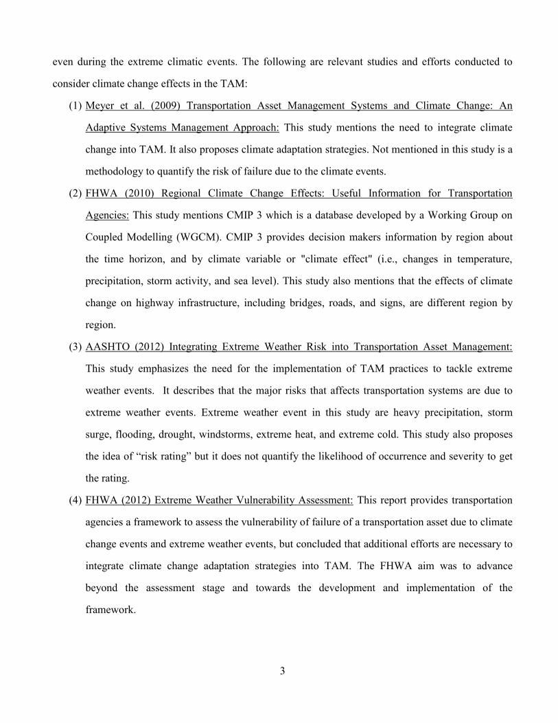
Figure 4: Observed Change in Annual Precipitation 1951-2010 (IPCC 2014)
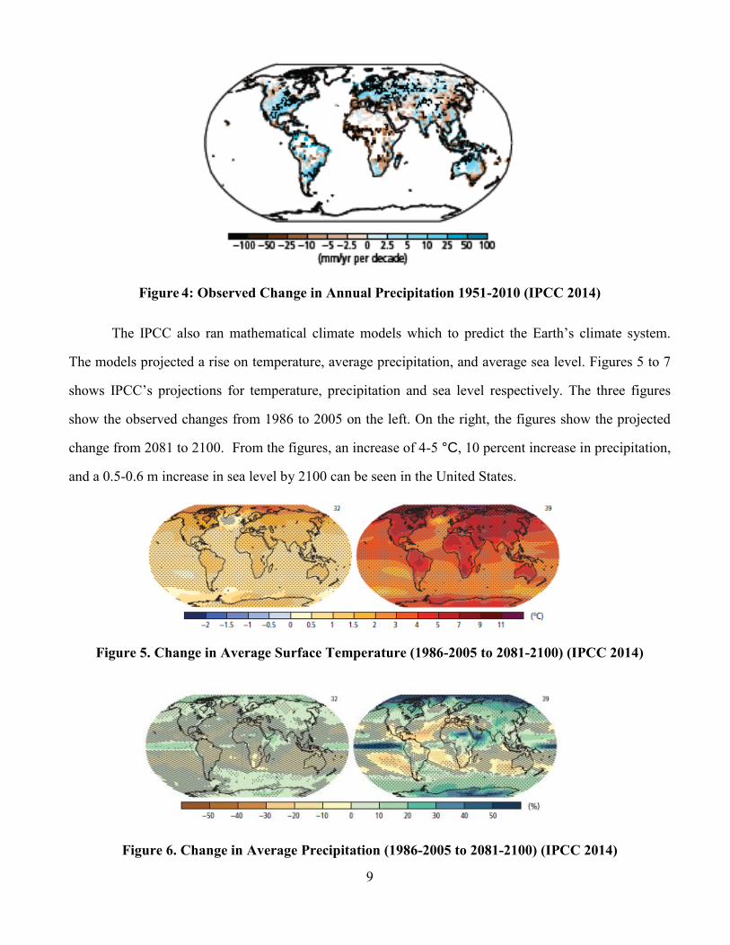
The IPCC also ran mathematical climate models which to predict the Earth’s climate system.
The models projected a rise on temperature, average precipitation, and average sea level. Figures 5 to 7
shows IPCC’s projections for temperature, precipitation and sea level respectively. The three figures
show the observed changes from 1986 to 2005 on the left. On the right, the figures show the projected
change from 2081 to 2100. From the figures, an increase of 4-5 °C, 10 percent increase in precipitation,
and a 0.5-0.6 m increase in sea level by 2100 can be seen in the United States.
Figure 5. Change in Average Surface Temperature (1986-2005 to 2081-2100) (IPCC 2014)
Figure 6. Change in Average Precipitation (1986-2005 to 2081-2100) (IPCC 2014)

10
Figure 7. Change in Average Sea Level (1986-2005 to 2081-2100) (IPCC 2014)
CAUSES OF CLIMATE CHANGE
According to NOAA, there are two reasons why the climate is changing. The first is that there is
a natural variability in the Earth. The natural variability relates to “interactions among the atmosphere,
ocean, and land, as well as changes in the amount of solar radiation reaching the earth” (NOAA 2007).
The second is that there is a human-induced change. The human induced change is caused by “the
increase in anthropogenic greenhouse gas concentrations” (NOAA 2007, IPCC 2014). Figure 8 shows a
relationship developed by IPCC for the anthropogenic change. From the figure, the mean temperature
increases as a function of cumulative total global carbon dioxide (CO2) emissions (IPCC 2014).
Figure 8: Cumulative Total Anthropogenic CO2emissions from 1870 (GtCO2) (IPCC 2014)
11
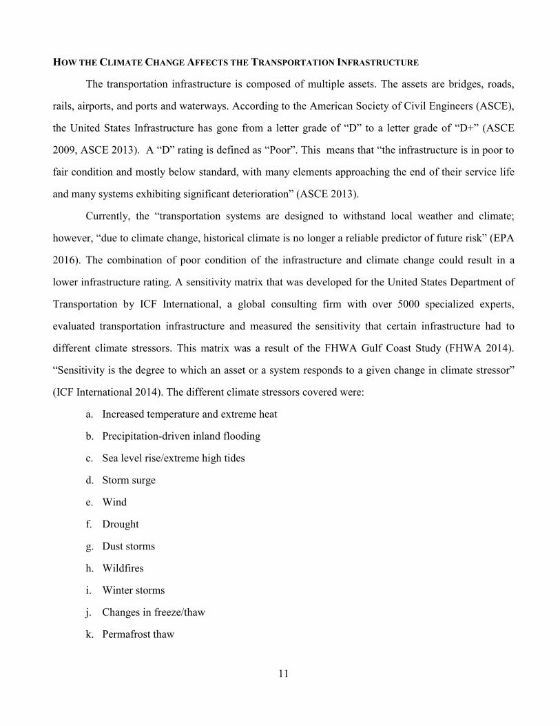
HOW THE CLIMATE CHANGE AFFECTS THE TRANSPORTATION INFRASTRUCTURE
The transportation infrastructure is composed of multiple assets. The assets are bridges, roads,
rails, airports, and ports and waterways. According to the American Society of Civil Engineers (ASCE),
the United States Infrastructure has gone from a letter grade of “D” to a letter grade of “D+” (ASCE
2009, ASCE 2013). A “D” rating is defined as “Poor”. This means that “the infrastructure is in poor to
fair condition and mostly below standard, with many elements approaching the end of their service life
and many systems exhibiting significant deterioration” (ASCE 2013).
Currently, the “transportation systems are designed to withstand local weather and climate;
however, “due to climate change, historical climate is no longer a reliable predictor of future risk” (EPA
2016). The combination of poor condition of the infrastructure and climate change could result in a
lower infrastructure rating. A sensitivity matrix that was developed for the United States Department of
Transportation by ICF International, a global consulting firm with over 5000 specialized experts,
evaluated transportation infrastructure and measured the sensitivity that certain infrastructure had to
different climate stressors. This matrix was a result of the FHWA Gulf Coast Study (FHWA 2014).
“Sensitivity is the degree to which an asset or a system responds to a given change in climate stressor”
(ICF International 2014). The different climate stressors covered were:
a. Increased temperature and extreme heat
b. Precipitation-driven inland flooding
c. Sea level rise/extreme high tides
d. Storm surge
e. Wind
f. Drought
g. Dust storms
h. Wildfires
i. Winter storms
j. Changes in freeze/thaw
k. Permafrost thaw
12
The following subsections describe how climate change affects bridges, roads and culverts, rails,
and ports and waterways. Also shown in the subsections are a number of performance measures used for
each type of asset.
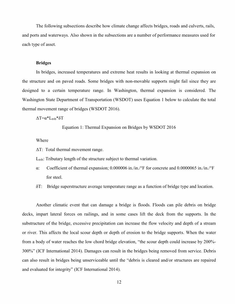
Bridges
In bridges, increased temperatures and extreme heat results in looking at thermal expansion on
the structure and on paved roads. Some bridges with non-movable supports might fail since they are
designed to a certain temperature range. In Washington, thermal expansion is considered. The
Washington State Department of Transportation (WSDOT) uses Equation 1 below to calculate the total
thermal movement range of bridges (WSDOT 2016).
ΔT=α*Ltrib*δT
Equation 1: Thermal Expansion on Bridges by WSDOT 2016
Where
ΔT: Total thermal movement range.
Ltrib: Tributary length of the structure subject to thermal variation.
α: Coefficient of thermal expansion; 0.000006 in./in./°F for concrete and 0.0000065 in./in./°F
for steel.
δT: Bridge superstructure average temperature range as a function of bridge type and location.
Another climatic event that can damage a bridge is floods. Floods can pile debris on bridge
decks, impart lateral forces on railings, and in some cases lift the deck from the supports. In the
substructure of the bridge, excessive precipitation can increase the flow velocity and depth of a stream
or river. This affects the local scour depth or depth of erosion to the bridge supports. When the water
from a body of water reaches the low chord bridge elevation, “the scour depth could increase by 200%-
300%” (ICF International 2014). Damages can result in the bridges being removed from service. Debris
can also result in bridges being unserviceable until the “debris is cleared and/or structures are repaired
and evaluated for integrity” (ICF International 2014).

13
Sea level rise combined with extreme storms can increase water levels near a bridge. Since
“many coastal bridges were designed to withstand erosion produced by storm surges having a 1% annual
change of occurrence, as sea level increases the statistics used to design these structures change.” A
higher baseline combined with a 50-year storm could “scour a bridge as severely as would the current
100- year storm surge.” Clearance under bridges is reduced due to higher baselines (ICF International
2014, Froehlich 2003).
Storms can create waves that stress the superstructure and the substructure of a bridge. ICF
International state that, “stress may damage or destroy the connection between the bridge’s
superstructure and substructure, leading to the bridge span to be shifted or even unseated completely.”
This shift can damage abutments, bent caps, and girders. During Hurricane Katrina, most bridges
damaged were near water (ICF International 2014, Padgett et al. 2009). Figure 9 displays a bridge along
the Texas coast thaw was damaged after Hurricane Ike.
Figure 9: State Highway 87 Rollover Pass Bridge Along the Texas Coast (Padgett et al. 2009)
Another climate stressor on bridges is wind. Winds can stress bridges with additional horizontal
forces and larger waves created by higher winds speeds. High winds can also lead to dust storms. The
dust storms can buildup material on the bridge deck, which will only retain water or moisture. This
moisture can be damaging to the bridge deck and structure (ICF International 2014). High winds can
also spread wildfires at a faster rate. “Infrastructure is at risk from both wildfires and any subsequent
debris-flow” (Cannon and DeGraff 2009). Post-wildfire debris flow can damage bridges by drag,
buoyancy, lateral impact or burial resulting in bridges displaced, lifted off their foundations, or damaged
from debris flow (ICF International, 2014, Cannon and DeGraff 2009).

14
Winter precipitation has also started to change. According to the National Research Council,
there is a “tendency for increasing winter precipitation and decreasing summer precipitation as global
temperatures increase” (NRC 2008). This increase in precipitation can saturate soils and as a result the
bridge is exposed to greater movement. Early start of seasonal warming can lead to shorter winters but
longer thaw seasons. This change in the freeze-thaw cycle can result in damage to bridge decks and
expansion in joints. Water begins seeping into the pavement on the bridge deck and accumulates in the
aggregate, resulting in the cement becoming susceptible to cracking. Over time, this cracking expands
upward until it reaches the road surface (ICF International 2014, NRC 2008). Figure 10 displays the
damage to concrete from freeze-thaw. This happens when an increase in the freeze-thaw cycles cracks
concrete and pavement surfaces (ICF International 2014).
Figure 10: Forms of Freezing and Thawing Damage to Concrete (West et al. 1999)
The impact of these climate change events on bridges can be monitored using performance
measures seen in Table 1 implemented by Departments of Transportation.

15
Table 1: Common Performance Measures for Bridges (Chang et al. 2017)
Performance Measure Description
National Bridge Inventory
General Condition Rating
0 (worst) – 9 (best) rating reported for deck, substructure,
and superstructure condition (and for culverts long enough to be
included in the NBI)
National Bridge Inventory
Structural Condition
Rating
Good, fair, or poor, calculated based on NBI condition and
appraisal ratings
National Bridge Inventory
(NBI) Structurally
Deficient (SD) /
Functionally Obsolete
(FO) Status
Calculated based on NBI data. A bridge that is Structurally
Deficient (SD) has a condition rating of 4 or less for either the deck,
superstructure, or substructure (or culvert in the case of NBI-length
culverts). Such bridges require rehabilitation, but are not
necessarily unsafe. A bridge that is FO fails to meet current
functional standards for deck geometry, load-carrying capacity,
clearances and/or approach roadway alignment.
Sufficiency Rating (SR) “0 (worst) –100 (best) scale based on four factors reflecting ability
to remain in service”: structural adequacy and safety, serviceability
and functional obsolescence, essentiality for public use, and special
reductions. Calculated based on NBI data.
Element condition Conditions for individual elements (e.g., the NBE) are summarized
by percent of element quantity by state, typically with four
condition states defined for an element.
Roads and Culverts
Constant high temperature can result in asphalt concrete pavement to soften resulting in rutting
and shoving. According to a report conducted for the Department of Transport in the United Kingdom,
“research has found that the majority of rutting in the asphalt surfacing occurs on a few days of the year,
when the temperature of the road surfacing exceeds 45 °C” (Willway et al. 2008). In July 2006, 80km of
damage to rural highways of Leicestershire, England occurred due to high temperatures (Willway et al.
2008)
Precipitation falling as rain rather than snow leads to immediate runoff. This increases the risk of
floods, landslides, slope failures, and consequent damage to roadways, especially rural roadways in the
winter and spring months. In paved roads, flooding can cause pavement and embankment failure and is
more prevalent when the water is high enough to flow over the roadway surface. Over time,
precipitation can also worsen existing pavement damage like cracking. During heavy precipitation
events, rain can leak in under the pavement due to the cracks and damage the subgrade. The subgrade is

16
very sensitive to moisture levels (NRC 2008, ICF International 2014). Unpaved roads and culverts can
also be affected by heavy precipitation. In culverts, heavy precipitation can cause debris accumulation,
sedimentation, erosion, scour, piping, and conduit structural damage. All these can result in flooding
(ICF International 2014).
Roadways can get damaged by the storm surge from hurricanes like Hurricane Sandy and many
other hurricanes. Hurricane Sandy caused massive flooding of roads and tunnels in New York and New
Jersey Roadways and tunnels in New York City. The flooding included the Brooklyn-Battery, Holland,
and Midtown Tunnels and the Battery Park underpass (Kaufman et al. 2012 and ICF International 2014).
Figure 11 displays the flooding resulting from Hurricane Sandy on New York City.
Figure 11: Flooding in New York as a Result of Hurricane Sandy (Kaufman et al. 2012)
High winds usually accompany storms. Although winds do not directly damage the road, they
can severely disrupt road traffic and other service activities by damaging trees, buildings, and other
structures to disrupt activities (ICF International 2014). In New York, Hurricane Sandy’s strong winds
knocked down trees resulting in power outages to millions (Kaufman et al. 2012). The debris can also

17
end up in the storm water drainage. This can result in flooding impacts to the surrounding area (ICF
International 2014).
Drought can also damage pavements by creating cracking and splitting. In 2011, droughts in
Texas led to asphalt splitting and cracking (ICF International 2014 and Auber 2011). During a drought,
the clayey soil will shrink and if the movement is great, the asphalt will crack as a result. This is due to
the fact that clayey soils are susceptible to shrinking and swelling. Figure 12 below shows the cracks
that formed in Fort Worth as a result of a drought.
Figure 12: Cracks in Pavement Due to Drought in Texas (Auber 2011)
Wildfires are extremely dangerous to human life and roadways. The wildfire’s high heat can
ignite road surfaces and soften the asphalt, which can result in rutting. After a wildfire, hillslopes of
vegetation and soil properties change resulting in the change of watershed hydrology and the sediment-
transport processes (ICF International 2014). A rainstorm after a wildfire can increase runoff that can
erode soil, rock, ash, and vegetative debris from the hillslopes and damage roads and culverts (Verdin et
al. 2012). The debris-flow can result in blocking drainage ways, and damage structures (ICF
International 2014). Figure 13 displays a landslide that covered a roadway in Arizona after the South
Canyon wildfire.
18
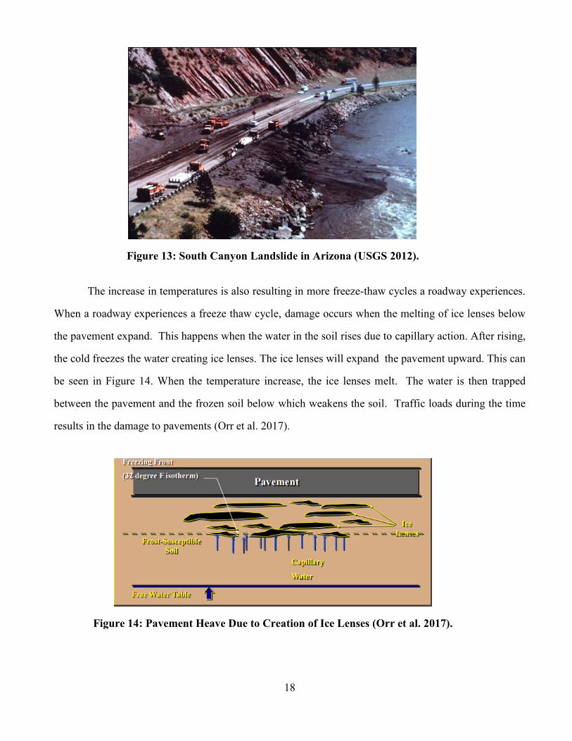
Figure 13: South Canyon Landslide in Arizona (USGS 2012).
The increase in temperatures is also resulting in more freeze-thaw cycles a roadway experiences.
When a roadway experiences a freeze thaw cycle, damage occurs when the melting of ice lenses below
the pavement expand. This happens when the water in the soil rises due to capillary action. After rising,
the cold freezes the water creating ice lenses. The ice lenses will expand the pavement upward. This can
be seen in Figure 14. When the temperature increase, the ice lenses melt. The water is then trapped
between the pavement and the frozen soil below which weakens the soil. Traffic loads during the time
results in the damage to pavements (Orr et al. 2017).
Figure 14: Pavement Heave Due to Creation of Ice Lenses (Orr et al. 2017).

19
Figure 15 shows variation of the subgrade resilient modulus over a freeze-thaw cycle. This figure
shows that, during freeze periods, the soil will gain more strength. During thaw periods, the strength is
lower than the normal strength before returning to normal.
Figure 15: Subgrade Resilient Modulus Seasonal Variation (Huang 1993)
Tables 2 and 3 summarize the performance measures implemented by Departments of
Transportation of pavements and culverts respectively that can be used to monitor the impact of these
climate change events.
Table 2: Common Performance Measures for Pavements (Chang et al. 2017)
Performance Measure Description
International Roughness
Index (IRI)
IRI is “an index computed from a longitudinal profile measurement
using a quarter-car simulation at a simulation speed of 50 mph (80
km/h)”. It is related to pavement smoothness that affects the riding
comfort when traveling. DOTs are required to report the IRI to
FHWA every year since 1993 as part of the HPMS data submittal.
Pavement Condition Index
(PCI)
PCI is “a numerical rating of the pavement condition that ranges
from 0 to 100 with 0 being the worst possible condition and 100
being the best possible condition”

20
Table 2: Common Performance Measures for Pavements (Chang et al. 2017) (cont’d)
Performance Measure Description
Present Serviceability
Index (PSI)
PSI measures the pavement “ability to serve the type of traffic
which use the facility”. It ranges from 0 (collapsed road) to 5
(perfect road). It is obtained from a mathematical combination of
certain physical measurements (e.g., rut depth, cracking, slope
variance). This performance measure is related to the functional
pavement capacity to provide a smooth ride.
Present Serviceability
Rating (PSR)
PSR is “a mean rating of the serviceability of a pavement (traveled
surface) established by a rating panel under controlled conditions.
The accepted PSR scale for highways is 0 to 5, with 5 being
excellent”. PSR is an indicator of the riding comfort of the users
when traveling the roadway section.
Skid Number (SN)
or
Friction Number (FN)
The Friction Number (FN) or Skid Number (SN) is locked-wheel
testing device, represents the average coefficient of friction
measured across a test interval. The reporting SN values range from
0 to 100 (0 represents no friction and 100 complete friction). This
performance measure is related to safety regulations. The National
Highway Safety Act of 1996 mandates to correct excessive
slipperiness.
International Friction
Index (IFI)
In the early 1990s, the World Road Association (PIARC) developed
the International Friction Index (IFI) in order to measure friction on
roads. The IFI is composed of two numbers, the friction number
(F60) and the speed number (Sp). The F60 represents the friction
value of a pavement at a slip speed of 37 mph (60 km/h), and the Sp
is the variation of speed and friction at speeds different than 37 mph
(60 km/h).
Cracking There are different types of cracks including longitudinal,
transverse, block or map, and edge. Longitudinal cracks are
“predominantly parallel to the direction of traffic.” Transverse
cracks are “predominantly perpendicular to the direction of traffic.”
Map or block cracks are “interconnected cracks that extend only
into the upper portion of the slab.” Edge cracks are “crescent-
shaped cracks or fairly continuous cracks that are located within 2 ft
(0.6 m) of the pavement edge”
Rutting Rutting is “a surface depression in the wheel paths,” which “stems
from a permanent deformation in any of the pavement layers or
subgrades, usually caused by consolidated or lateral movement of
the materials due to traffic load”. Rut depth is “the maximum
measured perpendicular distance between the bottom surface of the
straightedge and the contact area of the gauge with the pavement
surface at a specific location”.
Faulting Faulting is “difference in elevation across a joint or crack”. It is a
common distress in jointed plain concrete pavements.
21
Table 2: Common Performance Measures for Pavements (Chang et al. 2017) (cont’d)
Performance Measure Description
Structural Number (SN) The SN is a function of the layers’ thicknesses, structural material
coefficients, and drainage coefficients. It is a number represents the
pavement capacity to withstand traffic loads.
Remaining Service Life
(RSL)
RSL is defined as “the time until the next rehabilitation or
reconstruction event”, also as the time until a condition index (or
distress) trigger value is reached”
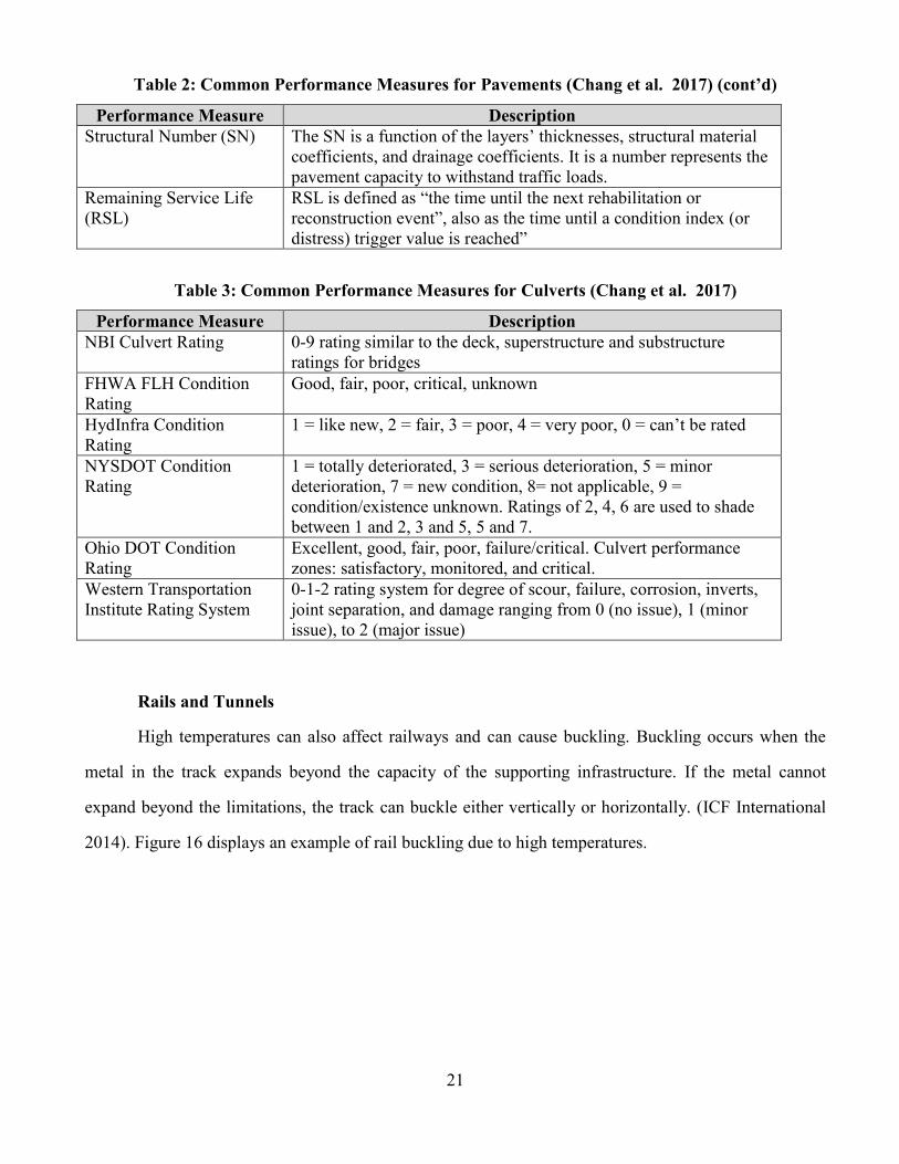
Table 3: Common Performance Measures for Culverts (Chang et al. 2017)
Performance Measure Description
NBI Culvert Rating 0-9 rating similar to the deck, superstructure and substructure
ratings for bridges
FHWA FLH Condition
Rating
Good, fair, poor, critical, unknown
HydInfra Condition
Rating
1 = like new, 2 = fair, 3 = poor, 4 = very poor, 0 = can’t be rated
NYSDOT Condition
Rating
1 = totally deteriorated, 3 = serious deterioration, 5 = minor
deterioration, 7 = new condition, 8= not applicable, 9 =
condition/existence unknown. Ratings of 2, 4, 6 are used to shade
between 1 and 2, 3 and 5, 5 and 7.
Ohio DOT Condition
Rating
Excellent, good, fair, poor, failure/critical. Culvert performance
zones: satisfactory, monitored, and critical.
Western Transportation
Institute Rating System
0-1-2 rating system for degree of scour, failure, corrosion, inverts,
joint separation, and damage ranging from 0 (no issue), 1 (minor
issue), to 2 (major issue)
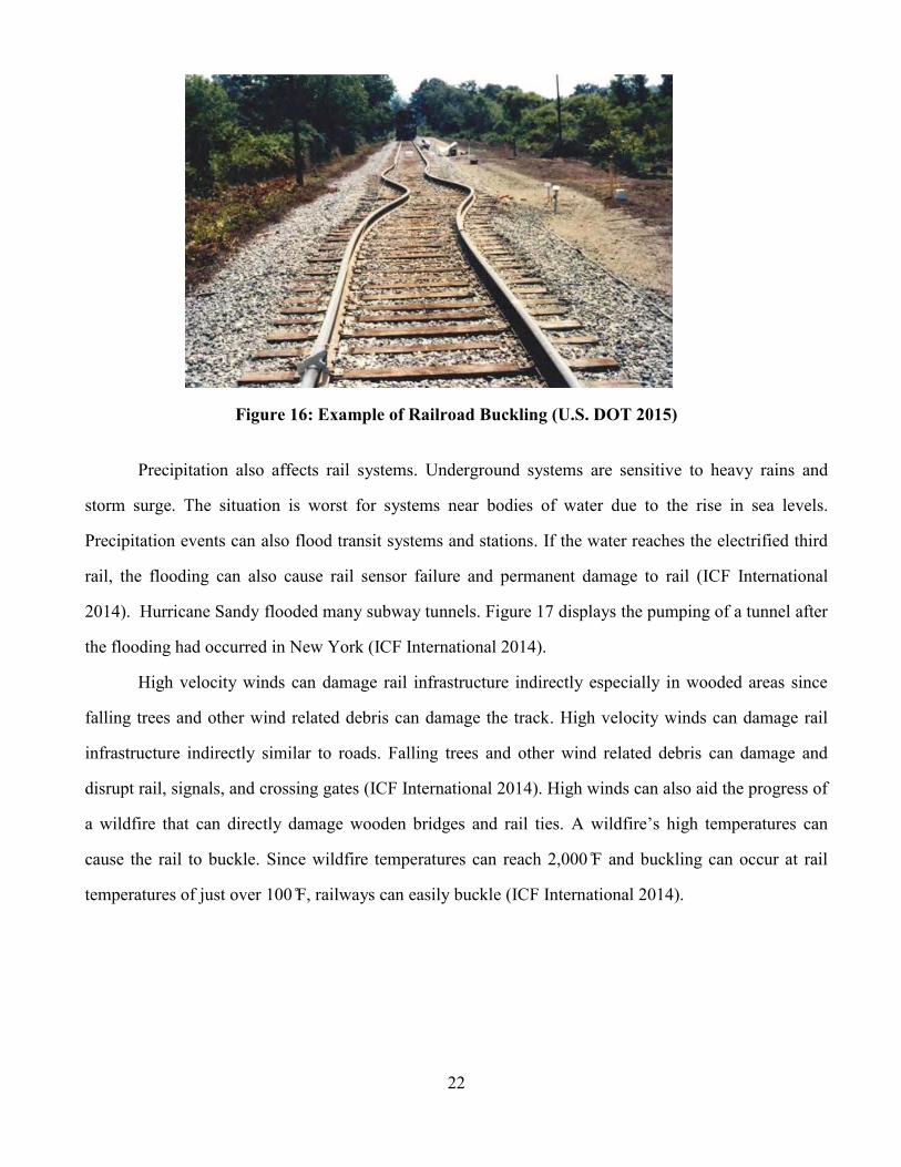
Rails and Tunnels
High temperatures can also affect railways and can cause buckling. Buckling occurs when the
metal in the track expands beyond the capacity of the supporting infrastructure. If the metal cannot
expand beyond the limitations, the track can buckle either vertically or horizontally. (ICF International
2014). Figure 16 displays an example of rail buckling due to high temperatures.
22
Figure 16: Example of Railroad Buckling (U.S. DOT 2015)
Precipitation also affects rail systems. Underground systems are sensitive to heavy rains and
storm surge. The situation is worst for systems near bodies of water due to the rise in sea levels.
Precipitation events can also flood transit systems and stations. If the water reaches the electrified third
rail, the flooding can also cause rail sensor failure and permanent damage to rail (ICF International
2014). Hurricane Sandy flooded many subway tunnels. Figure 17 displays the pumping of a tunnel after
the flooding had occurred in New York (ICF International 2014).
High velocity winds can damage rail infrastructure indirectly especially in wooded areas since
falling trees and other wind related debris can damage the track. High velocity winds can damage rail
infrastructure indirectly similar to roads. Falling trees and other wind related debris can damage and
disrupt rail, signals, and crossing gates (ICF International 2014). High winds can also aid the progress of
a wildfire that can directly damage wooden bridges and rail ties. A wildfire’s high temperatures can
cause the rail to buckle. Since wildfire temperatures can reach 2,000 ̊F and buckling can occur at rail
temperatures of just over 100 ̊F, railways can easily buckle (ICF International 2014).

23
Figure 17: Flooding of a Subway Tunnel after Hurricane Sandy in New York City
(Kaufman et al. 2012)
The rail infrastructure is also affected by freeze-thaw cycles. Similar to roads, the water
expansion from the freeze-thaw cycles can cause damage to railways due to the changes in strength of
the soil foundation. Table 4 summarize the performance measures implemented by Departments of
Transportation of rails and tunnels that can be used to monitor the impact of these climate change
events.
Table 4: Common Performance Measures for Rails and Tunnels (Chang et al. 2017)
Performance Measure Description
Track Stiffness The track stiffness is used to determine effectiveness of the rail
embankment. The ballast should transfer the vertical load, maintain
the track in a fixed position, provide elasticity of track and
absorption of energy, ensure drainage of water, and set and level the
surface of the track (Stenstrom et al. 2012)
Q Index The Q index is a parameter over a 200 m long track segment. The Q
index ranges from 10 to 0. The larger the Q index, the better the
track (Liu et al. 2015).
P Index P Index. P index is adopted by Japanese railroads and is the ratio of
the number of sampling points whose quality parameter
measurements fall outside ±3 mm to the number of all sampling
points in a track segment. There are two lengths of track segments
over which P index is applied, 100 m and 500 m. The larger the P
index, the worse the track segment in some quality aspect (Liu et al.
2015).

24
Table 4: Common Performance Measures for Rails and Tunnels (Chang et al. 2017) (cont’d)
Performance Measure Description
Track Quality Index (TQI) The TQI is a 2nd order polynomial equation of the standard
deviation 𝜎𝑖 of measurement values for a quality parameter over a
track segment to assess its partial quality The overall quality
assessment is achieved by averaging six partial quality indices for
gauge, cross level, left (right) surface, and left (right) alignment. A
larger track quality index implies the track segment has a better
quality (Liu et al. 2015).
Track Geometry Index
(TGI)
Track geometry index uses the measurement value space curve
length for a quality parameter over a track segment to quantify the
quality of the track segment. A larger TGI𝑖 indicates that the track
segment has a worse quality (Liu et al. 2015).
Buckling This occurs when the metal in the track expands beyond the
capacity of the supporting infrastructure. If the metal cannot expand
beyond the constraints the track will buckle either vertically or
horizontally (ICF International 2014).
Level of Service Rating A way to quantify how well a preservation action improves the
service level is to simply provide a rating 1 to 100 as a qualitative
assessment of performance of a tunnel (Allen et al. 2015).
Level of Service Score An average rated level of service from 1 to 100 for tunnels with
weighted individual ratings scaled from 1 to 5 on six tunnel level of
service categories including Reliability, Safety, Security,
Preservation, Quality of Service, and Environment (Allen et al.
2015).
Risk of Urgency (RBU)
Score
The RBU, on a scale of 0 to 100, is calculated based on a user-input
rating of 0 to 10 for urgency, where 10 indicates an action that is
very urgently required and 0 indicates an action that would be
beneficial, but is not necessarily urgent at the time of the analysis
(Allen et al. 2015).
Ports and Waterways
Ports and waterways are a major part of the transportation network and can also be affected by
climate change. They are essential for international and domestic trade. According to ICF International,
“Higher sea levels can increase the risk of chronic flooding” (ICF International 2014).As for flooding,
the flooding can damage channels, damage piers, wharves, and berths. “While erosion can weaken
supports, most channels and waterways are built to withstand erosion. However, increased erosion rates
may not be adequately planned for and could this impact port support structures” (ICF International,
2014).
25
High winds and changes in the freeze-thaw cycle can also affect ports and waterways. “Highway
signage has to withstand winds of 125 mph but varies by location, but if equipment (like signage) falls
into the channel, it has to be cleaned up before shipping can resume” (ICF International 2014). As
discussed in previous section, freeze-thaw can undermine the foundations of infrastructure through the
weakening of soil.
One performance measure for ports and waterway was found. The Physical Condition Rating of
Critical Coastal Navigation Infrastructure rates the ports and waterway’s infrastructure on a scale of A to
F (significant damage to completely degraded) (CMTS 2015).
ECONOMIC IMPACT
Economic losses for a region can be a result of extreme climatic events. This can result due to
the unbudgeted expenses that an agency will have to invest to return the transportation system to a
working condition. This can be seen in a study conducted to report the bridge damage and repair costs
from Hurricane Katrina. In damages only to bridges, the hurricane cost an estimated $8.15 million to
Alabama, $52.23 million to Louisiana, and $569 million to Mississippi (Padgett et al. 2008).
One way to determine the economic impact is described in NCHRP Report 750. It describes a
benefit cost methodology to evaluate climate change adaptation strategies. The methodology described
in this report consists of eight steps. The steps are identify the highest risk infrastructure, estimate future
operations and maintenance costs, estimate the agency costs of asset failure, estimate the user cost of
asset failure, estimate likelihood of asset failure, calculate agency benefits of the strategy, calculate the
user benefits of the strategy, and evaluate the results (NCHRP 2013).
TRANSPORTATION INFRASTRUCTURE LAWS
Presently, there are two main national laws on transportation infrastructure. They are the Moving
Ahead for Progress in the 21st Century (MAP-21) and Fixing America’s Surface Transportation (FAST)
Act. The first law, MAP-21, was signed on July 17, 2012 and established a performance and outcome
based program. MAP-21 was extended until May 2015. “The objective of this performance and outcome

26
based program is for States to invest resources in projects that collectively will make progress toward
the achievement of the national goals” (U.S. DOT 2013). The seven national goals are shown in Table 5.
Table 5: MAP-21 National Goals (U.S. DOT 2013)
Goal Area National Goal
Safety To achieve a significant reduction in traffic fatalities and serious
injuries on all public roads
Infrastructure Condition To maintain the highway infrastructure asset system in a state of
good repair
Congestion Reduction To achieve a significant reduction in congestion on the National
Highway System
System Reliability To improve the efficiency of the surface transportation system
Freight Movement and
Economic Vitality
To improve the national freight network, strengthen the ability of
rural communities to access national and international trade
markets, and support regional economic development
Environmental
Sustainability
To enhance the performance of the transportation system while
protecting and enhancing the natural environment
Reduced Project Delivery
Delays
To reduce project costs, promote jobs and the economy, and
expedite the movement of people and goods by accelerating project
completion through eliminating delays in the project development
and delivery process, including reducing regulatory burdens and
improving agencies’ work practices
The FAST Act is a “five-year legislation to improve the Nation’s surface transportation
infrastructure, including our roads, bridges, transit systems, and rail transportation network. The bill
reforms and strengthens transportation programs, refocuses on national priorities, provides long-term
certainty and more flexibility for states and local governments, streamlines project approval processes,
and maintains a strong commitment to safety” (House Transportation and Infrastructure Committee
2015). The bill enacted in December 2015 and extended until fiscal year 2020.
In October 24, 2016, the Federal Highway Administration (FHWA) released a rule for asset
management plan. The plan stated that “a state shall develop a risk-based asset management plan that
describes how the NHS will be managed to achieve system performance effectiveness and State DOT
targets for asset condition, while managing the risks, in a financially responsible manner, at a minimum
practicable cost over the life cycle of its assets” (FHWA 2016b). In the next sections, transportation
asset management and risk management practices are discussed.

27
TRANSPORTATION ASSET MANAGEMENT
Transportation Asset Management (TAM) “is a strategic and systematic process of operating,
maintaining, upgrading, and expanding physical assets effectively throughout their lifecycle. It focuses
on business and engineering practices for resource allocation and utilization, with the objective of better
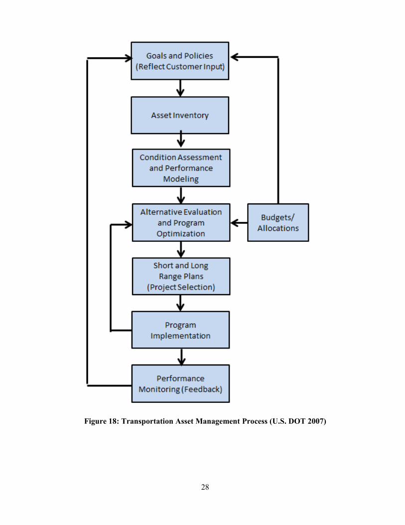
decision making based upon quality information and well defined objectives” (U.S. DOT 2007). TAM is
comprised of seven components and is displayed in Figure 18. They are goals and policies, asset
inventory, condition assessment and performance modeling, alternatives evaluation and program
optimization, short and long range plans, program implementation, and performance monitoring.
TAM begins by first identifying goals and policies for maintenance, repair and rehabilitation.
Goals and policies need to be clearly defined having clear performance measures to set targets to be able
to measure progress for the transportation infrastructure. The next step in the system is asset inventory.
An agency, to be successful, must keep updated records of the asset inventory to provide reliable data
for all the assets. After the asset inventory, TAM requires performing periodical condition assessments
of all the assets in the inventory. It also requires performance models to forecast the future condition.
Alternatives for maintenance and rehabilitation programs are analyzed next. The programs are used to
determine the best course of action in terms of performance and resource allocation. The next step is the
short- and long- range plans, which come as a result of the evaluations. Following the plans, program
implementation begins to preserve the assets in the most cost-effective manner. The final step in the
TAM is to monitor the asset performance and check if the assets operates as expected. This checks to
see if the goals are being accomplished (Meyer et al. 2009).
28
Figure 18: Transportation Asset Management Process (U.S. DOT 2007)

29
Chapter 3: Development of the Framework for Modeling Climate Change in TAM
FRAMEWORK FOR CLIMATE CHANGE MODELING IN TAM
As climate change continues to change weather patterns, the resilience of transportation assets
must be considered (U.S. DOT n.d. a). Although there are a number of definitions for resiliency, in this
thesis resilience in infrastructure is defined as “the ability for an infrastructure asset to maintain a level
of robustness during or after an extreme event and to return itself to a desired level of performance
within the shortest possible time to minimize the impact on the community” (Minaie 2016). A highly
resilient asset continues to function properly under extreme circumstances. As a result, TAM practices
should consider the impact of climate change on the resilience of transportation infrastructure.
If an asset is not resilient, an extreme climatic event will have costly impacts to humans and
budgets (NCHRP 2014). AASHTO (2012) and FHWA (2012) offered deterministic methods like low,
medium, or high levels of risk to integrate climate change into TAM practices. The AASHTO approach
defines consequence categories: “insignificant, minor, significant, major, and catastrophic”; and the
likelihood of occurrence for a climate event: “frequent, common, seldom, rare, and very rare”
(AASHTO 2012). As for the FHWA, it defines a 1 to 10 scale for the consequence (least critical to
critical), and a 1 to 10 impact parameter (reduced capacity to complete failure). Although both reports
show the need for integrating climate change into TAM, their methodologies to determine the impact are
based on expert opinion collected through a questionnaire.
Figure 19 displays the project management process for individual assets. The first step in this
process begins with the monitoring of the current performance measures to develop the project plans.
After that, the forecast of the asset performance is conducted for the actions considered in the project
plans. Next, depending on available funding, the project is then designed and delivered. As a result of
this process, an improved performance is expected for this asset while it is being monitored over time.
The project management process must be part of the overall TAM and should consider climate
mitigation practices for the entire transportation network.

30
Figure 19: Project Management Process (AASHTO 2011)
The framework for climate change modeling in TAM is presented in Figure 20. This was
developed using the Transportation Asset Management Process and the Project Management Process
described previously. The framework for climate change modeling in TAM was developed for the entire
transportation network and consists of eight main steps.

31
Figure 20: Framework to Integrate Climate Change Impact Analysis into TAM Practices
Step 1: Goals and Policies
The framework begins with an agency defining the goals and policies. Goals are the “results to
be achieved” while policies are the “intentions and direction of an organization” (ISO 2014). Without
clearly identifiable goals, a lack of guidance and direction will exist. Goals and policies help in the
evaluation of assets and facilitate planning. In this step, an agency must also define the desired level of
service, life cycle, or performance of an asset. The development of performance measures can useful to
gage the asset’s conditions and track progress towards achieving the goals. Climate change performance

32
measures will need to be selected in this step. This will facilitate and track progress of the goals and
policies. More specific performance measures are required to properly evaluate the effects of climate
change. An example of a performance measure is the number of bridges in high risk of climate change
impact.
Step 2: Asset Inventory
According to the FHWA, “a major component of an effective Asset Management program is the
existence of an inventory of infrastructure assets by type and their condition” (FHWA 2017). The
inventory should include the following:
Type of asset
Dimensions
Location
Any other pertinent information to identify the asset managed by the agency
“Transportation infrastructure assets are the physical elements, such as pavements, bridges,
culverts, signs, pavement markings, and other roadway and roadside features that comprise the whole
highway infrastructure network, from right-of-way line to right-of-way line” (FHWA 2017). Apart from
collecting asset information, climate data collection is important in the region. The National Oceanic and
Atmospheric Administration (NOAA) created an online database with climate change tools, as see in
Table 6, that can help to analyze climate change scenarios (NOAA 2017).
Table 6: NOAA Climate Change Tools (NOAA 2017)
Tool Name Climate Data Description
The Climate
Explorer Precipitation
Temperature
This tool evaluates precipitation and temperature data
and projections by zip, city or state. This tool contains
historical data and projections.
https://toolkit.climate.gov/climate-explorer2/
Global Climate
Change Viewer Precipitation
Temperature
This tool is used to visualize future temperature and
precipitation changes by country. It also contains
histograms and monthly temperature projections.
http://regclim.coas.oregonstate.edu/gccv/
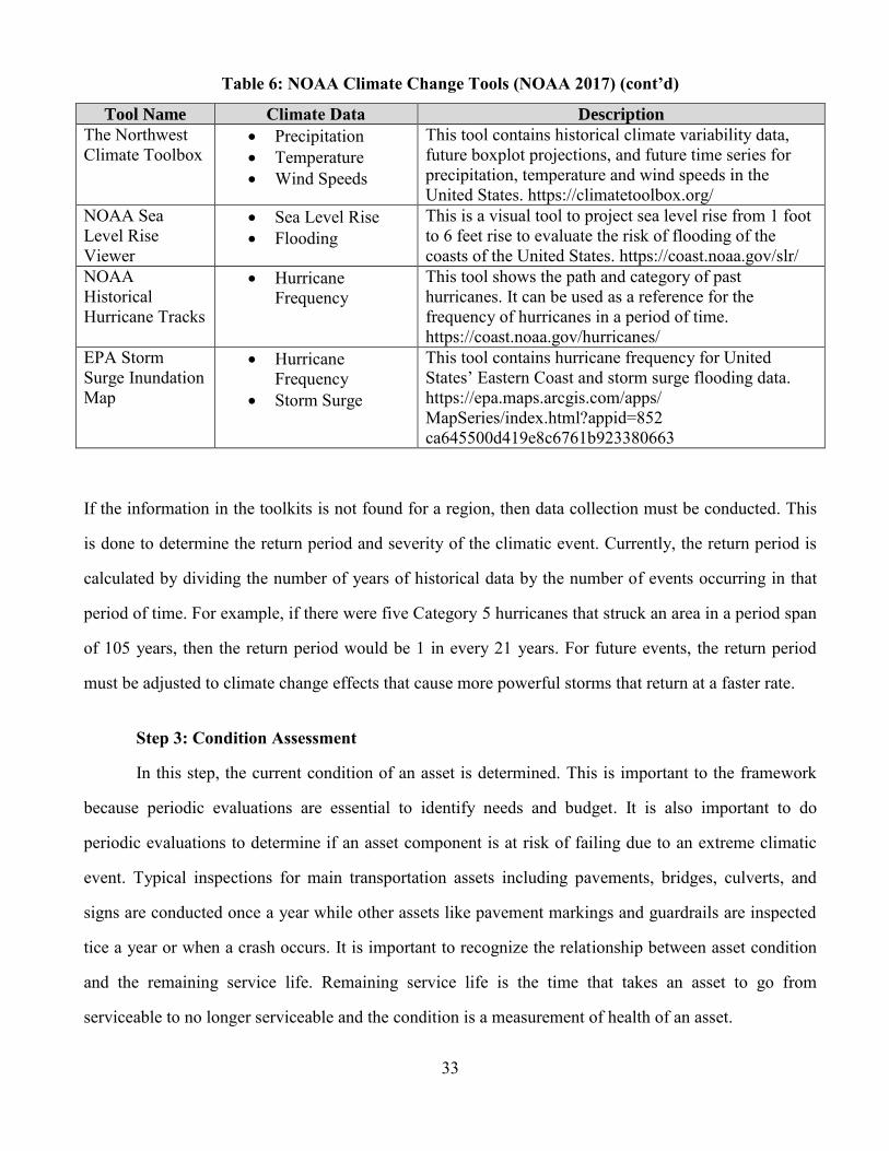
33
Table 6: NOAA Climate Change Tools (NOAA 2017) (cont’d)
Tool Name Climate Data Description
The Northwest
Climate Toolbox Precipitation
Temperature
Wind Speeds
This tool contains historical climate variability data,
future boxplot projections, and future time series for
precipitation, temperature and wind speeds in the
United States. https://climatetoolbox.org/
NOAA Sea
Level Rise
Viewer
Sea Level Rise
Flooding
This is a visual tool to project sea level rise from 1 foot
to 6 feet rise to evaluate the risk of flooding of the
coasts of the United States. https://coast.noaa.gov/slr/
NOAA
Historical
Hurricane Tracks
Hurricane
Frequency
This tool shows the path and category of past
hurricanes. It can be used as a reference for the
frequency of hurricanes in a period of time.
https://coast.noaa.gov/hurricanes/
EPA Storm
Surge Inundation
Map
Hurricane
Frequency
Storm Surge
This tool contains hurricane frequency for United
States’ Eastern Coast and storm surge flooding data.
https://epa.maps.arcgis.com/apps/
MapSeries/index.html?appid=852
ca645500d419e8c6761b923380663
If the information in the toolkits is not found for a region, then data collection must be conducted. This
is done to determine the return period and severity of the climatic event. Currently, the return period is
calculated by dividing the number of years of historical data by the number of events occurring in that
period of time. For example, if there were five Category 5 hurricanes that struck an area in a period span
of 105 years, then the return period would be 1 in every 21 years. For future events, the return period
must be adjusted to climate change effects that cause more powerful storms that return at a faster rate.
Step 3: Condition Assessment
In this step, the current condition of an asset is determined. This is important to the framework
because periodic evaluations are essential to identify needs and budget. It is also important to do
periodic evaluations to determine if an asset component is at risk of failing due to an extreme climatic
event. Typical inspections for main transportation assets including pavements, bridges, culverts, and
signs are conducted once a year while other assets like pavement markings and guardrails are inspected
tice a year or when a crash occurs. It is important to recognize the relationship between asset condition
and the remaining service life. Remaining service life is the time that takes an asset to go from
serviceable to no longer serviceable and the condition is a measurement of health of an asset.
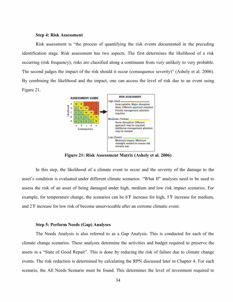
34
Step 4: Risk Assessment
Risk assessment is “the process of quantifying the risk events documented in the preceding
identification stage. Risk assessment has two aspects. The first determines the likelihood of a risk
occurring (risk frequency); risks are classified along a continuum from very unlikely to very probable.
The second judges the impact of the risk should it occur (consequence severity)” (Ashely et al. 2006).
By combining the likelihood and the impact, one can access the level of risk due to an event using
Figure 21.
Figure 21: Risk Assessment Matrix (Ashely et al. 2006)
In this step, the likelihood of a climate event to occur and the severity of the damage to the
asset’s condition is evaluated under different climate scenarios. “What If” analyses need to be used to
assess the risk of an asset of being damaged under high, medium and low risk impact scenarios. For
example, for temperature change, the scenarios can be 8 ̊F increase for high, 5 ̊F increase for medium,
and 2 ̊F increase for low risk of become unserviceable after an extreme climatic event.
Step 5: Perform Needs (Gap) Analyses
The Needs Analysis is also referred to as a Gap Analysis. This is conducted for each of the
climate change scenarios. These analyses determine the activities and budget required to preserve the
assets in a “State of Good Repair”. This is done by reducing the risk of failure due to climate change
events. The risk reduction is determined by calculating the RPN discussed later in Chapter 4. For each
scenario, the All Needs Scenario must be found. This determines the level of investment required to

35
reduce the risk to an acceptable level. Figure 22 shows the risk management process. In order to reduce
the risk, the whole process must be considered.
Figure 22: Risk Management Process (Ashley et al. 2006)
The FHWA proposed this risk management process for individual projects, and it can also be
extended to all the assets in the transportation network. The first step is to “identify and categorize risks
that could affect the project and document these risks.” The second step is to “Assess/Analyze” the risk
for the assets. In this step, “the process of quantifying the risk events documented in the preceding
identification stage.” In the risk assessment process, there are two main aspects to analyze. They are the
likelihood of the risk to occur as “very unlikely to very probable” and the consequences in the asset
condition. The third step is to “Mitigate and Plan” with the aim “to explore risk response strategies for
the high-risk items identified in the qualitative and quantitative risk analysis” (Ashley 2006)
According to Ashley, there are four alternatives to manage risk. Avoidance is the elimination of
risk and transference is the transfer of financial responsibility of risk by contracting out management
activities. Mitigation seeks to reduce the risk or impact of the event while acceptance is the agreeing of
risk as they occur. In the fourth step, “Allocate”, risk management activities are assigned to an
individual or department responsible for addressing the risk. The fifth step is to “Monitor and Control”
the risk management activities. The objective is to “systematically track the identified risks, identify any
new risks, effectively manage the contingency reserve, and capture lessons learned for future risk
assessment and allocation efforts.” Monitor and control “must continue for the life of the project because

36
risks are dynamic. The list of risks and associated risk management strategies will likely change as the
project matures and new risks develop or anticipated risks disappear” (Ashley 2006).
Climate mitigation involves actions to reduce the consequences of climate change by focusing on
the source (e.g. greenhouse gases). Climate adaptation seeks to be prepared to climate change threats by
creating costal building defenses, modifying existing assets to be more resilient, and other actions. Table
7 summarizes some climate mitigation and adaptation strategies. Some of the climate adaptation
strategies were fostered by the United Nations (2013) and (U.S. DOT n.d. b).
Table 7: Climate Mitigation and Adaptation Strategies
Climate Change
Stressor
Transportation
Asset Affected Mitigation and Adaptation Strategies
Increased Temperature Rail lines
Roads
Use of continuous welded rail lines to
prevent buckling.
Paint tracks or roads white to reduce the
heat.
Increased
Precipitation/Flooding Rail lines
Tunnels
Roads
Culverts and
Drainage Systems
Protect critical evacuation routes.
Continuously monitor water flows.
Riprap development in bridge piers and
abutments.
Flood plain restrictions.
Increase in culvert capacity.
Installation of flood gates.
Sea Level Rise and
Storm Surge Rail lines
Tunnels
Bridges
Roads
Increase elevation of bridges, rail lines,
roadways.
Build a sheetpile wall and cap.
Relocated sections of roadways to less
vulnerable to flooding.
Create a living shoreline (e.g. mashes)
Addition of drainage canals near coastal
roads.
Increase protection of high value roads
with levees, dikes, and seawalls.
Strengthen and increase height of
levees, seawalls, and dikes.
Increase pumping capacity of tunnels.
Restrict vulnerable areas.
Check bridge designs to assure decks
are tied to substructure.

37
Table 7: Climate Mitigation and Adaptation Strategies (cont’d)
Climate Change
Stressor
Transportation
Asset Affected Mitigation and Adaptation Strategies
Increase in Frequency
of Strong Storms Rail lines
Bridges
Roads
Increase levee height and strength.
Increase drainage capacity.
Return some coastal areas to nature.
Protect critical evacuation routes.
Decentralize systems.
These mitigation and adaptation strategies can be implemented in any region to reduce the risk of
asset failure from climate change. The strategies can help agencies think about actions to reduce risk, but
the driving factor for their implementation depends on the budget of each agency. Some mitigation and
adaptation strategies are expensive. An example of an expensive strategy is increasing the elevation of a
bridge or relocating sections of roadways. Other strategies, such as painting white tracks, are not as
expensive.
Step 6: Conduct Scenarios Analyses
In this step, scenario analyses can be formulated for different budget levels, climatic events, and
risk tolerance. An example for budget scenario analyses can be conducted for 75%, 50%, and 25% of the
all needs budget. For climatic event scenarios, the analysis may consider specific climatic events such as
hurricanes, flooding at different levels of magnitude. For risk tolerance, an agency may favor to invest
more funds to preserve the transportation infrastructure at a minimum risk of failure or accept moderate
risk to reduce the investments in the short-term. With these results of the scenarios analysis, an agency
can prioritize their available resources by focusing on risk reduction to preserve the transportation
infrastructure in a “State of Good Repair”.
Step 7: Asset Management Report and Risk Assessment
Here, a risk assessment section is included in the asset management reports. This section
describes the threats and actions to improve the resilience of the asset by reducing the risk of damage
where the actions are grouped into project categories and prioritized by asset groups. The driving factors
of these projects are the available budget and risk tolerance in the short and long-term. If there is

38
residual risk with a course of action already defined, the agency has to specify how to improve the
action or manage the risk. This information should assist the agencies with the implementation of the
asset management program to enhance the resiliency of the entire transportation infrastructure network
under extreme events.
Step 8: Asset Management Program to Mitigate the Impact of Climate Change on
Transportation Infrastructure
Once the level of investment is determined, the asset management program is prepared. It should
include the actions needed to mitigate the impact of climate change in the short and long-term planning
period. Performance monitoring must be conducted in order to check if the program implemented is
working as expected. The asset condition is also monitored to determine if the deterioration models used
are reliable or need calibration. Climate change information is reviewed to update the climate models as
needed to better predict the asset’s response. Decision rules, agency goals and objectives may also be
updated to improve the asset management process due to extreme climatic events.

39
Chapter 4: Methodology to Quantify and Report the Risk of Asset Failure Due to
Climatic Events
To quantify the risk of asset failure, this methodology includes a matrix and probabilistic
equations to analyze the likelihood of occurrence and severity of a climatic event. The methodology also
includes recommendations on how to report the results of the analysis. This process described in this
section must be done for each asset in the inventory.
RISK ANALYSIS MATRIX AND RISK QUANTIFICATION
A risk analysis matrix, shown in Figure 23, is used to determine the assets at risk of failure due
to a climatic event. Based on this information, assets in the transportation network are prioritized.
Figure 23: Example of a Risk Analysis Matrix
The risk analysis matrix has the five sections of the risk management process: identify,
assess/analyze, mitigate and plan, allocate, monitor and control.
Identify
In this section, information about the extreme climatic events, asset under evaluation, climatic
scenarios of potential causes of failure, and recommended detection actions are entered in the matrix.
Some examples for potential cause of failure are wildfire closure, and flooding. The detection actions
are recommended on how to inspect and check if the asset has failed. This could be either visual or with
a monitoring device. Performance measures described in the previous chapter are recommended to
evaluate the magnitude of damage.
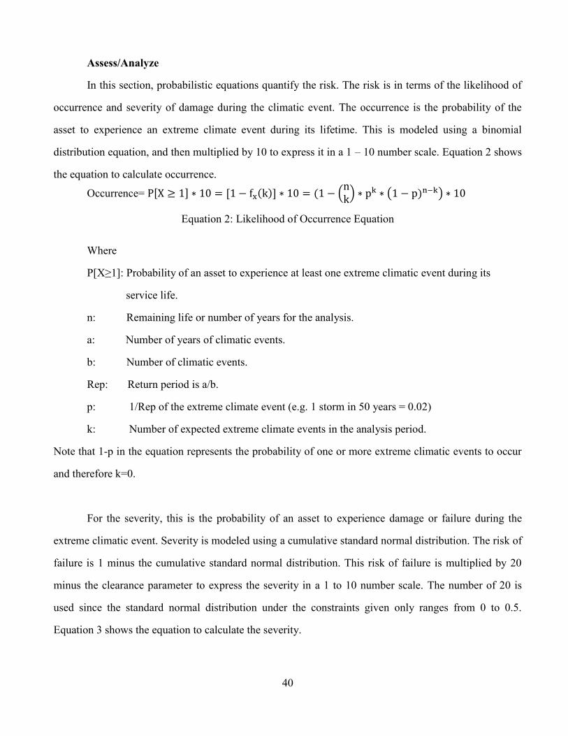
40
Assess/Analyze
In this section, probabilistic equations quantify the risk. The risk is in terms of the likelihood of
occurrence and severity of damage during the climatic event. The occurrence is the probability of the
asset to experience an extreme climate event during its lifetime. This is modeled using a binomial
distribution equation, and then multiplied by 10 to express it in a 1 – 10 number scale. Equation 2 shows
the equation to calculate occurrence.
Occurrence= P[X ≥ 1] ∗ 10 = [1 − fx(k)] ∗ 10 = (1 − (nk
) ∗ pk ∗ (1 − p)n−k) ∗ 10
Equation 2: Likelihood of Occurrence Equation
Where
P[X≥1]: Probability of an asset to experience at least one extreme climatic event during its
service life.
n: Remaining life or number of years for the analysis.
a: Number of years of climatic events.
b: Number of climatic events.
Rep: Return period is a/b.
p: 1/Rep of the extreme climate event (e.g. 1 storm in 50 years = 0.02)
k: Number of expected extreme climate events in the analysis period.
Note that 1-p in the equation represents the probability of one or more extreme climatic events to occur
and therefore k=0.
For the severity, this is the probability of an asset to experience damage or failure during the
extreme climatic event. Severity is modeled using a cumulative standard normal distribution. The risk of
failure is 1 minus the cumulative standard normal distribution. This risk of failure is multiplied by 20
minus the clearance parameter to express the severity in a 1 to 10 number scale. The number of 20 is
used since the standard normal distribution under the constraints given only ranges from 0 to 0.5.
Equation 3 shows the equation to calculate the severity.

41
Severity= P[Z < 0] ∗ (20 − Cp) = (1 − Φ(Z)) ∗ (20 − Cp)=(1 − Φ (ln (R
L))) ∗ (20 − Cp)
Equation 3: Severity Equation
Where
P[Z< 0]: Probability an asset to experience failure or damage at the time of occurrence of the
extreme climate event.
Φ(Z): Cumulative standard normal distribution.
R: Resistance parameter (e.g. height of bridge, volumetric capacity of culvert, etc.)
L: Acting parameter or climate stressor that can cause failure (e.g. height of storm surge,
flow due to heavy precipitation, etc.)
Cp: Clearance Parameter (R - L)
The risk of failure is expressed in terms of the occurrence and severity. The level of risk is then
assigned using the risk quantification chart shown in Figure 24.
Figure 24: Level of Risk Quantification Chart
To identify assets at high risk, the Failure Modes and Effects Analysis (FMEA) proposes a Risk
Priority Number (RPN). The RPN was proposed by the University of Colorado Denver (UC Denver). It
calculated the RPN by multiplying the likelihood of occurrence, severity, and detection based on surveys
and expert opinion to determine the occurrence, severity, and detection. The detection factor is scaled

42
from 1 to 10 (detectable to undetectable) and aims to measure if the risk could be detected (UC Denver
2004).
In the methodology proposed in this thesis, the detection is replaced by significance.
Significance is used to express the level of importance of an asset to the agency in a 1 to 10 scale.
Equation 4 shows the calculation for the RPN.
RPN = Occurrence * Severity * Significance
Equation 4: Risk Priority Number Equation
Assets that are vital to an agency or places more people’s lives at risk if it fails will have a higher
significance value than non-vital assets. An example of this can be seen in assets in an evacuation route
would have a higher significance than those that are not.
Mitigate and Plan
In this section of the risk analysis matrix, recommended actions are described. Actions can vary
from inspecting the asset more frequently to repair or reconstruction. Other mitigation and adaptation
strategies were previously discussed in Chapter 3.
Allocate
The implementation of the actions are assigned/allocated to a person or group or persons
responsible for the asset’s preservation. This can vary between assets depending on who manages them.
An example of this, are highways are managed by DOTs while arterial roadways are managed by
Metropolitan Planning Organizations (MPO).
Monitor and Control
In the last section, the asset is reevaluated using the RPN. This is to determine if there is a
reduction of the risk due to the actions recommended in the plan. Occurrence and severity are
recalculated for the asset to determine the level of risk. The risk reduction can be measured by
comparing the RPNs.
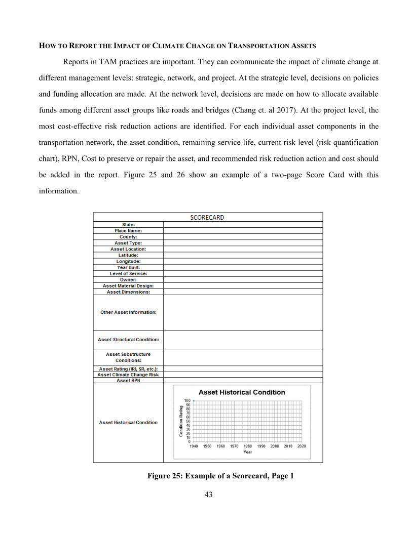
43
HOW TO REPORT THE IMPACT OF CLIMATE CHANGE ON TRANSPORTATION ASSETS
Reports in TAM practices are important. They can communicate the impact of climate change at
different management levels: strategic, network, and project. At the strategic level, decisions on policies
and funding allocation are made. At the network level, decisions are made on how to allocate available
funds among different asset groups like roads and bridges (Chang et. al 2017). At the project level, the
most cost-effective risk reduction actions are identified. For each individual asset components in the
transportation network, the asset condition, remaining service life, current risk level (risk quantification
chart), RPN, Cost to preserve or repair the asset, and recommended risk reduction action and cost should
be added in the report. Figure 25 and 26 show an example of a two-page Score Card with this
information.
Figure 25: Example of a Scorecard, Page 1

44
Figure 26: Example of a Scorecard, Page 2

45
Performance measures to show the impact of climate change at the network and strategic levels
are necessary to assist agencies and help with the awareness of the assets at risk. Specific performance
measures specific to climate change are recommended. Some examples of the performance measures are
as follows:
a. Percent of transportation assets (e.g. bridges, rails, etc.) that are affected by climatic events
(e.g. flooding, storm surge, etc.).
b. Percent of asset components in an asset group at high, medium, or low risk based on the RPN
and the Risk Quantification Chart.
c. Percent of essential evacuation routes affected by a climatic event.
d. Number of people affected by the climatic event.
It is important to present these performance measures in a concise and easy to understand form. Figure
27 and Figure 28 show an example of how to represent this information graphically. Figure 27 shows the
percent of asset components in each asset group at different levels at risk and Figure 28 displays an
example of the population at risk due to a climatic event. It is important to note that the data in these
figures are not representative of any specific agency and is only provided as an example. For both
figures, the left would show the current condition and the right would show the projected results.
Figure 27: Assets at Risk of Failure Due to Climate Events

46
Figure 28: Population at Risk of Failure Due to Climate Events
Graphs like these can be used in the reports to easily show the number of assess at each risk
level. They can also show the consequences in the future, if no actions are taken and the benefits of the
risk mitigation practices implemented by the agency. GIS maps are also recommended to be included in
the reports. The maps can help visually identify the location of the assets at risk due to climate change.
As climate change continues to affect weather patterns, resilience must be included into TAM
practices. To measure resilience, a Life Cycle Analysis (LCA) must be conducted as seen in Figure 29.
The figure also shows how an extreme climatic event will appears as a vertical line in the life cycle
indicating a loss of service life.
Figure 29: Asset Resilience in LCA (Minaie 2016)
The next sections illustrate the impact on the asset condition due to an extreme climatic event.
The events result in the loss of service life. Condition is a measurement of asset health. Remaining
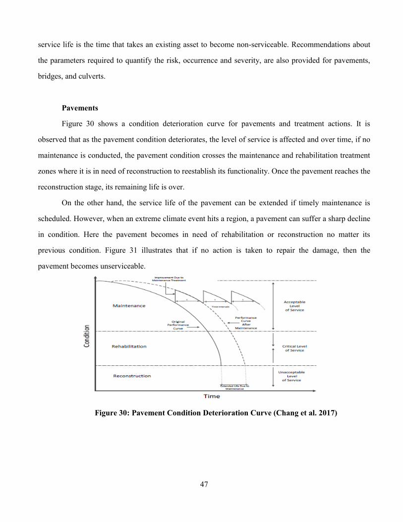
47
service life is the time that takes an existing asset to become non-serviceable. Recommendations about
the parameters required to quantify the risk, occurrence and severity, are also provided for pavements,
bridges, and culverts.
Pavements
Figure 30 shows a condition deterioration curve for pavements and treatment actions. It is
observed that as the pavement condition deteriorates, the level of service is affected and over time, if no
maintenance is conducted, the pavement condition crosses the maintenance and rehabilitation treatment
zones where it is in need of reconstruction to reestablish its functionality. Once the pavement reaches the
reconstruction stage, its remaining life is over.
On the other hand, the service life of the pavement can be extended if timely maintenance is
scheduled. However, when an extreme climate event hits a region, a pavement can suffer a sharp decline
in condition. Here the pavement becomes in need of rehabilitation or reconstruction no matter its
previous condition. Figure 31 illustrates that if no action is taken to repair the damage, then the
pavement becomes unserviceable.
Figure 30: Pavement Condition Deterioration Curve (Chang et al. 2017)

48
Figure 31: Pavement Condition and the Effect of Sever Climatic Events
An extreme climate event affects the entire pavement network. Figure 32 shows the percentage
of pavements in very good/good, and poor/very poor conditions over time in normal working conditions,
where the percentage of pavements in state of good repair decreases, the number of pavements in poor
condition starts to increase. Figure 33 illustrates that a situation where if an extreme climate event
occurred in 2016, then there will be a spike on the graph.
Figure 32: Projection of Pavement Condition Categories over Time in Normal Working
Conditions (Chang et al. 2017)

49
Figure 33: Projection of Pavement Condition Categories over Time Affected by an
Extreme Climate Event
To quantify the level of risk of pavements in terms of occurrence and severity, data should be
collected for the specific climatic event that threatens the pavement network. For example, for flooding,
the number of floods in a time period are needed to calculate the occurrence. For the severity, the R
parameter can be the pavement profile elevation, and the L parameter the height of the water in the
flood.
Bridges and Culverts
Figure 34 shows an example of the service life trend for timber and gravel bridges under normal
working conditions. The NBI is used by the Federal Highway Administration to evaluate the bridge
condition and varies from 9 to 0 (excellent to fail condition) as seen in Table 8.
Figure 34: Bridge Deterioration Curve for Timber and Gravel Bridges in Normal Working
Conditions (Chang et al. 2017)

50
Table 8: National Bridge Inventory General Condition Rating (FHWA 2011)
NBI
Rating Description
Commonly
Employed
Feasible Actions
9 Excellent condition. Preventive
maintenance 8 Very good condition, no problems noted.
7 Good condition, some minor problems.
6 Satisfactory condition, structural elements can show some
minor deterioration. Preventive
maintenance
and/or repairs 5
Fair condition, all primary structural elements are sound
but may have some minor section loss, cracking, spalling
or scour.
4 Poor condition, advanced section loss, deterioration,
spalling or scour.
Rehabilitation or
replacement
3 Serious condition, loss of section, deterioration, spalling or
scour have seriously affected primary structural elements.
2
Critical condition, advanced deterioration of primary
structural elements. Unless closely monitored the bridge
may have to be closed until corrective action is taken.
1
Imminent failure condition, major deterioration or section
loss present in critical structural components or obvious
vertical or horizontal movement affecting structure
stability. Bridge is closed to traffic but corrective action
may put back in light service.
0 Failed condition, out of service – beyond corrective action Replacement
The bridge condition deterioration curve shown in Figure 35 is an example for a particular type
of bridge. The NCHRP 859 research report recommends that “it is often helpful to develop different
deterioration curves depending on traffic, climate, or other factors” (Chang et al. 2017). Figure 35 shows
the service life of the bridge could be interrupted by an extreme climatic event, suddenly decreasing the
NBI condition rating.
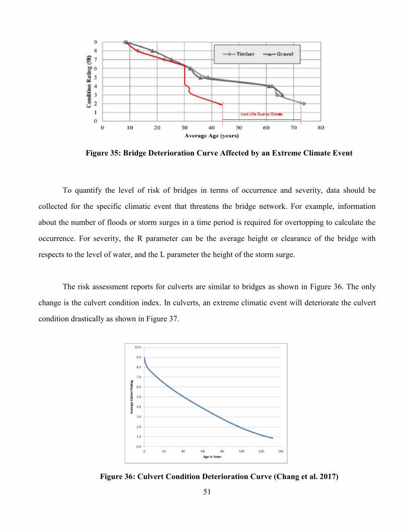
51
Figure 35: Bridge Deterioration Curve Affected by an Extreme Climate Event
To quantify the level of risk of bridges in terms of occurrence and severity, data should be
collected for the specific climatic event that threatens the bridge network. For example, information
about the number of floods or storm surges in a time period is required for overtopping to calculate the
occurrence. For severity, the R parameter can be the average height or clearance of the bridge with
respects to the level of water, and the L parameter the height of the storm surge.
The risk assessment reports for culverts are similar to bridges as shown in Figure 36. The only
change is the culvert condition index. In culverts, an extreme climatic event will deteriorate the culvert
condition drastically as shown in Figure 37.
Figure 36: Culvert Condition Deterioration Curve (Chang et al. 2017)

52
Figure 37: Culvert Deterioration Curve Affected by an Extreme Climatic Event
To quantify the level of risk of culverts in terms of occurrence and severity, data should be
collected for the specific climatic event that threatens them like floods. Since a culvert is constraint by
the capacity of water it can push through, then to calculate the severity the R parameter can be the
current capacity of the culvert. The L parameter can be the flow caused by heavy precipitation. R and L
parameters can also be simplified adopting for the calculations the height of the culvert and the flood
surge height respectively.
Economic Impact
Another type of reports to show the effects of extreme climatic events in a region are those that
include economic performance measures. These economic measures are: the Current Employment
Statistics (Establishment Survey), Current Population Survey (CPS) (Household Survey), Local Area
Unemployment Statistics (LAUS), Job Openings and Labor Turnover Survey (JOLTS), Producer Price
Indexes (PPI), Consumer Price indexes (CPI), Import and Export Price indexes (MXP), and the
Employment Cost Index (ECI). Table 9 provides a brief description of these performance measures.
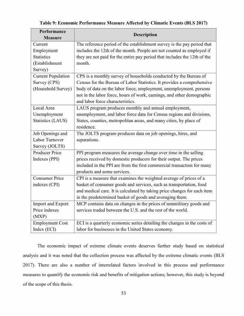
53
Table 9: Economic Performance Measure Affected by Climatic Events (BLS 2017)
Performance
Measure Description
Current
Employment
Statistics
(Establishment
Survey)
The reference period of the establishment survey is the pay period that
includes the 12th of the month. People are not counted as employed if
they are not paid for the entire pay period that includes the 12th of the
month.
Current Population
Survey (CPS)
(Household Survey)
CPS is a monthly survey of households conducted by the Bureau of
Census for the Bureau of Labor Statistics. It provides a comprehensive
body of data on the labor force, employment, unemployment, persons
not in the labor force, hours of work, earnings, and other demographic
and labor force characteristics.
Local Area
Unemployment
Statistics (LAUS)
LAUS program produces monthly and annual employment,
unemployment, and labor force data for Census regions and divisions,
States, counties, metropolitan areas, and many cities, by place of
residence.
Job Openings and
Labor Turnover
Survey (JOLTS)
The JOLTS program produces data on job openings, hires, and
separations.
Producer Price
Indexes (PPI)
PPI program measures the average change over time in the selling
prices received by domestic producers for their output. The prices
included in the PPI are from the first commercial transaction for many
products and some services.
Consumer Price
indexes (CPI)
CPI is a measure that examines the weighted average of prices of a
basket of consumer goods and services, such as transportation, food
and medical care. It is calculated by taking price changes for each item
in the predetermined basket of goods and averaging them.
Import and Export
Price indexes
(MXP)
MCP contains data on changes in the prices of nonmilitary goods and
services traded between the U.S. and the rest of the world.
Employment Cost
Index (ECI)
ECI is a quarterly economic series detailing the changes in the costs of
labor for businesses in the United States economy.
The economic impact of extreme climate events deserves further study based on statistical
analysis and it was noted that the collection process was affected by the extreme climatic events (BLS
2017). There are also a number of interrelated factors involved in this process and performance
measures to quantify the economic risk and benefits of mitigation actions; however, this study is beyond
of the scope of this thesis.

54
Chapter 5: Analysis of a Case Study for Bridges and Pavements
CASE STUDY INTRODUCTION
This chapter introduces a case study for a bridge and a roadway section to demonstrate the
applicability of the framework and methodology proposed to quantify the risk of asset damage due to
extreme climatic events.
In August 29, 2005, Hurricane Katrina made landfall and caused over “1800 lives lost and
caused major flooding and damage that spanned more than 2000 miles along the Gulf Coast of the
United States” (O’Connor and McAnany 2008). This hurricane was selected since it significantly
affected the New Orleans, Louisiana region. Levees, commercial and public buildings, roads and
bridges, utility distribution systems for electric power and water, wastewater collection facilities, and
vital communication networks suffered significant damaged due to the hurricane. Winds from the
hurricane were estimated at “125 mph and storm surges as high as 25 feet” (O’Connor and McAnany
2008). Prior to landfall, Hurricane Katrina gained strength to a “Category 5 while in the Gulf of Mexico,
but quickly dissipated to a Category 3 before landfall” (O’Connor and McAnany 2008). When
Hurricane Katrina made landfall, “the wind speeds were substantially reduced before striking land, but
the storm surge apparently maintained the heights associated with a Category 5“ (O’Connor and
McAnany 2008).
In this Chapter, the case studies presented demonstrate how the risk is quantified for individual
projects. The process can be extended to all the asset components in the asset group network. In order to
fully apply the framework, an agency must look at all assets at the network management level. It is
important to note that the examples presented in this Chapter have already occurred, although the
method must be applied to analyze future climate threats to the infrastructure.
I-10 TWIN SPAN BRIDGE CASE STUDY
The bridge selected for this case study was the old I-10 Twin Span Bridge located over Lake
Pontchartrain. In 2005, this bridge was heavily damaged during Hurricane Katrina. This study compares

55
the risk assessment for the old I-10 Twin Span Bridge and the newly-constructed I-10 Twin Span Bridge
that replaced the old bridge after Hurricane Katrina.
Step 1: Bridge Goals and Policies
Following the framework proposed, the first step is to identify the goals and policies to maintain
the bridge. Since the proposed bridge is in Louisiana, the goals and policies of the Louisiana Department
of Transportation are reviewed in this step and summarized in Table 10. The complete list of goals,
objectives and performance measures are in Appendix A.
Table 10: Goals and Objectives Relating to I-10 Twin Span Bridge
Goal Area Objectives
Infrastructure
Preservation and
Maintenance
Keep Louisiana’s state highway pavement, bridges, and highway
related assets in good condition.
Assist modal partners in achieving state-of-good-repair for aviation,
port, rail, transit, and navigable waterway infrastructure.
Safety
Reduce the number and rate of highway-related crashes, fatalities,
and serious injuries.
Assist modal partners in achieving safe and secure aviation, port,
rail, transit, and waterway performance.
Economic
Competitiveness
Improve the efficiency of freight transportation and the capacity of
freight related infrastructure throughout Louisiana.
Improve access to intermodal facilities and the efficiency of
intermodal transfers.
Provide predictable, reliable travel times throughout Louisiana.
Ensure small urban areas (5,000+ population) are well connected
with one another and with large urban employment centers.
Environmental
Stewardship
Minimize the environmental impacts of building, maintaining, and
operating Louisiana’s transportation system.
Comply with all federal and state environmental regulations
Since the goals and objectives presented are general, performance measures that directly
correlate climate change with asset conditions at the network level should be added. An example of this
can be the number of bridges at high, medium, or low risk of damage by an extreme climatic event.
Objective must also be specific and quantifiable to monitor the progress. For example, to preserve 90
percent of the bridges in the state of good repair or at low risk is a great objective that is specific and
quantifiable.
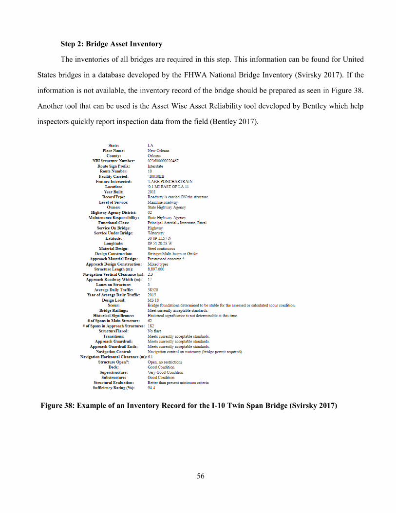
56
Step 2: Bridge Asset Inventory
The inventories of all bridges are required in this step. This information can be found for United
States bridges in a database developed by the FHWA National Bridge Inventory (Svirsky 2017). If the
information is not available, the inventory record of the bridge should be prepared as seen in Figure 38.
Another tool that can be used is the Asset Wise Asset Reliability tool developed by Bentley which help
inspectors quickly report inspection data from the field (Bentley 2017).
Figure 38: Example of an Inventory Record for the I-10 Twin Span Bridge (Svirsky 2017)

57
Step 3: Bridge Condition Assessment
In this step, the current condition of the bridge is determined and stored in the database from step
2. For our case study, Figure 38 also shows the current condition of the New Twin Span Bridge in terms
of the sufficiency rating. The Sufficiency Rating “is a weighted average comprised calculated by
combining scores for structural adequacy and safety (55 percent weight), serviceability and functional
obsolescence (30 percent weight), essentiality for public use (15 percent weight), and special reductions
(6 percent weight). Sufficiency Rating ranges between 0 for entirely deficient bridge and 100 for entirely
sufficient bridge” (Chang et al. 2017).
To show the effects of Hurricane Katrina on the old Twin Span Bridge, assumptions on the prior
condition of the bridge were made. The bridge was originally built in 1965 and when Hurricane Katrina
made landfall, the Twin Span Bridge was almost 50 years old. Using the deterioration model for bridges
described in Chapter 4, and assuming that only routine maintenance was conducted, the bridge would
have been in fair condition (NBI condition rating = 5). Figure 39 displays the bridge condition before
Hurricane Katrina.
Figure 39: Condition Assessment for I-10 Twin Span Bridge before Hurricane Katrina

58
Step 4: Bridge Risk Assessment
In this step, climate scenarios are formulated to assess the risk of bridge failure. In our case
study, the climate scenario for analysis is the storm surge, which is the most critical parameter that
affected the bridges of New Orleans. The following climatic impact scenarios are analyzed:
a. Scenario 1: High risk impact scenario that corresponds to a Category 5 Hurricane with a
storm surge of 25 ft.
b. Scenario 2: Medium risk impact scenario that corresponds to a Category 3 Hurricane with a
storm surge of 15 ft.
c. Scenario 3: Low risk impact scenario that corresponds to a Category 1Hurricane with a storm
surge of 5 ft.
The old I-10 Twin Span Bridge had a 9 ft elevation from the surface of the water (Abu-Farsakh
et al. 2014). To quantify the risk of damage, the occurrence and severity need to be calculated using the
equations from Chapter 4. For occurrence, the NOAA Historical Hurricane Tracks toolkit is used to
determine the frequency of the hurricanes (NOAA 2017). Appendix B contains the data for the
calculations. For severity, HR is the clearance of the bridge deck and the water level in feet. HL is the
height of potential storm surge height in feet. Cp is the clearance of the bridge and storm surge height.
The RPN is then calculated by multiplying the occurrence, severity, and significance. Note that since the
case study is conducted for an individual bridge, the significance is assumed to be 1 in the RPN
calculations. Tables 14 and 15 show the complete analysis for occurrence and severity respectively.

59
Table 11: I-10 Twin Span Bridge Occurrence, 9ft Clearance
Table 12: I-10 Twin Span Bridge Severity, 9ft Clearance
The acronyms Table 11 for the Hurricane category are TD for tropical depression, TS for tropical
storms, H1 for Hurricane Category 1, H2 for Hurricane Category 2, H3 for Hurricane Category 3, H4 for
Hurricane Category 4, and H5 for Hurricane Category 5. The three risk impact climatic scenarios
analyzed are highlighted. The number of years of historical data is the amount of historic data available

60
from the first event recorded until now. The asset life was arrived under the assumption that the asset
had a remaining service life of 50 years. This can also be interpreted as analyzing the asset in the next 50
years.
Table 12 also shows the three risk impact climate scenarios that were analyzed highlighted. As
expected, a higher storm surge would result in a higher Severity. The Cp values can show that when the
water has reached the height of the bridge and when the bridge has overtopped. When the Cp is zero, the
water level has reached the height of the bridge. When the Cp becomes negative, that shows how many
feet the bridge has been overtopped by.
Using both values from the occurrence and severity tables, the risk assessment matrix for each
climatic scenario and potential causes of failure for the old I-10 Twin Span Bridge can be populated in
Table 13.
Table 13: Risk Assessment Matrix for the I-10 Twin Span Bridge
Step 5: Bridge Needs (Gap) Analyses
In this step, the agency looks at the different actions and economic costs needed to action to
maintain, rebuild, or replace the bridge. In this case, the I-10 Twin Span Bridge repair cost was an
estimated $30 million, but just repairing the bridge would result in the same risk as before (Padgett et al.
2009). The cost to build the new twin span bridge was estimated at $800 million (LTRC n.d., Abu-
Farsakh 2014).
For the analysis, the Occurrence of new I-10 Twin Span Bridge was recalculated using a design
life of 100-years. For the severity the changes made were increasing the HR to the new clearance of the
bridge and water level in feet. HL remained the height of potential storm surge in feet and the Cp is the

61
new clearance for the storm surge. Tables 14 and 15 show the analysis for the occurrence and severity
respectively in the new risk assessment. The RPN values are also recalculated for the recommended
actions to deduce the level of risk.
Table 14: I-10 Twin Span Bridge Occurrence, 30ft Clearance
Table 15: I-10 Twin Span Bridge Severity, 30ft Clearance

62
In Table 14, an increase of the occurrence due to the longer analysis period and Hurricane
Katrina can be seen and in Table 15 a reduction in severity due to the height of the bridge is seen. With
both values the revisited risk and RPN can be tabulated as shown in Table 16. This table also shows that
each scenario could need different levels of investment.
Table 16: Risk Analysis Matrix for Reevaluation of the I-10 Twin Span Bridge
Step 6: Bridge Scenario Analyses
In this step, the three climate risk impact scenarios are evaluated with two budget scenarios. The
RPNs calculated previously in step 4 and step 5 are compared. As stated previously, since the case study
is conducted for an individual bridge, the significance is assumed to be 1 in the RPN calculations. For
the I-10 Twin Span Bridge, the percent of risk reduction of each scenario is shown in Tables 17 and 18
for $800 million and $30 million budgets respectively.
Table 17: Percent of Risk Reduction for the I-10 Twin Span Bridge Rebuilt, 30 ft Clearance and
$800 Million Budget

63
Table 18: Percent of Risk Reduction for the I-10 Twin Span Bridge Repair, 9 ft Clearance and $30
Million Budget
The percent of risk reduction for rebuilding of the bridge with a 30 ft clearance is 0% for a
Category 5 Hurricane with a 25 ft storm surge, 88% for a Category 3 Hurricane with a 15 ft storm surge,
and 75% for a Category 1 Hurricane with a 5 ft storm surge. Although there was no risk reduction for a
Category 5, the severity was reduced. Table 18 shows that there is no risk reduction if the bridge is just
repaired.
Step 7: Bridge Asset Management Report
In this step, a report is prepared to communicate decision-makers with the levels of risk for
climate scenarios. The risk reduction calculated in step 6 is expressed through the difference between the
RPNs. Figures 40 and 41 show the scorecard for the I-10 Twin Span Bridge before the landfall of
Hurricane Katrina as an example of how to report an asset at risk.

64
Figure 40: I-10 Twin Span Bridge Scorecard, Page 1

65
Figure 41: I-10 Twin Span Bridge Scorecard, Page 2

66
In combination with the scorecards, GIS tools can be used for analysis and reporting purposes.
GIS maps can facilitate in the location of the assets at risk in a region. For the example in the case study,
Figure 42 shows the level of risk of a storm surge condition of the old bridge. Figure 43 shows the level
of risk after the new bridge was built for a Category 3 Hurricane. These reports can be useful when
prioritizing budget allocations and identifying assets at high risk based on the RPN.
Figure 42: RPN GIS Map, Old I-10 Twin Span Bridge

67
Figure 43: RPN GIS Map, New I-10 Twin Span Bridge
Step 8: Bridge Asset Management Program to Mitigate the Impacts of Climate Change
Figure 44 shows the condition rating over time of the Twin Span Bridge. This includes
construction of the new bridge (Abu-Farsakh 2014). The mitigation strategy conducted for this bridge
was to raise the elevation of the bridge to reduce the risk of failure. It is important to note that this case
study was conducted for an individual project but the agency should apply the risk analysis to all the
assets to fully implement the framework in TAM practices. Also, the TAM framework with risk
mitigation practices requires to reevaluate future climate change threats. The recommendation is to
maintain historical records of the bridge condition and maintenance treatments over time to calibrate the
bridge condition deterioration models. Climate change information with performance predictions should
also be recorded to periodically review the climate change models.

68
Figure 44: Condition Rating Over Time for the I-10 Twin Span Bridge
ROAD IN FRANKLIN AVENUE
In 2005, Hurricane Katrina heavily damaged many roads in Louisiana. The road selected for the
case study is located on Franklin Avenue between Robert E. Lee Blvd. and Fillmore Av. in New
Orleans, Louisiana.
Step 1: Roads Goals and Policies
This step is similar to in the bridge section and begins by identifying the goals and policies to
maintain the roads. Since the proposed roads are in Louisiana, a check must be conducted on the goals
and policies of the governing agency who controls the asset. In this case, the goals, objectives, and
performance measures of the Regional Planning Commission (RCP) are summarized in Table 19. The
RCP serves as a reference for the New Orleans Metropolitan Planning Organization.

69
Table 19: Summary of Goals and Objectives in New Orleans Metropolitan Planning Organization
(RPC 2015)
Goal Area Objectives Performance Measures
Safety
Reduce the number of serious
injuries and fatalities resulting
from auto crashes by 50% by
2030.
Reduce the number of pedestrian
and bicyclist accidents by 50%
by 2030
Assist transit agencies in
reducing transit vehicle
accidents per 1,000,000
vehicles.
Annual number of serious injuries or fatalities
Annual number of serious injuries or fatalities
per vehicle mile travelled
Annual number of serious pedestrian injuries
or fatalities
Annual number of serious bicycle injuries and
fatalities
Transit vehicle accidents per 1,000,000
vehicle revenue miles.
State of Good
Repair
Complete a full conditions
inventory of the Congestion
Management System every four
years
Select and implement roadway
overlay and rehabilitation
projects
Assist transit agencies in
reducing the average number of
miles between in‐service failures
on regional fixed route transit
service
Percentage of Congestion Management
System roadway condition data collected
annually
Miles of roadway overlays or rehabilitation
completed annually
Average miles between in‐service failures on
regional fixed route service
Economic
Competitiveness
Invest in projects that improve
freight movements on the
National Highway System
Invest in projects that are in and
will benefit economically
depressed areas
Invest in projects that are in and
will benefit areas that have
predominantly minority
populations
Invest in projects that are in and
will benefit employment centers
Miles of roadway improvements on National
Highway System completed annually
Number of street overlay or transportation
enhancement projects within census tracts
with an average median household income at
or below the poverty level completed annually
Number of street overlay or transportation
enhancement projects within census tracts that
are predominantly minority completed
annually
Number of street overlay or transportation
enhancement projects in identified
employment centers

70
Table 19: Summary of Goals and Objectives in New Orleans Metropolitan Planning Organization
(RPC 2015) (cont’d)
Goal Area Objectives Performance Measures
Environmental
Sustainability
Encourage the increased use of
clean fuels in public and private
fleets.
Implement projects that
encourage transportation choices
beyond single‐occupancy
vehicle
Consider the potential future
impacts of change in the
planning and implementation of
roadway construction projects.
Reductions in traditional fuel consumption in
gasoline gallons equivalent by participants in
the Southeast Louisiana Clean Fuel
Partnership
Unlinked passenger trips on all regional
transit
Number of projects that increase roadway
grade or otherwise improve resiliency against
sea level rise or natural disasters
Similar to bridges, these are general goals and objectives. Therefore, performance measures that
directly correlate with climate change with asset conditions are recommended at the network level. An
example of this can be, the number of roads at high, medium, or low risk of damage by an extreme
climatic event. Very specific objectives are also recommended. This can be to preserve 90 percent of
roads in a state of good repair, or reduce 30% of roads from high to low risk.
Step 2: Roads Asset Inventory
Similar to the bridge inventory, the inventories of all the roads are required. Figure 45 shows an
example of the information recommended in an inventory road record. Additional information in the
road inventory record is required to quantify the risk of flooding. Figure 46 displays an elevation profile
for the section of road below from an online tool developed by the U.S. Geological Survey called The
National Map online tool (USGS 2017).
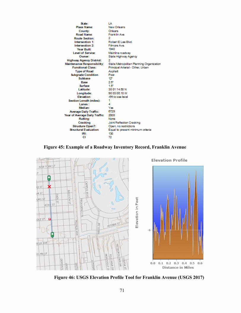
71
Figure 45: Example of a Roadway Inventory Record, Franklin Avenue
Figure 46: USGS Elevation Profile Tool for Franklin Avenue (USGS 2017)

72
Step 3: Road Condition Assessment
The Pavement Condition Index (PCI) is used to assess the road condition and is calculated from
individual pavement distresses recorded in the field based on severity and quantity. It ranges from 0 to
100 (very poor condition to very good condition). Table 20 shows the pavement condition categories are
defined with the PCI.
Table 20: CI and Pavement Condition
Category CI Condition
I 91-100 Very Good
II 71-90 Good
III 51 – 70 Fair
IV 25-50 Poor
V Under 25 Very Poor
Due to the lack of data on the roadway, assumptions were made and it was assumed that the PCI
was below a PCI of 50 before Hurricane Katrina as shown in Figure 47.
Figure 47: Condition Assessment for Franklin Ave. Road Section
Step 4: Road Risk Assessment
In this step, climate scenarios are formulated to assess the risk of road failure. Since “most of the
levee failures were caused by overtopping, as the storm surge rose over the top of a levee and scoured

73
out the base of the landward embankment or floodwall”, the climate scenarios for analysis are the same
as for the storm surge described in the I-10 Twin Span Bridge case study (Kayen et al. 2006). The
following climatic impact scenarios are analyzed:
a. Scenario 1: High risk impact scenario that corresponds to a Category 5 Hurricane with a
storm surge of 25 ft.
b. Scenario 2: Medium risk impact scenario that corresponds to a Category 3 Hurricane with a
storm surge of 15 ft.
c. Scenario 3: Low risk impact scenario that corresponds to a Category 1Hurricane with a storm
surge of 5 ft.
Prior to Hurricane Katrina, the levees were 15 ft high. To quantify the risk of damage, the
occurrence and severity again need to be calculated using the equations from Chapter 4. For occurrence,
the NOAA Historical Hurricane Tracks toolkit is used to determine the frequency of the hurricanes with
a levee in a 100-year return period (NOAA 2017). Appendix B contains the data for the calculations. For
severity, HR is the current height of the levee and the water level in feet. HL is the height of potential
storm surge height in feet. The Cp is the clearance of the levee and the storm surge height in feet. The
RPN is then calculated by multiplying the occurrence, severity, and significance. Note that since the
case study is conducted for an individual case, the significance is assumed to be 1 in the RPN
calculations. Tables 21 and 22 show the complete analysis for occurrence and severity respectively.
Table 21: Franklin Avenue Flooding Occurrence, 15ft Levees

74
Table 22: Franklin Avenue Flooding Severity, 15ft Levees
In both of the tables, the scenarios are highlighted. The occurrence shows that there is a high
probability that an asset will experience a hurricane Category 1 and 3 in the next 100 years. The
occurrence table also shows that the asset has a lower probability of experiencing a hurricane Category 5
in the next 100 years. The severity table shows that the asset will experience damage in a hurricane
Category 3 and 5 while little to no damage on a hurricane Category 1.
Using both values from the occurrence and severity tables, the risk assessment matrix for each
climatic scenario and potential causes of failure are seen in Table 23.

75
Table 23: Risk Assessment Matrix for Franklin Avenue
Step 5: Road Needs (Gap) Analyses
In this step, an agency again identifies different actions and budget needs to repair or rebuild the
road. In this case, the road flooding being analyzed is an indirect result of the levees and the repair cost
of the levees was estimated at $14.5 billion (Llanos 2015). New Orleans also build a 26-feet Storm
Surge Barrier that cost of $1.1 billion (Llanos 2015).
Using the NOAA Historical Hurricane Tracks toolkit to determine the number of hurricanes,
Table 24 shows the occurrence for the 17 ft levees and the storm surge barrier (NOAA 2017). Table 25
shows the recalculation of severity for the increased levee elevation. Table 26 shows recalculation of
severity for the storm surge barrier. For the increased levee elevation, HR is the new clearance of the
levee and the water level in feet, HL remains the height of storm surge in feet, and Cp is recalculated
with the new clearance with the storm surge. For the storm surge barrier, HR is the height of the storm
barrier. The RPN values are recalculated for the actions recommended to reduce the level of risk.

76
Table 24: Franklin Avenue Flooding Occurrence, 17ft Levees and 26ft Surge Barrier
Table 25: Franklin Avenue Flooding Severity, 17ft Levees

77
Table 26: Franklin Avenue Flooding Severity, 26ft Surge Barrier
In the tables, the scenarios are highlighted. Table 24 shows the same occurrence with the added
Hurricane and similar analysis period and Table 25 shows a slight reduction to severity in a hurricane
Category 3. Table 26 shows a reduction in severity in both hurricane Category 3 and 5. Using both the
occurrence and the two severity tables, Table 27 shows the tabulated risk and cost of each action.
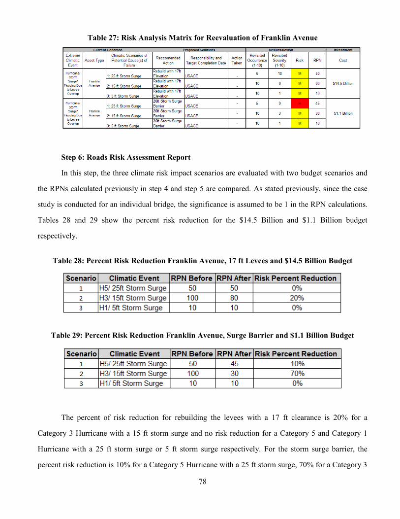
78
Table 27: Risk Analysis Matrix for Reevaluation of Franklin Avenue
Step 6: Roads Risk Assessment Report
In this step, the three climate risk impact scenarios are evaluated with two budget scenarios and
the RPNs calculated previously in step 4 and step 5 are compared. As stated previously, since the case
study is conducted for an individual bridge, the significance is assumed to be 1 in the RPN calculations.
Tables 28 and 29 show the percent risk reduction for the $14.5 Billion and $1.1 Billion budget
respectively.
Table 28: Percent Risk Reduction Franklin Avenue, 17 ft Levees and $14.5 Billion Budget
Table 29: Percent Risk Reduction Franklin Avenue, Surge Barrier and $1.1 Billion Budget
The percent of risk reduction for rebuilding the levees with a 17 ft clearance is 20% for a
Category 3 Hurricane with a 15 ft storm surge and no risk reduction for a Category 5 and Category 1
Hurricane with a 25 ft storm surge or 5 ft storm surge respectively. For the storm surge barrier, the
percent risk reduction is 10% for a Category 5 Hurricane with a 25 ft storm surge, 70% for a Category 3

79
Hurricane with a 15 ft storm surge, and there is no risk reduction for a Category 1 Hurricane with a 5 ft
storm surge.
Step 7: Road Asset Management Report
In this step, a report is prepared to communicate decision-makers with the levels of risk for
climate scenarios. The risk reduction calculated in step 6 is expressed through the difference between the
RPNs. By upgrading the levee to 17 ft high and building the storm surge barrier, the level of risk is
reduced. Figures 48 and 49 show the scorecard for road before the landfall of Hurricane Katrina as an
example of how to report an asset at risk.
Figure 48: I-10 Twin Span Bridge Scorecard, Page 1
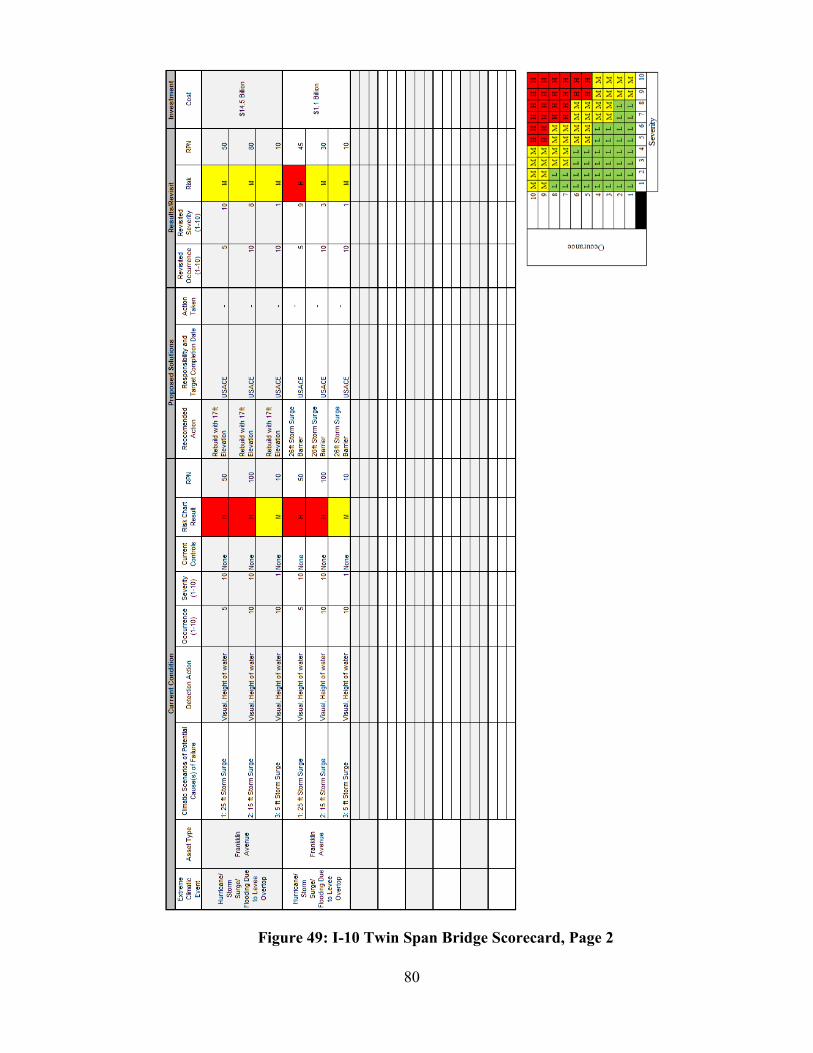
80
Figure 49: I-10 Twin Span Bridge Scorecard, Page 2
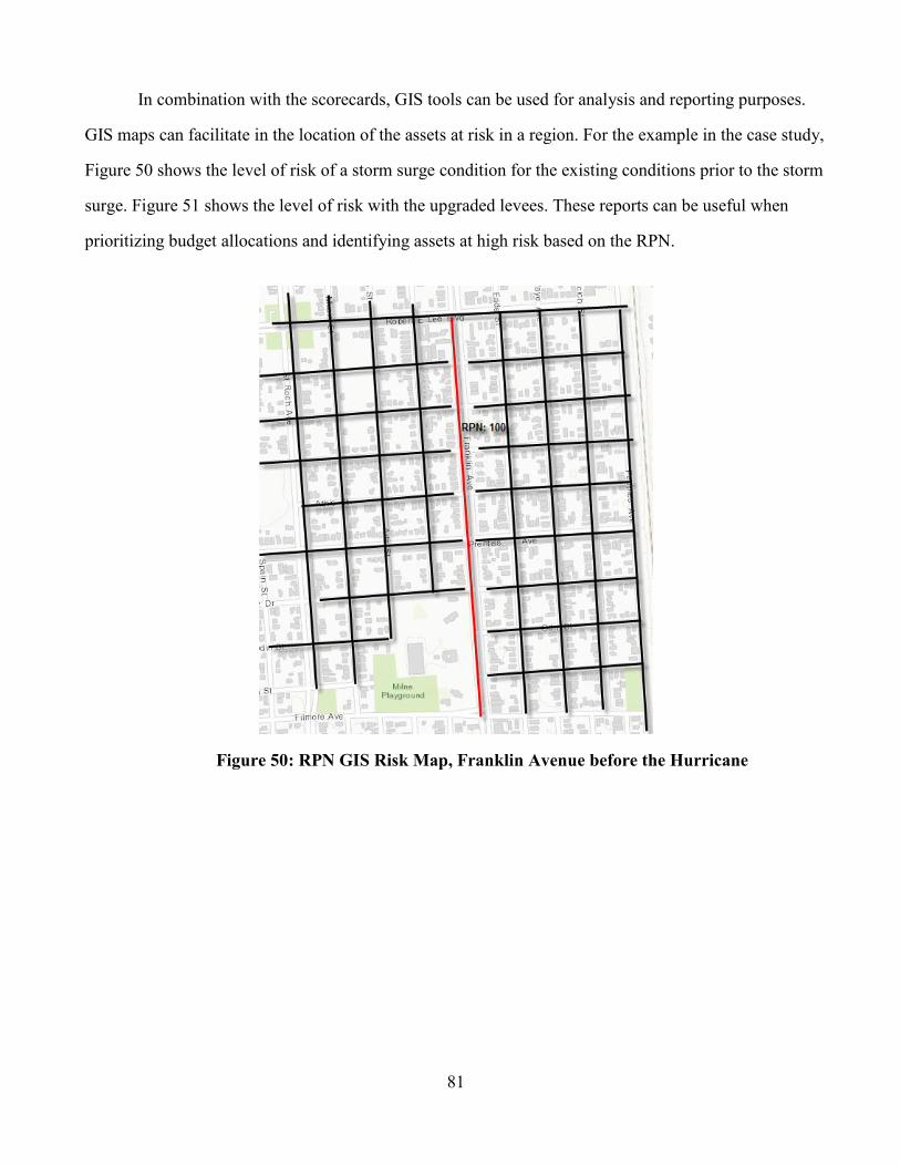
81
In combination with the scorecards, GIS tools can be used for analysis and reporting purposes.
GIS maps can facilitate in the location of the assets at risk in a region. For the example in the case study,
Figure 50 shows the level of risk of a storm surge condition for the existing conditions prior to the storm
surge. Figure 51 shows the level of risk with the upgraded levees. These reports can be useful when
prioritizing budget allocations and identifying assets at high risk based on the RPN.
Figure 50: RPN GIS Risk Map, Franklin Avenue before the Hurricane

82
Figure 51: RPN GIS Risk Map, Franklin Avenue after Recommended Actions
Step 8: Road Asset Management Program to Mitigate the Impacts of Climate Change
The roadway presented in this case study is 6 ft below sea level. The risk mitigation strategy
was to raise the elevation of the levees and build a storm surge barrier. Figure 52 shows the projected
PCIs after repairing the road. Similar to the bridge example, the road case study was for an individual
project. It is important to note that the agency should apply the risk analysis to all the roads to fully
implement the framework in TAM practices. The same recommendations as for the bridge case study
apply to the road network.

83
Figure 52: PCI over time for the Franklin Avenue Road after Recommended Actions

84
Chapter 6: Results and Discussion of the Climate Risk Assessment Model
This chapter provides a discussion of the climate risk assessment model through a sensitivity
analysis of the parameters used to quantify the risk of damage. The sensitivity analyses are conducted to
identify the most relevant parameters for occurrence and severity. TopRank is the software used to
perform “what if” analysis to determine the sensitivity of the outcomes. @Risk is the software used to
perform the Monte Carlo simulations in order to analyze the likelihood of alternative scenarios to occur
(Palisade 2017). Monte Carlo simulations of severity, occurrence, and RPN are performed in this
chapter.
OCCURRENCE
The risk assessment model determines the probability of occurrence of a climate event which has
three inputs for the occurrence to analyze. The inputs are the Number of Years of Climatic Events (a),
the Number of Events (b), and the Remaining Asset Life (n). The number of years of climatic events is
the years from the first climatic event recorded to the last year of the analysis. The asset remaining life is
the number of years that the asset is expected to remain in service. Figure 53 shows the Excel formulas
used to calculate the occurrence.
Figure 53: Excel Formulas for Occurrence
For hurricanes, the first input in the model is the number of events. From historical records, the
number of events is extracted using a Countif function. When modeling for events in the future events, a
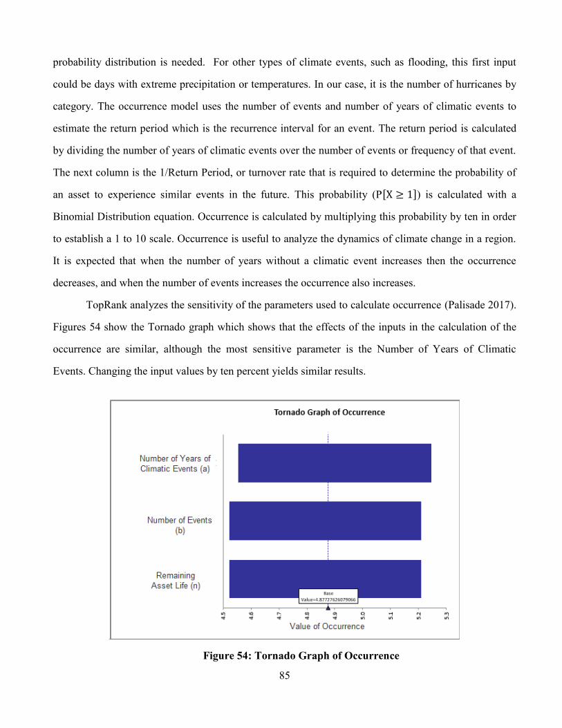
85
probability distribution is needed. For other types of climate events, such as flooding, this first input
could be days with extreme precipitation or temperatures. In our case, it is the number of hurricanes by
category. The occurrence model uses the number of events and number of years of climatic events to
estimate the return period which is the recurrence interval for an event. The return period is calculated
by dividing the number of years of climatic events over the number of events or frequency of that event.
The next column is the 1/Return Period, or turnover rate that is required to determine the probability of
an asset to experience similar events in the future. This probability (P[X ≥ 1]) is calculated with a
Binomial Distribution equation. Occurrence is calculated by multiplying this probability by ten in order
to establish a 1 to 10 scale. Occurrence is useful to analyze the dynamics of climate change in a region.
It is expected that when the number of years without a climatic event increases then the occurrence
decreases, and when the number of events increases the occurrence also increases.
TopRank analyzes the sensitivity of the parameters used to calculate occurrence (Palisade 2017).
Figures 54 show the Tornado graph which shows that the effects of the inputs in the calculation of the
occurrence are similar, although the most sensitive parameter is the Number of Years of Climatic
Events. Changing the input values by ten percent yields similar results.
Figure 54: Tornado Graph of Occurrence

86
Figure 55 shows the spider graph for occurrence, which shows the correlation between the
number of years of climatic events, the number of events, and the asset life. It is observed that as the
number of years of climatic data increases the occurrence decreases and if the remaining asset life of
climatic event increases or the number of events increases, then the occurrence increases.
Figure 55: Spider Graph of Occurrence
With @Risk to conduct Monte Carlo simulations, the Remaining Asset Life is modeled with a
Weibull distribution as shown in Figures 56. Weibull distributions are often used to model the length of
life and endurance data (Yoe 2012). The Number of Years of climatic events is modeled with a uniform
distribution as shown in Figure 57, which has a minimum at 162 years that refers to the years in the
existing records, and a maximum at 262 years. The maximum value of 262 years is obtained by adding
the remaining asset life to the number of years of climatic events in order to evaluate the asset
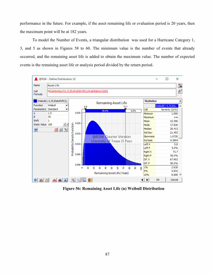
87
performance in the future. For example, if the asset remaining life or evaluation period is 20 years, then
the maximum point will be at 182 years.
To model the Number of Events, a triangular distribution was used for a Hurricane Category 1,
3, and 5 as shown in Figures 58 to 60. The minimum value is the number of events that already
occurred, and the remaining asset life is added to obtain the maximum value. The number of expected
events is the remaining asset life or analysis period divided by the return period.
Figure 56: Remaining Asset Life (n) Weibull Distribution
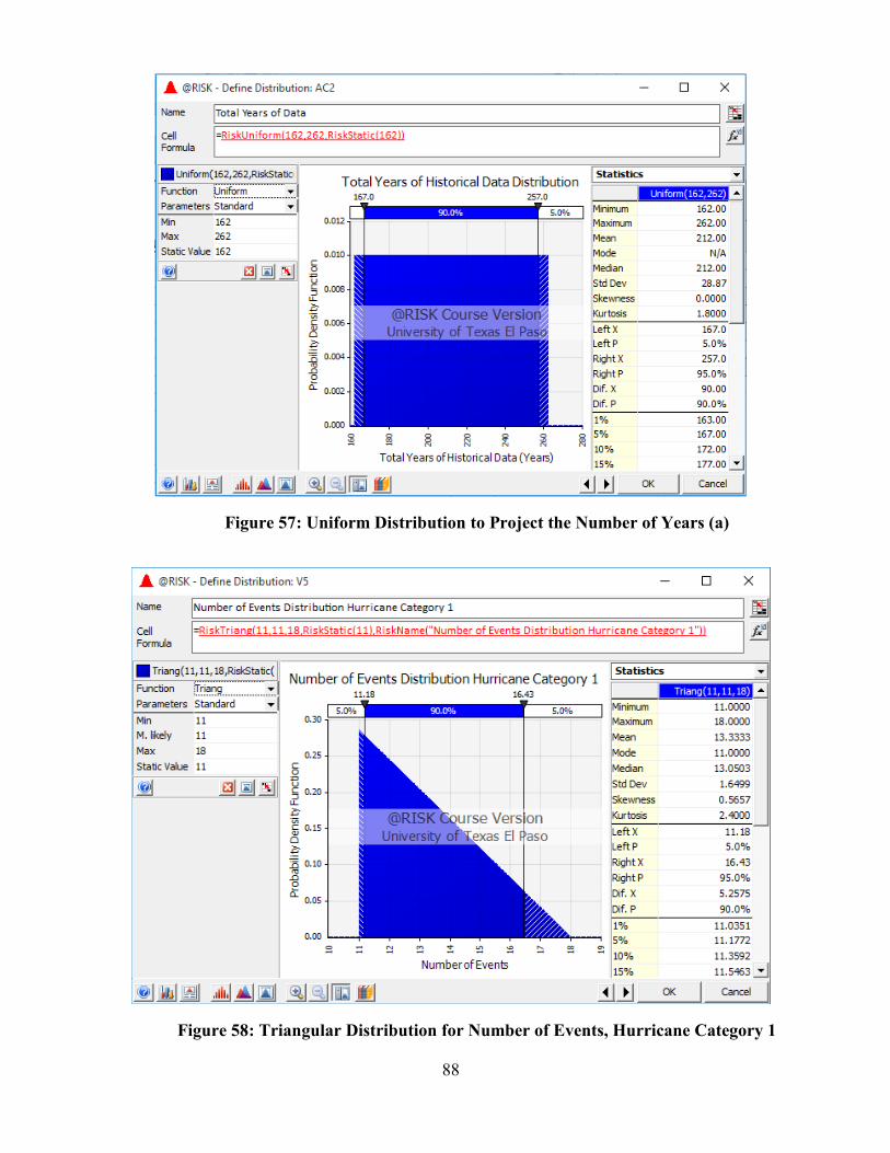
88
Figure 57: Uniform Distribution to Project the Number of Years (a)
Figure 58: Triangular Distribution for Number of Events, Hurricane Category 1
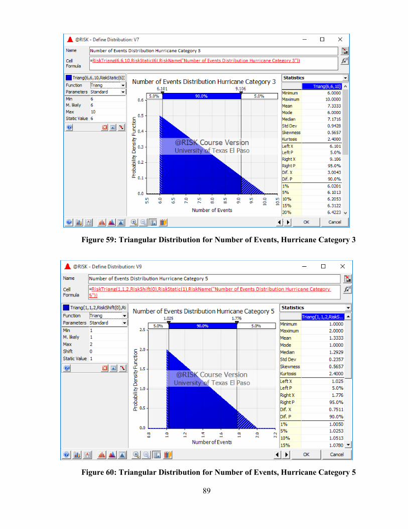
89
Figure 59: Triangular Distribution for Number of Events, Hurricane Category 3
Figure 60: Triangular Distribution for Number of Events, Hurricane Category 5
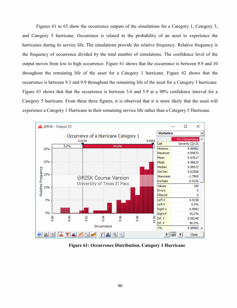
90
Figures 61 to 63 show the occurrence outputs of the simulations for a Category 1, Category 3,
and Category 5 hurricane. Occurrence is related to the probability of an asset to experience the
hurricanes during its service life. The simulations provide the relative frequency. Relative frequency is
the frequency of occurrence divided by the total number of simulations. The confidence level of the
output moves from low to high occurrence. Figure 61 shows that the occurrence is between 9.9 and 10
throughout the remaining life of the asset for a Category 1 hurricane. Figure 62 shows that the
occurrence is between 9.3 and 9.9 throughout the remaining life of the asset for a Category 3 hurricane.
Figure 63 shows that that the occurrence is between 3.6 and 5.9 at a 90% confidence interval for a
Category 5 hurricane. From these three figures, it is observed that it is more likely that the asset will
experience a Category 1 Hurricane in their remaining service life rather than a Category 5 Hurricane.
Figure 61: Occurrence Distribution, Category 1 Hurricane

91
Figure 62: Occurrence Distribution, Category 3 Hurricane
Figure 63: Occurrence Distribution, Category 5 Hurricane

92
SEVERITY
The following figure, Figure 64, shows the Excel formulas used to calculate the severity.
Figure 64: Excel Formulas for Severity
For hurricanes, there are two input parameters for severity. The parameters are the resistance and
the acting. HR, is the resistance parameter. HL is the acting parameter that can damage the asset. The
model calculates the severity for a given HR. The parameters are used for storm surge in this example,
but the resistance and acting may be represented by other parameters in other type of climate events. For
example, in track buckling the HR is the spacing in the track and HL is the track expansion due to high
temperatures.
In Figure 64, HR, the resisting parameter, is the height of a bridge. HL, the resisting parameter, is
the Storm Surge. In the next step, a Cumulative Normal Standard Probability of the natural log of the
resisting parameter over the acting value is calculated, and the probability of failure is calculated by
subtracting 1 from this probability. The clearance number is obtained by subtracting HR from HL. The
severity is obtained by multiplying the risk times 20 minus the clearance. Since the severity calculation
may be lower than 1 or higher than 10, an “If statement” formula is needed to be within the 1 to 10
range.
TopRank sensitivity analysis results are shown with Tornado graph, Figure 65 and Spider graph
Figure 65. The Tornado graph shows that HR is the most sensitive parameter for severity.

93
Figure 65: Tornado Graph of Severity
The spider graph in Figure 66 shows the correlation between HR and HL whereas the HR
increases the severity decreases. Also as HL decreases then the severity decreases.
Figure 66: Spider Graph of Severity
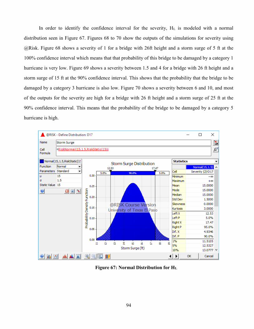
94
In order to identify the confidence interval for the severity, HL is modeled with a normal
distribution seen in Figure 67. Figures 68 to 70 show the outputs of the simulations for severity using
@Risk. Figure 68 shows a severity of 1 for a bridge with 26ft height and a storm surge of 5 ft at the
100% confidence interval which means that that probability of this bridge to be damaged by a category 1
hurricane is very low. Figure 69 shows a severity between 1.5 and 4 for a bridge with 26 ft height and a
storm surge of 15 ft at the 90% confidence interval. This shows that the probability that the bridge to be
damaged by a category 3 hurricane is also low. Figure 70 shows a severity between 6 and 10, and most
of the outputs for the severity are high for a bridge with 26 ft height and a storm surge of 25 ft at the
90% confidence interval. This means that the probability of the bridge to be damaged by a category 5
hurricane is high.
Figure 67: Normal Distribution for HL

95
Figure 68: Severity Distribution, Category 1 Hurricane
Figure 69: Severity Distribution, Category 3 Hurricane

96
Figure 70: Severity Distribution, Category 5 Hurricane
RISK PRIORITY NUMBER (RPN)
To analyze the RPN confidence interval, occurrence and severity are combined using @Risk.
The RPN expresses the risk of failure due to a climatic event, and it is obtained by multiplying
occurrence and severity. Figures 71 to 73 show the RPN outputs of the simulations using the relative
frequency. Figure 71 shows RPN outputs between 9.9 to 10 for a bridge with 26 ft height and a storm
surge of 5 ft at the 90% confidence interval, which means that the bridge is at a low risk of damage by a
category 1 hurricane. Figure 72 shows RPN outputs between 12.1 and 40.8 for a bridge with 26 ft height
and a storm surge of 15 ft at the 90% confidence interval, which shows that the bridge is at a slightly
higher risk of damage by a category 3 hurricane. Figure 73 shows RPN outputs between 24.3 and 55.6
for a bridge with 26 ft height and a storm surge of 25 ft at the 90% confidence interval, which means
that there is a higher risk of damage by a category 5 hurricane.

97
Figure 71: RPN Relative Frequency Distribution, Category 1 Hurricane
Figure 72: RPN Relative Frequency Distribution, Category 3 Hurricane

98
Figure 73: RPN Relative Frequency Distribution, Category 5 Hurricane
Another way to represent the outcomes of the simulation is using the Cumulative Distribution
function. These are seen in Figures 74 to 76. The benefit of using this type of distribution, is that the
probability can be read directly. For example, in Figure 74, the probability that the RPN is 9.96 or lower,
is 20 percent for a hurricane 1.

99
Figure 74: RPN Cumulative Distribution, Category 1 Hurricane
Figure 75: RPN Cumulative Distribution, Category 3 Hurricane

100
Figure 76: RPN Cumulative Distribution, Category 5 Hurricane
101
Chapter 7: Conclusions and Recommendations
This chapter summarizes the research findings and recommendations as a result of the study
about the impact of extreme climatic events on the “State of Good Repair” of the transportation
infrastructure.
SUMMARY OF RESEARCH FINDINGS
a. The first objective of this research was to identify climate change threats, risks, and
performance measures on transportation infrastructure. The threats, risks, and performance
measures were summarized in Chapter 2. Climate change definition, causes, impact on
transportation infrastructure, laws on transportation (MAP-21 and FAST Act), and TAM
practices were reviewed. Climate change is the statistical shift of weather patterns. It is
caused by the Earth in response to human induced changes like CO2 emissions. The level of
service of transportation assets, including roads, bridges, culverts, and rails, is affected by
climate stressors that occur more frequently as a result of climate change. Examples of
climate stressors are increased temperature and extreme heat, precipitation-driven inland
flooding, sea level rise/extreme high tides, storm surge, winds, droughts, dust storms,
wildfires, winter storms, changes in freeze/thaw, and permafrost thaw. As a result of the
literature review, it was concluded that traditional TAM practices do not explicitly consider a
risk assessment for extreme climatic events. There is also a need to incorporate a
methodology to quantify the risk of damage of transportation assets.
b. The second objective of this research was to develop a framework to incorporate risk
assessment into TAM practices and criteria to prioritize funding allocation. A general
framework with eight main steps is presented. The steps are:
o Step 1: Goals and Policies
o Step 2: Asset Inventory
o Step 3: Condition Assessment
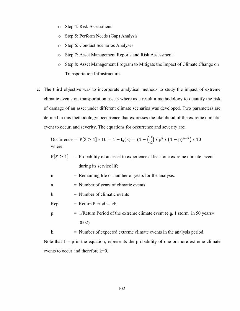
102
o Step 4: Risk Assessment
o Step 5: Perform Needs (Gap) Analysis
o Step 6: Conduct Scenarios Analyses
o Step 7: Asset Management Reports and Risk Assessment
o Step 8: Asset Management Program to Mitigate the Impact of Climate Change on
Transportation Infrastructure.
c. The third objective was to incorporate analytical methods to study the impact of extreme
climatic events on transportation assets where as a result a methodology to quantify the risk
of damage of an asset under different climate scenarios was developed. Two parameters are
defined in this methodology: occurrence that expresses the likelihood of the extreme climatic
event to occur, and severity. The equations for occurrence and severity are:
Occurrence = P[X ≥ 1] ∗ 10 = 1 − fx(k) = (1 − (nk
) ∗ pk ∗ (1 − p)n−k) ∗ 10
where:
P[𝑋 ≥ 1] = Probability of an asset to experience at least one extreme climate event
during its service life.
n = Remaining life or number of years for the analysis.
a = Number of years of climatic events
b = Number of climatic events
Rep = Return Period is a/b
p = 1/Return Period of the extreme climate event (e.g. 1 storm in 50 years=
0.02)
k = Number of expected extreme climate events in the analysis period.
Note that 1 – p in the equation, represents the probability of one or more extreme climate
events to occur and therefore k=0.

103
Severity =P[Z < 0] ∗ (20 − Cp) = (1 − Φ(Z)) ∗ (20 − Cp)
=(1 − Φ (ln (R
L))) ∗ (20 − Cp)
where:
P[𝑍 < 0] = Probability an asset to experience failure or damage at the time of
occurrence of the extreme climate event.
Φ(𝑍) = Cumulative standard normal distribution
R = Resistance parameter (e.g. height of bridge, volumetric capacity of culvert,
etc.)
L = Acting parameter or climate stressor that can cause failure (e.g. height of,
storm surge flow due to heavy precipitation, etc.)
Cp = Clearance Parameter (R - L)
Critical assets are identified by the Risk Priority Number (RPN) which is obtained by
multiplying occurrence, severity, and significance. Significance is a value from 1 to 10 and
an asset that is vital to the transportation infrastructure, or places more people’s lives at risk
if it fails will have a higher significance value. The higher the RPN of an asset, the higher the
priority for action. This is because the higher the RPN the higher the threat to preserve the
transportation infrastructure in a “State of Good Repair”.
In Chapter 6, a sensitivity analysis was conducted for occurrence and severity. For
occurrence, it was found that as the number of years without an extreme climatic event
increases, the occurrence decreases and if the remaining asset life increases, the occurrence
increases. For severity, it was observed that as the resisting parameter increases or, as the
acting parameter decreases, then severity decreases.
d. Two case studies were conducted to demonstrate the applicability of the framework and
methodology to quantify the risk of a bridge and a road. Both case studies relied upon
historical data from an extreme climatic event that already occurred. The occurrence and

104
severity were calculated to compare the level of risk before the event and after the solutions
(e.g. increasing the bridge height). The RPNs before and after the solutions, recommended
actions, were calculated to determine if the risk was reduced. Table 30 shows a summary of
the risk analysis for both case studies.
Table 30. Summary of the Analysis Results for the Case Studies
From these case studies, we learned that it is feasible to implement the framework and
methodology to quantify the risk of damage of existing assets due to climatic events as well
as the effects of mitigation and adaptation strategies.
e. The final objective of the study was to recommend practical adaptation strategies to mitigate
the impact of climate change threats. Some examples of adaptation strategies included
increasing the elevation of bridges, rail lines, and roadways, restrict development in
vulnerable areas, and relocation of roadway sections to less vulnerable areas. A list of
mitigation and adaptation strategies is presented in Chapter 4 where the benefits of adopting
the recommended mitigation strategies in an asset management program should be reflected
in the performance measures over time. Performance measures that directly correlate climate
change with asset conditions should also be reported (e.g. number of bridges at high,
medium, or low risk).
f. Summary reports with the results of the risk assessment analysis are needed to facilitate the
communication at the network and strategic management level. A scorecard with information

105
about the asset location, asset condition, remaining service life, current risk level, and RPN is
recommended. Examples of the scorecard were presented in the case studies in Chapter 5.
GIS is also considered a powerful communication tool to analyze and report risk assessment
results. For example, GIS dynamic maps are useful to visualize the location of the assets at
different levels of risk in the transportation infrastructure network.
RESEARCH CONTRIBUTIONS
The major contribution of this research is the development of a framework to consider climate
change impact in TAM practices. Another major contribution is the methodology to quantify the risk of
damage of an asset due to extreme climatic events. The risk of damage or failure is quantified by the
occurrence, severity, and risk priority number (RPN). The RPN can be used to prioritize assets for
funding allocation. The RPN can also be used to quantify the reduction of risk due to implementation of
proactive actions in the asset management program.
AREAS OF FUTURE RESEARCH AND DEVELOPMENT
a. In this case studies, the methodology to quantify risk was applied to individual assets. Further
research is needed to evaluate the risk of damage for the entire transportation infrastructure
network. The risk assessment of the entire network should consider all transportation assets
as interdepend and functioning together to provide the level of service desired by the agency.
b. The incorporation of sustainability performance measures to evaluate the vulnerability and
resilience of the entire network due to extreme climate events needs further study. Agency
goals for safety, mobility, and environment are affected by climate events, and there is a need
to investigate their impact in these areas.
c. It is recommended to implement a pilot web-based tool to monitor the level of risk in the
transportation infrastructure network. The web-based tool should be linked to a dynamic
inventory database with updated information about the asset conditions and treatment history.

106
The web-based tool could generate visual reports with the RPNs for all the asset components
that may be useful to prioritize investments.
d. Further research is needed to analyze the percent risk reduction to the cost. Currently, it is not
clear how much percent risk reduction is attributed to each dollar spent. The future research
should consider percent risk reduction per asset and try and correlate it to the amount of
dollars spent. A risk reduction network index may be also incorporated and related to the
investments made to improve the asset’s resiliency.
e. Finally, research is required to determine the economic impacts of climate change in a
region. In this sense, it is recommended to study the effect of extreme climate events on
economic performance measures including: Current Employment Statistics, Current
Population Survey (CPS), Local Area Unemployment Statistics (LAUS), Job Openings and
Labor Turnover Survey (JOLTS), Producer Price Indexes (PPI), Consumer Price indexes
(CPI), Import and Export Price indexes (MXP), and Employment Cost Index (ECI). A cost-
benefit study of the recommended strategies to mitigate the impact of extreme climate is also
a topic for future research.
107
References
Abu-Farsakh, M.Y., S. Yoon, X. Yu, and X. Tang. 2014. Structural Health Monitoring of I-10 Twin
Span Bridge. Department of Civil and Environmental Engineering. Louisiana State University.
Baton Rouge, LA 70803
Allen, C., M. Averso, C. Hargraves, and S. McNeil. 2015. Guide for the Preservation of Highway
Tunnel Systems. NCHRP Report 14-27. National Cooperative Highway Research Program,
Washington, D.C.
American Association of State Highway and Transportation Officials (AASHTO). 2012. Integrating
Extreme Weather Risk into Transportation Asset Management.
American Society of Civil Engineers (ASCE). 2009. Americas Infrastructure Reports Card 2009.
American Society of Civil Engineers (ASCE). 2013. Americas Infrastructure Reports Card 2013.
Arkansas Department of Transportation (ARDOT). 2014. Technical Memorandum #3 Goals and
Objectives. CDM Smith, Garver, and High Street Consulting Group.
Arkansas Department of Transportation (ARDOT). 2017. Technical Memorandum #4 A Performance
Measures. CDM Smith, Garver, and High Street Consulting Group.
Ashley, D. B., J. E. Diekmann, and K. R. Molenaar. 2006. Guide to Risk Assessment and Allocation for
Highway Construction Management. Federal Highway Administration. U.S. Department of
Transportation. Washington, DC.
Auber, A. 2011. Drought Effects Extend Far Beyond Water Restrictions. The New York Times.
February 5, 2017. http://www.nytimes.com/2011/08/05/us/05ttdrought.html.
Bentley. 2017. AssetWise Asset Reliability Inspection and Maintenance Management for Transportation
Infrastructure.
Bureau of Labor Statistics (BLS). 2017. Effects of Recent Hurricanes on BLS Data Collection and
Reporting. Washington, DC. https://www.bls.gov/bls/hurricanes-harvey-irma-maria.htm.
Accessed January 15, 2017.
Canon, S.H. and J. DeGraff. 2009. Cascading Consequences of Climate Change and Expanding
Population on the Threat of Wildfire and Post Fire Debris-Flow.
Chang, C.M., S. Nazarian, R.E. Smith, M. Vavrova, M.T. Yapp, L.M. Pierce, T. Punnackal, J.
Puccinelli, M. Lee, and W. Robert. 2017. Consequences of Delayed Maintenance of Highway
Assets. National Cooperative Research Program. NCHRP Report 14-20A.
Environmental Protection Agency (EPA). 2015. Climate Change Indicators in the United States: U.S.
and Global Temperature.
Environmental Protection Agency (EPA). 2016. Climate Impacts on Transportation. February 14, 2017.
https://www.epa.gov/climate-impacts/climate-impacts-transportation.
Federal Highway Administration (FHWA). 1999. Asset Management Primer. U.S. Department of
Transportation.
Federal Highway Administration (FHWA). 2010. Regional Climate Change Effects: Useful Information
for Transportation Agencies. Federal Highway Administration, Washington, DC.
Federal Highway Administration (FHWA). 2011. Bridge Preservation Guide, Maintaining a State of
Good Repair Using Cost Effective Investment Strategies. Report No. FHWA-HIF-11-042.
Federal Highway Administration, Washington, DC.
Federal Highway Administration (FHWA). 2012. FHWA Vulnerability Assessment Framework. Federal
Highway Administration, Washington, DC.
Federal Highway Administration (FHWA). 2014. Gulf Coast Study Phase 1 & Phase II. Federal
Highway Administration, Washington, DC.

108
Federal Highway Administration (FHWA). 2016a. Fixing America’s Surface Transportation Act (FAST
Act): A Summary of Highway Provisions. Office of Policy and Governmental Affairs. March 14,
2017. https://www.fhwa.dot.gov/fastact/fastact_summary.pdf.
Federal Highway Administration (FHWA). 2016b. Asset Management Plans and Periodic Evaluations
of Facilities Repeatedly Requiring Repair and Reconstruction Due to Emergency Events. March
14, 2017. https://www.federalregister.gov/documents/2016/10/24/2016-25117/asset-
management-plans-and-periodic-evaluations-of-facilities-repeatedly-requiring-repair-and.
Federal Highway Administration (FHWA). 2017. Asset Management. U.S. Department of
Transportation. May 23, 2017. https://www.fhwa.dot.gov/asset/faq.cfm.
Froehlich, D. 2003. Sea-Level Rise Impacts on Scour at Coastal Bridges in the Southeastern United
States. Presented at the EGS - AGU - EUG Joint Assembly.
http://adsabs.harvard.edu/abs/2003EAEJA....13778F.
Grunwald, M. 2016. A new Obama emissions play. Politico, February 9, 2017.
http://www.politico.com/agenda/story/2016/04/a-new-obama-emissions-play-000095
House Transportation and Infrastructure Committee. 2015. Summary FAST ACT. March 14, 2017.
http://transportation.house.gov/uploadedfiles/house_senate_big_4.pdf.
Huang, Y. 1993. Pavement Analysis and Design. Prentice-Hall Inc. Englewood Cliffs, New Jersey
07632.
ICF International. 2014. Transportation Climate Change Sensitivity Matrix. U.S. Department of
Transportation. https://ceq.doe.gov/current_developments/GHG-accounting-tools.html.
Intergovernmental Panel on Climate Change (IPCC). 2014. Climate Change 2014: Synthesis Report.
Contribution of Working Groups I, II and III to the Fifth Assessment Report of the
Intergovernmental Panel on Climate Change. [Core Writing Team, R.K. Pachauri and L.A.
Meyer (eds.)]. IPCC, Geneva, Switzerland, 151 pp.
International Organization for Standardization (ISO) 55000. 2014. Asset Management Overview,
Principles and Terminology.
Kaufman, S., C. Qing, N. Levenson, and M. Hanson. 2012. Transportation During and After Hurricane
Sandy. Rudin Center for Transportation. NYU Wagner Graduate School of Public Service.
Kayen, R., B. Collins, and H. Gibbons. 2006. USGS Scientists Investigate New Orleans Levees Broken
by Hurricane Katrina. USGS. https://soundwaves.usgs.gov/2006/01/. Accessed August 15, 2017.
Liu. R., P. Xu, Z. Sun, X. Zou, and Q. Sun. 2015. Establishment of Track Quality Index Standard
Recommendations for Beijing Metro. Discrete Dynamics in Nature and Society Vol. 2015,
Article 473830, Pg. 9.
Llanos, M. 2015. Will New Orleans’ $14.5 Billion Walls Stand Up to the Next Big Storm? NBC News.
https://www.nbcnews.com/storyline/hurricane-katrina-anniversary/new-orleans-14-5-billion-
walls-n415816. Accessed September 1, 2017.
Louisiana Department of Transportation Plan (DOTD). 2015. Louisiana Statewide Transportation Plan.
CDM Smith.
Louisiana Transportation Research Center (LTRC). n.d. Featured Bridge Presentation/Tour I-10 Twin
Span Bridge.
Meyer, M., Amekudzi, A., and O’Har, J. 2010. Transportation Asset Management Systems and Climate
Change: An Adaptive Systems Management Approach. Transportation Research Record: Journal
of the Transportation Research Board, (2160), 12–20.
Minaie, E. 2016. Resilience and Transportation Asset Management: A Practical Approach. CDM Smith.
Ohio Transportation Engineering Conference.
National Oceanic and Atmospheric Administration (NOAA). 2007. Climate Change.
National Research Council (NRC). 2008. Transportation Research Board Special Report 290: Potential
Impacts of Climate Change on U.S. Transportation. Transportation Research Board.

109
National Oceanic and Atmospheric Administration(NOAA). 2017. U.S. Climate Resilience Toolkit.
https://toolkit.climate.gov/tools. Accessed July 15, 2017.
National Cooperative Highway Research Program (NCHRP). 2013. Response to Extreme Weather
Impacts on Transportation Systems. Transportation Research Board. Washington, D.C.
National Cooperative Highway Research Program (NCHRP). 2014. Strategic Issues Facing
Transportation, Volume 2: Climate Change, Extreme Weather Events, and the Highway System:
Practitioner s Guide and Research Report. Transportation Research Board. Washington, D.C.
New Mexico Department of Transportation (NMDOT). 2015. The New Mexico 2040 Plan NMDOT’s
Long Range , Multi-Modal Transportation Plan. Santa Fe, New Mexico.
O’Connor, J.S. and P.E. McAnany. 2008. Damage to Bridges from Wind, Storm Surge and Debris in the
Wake of Hurricane Katrina. MCEER Special Report Series: Engineering and Organizational
Issues, Before During and After Hurricane Katrina.
Oklahoma Department of Transportation (OKDOT). 2014. Visions, Goals, Objectives, and Performance
Measures. CDM Smith.
Orr, D., M. Kestler, T. Andersen, and G. Larson. 2017. Springtime Damage to Roads and Seasonal Load
Limits. Transportation Research Board. The National Academies of Sciences, Engineering, and
Medicine. Webinar.
Padgett, Jamie E., Spiller, April and Arnold, Candase. 2009. Statistical Analysis of Coastal Bridge
Vulnerability Based on Empirical Evidence from Hurricane Katrina. Structure and Infrastructure
Engineering
Palisade. 2017. @Risk & Decision Tools Suite Software. http://www.palisade.com/. Accessed January
15, 2018.
Regional Planning Commission (RPC). 2015. 2015-2044 Metropolitan Transportation Plan: New
Orleans Urbanized Area. New Orleans, LA.
Stenstrom, C., A. Parida, and D. Galar. 2012. Performance Indicators of Railway Infrastructure.
International Journal of Railway Technology Vol. 1, Issue 3, Pg. 1-18.
Svirsky, A. 2017. National Bridges. The National Bridges Inventory Database. Website:
http://www.nationalbridges.com/. Accessed January 18, 2017.
Texas Department of Transportation (TXDOT). 2014. Goals, Objectives, and Performance Measures.
Texas Freight Advisory Committee. Austin, Texas.
Texas Department of Transportation (TXDOT). 2015. Texas Transportation Plan 2040. Austin, Texas.
UK Highways Agency. 2011. Climate Change Risk Assessment August.
U.S. Department of Transportation (U.S. DOT). n.d. (a). Building Resilient Transportation. Federal
Highway Administration.
U.S. Department of Transportation (U.S. DOT). n.d. (b). Addressing Resilience in Project
Development: Living Shoreline along Coastal Roadways Exposed to Sea Level Rise. Federal
Highway Administration.
U.S. Department of Transportation (U.S. DOT). 2007. Asset Management Overview. Federal Highway
Administration. FHWA-IF-08-008. March 14, 2017.
U.S. Department of Transportation (U.S. DOT). 2013. Performance Management. MAP-21- Moving
Ahead for Progress in the 21st Century. https://www.fhwa.dot.gov/map21/factsheets/pm.cfm.
Accessed March 14, 2017.
U.S. Department of Transportation (U.S. DOT). 2015. Buckled Rails. U.S. Climate Resilience Toolkit.
March 14, 2017. https://toolkit.climate.gov/image/1001
U.S. Geological Survey (USGS). 2012. Post-Wildfire Landslide Hazards.
http://landslides.usgs.gov/research/wildfire/. Accessed February 28, 2017.
U.S. Geological Survey (USGS). 2017. The National Map. Toolkit.
https://viewer.nationalmap.gov/advanced-viewer/. Accessed August 28, 2017.
110
United Nations. 2013. Climate Change Impacts and Adaptation for International Transport Networks.
United States Government Publishing Office (USGPO). 2017. Federal Register. Vol. 82, No. 11,
Wednesday, January 18, 2017.
University of Colorado Denver (UC Denver). 2004. Failure Modes and Effects Analysis (FMEA).
Institute for Healthcare Improvement.
Verdin, K.L., J.A. Dupree, and J.G. Elliott. 2012. Probability and Volume of Potential Postwildfire
Debris Flows in the 2012 High Park Burn Area near Fort Collins, Colorado. U.S. Geological
Survey.
Washington State Department of Transportation (WSDOT). 2016. WSDOT Bridge Design Manual M
23-50.16.
West, J.S., C. J. Larosche, B. D. Koester, J.E. Breen, and M.E. Kreger. 1999. State of the Art Report
About Durability of Post-Tensioned Bridge Substructures. Center for Transportation Research.
The University of Texas at Austin.
Willway, T., S. Reeves, and L. Bldachin. 2008. Maintaining Pavements in a Changing Climate.
Department for Transport. UK Roads Board.
Yoe, C. 2012. Principles of Risk Analysis Decision Making Under Uncertainty. CRC Press. Sound
Parkway, NW 334

113
Appendix A
Goals, Objectives, and Performance Measures Used by the Southern Plain States
Table A-1. USDOT Main Goals and Performance Measures (USGPO 2017) ............................ 114
Figure A-1. TxDOT Goals Adaptation from MAP-21 (TxDOT 2015) ....................................... 115
Table A-2. TxDOT Goals and Objectives (TxDOT 2014, TxDOT 2015) .................................. 115
Table A-3. TxDOT Performance Measures (TxDOT 2014, TxDOT 2015) ................................ 118
Table A-4. NMDOT Goals and Objectives (NMDOT 2015) ...................................................... 119
Table A-5. NMDOT Performance Measures (NMDOT 2015) ................................................... 121
Table A-6. OkDOT Goals and Objectives (OkDOT 2014) ......................................................... 122
Table A-7. OkDOT Performance Measures (OkDOT 2014) ...................................................... 123
Table A-8. ArDOT Goals and Objectives (ArDOT 2014) .......................................................... 124
Table A-9. ArDOT Performance Measures (ArDOT 2017) ........................................................ 126
Table A-10. DOTD Goals and Objectives (DOTD 2015) ........................................................... 127
Table A-11. DOTD Performance Measures (DOTD 2015) ........................................................ 128
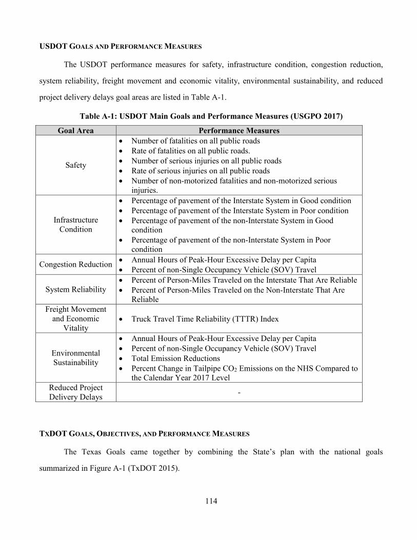
114
USDOT GOALS AND PERFORMANCE MEASURES
The USDOT performance measures for safety, infrastructure condition, congestion reduction,
system reliability, freight movement and economic vitality, environmental sustainability, and reduced
project delivery delays goal areas are listed in Table A-1.
Table A-1: USDOT Main Goals and Performance Measures (USGPO 2017)
Goal Area Performance Measures
Safety
Number of fatalities on all public roads
Rate of fatalities on all public roads.
Number of serious injuries on all public roads
Rate of serious injuries on all public roads
Number of non-motorized fatalities and non-motorized serious
injuries.
Infrastructure
Condition
Percentage of pavement of the Interstate System in Good condition
Percentage of pavement of the Interstate System in Poor condition
Percentage of pavement of the non-Interstate System in Good
condition
Percentage of pavement of the non-Interstate System in Poor
condition
Congestion Reduction Annual Hours of Peak-Hour Excessive Delay per Capita
Percent of non-Single Occupancy Vehicle (SOV) Travel
System Reliability
Percent of Person-Miles Traveled on the Interstate That Are Reliable
Percent of Person-Miles Traveled on the Non-Interstate That Are
Reliable
Freight Movement
and Economic
Vitality Truck Travel Time Reliability (TTTR) Index
Environmental
Sustainability
Annual Hours of Peak-Hour Excessive Delay per Capita
Percent of non-Single Occupancy Vehicle (SOV) Travel
Total Emission Reductions
Percent Change in Tailpipe CO2 Emissions on the NHS Compared to
the Calendar Year 2017 Level
Reduced Project
Delivery Delays -
TXDOT GOALS, OBJECTIVES, AND PERFORMANCE MEASURES
The Texas Goals came together by combining the State’s plan with the national goals
summarized in Figure A-1 (TxDOT 2015).

115
Figure A-1: TxDOT Goals Adaptation from MAP-21 (TxDOT 2015)
TxDOT’s objectives can be seen in Table A-2 corresponding to the goal areas of safety, asset
management, mobility and reliability, multimodal connectivity, stewardship, customer service, and
sustainable funding.
Table A-2: TxDOT Goals and Objectives (TxDOT 2015)
Goal Area Objectives
Safety
Improve multimodal transportation safety
Reduce fatalities and serious injuries
Improve safety of at-grade rail crossings
Eliminate conflicts between modes wherever possible
Increase bicycle and pedestrian safety through education, the design
and construction of new facilities, and improvements to existing
facilities
Educate the public on the dangers of high-risk driving behaviors
Coordinate with enforcement to improve
Improve incident response times

116
Table A-2: TxDOT Goals and Objectives (TxDOT 2015) (cont’d)
Goal Area Objectives
Asset Management
Maintain and preserve multimodal assets using cost-beneficial
treatments
Decrease the number of bridges that are structurally deficient,
functionally obsolete, or substandard-for-load
Achieve state of good repair for pavement assets, keeping pavements
smooth and pothole free
Achieve state of good repair for transit assets such that they are
comfortable and reliable
Identify and mitigate risks associated with asset failure
Identify existing and new funding sources and innovative financing
techniques for all modes of transportation
Build upon and regularly update the asset inventories for all
transportation modes
Mobility and
Reliability
Reduce congestion and improve system efficiency and performance
Plan, design, and construct strategic capacity projects
Implement alternative strategies that reduce peak demand
Improve operations within existing right-of-way
Increase travel options and accessibility for all, especially elderly,
disabled, and disadvantaged populations
Increase freight and passenger travel time reliability
Increase the capacity and efficiency of the transportation system
across travel modes
Multimodal
Connectivity
Provide transportation choices and improve system connectivity for
all passenger and freight modes
Provide and improve access to jobs, transportation choices, and
services for all Texans
Provide safe and convenient travel choices for all Texans with a
focus on the complete trip
Support the efficient and coordinated movement of goods and
services between freight modes to facilitate statewide, national, and
global commerce
Support multimodal and intermodal planning, project development,
and investments
Improve connectivity between urban, suburban, and rural areas and
between travel modes

117
Table A-2: TxDOT Goals and Objectives (TxDOT 2015) (cont’d)
Goal Area Objectives
Stewardship
Manage resources responsibly and be accountable and transparent in
decision-making
Identify sustainable funding sources and leverage resources wisely to
maximize the value of investments and minimize negative impacts
Develop and implement a project development process that
recognizes quality-of-life concerns for all system users and future
generations of Texans
Link transportation planning with land use
Reduce project delivery delays
Coordinate project planning and delivery with all planning partners
and stakeholders
Minimize impacts to natural, cultural, and historic resources and
promote sustainability in project design and delivery
Customer Service
Understand and incorporate customer desires in decision processes
and be open and forthright in all agency communications
Collect and integrate feedback using innovative engagement
techniques and technology
Promote and enable public participation in project planning and
development
Improve accessibility of information through innovative,
understandable, and relatable communication techniques
Educate the public and stakeholders on transportation costs, funding
availability, and investment tradeoffs
Sustainable Funding
Identify and sustain funding sources for all modes
Identify and document costs to meet the state’s future transportation
needs
Consider all funding sources to fill the needs-to-revenues gap
Educate the public and stakeholders on the costs associated with
constructing and preserving the system
Evaluate the feasibility of innovative financing solutions
Improve predictive capabilities for revenue forecasting and long-
term needs assessments
TxDOT’s performance measures are shown in Table A-3 corresponding to the goal areas of
safety, asset management, mobility and reliability, multimodal connectivity, stewardship, customer
service, and sustainable funding. Note that this Table has two references because one covers the
performance measures of freights.
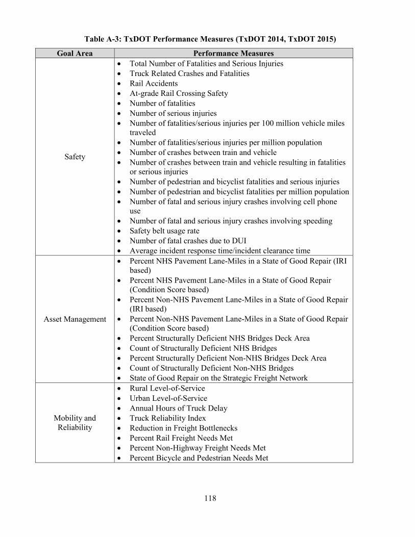
118
Table A-3: TxDOT Performance Measures (TxDOT 2014, TxDOT 2015)
Goal Area Performance Measures
Safety
Total Number of Fatalities and Serious Injuries
Truck Related Crashes and Fatalities
Rail Accidents
At-grade Rail Crossing Safety
Number of fatalities
Number of serious injuries
Number of fatalities/serious injuries per 100 million vehicle miles
traveled
Number of fatalities/serious injuries per million population
Number of crashes between train and vehicle
Number of crashes between train and vehicle resulting in fatalities
or serious injuries
Number of pedestrian and bicyclist fatalities and serious injuries
Number of pedestrian and bicyclist fatalities per million population
Number of fatal and serious injury crashes involving cell phone
use
Number of fatal and serious injury crashes involving speeding
Safety belt usage rate
Number of fatal crashes due to DUI
Average incident response time/incident clearance time
Asset Management
Percent NHS Pavement Lane-Miles in a State of Good Repair (IRI
based)
Percent NHS Pavement Lane-Miles in a State of Good Repair
(Condition Score based)
Percent Non-NHS Pavement Lane-Miles in a State of Good Repair
(IRI based)
Percent Non-NHS Pavement Lane-Miles in a State of Good Repair
(Condition Score based)
Percent Structurally Deficient NHS Bridges Deck Area
Count of Structurally Deficient NHS Bridges
Percent Structurally Deficient Non-NHS Bridges Deck Area
Count of Structurally Deficient Non-NHS Bridges
State of Good Repair on the Strategic Freight Network
Mobility and
Reliability
Rural Level-of-Service
Urban Level-of-Service
Annual Hours of Truck Delay
Truck Reliability Index
Reduction in Freight Bottlenecks
Percent Rail Freight Needs Met
Percent Non-Highway Freight Needs Met
Percent Bicycle and Pedestrian Needs Met
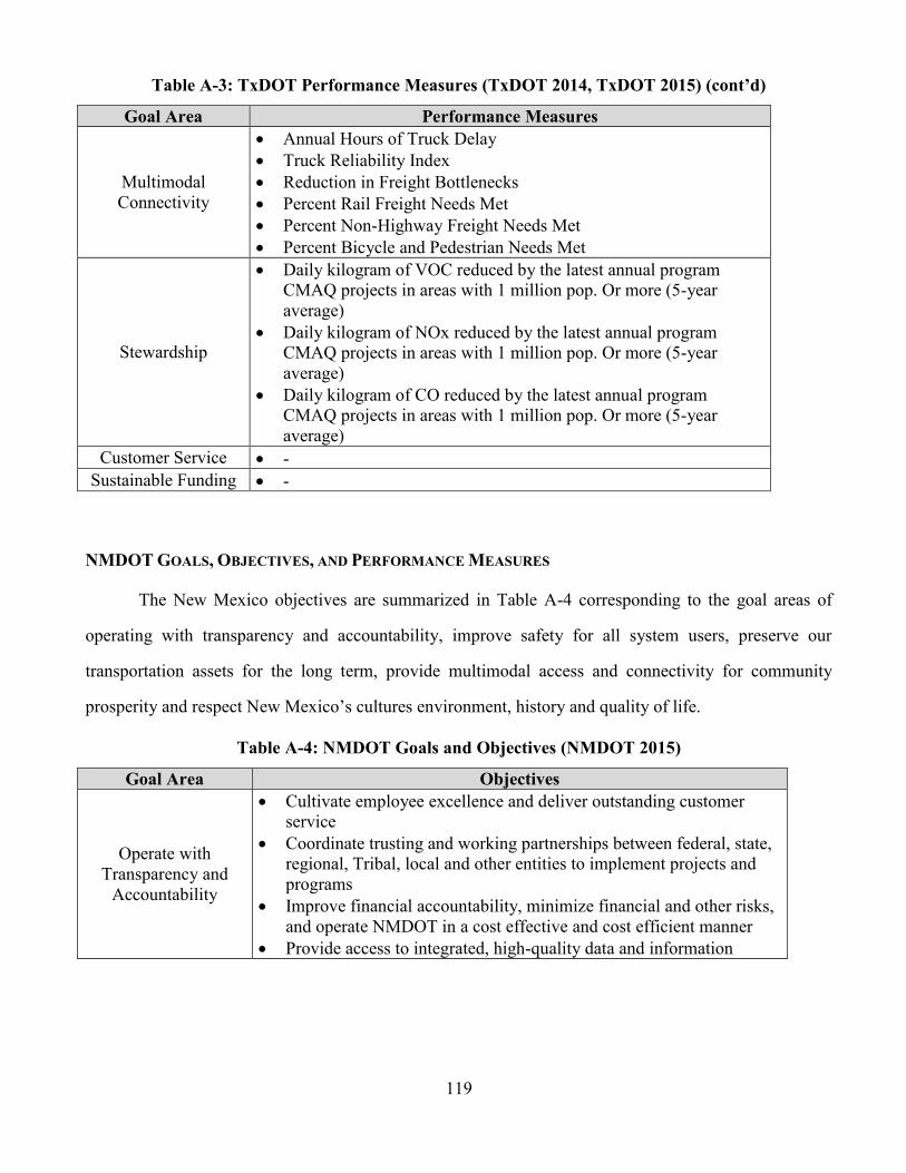
119
Table A-3: TxDOT Performance Measures (TxDOT 2014, TxDOT 2015) (cont’d)
Goal Area Performance Measures
Multimodal
Connectivity
Annual Hours of Truck Delay
Truck Reliability Index
Reduction in Freight Bottlenecks
Percent Rail Freight Needs Met
Percent Non-Highway Freight Needs Met
Percent Bicycle and Pedestrian Needs Met
Stewardship
Daily kilogram of VOC reduced by the latest annual program
CMAQ projects in areas with 1 million pop. Or more (5-year
average)
Daily kilogram of NOx reduced by the latest annual program
CMAQ projects in areas with 1 million pop. Or more (5-year
average)
Daily kilogram of CO reduced by the latest annual program
CMAQ projects in areas with 1 million pop. Or more (5-year
average)
Customer Service -
Sustainable Funding -
NMDOT GOALS, OBJECTIVES, AND PERFORMANCE MEASURES
The New Mexico objectives are summarized in Table A-4 corresponding to the goal areas of
operating with transparency and accountability, improve safety for all system users, preserve our
transportation assets for the long term, provide multimodal access and connectivity for community
prosperity and respect New Mexico’s cultures environment, history and quality of life.
Table A-4: NMDOT Goals and Objectives (NMDOT 2015)
Goal Area Objectives
Operate with
Transparency and
Accountability
Cultivate employee excellence and deliver outstanding customer
service
Coordinate trusting and working partnerships between federal, state,
regional, Tribal, local and other entities to implement projects and
programs
Improve financial accountability, minimize financial and other risks,
and operate NMDOT in a cost effective and cost efficient manner
Provide access to integrated, high-quality data and information

120
Table A-4: NMDOT Goals and Objectives (NMDOT 2015) (cont’d)
Goal Area Objectives
Improve Safety for
All System Users Reduce collision- related fatalities and serious injuries for all modes
through data-driven, innovative, and proactive processes
Preserve and
Maintain Our
Transportation Assets
for the Long Term
Develop and implement a “preservation-first” asset management
strategy to ensure that NMDOT can maintain all existing and future
elements of the state’s multimodal transportation system in a state of
good repair.
Ensure that NMDOT can affordably meet the minimum condition
standards for each roadway tier by right sizing the state-owned
network to provide the needed capacity to support statewide
connectivity standards.
Provide Multimodal
Access and
Connectivity for
Community
Prosperity
Invest efficiently and strategically in state transportation systems to
achieve statewide and community economic and quality of life goals.
Make efficient use of both transportation and nontransportation
resources to reduce costs and improve mobility of residents and
visitors.
Maintain a transportation system that allows mobility and access for
all New Mexicans, regardless of age or ability.
Respect New
Mexico’s Cultures,
Environment,
History, and Quality
of Life
Transportation projects and programs respect the context within
which they are built and implemented.
NMDOT seeks to improve environmental outcomes with both its
transportation investments and business operations.
NMDOT celebrates and advances New Mexico economic goals in
the areas of recreation and tourism.
Table A-5 shows the performance measures for New Mexico corresponding to the goal areas of
operating with transparency and accountability, improve safety for all system users, preserve our
transportation assets for the long term, provide multimodal access and connectivity for community
prosperity and respect New Mexico’s cultures environment, history and quality of life.

121
Table A-5: NMDOT Performance Measures (NMDOT 2015)
Goal Area Performance Measures
Operate with
Transparency and
Accountability
Percent of 2040 Plan actions completed within timeframe identified
in this plan
Public ratings of NMDOT in customer satisfaction survey
Percent of positions vacant in all programs
Stakeholder ratings of NMDOT in customer satisfaction survey
Percent of projects obligated versus programmed in the STIP
Percent of cost over bid amount
Number of annual external financial audit findings
Percent of prior year financial audit findings resolved
Percent of essential data sources updated on schedule [measurement
approach TBD]
Improve Safety for
All System Users
Total number of fatalities
Total fatalities per 100 million vehicle miles traveled (statewide,
rural, and urban)
Total number of serious injuries
Serious injuries per 100 million VMT (statewide, rural, and urban)
Pedestrian fatalities and serious injuries (statewide, rural, and
urban)*
Bicyclist fatalities and serious injuries (statewide, rural, and urban)*
Preserve and
Maintain Our
Transportation Assets
for the Long Term
Percent of pavement in good/fair/poor condition by tier
Percent of bridges in good/fair/poor condition by tier
Percent of transit assets in state of good repair by mode (bus, rail)
Number of pavement miles preserved by tier
Percent of airport runways rated “good”
Total maintenance expenditures and maintenance cost per capita
Provide Multimodal
Access and
Connectivity for
Community
Prosperity
Planning time index (reliability) for personal travel (urban areas)
Total person hours of delay per capita (urban areas)
Planning time index (supply chain reliability) for freight
Rail Runner annual ridership
Park-and-Ride annual ridership
Household transportation costs as a percentage of median household
income (statewide, rural, and urban)
Percent of adults over age 60 who report that they have
transportation options sufficient to maintain an independent lifestyle
Respect New
Mexico’s Cultures,
Environment,
History, and Quality
of Life
Stakeholder satisfaction surveys before and after development of
major projects
Number of vehicle/wildlife collisions
Effectiveness of mitigation measures as defined through NEPA
process

122
OKDOT GOALS, OBJECTIVES, AND PERFORMANCE MEASURES
Table A-6 shows the objectives for the Oklahoma Department of Transportation corresponding
to the goal areas of safe and secure, infrastructure preservation, mobility choice and connectivity and
accessibility, economic vitality, environmental responsibility, and efficient intermodal system
management and operations.
Table A-6: OkDOT Goals and Objectives (OkDOT 2014)
Goal Area Objectives
Safe and Secure Reduce traffic-related fatalities/serious injuries on all public roads.
Increase seat belt usage.
Infrastructure
Preservation
Maintain or improve the highway system in a state of good repair.
Improve state highway system* (SHS) bridge condition.
Improve transit system.
Improve and maintain transit equipment in a state of good repair.
Maintain state-owned freight rail system.
Improve ride quality on NHS roads.
Improve ride quality on entire state road system.
Mobility Choice,
Connectivity and
Accessibility
Improve access to transit, passenger rail service.
Improve access to bicycle and pedestrian infrastructure.
Increase transit linkages intra-state and interstate.
Enhance access to jobs for both urban and rural populations.
Economic Vitality
Improve efficiency of freight transportation & freight-related
highway infrastructure capacity.
Provide predictable, reliable travel times.
Improve access to intermodal facilities and the efficiency of
intermodal transfers.
Environmental
Responsibility
Minimize impacts to cultural and historic resources.
Minimize impacts to wetlands, vulnerable ecosystems, and
threatened and endangered species.
Support improved water quality.
Promote use of clean fuels.
Protect existing and design new transportation infrastructure to
function under changing weather conditions.
Efficient Intermodal
System Management
and Operation
Continue to streamline and improve project delivery.
Continue to improve interagency partnerships.
Continue to improve neighboring state partnerships.
Use technology advances to improve system performance.

123
Table A-7 shows the performance measures for the Oklahoma department of Transportation
corresponding to the goal areas of safe and secure, infrastructure preservation, mobility choice and
connectivity and accessibility, economic vitality, environmental responsibility, and efficient intermodal
system management and operations.
Table A-7: OkDOT Performance Measures (OkDOT 2014)
Goal Area Performance Measures
Safe and Secure
Travel Fatalities and Serious Injuries (number & rate)
Infrastructure
Preservation
Number of structurally deficient (SD) bridges on SHS
Basic Option – Avg. Int’l Roughness Index (IRI)
Advanced Option –Good/fair/poor index for IRI + rutting, cracking,
faulting
Mobility Choice,
Connectivity and
Accessibility
Total annual revenue miles per capita per county for rural transit
agencies
Amtrak, Heartland Flyer – Annual ridership and on-time
performance
Economic Vitality
Basic Option – System-wide annual freight tonnage/value for truck,
rail, barge modes
Advanced Option – Annual freight tonnage/value for truck, rail,
barge + Average truck speed on Interstates
Travel time reliability-based measure
Environmental
Responsibility
Quantity (cubic yards or other measure of weight/volume) of litter
and debris cleared from storm drains/culverts/roadsides
Clean fuels as a share of ODOT’s total fleet fuel use [in gasoline
gallon equivalents (GGE)]
Efficient Intermodal
System Management
and Operation
-
ARDOT GOALS, OBJECTIVES, AND PERFORMANCE MEASURES
Table A-8 displays the objectives for Arkansas Department of Transportation corresponding to
the goal areas of safety and security, infrastructure condition, congestion reduction, economic
competitiveness, environmental sustainability, and multimodal transportation systems.

124
Table A-8: ArDOT Goals and Objectives (ArDOT 2014)
Goal Area Objectives
Safety and Security
Align safety goals with the goals of the AHTD Strategic Highway
Safety Plan (SHSP).
Partner with the Arkansas State Police, local governments, and
federal agencies to administer comprehensive traffic safety programs
related to driver, roadway, and railroad crossing safety
Partner with counties and local governments to provide training on
low-cost safety applications for local roads.
Coordinate with District Engineers to identify roadways and bridges
that are vulnerable to extreme weather events and other natural
phenomena.
Improve the resiliency of the transportation system to meet travel
needs in response to extreme weather events.
Coordinate with local governments for disaster preparedness.
Work with emergency management agencies to expand emergency
communications infrastructure across the state.
Work with emergency management agencies to ensure efficient and
coordinated responses to emergency and disaster events.
Identify non-interstate crash hotspots and develop recommendations
that have the potential to reduce crashes.
Infrastructure
Condition
Enforce weight and size restrictions to protect roads and bridges.
Improve ride quality on NHS roads.
Follow asset management principles to optimize preservation
strategies on the state highway system.
Identify potential freight corridors within which special attention is
given to preempt commercial vehicle bottlenecks.
Congestion Reduction
Provide predictable, reliable travel times.
Complete the Connecting Arkansas Program (CAP) that improves
transportation connections throughout the state by increasing
roadway capacity.
Implement context sensitive solutions in the transportation system
design.
Implement Intelligent Transportation System (ITS) strategies to
inform and provide travelers with real-time information regarding
weather conditions, travel times, emergencies, and delays.
Use technology advances to improve system performance.
Plan and prepare for autonomous and connected vehicles.
Use output from MPOs’ Congestion Management Systems to
identify and address congested areas on the NHS.
Work with partners to encourage Travel Demand Management
strategies to reduce the traffic demand during peak hours.
Support multimodal transportation alternatives and intermodal
mobility.
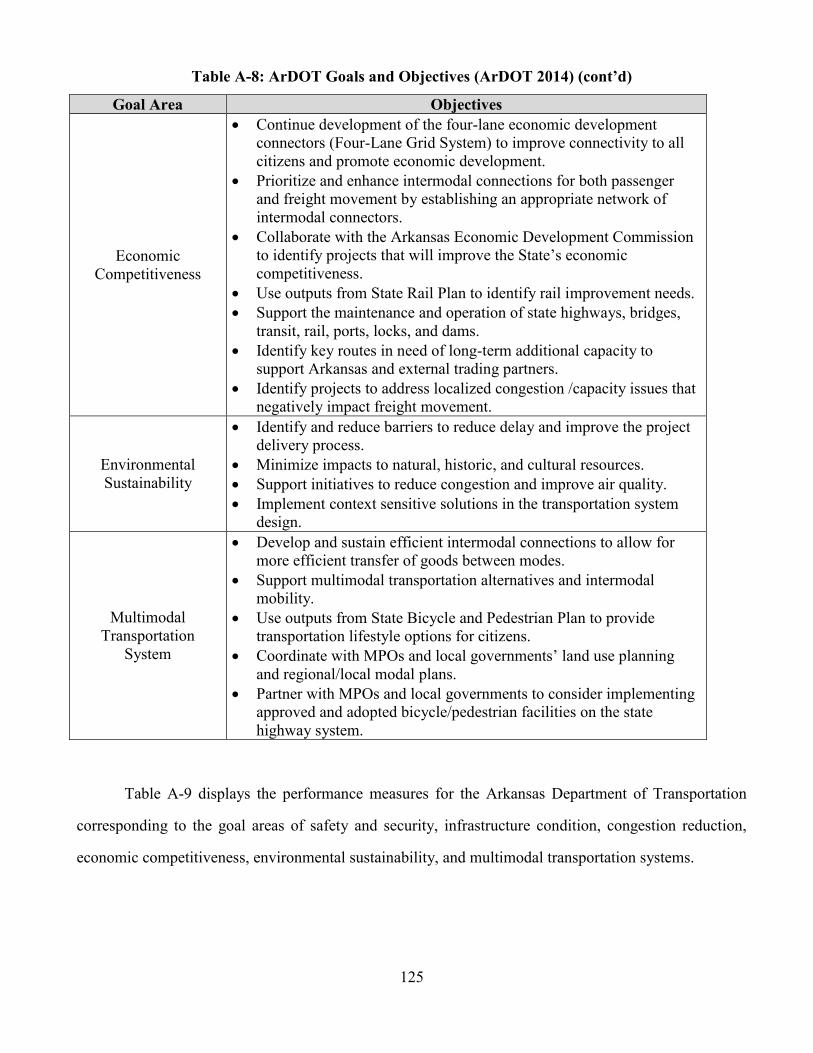
125
Table A-8: ArDOT Goals and Objectives (ArDOT 2014) (cont’d)
Goal Area Objectives
Economic
Competitiveness
Continue development of the four-lane economic development
connectors (Four-Lane Grid System) to improve connectivity to all
citizens and promote economic development.
Prioritize and enhance intermodal connections for both passenger
and freight movement by establishing an appropriate network of
intermodal connectors.
Collaborate with the Arkansas Economic Development Commission
to identify projects that will improve the State’s economic
competitiveness.
Use outputs from State Rail Plan to identify rail improvement needs.
Support the maintenance and operation of state highways, bridges,
transit, rail, ports, locks, and dams.
Identify key routes in need of long-term additional capacity to
support Arkansas and external trading partners.
Identify projects to address localized congestion /capacity issues that
negatively impact freight movement.
Environmental
Sustainability
Identify and reduce barriers to reduce delay and improve the project
delivery process.
Minimize impacts to natural, historic, and cultural resources.
Support initiatives to reduce congestion and improve air quality.
Implement context sensitive solutions in the transportation system
design.
Multimodal
Transportation
System
Develop and sustain efficient intermodal connections to allow for
more efficient transfer of goods between modes.
Support multimodal transportation alternatives and intermodal
mobility.
Use outputs from State Bicycle and Pedestrian Plan to provide
transportation lifestyle options for citizens.
Coordinate with MPOs and local governments’ land use planning
and regional/local modal plans.
Partner with MPOs and local governments to consider implementing
approved and adopted bicycle/pedestrian facilities on the state
highway system.
Table A-9 displays the performance measures for the Arkansas Department of Transportation
corresponding to the goal areas of safety and security, infrastructure condition, congestion reduction,
economic competitiveness, environmental sustainability, and multimodal transportation systems.

126
Table A-9: ArDOT Performance Measures (ArDOT 2017)
Goal Area Performance Measures
Safety and Security
Statewide number of fatalities
Statewide number of serious injuries
Fatalities/100 million VMT
Serious Injuries/100 million VMT
Statewide combined number of non-motorized fatalities and serious
injuries
Roadway Clearance Time (RCT)
Infrastructure
Condition
Percent of Bridge Deck Area on the NHS in Good Condition
Percent of Bridge Deck Area on the NHS in Poor Condition
Percent of Pavement on the Interstate in Good Condition
Percent of Pavement on the Non-Interstate NHS in Good Condition
Percent of Pavement on the Interstate in Poor Condition
Percent of Pavement on the Non-Interstate NHS in Poor Condition
Congestion Reduction
Percent of person-miles traveled on the Interstate system that are
reliable
Percent of person-miles traveled on the non-Interstate NHS that are
reliable
Percent change in tailpipe CO2 emissions on the NHS from calendar
year 2017
Economic
Competitiveness
Percentage of the Interstate system mileage providing for reliable
truck travel times or Truck Travel Time Reliability (TTTR) Index
(referred to as the Freight Reliability Measure)
Year-to-year change in statewide average job accessibility (separate
measures for auto and transit modes)
Environmental
Sustainability
Annual hours of peak-hour excessive delay per capita (the PHED
measure)
Percent of Non-SOV travel where SOV stands for single-occupancy
vehicle
Total emissions reduction
Multimodal
Transportation
System
Percent of revenue vehicles with a particular asset class that have
either met or exceeded their useful life benchmark (ULB)
DOTD GOALS, OBJECTIVES, AND PERFORMANCE MEASURES
Table A-10 shows the goals and objectives for the Louisiana Department of Transportation
corresponding to the goal areas of infrastructure preservation and maintenance, safety, economic
competitiveness, community development and enhancement, and environmental stewardship.

127
Table A-10: DOTD Goals and Objectives (DOTD 2015)
Goal Area Objectives
Infrastructure
Preservation and
Maintenance
Keep Louisiana’s state highway pavement, bridges, and highway
related assets in good condition.
Assist modal partners in achieving state-of-good-repair for aviation,
port, rail, transit, and navigable waterway infrastructure.
Assist local roadway departments in achieving state-of-good-repair
for locally owned roads and streets.
Safety
Reduce the number and rate of highway-related crashes, fatalities,
and serious injuries.
Reduce the number of pedestrian and bicycle crashes.
Assist modal partners in achieving safe and secure aviation, port,
rail, transit, and waterway performance.
Economic
Competitiveness
Improve the efficiency of freight transportation and the capacity of
freight related infrastructure throughout Louisiana.
Improve access to intermodal facilities and the efficiency of
intermodal transfers.
Provide predictable, reliable travel times throughout Louisiana.
Ensure small urban areas (5,000+ population) are well connected
with one another and with large urban employment centers.
Community
Development and
Enhancement
Cooperate with and support MPOs, state planning and development
districts, and local governments with the establishment and
refinement of land use, transportation, and community development
plans.
Increase options available to local governments to seek sustainable
revenue for local transportation needs.
Continue the Road Transfer Program as a voluntary program to
assist local governments in addressing local transportation needs.
Reduce barriers to state and local collaboration.
Enhance access to jobs for both urban and rural populations.
Improve modal options associated with supporting the economy and
quality of life regardless of age, disability, or income.
Identify methods to preserve the integrity and character of “town
centers” and preserve open space, or the appearance of open space,
between them.
Environmental
Stewardship
Minimize the environmental impacts of building, maintaining, and
operating Louisiana’s transportation system.
Comply with all federal and state environmental regulations
Table A-11 displays the performance measures for the Louisiana Department of Transportation
corresponding to the goal areas of infrastructure preservation and maintenance, safety, economic
competitiveness, community development and enhancement, and environmental stewardship.
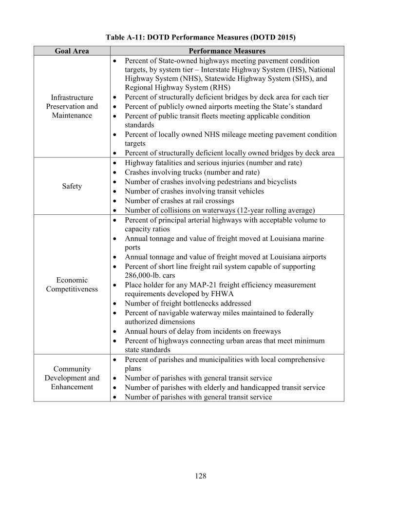
128
Table A-11: DOTD Performance Measures (DOTD 2015)
Goal Area Performance Measures
Infrastructure
Preservation and
Maintenance
Percent of State-owned highways meeting pavement condition
targets, by system tier – Interstate Highway System (IHS), National
Highway System (NHS), Statewide Highway System (SHS), and
Regional Highway System (RHS)
Percent of structurally deficient bridges by deck area for each tier
Percent of publicly owned airports meeting the State’s standard
Percent of public transit fleets meeting applicable condition
standards
Percent of locally owned NHS mileage meeting pavement condition
targets
Percent of structurally deficient locally owned bridges by deck area
Safety
Highway fatalities and serious injuries (number and rate)
Crashes involving trucks (number and rate)
Number of crashes involving pedestrians and bicyclists
Number of crashes involving transit vehicles
Number of crashes at rail crossings
Number of collisions on waterways (12-year rolling average)
Economic
Competitiveness
Percent of principal arterial highways with acceptable volume to
capacity ratios
Annual tonnage and value of freight moved at Louisiana marine
ports
Annual tonnage and value of freight moved at Louisiana airports
Percent of short line freight rail system capable of supporting
286,000-lb. cars
Place holder for any MAP-21 freight efficiency measurement
requirements developed by FHWA
Number of freight bottlenecks addressed
Percent of navigable waterway miles maintained to federally
authorized dimensions
Annual hours of delay from incidents on freeways
Percent of highways connecting urban areas that meet minimum
state standards
Community
Development and
Enhancement
Percent of parishes and municipalities with local comprehensive
plans
Number of parishes with general transit service
Number of parishes with elderly and handicapped transit service
Number of parishes with general transit service
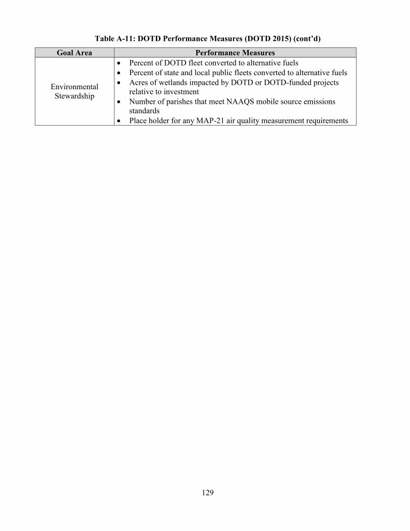
129
Table A-11: DOTD Performance Measures (DOTD 2015) (cont’d)
Goal Area Performance Measures
Environmental
Stewardship
Percent of DOTD fleet converted to alternative fuels
Percent of state and local public fleets converted to alternative fuels
Acres of wetlands impacted by DOTD or DOTD-funded projects
relative to investment
Number of parishes that meet NAAQS mobile source emissions
standards
Place holder for any MAP-21 air quality measurement requirements

130
Appendix B
Hurricane Data for the Sensitivity Analyses of Occurrence
Data used in the analyses conducted for the case studies in Chapter 5 are found in Table B-1.
This information includes the name of the hurricane, land fall date, hurricane wind speed, and wind
speed.

131
Table B-1: New Orleans Hurricane Data (NOAA 2017)
Name Date Category Wind Speed
(kn)
Wind Speed
(mph)
Allison 2001 TS 35 40.3
Babe 1977 TS 30 34.5
Betha 2002 TS 25 28.8
Beryl 1988 TS 45 51.8
Betsy 1965 H2 90 103.6
Bill 2003 TS 45 51.8
Bob 1979 H1 65 74.8
Bonnie 2010 TS 20 23.0
Brenda 1955 TS 55 63.3
Camille 1969 H5 150 172.6
Cindy 2005 TS 50 57.5
Danny 1997 H1 70 80.6
Elena 1985 H3 100 115.1
Esther 1957 TS 50 57.5
Fern 1971 TS 25 28.8
Florence 1988 TS 60 69.0
Gustav 2008 H2 90 103.6
Hermine 1998 TS 35 40.3
Hilda 1964 TS 60 69.0
Isaac 2012 H1 65 74.8
ISIDORE 2002 TS 55 63.3
JUAN 1985 TS 60 69.0
KATRINA 2005 H4 125 143.8
MATTHEW 2004 TS 30 34.5
UNNAMED 1855 H3 110 126.6
UNNAMED 1860 H3 100 115.1
UNNAMED 1860 H2 90 103.6
UNNAMED 1867 H2 90 103.6
UNNAMED 1869 H1 70 80.6
UNNAMED 1872 TS 50 57.5
UNNAMED 1877 H1 70 80.6
UNNAMED 1879 H3 110 126.6
UNNAMED 1879 TS 50 57.5
UNNAMED 1885 TS 60 69.0
UNNAMED 1887 H1 75 86.3
UNNAMED 1888 H2 85 97.8
UNNAMED 1889 H1 70 80.6

132
Table B-1: New Orleans Hurricane Data (NOAA 2017) (cont’d)
Name Date Category Wind Speed
(kn)
Wind Speed
(mph)
UNNAMED 1890 TS 50 57.5
UNNAMED 1892 TS 45 51.8
UNNAMED 1893 H1 70 80.6
UNNAMED 1893 H4 115 132.3
UNNAMED 1895 TS 50 57.5
UNNAMED 1900 TS 40 46.0
UNNAMED 1901 H1 75 86.3
UNNAMED 1905 TS 40 46.0
UNNAMED 1907 TS 40 46.0
UNNAMED 1912 TS 50 57.5
UNNAMED 1914 TS 35 40.3
UNNAMED 1915 H3 110 126.6
UNNAMED 1920 H2 85 97.8
UNNAMED 1923 TS 40 46.0
UNNAMED 1923 H1 70 80.6
UNNAMED 1923 TS 50 57.5
UNNAMED 1926 H3 100 115.1
UNNAMED 1926 TS 40 46.0
UNNAMED 1936 TS 40 46.0
UNNAMED 1936 TS 25 28.8
UNNAMED 1939 TS 45 51.8
UNNAMED 1944 TS 55 63.3
UNNAMED 1945 TS 30 34.5
UNNAMED 1947 TS 35 40.3
UNNAMED 1947 H2 95 109.3
UNNAMED 1948 H1 70 80.6
UNNAMED 1949 TS 50 57.5
UNNAMED 1955 TS 45 51.8
UNNAMED 1956 TS 50 57.5
UNNAMED 1971 TS 25 28.8
UNNAMED 1971 TS 25 28.8
UNNAMED 1975 TS 25 28.8
UNNAMED 1975 TS 25 28.8
UNNAMED 1977 TS 25 28.8
UNNAMED 1980 TS 20 23.0

133
Appendix C
Sample Calculations for the Risk of Failure of an Asset
This appendix contains sample calculations of a risk scenario from Chapter 5. This sample
calculations show how to apply the occurrence, severity, and risk priority calculation (RPN) equations
for a single scenario.
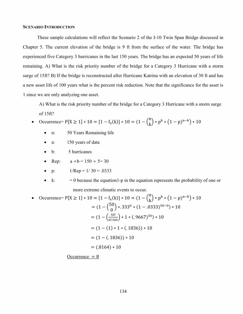
134
SCENARIO INTRODUCTION
These sample calculations will reflect the Scenario 2 of the I-10 Twin Span Bridge discussed in
Chapter 5. The current elevation of the bridge is 9 ft from the surface of the water. The bridge has
experienced five Category 3 hurricanes in the last 150 years. The bridge has an expected 50 years of life
remaining. A) What is the risk priority number of the bridge for a Category 3 Hurricane with a storm
surge of 15ft? B) If the bridge is reconstructed after Hurricane Katrina with an elevation of 30 ft and has
a new asset life of 100 years what is the percent risk reduction. Note that the significance for the asset is
1 since we are only analyzing one asset.
A) What is the risk priority number of the bridge for a Category 3 Hurricane with a storm surge
of 15ft?
Occurrence= P[X ≥ 1] ∗ 10 = [1 − fx(k)] ∗ 10 = (1 − (nk
) ∗ pk ∗ (1 − p)n−k) ∗ 10
n: 50 Years Remaining life
a: 150 years of data
b: 5 hurricanes
Rep: a ÷b = 150 ÷ 5= 30
p: 1/Rep = 1/ 30 = .0333
k: = 0 because the equation1-p in the equation represents the probability of one or
more extreme climatic events to occur.
Occurrence= P[X ≥ 1] ∗ 10 = [1 − fx(k)] ∗ 10 = (1 − (nk
) ∗ pk ∗ (1 − p)n−k) ∗ 10
= (1 − (500
) ∗. 3330 ∗ (1 − .0333)50−0) ∗ 10
= (1 − (50!
0!∗50!) ∗ 1 ∗ (. 9667)50) ∗ 10
= (1 − (1) ∗ 1 ∗ (. 1836)) ∗ 10
= (1 − (. 1836)) ∗ 10
= (.8164) ∗ 10
Occurrence = 8

135
Severity= P[Z < 0] ∗ (20 − Cp) = (1 − Φ(Z)) ∗ (20 − Cp)=(1 − Φ (ln (R
L))) ∗ (20 − Cp)
R: 9 ft
L: 15 ft
Cp: R – L = 9-15= -6ft
Severity= P[Z < 0] ∗ (20 − Cp) = (1 − Φ(Z)) ∗ (20 − Cp)=(1 − Φ (ln (R
L))) ∗ (20 − Cp)
=(1 − Φ (ln (9
15))) ∗ (20 − (−6))
=(1 − Φ(−.511)) ∗ (26)
=(1 − .305) ∗ (26)
=(.695) ∗ (26)
=18.077
Severity =10 Since higher than 10, Severity is maxed at 10.
RPN = Occurrence * Severity * Significance
Occurrence: 8
Severity: 10
Significance: 1
RPN = Occurrence * Severity * Significance
RPN = 8 * 10 * 1
RPN = 80
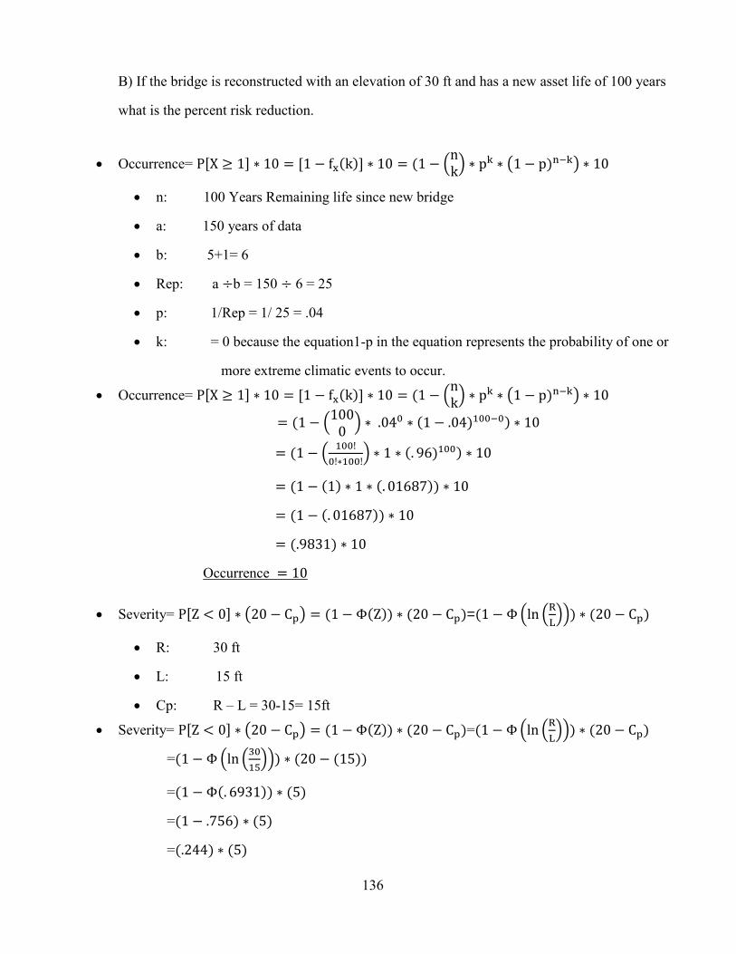
136
B) If the bridge is reconstructed with an elevation of 30 ft and has a new asset life of 100 years
what is the percent risk reduction.
Occurrence= P[X ≥ 1] ∗ 10 = [1 − fx(k)] ∗ 10 = (1 − (nk
) ∗ pk ∗ (1 − p)n−k) ∗ 10
n: 100 Years Remaining life since new bridge
a: 150 years of data
b: 5+1= 6
Rep: a ÷b = 150 ÷ 6 = 25
p: 1/Rep = 1/ 25 = .04
k: = 0 because the equation1-p in the equation represents the probability of one or
more extreme climatic events to occur.
Occurrence= P[X ≥ 1] ∗ 10 = [1 − fx(k)] ∗ 10 = (1 − (nk
) ∗ pk ∗ (1 − p)n−k) ∗ 10
= (1 − (100
0) ∗ .040 ∗ (1 − .04)100−0) ∗ 10
= (1 − (100!
0!∗100!) ∗ 1 ∗ (. 96)100) ∗ 10
= (1 − (1) ∗ 1 ∗ (. 01687)) ∗ 10
= (1 − (. 01687)) ∗ 10
= (.9831) ∗ 10
Occurrence = 10
Severity= P[Z < 0] ∗ (20 − Cp) = (1 − Φ(Z)) ∗ (20 − Cp)=(1 − Φ (ln (R
L))) ∗ (20 − Cp)
R: 30 ft
L: 15 ft
Cp: R – L = 30-15= 15ft
Severity= P[Z < 0] ∗ (20 − Cp) = (1 − Φ(Z)) ∗ (20 − Cp)=(1 − Φ (ln (R
L))) ∗ (20 − Cp)
=(1 − Φ (ln (30
15))) ∗ (20 − (15))
=(1 − Φ(. 6931)) ∗ (5)
=(1 − .756) ∗ (5)
=(.244) ∗ (5)
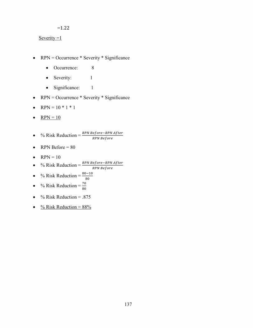
137
=1.22
Severity =1
RPN = Occurrence * Severity * Significance
Occurrence: 8
Severity: 1
Significance: 1
RPN = Occurrence * Severity * Significance
RPN = 10 * 1 * 1
RPN = 10
% Risk Reduction = 𝑅𝑃𝑁 𝐵𝑒𝑓𝑜𝑟𝑒−𝑅𝑃𝑁 𝐴𝑓𝑡𝑒𝑟
𝑅𝑃𝑁 𝐵𝑒𝑓𝑜𝑟𝑒
RPN Before = 80
RPN = 10
% Risk Reduction = 𝑅𝑃𝑁 𝐵𝑒𝑓𝑜𝑟𝑒−𝑅𝑃𝑁 𝐴𝑓𝑡𝑒𝑟
𝑅𝑃𝑁 𝐵𝑒𝑓𝑜𝑟𝑒
% Risk Reduction = 80−10
80
% Risk Reduction = 70
80
% Risk Reduction = .875
% Risk Reduction = 88%

138
Vita
Oscar Ortega was born in Fort Worth, Texas, on March 31, 1988. After finishing high school in
2006, he began his studies in Civil Engineering at the University of Texas at El Paso. After completing
his degree in 2010, he began his military service in the United States Army. In 2015, he finished his
service in the United States Army achieving the rank of Captain and began his graduate studies at the
University of Texas at El Paso. While conducting his graduate studies, he assisted in the editing of final
reports for granting agencies like TxDOT, NCHRP, and the El Paso Metropolitan Planning
Organization. The reports include “Quantification of the Impact of Roadway Conditions on Emissions”,
“Consequences of Delayed Maintenance of Highway Assets”, and “Development of a Sustainable Based
Methodology for Strategic Metropolitan Planning Based on MAP-21” respectively.
Permanent address: 12038 Royal Woods
El Paso, Texas, 79936
This thesis/dissertation was typed by Oscar Ortega.