IEEE TRANSACTIONS ON ROBOTICS, VOL. 35, NO. 3, JUNE 2019 725

A Switched Systems Approach to Path FollowingWith Intermittent State Feedback

Hsi-Yuan Chen , Zachary I. Bell , Patryk Deptula , and Warren E. Dixon , Fellow, IEEE

Abstract—Autonomous agents are often tasked with operat-ing in an area where feedback is unavailable. Inspired by suchapplications, this paper develops a novel switched system-basedcontrol method for uncertain nonlinear systems with temporaryloss-of-state feedback. To compensate for intermittent feedback,an observer is used while state feedback is available to reduce theestimation error, and a predictor is utilized to propagate the esti-mates while state feedback is unavailable. Based on the resultingsubsystems, maximum and minimum dwell time conditions are de-veloped via a Lyapunov-based switched systems analysis to relaxthe constraint of maintaining constant feedback. Using the dwelltime conditions, a switching trajectory is developed to enter andexit the feedback denied region in a manner that ensures that theoverall switched system remains stable. A scheme for designing aswitching trajectory with a smooth transition function is provided.Simulation and experimental results are presented to demonstratethe performance of control design.

Index Terms—Dwell time conditions, intermittent statefeedback, observer, predictor, switched systems theory.

I. INTRODUCTION

ACQUIRING state feedback is at the core of ensuring sta-bility in control designs. However, factors such as the task

definition, operating environment, or sensor modality can re-sult in temporary loss of feedback. For example, agents maybe required to limit communication during predefined timeframes or when traversing through certain regions. Motivatedby such factors, various path planning and control methods havebeen developed that seek to ensure uninterrupted feedback (cf.,[1]–[12]). Such results inherently constrain the trajectory orbehavior of a system. For instance, visual servoing applica-tions for nonholonomic systems can result in limited, sharp-angled, or nonsmooth trajectories to keep a target in the camerafield of view (FOV) as illustrated in results such as [13]–[15].Rather than trying to constrain the system to ensure continuous

Manuscript received November 25, 2018; accepted January 28, 2019. Date ofpublication March 20, 2019; date of current version May 31, 2019. This paperwas recommended for publication by Associate Editor Andreas Mueller uponevaluation of the reviewers’ comments. This work was supported in part by AirForce Office of Scientific Research (AFOSR) under Award FA9550-18-1-0109and in part by Naval Engineering Education Consortium (NEEC) under AwardN00174-18-1-0003. (Corresponding author: Hsi-Yuan Chen.)

The authors are with the Department of Mechanical and Aerospace Engi-neering, University of Florida, Gainesville, FL 32611 USA (e-mail:,hychen@ufl.edu; bellz121@ufl.edu; pdeptula@ufl.edu; wdixon@ufl.edu).

This paper has supplementary downloadable multimedia material available athttp://ieeexplore.ieee.org provided by the authors. This includes a video, whichshows a recording of the experiment with the motion of the quadcopter and theswitching trajectory projected on the floor. This material is 30.0 MB in size.

Color versions of one or more of the figures in this paper are available onlineat http://ieeexplore.ieee.org.

Digital Object Identifier 10.1109/TRO.2019.2899269

feedback availability, the approach in this paper leveragesswitched systems methods to achieve an objective despite in-termittent feedback. Some applications where this approachis useful include underwater operations that require vehiclesto resurface to acquire GPS, navigation within urban canyonswhere GPS is occluded, and exploration of areas where absolutepositioning systems have not been established (cf., [16]–[18]).

Solutions to relaxing the constant feedback constraint havebeen investigated. For example, methods to relax the require-ment of keeping landmarks in the FOV have been developed inresults such as [19] and [20]. In [19], multiple landmarks arelinked together by a daisy-chaining approach where new land-marks are mapped onto the initial world frame and are used toprovide state feedback when initial landmarks leave the FOV.Similar concepts were adopted in [20], where a wheeled mobilerobot is allowed to navigate around a landmark without con-stantly keeping it in the FOV by relating feature points in thebackground to the landmark and thus provide state feedback.Although the objective to eliminate the requirement of constantvisual on the landmark is achieved, state feedback is assumedto be available during periods when the landmark is outside theFOV. Such daisy-chaining approaches provide state feedbackin an ideal scenario, but the accuracy of the feedback may de-grade or even diverge in the presence of measurement noise anddisturbances in the dynamics.

Conventional approaches to the simultaneous localizationand mapping (SLAM) problem, such as the works in [21]–[23],use relationships between features or landmarks to estimatethe pose (i.e., position and orientation) of the sensor, usually amonocular camera, and simultaneously determine the positionof landmarks with respect to the world frame. Typically, afeature-rich environment with sufficient measurements are re-quired for SLAM methods to provide state estimation. However,a well-known drawback with SLAM algorithms is that withoutproper loop closures the estimates will drift over time due tothe accumulation of measurement noise (cf., [24], [25]). In thispaper, a state estimate dynamic model propagates the state esti-mate when feedback is not available, and no additional feedbackinformation is required. In SLAM applications, the feedbackregions defined in this paper can be represented as features orlandmarks with known absolute position. Hence, stability canbe achieved by closing the loop with respect to these knownfeatures or landmarks, and sufficient conditions may be derivedvia a Lyapunov-based analysis to ensure that the loop closuresare achieved before the state estimates degrade beyond a desiredthreshold.

1552-3098 © 2019 IEEE. Personal use is permitted, but republication/redistribution requires IEEE permission.See http://www.ieee.org/publications standards/publications/rights/index.html for more information.

726 IEEE TRANSACTIONS ON ROBOTICS, VOL. 35, NO. 3, JUNE 2019

Stability of systems that experience random state feed-back has been analyzed in previous literature. Typically, theintermittent loss of measurement is modeled as a randomBernoulli process with a known probability. Resulting trajec-tories are then analyzed in a probabilistic sense, where theexpected value of the estimation error is shown to convergeasymptotically, compared to the result in this paper which ex-amines the behavior of the actual tracking and estimation errors.

The networked control systems community has also examinedsystems with temporarily unavailable measurements. Resultssuch as [26]–[29] rely on a decision maker that is independentof the estimator or controller to determine when to broadcastsensor information. The objective in these results is to mini-mize the cost of network bandwidth by reducing the frequencyof data transmission. In [30]–[32], data loss is modeled as ran-dom missing outputs and noisy measurements. In each case,state estimates are propagated by a model of the controlled sys-tem during the periods when transmission is missing. On thecontrary, the availability of sensor information in this paper isdetermined by the region in which the actual states are located,which introduces a unique constraint of state-based feedbackavailability (i.e., even if a decision maker indicates that stateinformation should be made available, the agent has to leave itscurrent objective to return to a region where it can obtain stateinformation.) Therefore, sensor information is only availablewhen the states are inside a feedback region.

It is well-known that slow switching between stable subsys-tems may result in instability as explained in [33]. For slowswitching between stable subsystems, the underlying strategyfor proving stability involves developing switching conditionsto ensure the overall system is stable. If a common Lyapunovfunction exists for all subsystems such that the time deriva-tive of the Lyapunov function is upper bounded by a commonnegative definite function, the overall system is proven to bestable in [33]. For cases where a common Lyapunov functioncannot be determined, multiple subsystem-specific Lyapunovfunctions are used. In general, the overall Lyapunov functionis discontinuous and jumps may occur at switching interfaces.Therefore, the stability of such a system is achieved by placingswitching conditions on the subsystems to enforce a decrease inthe subsystem-specific Lyapunov functions between each suc-cessive activation of the respective subsystems. Typically, theserequirements manifest as (average) dwell time conditions whichspecifies the duration for which each subsystem must remainactive, as described in [33].

When a subset of the subsystems is unstable, a layer of com-plication is introduced into the analysis. A stability analysis isprovided in [34] for switched systems with stable and unstablelinear time-invariant subsystems, where an average dwell timecondition is developed. Similarly, in [35], Muller and Liberzondeveloped dwell time conditions for nonlinear switched systemswith exponentially stable and unstable subsystems. However,dwell time conditions typically require the stable subsystems tobe activated longer than the unstable subsystems, as indicated in[34]. In [36], Parikh et al. developed an observer to estimate thedepths of feature points in an image from a monocular cameraand use a predictor to propagate the state estimates when the fea-tures are occluded or outside the FOV. Based on the error system

formulation, the subsystem for the observer is stable, while thesubsystem for the predictor is unstable. An average dwell timecondition is developed to ensure the stability of the switchedsystem. However, the focus of [36] is the estimation of featuredepths and therefore, not on achieving a control objective whenfeedback is unavailable.

The development in this paper aims to achieve a path-following objective despite intermittent loss of feedback. Thenovelty of this result is guaranteeing the stability of following apath which lies outside a region with feedback while maximiz-ing the amount of time the agent spends in the feedback-deniedenvironment. Switched systems methods are used to develop astate estimator and predictor when state feedback is available ornot, respectively. Since switching occurs between a stable sub-system when feedback is available and an unstable subsystemwhen feedback is not available, dwell time conditions are devel-oped that determine the minimum time that the agent must bein the feedback region versus the maximum time the agent canbe in the feedback-denied region. Using these dwell time condi-tions, a switching trajectory is designed based on the dwell timeconditions that leads the agent in and out of the feedback-deniedregion so that the overall system remains stable. The most simi-lar result to this paper is in [37], which includes state predictionand control for a nonholonomic system moving around an ob-stacle. The goal in [37] is to regulate a nonholonomic vehicle toa set point in the presence of intermittent feedback. However,the difficulty of path following in the current paper arises whenthe system is outside the feedback region.

This paper is organized as follows. In Section II, the systemmodel is introduced. In Section III, the tracking and estimationobjective is given and the respective error systems are defined.Based on the error dynamics, a Lyapunov-based stability analy-sis for the resulting switched system is performed in Section Vto develop the dwell time conditions and to show the stabilityof the overall system. In Section VI, a strategy for designing aswitching trajectory is presented. A simulation is provided inSection VII and an experiment is provided in Section VIII todemonstrate the performance of the approach.

II. SYSTEM MODEL

Consider a dynamic system subject to an exogenousdisturbance as

x(t) = f(x(t), t) + v(t) + d(t) (1)

where x(t), x(t) ∈ Rn denote a generalized state and its timederivative, f : Rn × R → Rn denotes the locally Lipschitzdrift dynamics, v(t) ∈ Rn is the control input, and d(t) ∈ Rn

is the exogenous disturbance where n ∈ N and t ∈ R≥0 .Assumption 1: The Euclidean norm of the exogenous distur-

bance d(t) is bounded by ‖d(t)‖ ≤ d ∈ R≥0 .

III. STATE ESTIMATE AND CONTROL OBJECTIVE

In this paper, the overall objective is to achieve path follow-ing under intermittent loss of feedback. Specifically, a knownfeedback region is denoted as a closed set F ⊂ Rn , where thecomplement region where feedback is unavailable is denoted by

CHEN et al.: SWITCHED SYSTEMS APPROACH TO PATH FOLLOWING WITH INTERMITTENT STATE FEEDBACK 727

F c . That is, feedback is available when x(t) ∈ F and unavail-able when x(t) ∈ F c .

A desired path is denoted as xd ⊂ F c . It is clear that statefeedback is unavailable while attempting to follow xd , and hencethe system must return to the feedback regionF intermittently tomaintain stability. Therefore, a switching trajectory, denoted byxd(t) ∈ Rn , is designed to overlay xd as much as possible whileadhering to the subsequently developed dwell time constraints.To quantify the ability of the controller to track the switchingtrajectory, the tracking error e(t) ∈ Rn is defined as

e(t) � e1(t) + e2(t) (2)

where the estimate tracking error e1(t) ∈ Rn is defined as

e1(t) � x(t) − xd(t) (3)

and the state estimation error e2(t) ∈ Rn is defined as

e2(t) � x(t) − x(t) (4)

where x(t) ∈ Rn is the state estimate.Based on (3) and (4), the control objective is to ensure that

e1(t) and e2(t) converge, and therefore, e(t) will converge. Tofacilitate the subsequent development, let the composite errorvector be defined as z(t) � [eT

1 (t) eT2 (t)]T .

IV. CONTROLLER AND UPDATE LAW DESIGN

To facilitate the subsequent analysis, two subsystems are de-fined to indicate when the states are inside or outside the feed-back region. When x(t) ∈ F , an exponentially stable observercan be designed using various approaches (e.g., observers suchas [36], [38], and [39] could be used). The subsequent develop-ment is based on an observer update law designed as1

˙x(t) = f(x(t), t) + v(t) + vr (t) (5)

where vr (t) ∈ Rn is a high-frequency sliding-mode termdesigned as 2

vr (t) = k2e2(t) + dsgn(e2(t)) (6)

where k2 ∈ Rn×n is a constant, positive definite gain matrix.When x(t) ∈ F c , the state estimate is updated by a predictordesigned as

˙x(t) = f(x(t), t) + v(t). (7)

Since the state is required to transition between F and F c , aswitched systems analysis is used to investigate the stability ofthe overall switched system. To facilitate this analysis, the errorsystems for e1(t) and e2(t) are expressed as

e1(t) = f1p (xd(t), x(t), t) (8)

e2(t) = f2p (x(t), x(t), t) (9)

1Once x(t) ∈ F , a simple reset scheme (i.e., setting x(t) = x(t)) could beused. The reset scheme would eliminate the subsequently developed minimumdwell time for which x(t) is required to remain in the feedback region F .However, the subsequent development is based on the continued use of theobserver to illustrate a more general stability condition for systems that requirean observer or ˙x(t) ∈ L∞ ∀t.

2In cases where a piecewise-continuous controller is required, the robustifying

term in (5) may be designed as vr (t) = k2 e2 + d2

ε e2 , where ε ∈ R> 0 is adesign parameter.

where f1p , f2p : Rn × Rn × R≥0 → Rn , p ∈ {a, u}, a is anindex for subsystems with available feedback, and u is an indexfor subsystems when feedback is unavailable. Based on (8) andthe subsequent stability analysis, the controller is designed as

v(t) =

{˙xd(t) − f(x(t), t) − k1e1(t) − vr (t), p = a

˙xd(t) − f(x(t), t) − k1e1(t), p = u(10)

where ˙xd(t) ∈ Rn , and k1 ∈ Rn×n is a constant, positive def-inite gain matrix. By taking the time derivative of (3) and sub-stituting (5), (7), and (10) into the resulting expression, (8) canbe expressed as

e1(t) = −k1e1(t) ∀p. (11)

After taking the time derivative of (4) and substituting (1), (5),and (7) into the resulting expression, the family of systems in(9) can be expressed as

e2(t) =

⎧⎪⎨⎪⎩

f(x(t), t) − f(x(t), t) + d(t)

−dsgn(e2(t)) − k2e2(t) p = a

f(x(t), t) − f(x(t), t) + d(t) p = u

. (12)

V. SWITCHED SYSTEM ANALYSIS

To further facilitate the analysis for the switched system,let tai ∈ R≥0 denote the time of the ith instance when x(t)transitions from F c to F , and tui ∈ R>0 denote the time of theith instance when x(t) transitions from F to F c , for i ∈ N.The dwell time in the ith activation of the subsystems a and u isdefined as Δtai � tui − tai ∈ R>0 and Δtui � tai+1 − tui ∈ R>0 ,respectively. By Assumption 2 subsystem a is activated whent = 0, and consequently tui > tai ∀i ∈ N.

Assumption 2: The system is initialized in a feedback region(i.e., x(0) ∈ F).

To analyze the switched system, a common Lyapunov-likefunction is designed as

Vσ (z(t)) = V1(e1(t)) + V2(e2(t)) (13)

where the candidate Lyapunov functions for the tracking errorand the estimation error are selected, respectively, as

V1(e1(t)) =12eT

1 (t)e1(t) (14)

V2(e2(t)) =12eT

2 (t)e2(t). (15)

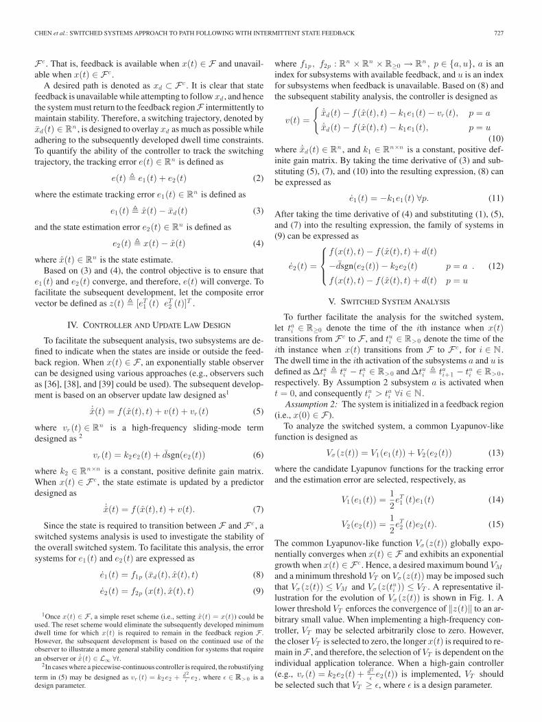
The common Lyapunov-like function Vσ (z(t)) globally expo-nentially converges when x(t) ∈ F and exhibits an exponentialgrowth when x(t) ∈ F c . Hence, a desired maximum bound VM

and a minimum threshold VT on Vσ (z(t)) may be imposed suchthat Vσ (z(t)) ≤ VM and Vσ (z(tui )) ≤ VT . A representative il-lustration for the evolution of Vσ (z(t)) is shown in Fig. 1. Alower threshold VT enforces the convergence of ‖z(t)‖ to an ar-bitrary small value. When implementing a high-frequency con-troller, VT may be selected arbitrarily close to zero. However,the closer VT is selected to zero, the longer x(t) is required to re-main inF , and therefore, the selection of VT is dependent on theindividual application tolerance. When a high-gain controller(e.g., vr (t) = k2e2(t) + d2

ε e2(t)) is implemented, VT shouldbe selected such that VT ≥ ε, where ε is a design parameter.

728 IEEE TRANSACTIONS ON ROBOTICS, VOL. 35, NO. 3, JUNE 2019

Fig. 1. Representative illustration for the evolution of Vσ during the interval[tai , tai+2 ].

Theorem 1: The composite error system trajectories ofthe switched system generated by the family of subsystemsdescribed by (11), (12), and a piecewise constant, right con-tinuous switching signal σ : [0,∞) → p ∈ {a, u} are globallyuniformly ultimately bounded provided the switching signalsatisfies the minimum feedback availability dwell time condition

Δtai ≥ −1λs

ln(

min(

VT

Vσ (z(tai )), 1))

(16)

and the maximum loss of feedback dwell time condition

Δtui ≤ 1λu

ln

(VM + d2

2λu

Vσ (z(tui )) + d2

2λu

)(17)

where λs and λu are subsequently defined known positiveconstants.

Proof: By taking the time derivative of (14) and substitutingfor (11) yields

V1(e1(t)) ≤ −2k1V1(e1(t)) ∀t (18)

where k1 is the minimum eigenvalue of k1 . By using (12), thetime derivative of (15) can be expressed as

V2(e2(t)) ≤{−2(k2 − c)V2(e2(t)), t ∈ [tai , tui )

λuV2(e2(t)) + 12 d2 , t ∈ [tui , tai+1)

(19)

where c ∈ R>0 is a Lipschitz constant, k2 > c ∈ R is theminimum eigenvalue of k2 , and λu � 2c + 1 ∈ R>0 .

From (18) and (19), the time derivative of the commonLyapunov-like function can be expressed as

Vσ (z(t)) ≤{−λsVσ (z(t)), t ∈ [tai , tui )

λuVσ (z(t)) + 12 d2 , t ∈ [tui , tai+1)

∀i ∈ N

(20)

where λs = 2min (k1 , (k2 − c)) ∈ R>0 . The solutions to (20)for the two subsystems are

Vσ (z(t)) ≤ Vσ (z(tai ))e−λs (t−tai ), t ∈ [tai , tui ) (21)

Vσ (z(t)) ≤ Vσ (z(tui ))eλu (t−tui )

− d2

2λu

(1 − eλu (t−tu

i ))

, t ∈ [tui , tai+1). (22)

The inequality in (21) indicates that ‖z(t)‖ ≤ ‖z(tai )‖e−

12 λs (t−ta

i ) , t ∈ [tai , tui ). The minimum threshold VT is selectedto enforce the convergence of ‖z(t)‖ to the desired threshold be-fore allowing x(t) to transition intoF c . This condition can be ex-pressed as Vσ (z(tai ))e−λs Δta

i ≤ VT , and therefore, the conditionin (16) is obtained after algebraic manipulation. If VT

Vσ (tai ) > 1,

the value of Vσ (tai ) is already below the threshold and thus, nominimum dwell time is required for the subsystem.

When t ∈ [tui , tai+1), the inequality in (22) indicates that

‖z‖ ≤√‖z(tui )‖2eλu (t−tu

i ) − d2

2λu(1 − eλu (t−tu

i )), and hence,the maximum bound VM is selected to limit the growth oferrors, where VM > VT . The maximum dwell time condi-tion for each of the ith unstable periods is expressed asVσ (z(tui ))eλu Δtu

i − d2

2λu(1 − eλu Δtu

i ) ≤ VM , and therefore, thecondition in (17) can be obtained.

Therefore, the composite error system trajectories generatedby (11) and (12) are globally uniformly ultimately bounded asdepicted in Fig. 1. �

VI. SWITCHING TRAJECTORY DESIGN

Since xd lies outside the feedback region, i.e., xd ⊂ F c ∀t,and cannot be followed for all time, the switching trajectoryxd(t) is designed to enable x(t) to follow xd to the extent pos-sible given the dwell time conditions in (16) and (17). A designchallenge for xd(t) is to ensure x(t) reenters F to satisfy thesufficient condition in (17). While x(t) transitions through F c ,e(t) may grow as indicated by (22), and this growth must be ac-counted for when designing xd(t). To facilitate the developmentof the switching trajectory xd(t), xb(t) ∈ Rn is defined as theclosest orthogonal projection of xd(t) on the boundary of F .

When the maximum dwell time condition is reached,‖e(t)‖ ≤ 2

√VM . This bound implies that there exists a set

B ={y ∈ Rn |‖y − xd(t)‖ ≤ 2

√VM

}such that x(t) ∈ B ∀t.

Therefore, the switching trajectory must penetrate a sufficientdistance into F to compensate for the error accumulation. Thedistance to compensate for error growth motivates the design ofa cushion that ensures the reentry of the actual states when themaximum dwell time is reached. To compensate for the potentialaccumulation of error, xd(t) must penetrate a sufficient distanceinto F , motivating the design of a cushion state xε(t) ∈ Rn as

xε(t) � xb(t) + Φ(t)

where Φ(t) ∈ Rn , such that ‖Φ(t)‖ ≥ 2√

VM and there exists acompact set A = {y ∈ Rn |‖y − xε(t)‖ ≤ ‖Φ(t)‖} such that Ais less than or equal to the inscribed ball of F in Rn . Therefore,the requirement of x(t) ∈ B ⊆ A ⊆ F can be satisfied if xσ (t)coincides with xε(t) when the maximum dwell time is reached.

CHEN et al.: SWITCHED SYSTEMS APPROACH TO PATH FOLLOWING WITH INTERMITTENT STATE FEEDBACK 729

A. Design Example

An example switching trajectory xd(t) can be developed uti-lizing a smootherstep function described in [40] to transitionsmoothly between xd and xε(t) while meeting the dwell timeconditions (see Remark 1). The smootherstep function is definedin [40] as

S(ρ) = 6ρ5 − 15ρ4 + 10ρ3 (23)

where ρ ∈ [0, 1] is the input parameter. Given the transitionfunction in (23), the switching trajectory is designed as

xd(t) �

⎧⎪⎪⎪⎪⎪⎪⎪⎨⎪⎪⎪⎪⎪⎪⎪⎩

H(S(ρa

i ), xb(t), xε(t)), tai ≤ t < tui

H(S(ρu1

i ), g (xd, t) , xb(t)), tui ≤ t < tu1

i

H(S(ρu2

i ), g (xd, t) , g (xd, t)), tu1

i ≤ t < tu2i

H(S(ρu3

i ), xε(t), g (xd, t)), tu2

i ≤ t < tu3i

(24)

where H (S(·), q (t) , r (t)) � S(·)q (t) + [1 − S(·)] r (t) forq(t), r(t) ∈ Rn , g : xd × R → Rn gives the desired state on xd

at time t, ρai , ρu1

i ρu2i , and ρu3

i are designed as ρai � t−ta

i

Δtai

and

ρuj+1i � t−(tu

i +∑ j

k = 0 pk Δtui )

pj + 1 Δtui

, j ∈ {0, 1, 2}, the weights used to

partition the maximum dwell time are denoted by pk ∈ [0, 1),and the corresponding partitions are denoted by tuj+1

i . The finalpartition tu3

i coincides with tai+1 . To avoid singularity in ρai and

to ensure a smooth and continuous switching trajectory, Δtaimust be arbitrarily lower bounded above zero (see Remark 2).

Remark 1: The switching trajectory is designed to compen-sate for the worst-case scenario where it must penetrate the en-tirety of the cushion to ensure x (t) enters F . However, if x (t)is able to reach F before the dwell time condition is reached,the agent may remain stationary for the entirety of the minimumdwell time. Other trajectories satisfying the dwell time condi-tions in Theorem 1 may also be implemented, such as the workin [37].

Remark 2: Lower bounding Δtai by an arbitrary value α ∈R>0 does not violate Theorem 1 since the system is allowed toremain in the feedback region longer than the minimum dwelltime, implying that Δtai ≤ α ≤ (t − tai ) holds. Other trajectorydesigns may not require Δtai to be lower bounded.

VII. SIMULATION

A simulation is performed to illustrate the performance ofthe controller, given the intermittent loss-of-state feedback.Based on the system model given in (1), f(x(t), t) is se-lected as f(x(t), t) = Ax where A = 0.5I3 , and d(t) is drawnfrom a uniform distribution between [0, 0.06] m/s. The initialstates and estimates are selected as x(0) = [0.1 m 0.2 m 0 rad]and x(0) = [0.2 m 0.3 m π

6 rad ]. The observer and the controllergains were selected as k1 = 3I3 and k2 = 3I3 , respectively.The desired upper bound and lower threshold for the com-posite error ‖z(t)‖ are selected as 0.9 and 0.02 m, respec-tively. Based on the desired error bound and threshold, the

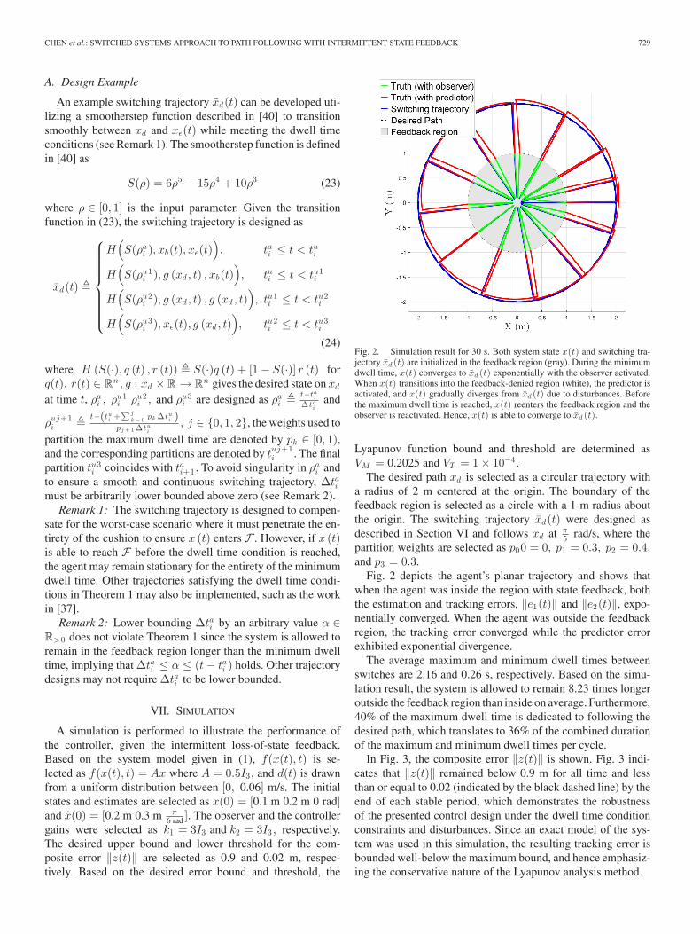
Fig. 2. Simulation result for 30 s. Both system state x(t) and switching tra-jectory xd (t) are initialized in the feedback region (gray). During the minimumdwell time, x(t) converges to xd (t) exponentially with the observer activated.When x(t) transitions into the feedback-denied region (white), the predictor isactivated, and x(t) gradually diverges from xd (t) due to disturbances. Beforethe maximum dwell time is reached, x(t) reenters the feedback region and theobserver is reactivated. Hence, x(t) is able to converge to xd (t).

Lyapunov function bound and threshold are determined asVM = 0.2025 and VT = 1 × 10−4 .

The desired path xd is selected as a circular trajectory witha radius of 2 m centered at the origin. The boundary of thefeedback region is selected as a circle with a 1-m radius aboutthe origin. The switching trajectory xd(t) were designed asdescribed in Section VI and follows xd at π

5 rad/s, where thepartition weights are selected as p00 = 0, p1 = 0.3, p2 = 0.4,and p3 = 0.3.

Fig. 2 depicts the agent’s planar trajectory and shows thatwhen the agent was inside the region with state feedback, boththe estimation and tracking errors, ‖e1(t)‖ and ‖e2(t)‖, expo-nentially converged. When the agent was outside the feedbackregion, the tracking error converged while the predictor errorexhibited exponential divergence.

The average maximum and minimum dwell times betweenswitches are 2.16 and 0.26 s, respectively. Based on the simu-lation result, the system is allowed to remain 8.23 times longeroutside the feedback region than inside on average. Furthermore,40% of the maximum dwell time is dedicated to following thedesired path, which translates to 36% of the combined durationof the maximum and minimum dwell times per cycle.

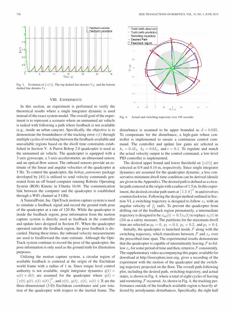
In Fig. 3, the composite error ‖z(t)‖ is shown. Fig. 3 indi-cates that ‖z(t)‖ remained below 0.9 m for all time and lessthan or equal to 0.02 (indicated by the black dashed line) by theend of each stable period, which demonstrates the robustnessof the presented control design under the dwell time conditionconstraints and disturbances. Since an exact model of the sys-tem was used in this simulation, the resulting tracking error isbounded well-below the maximum bound, and hence emphasiz-ing the conservative nature of the Lyapunov analysis method.

730 IEEE TRANSACTIONS ON ROBOTICS, VOL. 35, NO. 3, JUNE 2019

Fig. 3. Evolution of ‖z(t)‖. The top dashed line denotes VM and the bottomdashed line denotes VT .

VIII. EXPERIMENTS

In this section, an experiment is performed to verify thetheoretical results where a single integrator dynamic is usedinstead of the exact system model. The overall goal of the exper-iment is to represent a scenario where an unmanned air vehicleis tasked with following a path where feedback is not available(e.g., inside an urban canyon). Specifically, the objective is todemonstrate the boundedness of the tracking error e(t) throughmultiple cycles of switching between the feedback-available andunavailable regions based on the dwell time constraints estab-lished in Section V. A Parrot Bebop 2.0 quadcopter is used asthe unmanned air vehicle. The quadcopter is equipped with a3-axis gyroscope, a 3-axis accelerometer, an ultrasound sensor,and an optical-flow sensor. The onboard sensors provide an es-timate of the linear and angular velocities of the quadcopter at5 Hz. To control the quadcopter, the bebop_autonomy packagedeveloped by [41] is utilized to send velocity commands gen-erated from an off board computer running Robotic OperatingSystem (ROS) Kinetic in Ubuntu 16.04. The communicationlink between the computer and the quadcopter is establishedthrough a WiFi channel at 5 GHz.

A NaturalPoint, Inc. OptiTrack motion capture system is usedto simulate a feedback signal and record the ground truth poseof the quadcopter at a rate of 120 Hz. While the quadcopter isinside the feedback region, pose information from the motioncapture system is directly used as feedback in the controllerand update laws designed in Section IV. When the quadcopteroperated outside the feedback region, the pose feedback is dis-carded. During these times, the onboard velocity measurementsare used to feedforward the state estimate. Although the Opti-Track system continue to record the pose of the quadcopter, thepose information is only used as the ground truth for illustrationpurposes.

Utilizing the motion capture system, a circular region ofavailable feedback is centered at the origin of the Euclideanworld frame with a radius of 1 m. Since torque level controlauthority is not available, single integrator dynamics q(t) =u(t) + d(t) are assumed for the quadcopter where q(t) =[x(t) y(t) z(t) α(t)

]T, and x(t), y(t), z(t), α(t) ∈ R are the

three-dimensional (3-D) Euclidean coordinates and yaw rota-tion of the quadcopter with respect to the inertial frame. The

Fig. 4. Actual and switching trajectory over 185 seconds.

disturbance is assumed to be upper bounded as d = 0.035.To compensate for the disturbance, a high-gain robust con-troller is implemented to ensure a continuous control com-mand. The controller and update law gains are selected ask1 = 0.4I4 , k2 = 0.6I4 , and ε = 0.1. To regulate and matchthe actual velocity output to the control command, a low-levelPID controller is implemented.

The desired upper bound and lower threshold on ‖z(t)‖ areselected as 0.9 and 0.14 m, respectively. Since single integratordynamics are assumed for the quadcopter dynamic, a less con-servative minimum dwell time condition can be derived (detailsare given in the Appendix). The desired path is defined as a circu-lar path centered at the origin with a radius of 1.5 m. In this exper-iment, the desired circular path starts at

[1.5 0

]Tm and revolves

counterclockwise. Following the design method outlined in Sec-tion VI, a switching trajectory is designed to follow xd with anangular velocity of π

15 rad/s. To prevent the quadcopter fromdrifting out of the feedback region prematurely, a intermediatetrajectory is designed to be xint(t) = 0.7xb(t) to replace xb(t) in(24) as a safety measure. The partitions for the maximum dwelltime are selected as p0 = 0, p1 = 0.4, p2 = 0.2, and p3 = 0.4.

Initially, the quadcopter is launched inside F along with theswitching trajectory, which transitions between F and xd overthe prescribed time span. The experimental results demonstratethat the quadcopter is capable of intermittently leaving F to fol-low xd for some period of time and then, return toF consistently.The supplementary video accompanying this paper, available fordownload at http://ieeexplore.ieee.org, gives a recording of theexperiment with the motion of the quadcopter and the switch-ing trajectory projected on the floor. The overall path-followingplot, including the desired path, switching trajectory, and actualstates, is shown in Fig. 4, where a total of eight cycles of leavingand reentering F occurred. As shown in Fig. 4, the tracking per-formance outside of the feedback-available region is heavily af-fected by aerodynamic disturbances. Specifically, the right half

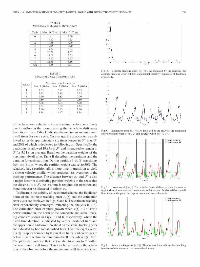
CHEN et al.: SWITCHED SYSTEMS APPROACH TO PATH FOLLOWING WITH INTERMITTENT STATE FEEDBACK 731

TABLE IMINIMUM AND MAXIMUM DWELL TIMES

TABLE IIMAXIMUM DWELL TIME PARTITIONS

of the trajectory exhibits a worse tracking performance likelydue to airflow in the room, causing the vehicle to drift awayfrom its estimate. Table I indicates the maximum and minimumdwell times for each cycle. On average, the quadcopter was al-lowed to reside approximately six times longer in F c than F ,and 20% of which is dedicated to following xd . Specifically, thequadcopter is allowed 19.85 s in F c and is required to remain inF for 3.31 s on average. Based on the partition weights of themaximum dwell time, Table II describes the partitions and theduration for each partition. During partition 1, xd(t) transitionsfrom xb(t) to xd where the partition weight was set to 50%. Therelatively large partition allots more time in transition to yielda slower velocity profile, which produces less overshoot in thetracking performance. The distance between xd and F is alsoa major factor in distributing partition weights in the sense thatthe closer xd is to F , the less time is required for transition andmore time can be allocated to follow xd .

To illustrate the stability of the control scheme, the Euclideannorm of the estimate tracking error e1(t) and the estimationerror e2(t) are displayed in Figs. 5 and 6. The estimate trackingerror exponentially converges, reflecting the analysis in (18).The estimation error exhibits growth when x(t) ∈ F c . For abetter illustration, the norm of the composite and actual track-ing error are shown in Figs. 7 and 8, respectively, where thedwell time duration is indicated by vertical dash-dot lines andthe upper bound and lower threshold on the actual tracking errorare indicated by horizontal dashed lines. Over the eight cycles,‖z(t)‖ is upper bounded by 0.9 m at all times, and converges tobelow 0.14 m within the minimum dwell time when x(t) ∈ F .The plots also indicate that x(t) is able to return to F withinthe maximum dwell times. This can be verified by the activa-tion of the observer before the maximum dwell time is reached

Fig. 5. Estimate tracking error ‖e1 (t)‖. As indicated by the analysis, theestimate tracking error exhibits exponential stability regardless of feedbackavailability.

Fig. 6. Estimation error ‖e2 (t)‖. As indicated by the analysis, the estimationerror converges when x(t) ∈ F and diverges when x(t) ∈ F c .

Fig. 7. Evolution of ‖z(t)‖. The dash-dot (vertical) lines indicate the switch-ing interface of minimum and maximum dwell times, and the dashed (horizontal)lines indicate the prescribed upper bound and lower threshold.

Fig. 8. Actual tracking error ‖e(t)‖. The dash-dot lines indicate the switchinginterface of minimum and maximum dwell times.

732 IEEE TRANSACTIONS ON ROBOTICS, VOL. 35, NO. 3, JUNE 2019

Fig. 9. Evolution of Vσ (t). The dotted (vertical) lines indicate the time in-stants when the quadcopter crossed the feedback region boundary. The dashed(horizontal) lines indicate the prescribed VM and VT for Vσ .

for every cycle. In Fig. 9, the evolution of Vσ is shown alongwith the calculated VM and VT as indicated by the horizontaldashed lines. As expected, the Lyapunov-like function Vσ is up-per bounded below VM for all times and converges below VT

within the minimum dwell times. Based on Figs. 8 and 9, thecontroller and update laws developed in Section IV demonstraterobustness towards disturbances and a simple assumed dynamicmodel. Hence, the trajectory design scheme provided in Sec-tion VI is able to generate a switching signal σ(t) that satisfiedthe dwell time conditions developed in Section V and, therefore,verifying the claim in Theorem 1.

IX. CONCLUSION

In this paper, a novel method that utilizes a switched systemsapproach to ensure path-following stability under intermittentstate feedback was presented. The presented method relievedthe requirement of state feedback at all times. State estimateswere used in the tracking control to compensate for the intermit-tence of state feedback. A Lyapunov-based switched systemsanalysis was used to develop maximum and minimum dwelltime conditions to guarantee stability of the overall system. Thedwell time conditions allowed the desired path to be completelyoutside the feedback region, and a switching trajectory wasdesigned to bring the states back into the feedback regionbefore the error growth exceeded a defined threshold. Thecandidate switching trajectory switched between the desiredpath and the feedback region using smootherstep transitionfunctions. A simulation and an experiment were performed toillustrate the robustness of the control and trajectory design.Less conservative analysis methods were motivated for futurework as a means to reduce the conservative nature of the dwelltime conditions in this paper. In addition, future research willfocus on the development of an approximate optimal control ap-proach using adaptive dynamic programming concepts to yieldapproximately optimal results. Further efforts will also examinecases where the feedback region is time varying or unknown.

APPENDIX

When using single integrator dynamics x(t) = u + d(t),the resulting estimation error dynamics for the unstable sub-system is ‖e2(t)‖ ≤ d, and the corresponding Lyapunov-like

function derivative is Vσ (t) ≤ d‖e2(t)‖. By solving the ordi-nary differential equation for e2(t), the estimation error e2(t)exhibits a linear growth that can be bounded as e2(t) ≤ e2(tui ) +d(t − tui ). After substituting in the linear bound on e2(t), itfollows that Vσ (t) ≤ d‖e2(tui )‖ + d2(t − tui ), and solving theordinary differential equation yields Vσ (t) ≤ 1

2 d2 (t − tui ) 2 +d‖e2(tui )‖ (t − tui ) + Vσ (z(tui )). After imposing Vσ (t) ≤ VM

as the upper bound constraint, the maximum dwell time can bederived by solving the quadratic equation and taking the positiveroot as

Δtui ≤(√‖e2(tui )‖2 − 2 (Vσ (z(tui )) − VM ) − ‖e2(tui )‖

)d

.

ACKNOWLEDGMENT

Any opinions, findings and conclusions, or recommendationsexpressed in this material are those of the author(s) and do notnecessarily reflect the views of the sponsoring agency.

REFERENCES

[1] N. Gans, S. Hutchinson, and P. Corke, “Performance tests for visual servocontrol systems, with application to partitioned approaches to visual servocontrol,” Int. J. Rob. Res., vol. 22, no. 10, pp. 955–981, 2003.

[2] S. Hutchinson, G. Hager, and P. Corke, “A tutorial on visual servo control,”IEEE Trans. Robot. Autom., vol. 12, no. 5, pp. 651–670, Oct. 1996.

[3] N. Gans, G. Hu, K. Nagarajan, and W. E. Dixon, “Keeping multiplemoving targets in the field of view of a mobile camera,” IEEE Trans.Robot. Autom., vol. 27, no. 4, pp. 822–828, Aug. 2011.

[4] N. Gans, G. Hu, J. Shen, Y. Zhang, and W. E. Dixon, “Adaptive visual servocontrol to simultaneously stabilize image and pose error,” Mechatronics,vol. 22, no. 4, pp. 410–422, 2012.

[5] G. Hu, N. Gans, and W. E. Dixon, “Quaternion-based visual servo controlin the presence of camera calibration error,” Int. J. Robust NonlinearControl, vol. 20, no. 5, pp. 489–503, 2010.

[6] G. Hu, N. Gans, N. Fitz-Coy, and W. E. Dixon, “Adaptive homography-based visual servo tracking control via a quaternion formulation,” IEEETrans. Control Syst. Technol., vol. 18, no. 1, pp. 128–135, Jan. 2010.

[7] G. Hu et al., “Homography-based visual servo control with imperfectcamera calibration,” IEEE Trans. Autom. Control, vol. 54, no. 6, pp. 1318–1324, Jun. 2009.

[8] J. Chen, D. M. Dawson, W. E. Dixon, and V. Chitrakaran, “Navigationfunction-based visual servo control,” Automatica, vol. 43, pp. 1165–1177,2007.

[9] J. Chen, D. M. Dawson, W. E. Dixon, and A. Behal, “Adaptivehomography-based visual servo tracking for fixed and camera-in-handconfigurations,” IEEE Trans. Control Syst. Technol., vol. 13, no. 5,pp. 814–825, Sep. 2005.

[10] G. Palmieri, M. Palpacelli, M. Battistelli, and M. Callegari, “A comparisonbetween position-based and image-based dynamic visual servoings in thecontrol of a translating parallel manipulator,” J. Robot., vol. 2012, 2012,Art. no. 103954.

[11] N. Gans and S. Hutchinson, “Stable visual servoing through hybridswitched-system control,” IEEE Trans. Robot., vol. 23, no. 3, pp. 530–540, Jun. 2007.

[12] G. Chesi and A. Vicino, “Visual servoing for large camera displacements,”IEEE Trans. Robot. Autom., vol. 20, no. 4, pp. 724–735, Aug. 2004.

[13] N. R. Gans and S. A. Hutchinson, “A stable vision-based control schemefor nonholonomic vehicles to keep a landmark in the field of view,” inProc. IEEE Int. Conf. Robot. Autom., Roma, Italy, 2007, pp. 2196–2201.

[14] G. L. Mariottini, G. Oriolo, and D. Prattichizzo, “Image-based visualservoing for nonholonomic mobile robots using epipolar geometry,” IEEETrans. Robot., vol. 23, no. 1, pp. 87–100, Feb. 2007.

[15] G. Lopez-Nicolas, N. R. Gans, S. Bhattacharya, C. Sagues, J. J.Guerrero, and S. Hutchinson, “Homography-based control scheme formobile robots with nonholonomic and field-of-view constraints,” IEEETrans. Syst., Man, Cybern., vol. 40, no. 4, pp. 1115–1127, Aug. 2010.

[16] G. Conte, G. de Capua, and D. Scaradozzi, “Designing the NGC system ofa small ASV for tracking underwater targets,” Robot. Auton. Syst., vol. 76,no. C, pp. 46–57, Feb. 2016.

CHEN et al.: SWITCHED SYSTEMS APPROACH TO PATH FOLLOWING WITH INTERMITTENT STATE FEEDBACK 733

[17] K. Tanakitkorn, P. A. Wilson, S. R. Turnock, and A. B. Phillips, “Slidingmode heading control of an overactuated, hover-capable autonomous un-derwater vehicle with experimental verification,” J. Field Robot., vol. 35,no. 3, pp. 396–415, 2018.

[18] L. Jianfang, Z. Hao, and G. Jingli, “A novel fast target tracking methodfor UAV aerial image,” Open Phys., vol. 15, Jun. 2017, Art. no. 46.

[19] S. S. Mehta, G. Hu, A. P. Dani, and W. E. Dixon, “Multireference vi-sual servo control of an unmanned ground vehicle,” in Proc. AIAA Guid.Navigat. Control Conf., Honolulu, Hawaii, Aug. 2008.

[20] B. Jia and S. Liu, “Switched visual servo control of nonholonomic mo-bile robots with field-of-view constraints based on homography,” ControlTheory Technol., vol. 13, no. 4, pp. 311–320, 2015.

[21] G. Klein and D. Murray, “Parallel tracking and mapping for small ARworkspaces,” in Proc. IEEE ACM Int. Symp. Mixed Augmented Reality,2007, pp. 225–234.

[22] A. J. Davison, I. D. Reid, N. D. Molton, and O. Stasse, “MonoSLAM:Real-time single camera SLAM,” IEEE Trans. Pattern Anal. Mach. Intell.,vol. 29, no. 6, pp. 1052–1067, Jun. 2007.

[23] D. Cremers, “Direct methods for 3-D reconstruction and visual slam,” inProc. IEEE IAPR Int. Conf. Mach. Vis. Appl., 2017, pp. 34–38.

[24] B. Williams, M. Cummins, J. Neira, P. Newman, I. Reid, and J. Tardos,“A comparison of loop closing techniques in monocular SLAM,” Robot.Auton. Syst., vol. 57, no. 12, pp. 1188–1197, 2009.

[25] C. Cadena et al., “Past, present, and future of simultaneous localizationand mapping: Towards the robust-perception age,” IEEE Trans. Robot.,vol. 32, no. 6, pp. 1309–1332, Dec. 2016.

[26] E. Garcia and P. J. Antsaklis, “Adaptive stabilization of model-basednetworked control systems,” in Proc. Amer. Control Conf., San Francisco,CA, USA, 2011, pp. 1094–1099.

[27] S. S. Mehta, W. MacKunis, S. Subramanian, E. L. Pasiliao, and J. W.Curtis, “Stabilizing a nonlinear model-based networked control systemwith communication constraints,” in Proc. Amer. Control Conf., Washing-ton, DC, USA, 2013, pp. 1570–1577.

[28] E. Garcia and P. J. Antsaklis, “Model-based event-triggered control forsystems with quantization and time-varying network delays,” IEEE Trans.Autom. Control, vol. 58, no. 2, pp. 422–434, Feb. 2013.

[29] M. J. McCourt, E. Garcia, and P. J. Antsaklis, “Model-based event-triggered control of nonlinear dissipative systems,” in Proc. Amer. ControlConf., Portland, OR, USA, 2014, pp. 5355–5360.

[30] N. E. Leonard and A. Olshevsky, “Cooperative learning in multiagentsystems from intermittent measurements,” in Proc. IEEE Conf. Decis.Control, Florence, Italy, 2013, pp. 7492–7497.

[31] J. Liang, Z. Wang, and X. Liu, “Distributed state estimation for discrete-time sensor networks with randomly varying nonlinearities and missingmeasurements,” IEEE Trans. Neural Netw., vol. 22, no. 3, pp. 486–496,Mar. 2011.

[32] Y. Shi, H. Fang, and M. Yan, “Kalman filter-based adaptive control fornetworked systems with unknown parameters and randomly missing out-puts,” Int. J. Robust Nonlinear Control, vol. 19, no. 18, pp. 1976–1992,Dec. 2009.

[33] D. Liberzon, Switching in Systems and Control. Basel, Switzerland:Birkhauser, 2003.

[34] G. Zhai, B. Hu, K. Yasuda, and A. N. Michel, “Stability analysis ofswitched systems with stable and unstable subsystems: An average dwelltime approach,” Int. J. Syst. Sci., vol. 32, no. 8, pp. 1055–1061, Nov. 2001.

[35] M. A. Muller and D. Liberzon, “Input/output-to-state stability and state-norm estimators for switched nonlinear systems,” Automatica, vol. 48,no. 9, pp. 2029–2039, 2012.

[36] A. Parikh, T.-H. Cheng, H.-Y. Chen, and W. E. Dixon, “A switched systemsframework for guaranteed convergence of image-based observers withintermittent measurements,” IEEE Trans. Robot., vol. 33, no. 2, pp. 266–280, Apr. 2017.

[37] H.-Y. Chen, Z. I. Bell, R. Licitra, and W. E. Dixon, “Switched systemsapproach to vision-based tracking control of wheeled mobile robots,” inProc. IEEE Conf. Decis. Control, 2017, pp. 4902–4907.

[38] A. Dani, N. Fischer, Z. Kan, and W. E. Dixon, “Globally exponentiallystable observer for vision-based range estimation,” Mechatronics, vol. 22,no. 4, Special Issue on Visual Servoing, pp. 381–389, 2012.

[39] Z. I. Bell, H.-Y. Chen, A. Parikh, and W. E. Dixon, “Single scene andpath reconstruction with a monocular camera using integral concurrentlearning,” in Proc. IEEE Conf. Decis. Control, 2017, pp. 3670–3675.

[40] D. S. Ebert, Texturing & Modeling: A Procedural Approach. Burlington,MA, USA: Morgan Kaufmann, 2003.

[41] bebop_Autonomy Library. Accessed: Mar. 20, 2018. [Online]. Available:http://bebop-autonomy.readthedocs.io

Hsi-Yuan (Steven) Chen received the Ph.D. degreein mechanical engineering from the Department ofMechanical and Aerospace Engineering, Universityof Florida, Gainesville, FL, USA, in 2018.

He is experienced in computer vision-based stateestimation and Lyapunov-based control techniquesfor uncertain nonlinear systems. His main researchinterest includes the development of state-of-the-artcontrol methods for autonomous vehicles.

Zachary Bell received the B.S. degree in mechani-cal engineering with a minor in electrical engineer-ing and the M.S. degree in mechanical engineeringin 2015 and 2017, respectively, from the Universityof Florida, Gainesville, FL, USA, where is currentlyworking toward the Ph.D. degree in mechanical en-gineering under the supervision of Dr. Warren Dixonwith the Nonlinear Controls and Robotics Group.

His research interests include Lyapunov-based es-timation and control theory, visual estimation, simul-taneous localization and mapping, and mechanicaldesign.

Dr. Bell is the recipient of the Science, Mathematics, and Research forTransformation (SMART) Scholarship, an award sponsored by the Departmentof Defense, in 2018.

Patryk Deptula received the B.Sc. degree in mechan-ical engineering and a mathematics minor (Hons.),from Central Connecticut State University (CCSU),New Britain, CT, USA, in 2014, working on researchrelated to hybrid propellant rocket engines. He is cur-rently working toward the Ph.D. degree in mechani-cal engineering under the supervision of Dr. WarrenDixon, working on nonlinear controls and autonomy,with a focus on learning-based and adaptive controlin a variety of applications.

After graduating, he worked as an Engineer withthe Control and Diagnostic Systems (DSC) Group, Belcan Corporation, wherehe analyzed aircraft engine software. His research interests include, but arenot limited to, multiagent systems, human-machine interaction, and roboticsapplied to a variety of fields.

Warren Dixon received the Ph.D. degree in elec-trical engineering from the Department of Electri-cal and Computer Engineering, Clemson University,Clemson, SC, USA, in 2000.

He worked as a Research Staff Member and Eu-gene P. Wigner Fellow at Oak Ridge National Lab-oratory (ORNL) till 2004, when he joined the Uni-versity of Florida in the Mechanical and AerospaceEngineering Department, where he is an Ebaugh Pro-fessor. His main research interest includes the devel-opment and application of Lyapunov-based control

techniques for uncertain nonlinear systems.Dr. Dixon is the recipient of the 2009 and 2015 American Automatic Control

Council (AACC) O. Hugo Schuck (Best Paper) Award, the 2013 Fred EllersickAward for Best Overall MILCOM Paper, the 2011 American Society of Mechan-ical Engineers (ASME) Dynamics Systems and Control Division OutstandingYoung Investigator Award, and the 2006 IEEE Robotics and Automation So-ciety (RAS) Early Academic Career Award. He was awarded the Air ForceCommander’s Public Service Award (2016) for his contributions to the U.S. AirForce Science Advisory Board. He is currently or formerly an Associate Editorfor the ASME Journal of Journal of Dynamic Systems, Measurement and Con-trol, Automatica, IEEE CONTROL SYSTEMS, IEEE TRANSACTIONS ON SYSTEMS

MAN AND CYBERNETICS: PART B CYBERNETICS, and the International Journalof Robust and Nonlinear Control. He is an ASME Fellow.