Embed Size (px)
Citation preview

A System Dynamics Energy Model for a Sustainable
Transportation System
Stefano Armenia(1)
, Fabrizio Baldoni(2)
, Diego Falsini(3)
, Emanuele Taibi(4)
(1)“Sapienza” University of Rome, CATTID, P.le Aldo Moro, 5 - 00185 Rome (Italy),
(2)ENI S.p.A., Strategies and Development Dept, P.le Enrico Mattei 1, 00144 Rome (Italy),
(3)“Tor Vergata” University of Rome, Dept. of Enterprise Engineering, Via del Politecnico, 1 –
00133, Rome (Italy), [email protected]
(4)United Nations Industrial Development Organization (UNIDO) - Energy and Climate
Change Branch (PTC/ECC), Vienna International Centre, P.O. Box 300 A-1400 Vienna,
(Austria), [email protected]
ABSTRACT
The transportation sector is one of the most resilient to the shift away from oil. Policies
have been put in place in different regions to introduce alternative fuels and reduce the
road transportation heavy dependency on oil products and the related environmental
impacts; results, however, are in most cases disappointing. The system is resilient and
goes back to the historical dichotomy gasoline-diesel. If from a policy maker
perspective, a system dynamics model of the automotive sector can lead to the
development of effective policies to achieve sustainable mobility, from an energy
company perspective, such a model could be used to analyze possible threats and design
optimal adaptation strategies for a highly volatile and market that is always on the edge
of starting a new major transition. The model here presented can serve both purposes,
and the results obtained show how a similar instrument can really make the difference in
highly dynamic sectors with ongoing major transitions.
KEYWORDS
System Dynamics, Decision Support System, Energy Crisis, Energy Modeling, Road
Transport, Energy Sustainability, Environmental and Energy Policy Evaluation,
1. INTRODUCTION
The market of Energy and Oil Companies is continuously evolving. Strategic choices
have to be taken according to a clear analysis of incumbent threats and to an evaluation
of likely consequences of the undertaken actions.
It is thus necessary to identify the various actors or stakeholders in the business
environment, or in other words to fully understand the different interconnected parts of
this system, in order to be able to infer the possible future outcomes of today’s choices.
Understanding change and being able to identify it over time and “in time”, means
being able to react to possible overthrows in existing equilibrium by devising a strategy
which is coherent with the implications of the new scenario and through which may be
possible to achieve a competitive advantage. If, on one hand, systemically
understanding the present and being able to anticipate future trends have a fundamental
role for these companies to be competitive on the market, on the other hand, these
aspects have a vital importance for the environment and the society, with a particular
significance in terms of the policies that the policy maker is called to put in place.
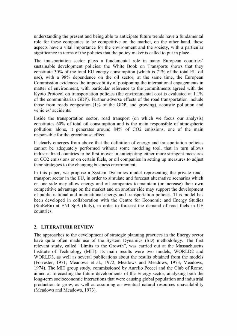
The transportation sector plays a fundamental role in many European countries’
sustainable development policies: the White Book on Transports shows that they
constitute 30% of the total EU energy consumption (which is 71% of the total EU oil
use), with a 98% dependence on the oil sector; at the same time, the European
Commission evidences the impossibility of postponing the international engagements in
matter of environment, with particular reference to the commitments agreed with the
Kyoto Protocol on transportation policies (the environmental cost is evaluated at 1.1%
of the communitarian GDP). Further adverse effects of the road transportation include
those from roads congestion (1% of the GDP, and growing), acoustic pollution and
vehicles’ accidents.
Inside the transportation sector, road transport (on which we focus our analysis)
constitutes 60% of total oil consumption and is the main responsible of atmospheric
pollution: alone, it generates around 84% of CO2 emissions, one of the main
responsible for the greenhouse effect.
It clearly emerges from above that the definition of energy and transportation policies
cannot be adequately performed without some modeling tool, that in turn allows
industrialized countries to be first mover in anticipating either more stringent measures
on CO2 emissions or on certain fuels, or oil companies in setting up measures to adjust
their strategies to the changing business environment.
In this paper, we propose a System Dynamics model representing the private road-
transport sector in the EU, in order to simulate and forecast alternative scenarios which
on one side may allow energy and oil companies to maintain (or increase) their own
competitive advantage on the market and on another side may support the development
of public national and international energy and transportation policies. This model has
been developed in collaboration with the Centre for Economic and Energy Studies
(StuEcEn) at ENI SpA (Italy), in order to forecast the demand of road fuels in UE
countries.
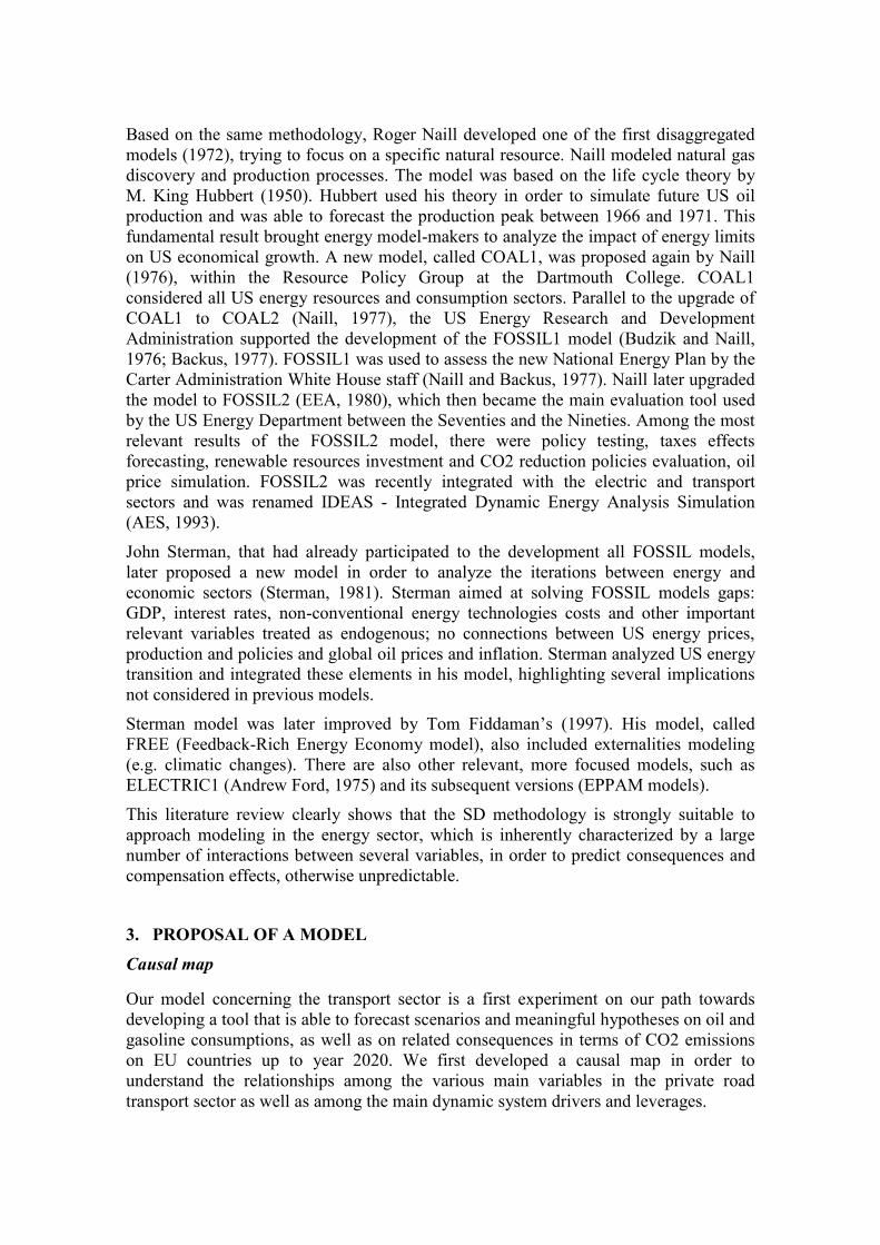
2. LITERATURE REVIEW
The approaches to the development of strategic planning practices in the Energy sector
have quite often made use of the System Dynamics (SD) methodology. The first
relevant study, called “Limits to the Growth”, was carried out at the Massachusetts
Institute of Technology (MIT): its main results were two models, WORLD2 and
WORLD3, as well as several publications about the results obtained from the models
(Forrester, 1971; Meadows et al., 1972; Meadows and Meadows, 1973, Meadows,
1974). The MIT group study, commissioned by Aurelio Peccei and the Club of Rome,
aimed at forecasting the future developments of the Energy sector, analyzing both the
long-term socioeconomic interactions that were causing global population and industrial
production to grow, as well as assuming an eventual natural resources unavailability
(Meadows and Meadows, 1973).
Based on the same methodology, Roger Naill developed one of the first disaggregated
models (1972), trying to focus on a specific natural resource. Naill modeled natural gas
discovery and production processes. The model was based on the life cycle theory by
M. King Hubbert (1950). Hubbert used his theory in order to simulate future US oil
production and was able to forecast the production peak between 1966 and 1971. This
fundamental result brought energy model-makers to analyze the impact of energy limits
on US economical growth. A new model, called COAL1, was proposed again by Naill
(1976), within the Resource Policy Group at the Dartmouth College. COAL1
considered all US energy resources and consumption sectors. Parallel to the upgrade of
COAL1 to COAL2 (Naill, 1977), the US Energy Research and Development
Administration supported the development of the FOSSIL1 model (Budzik and Naill,
1976; Backus, 1977). FOSSIL1 was used to assess the new National Energy Plan by the
Carter Administration White House staff (Naill and Backus, 1977). Naill later upgraded
the model to FOSSIL2 (EEA, 1980), which then became the main evaluation tool used
by the US Energy Department between the Seventies and the Nineties. Among the most
relevant results of the FOSSIL2 model, there were policy testing, taxes effects
forecasting, renewable resources investment and CO2 reduction policies evaluation, oil
price simulation. FOSSIL2 was recently integrated with the electric and transport
sectors and was renamed IDEAS - Integrated Dynamic Energy Analysis Simulation
(AES, 1993).
John Sterman, that had already participated to the development all FOSSIL models,
later proposed a new model in order to analyze the iterations between energy and
economic sectors (Sterman, 1981). Sterman aimed at solving FOSSIL models gaps:
GDP, interest rates, non-conventional energy technologies costs and other important
relevant variables treated as endogenous; no connections between US energy prices,
production and policies and global oil prices and inflation. Sterman analyzed US energy
transition and integrated these elements in his model, highlighting several implications
not considered in previous models.
Sterman model was later improved by Tom Fiddaman’s (1997). His model, called
FREE (Feedback-Rich Energy Economy model), also included externalities modeling
(e.g. climatic changes). There are also other relevant, more focused models, such as
ELECTRIC1 (Andrew Ford, 1975) and its subsequent versions (EPPAM models).
This literature review clearly shows that the SD methodology is strongly suitable to
approach modeling in the energy sector, which is inherently characterized by a large
number of interactions between several variables, in order to predict consequences and
compensation effects, otherwise unpredictable.
3. PROPOSAL OF A MODEL
Causal map
Our model concerning the transport sector is a first experiment on our path towards
developing a tool that is able to forecast scenarios and meaningful hypotheses on oil and
gasoline consumptions, as well as on related consequences in terms of CO2 emissions
on EU countries up to year 2020. We first developed a causal map in order to
understand the relationships among the various main variables in the private road
transport sector as well as among the main dynamic system drivers and leverages.

The main driver on fuel consumption is represented by the transportation demand in
terms of passengers per kilometer in each year. The strong link between the GDP and
the general level of transportations, poses an important question concerning the growth
of the transportation demand. As it emerges by looking at the literature, many economic
studies, while focusing on this relationship, have hypothesized a growth of demand as
strictly in line with the growth of the GDP, but did not factor in many other aspects that,
as a matter of fact, determine a stabilization in the system due to physical and structural
constraints. Such constraints would thus necessarily bring to a saturation in transport
demand while the GDP can keep on growing.
Such a relationship is obviously also influenced by the characteristics of the
geographical area which is the focus of our analysis. Rapid developing and emerging
countries in the middle of their industrial, economic as well as also demographic
development, are about to reach the pro-capita annual revenue levels (about 5000$/year)
beyond which, historically, it is possible to note a great increase in car use and thus an
acceleration in oil products demand for transportation. In the same way, many countries
in Eastern Europe are having an important economic growth, which thus influences the
transportation demand.
As previously mentioned, efficiency must be considered as the key element in fuels and
oil consumption. EU has an overall vehicle fleet average efficiency that is far higher
than USA’s one. This depends of course on the average vehicle’s construction
characteristics as well as on various factors that, as a matter of fact, have determined
market dynamics over the years. Among the most relevant aspects, we cannot neglect
the fuel price, which has historically been much cheaper than in Europe, thus allowing
citizens to choose larger and more powerful cars (i.e.: SUVs), which generally have an
higher fuel consumption. The graph below (Figure 1) relates the average efficiency of
EU to US fleets from 1985 to 2007.
Figure 1: Comparison of US and EU average fleets efficiency
0.000
0.200
0.400
0.600
0.800
1.000
1.200
1.400
19
78
19
79
19
80
19
81
19
82
19
83
19
84
19
85
19
86
19
87
19
88
19
89
19
90
19
91
19
92
19
93
19
94
19
95
19
96
19
97
19
98
19
99
20
00
20
01
20
02
20
03
20
04
20
05
20
06
20
07
eu
ro/lit
er
0
2
4
6
8
10
12
14
16
km
/lit
er
Automotive Diesel Big 5 UE Premium Unleaded 95 RON big 5 UE
Premium Unleaded 95 RON US Average EU15 car specific consumption (right axis)
Average U.S. light duty fuel efficiency (right axis)
As we can see from the data behaviour, vehicles’ efficiency has played a fundamental
role: the UE trend underlines an improvement in efficiency due to lower costs sustained
to satisfy the yearly transportation demand of passengers. As an example, it is today
well known how, over the last decade, diesel engines have reached a great percentage in
new vehicles’ registrations, due to their better efficiency and thus by the straightforward
lower consumption.
Such a market tendency is quite important and has to be carefully accounted for by the
great oil companies in order to sketch out a possible trend from today until the next
decades. The demand for fuel may in fact bring, on a short to medium term, to an
increase in diesel demand and a relative decrease in gasoline use. However, other
various aspects have to be accounted for: at the moment, diesel vehicles’ penetration
rates are quite different in each EU country, just like the pro-capita welfare level. Also,
it must be accounted for the possibility of a surge and diffusion of new alternative
engine technologies (hybrid or fully electrical vehicles), of small and light cars, thus
having more efficient engines, of different fuel price dynamics and relative taxations,
which may balance back the growing trend in diesel use.
Another important issue influencing fuel use is the average distance travelled per
vehicle (measured in kilometres per year): also in this case, we can notice a gap between
the US and EU given by the substantial differences that arise from the different
contexts, from the average inhabitants density (higher in the EU) and from the fuel
prices (lower in the US). The decrease of petrol use in the US from its peak in 2005,
later also amplified by the economic crisis, is partly explained by the higher prices to
the final consumer at the gas stations during the last years.

Figure 2: Overall causal map
So, given the overall causal map in Figure 2, which depicts the situations explained
above, we can identify four different feedback loops, three of which are evidenced in
figure 3 and the fourth, a reinforcing one, is identified by the external path to our map.
When we later got to the quantitative modelling phase, by neglecting the road
congestion effects on the average vehicles’ efficiency, we evidenced the presence of
only two feedback loops with different polarity, whose interaction determined a “limits
to the growth” archetype.
road network
traffic
congestion
average on road
fuel efficiency
average kilometric
cost per vehicle
incentive scheme for
buying new cars
new cars price
indexnew cars
population
total private travel
demand
total vehicle fleet
+
total vehicle
kilometers travelled+
+
+
-
-
-
average age of
cars
-
gdp per-capita
average number of
persons in a vehicle
environmental
policies-
distance travel per
vehicle
+
fuel
consumption
CO2 emission
+
+
-cars scrappage
Brent price
fuel price+
+
+
distance travel
per-capita
+
+
-
+
-
-
-
+
+
-
kilometric cost
per-capita-
-
gdp-
+
+
+
-
+
fuel taxes +

Figure 3: Feedback loops
Reading the causal loop diagram in Figure 3 is quite simple: as the “total private travel
demand” grows, the “total vehicle kilometres travelled” grows too, thus increasing the
“distance travelled per vehicle”, which in turn positively affects the “traffic congestion”
factor. The latter, negatively influences the “average on road fuel efficiency”, whose
eventual improvement may bring to a decrease in the “average kilometric cost per
vehicle” and consequently the “kilometric cost per-capita”. The latter, in turn negatively
influences the “ distance travelled per-capita”, whose eventual increase may lead back
to an increase in the “total private travel demand ”, thus closing this balancing loop.
However, the quantitative modelling phase usually further clears the overall picture
concerning the existing relationships among the various parts of the system, eventually
requesting to go back to the qualitative phase if some new considerations arise after the
first simulation runs. This situation is particularly evident with reference to exogenous
variables: the unavailability of fundamental data may even imply bringing deep
modifications to the causal map itself, and thus the relationships among the variables of
the system, thus evidencing sometimes also different dynamic structures.
As an example, with reference to the causal loop depicted in Figure 3, the “road
congestion” variable represents a very important factor into that loop since it generates
dynamics related to its behaviour over time. We can thus suppose that such a factor may
be described by a mathematical function. In the reality, the road congestion concept
sums up a whole bunch of articulated considerations that may not be summarized by
just a mathematical or analytic expression; rather, it alone might be described by
another model, thus including other variables, levels, flows, etc.
This issue is quite important since it helps understand how the maybe excessive but
necessary simplification in the definition of some elements may generate dynamical
behaviours responsible for undesired distortions, independently of the conceived model
and its goal. For this reason, we decided to focus our attention on how to represent a
substitute element rather than inserting a simplified one, which may generate too much
total private travel
demand
distance travel per
vehicle
average kilometric
cost per vehicle
total vehicle
kilometers travelled
kilometric cost
per-capita
distance travel
per-capita +
average number of
persons in a vehicle
+
-
-
R1
traffic
congestion
average on road
fuel efficiency
+
-
-
B2
B1
-
+
+-
R2

evident mistakes in describing the system’s behaviour. We decided to represent the
“road congestion” as a qualitative indicator (condensed in a slight decrease of fuel
efficiency related to congestion increase) rather than a quantitative one.
Stock & Flow Model
Fuels Prices
The following Figure 4 shows a sub-model describing how the fuel-pump prices are
determined (the LPG is not considered anymore in this part of the model), starting from
the Brent price and, step by step, translating it into a final pump price for diesel and
gasoline (in Euro).
Figure 4: Final fuel price model
A time series on the quarterly Brent price (in dollars), from January 1995 to January
2031 is included in the model by uploading an excel file containing the estimates
provided by the “StuEcEn” Center of Economic and Energy Studies and updated in
coherence with the latest official scenario. We won’t delve into this variable’s
estimation process, even though, nowadays, it constitutes one of the most interesting
aspects on international markets. Moreover, the complexity of such a system requires a
dedicated model, besides the global evolution of energy, political-economic and social
considerations.
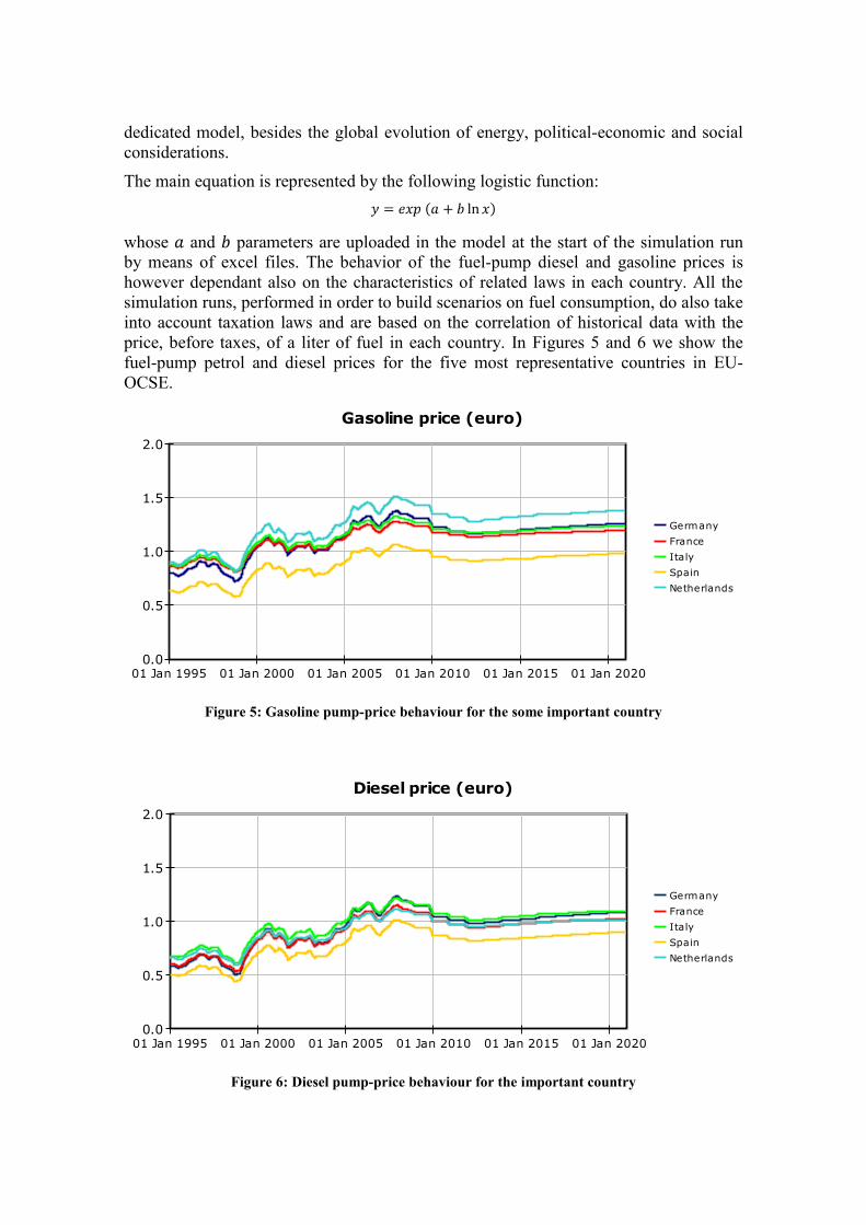
The main equation is represented by the following logistic function:
whose and parameters are uploaded in the model at the start of the simulation run
by means of excel files. The behavior of the fuel-pump diesel and gasoline prices is
however dependant also on the characteristics of related laws in each country. All the
simulation runs, performed in order to build scenarios on fuel consumption, do also take
into account taxation laws and are based on the correlation of historical data with the
price, before taxes, of a liter of fuel in each country. In Figures 5 and 6 we show the
fuel-pump petrol and diesel prices for the five most representative countries in EU-
OCSE.
Figure 5: Gasoline pump-price behaviour for the some important country
Figure 6: Diesel pump-price behaviour for the important country
Gasoline price (euro)
01 Jan 1995 01 Jan 2000 01 Jan 2005 01 Jan 2010 01 Jan 2015 01 Jan 20200.0
0.5
1.0
1.5
2.0
Germany
France
Italy
Spain
Netherlands
Diesel price (euro)
01 Jan 1995 01 Jan 2000 01 Jan 2005 01 Jan 2010 01 Jan 2015 01 Jan 20200.0
0.5
1.0
1.5
2.0
Germany
France
Italy
Spain
Netherlands
Technology-improvement Scenario
This scenario takes into account also the market potential of hybrid engine and electric
vehicles, as well as of fossil gaseous fuels (LPG, CNG) on a medium-to-long term
basis. The competitiveness of electric vehicles compared to traditional internal
combustion engines is likely to depend in the future on the cost and autonomy of battery
packs, as well as on the availability of some metals used in building electric engines and
battery packs themselves, as also on the price of electricity. Such uncertainties make it
particularly difficult to choose among the exogenous variables to include in the model.
Vehicle fleet’s dynamics
The level concerning the total amount of vehicles (or Total Fleet) is a time dependant
matrix based on three components: age class of the fleet, country, fuel type. Thanks to a
sufficiently detailed database, it was possible to initialize this level with the starting date
of our simulation runs. It was thus possible to obtain a detailed description of the fleet
development behaviour. It is interesting to point out that cars are not simply treated as
belonging to a same class, rather they are subdivided according to 25 classes of age, the
last of which identifies cars with more than 24 years. Thus the model accounts for the
obviously different average efficiency and consumption that each class displays.
The flows affecting such a state of the system do always refer to car scrappings and
exports (outflows) and new cars registrations (inflow).
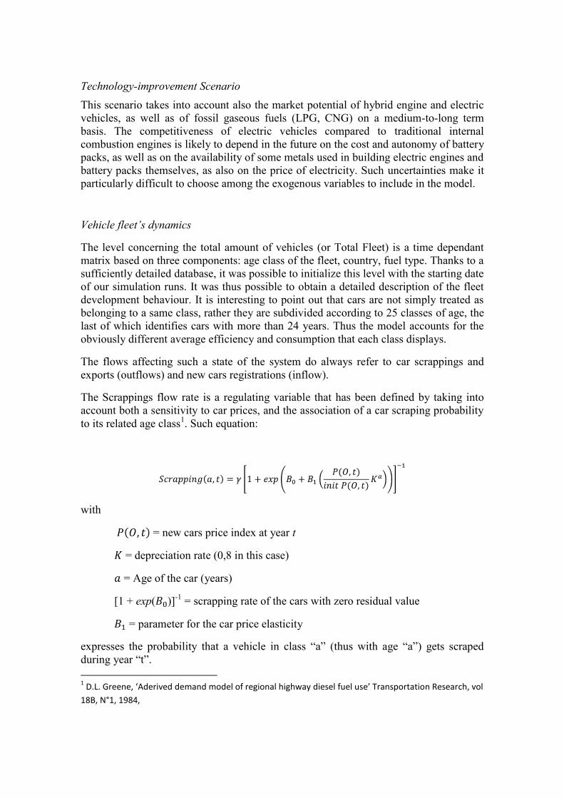
The Scrappings flow rate is a regulating variable that has been defined by taking into
account both a sensitivity to car prices, and the association of a car scraping probability
to its related age class1. Such equation:
with
= new cars price index at year t
= depreciation rate (0,8 in this case)
= Age of the car (years)
[1 + exp( )]-1
= scrapping rate of the cars with zero residual value
= parameter for the car price elasticity
expresses the probability that a vehicle in class “a” (thus with age “a”) gets scraped
during year “t”.
1 D.L. Greene, ‘Aderived demand model of regional highway diesel fuel use’ Transportation Research, vol
18B, N°1, 1984,
As long as vehicles’ aging is concerned, we modeled an aging chain by considering a
yearly shift of all vehicles belonging to a certain age class to the next one. As long as
the inflow rate to the aging chain is concerned, while
car registrations historical data2 is derived during the simulation thanks to an excel file
imported in the initialization phase, at the start of year 2005 we have set two
stocks&flows sub-models so to regulate such an inflow variable as a logistic-growth
curve (S-shaped), thus depicting the behavior in each EU country of newly registered
vehicles (first submodel) as well as the ratio of the rate of penetration of diesel-engine
vehicles to the amount of vehicles in the overall fleet (second submodel).
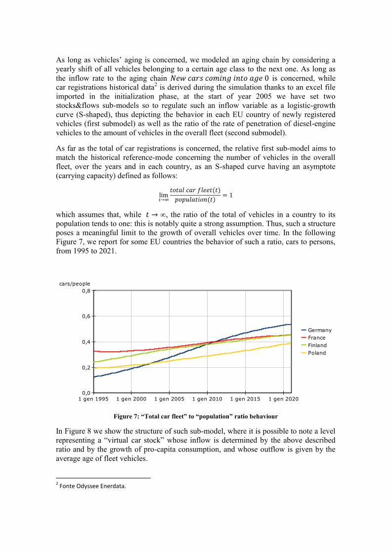
As far as the total of car registrations is concerned, the relative first sub-model aims to
match the historical reference-mode concerning the number of vehicles in the overall
fleet, over the years and in each country, as an S-shaped curve having an asymptote
(carrying capacity) defined as follows:
which assumes that, while , the ratio of the total of vehicles in a country to its
population tends to one: this is notably quite a strong assumption. Thus, such a structure
poses a meaningful limit to the growth of overall vehicles over time. In the following
Figure 7, we report for some EU countries the behavior of such a ratio, cars to persons,
from 1995 to 2021.
Figure 7: “Total car fleet” to “population” ratio behaviour
In Figure 8 we show the structure of such sub-model, where it is possible to note a level
representing a “virtual car stock” whose inflow is determined by the above described
ratio and by the growth of pro-capita consumption, and whose outflow is given by the
average age of fleet vehicles.
2 Fonte Odyssee Enerdata.
1 gen 1995 1 gen 2000 1 gen 2005 1 gen 2010 1 gen 2015 1 gen 20200,0
0,2
0,4
0,6
0,8
cars/people
Germany
France
Finland
Poland
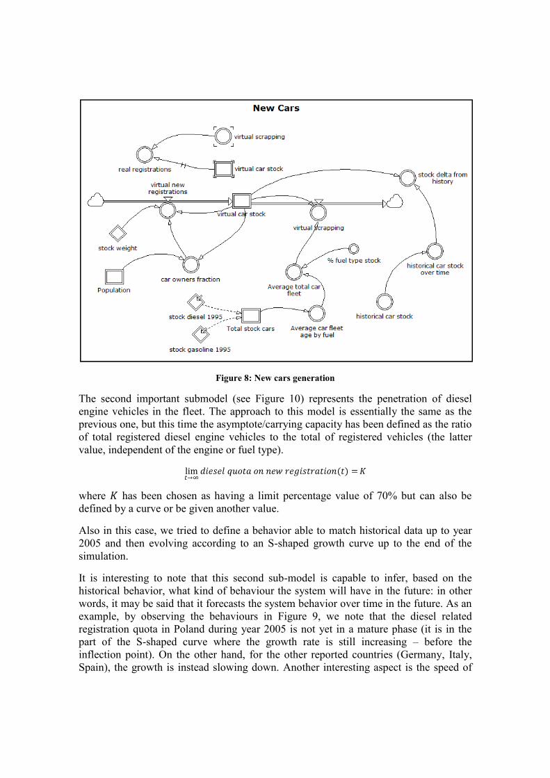
Figure 8: New cars generation
The second important submodel (see Figure 10) represents the penetration of diesel
engine vehicles in the fleet. The approach to this model is essentially the same as the
previous one, but this time the asymptote/carrying capacity has been defined as the ratio
of total registered diesel engine vehicles to the total of registered vehicles (the latter
value, independent of the engine or fuel type).
where has been chosen as having a limit percentage value of 70% but can also be
defined by a curve or be given another value.
Also in this case, we tried to define a behavior able to match historical data up to year
2005 and then evolving according to an S-shaped growth curve up to the end of the
simulation.
It is interesting to note that this second sub-model is capable to infer, based on the
historical behavior, what kind of behaviour the system will have in the future: in other
words, it may be said that it forecasts the system behavior over time in the future. As an
example, by observing the behaviours in Figure 9, we note that the diesel related
registration quota in Poland during year 2005 is not yet in a mature phase (it is in the
part of the S-shaped curve where the growth rate is still increasing – before the
inflection point). On the other hand, for the other reported countries (Germany, Italy,
Spain), the growth is instead slowing down. Another interesting aspect is the speed of
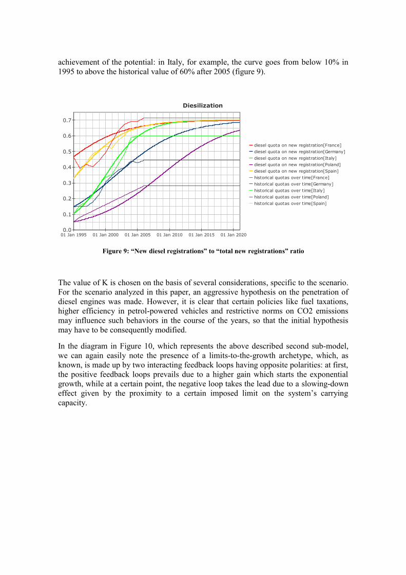
achievement of the potential: in Italy, for example, the curve goes from below 10% in
1995 to above the historical value of 60% after 2005 (figure 9).
Figure 9: “New diesel registrations” to “total new registrations” ratio
The value of K is chosen on the basis of several considerations, specific to the scenario.
For the scenario analyzed in this paper, an aggressive hypothesis on the penetration of
diesel engines was made. However, it is clear that certain policies like fuel taxations,
higher efficiency in petrol-powered vehicles and restrictive norms on CO2 emissions
may influence such behaviors in the course of the years, so that the initial hypothesis
may have to be consequently modified.
In the diagram in Figure 10, which represents the above described second sub-model,
we can again easily note the presence of a limits-to-the-growth archetype, which, as
known, is made up by two interacting feedback loops having opposite polarities: at first,
the positive feedback loops prevails due to a higher gain which starts the exponential
growth, while at a certain point, the negative loop takes the lead due to a slowing-down
effect given by the proximity to a certain imposed limit on the system’s carrying
capacity.
Diesilization
01 Jan 1995 01 Jan 2000 01 Jan 2005 01 Jan 2010 01 Jan 2015 01 Jan 20200.0
0.1
0.2
0.3
0.4
0.5
0.6
0.7
diesel quota on new registration[France]
diesel quota on new registration[Germany]
diesel quota on new registration[Italy]
diesel quota on new registration[Poland]
diesel quota on new registration[Spain]
historical quotas over time[France]
historical quotas over time[Germany]
historical quotas over time[Italy]
historical quotas over time[Poland]
historical quotas over time[Spain]
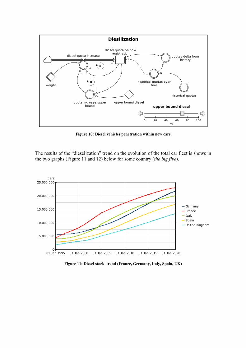
Figure 10: Diesel vehicles penetration within new cars
The results of the “dieselization” trend on the evolution of the total car fleet is shows in
the two graphs (Figure 11 and 12) below for some country (the big five).
Figure 11: Diesel stock trend (France, Germany, Italy, Spain, UK)
Diesilization
upper bound diesel
0 20 40 60 80 100
%
B
R
+
+
+
-
diesel quota on newregistration
diesel quota increase
quota increase upperbound
historical quotas
quotas delta fromhistory
weighthistorical quotas over
time
upper bound diesel
Stock diesel : Francia, Germania, Italia, Spagna, Uk
01 Jan 1995 01 Jan 2000 01 Jan 2005 01 Jan 2010 01 Jan 2015 01 Jan 20200
5,000,000
10,000,000
15,000,000
20,000,000
25,000,000
cars
Germany
France
Italy
Spain
United Kingdom
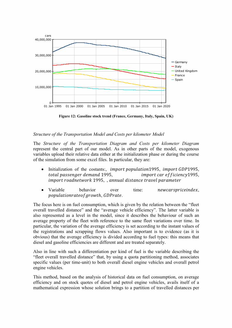
Figure 12: Gasoline stock trend (France, Germany, Italy, Spain, UK)
Structure of the Transportation Model and Costs per kilometer Model
The Structure of the Transportation Diagram and Costs per kilometer Diagram
represent the central part of our model. As in other parts of the model, exogenous
variables upload their relative data either at the initialization phase or during the course
of the simulation from some excel files. In particular, they are:
Initialization of the costants:, , ,
, ,
, ,
Variable behavior over time: ,
, .
The focus here is on fuel consumption, which is given by the relation between the “fleet
overall travelled distance” and the “average vehicle efficiency”. The latter variable is
also represented as a level in the model, since it describes the behaviour of such an
average property of the fleet with reference to the same fleet variations over time. In
particular, the variation of the average efficiency is set according to the instant values of
the registrations and scrapping flows values. Also important is to evidence (as it is
obvious) that the average efficiency is divided according to fuel types: this means that
diesel and gasoline efficiencies are different and are treated separately.
Also in line with such a differentiation per kind of fuel is the variable describing the
“fleet overall travelled distance” that, by using a quota partitioning method, associates
specific values (per time-unit) to both overall diesel engine vehicles and overall petrol
engine vehicles.
This method, based on the analysis of historical data on fuel consumption, on average
efficiency and on stock quotes of diesel and petrol engine vehicles, avails itself of a
mathematical expression whose solution brings to a partition of travelled distances per
Stock gasoline : Francia, Germania, Italia, Spagna, Uk
01 Jan 1995 01 Jan 2000 01 Jan 2005 01 Jan 2010 01 Jan 2015 01 Jan 20200
10,000,000
20,000,000
30,000,000
40,000,000
cars
Germany
Italy
United Kingdom
France
Spain

vehicle-power type. Thus, a specific variable “distance travelled quotas per fuel”
determines a variable partition percentage which is also function of the evolutions in the
overall fleet.
From a structural point of view, a fundamental element has to be recognized in the
dynamics of the “car transportation demand”. Its variation has been defined as a
function of the “pro-capita car transportation demand” and “population”. The former is
related by a logistic function to the behaviour of the “private pro-capita consumption”
and of the “pro-capita cost per kilometer”. This way it was possible to represent both an
income and a transportation cost elasticity, by means of a specific variable defined as
follows:
This variable will serve the purpose to dampen the growth of each country’s “pro-capita
car transportation demand”, thus as a matter of fact constraining it, on average terms, to
the welfare growth. In order to monitor and contain the behaviour of the “transportation
demand”, we developed a control panel through which it is possible to fix a maximum
limit to the development of “pro-capita car transportation demand”. Such a panel leans
on an underlying submodel which presents again the recurring archetypical structure of
the limits to the growth, so to take into account both the development of public
transportation policies rather than other policies aiming at reducing the “private per-
capita travelled distance” (i.e.: by means of urban planning, congestion charge, etc.).
The following Figure 13 shows this sub-model.
Figure 13: Per-capita car transportation demand limits
A switch panel allows choosing, during each simulation run, whether to intervene on
demand by limiting it (according to slider controls which are not shown in the figure) or
to leave it in a free evolution according to the equations ruling its dynamics.
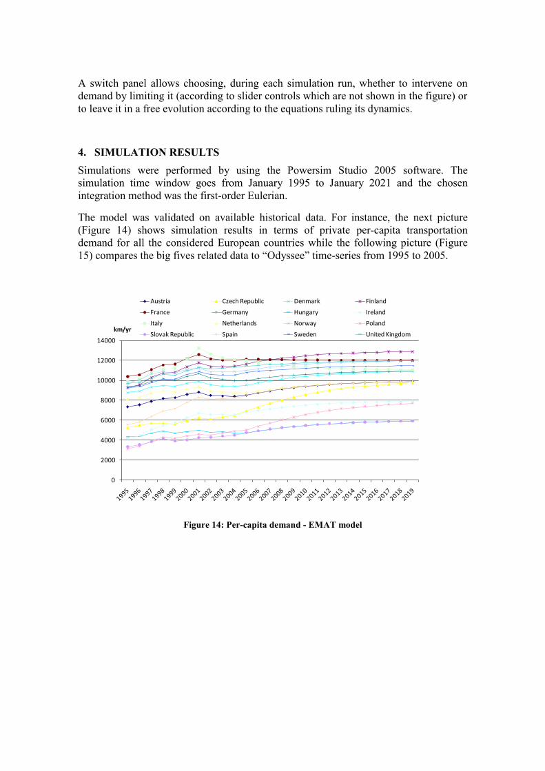
4. SIMULATION RESULTS
Simulations were performed by using the Powersim Studio 2005 software. The
simulation time window goes from January 1995 to January 2021 and the chosen
integration method was the first-order Eulerian.
The model was validated on available historical data. For instance, the next picture
(Figure 14) shows simulation results in terms of private per-capita transportation
demand for all the considered European countries while the following picture (Figure
15) compares the big fives related data to “Odyssee” time-series from 1995 to 2005.
Figure 14: Per-capita demand - EMAT model
0
2000
4000
6000
8000
10000
12000
14000
Austria Czech Republic Denmark Finland
France Germany Hungary Ireland
Italy Netherlands Norway Poland
Slovak Republic Spain Sweden United Kingdomkm/yr
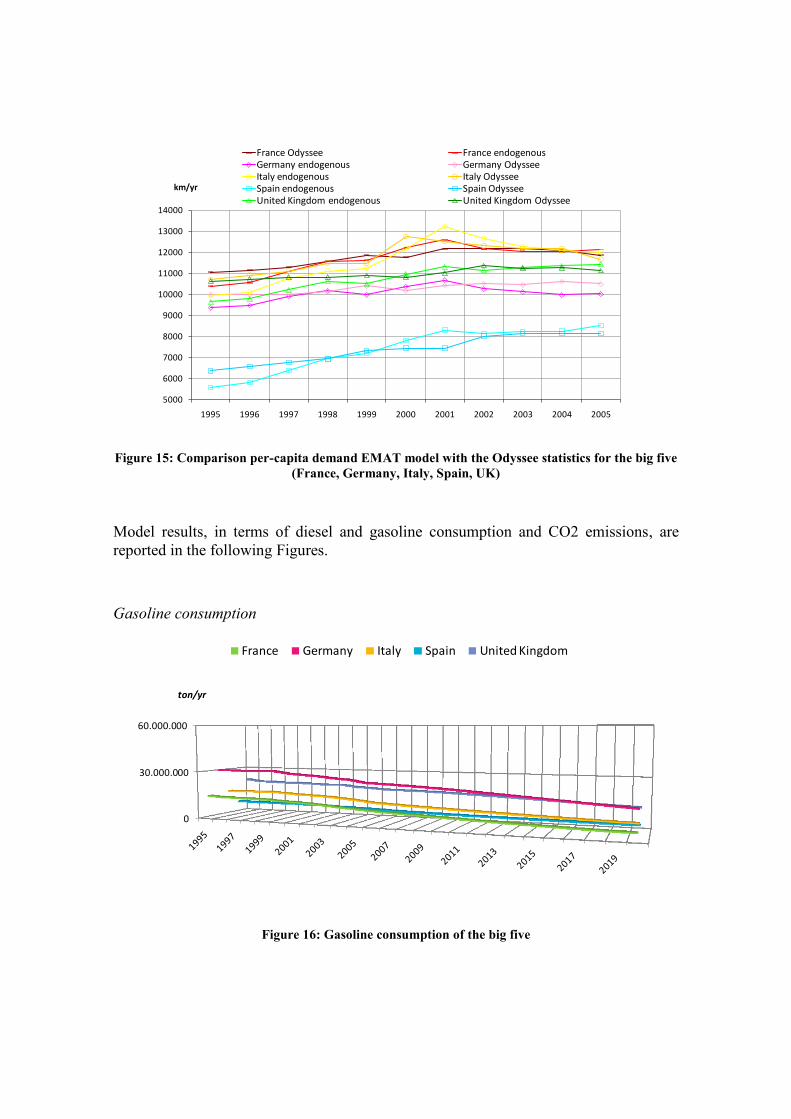
Figure 15: Comparison per-capita demand EMAT model with the Odyssee statistics for the big five
(France, Germany, Italy, Spain, UK)
Model results, in terms of diesel and gasoline consumption and CO2 emissions, are
reported in the following Figures.
Gasoline consumption
Figure 16: Gasoline consumption of the big five
5000
6000
7000
8000
9000
10000
11000
12000
13000
14000
1995 1996 1997 1998 1999 2000 2001 2002 2003 2004 2005
France Odyssee France endogenousGermany endogenous Germany OdysseeItaly endogenous Italy OdysseeSpain endogenous Spain OdysseeUnited Kingdom endogenous United Kingdom Odyssee
km/yr
0
30.000.000
60.000.000
France Germany Italy Spain United Kingdom
ton/yr
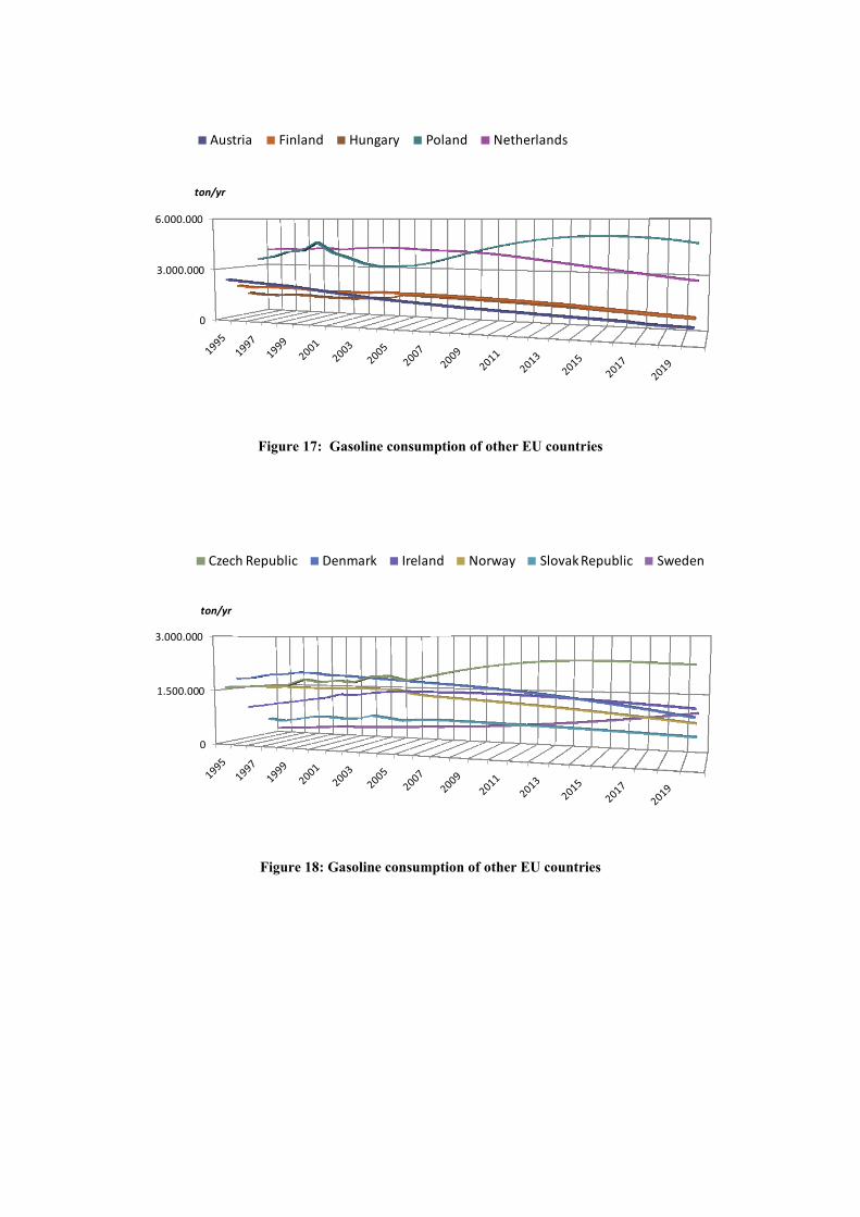
Figure 17: Gasoline consumption of other EU countries
Figure 18: Gasoline consumption of other EU countries
0
3.000.000
6.000.000
Austria Finland Hungary Poland Netherlands
ton/yr
0
1.500.000
3.000.000
Czech Republic Denmark Ireland Norway Slovak Republic Sweden
ton/yr
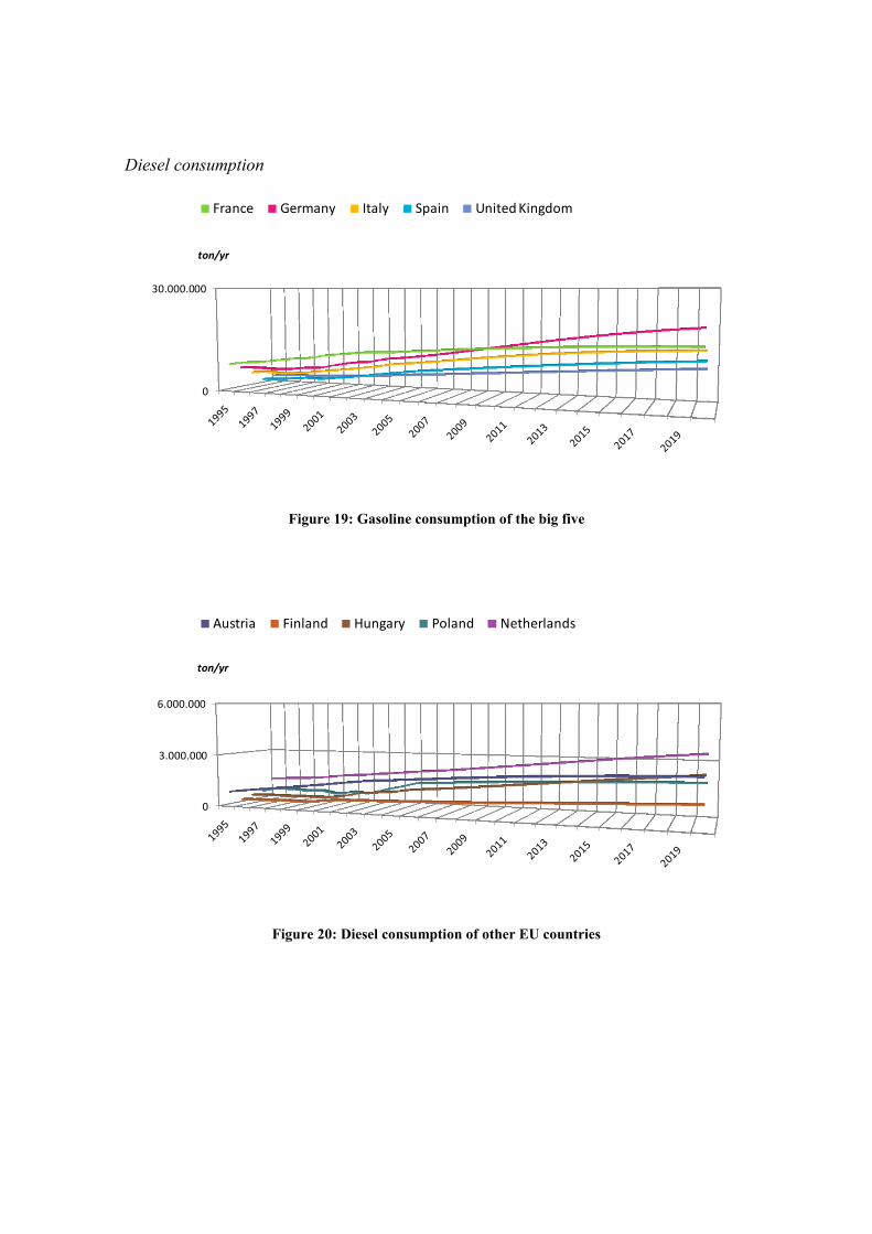
Diesel consumption
Figure 19: Gasoline consumption of the big five
Figure 20: Diesel consumption of other EU countries
0
30.000.000
France Germany Italy Spain United Kingdom
ton/yr
0
3.000.000
6.000.000
Austria Finland Hungary Poland Netherlands
ton/yr
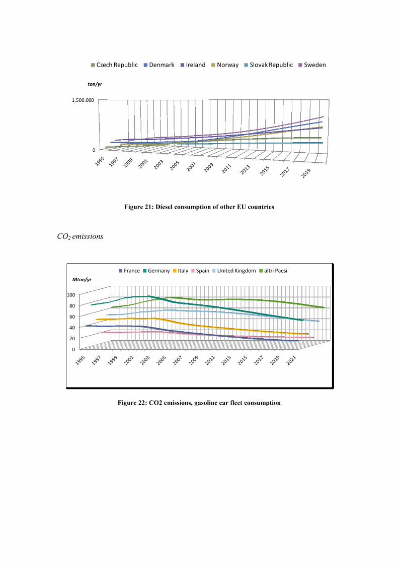
Figure 21: Diesel consumption of other EU countries
CO2 emissions
Figure 22: CO2 emissions, gasoline car fleet consumption
0
1.500.000
Czech Republic Denmark Ireland Norway Slovak Republic Sweden
ton/yr
0
20
40
60
80
100
France Germany Italy Spain United Kingdom altri Paesi
Mton/yr
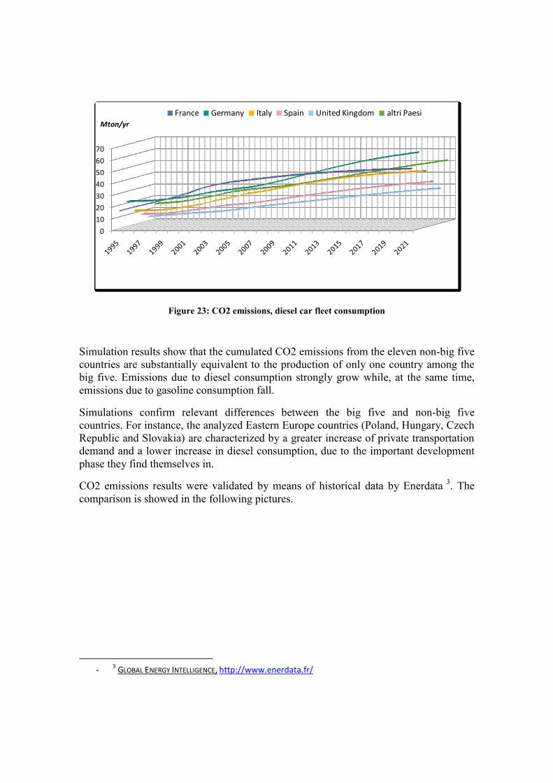
Figure 23: CO2 emissions, diesel car fleet consumption
Simulation results show that the cumulated CO2 emissions from the eleven non-big five
countries are substantially equivalent to the production of only one country among the
big five. Emissions due to diesel consumption strongly grow while, at the same time,
emissions due to gasoline consumption fall.
Simulations confirm relevant differences between the big five and non-big five
countries. For instance, the analyzed Eastern Europe countries (Poland, Hungary, Czech
Republic and Slovakia) are characterized by a greater increase of private transportation
demand and a lower increase in diesel consumption, due to the important development
phase they find themselves in.
CO2 emissions results were validated by means of historical data by Enerdata 3
. The
comparison is showed in the following pictures.
-
3 GLOBAL ENERGY INTELLIGENCE, http://www.enerdata.fr/
0
10
20
30
40
50
60
70
France Germany Italy Spain United Kingdom altri PaesiMton/yr
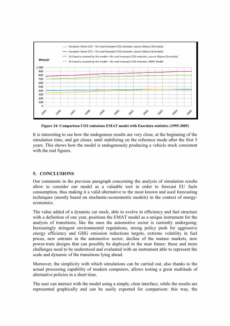
Figure 24: Comparison CO2 emissions EMAT model with Enerdata statistics (1995-2005)
It is interesting to see how the endogenous results are very close, at the beginning of the
simulation time, and get closer, until stabilizing on the reference mode after the first 5
years. This shows how the model is endogenously producing a vehicle stock consistent
with the real figures.
5. CONCLUSIONS
Our comments in the previous paragraph concerning the analysis of simulation results
allow to consider our model as a valuable tool in order to forecast EU fuels
consumption, thus making it a valid alternative to the most known and used forecasting
techniques (mostly based on stochastic-econometric models) in the context of energy-
economics.
The value added of a dynamic car stock, able to evolve in efficiency and fuel structure
with a definition of one year, positions the EMAT model as a unique instrument for the
analysis of transitions, like the ones the automotive sector is currently undergoing.
Increasingly stringent environmental regulations, strong policy push for aggressive
energy efficiency and GHG emission reductions targets, extreme volatility in fuel
prices, new entrants in the automotive sector, decline of the mature markets, new
power-train designs that can possibly be deployed in the near future: these and more
challenges need to be understood and evaluated with an instrument able to represent the
scale and dynamic of the transitions lying ahead.
Moreover, the simplicity with which simulations can be carried out, also thanks to the
actual processing capability of modern computers, allows testing a great multitude of
alternative policies in a short time.
The user can interact with the model using a simple, clear interface, while the results are
represented graphically and can be easily exported for comparison: this way, the
relevance and impact of different policies can be compared. Moreover, unlike most of
the classical spreadsheet or econometric models, the synergies among different policies
are accounted by the feedback structure of the model, making possible the evaluation of
sets of policies (i.e. subsidies, standards, different biofuels mandates, etc.) rather than
evaluating only one at a time.
EMAT is the demonstration of how system dynamics models can make a difference
when the object of the analysis is a sector that is undergoing major transitions and
different challenges. The comparison with the results from well-established
econometrical models shows how the system dynamics methodology has a competitive
advantage in describing a world where nothing is linear and feedbacks are at work.
EMAT is able to provide insights on the scale of the threats oil companies and car
manufacturers are facing today. At the same time, it can guide policy makers in the
difficult task of coping with global challenges, using an advanced and yet simple tool to
prevent the arising of unintended consequences from the interactions of the many
different policies they are called to put in place.
6. REFERENCES
Alternative Energy Systems, (1993) An Overview of the IDEAS Model: A Dynamic
Long-Term Policy Simulation of U.S. Energy Supply and Demand. AES Corporation.
1001 North 19th Street. Arlington, VA.
Backus, G. A., (1977) FOSSIL1: Documentation. DSD #86. Resource Policy Center.
Dartmouth College, Hanover, New Hampshire.
Budzik P. M., Naill R. F., (1976) FOSSIL1: A policy analysis model of the U.S. energy
transition, Source Winter Simulation Conference archive - Proceedings of the 76
Bicentennial conference on Winter simulation table of contents, Gaithersburg, MD, pp.
145 - 152 .
Energy and Environmental Analysis, Inc., (1980) FOSSIL2: Energy Policy Model
Documentation, Department of Energy Contract No. AC01-79PE70143, Assistant
Secretary for Policy, Planning and Analysis. Washington, D.C.
Fiddaman, T. S., (1997) Feedback Complexity in Integrated Climate-Economy Models.
Doctoral Thesis Submitted to the Alfred P. Sloan School of Management.
Massachusetts Institute of Technology. Cambridge, MA.
Ford, A., (1975) A Dynamic Model of the U.S. Electric Utility Industry. Doctoral Thesis
Submitted to the Thayer School of Engineering. DSD #28, 31. Dartmouth College.
Hanover, New Hampshire.
Forrester, J. W., (1971) World Dynamics, Productivity Press Inc.
Hubbert, M.K., (1950) Energy from fossil fuels, Annual Report of the Smithsonian
Institution, June 30, pp. 255-271.
Meadows D.H., Meadows D.L., Randers J., Behrens III W.W., (1972) The Limits to
Growth. Washington, D.C.: Potomac Associates, New American Library.
Meadows D.L., Meadows, D.H., (1973) Toward Global Equilibrium: Collected Papers,
Productivity Press Inc.
Meadows D.L., (1974) Dynamics of Growth in a Finite World, Productivity Press Inc.
Naill, R.F., (1972) Managing the Discovery Life Cycle of a Finite Resource: A Case
Study of U.S. Natural Gas. Master's Thesis Submitted to the Alfred P. Sloan School of
Management. Massachusetts Institute of Technology. Cambridge, MA
Naill, R. F., (1976) COAL1: A Dynamic Model for the Analysis of United States Energy
Policy. Doctoral Thesis Submitted to the Thayer School of Engineering. DSD #54.
Dartmouth College. Hanover, New Hampshire
Naill, R. F., (1977) Managing the energy transition: a system dynamics search for
alternatives to oil and gas, Ballinger Publishing Company, Cambridge, MA.

Naill, R.F. ; Backus, G.A., (1977) Evaluating the national energy plan, Technol. Rev.,
vol. 79:8, Dartmouth Coll., Hanover, NH
Sterman, J. D., (1981) The Energy Transition and the Economy: A System Dynamics
Approach. Doctoral Thesis Submitted to the Alfred P. Sloan School of Management.
Massachusetts Institute of Technology. Cambridge, MA.