Embed Size (px)
Citation preview
Computers & Industrial Engineering 66 (2013) 818–826
Contents lists available at ScienceDirect
Computers & Industrial Engineering
journal homepage: www.elsevier .com/ locate/caie
A tabu search approach to the truck scheduling problem with multipledocks and time windows q
0360-8352/$ - see front matter � 2013 Elsevier Ltd. All rights reserved.http://dx.doi.org/10.1016/j.cie.2013.09.024
q This manuscript was processed by Area Editor Maged M. Dessouky.⇑ Corresponding author. Tel.: +32 16 32 25 34.
E-mail addresses: [email protected] (J. Van Belle), [email protected] (P. Valckenaers), [email protected](G. Vanden Berghe), [email protected] (D. Cattrysse).
Jan Van Belle a,⇑, Paul Valckenaers a, Greet Vanden Berghe b, Dirk Cattrysse a
a KU Leuven, Department of Mechanical Engineering, Celestijnenlaan 300A, 3001 Leuven, Belgiumb KAHO St.-Lieven, Combinatorial Optimization and Decision Support, Gebroeders De Smetstraat 1, 9000 Gent, Belgium
a r t i c l e i n f o a b s t r a c t
Article history:Received 7 January 2013Received in revised form 13 September2013Accepted 26 September 2013Available online 14 October 2013
Keywords:Cross-dockingLogisticsTruck schedulingTabu search
While organizing the cross-docking operations, cross-dock managers are confronted with many decisionproblems. One of these problems is the truck scheduling problem. This paper presents a truck schedulingproblem that is concerned with both inbound and outbound trucks at multiple dock doors. The objectiveis to minimize the total travel time and the total tardiness. The truck scheduling problem under study isdescribed in detail and a mathematical model of the problem is provided which can be solved to optimal-ity with a mixed integer programming solver, at the expense of a high computation time. Next, a tabusearch approach is presented. Experimental results on new benchmark instances indicate that the pro-posed tabu search is able to find good quality results in a short time period, thus offering potential forintegration in cross-docking decision support systems.
� 2013 Elsevier Ltd. All rights reserved.
1. Introduction
Cross-docking is a logistics strategy nowadays used by manycompanies in different industries (e.g. by less-than-truckload(LTL) logistics providers). The rationale of cross-docking is to trans-fer incoming shipments directly to outgoing vehicles without stor-ing the goods in between. This is different from the approach usedin a traditional distribution center, where four major functions ofwarehousing can be distinguished: receiving, storage, order pick-ing and shipping. Cross-docking eliminates the two most expen-sive handling operations (storage and order picking) and can bedescribed as ‘‘the process of consolidating freight with the same des-tination (but coming from several origins), with minimal handling andwith little or no storage between unloading and loading of the goods’’(Van Belle, Valckenaers, & Cattrysse, 2012). If the shipments aretemporally stored, this should be only for a short period of a time.A precise limit is difficult to define, but usually 24 h is assumed tobe the maximum storage time. A cross-dock has multiple loadingdocks (or dock doors) where trucks can dock to be loaded or un-loaded. Incoming trucks are assigned to a ‘strip door’ where thefreight is unloaded. Then the goods are moved to their appropriate‘stack door’ and loaded on an outbound truck.
Cross-docking has several advantages: consolidation of ship-ments, shorter delivery lead times, reduction of costs, etc. How-ever, organizing cross-docking operations is complex andchallenging and cross-docking practitioners have to face severaldecision problems. Van Belle et al. (2012) present an extensive re-view of the existing literature about cross-docking problems,which range from strategic and tactical to operational problems.One of the operational problems is the truck scheduling problem.The truck scheduling problem is concerned with the assignment ofinbound and outbound trucks to the different dock doors of across-dock (Boysen & Fliedner (2010); Van Belle et al., 2012). Thedock doors can be seen as resources that have to be scheduled overtime. A solution of the problem defines where (at which dock door)and when a truck should be processed. A truck scheduling algo-rithm then has to find a solution that is optimal with regard to acertain objective function (e.g. minimization of the makespan orthe total travel distance). Van Belle et al. (2012) divide the papersabout the truck scheduling problem in three categories. A first cat-egory considers a simplified cross-dock with a single strip and asingle stack door. Truck scheduling reduces in this case to sequenc-ing the inbound and outbound trucks. The papers in the secondcategory consider cross-docks with multiple strip and stack doors,but deal only with scheduling the inbound trucks. The last categorythen considers papers about scheduling both inbound and out-bound trucks at multiple dock doors. The truck scheduling problemstudied in this paper belongs to this last category. The objective isto minimize the total travel time and the total tardiness (seeSection 2).
J. Van Belle et al. / Computers & Industrial Engineering 66 (2013) 818–826 819
The truck scheduling problem has attracted the attention ofmany researchers. Boysen and Fliedner (2010) present a reviewof papers about the truck scheduling problem and provide a classi-fication of the considered problems. The classification is based onthree elements of any truck scheduling problem which are notedas a ‘tuple’: the ‘door environment’, operational characteristicsand the objective. Several attributes are specified for each of thesethree main elements. For instance, some attributes of the opera-tional characteristics are pre-emption (allowed or not), processingtime to load or unload a truck (fixed or not for all trucks) and inter-mediate storage (allowed or not).
Yu and Egbelu (2008) consider a truck scheduling problem ofthe first category. They present a mixed integer programming(MIP) model to minimize the makespan. Compared to the approachpresented in this paper, no arrival and departure times are consid-ered and the products are assumed to be interchangeable. So, theproduct assignments from the inbound to the outbound truckshave to be determined as well. Next to the MIP model, Yu andEgbelu introduce a heuristic algorithm. Arabani, Ghomi, andZandieh (2011) and Vahdani and Zandieh (2010) present severalmetaheuristic algorithms for the same problem.
As an example of the second category, McWilliams, Stanfield, andGeiger (2005, 2008) consider scheduling inbound trucks at a cross-dock used in the parcel delivery industry. In such a cross-dockingterminal, unloaded parcels are transported to outbound trucks bya fixed network of conveyors. As this network is stationary, the des-ignation of doors as either strip or stack doors is fixed. This corre-sponds to the assumption made for the truck scheduling problemconsidered in this paper. The travel time of the parcels is howevernot only dependent on the assignment of trucks to dock doors (as as-sumed in this paper), but also on congestion of the conveyor net-work. McWilliams et al. present a simulation-based schedulingalgorithm to minimize the makespan. As simulation optimizationis computationally expensive, also a decomposition approach is pro-posed to tackle a similar problem (McWilliams, 2009b, 2010). Theobjective is now to balance the workload. The problem is formulatedas a minimax programming model and is solved by several (meta)heuristic methods (i.a. simulated annealing). A dynamic version ofthis problem is also studied by McWilliams (2009a).
Miao, Lim, and Ma (2009) study a truck scheduling problem ofthe third category. It is assumed that the trucks are loaded or un-loaded during a fixed time window, so the scheduling problem isreduced to determining the assignment of trucks to dock doors.This simplification cannot be applied to the problem presented inthis paper, as determining the time windows is explicitly part ofthe problem. Other differences are that the doors are not strictlydivided into strip or stack doors and that the capacity of thecross-dock is limited. The objective is to minimize the operationalcost (based on travel time) and the cost of unexecuted shipments.The problem is formulated as an integer programming model whileit is solved with a tabu search and a genetic algorithm.
Another truck scheduling problem belonging to the third cate-gory is examined by Boysen (2010). In contrast to the approachin this paper, products are not allowed to be intermediately storedand the travel times of the products inside the cross-dock are as-sumed to be negligible. While these assumptions are reasonablefor small cross-docks for the food industry (on which Boysen fo-cuses), this is not generally true. To solve the problem, the contin-uous time space is discretized and a (bounded) dynamicprogramming approach and a simulated annealing procedure arepresented. Three different objectives can be taken into account:minimization of flow time, processing time or tardiness of the out-bound trucks.
A problem related to truck scheduling is the dock door assign-ment problem which also tries to find the optimal assignment of in-bound and outbound trucks to dock doors. However, time aspects
are not taken into account and each truck has to be assigned to adifferent dock door (it is assumed that there are at least as muchdock doors as trucks) (Van Belle et al., 2012). The dock door assign-ment problem has attracted a considerable amount of attention inliterature as well (see for instance Bartholdi & Gue, 2000; Gue,1999; Oh, Hwang, Cha, & Lee, 2006; Tsui & Chang, 1990, 1992;Yu, Sharma, & Murty, 2008).
For other papers about the dock door assignment problem andthe truck scheduling problem, the interested readers are referredto the aforecited review papers (Boysen and Fliedner (2010); VanBelle et al., 2012).
The remainder of this paper is organized as follows. The next sec-tion describes the truck scheduling problem under study in detailand provides a mathematical model of the problem. Section 3 pre-sents the proposed solution approach for finding good quality solu-tions in a short time period. The results of experimental tests onnewly created benchmark instances are given in Section 4. In the lastsection, conclusions are drawn and future work is shortly discussed.
2. Problem description
The studied problem belongs to the third category of truckscheduling problems and considers a cross-dock with multiplestrip and multiple stack doors. Both the inbound and outboundtrucks have to be scheduled. The objective is a weighted combina-tion of two objectives. On the one hand, transferring all the goodsfrom inbound to outbound trucks has to be optimized in order tominimize the total workload. On the other hand has the total tar-diness of the trucks, with respect to the assigned departure times,to be minimized. So, the considered objective function is theweighted sum of the total travel time and the total tardiness. Thebasic assumptions for the truck scheduling problem are as follows:
� An exclusive mode of service is considered, i.e. each dock door iseither exclusively assigned to inbound or to outbound trucks(e.g. one side of the cross-dock is dedicated to inbound trucksand the other side to outbound trucks).� Arriving goods are unloaded from the inbound trucks and trans-
ferred to the appropriate outbound dock where they are loadedinto outbound trucks. Other internal operations – like sortingand labeling – are not considered. Sufficient personnel andequipment are assumed available for performing all loading,unloading and transferring operations.� Preemption of loading or unloading a truck is not allowed. So, a
docked truck has to be completely processed before it leaves thedock.� For each truck, the (expected) arrival time is known.� Departure times are defined for all trucks. The departure times
are however not considered as hard constraints, but the tardi-ness of the trucks with respect to these times should beminimized.� The transported freight is shipped in standardized cargo con-
tainers (e.g. pallets). As a consequence, the time required to loador unload one product unit is assumed to be fixed.� The freight is loaded and unloaded sequentially, i.e. only one
freight unit can be loaded or unloaded at the same time. So,the loading or unloading time of a truck is directly proportionalto the number of freight units.� The time needed to transfer goods from inbound to outbound
trucks is directly proportional to the distance between the dockdoors to which the trucks are assigned.� Intermediate storage inside the cross-dock is allowed. This
means that goods can be unloaded from an inbound truckbefore the appropriate outbound truck is available. The capacityof the storage area is infinite.
820 J. Van Belle et al. / Computers & Industrial Engineering 66 (2013) 818–826
� The truck changeover time is fixed.� Products are not interchangeable, i.e. any arriving product unit
is dedicated to a specific outbound truck.� The sequence in which goods are loaded or unloaded is not
taken into account.
In accordance with the classification scheme proposed byBoysen and Fliedner (2010), this truck scheduling problem can berepresented by [Ejrj, tioj⁄].
A mathematical model of the problem is presented next. Theproblem consists of n trucks (n1 inbound trucks and n2 outboundtrucks) and m dock doors (m1 strip doors and m2 stack doors).The following parameters are used:
n1
xik
�
yjl10
�
zijkl
8<:
pij
8<:
qij
8<:
1 Note
number of inbound trucks
n2 number of outbound trucks m1 number of strip doors m2 number of stack doors fij number of product units that have to be transported frominbound truck i to outbound truck j
vij 1 if product units have to be transported from inboundtruck i to outbound truck j, 0 otherwise
tkl travel time between strip door k and stack door l ai arrival time of inbound truck i bj arrival time of outbound truck j ci departure time of inbound truck i dj departure time of outbound truck j L time needed to load or unload one product unit T truck changeover time w1 weighting factor for the total travel time w2 weighting factor for the total tardiness M big numberThe following continuous decision variables are defined:
ri
start time of inbound truck i (time at which truck i entersthe dock)sj
start time of outbound truck j (time at which truck j entersthe dock)ei
end time of inbound truck i (time at which truck i leavesthe dock)fj
end time of outbound truck j (time at which truck j leavesthe dock)ti
tardiness of inbound truck i uj tardiness of outbound truck jFinally, the following binary decision variables are used1:
1 if inbound truck i is assigned to strip door k0 otherwise
if outbound truck j is assigned to stack door lotherwise
1 if inbound truck i is assigned to strip door k;outbound truck j is assigned to stack door l and v ij ¼ 1
0 otherwise
1 if inbound trucks i and j are assigned to thesame strip door and truck i is a predecessor of truck j
0 otherwise
1 if outbound truck i and j are assigned to the samestack door and truck i is a predecessor of truck j
0 otherwise
that the variables zijkl are required to make the formulation linear.
The truck scheduling problem can then be formulated as amixed integer programming model as follows:
min w1
Xn1
i¼1
Xn2
j¼1
Xm1
k¼1
Xm2
l¼1
fij tkl zijklþw2
Xn1
i¼1
tiþXn2
j¼1
uj
!
subject to
Xm1
k¼1
xik¼1 ð8i¼1 . . .n1Þ ð1Þ
Xm2
l¼1
yjl¼1 ð8j¼1 . . .n2Þ ð2Þ
Xm1
k¼1
Xm2
l¼1
zijkl¼v ij ð8i¼1 . . .n1;8j¼1 . . .n2Þ ð3Þ
zijkl6xik ð8i¼1 . . .n1;8j¼1 . . .n2;8k¼1 . . .m1;8l¼1 . . .m2Þ ð4Þ
zijkl6yjl ð8i¼1 . . .n1;8j¼1 . . .n2;8k¼1 . . .m1;8l¼1 . . .m2Þ ð5Þ
xikþxjk�16pijþpji ð8i;j¼1 . . .n1; i– j;8k¼1 . . .m1Þ ð6Þ
pijþpji61 ð8i;j¼1 . . .n1Þ ð7Þ
yilþyjl�16qijþqji ð8i;j¼1 . . .n2;i – j;8l¼1 . . .m2Þ ð8Þ
qijþqji61 ð8i;j¼1 . . .n2Þ ð9Þ
rj Paj ð8j¼1 . . .n1Þ ð10Þ
rj PeiþT�Mð1�pijÞ ð8i;j¼1 . . .n1Þ ð11Þ
ei P riþLXn2
j¼1
fij ð8i¼1 . . .cn1Þ ð12Þ
sj Pbj ð8j¼1 . . .n2Þ ð13Þ
sj P fiþT�Mð1�qijÞ ð8i;j¼1 . . .n2Þ ð14Þ
fj P sjþLXn1
i¼1
fij ð8j¼1 . . .n2Þ ð15Þ
fj PeiþXm1
k¼1
Xm2
l¼1
tklzijklþ fijL�Mð1�v ijÞ ð8i¼1 . . .n1;8j¼1 . . .n2Þ ð16Þ
ti Pei�ci ð8i¼1 . . .n1Þ ð17Þ
uj P fj�dj ð8j¼1 . . .n2Þ ð18Þ
ri P0;ei P0;ti P0 ð8i¼1 . . .n1Þ ð19Þ
sj P0;fj P0;uj P0 ð8j¼1 . . .n2Þ ð20Þ
The objective is to minimize the weighted sum of the total tra-vel time and the total tardiness. Constraints (1) ensure that everyinbound truck is assigned to a strip door and similarly, constraints(2) ensure that every outbound truck is assigned to a stack door.Constraints (3)–(5) define the correct relationship between thexik, yjl and zijkl variables. The correct relationship between the xik
and pij variables for the inbound trucks is expressed by constraints(6) and (7). Note that constraints (7) enforce that pii = 0. In a similarway, constraints (8) and (9) express the relationship between theyil and qij variables for the outbound trucks. Constraints (7) and(9) are redundant and can be omitted, but including these con-straints results in smaller computation times. Constraints (10)and (11) then determine the start time of each inbound truck asthe maximum of the arrival time of the truck and the end timeof its predecessor plus truck changeover time:
rj ¼maxðaj; maxi¼1...n1
pijðei þ TÞÞ ð21Þ
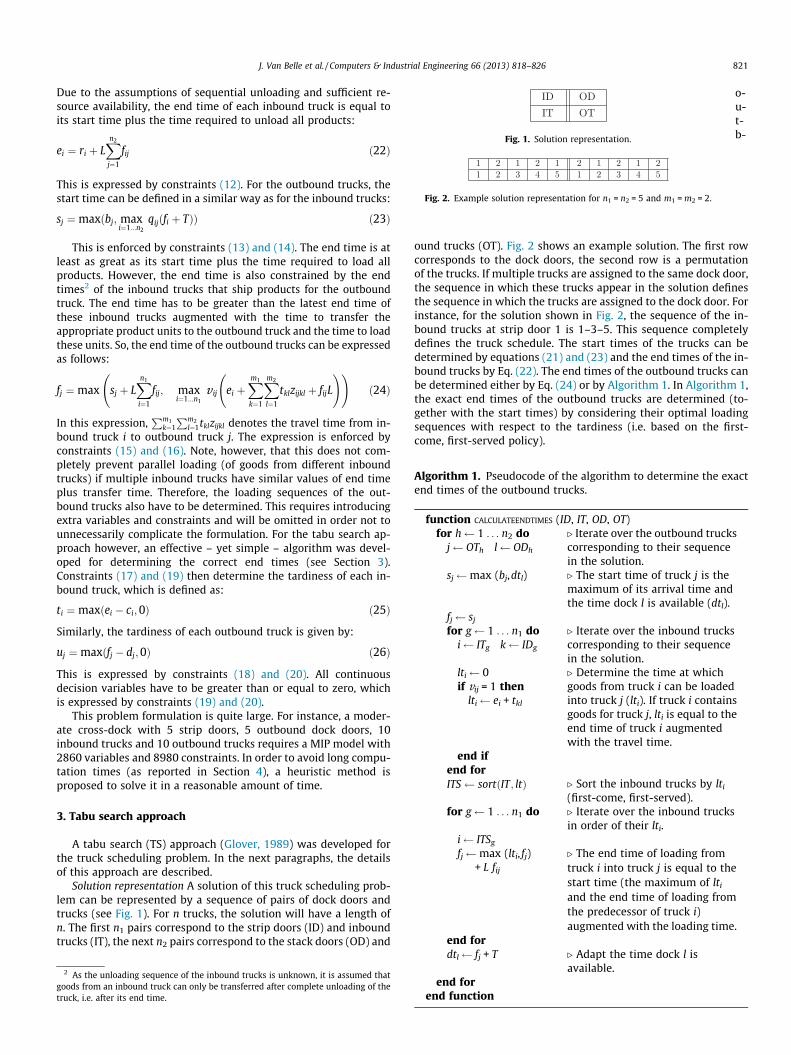
Fig. 1. Solution representation.
Fig. 2. Example solution representation for n1 = n2 = 5 and m1 = m2 = 2.
J. Van Belle et al. / Computers & Industrial Engineering 66 (2013) 818–826 821
Due to the assumptions of sequential unloading and sufficient re-source availability, the end time of each inbound truck is equal toits start time plus the time required to unload all products:
ei ¼ ri þ LXn2
j¼1
fij ð22Þ
This is expressed by constraints (12). For the outbound trucks, thestart time can be defined in a similar way as for the inbound trucks:
sj ¼maxðbj; maxi¼1...n2
qijðfi þ TÞÞ ð23Þ
This is enforced by constraints (13) and (14). The end time is atleast as great as its start time plus the time required to load allproducts. However, the end time is also constrained by the endtimes2 of the inbound trucks that ship products for the outboundtruck. The end time has to be greater than the latest end time ofthese inbound trucks augmented with the time to transfer theappropriate product units to the outbound truck and the time to loadthese units. So, the end time of the outbound trucks can be expressedas follows:
fj ¼max sj þ LXn1
i¼1
fij; maxi¼1...n1
v ij ei þXm1
k¼1
Xm2
l¼1
tklzijkl þ fijL
! !ð24Þ
In this expression,Pm1
k¼1
Pm2l¼1tklzijkl denotes the travel time from in-
bound truck i to outbound truck j. The expression is enforced byconstraints (15) and (16). Note, however, that this does not com-pletely prevent parallel loading (of goods from different inboundtrucks) if multiple inbound trucks have similar values of end timeplus transfer time. Therefore, the loading sequences of the out-bound trucks also have to be determined. This requires introducingextra variables and constraints and will be omitted in order not tounnecessarily complicate the formulation. For the tabu search ap-proach however, an effective – yet simple – algorithm was devel-oped for determining the correct end times (see Section 3).Constraints (17) and (19) then determine the tardiness of each in-bound truck, which is defined as:
ti ¼maxðei � ci;0Þ ð25Þ
Similarly, the tardiness of each outbound truck is given by:
uj ¼maxðfj � dj;0Þ ð26Þ
This is expressed by constraints (18) and (20). All continuousdecision variables have to be greater than or equal to zero, whichis expressed by constraints (19) and (20).
This problem formulation is quite large. For instance, a moder-ate cross-dock with 5 strip doors, 5 outbound dock doors, 10inbound trucks and 10 outbound trucks requires a MIP model with2860 variables and 8980 constraints. In order to avoid long compu-tation times (as reported in Section 4), a heuristic method isproposed to solve it in a reasonable amount of time.
3. Tabu search approach
A tabu search (TS) approach (Glover, 1989) was developed forthe truck scheduling problem. In the next paragraphs, the detailsof this approach are described.
Solution representation A solution of this truck scheduling prob-lem can be represented by a sequence of pairs of dock doors andtrucks (see Fig. 1). For n trucks, the solution will have a length ofn. The first n1 pairs correspond to the strip doors (ID) and inboundtrucks (IT), the next n2 pairs correspond to the stack doors (OD) and
2 As the unloading sequence of the inbound trucks is unknown, it is assumed thagoods from an inbound truck can only be transferred after complete unloading of thetruck, i.e. after its end time.
t
o-u-t-b-
ound trucks (OT). Fig. 2 shows an example solution. The first rowcorresponds to the dock doors, the second row is a permutationof the trucks. If multiple trucks are assigned to the same dock door,the sequence in which these trucks appear in the solution definesthe sequence in which the trucks are assigned to the dock door. Forinstance, for the solution shown in Fig. 2, the sequence of the in-bound trucks at strip door 1 is 1–3–5. This sequence completelydefines the truck schedule. The start times of the trucks can bedetermined by equations (21) and (23) and the end times of the in-bound trucks by Eq. (22). The end times of the outbound trucks canbe determined either by Eq. (24) or by Algorithm 1. In Algorithm 1,the exact end times of the outbound trucks are determined (to-gether with the start times) by considering their optimal loadingsequences with respect to the tardiness (i.e. based on the first-come, first-served policy).
Algorithm 1. Pseudocode of the algorithm to determine the exactend times of the outbound trucks.
function CALCULATEENDTIMES (ID, IT, OD, OT)
for h 1 . . . n2 do . Iterate over the outbound truckscorresponding to their sequencein the solution.
j OTh l ODh
sj max (bj,dtl)
. The start time of truck j is themaximum of its arrival time andthe time dock l is available (dtl).fj sj
for g 1 . . . n1 do
. Iterate over the inbound truckscorresponding to their sequencein the solution.i ITg k IDg
lti 0
. Determine the time at whichgoods from truck i can be loadedinto truck j (lti). If truck i containsgoods for truck j, lti is equal to theend time of truck i augmentedwith the travel time.if vij = 1 thenlti ei + tkl
end if
end for ITS sortðIT; ltÞ . Sort the inbound trucks by lti(first-come, first-served).
for g 1 . . . n1 do . Iterate over the inbound trucksin order of their lti.
i ITSgfj max (lti, fj)+ L fij
. The end time of loading fromtruck i into truck j is equal to thestart time (the maximum of lti
and the end time of loading fromthe predecessor of truck i)augmented with the loading time.
end for
dtl fj + T . Adapt the time dock l isavailable.
end forend function
822 J. Van Belle et al. / Computers & Industrial Engineering 66 (2013) 818–826
arrival times and the strip and stack doors are sorted by their aver-
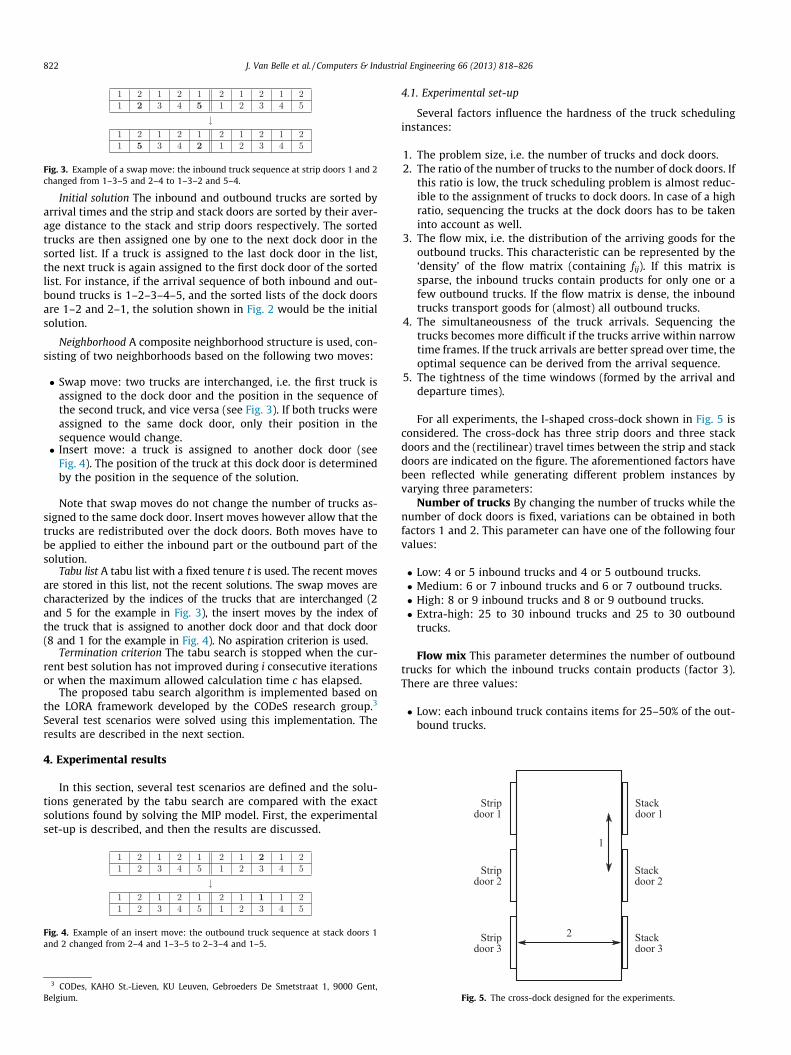
Fig. 3. Example of a swap move: the inbound truck sequence at strip doors 1 and 2
Initial solution The inbound and outbound trucks are sorted by
age distance to the stack and strip doors respectively. The sortedtrucks are then assigned one by one to the next dock door in thesorted list. If a truck is assigned to the last dock door in the list,the next truck is again assigned to the first dock door of the sortedlist. For instance, if the arrival sequence of both inbound and out-bound trucks is 1–2–3–4–5, and the sorted lists of the dock doorsare 1–2 and 2–1, the solution shown in Fig. 2 would be the initialsolution.
Neighborhood A composite neighborhood structure is used, con-sisting of two neighborhoods based on the following two moves:
� Swap move: two trucks are interchanged, i.e. the first truck isassigned to the dock door and the position in the sequence ofthe second truck, and vice versa (see Fig. 3). If both trucks wereassigned to the same dock door, only their position in thesequence would change.� Insert move: a truck is assigned to another dock door (see
Fig. 4). The position of the truck at this dock door is determinedby the position in the sequence of the solution.
Note that swap moves do not change the number of trucks as-signed to the same dock door. Insert moves however allow that thetrucks are redistributed over the dock doors. Both moves have tobe applied to either the inbound part or the outbound part of thesolution.
Tabu list A tabu list with a fixed tenure t is used. The recent movesare stored in this list, not the recent solutions. The swap moves arecharacterized by the indices of the trucks that are interchanged (2and 5 for the example in Fig. 3), the insert moves by the index ofthe truck that is assigned to another dock door and that dock door(8 and 1 for the example in Fig. 4). No aspiration criterion is used.
Termination criterion The tabu search is stopped when the cur-rent best solution has not improved during i consecutive iterationsor when the maximum allowed calculation time c has elapsed.
The proposed tabu search algorithm is implemented based onthe LORA framework developed by the CODeS research group.3
Several test scenarios were solved using this implementation. Theresults are described in the next section.
4. Experimental results
In this section, several test scenarios are defined and the solu-tions generated by the tabu search are compared with the exactsolutions found by solving the MIP model. First, the experimentalset-up is described, and then the results are discussed.
changed from 1–3–5 and 2–4 to 1–3–2 and 5–4.
Fig. 4. Example of an insert move: the outbound truck sequence at stack doors 1and 2 changed from 2–4 and 1–3–5 to 2–3–4 and 1–5.
3 CODes, KAHO St.-Lieven, KU Leuven, Gebroeders De Smetstraat 1, 9000 Gent,Belgium.
4.1. Experimental set-up
Several factors influence the hardness of the truck schedulinginstances:
1. The problem size, i.e. the number of trucks and dock doors.2. The ratio of the number of trucks to the number of dock doors. If
this ratio is low, the truck scheduling problem is almost reduc-ible to the assignment of trucks to dock doors. In case of a highratio, sequencing the trucks at the dock doors has to be takeninto account as well.
3. The flow mix, i.e. the distribution of the arriving goods for theoutbound trucks. This characteristic can be represented by the‘density’ of the flow matrix (containing fij). If this matrix issparse, the inbound trucks contain products for only one or afew outbound trucks. If the flow matrix is dense, the inboundtrucks transport goods for (almost) all outbound trucks.
4. The simultaneousness of the truck arrivals. Sequencing thetrucks becomes more difficult if the trucks arrive within narrowtime frames. If the truck arrivals are better spread over time, theoptimal sequence can be derived from the arrival sequence.
5. The tightness of the time windows (formed by the arrival anddeparture times).
For all experiments, the I-shaped cross-dock shown in Fig. 5 isconsidered. The cross-dock has three strip doors and three stackdoors and the (rectilinear) travel times between the strip and stackdoors are indicated on the figure. The aforementioned factors havebeen reflected while generating different problem instances byvarying three parameters:
Number of trucks By changing the number of trucks while thenumber of dock doors is fixed, variations can be obtained in bothfactors 1 and 2. This parameter can have one of the following fourvalues:
� Low: 4 or 5 inbound trucks and 4 or 5 outbound trucks.� Medium: 6 or 7 inbound trucks and 6 or 7 outbound trucks.� High: 8 or 9 inbound trucks and 8 or 9 outbound trucks.� Extra-high: 25 to 30 inbound trucks and 25 to 30 outbound
trucks.
Flow mix This parameter determines the number of outboundtrucks for which the inbound trucks contain products (factor 3).There are three values:
� Low: each inbound truck contains items for 25–50% of the out-bound trucks.
Fig. 5. The cross-dock designed for the experiments.
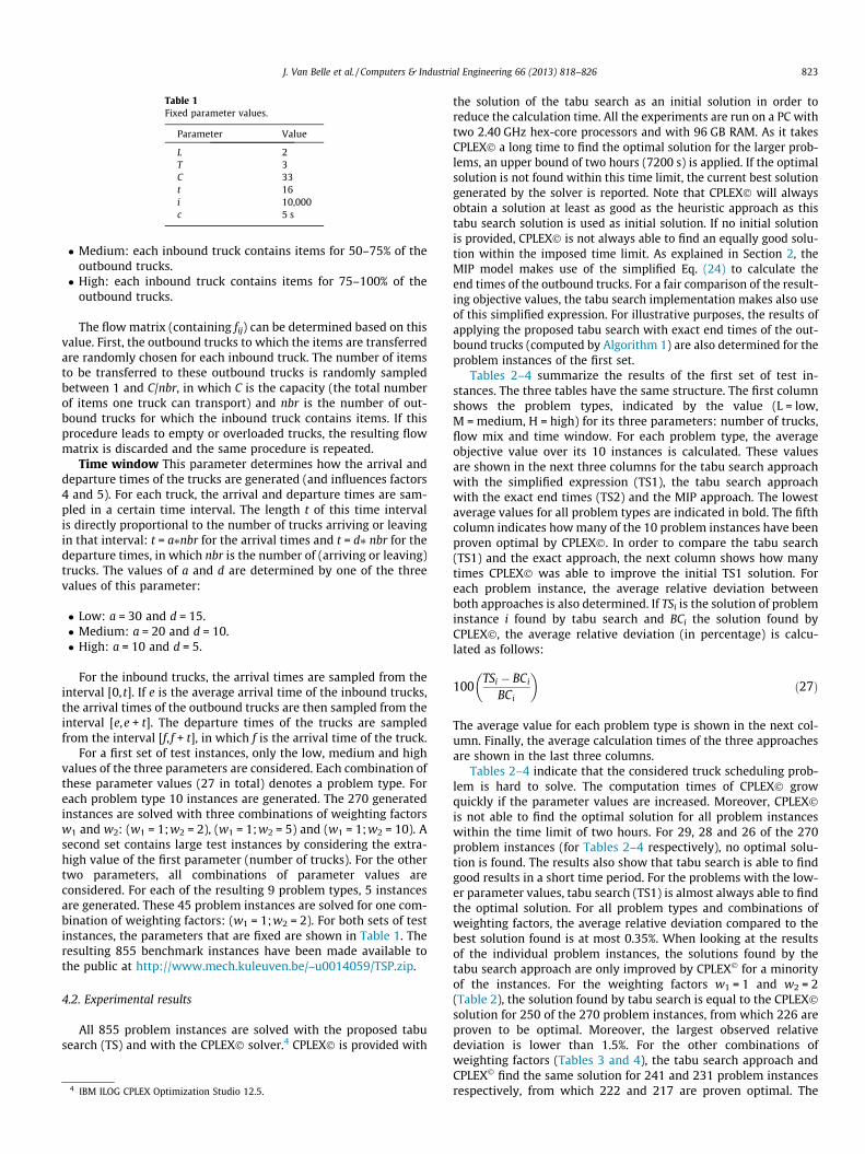
Table 1Fixed parameter values.
Parameter Value
L 2T 3C 33t 16i 10,000c 5 s
J. Van Belle et al. / Computers & Industrial Engineering 66 (2013) 818–826 823
� Medium: each inbound truck contains items for 50–75% of theoutbound trucks.� High: each inbound truck contains items for 75–100% of the
outbound trucks.
The flow matrix (containing fij) can be determined based on thisvalue. First, the outbound trucks to which the items are transferredare randomly chosen for each inbound truck. The number of itemsto be transferred to these outbound trucks is randomly sampledbetween 1 and C/nbr, in which C is the capacity (the total numberof items one truck can transport) and nbr is the number of out-bound trucks for which the inbound truck contains items. If thisprocedure leads to empty or overloaded trucks, the resulting flowmatrix is discarded and the same procedure is repeated.
Time window This parameter determines how the arrival anddeparture times of the trucks are generated (and influences factors4 and 5). For each truck, the arrival and departure times are sam-pled in a certain time interval. The length t of this time intervalis directly proportional to the number of trucks arriving or leavingin that interval: t = a⁄nbr for the arrival times and t = d⁄ nbr for thedeparture times, in which nbr is the number of (arriving or leaving)trucks. The values of a and d are determined by one of the threevalues of this parameter:
� Low: a = 30 and d = 15.� Medium: a = 20 and d = 10.� High: a = 10 and d = 5.
For the inbound trucks, the arrival times are sampled from theinterval [0, t]. If e is the average arrival time of the inbound trucks,the arrival times of the outbound trucks are then sampled from theinterval [e,e + t]. The departure times of the trucks are sampledfrom the interval [f, f + t], in which f is the arrival time of the truck.
For a first set of test instances, only the low, medium and highvalues of the three parameters are considered. Each combination ofthese parameter values (27 in total) denotes a problem type. Foreach problem type 10 instances are generated. The 270 generatedinstances are solved with three combinations of weighting factorsw1 and w2: (w1 = 1;w2 = 2), (w1 = 1;w2 = 5) and (w1 = 1;w2 = 10). Asecond set contains large test instances by considering the extra-high value of the first parameter (number of trucks). For the othertwo parameters, all combinations of parameter values areconsidered. For each of the resulting 9 problem types, 5 instancesare generated. These 45 problem instances are solved for one com-bination of weighting factors: (w1 = 1;w2 = 2). For both sets of testinstances, the parameters that are fixed are shown in Table 1. Theresulting 855 benchmark instances have been made available tothe public at http://www.mech.kuleuven.be/~u0014059/TSP.zip.
4.2. Experimental results
All 855 problem instances are solved with the proposed tabusearch (TS) and with the CPLEX� solver.4 CPLEX� is provided with
4 IBM ILOG CPLEX Optimization Studio 12.5.
the solution of the tabu search as an initial solution in order toreduce the calculation time. All the experiments are run on a PC withtwo 2.40 GHz hex-core processors and with 96 GB RAM. As it takesCPLEX� a long time to find the optimal solution for the larger prob-lems, an upper bound of two hours (7200 s) is applied. If the optimalsolution is not found within this time limit, the current best solutiongenerated by the solver is reported. Note that CPLEX� will alwaysobtain a solution at least as good as the heuristic approach as thistabu search solution is used as initial solution. If no initial solutionis provided, CPLEX� is not always able to find an equally good solu-tion within the imposed time limit. As explained in Section 2, theMIP model makes use of the simplified Eq. (24) to calculate theend times of the outbound trucks. For a fair comparison of the result-ing objective values, the tabu search implementation makes also useof this simplified expression. For illustrative purposes, the results ofapplying the proposed tabu search with exact end times of the out-bound trucks (computed by Algorithm 1) are also determined for theproblem instances of the first set.
Tables 2–4 summarize the results of the first set of test in-stances. The three tables have the same structure. The first columnshows the problem types, indicated by the value (L = low,M = medium, H = high) for its three parameters: number of trucks,flow mix and time window. For each problem type, the averageobjective value over its 10 instances is calculated. These valuesare shown in the next three columns for the tabu search approachwith the simplified expression (TS1), the tabu search approachwith the exact end times (TS2) and the MIP approach. The lowestaverage values for all problem types are indicated in bold. The fifthcolumn indicates how many of the 10 problem instances have beenproven optimal by CPLEX�. In order to compare the tabu search(TS1) and the exact approach, the next column shows how manytimes CPLEX� was able to improve the initial TS1 solution. Foreach problem instance, the average relative deviation betweenboth approaches is also determined. If TSi is the solution of probleminstance i found by tabu search and BCi the solution found byCPLEX�, the average relative deviation (in percentage) is calcu-lated as follows:
100TSi � BCi
BCi
� �ð27Þ
The average value for each problem type is shown in the next col-umn. Finally, the average calculation times of the three approachesare shown in the last three columns.
Tables 2–4 indicate that the considered truck scheduling prob-lem is hard to solve. The computation times of CPLEX� growquickly if the parameter values are increased. Moreover, CPLEX�is not able to find the optimal solution for all problem instanceswithin the time limit of two hours. For 29, 28 and 26 of the 270problem instances (for Tables 2–4 respectively), no optimal solu-tion is found. The results also show that tabu search is able to findgood results in a short time period. For the problems with the low-er parameter values, tabu search (TS1) is almost always able to findthe optimal solution. For all problem types and combinations ofweighting factors, the average relative deviation compared to thebest solution found is at most 0.35%. When looking at the resultsof the individual problem instances, the solutions found by thetabu search approach are only improved by CPLEX� for a minorityof the instances. For the weighting factors w1 = 1 and w2 = 2(Table 2), the solution found by tabu search is equal to the CPLEX�solution for 250 of the 270 problem instances, from which 226 areproven to be optimal. Moreover, the largest observed relativedeviation is lower than 1.5%. For the other combinations ofweighting factors (Tables 3 and 4), the tabu search approach andCPLEX� find the same solution for 241 and 231 problem instancesrespectively, from which 222 and 217 are proven optimal. The
Table 2The experimental results for the 27 problem types of set 1 with w1 = 1 and w2 = 2.
Problem type Objective value # MIP optimal # MIP better Relative dev. (%) Calculation time (s)
TS1 TS2 MIP TS1 TS2 MIP
L L L 518.300 528.299 518.300 10 0 0.000 0.164 0.445 0.089L L M 592.072 595.331 592.072 10 0 0.000 0.171 0.444 0.142L L H 837.478 856.069 837.478 10 0 0.000 0.155 0.420 0.200L M L 526.391 549.479 526.391 10 0 0.000 0.147 0.533 0.232L M M 654.059 682.388 654.059 10 0 0.000 0.153 0.547 0.276L M H 830.229 860.750 830.229 10 0 0.000 0.145 0.497 0.303L H L 684.285 698.018 684.285 10 0 0.000 0.167 0.796 0.504L H M 601.945 612.169 601.945 10 0 0.000 0.156 0.707 0.376L H H 957.740 974.641 957.740 10 0 0.000 0.152 0.659 0.651M L L 695.459 699.873 695.459 10 0 0.000 0.417 1.758 0.428M L M 962.622 974.925 962.622 10 0 0.000 0.425 1.701 0.604M L H 1236.073 1254.682 1236.073 10 0 0.000 0.407 1.670 3.029M M L 615.812 624.649 615.812 10 0 0.000 0.437 2.681 1.506M M M 1004.442 1021.004 1004.442 10 0 0.000 0.411 2.433 2.547M M H 1443.384 1461.398 1442.850 10 2 0.030 0.434 2.976 53.386M H L 875.440 884.003 875.140 10 1 0.035 0.426 3.318 6.321M H M 1150.058 1170.172 1149.558 10 1 0.050 0.421 3.134 22.655M H H 1704.644 1723.057 1703.419 10 1 0.065 0.506 3.889 501.419H L L 1033.019 1038.157 1032.119 10 2 0.148 0.876 4.375 1.159H L M 1197.026 1207.316 1197.026 10 0 0.000 0.846 4.466 249.205H L H 1859.446 1885.563 1859.044 7 1 0.025 1.040 4.866 3016.883H M L 1037.082 1041.362 1036.773 9 1 0.024 1.010 5.002 732.883H M M 1151.924 1155.059 1151.924 10 0 0.000 0.996 5.001 523.429H M H 1985.397 2006.045 1980.634 2 3 0.218 1.011 5.002 5844.611H H L 1281.025 1292.770 1279.053 9 4 0.189 1.018 5.009 1143.100H H M 1712.346 1729.040 1711.646 4 2 0.039 1.139 5.009 4629.849H H H 2437.626 2466.332 2436.826 0 2 0.035 1.025 5.009 7200.953
Table 3The experimental results for the 27 problem types of set 1 with w1 = 1 and w2 = 5.
Problem type Objective value # MIP optimal # MIP better Relative dev. (%) Calculation time (s)
TS1 TS2 MIP TS1 TS2 MIP
L L L 1076.750 1102.493 1076.750 10 0 0.000 0.165 0.448 0.066L L M 1217.282 1228.178 1217.282 10 0 0.000 0.163 0.450 0.143L L H 1839.085 1886.296 1839.085 10 0 0.000 0.157 0.432 0.170L M L 1014.146 1072.421 1014.146 10 0 0.000 0.149 0.540 0.242L M M 1354.048 1423.474 1354.048 10 0 0.000 0.157 0.548 0.267L M H 1798.656 1877.169 1798.656 10 0 0.000 0.149 0.515 0.292L H L 1387.713 1423.244 1387.713 10 0 0.000 0.168 0.815 0.424L H M 1212.213 1237.473 1212.213 10 0 0.000 0.156 0.712 0.425L H H 2076.650 2123.041 2076.650 10 0 0.000 0.154 0.687 0.521M L L 1345.736 1359.180 1345.736 10 0 0.000 0.447 1.865 0.419M L M 1989.142 2021.419 1988.242 10 1 0.047 0.430 1.783 0.713M L H 2680.817 2725.779 2680.817 10 0 0.000 0.431 1.856 3.054M M L 1126.519 1147.226 1125.319 10 1 0.068 0.437 2.810 1.408M M M 2088.537 2133.343 2088.537 10 0 0.000 0.425 2.564 4.436M M H 3152.726 3198.022 3152.396 10 1 0.008 0.448 2.926 193.110M H L 1728.035 1750.942 1728.035 10 0 0.000 0.434 3.284 5.546M H M 2399.145 2448.070 2396.945 10 2 0.074 0.431 3.287 26.075M H H 3748.651 3794.954 3743.348 9 2 0.142 0.491 4.091 1150.627H L L 2060.984 2072.287 2059.084 10 2 0.165 1.027 4.642 1.133H L M 2490.859 2517.736 2490.859 10 0 0.000 0.910 4.617 221.262H L H 4075.916 4130.299 4064.107 6 2 0.279 1.084 4.867 3770.478H M L 2011.945 2021.458 2010.545 10 2 0.076 1.065 5.001 172.269H M M 2321.451 2331.807 2320.651 9 1 0.042 1.058 5.002 847.884H M H 4367.173 4418.863 4352.298 3 3 0.293 1.080 5.002 5494.608H H L 2571.854 2603.297 2567.013 10 5 0.303 1.023 5.001 502.399H H M 3632.164 3674.632 3631.164 5 3 0.028 1.103 5.001 4487.891H H H 5428.291 5496.029 5420.664 0 4 0.144 1.020 5.001 7200.966
824 J. Van Belle et al. / Computers & Industrial Engineering 66 (2013) 818–826
relative deviations are now slightly higher but still smaller than2.6% for w1 = 1 and w2 = 5 and 2.9% for w1 = 1 and w2 = 10. Tabusearch is also very efficient. The solutions of all problem instancesare found in less than 2 s, and the average calculation time perproblem type is less than 1.2 s for all combinations of weightingfactors.
To prevent loading the outbound trucks in parallel, the secondtabu search implementation (TS2) makes use of Algorithm 1 todetermine the end times of the outbound trucks. This implies that
the objective values obtained with TS2 are at least as large as theoptimal objective values of the MIP model. Comparing the resultsof TS1 and the MIP approach shows that the average relativedeviation between the objective values of both is 1.6% for theresults in Table 2, with a maximum deviation of 12.5%. For Tables3 and 4, the average deviations are 1.9% and 2.1% respectivelyand the maximum deviations are 15.4% and 17.2%. This indicatesthat also TS2 is able to generate good quality results. The calcula-tion of the exact end times is however computationally more
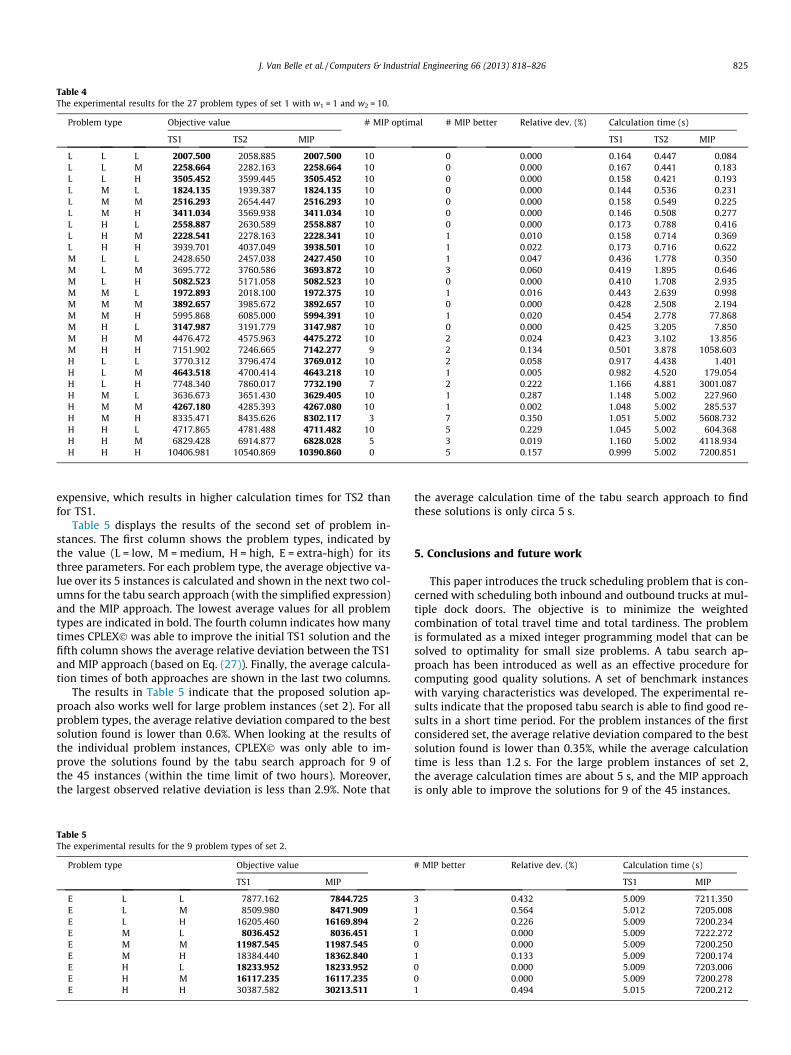
Table 4The experimental results for the 27 problem types of set 1 with w1 = 1 and w2 = 10.
Problem type Objective value # MIP optimal # MIP better Relative dev. (%) Calculation time (s)
TS1 TS2 MIP TS1 TS2 MIP
L L L 2007.500 2058.885 2007.500 10 0 0.000 0.164 0.447 0.084L L M 2258.664 2282.163 2258.664 10 0 0.000 0.167 0.441 0.183L L H 3505.452 3599.445 3505.452 10 0 0.000 0.158 0.421 0.193L M L 1824.135 1939.387 1824.135 10 0 0.000 0.144 0.536 0.231L M M 2516.293 2654.447 2516.293 10 0 0.000 0.158 0.549 0.225L M H 3411.034 3569.938 3411.034 10 0 0.000 0.146 0.508 0.277L H L 2558.887 2630.589 2558.887 10 0 0.000 0.173 0.788 0.416L H M 2228.541 2278.163 2228.341 10 1 0.010 0.158 0.714 0.369L H H 3939.701 4037.049 3938.501 10 1 0.022 0.173 0.716 0.622M L L 2428.650 2457.038 2427.450 10 1 0.047 0.436 1.778 0.350M L M 3695.772 3760.586 3693.872 10 3 0.060 0.419 1.895 0.646M L H 5082.523 5171.058 5082.523 10 0 0.000 0.410 1.708 2.935M M L 1972.893 2018.100 1972.375 10 1 0.016 0.443 2.639 0.998M M M 3892.657 3985.672 3892.657 10 0 0.000 0.428 2.508 2.194M M H 5995.868 6085.000 5994.391 10 1 0.020 0.454 2.778 77.868M H L 3147.987 3191.779 3147.987 10 0 0.000 0.425 3.205 7.850M H M 4476.472 4575.963 4475.272 10 2 0.024 0.423 3.102 13.856M H H 7151.902 7246.665 7142.277 9 2 0.134 0.501 3.878 1058.603H L L 3770.312 3796.474 3769.012 10 2 0.058 0.917 4.438 1.401H L M 4643.518 4700.414 4643.218 10 1 0.005 0.982 4.520 179.054H L H 7748.340 7860.017 7732.190 7 2 0.222 1.166 4.881 3001.087H M L 3636.673 3651.430 3629.405 10 1 0.287 1.148 5.002 227.960H M M 4267.180 4285.393 4267.080 10 1 0.002 1.048 5.002 285.537H M H 8335.471 8435.626 8302.117 3 7 0.350 1.051 5.002 5608.732H H L 4717.865 4781.488 4711.482 10 5 0.229 1.045 5.002 604.368H H M 6829.428 6914.877 6828.028 5 3 0.019 1.160 5.002 4118.934H H H 10406.981 10540.869 10390.860 0 5 0.157 0.999 5.002 7200.851
J. Van Belle et al. / Computers & Industrial Engineering 66 (2013) 818–826 825
expensive, which results in higher calculation times for TS2 thanfor TS1.
Table 5 displays the results of the second set of problem in-stances. The first column shows the problem types, indicated bythe value (L = low, M = medium, H = high, E = extra-high) for itsthree parameters. For each problem type, the average objective va-lue over its 5 instances is calculated and shown in the next two col-umns for the tabu search approach (with the simplified expression)and the MIP approach. The lowest average values for all problemtypes are indicated in bold. The fourth column indicates how manytimes CPLEX� was able to improve the initial TS1 solution and thefifth column shows the average relative deviation between the TS1and MIP approach (based on Eq. (27)). Finally, the average calcula-tion times of both approaches are shown in the last two columns.
The results in Table 5 indicate that the proposed solution ap-proach also works well for large problem instances (set 2). For allproblem types, the average relative deviation compared to the bestsolution found is lower than 0.6%. When looking at the results ofthe individual problem instances, CPLEX� was only able to im-prove the solutions found by the tabu search approach for 9 ofthe 45 instances (within the time limit of two hours). Moreover,the largest observed relative deviation is less than 2.9%. Note that
Table 5The experimental results for the 9 problem types of set 2.
Problem type Objective value
TS1 MIP
E L L 7877.162 7844.725E L M 8509.980 8471.909E L H 16205.460 16169.894E M L 8036.452 8036.451E M M 11987.545 11987.545E M H 18384.440 18362.840E H L 18233.952 18233.952E H M 16117.235 16117.235E H H 30387.582 30213.511
the average calculation time of the tabu search approach to findthese solutions is only circa 5 s.
5. Conclusions and future work
This paper introduces the truck scheduling problem that is con-cerned with scheduling both inbound and outbound trucks at mul-tiple dock doors. The objective is to minimize the weightedcombination of total travel time and total tardiness. The problemis formulated as a mixed integer programming model that can besolved to optimality for small size problems. A tabu search ap-proach has been introduced as well as an effective procedure forcomputing good quality solutions. A set of benchmark instanceswith varying characteristics was developed. The experimental re-sults indicate that the proposed tabu search is able to find good re-sults in a short time period. For the problem instances of the firstconsidered set, the average relative deviation compared to the bestsolution found is lower than 0.35%, while the average calculationtime is less than 1.2 s. For the large problem instances of set 2,the average calculation times are about 5 s, and the MIP approachis only able to improve the solutions for 9 of the 45 instances.
# MIP better Relative dev. (%) Calculation time (s)
TS1 MIP
3 0.432 5.009 7211.3501 0.564 5.012 7205.0082 0.226 5.009 7200.2341 0.000 5.009 7222.2720 0.000 5.009 7200.2501 0.133 5.009 7200.1740 0.000 5.009 7203.0060 0.000 5.009 7200.2781 0.494 5.015 7200.212
826 J. Van Belle et al. / Computers & Industrial Engineering 66 (2013) 818–826
Although various real-world details are taken into account,several others have not been considered (e.g. interchangeableproducts, limited storage capacity and internal congestion). Also,uncertainty and variability are not taken into account and theproblem is assumed to be static (while in practice trucks arrivelate, equipment fails, etc.). So, future research should incorporatethese issues in the truck scheduling problem in order to increasethe applicability.
The authors advocate another approach and will use the solutionobtained with the proposed tabu search approach as an input to alogistics execution system (LES) (Van Belle et al., 2011). This soft-ware system is responsible for the real-time execution of the logis-tic operations of the cross-dock. It is based on a self-organizing anddecentralized approach in order to improve the responsiveness andproactiveness and to handle changes and disturbances as business-as-usual. The LES ensures that the generated truck schedule can beexecuted in reality by accounting for omitted details and by react-ing to variations and disturbances. On the other hand, the LES canbenefit from the global view provided by a good quality truck sche-dule to improve its performance. So, the idea of the cooperation is tocombine the robustness and flexibility of the LES with the optimiza-tion of the organizational objectives by the presented schedulingapproach.Acknowledgements .
Acknowledgements
The authors would like to thank Wim Vancroonenburg andTony Wauters for their support with the implementation of thetabu search approach based on the LORA framework.
References
Arabani, A. R. B., Ghomi, S. M. T. F., & Zandieh, M. (2011). Meta-heuristicsimplementation for scheduling of trucks in a cross-docking system withtemporary storage. Expert Systems with Applications, 38, 1964–1979.
Bartholdi, J. J., III, & Gue, K. R. (2000). Reducing labor costs in an LTL crossdockingterminal. Operations Research, 48, 823–832.
Boysen, N. (2010). Truck scheduling at zero-inventory cross docking terminals.Computers & Operations Research, 37, 32–41.
Boysen, N., & Fliedner, M. (2010). Cross dock scheduling: Classification, literaturereview and research agenda. Omega, 38, 413–422.
Glover, F. (1989). Tabu search—Part I. ORSA Journal on Computing, 1, 190–206.Gue, K. R. (1999). The effects of trailer scheduling on the layout of freight terminals.
Transportation Science, 33, 419–428.McWilliams, D. L. (2009a). A dynamic load-balancing scheme for the parcel hub-
scheduling problem. Computers & Industrial Engineering, 57, 958–962.McWilliams, D. L. (2009b). Genetic-based scheduling to solve the parcel hub
scheduling problem. Computers & Industrial Engineering, 56, 1607–1616.McWilliams, D. L. (2010). Iterative improvement to solve the parcel hub scheduling
problem. Computers & Industrial Engineering, 59, 136–144.McWilliams, D. L., Stanfield, P. M., & Geiger, C. D. (2005). The parcel hub scheduling
problem: A simulation-based solution approach. Computers & IndustrialEngineering, 49, 393–412.
McWilliams, D. L., Stanfield, P. M., & Geiger, C. D. (2008). Minimizing the completiontime of the transfer operations in a central parcel consolidation terminal withunequal-batch-size inbound trailers. Computers & Industrial Engineering, 54,709–720.
Miao, Z., Lim, A., & Ma, H. (2009). Truck dock assignment problem with operationaltime constraint within crossdocks. European Journal of Operational Research, 192,105–115.
Oh, Y., Hwang, H., Cha, C. N., & Lee, S. (2006). A dock-door assignment problem forthe Korean mail distribution center. Computers & Industrial Engineering, 51,288–296.
Tsui, L. Y., & Chang, C.-H. (1990). A microcomputer based decision support tool forassigning dock doors in freight yards. Computers & Industrial Engineering, 19,309–312.
Tsui, L. Y., & Chang, C.-H. (1992). An optimal solution to a dock door assignmentproblem. Computers & Industrial Engineering, 23, 283–286.
Vahdani, B., & Zandieh, M. (2010). Scheduling trucks in cross-docking systems:Robust meta-heuristics. Computers & Industrial Engineering, 58, 12–24.
Van Belle, J., Saint Germain, B., Valckenaers, P., Van Brussel, H., Bahtiar, R., &Cattrysse, D. (2011). Intelligent products in the supply chain are merginglogistic and manufacturing operationsS. Bittanti, A. Cenedese, & S. Zampieri(Eds.). Preprints of the 18th IFAC world congress, 1596–1601.
Van Belle, J., Valckenaers, P., & Cattrysse, D. (2012). Cross-docking: State of the art.Omega, 40, 827–846.
Yu, W., & Egbelu, P. J. (2008). Scheduling of inbound and outbound trucks in crossdocking systems with temporary storage. European Journal of OperationalResearch, 184, 377–396.
Yu, V. F., Sharma, D., & Murty, K. G. (2008). Door allocations to origins anddestinations at less-than-truckload trucking terminals. Journal of Industrial andSystems Engineering, 2, 1–15.


![Maintenance Scheduling of Thermal Power Units in ... · evolutionary techniques, as genetic algorithm [6,7], simulated annealing [7,8], memetic algorithm [9], tabu search [7,10,11]](https://img.pdfslide.net/doc/110x75/5f3ba881e62c066b05646aee/maintenance-scheduling-of-thermal-power-units-in-evolutionary-techniques-as.jpg)