Embed Size (px)
Citation preview

A Techno-Commercial Assessment of Residential and Bulk
Battery Energy Storage
by
Aditya Nadkarni
A Thesis Presented in Partial Fulfillment
of the Requirements for the Degree
Master of Science
Approved February 2013 by the
Graduate Supervisory Committee:
George Karady, Chair
Kory Hedman
Raja Ayyanar
ARIZONA STATE UNIVERSITY
May 2013

i
ABSTRACT
Battery energy storage has shown a lot of potential in the recent past to be
effective in various grid services due to its near instantaneous ramp rates and
modularity. This thesis aims to determine the commercial viability of customer
premises and substation sited battery energy storage systems. Five different types
of services have been analyzed considering current market pricing of Lithium-ion
batteries and power conditioning equipment. Energy Storage Valuation Tool 3.0
(Beta) has been used to exclusively determine the value of energy storage in the
services analyzed. The results indicate that on the residential level, Lithium-ion
battery energy storage may not be a cost beneficial option for retail tariff
management or demand charge management as only 20-30% of the initial
investment is recovered at the end of 15 year plant life. SRP’s two retail Time-of-
Use price plans E-21 and E-26 were analyzed in respect of their ability to increase
returns from storage compared to those with flat pricing. It was observed that
without a coupled PV component, E-21 was more suitable for customer premises
energy storage, however, its revenue stream reduces with addition to PV. On the
grid scale, however, with carefully chosen service hierarchy such as distribution
investment deferral, spinning or balancing reserve support, the initial investment
can be recovered to an extent of about 50-70%. The study done here is specific to
Salt River Project inputs and data. Results for all the services analyzed are highly
location specific and are only indicative of the overall viability and returns from
them.

ii
ACKNOWLEDGMENTS
I would like to extend my sincere thanks to Prof. Dr. G.G. Karady for providing
me with an opportunity to test my abilities in academic research and also guiding
me throughout the course of this project. The freedom for ideas and innovation
that he allowed, truly helped in exploring wonderful avenues of engineering and
research in general. I would also like to take this opportunity to thank Dr. Raja
Ayyanar and Dr. Kory Hedman for taking time to serve as my defense committee
members and offering their valuable inputs.
The work was funded by SRP and EPRI and I am grateful for their continued
interest in the project. My thanks to Mr. Ken Alteneder at SRP for promptly
responding to my research related queries and providing essential data from time
to time. The work would not have reached its meaningful conclusion without the
support of Mr. Ben Kaun and Ms. Stella Chen, both from EPRI, who played a big
role in getting me work on their ESVT 3.0 (beta) software and were also
extremely prompt with their inputs. I would also like to thank a number of other
experts from SRP and EPRI who provided me with useful insights into the work.
Finally, I would like to thank my colleagues in the power engineering department
at ASU and friends from school and undergraduate college for being a source of
constant inspiration, support and encouragement. Again, my heartfelt gratitude to
my family and relatives for praying for my well-being and success.

iii
TABLE OF CONTENTS
Page
LIST OF TABLES ............................................................................................... v
LIST OF FIGURES ........................................................................................... vii
NOMENCLATURE ............................................................................................ x
CHAPTER
1 INTRODUCTION ............................................................................ 1
1.1 Background .......................................................................... 1
1.2 Motivation ............................................................................ 2
1.3 Research objectives ............................................................... 3
1.4 Organization of thesis ........................................................... 4
2 LITERATURE REVIEW ................................................................. 6
2.1 Battery energy storage – A functional overview ..................... 6
2.2 Lithium-ion batteries and factors governing their cost ............ 8
2.3 Indoor testing methods for battery cycling ........................... 11
2.4 Battery energy storage in end-user specific services ............. 12
2.5 Battery energy storage in utility specific services ................. 15
2.6 Scope for further research ................................................... 17
3 DATA PREPARATION AND MODELING BESS ......................... 19
3.1 Description of simulation models ........................................ 19
3.2 Residential tariff structure and load profile .......................... 26
3.3 Technical input and output indices....................................... 30

iv
CHAPTER Page
3.4 Financial input and output indices ....................................... 33
4 COST ANALYSIS OF 2KW/4.4 HOUR BESS IN 40% PEAK
SHAVING SCENARIO .................................................................. 37
4.1 Introduction ........................................................................ 37
4.2 Analysis of residential 40% peak-shaving using BESS ......... 37
4.3 PV system capacity curtailment using energy storage ........... 49
4.4 An accelerated testing method for photovoltaic duty batteries
……………………………………………………………………………………………………….50
5 SERVICE SPECIFIC COST-BENEFIT ANALYSIS OF BESS ....... 62
5.1 Introduction ........................................................................ 62
5.2 Service – I: Retail TOU Energy Time-shift .......................... 63
5.3 Service – II: Retail Demand Charge Management ................ 75
5.4 Service – III: Distribution Investment Deferral .................... 81
5.5 Service – IV: Spinning Reserve Support and Energy Arbitrage
....................................................................................................................................................................93
6 CONCLUSION AND SCOPE FOR FUTURE RESEARCH……………...98
REFERENCES ................................................................................................ 101
APPENDIX
A MATLAB Code for calculating energy storage dispatch…………………...103
B SunVerge SIS 2.0 datasheet……………………………………………………………………115
C Excel spreadsheet for calculating storage system life-cycle cost…..117

v
LIST OF TABLES
Table Page
2.1 Cost estimate of Lithium ion batteries by EPRI [11] ................................... 10
2.2 Cost estimates of used Lithium ion batteries by ORNL .............................. 11
2.3 Utility Time-of-Use tariffs (only summer).................................................. 14
2.4 Typical operation periods of batteries for grid services ............................... 16
3.1 Solar panel thermal parameters .................................................................. 21
3.2 PVI-4.2-OUTD-US inverter specifications [31] ......................................... 21
3.3 OpenDSS storage element model parameters ............................................. 26
3.4 SRP tariff plans studied .............................................................................. 27
4.1 Battery storage and tariff parameters .......................................................... 40
4.2 Cost indices of PV system .......................................................................... 47
4.3 Cost indices of storage system ................................................................... 48
4.4 Results for 40% peak shaving system with Pload = 2 kW ............................ 48
4.5 Test battery parameters .............................................................................. 54
4.6 Summary on monthly battery cycling performance .................................... 61
5.1 Load management applications studied ...................................................... 62
5.2 Input parameters for the current case .......................................................... 64
5.3 Cost-benefit results with 2 kW/4.4 hour storage ......................................... 66
5.4 Cost benefit results for E-21 customer with 2kW/3 hour storage ................ 66
5.5 Input battery and load parameter specifications .......................................... 70
5.6 Cost-benefit results for Pload_peak = 2 kW .................................................... 72
5.7 Cost-benefit results for Pload_peak = 3 kW .................................................... 72
5.8 Input indices for demand charge management service ................................ 77

vi
Table Page
5.9 Demand-charge management results for E-36 and E-32 ............................. 79
5.10 Input indices for distribution investment deferral service.......................... 84
5.11 Description of OpenDSS model of SRP residential feeder ........................ 85
5.12 Results for distribution investment deferral at substation .......................... 88
5.13 Investment deferral results for 1MW, 4hour storage, 2% load growth in year
3 ........................................................................................................................ 90
5.14 Comparison of benefits from different grid services ................................. 97

vii
LIST OF FIGURES
Figure Page
1.1 Laurel mountain 32 MW/15 minute Lithium ion battery storage for wind
farm support ........................................................................................................ 2
2.1 Block diagram of rooftop PV and energy storage system ............................. 6
2.2 Lithium ion battery cell reactions ................................................................. 8
2.3 Summer hourly profile of battery cycling and demand ............................... 13
3.1 OpenDSS PV system model ....................................................................... 20
3.2 Variation of inverter efficiency with its power output................................. 22
3.3 OpenDSS PV system output in per unit in average (left) and hourly (right)
form .................................................................................................................. 23
3.4 Storage model used in OpenDSS ................................................................ 24
3.5 Seasonal TOU tariff charges for E-21 ........................................................ 27
3.6 Seasonal TOU tariff charges for E-26 ........................................................ 28
3.7 Seasonal demand-charge tariff charges for E-36 and E-32 .......................... 28
3.8 Seasonal TOU tariff charges for E-32 ........................................................ 29
3.9 Average seasonal loadshapes for E-21(Left) and E-26(Right) .................... 29
4.1 Block diagram of battery assisted PV system simulated (Left) and Sunverge
SIS (Right) ........................................................................................................ 38
4.2 Daily excess kWh generation from a 3 kW PV system serving a 2 kW peak
demand .............................................................................................................. 41
4.3 Customer 8760 net demand for 40% peak-shave target and variable PV sizes
for E-26 tariff .................................................................................................... 42
4.4 Annual net load with 2 kW demand peak, 40% peak-shave target and
variable PV sizes for E-21 tariff ......................................................................... 44
4.5 Summer hourly profiles in loadshape mode for E-21 (Left) and E-26 (Right)
.......................................................................................................................... 44

viii
Figure Page
4.6 Monthly and annual revenue with respect to E-26 tariff ............................. 45
4.7 Monthly and annual revenue earnings/bill savings with E-21 tariff............. 46
4.8 Summer monthly electricity bill comparison with Grid – I system.............. 50
4.9 Hourly PV, demand and battery cycling profile for summer ....................... 52
4.10 Testing experimental setup in the laboratory ............................................ 53
4.11 Comparison of reproduced and expected battery cycling profiles ............. 58
4.12 Average charging and discharging power observed in each step of cycling
.......................................................................................................................... 59
4.13 Daily Wh profile of battery cycling ........................................................... 60
5.1 Dispatch hierarchy map for ESVT – 3 Beta (Source ESVT – 3 Beta Manual)
.......................................................................................................................... 63
5.2 Summer hourly storage dispatch and net load for E-21 and E-26 customers 65
5.3 PVal of monthly savings for E-21 and E-26 tariffs ..................................... 67
5.4 Annual savings for E-21 and E-26 tariffs with 2kW/4.4 hour storage ......... 67
5.5 Summer Net load profile for E-21(Left) and E-26(Right) ........................... 71
5.6 Monthly benefits for 3 kW peak load with E-21(Left) and E-26(Right) tariffs
.......................................................................................................................... 73
5.7 Annual revenue for E-21(Left) and E-26(Right) tariffs with different PV
sizes .................................................................................................................. 73
5.8 E-21 and E-26 storage dispatch and hourly retail pricing ............................ 74
5.9 8760 load profile for E-36 and E-32 tariffs ................................................. 78
5.10 Summer dispatch for demand charge management with E-36 ................... 79
5.11 Net demand with demand charge management before and after storage
dispatch ............................................................................................................. 80
5.12 Hourly market price of electricity at Palo Verde (2011) ........................... 84

ix
Figure Page
5.13 OpenDSS circuit plot of residential feeder modeled ................................. 86
5.14 Annual and summer daily substation load ................................................ 87
5.15 Substation (Top) and residential feeder head (Bottom) demand before and
after storage dispatch ......................................................................................... 89
5.16 Battery SoC and number of dispatch days in year 3 .................................. 90
5.17 Storage dispatch comparison between services I and III ........................... 91
5.18 Net substation demand profile before and after storage dispatch ............... 92
5.19 Hourly value for holding spinning reserve capacity to SRP ...................... 95

x
NOMENCLATURE
AEP American Electric Power
BESS Battery Energy Storage System
DoD Depth of discharge
DoE Department of Energy
EPRI Electric Power Research Institute
ESVT Energy Storage Valuation Tool
NPV Net present value
NREL National Renewable Energy Laboratory
OpenDSS Opensource Distribution System Simulator
ORNL Oak Ridge National Laboratory
PCS Power conditioning subsystem
PV Photovoltaic
PVal Present value
SMUD Sacramento Municipal Utility District
SoC State of charge
SRP Salt River Project
WECC Western Electricity Coordinating Council
1
Chapter 1. INTRODUCTION
1.1 Background
Role of Battery Energy Storage System (BESS) in customer premises
services as well as grid level ancillary services is increasingly being analyzed
today. With growing interest in smart grids, modular energy storage, associated
automation and communication networking are expected to be at the very heart of
this allied research. Lithium-ion technology is being seen as a promising battery
storage option for residential (2-5 kW), commercial (10-50 kW), community
storage (> 50 kW) and bulk storage (> 100 kW) systems. According to DOE’s
Energy Storage Database (beta), about five Lithium-ion battery bulk storage
projects are currently operational in the United States while three are under
construction [1]. Some of these are utility owned while others are demonstration
projects or third party initiatives. On a residential scale, integrated modules of
batteries and power conditioning systems are being used in conjunction with
existing grid connected rooftop solar photovoltaic systems or independently.
Energy storage services of interest to end-users include retail Time-of-Use energy
charge management, demand charge management, power reliability while utility
owned BESS benefits stem from annual substation peak-shaving, possible
frequency regulation, service reserve capacity, spinning reserve support and
voltage support.
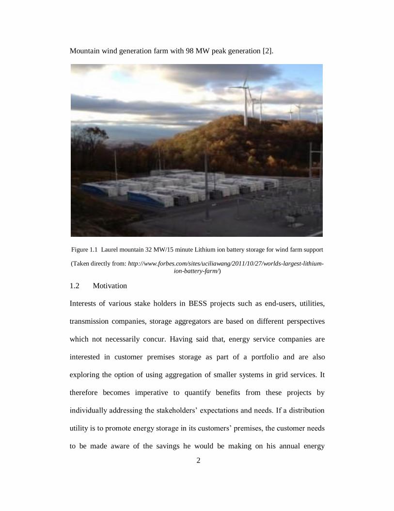
Fig. 1.1 shows one of the largest Lithium ion energy storage facilities deployed by
AES Corp for frequency regulation and ramping services in the vicinity of Laurel
2
Mountain wind generation farm with 98 MW peak generation [2].
Figure 1.1 Laurel mountain 32 MW/15 minute Lithium ion battery storage for wind farm support
(Taken directly from: http://www.forbes.com/sites/uciliawang/2011/10/27/worlds-largest-lithium-
ion-battery-farm/)
1.2 Motivation
Interests of various stake holders in BESS projects such as end-users, utilities,
transmission companies, storage aggregators are based on different perspectives
which not necessarily concur. Having said that, energy service companies are
interested in customer premises storage as part of a portfolio and are also
exploring the option of using aggregation of smaller systems in grid services. It
therefore becomes imperative to quantify benefits from these projects by
individually addressing the stakeholders’ expectations and needs. If a distribution
utility is to promote energy storage in its customers’ premises, the customer needs
to be made aware of the savings he would be making on his annual energy

3
consumption. Demonstration projects headed by distribution companies with
technical expertise from other research organizations or university research are a
useful way for increasing the penetration of distributed generation or storage on
the grid. Also, advantages to the utility and grid impact of dispatching fleet of
storage devices need to be understood simultaneously. Also, in some cases, utility
owned bulk energy storage initiatives could be more suitable to large scale
renewable capacity firming and ancillary grid service applications. An up-to-date
cost benefit study is undoubtedly one of the major screening criteria for BESS
projects and also a benchmark for future investments in the same technology. As
established, the BESS projects are highly location and service sensitive in nature,
which needs to be factored into these cost studies. The third party ownership of
customer premises systems perspective has not been addressed in this study.
At the battery level, it becomes crucial to understand the cycling capacity of any
particular battery chemistry when put to service in the field. Batteries could lose
capacity very fast and be rendered unsuitable with frequent roundtrips. Battery
replacement costs form a substantial part of the lifetime investment into a BESS
project. Laboratory testing of batteries by creating a field-like environment could
be a cheap yet effective way of studying their cycling behavior over a period of
time.
1.3 Research objectives
The principle objectives of this thesis address the following topics related to
BESS. The utility data used in the analysis pertains to Salt River Project (SRP).

4
To quantify life-cycle costs and returns from a 2 kW/4.4 hour Lithium-ion
BESS to residential customers in a 40 % peak-shaving application involving
suitably sized solar photovoltaic (PV) component
Develop and test a prototype Lithium-ion battery in an accelerated manner
under a cycling pattern similar to that observed in typical grid-connected PV
system
Using the Energy Storage Valuation Tool (ESVT – 3 (Beta)), perform a
life-cycle cost study and analyze cycling behavior of a 2 kW/4.4 hour Lithium-ion
BESS for the following services
1. Retail Time-of-Use Energy Shift with and without PV system component
2. Demand charge management
Using the Energy Storage Valuation Tool (ESVT – 3 (Beta)) and
OpenDSS, quantify and compare annual substation investment deferral benefits to
utility from
1. 0.5 MW, 1 MW distributed storage on the distribution grid
2. 0.5 MW, 1 MW bulk energy storage near substation
Provide feedback to EPRI on ESVT – 3 (Beta)
1.4 Organization of thesis
The thesis is spanned across five principle chapters. Chapter 1 has presents the
motivation behind this study and enlisted the principle objectives concerning
BESS that will be addressed in the subsequent chapters. Chapter 2 presents a
literature review on various topics dealing with customer premises and bulk

5
energy storage systems on the grid and the research that has been done or still
underway. In Chapter 3, various simulation models, sample data and terminology
used in the thesis to model BESS are explained in detail. In Chapter 4, a detailed
cost analysis is developed for the proposed BESS in peak shaving application.
Also, an accelerated laboratory testing procedure is proposed thereafter for
Lithium-ion batteries in rooftop photovoltaic applications. Chapter 5 brings out
the results of the cost-benefit analysis of three BESS services namely, Retail TOU
energy shift, demand charge management and distribution investment deferral.
Finally, suitable conclusions drawn from the study are given in Chapter 6 along
with the scope for future research in this domain. The simulation program codes
and important data used are listed in Appendices.

6
Chapter 2. LITERATURE REVIEW
2.1 Battery energy storage – A functional overview
Battery Energy Storage System (BESS) is an integrated system of battery storage
unit, power conditioning and thermal management subsystem power conditioning
and thermal management subsystem, power conditioning and thermal
management subsystem, medium and low voltage switchgear together with
automation equipment in an enclosure [3]. BESS in a rooftop Photovoltaic system
(PV) provides a means of storing excess of solar energy during daytime for its use
later in the day when the sun ceases to shine. This use can pertain to shaving
evening peak demand and also as a source of backup power. If used independent
of PV, they are charged from the grid. SolarCity, a leading solar service provider,
depicts a similar but typical rooftop PV system in Fig. 2.1. [4]. The system
components include PV system, Battery unit, Inverter, Electrical panel/Utility
meter and Grid connection.
Figure 2.1 Block diagram of rooftop PV and energy storage system
(Adapted from SolarCity website, http://www.solarcity.com/residential/energy-storage.aspx)

7
At the core of battery energy storage system is the Power Conditioning System
(PCS) providing bidirectional power conversion. When the battery is charging
from the grid, the voltage source converter acts a rectifier and acts as an inverter
when the battery discharges to the load. Supply of reactive power can be
controlled through converter duty cycle control to cater to the reactive power
needs of the system, if employed for. Reactive power control could allow greater
degree of variable generation penetration on the grid if multitude of such systems
is present on the grid. BESS for most practical purposes can be seen as a voltage
source behind a reactance [5]. The generated voltage and power can be
completely controlled within the limits of converter. BESS can operate in all four
quadrants of real and reactive power generation and absorption due to its ability to
control the phase angle of current relative to the terminal voltage. BESS and PCS
together can also be modeled such that the system as a whole is identical in
principle to a rotating synchronous machine attached to a large inertia and prime
mover which can supply and absorb energy within its capacity. Battery
management system (BMS) serves as the brain for BESS. It monitors and
regulates battery voltage, temperature and current to their optimum. Regulation of
these critical battery parameters is of utmost importance to extend the battery life
and enhance overall system reliability. Advanced BMS systems have a wired as
well as wireless communication setup for remote monitoring and analysis or
SCADA.

8
2.2 Lithium-ion batteries and factors governing their cost
There are different types of battery chemistries each with different power, energy
and safety features. However, for the purpose of this study Lithium-ion chemistry
was considered.
Lithium ion batteries
Lithium provides largest specific energy per unit weight providing high energy
densities with lithium metal anode. However, during early research with this
configuration, the battery was seen to be unstable and on some instances highly
inflammable. This in effect made the non-metallic Lithium ion (Li-ion) chemistry
more suitable and commercially popular. The nominal voltage per Li-ion cell is
3.7 V and has a flat discharge profile. In Lithium ion (Cobalt Oxide) batteries, the
Lithium Cobalt Oxide forms the positive electrode and highly crystalline carbon
acts as a negative electrode. During charging, Lithium metal in the positive
terminal gets ionized and moves along the negative electrode. During discharge,
ionized Lithium recombines with the Cobalt Oxide at the positive terminal. Fig.
2.2 shows principle cell reactions taking place in a Lithium Cobalt Oxide battery
[6]. Here n denotes the number of molecules in a cell reaction.
At position electrode, LiCoO2 Lin CoO2 + n Li+ + n e
-
At negative electrodde, C + n Li+ + n e
- CLin
Figure 2.2 Lithium ion battery cell reactions
(Taken directly from [6])

9
Lithium manganese oxide (LiMn2O4) batteries have high current carrying
capacity and are increasingly being used for PHEV and grid storage applications.
Factors governing Lithium ion battery costs
Many cost models have been developed to quantify the economic feasibility of
using these batteries for stationary storage. Yet, there is very little comprehensive
literature on the application specific economic assessment of Lithium ion
batteries. The Argonne National Lab model for determining Li-ion battery
manufacturing cost discusses some of the critical factors which determine Li-ion
battery costs in PHEV applications [7].
Cost in dollars ($) per unit of battery charge/discharge rate ($/kWRated) and
storage capacity ($/kWhRated) are the two most important indices used to specify
the cost of Li-ion batteries. For stationary storage purposes, depending on the
applications, energy and power requirements from battery storage vary. For
example, in power quality, frequency regulation, load following, battery discharge
rate is extremely critical to supply fluctuations in demand occurring in a span of
seconds or less. In services such as backup power, energy time-shift, more
discharge hours (three to four) at the rated kW are desired.
On a micro-scale, power and energy extracted from the battery are directly related
to the cell area and electrode thickness respectively. Batteries with high power to
energy ratio have lower material cost. Number of cells also makes the cost vary
in proportion. With more number of cells having lower terminal voltages,
excessive cycling, production and testing costs incur. In essence, the cost of a
battery pack is an aggregation of costs incurred in building a cell, building a

10
module with a number of cells and building a pack with a number of modules.
Each stage requires added hardware assembly costs [7, 8]. In a broad perspective,
Lithium ion battery costs are primarily specific to the chemistry, internal electrode
design, cell area and to a lesser extent to battery capacity.
Recent cost estimate studies
EPRI’s recent white paper on Energy Storage Technology Options stands out as
one of the most elucidative comprehensions of current trends in the energy
storage industry [9]. The cost estimates presented therein have been referred to in
the thesis. Table 2.1 gives the $/kWh values of Lithium-ion batteries employed in
various energy storage services. The cost estimates have been derived from alteast
three battery vendors. The entire survey included more than 50 companies
manufacturing batteries of different chemistries. The wide range of cost for a
particular application arises from the upper and lower storage sizing limits,
different vendor assumptions on margin, production level and level of maturity.
An update to these cost estimates is given in [10]. It quantifies the storage unit
costs in terms of $/kW for the PCS element and $/kWh for the storage element.
Table 2.1 Cost estimate of Lithium ion batteries by EPRI [9]
Service Cost range of Lithium ion storage ($/kWh)
Frequency regulation 4340-6200
T&D grid support 900-1700
Community energy storage 950-3600
Residential energy management 800-2250

11
Also, Oak Ridge National Laboratory (ORNL) recently conducted an economic
analysis of deploying used batteries in power system applications [11]. Their
research evaluated life-cycle performance benefits for various services from
customer premises to substations. Table 2.2 enlists some of the principle services
and associated costs as a summary. Although the costs correspond to used
Lithium-ion batteries, they serve as a reasonable benchmark with costing studies
of battery energy storage.
Table 2.2 Cost estimates of used Lithium ion batteries by ORNL
Service Size requirement
(MW, MWh)
ORNL cost estimate
(Million $)
Energy time-shift 1, 5 1.8
Load following 1, 3 1.2
Voltage support 1, 0.5 0.274
Distribution upgrade
deferral
1, 4 1.5
Demand charge
management
0.2, 1 0.368
Renewable energy time
shift
0.001, 0.004 0.0015
2.3 Indoor testing methods for battery cycling
Testing of batteries is an important step in evaluating their cycling proficiency
over their prescribed life-time. Methods of testing however may vary depending

12
on the service the battery is employed in and also on the battery chemistry. Life-
cycle testing of stationary battery cycling tests were carried out in [12] for a
typical household in Arizona in order to have a long term perspective on the
battery performance from the actual field testing. Similar field testing of batteries
generally takes a long time (3-5 years) for the results to be available. An indoor
testing method closely replicating a PV system could therefore be desirable for
accelerated, flexible and controllable assessment of battery sizing and savings
from its operation [13-17]. In the recent past, Agilent Technologies’s ‘Solar
Array Simulator’ or SAS has been used as a laboratory substitute for PV panels
for matching batteries to PV panel peak rating in stand-alone applications [16-17].
A design of Stand-alone system in Malaysia with real time solar data is discussed
in [18] while in [19], a smart charge technique for reducing electricity bills is
discussed although without a PV element. However, in all these indoor methods,
actual month long experimental verification of battery cycling with regards to
seasonal variations has not been performed. Also, no particular charging and
discharging strategies in response to the retail tariff plans were addressed.
2.4 Battery energy storage in end-user specific services
In recent years, distribution utilities have restructured their retail electricity
pricing to use it as a tool to manage load. The time-of-Use (TOU) retail electricity
tariff structures offered by utilities are particularly directed at discouraging end-
users to increase their demand for electricity during distribution substation peak.
Customer premises energy storage makes use of the price differential between on-
peak and off-peak prices to offer benefits to the owners in the form of savings on

13
their monthly electricity bill. Greater proportion of summer peak load in the US
desert southwest is air conditioning. Such seasonal peculiarities need to be
reflected as closely as possible in the annual customer load shapes. In urban
residential Arizona locales such as the Phoenix Metropolitan, peak PV output and
daily demand peak are non-coincidental as shown in Fig. 2.3 [20].
Figure 2.3 Summer hourly profile of battery cycling and demand
In addition, utilities apply demand charges on commercial or industrial customers
whose kW demand during on-peak hours exceeds a predefined kW threshold. In
[21], impact of utility retail tariff structure on economics of domestic PV systems
has been addressed. The study is based on analysis of 55 different rate structures
from more than 25 cities. It was concluded that TOU rates are more beneficial to a
PV system compared to flat tariff structure based on correlation between peak
pricing and PV production, peak and off-peak price differential. Several net
metering policy riders are also offered by utilities, however they are not widely
pervasive as yet. In this, customers with rooftop PV are compensated for the

14
amount of power they supply the grid due to excess production. In some cases, it
allows customers to fully compensate for their electricity bills but does not pay
them for any supply to the grid after they have fully compensated for their
monthly bill; while in some cases as with Salt River Project (SRP), the annual net
energy fed to the grid is valued by the average market on-peak wholesale price at
Palo-Verde [22]. With regards to demand charge riders, PV owners whose
demand peaks in the afternoon are expected to get maximum benefits. For those it
does not, energy storage can prove to be a valuable proposition. Table 2.3 is a list
of various retail TOU tariffs offered by utilities, their on-peak hours and on-peak
charges.
Table 2.3 Utility Time-of-Use tariffs (only summer)
Name of utility On-peak
hours
On-peak
price ($/kWh)
Off-peak price
($/kWh)
PG&E (A1) 1 PM – 6 PM 0.23 0.185
SCE (8 CPP sec) 1 PM – 6 PM 0.12 0.062
SG&E (AL) 12 PM – 6 PM 0.12 0.074
SMUD (GS) 3 PM – 8 PM 0.15 0.096
SRP (E-26) 2 PM – 8 PM 0.19 0.068
APS (7 PM –
Noon)
12 PM – 7 PM 0.216 0.0541
A Sandia report on energy storage market potential assessment for DOE energy
storage program compares benefits from customer premises storage [23]. Retail
TOU tariffs play a significant role in deciding the returns from a storage

15
investment for these applications. The report’s assessment of profitability of
similar services to small scale users (< 10 kW) is however not quite encouraging.
Same is the case with demand charge management for small users. Benefits from
demand charge management are further lowered if a utility levies facility charges
on the customer. For large customers (>50 kW), synergies with other storage
services could yield higher benefits. Although savings on annual electricity bills
form the biggest chunk of end-user benefits, there are other benefits too such as
those from power quality and reliability improvements, which have not been
addressed in this study explicitly.
2.5 Battery energy storage in utility specific services
Use of battery energy storage in grid applications ranging from ancillary services
like spinning reserve support, frequency regulation to renewable integration and
peak shaving have been addressed in [24]. This study conducted by General
Electric (GE) recognizes the limitations in justifying investments in batteries for
grid services, however, it also concedes that benefits from energy storage can be
totally location, battery chemistry and service specific and hence their viability
may vary from place to place.
Table 2.3 lists typical storage discharge durations with respect to ancillary grid
service for which energy storage could be an option [25].

16
Table 2.4 Typical operation periods of batteries for grid services
Service Storage discharge duration
Frequency regulation 1-5 minutes
Spinning reserve 15-20 minutes
Reliability 15 minutes – 1 hour
Distribution upgrade deferral 2-4 hours
Power quality seconds to 2 minutes
A number of case studies and DEMO projects have been undertaken to assess
performance of megawatt scale energy storage for utility load management
applications. EPRI conducted a case study in 2010 with Sacramento Municipal
Authority (SMUD) to assess the utility benefits from a number of storage
applications [26]. The model assumed that for distributed storage, half the battery
capacity was reserved for customer service reliability and the remaining half to
the utility applications. It concluded that the storage located at the pad mounted
transformer end of the distribution feeder was able to avoid outages lasting for
less than an hour by about 90%. SMUD outage statistics were used to calculate
the avoid cost of outages. For PV load shift applications, the study showed that a
net load based storage dispatch was able to provide substantial capacity benefits
when coupled to PV. The case study also assessed the proposition of engaging a
third party aggregator operating customer storage for load management
applications. The benefits were modeled from a customer perspective. The third
party aggregator is expected to negotiate with the utility for benefits received by it
from customer owned storage.

17
S&C Electric manufactures PureWave energy storage solutions for ancillary grid
applications and renewable integration [27]. The size of PCS system in PureWave
storage management system is 2 MW/2.5 MVA consisting of two inverters each
rated at 1 MW. Some of the major buyers of this system in the past have been
American Electric Power (AEP) and XCEL energy.
2.6 Scope for further research
Literature review of BESS in customer premises as well as utility side services
clearly emphasizes certain critical aspects of BESS that need to be explained, both
quantitatively and qualitatively. In recent years, through a number of
demonstration projects, manufacturers as well as users have gained an insightful
practical feedback of energy storage systems. However, many of these projects as
enlisted previously in this chapter are still in their nascent stage and there is huge
information or data that is yet to be acquired and analyzed. Following are some of
the important areas that need to be addressed more adequately in future.
Market prices of batteries have been highly dynamic in nature of late
thereby affecting the investment projections in BESS. Time to time quantification
of initial system investment has to be carried out to set benchmarks for future
projects.
Customer premises BESS has been touted as one of the highly rewarding
applications of small scale energy storage. However, with current market pricing,
the payback period is still a deterrent. In order to have a BESS pervade and be
accepted, utilities need to form a well defined business case to themselves as well

18
as one which can be sold to the end-users. Incentivizing synergies of photovoltaic
systems and batteries could be a step in this direction.
Also, existing Time-of-Use (TOU) tariffs need to be restructured to better
suit the requirements of BESS and at the same time be justified from the utility
point of view.
With large penetration of customer premises BESS, storage dispatch has
to be analyzed to understand its physical impact on distribution network as a
whole. This includes feeder real and reactive power flow levels, voltage
regulation, protection coordination and alike. Such impacts could be highly
location or utility specific in nature.
Finally, on a laboratory scale, the batteries implemented in these systems
have to undergo rigorous testing by creating an environment much similar to that
in the field before they are commissioned. Service specific life cycle testing is
expected to play a decisive role in the success of BESS. Simple, low cost, fast and
yet effective laboratory testing methods need to be developed and tried in
practice.

19
Chapter 3. DATA PREPARATION AND MODELING BESS
This chapter defines and explains PV system and storage software models, input
and output indices used throughout the thesis. It also depicts plots and figures of
all the tariff structures and loadshapes used. Some of the indices are particular to
Energy Storage Valuation Tool (ESVT 3- BETA) whereas the some are from
MATLAB and Open Distribution System simulator (OpenDSS) both used as
modeling tools. There have been not many tools addressing cost-benefit analysis
of energy storage projects in the past; however, distribution system modeling
tools such as CYMDIST, GridLAB-D have been in use. Again, loadshapes and
characteristic curves of system components have mainly been sourced from SRP
data and online product datasheets.
3.1 Description of simulation models
a) OpenDSS PV system model
This model combines PV panels and inverter into a single set of definitions
working on similar lines as generators and other power conversion devices work
in OpenDSS.

20
Figure 3.1 OpenDSS PV system model
(Taken directly from OpenDSS manual)
Four important relationships that form the model governing function are
Variation of real power output of PV panel (Pmpp) at maximum power
point with temperature (T), (Pmpp is defined at 250
C for 1kWh/m2 irradiance by
the manufacturer). This factor discounts the variation in panel output power with
temperature.
Variation of inverter efficiency with its per unit power output
Hourly variation of insolation per square meter normalized to 1000 W
Hourly variation of array temperature in 0C
Table 3.1 lists the solar array (Sunmodule SW 225 poly) thermal characteristics
[28].

21
Table 3.1 Solar panel thermal parameters
Panel thermal parameter Specification
Nominal operating cell temperature (NOCT) 46 0C
Voltage temperature coefficient (TC Voc) -0.34%
Maximum power temperature coefficient (TC Pmpp) -0.48%
Cell operating temperature range -40 0C to 90
0C
The value of Pmpp was derated according to TC Pmpp for every 0C of rise or fall in
cell temperature above 25 0C. Grid connected inverters show maximum efficiency
near rated output. A PowerOne string inverter of suitable size (PVI-4.2-OUTD-
US) was chosen for obtaining sample specifications with regards to variation of
its efficiency with power output [29]. Some of the important parameters of
inverter unit are given in Table 3.2.
Table 3.2 PVI-4.2-OUTD-US inverter specifications [29]
Inverter parameter Specification
Nominal output power (W) 4200
Rated grid AC voltage (V L-L) 208
Maximum efficiency (%) 97

22
Figure 3.2 Variation of inverter efficiency with its power output
(Taken directly from [29])
From the above characteristic, sample data points were established for efficiency
curve to be used in OpenDSS PV system model.
The National Solar Radiation Database (NSRDB) gives location specific hourly
insolation data in Wh/m2 for years until 2005 [30]. Insolation data of year 2004
was used as the model input. The data was then normalized to 1000 Wh/m2.
Without actual field testing, it is generally troublesome to gather 8760 hourly cell
temperature data. However, (3.1) gave a reasonable relationship between ambient
temperature and instantaneous solar cell temperature from its thermal
characteristic and incident insolation [31].

23
(3.1)
Where Temperature of solar cell
Ambient temperature
Normal operating cell temperature (46 0C)
S Solar insolation in mW/cm2
Statistical hourly dry-bulb temperature data was obtained from NSRDB and
substituted in the equation to determine hourly cell temperature.
The 8760 hourly PV generation profile in per unit is shown in Fig. 3.3 (Right) as
obtained from the OpenDSS model. Fig. 3.3 (Left) is the monthly average form of
PV profile shown in the right plot. The average form was derived from the 8760
hourly data obtained from the OpenDSS model. As different scenarios of PV
generation were studied from the cost perspective, the hourly data was
proportionally multiplied by the peak PV rating of interest.
Figure 3.3 OpenDSS PV system output in per unit in average (left) and hourly (right) form

24
b) OpenDSS storage model
The storage model in OpenDSS has been derived from the basic OpenDSS model
of generator with additional battery specific parameters added [32]. For the
purpose of this study, it was required that the storage element is modeled with a
PV system and the dispatch is specified as per the cycling strategy decided.
OpenDSS storage model was incorporated in this case so that custom dispatch
could be specified. The OpenDSS storage element model is shown in Fig. 3.4.
Figure 3.4 Storage model used in OpenDSS
(Taken directly from OpenDSS manual)
As modeled in OpenDSS, in ‘Loadshape’ mode, the storage element cycles
according to the cycling profile or load shape specified as 8760 multipliers of
peak load. Storage unit charges when the cycling curve is negative whereas it
discharges when the curve runs above zero. It was thus possible to model the
cycling of a storage unit with user defined 8760 hourly cycling data. Whenever
the storage unit runs out of charge while in the discharge mode, it shifts to idling
state. It is then subjected to the idling losses as specified in the input. If the

25
instantaneous value of kWh stored is greater than the DOD specified, the unit can
discharge. Also, it can be charged as long as the same kWh stored value is less
than the rated kWh of the unit.
An OpenDSS ‘Storage Controller’ model was added to control the dispatch of this
storage unit and operate it in one of the four dispatch modes namely, peak-shave,
follow, support, loadshape, time. For the purpose of this study, ‘Peakshave’ and
‘Loadshape’ modes was implemented. In the both modes, the storage controller
manages the dispatch of the storage unit such that the unit is allowed to discharge
on hourly basis until the total real power flow at the node of the load element
connected to the grid is below the Peakshave target. The difference between the
two modes lies in the fact that Loadshape mode requires a user defined battery
cycling profile, whereas the Peakshave mode performs autonomous cycling to
maintain the peakshave target. Total real power flow at this node is the difference
between the instantaneous real power demand of the load element and the
instantaneous storage dispatch. Table 3.3 lists the principle parameters specified
for this mode. The model was implemented first as a part of residential or
customer premises topology comprising of solar PV, local or household load,
external grid and the storage element itself. The system is described in Chapter 4
when individual services are analyzed in detail.

26
Table 3.3 OpenDSS storage element model parameters
Model parameter Specification
Number of phases 1
Rated terminal voltage (V L-L) 208 V
Rated output (kW) As per service
Power factor 1
kWhRated As per service
Minimum State of Charge (SOC) (%) 20
Round-trip efficiency (%) 85 %
The research approach here is to incorporate the PV system and storage models
from OpenDSS to form a residential system topology which is grid connected.
Specific tariff plans are then assumed applicable to the customer demand in the
system. The energy storage is then dispatched following a particular objective
such as TOU energy arbitrage, peak shaving and the net customer demand is
determined with and without a PV system. Cost of electricity to customer by
employing synergies of PV and storage, exclusive use of PV system and storage is
determined and ultimately it is compared with the life-cycle investment cost of the
system in each case. The following section describes two TOU and one demand-
charge type tariff structures used in this study.
3.2 Residential tariff structure and load profile
The customer tariff structures analyzed in the study as obtained from SRP are
given below [33]. Fig.3.5 and Fig.3.6 show E-21 and E-26 tariff plans with hourly

27
seasonal pricing data respectively and Fig.3.7 depicts E-36 and E-32 tariff
structure that will be used in the demand-charge scenario study case. Fig.3.8
gives details of retail TOU tariff for E-32.
Table 3.4 SRP tariff plans studied
Name of Tariff Structure Type
E-21 Residential Super Peak Time-of-Use Service
E-26 Residential Time-of-Use Service
E-36 Standard General Service
Figure 3.5 Seasonal TOU tariff charges for E-21
From Fig. 3.5, it can be observed that for E-21 tariff, annual on-peak hours occur
from 4 pm to 6 pm on weekdays. Their price gradations depending on the season
are also shown. Similarly for E-26 shown in Fig. 3.6, the summer and summer
peak on-peak hours last for 7 hours starting at 2 pm in the afternoon. In winter
however, four hours in the morning qualify as on-peak hours in addition to those
in the afternoon.

28
Figure 3.6 Seasonal TOU tariff charges for E-26
In addition to TOU charges, SRP has dedicated commercial tariffs having demand
charge riders namely, E-32 and E-36. Demand charges for both are identical in
magnitude and hours of enforcement, however, E-32 in addition to demand
charges, TOU charges apply. The seasonal price spread for E-36 and E-32 is
shown in Fig. 3.7 and Fig. 3.8 respectively.
Figure 3.7 Seasonal demand-charge tariff charges for E-36 and E-32

29
Figure 3.8 Seasonal TOU tariff charges for E-32
2010 average seasonal load profiles corresponding to E-21 and E-26 are shown in
Fig. 3.9 in the order of left to right [34]. They were used as the standard load
shapes for the purpose of this study. It can be observed that load profile of E-21 is
peakier in nature and responds to TOU pricing more faithfully. Time of
occurrence of summer peak is however co-incident for both tariffs.
Figure 3.9 Average seasonal loadshapes for E-21(Left) and E-26(Right)

30
3.3 Technical input and output indices
In order to replicate practical BESS into techno-economic simulation studies, cost
parameters as well as system technical specifications need to be represented as
closely as possible. The indices which define BESS in every service analyzed are
presented below. These indices source from the ‘Energy Storage Valuation Tool’
(ESVT 3.0 Beta). ESVT is a decision model for cost-benefit analysis using third
party decision support software Analytica by Lumina systems [35]. The actual
variable magnitudes or typical data used are indicated in the subsequent chapters
when each service is studied individually.
a) Battery technology
The study considers use of Lithium-ion batteries as the storage element in BESS.
A Lithium-ion (Lithium Nickel Cobalt Aluminum Oxide or Li-NCA) cycle life
profile was selected for analysis in.
b) Maximum plant life
In the study, 20 years of total system lifetime is assumed for residential
applications involving energy storage. Individual component life span such as that
of batteries could be less than the overall plant life of 20 years.
c) Discharge capacity (
Discharge capacity given in kW is the maximum real power the battery unit is
able to supply when a demand exists. Discharge capacity in (kVA) is the total
apparent power the power conversion system (PCS) is able to supply when a real
and reactive power demand exists simultaneously. Sizing the PCS with regard to

31
kVA requirement could thus be imperative when simultaneous real and reactive
power dispatch is desired such as in voltage support. In this study however, no
reactive power support services were analyzed.
d) Charge capacity
Charge capacity in kW is the maximum real power a battery can acquire
continuously for one hour during its charging period.
e) Discharge duration
Discharge duration is the time in (hours) at which the battery unit can
continuously discharge giving out power equal to its rated capacity when fully
charged. The battery discharge capacity in (kWh) is thus given by (3.2)
(3.2)
Where Maximum battery capacity in kWh
kWRated Maximum battery rate of discharge in kW
Td Time of discharge in hours
f) Depth of discharge (DOD)
Depth of discharge is the battery cycling limit given by the percent of the rated
system energy ( ). It is obtained by dividing the instantaneous battery
capacity ( during its cycling by . It gives a measure
by which the battery charge is depleted from its fully charged state of 100%. In
this study an 80% DOD is assumed for all services analyzed.
(3.3)

32
g) Calendar degradation
A lithium-ion battery storage device invariably suffers from electrode
degradation, dendrite formation, or other destabilizing chemical processes, due to
chemical impurities, thermal wear, and structural stress from the intercalation of
lithium ions in and out of the electrodes. As a result, its capacity fades with
number of cycles it operates for and also during the time it is inactive. Some of
the factors that bring about this degradation are charging rate, discharging rate,
resulting cell temperature, SOC and peak charging voltage. A calendar
degradation of 2% per year is assumed in this study.
(3.4)
h) Roundtrip efficiency
Due to the losses taking place in the internal resistance and other electrochemical
phenomenon taking place inside a battery, the amount of energy input may not be
equal to the energy output on its subsequent discharge. The roundtrip efficiency is
expressed in %. For new Lithium-ion batteries the value of efficiency is in the
range of 85-90% and it gradually decreases with its ageing. An AC/AC roundtrip
efficiency of 85% is assumed in this study throughout the life of the battery.
Some of the inputs are specific to services wherein the utility owns the storage
system. These include distribution investment deferral, voltage support and
similar substation level operations. Following are the utility specific technical
input and output parameters

33
i) Investment deferral years
Investment deferral years are the number of years by which the investment in
upgrading substation equipment such as transformer, switchgear is delayed due to
peak shaving of load growth rate by the storage system employed.
j) Distribution load growth rate
This is the annual growth in the peak demand as seen by a substation expressed in
%. An SRP base load growth of 0.5% was assumed for the purpose of this study.
Sensitivity of results for a range of load growth rates between 0.5 % and 2 % was
then assessed.
k) Load target
Load target is the % of the annual peak substation load that is attempted to be
shaved by the installed storage system. A load target of 100% is assumed.
3.4 Financial input and output indices
Financial structure of utilities and funding abilities of an individual house-owner
interested in storage are two different financial structures altogether. Therefore,
the financial inputs for this study can be seen from two different perspectives
namely, customer premises application specific financial inputs and utility
specific application financial inputs. Some of the important financial parameters
used in this study are given below. The definitions are compatible with those used
in ESVT 3- BETA.

34
a) Capital costs
Capital costs are the initial investment made to buy and install the intended
storage system with then current price of the same. Capital costs can be expressed
in ($/kWh), ($/kW) and ($). Storage system costs are generally expressed in
$/kWh. Inverter and other power conditioning equipment (PCE) can be put in
terms of $/kW whereas other fixed costs of installation, logistics and alike,
independent of the system rating can be put in terms of $.
b) Fixed and variable operations and maintenance costs (O&M costs)
Fixed O&M costs scale by the time in service of a utility asset and variable O&M
costs scale by usage of the asset. Fixed O&M costs are expressed in $/kW-Year
and are typically for scheduled yearly maintenance. They include the cost of labor
depending on the installing entity’s policies and structure. Variable O&M costs
are expressed in $/kWh and are sensitive to the working condition of the system
during its life-time.
c) Battery replacement costs
In ESVT 3- BETA, when degradation of the battery system causes the nominal
battery energy to fall below the Rated Energy (kWh) of the system, a battery
replacement is triggered, prompting an assumed replacement cost for a new
battery, which restores the initial nominal battery energy. This is specified as an
input in $.

35
d) Present Value ( ) and Net Present Value (NPV)
Present value analysis is one of the initial screening criteria used to assess the
profitability of an investment expressed in $. It is also known as ‘present worth’.
The idea of NPV is based on discounting the net cash flows at the end of a
financial year to their present worth. This requires determining a suitable discount
rate which in turn, is dependent on annual inflation rates, debt rate, market risks
and other appropriate financial parameters. These parameters are likely to vary
from one investment to another as they mainly derive from the nature of the
investment. In calculating the NPV, all the discounted cash flows of future years
and initial capital investment are summed up. Invariably, a positive NPV indicates
a profitable investment and a negative value of NPV suggests otherwise.
The Present Value ( ) of an investment in a future year k is given by
(3.4)
Where, Discount rate from the present day to year k.
The Net Present Value (NPV) is then given by
(3.5)
Where, Plant life in years
NPV can also be expressed as the difference between PV of benefits and PV of
costs incurred. It should be noted that a uniform discount rate (r) was assumed
throughout n years for the purpose of this study. Although having limitations

36
arising from changes in discount rates over time, NPV is a useful measure to
identify cost effectiveness of an investment.
e) Annual and daily service revenue
Annual service revenue is the amount in dollars ($) accumulated over the period
of one year accounting from benefits derived from each modeled grid service
employing the simulated energy storage. It could be an avoided cost of electricity
by discharging storage during on-peak periods or sale of electricity during an on-
peak period. Along similar lines, the daily service revenue is the amount in $
accumulated over the period of one day on account of benefits from energy
storage. Daily dispatch expressed in kWh is the expression of the storage unit
charge and discharge pattern on hourly basis during 24 hour period. The
convention used expresses charging from the grid shown with a (-) sign and
discharging to the grid with a (+) sign. Daily dispatch is assessed for gauging the
utilization of battery storage on a particular day in a year. The dispatch is
expected to be higher during a summer day as compared to a day in winter/fall
due to higher summer demand. 8760 dispatch is defined as the hourly storage
energy dispatch data given for the period of 8760 hours or one year. It is also
expressed in kWh. It provides a measure to assess the total, hourly and daily
battery capacities required for the storage system. Similar to the daily dispatch
convention, discharging kWh are shown with a (+) sign whereas charging kWh
are shown by (-) sign.

37
Chapter 4. COST ANALYSIS OF 2KW/4.4 HOUR BESS IN 40% PEAK
SHAVING SCENARIO
4.1 Introduction
This chapter presents an approach to analyze the daily cycling of Lithium-ion
batteries used in residential photovoltaic applications. It presents a theoretical
framework leading to estimating the capacity sufficiency and economic viability
of a 2 kW/4.4 hour Lithium-ion storage unit in residential peak-shaving
application. Sunverge’s Energy Management System unit or SIS (Solar
Integration System, Release 2.0) shown in Fig. 4.1 (Right) as representative of
customer premises BESS is analyzed in the study. Details of the system are given
in Appendix 2. First half of this chapter focuses on the storage size requirement
of a battery assisted PV system to achieve a summer daily peak-shave target of
40%. Present value (PVal) of benefits to the users on their monthly electricity
bills is then compared with the present value (PVal) of the life-time investment in
the system. Possible size reduction in PV installation through stoage support is
also analyzed. Second half of this chapter presents an investigation into daily
cycling of a Lithium-ion battery using an accelerated indoor testing method to
determine the cycling efficiency. This experimentation was performed in the
Power Electronics Laboratory at Arizona State University.
4.2 Analysis of residential 40% peak-shaving using BESS
a) Background

38
Using the BESS component models described in Chapter 3, a system similar to
that shown in Fig. 4.1 (Left) was simulated in OpenDSS and run using the COM
interface via MATLAB. With actual 8760 data of annual solar radiation and
hourly seasonal demand in Arizona, sizes of PV and storage required to attain the
40% target were determined. The program determined resultant hourly energy
consumption for the system and calculated hourly, monthly and annual savings
with respect to SRP E-26 and E-21 price-plans.
Figure 4.1 Block diagram of battery assisted PV system simulated (Left) and Sunverge SIS 2.0
(Right)
b) Simulation of battery cycling
It is observed that a grid-tied PV system alone, sized commensurate to only the
daytime peak would not be able to shave the late evening peak demand of a
typical customer premises. Thus a combination of suitably sized PV system and a

39
2 kW/4.4 hour Lithium-ion battery is assessed for its ability to engage in
residential peak-shaving. Battery cycling is based on the customer’s on-peak price
hours and battery state of charge from previous day’s discharge. The
OpeDSS/MATLAB program developed to simulate this cycling is given in
Appendix I. Sunverge SIS datasheet is given in Appendix II from which some of
the important battery cycling parameters are extracted and summarized in Table
4.1. The SIS module houses Lithium-ion energy storage, a hybrid converter and
an energy management software platform all in a single unit. Although the SIS
module is rated for a of 4.5 kW, for the purpose of this study only
a maximum of 2 kW was considered, the maximum kWh rating
however, remaining the same.

40
Table 4.1 Battery storage and tariff parameters
System Index Specification
Maximum battery charge/discharge rate (kW) 2
Usable battery size (kWh) 8.8
Maximum depth of discharge (%) 20
Round trip efficiency (%) 85
Maximum battery charging capacity (kWh) 10.35
On-peak hours (E-21)
(E-26)
2 pm – 8pm
4 pm – 6pm
On-peak tariff ($/kWh) (E-21)
(E-26)
0.37
0.2
Off- peak tariff ($/kWh) (E-21)
(E-26)
0.078
0.067
For the type of battery cycling analyzed, the ‘Loadshape’ mode in OpenDSS was
implemented. In this mode, the battery is charged from the PV system directly
when the PV generation exceeded instantaneous domestic demand. Charging from
the grid is avoided. The rationale behind this type of battery charging topology
was to store and use the excess PV output during on-peak hours rather than

41
earning the net-metering credits through it. The net metering credits earned on
sending excessive PV output to the grid fall the range of $0.3/kWh to $0.4/kWh
and hourly savings to the customer from 40% peak-shaving are expected to total
to about $0.8/kWh to $1/kWh after accounting for battery cycling losses. To
establish the premise that the battery can be conveniently charged with excess PV
generation during daytime, Fig. 4.2 shows daily excess kWh generation from a
system with 2 kW peak demand and 3 kW peak PV size. The red line shows
battery size in kWh. It can be observed that, excess energy available is maximum
in spring and slumps in summer. It rises again in fall when hourly demand
reduces. This scenario is analyzed through simulation to come up with suitable
PV size which ensures sufficient storage charging for achieving 40% peak-shave
target.
Figure 4.2 Daily excess kWh generation from a 3 kW PV system serving a 2 kW peak demand
When operating in loadshape mode, storage is discharged for positive values of
specified loadshape and is charged when the loadhshape goes negative. OpenDSS

42
storage controller model cycles the battery following loadshape determined from
(4.1) and (4.2).
(4.1)
(4.2)
Where, is the hourly charging rate of the battery as a percentage (k)
of maximum battery charge rate given in kW. is the
hourly discharge of battery in kW during on-peak hours. and PPV are the
hourly domestic demand and PV output respectively. Charging of battery in this
mode takes place as long PV output exceeds instantaneous domestic demand and
the battery is able to accept charge.
c) Simulation results
Figure 4.3 Customer 8760 net demand for 40% peak-shave target and variable PV sizes for E-26
tariff

43
Fig. 4.3 depicts the resultant hourly or net Pload profile for an E-26 system with
Pload_peak = 2 kW after following the proposed cycling procedure. As can be seen,
with 1.5 kW to 3 kW of PV nameplate rating (PPV_peak), the required 40% target of
peak shaving was not achieved. However, increasing PPV_peak to 3.75 kW or
further achieved the required peak shave target of 1.2 kW in summer, 0.528 kW
in winter, 0.557 kW in spring and 0.72 kW in the fall season. Further interpolation
in PPV_peak between 3 kW and 3.75 kW showed that 3.6 kW was the minimum PV
size required for sufficient battery charging. Determination of precise PV size was
not of major concern here as average hourly values of demand and PV output
were considered. Also, for a sizing approach of this kind, a near-exact size
determination would be more desirable to account for unpredictability in customer
demand and PV output on a particular day in a year. On another note, meeting the
summer peak-shave target was particularly important from the perspective of
having considerable reduction in the annual electricity bill, due to higher on-peak
retail electricity prices.
Similar analysis was done with respect to E-21 demand curve and variable PV
sizes. There was no significant difference from the results with E-26, as far as PV
size requirement was concerned. Winter demand for E-21 being higher, the
battery size was found to be inadequate for certain period in winter. However, its
impact on annual peak-shaving could be ignored. Simulation results for E-21
system are shown in Fig. 4.4.

44
Figure 4.4 Annual net load with 2 kW demand peak, 40% peak-shave target and variable PV sizes
for E-21 tariff
Hourly battery cycling profiles for E-21 (Left) and E-26 (Right) with this type of
charging are shown in Fig. 4.5. The nameplate PV capacity or PPV_peak considered
here was 3.6 kW. It can be seen that much of the morning domestic demand is
reduced to zero in this case.
Figure 4.5 Summer hourly profiles in loadshape mode for E-21 (Left) and E-26 (Right)
It was interesting to note here that only about 70-80% of the rated peak PV
system output was available in summer owing to thermal derating of the PV

45
panels simulated. As a result, battery charging in this mode was highly
constrained by the PV system size. In other words, for sufficient battery charging
with this approach, PPV_peak rating needed to be more than 150 % of peak demand.
d) Quantification of economic benefits
Monthly and annual savings with and without storage component are shown in
Fig. 4.6, which corresponds to 2 kW peak demand, 2kW/4.4 hour storage and
40% peak-shave target. Fig. 4.3 (Left) shows monthly savings on the electricity
bill for a customer with 3.75 kW PV whereas Fig. 4.3 (Right) depicts comparison
of annual electricity bill with a PV-alone system and a battery assisted PV system.
The red line or the basebill is the annual electricity bill incurred if no PV or
storage system was installed. The basebill is observed to be $766 with 2 kW peak
annual demand for E-26 tariff.
Figure 4.6 Monthly and annual revenue with respect to E-26 tariff
The net-metering revenue earnings, capacity credits, grid support service such as
frequency regulation/voltage regulation revenue are not considered here. The

46
margin of benefits with this type of storage cycling might be reduced by about
15% due to the missed net-metering credits on the energy used to charge the
storage.
This was further confirmed by assuming actual real-time 8760 demand data and a
PV output profile based on OpenDSS model using year 2004 hourly irradiance
data.
Monthly and annual savings with and without storage component are shown in
Fig. 4.5, which corresponds to 2 kW peak demand, 2kW/4.4 hour storage and
40% peak-shave target. Fig. 4.7 (Left) shows monthly savings on the electricity
bill for a customer with 3.75 kW PV whereas Fig. 4.7 (Right) depicts comparison
of annual electricity bill with a PV-alone system and a battery assisted PV system.
The red line (Right plot) or the basebill is the annual electricity bill incurred if no
PV or storage system was installed. The basebill is observed to be $766 with 2
kW peak annual demand for E-26 tariff.
Figure 4.7 Monthly and annual revenue earnings/bill savings with E-21 tariff

47
The reader should always keep in mind that, the results shown here correspond to
a 40% peak-shaving application only and not all 100% peak demand is served.
Returns for 100% peak shaving would be correspondingly higher.
Cost of PV systems in $/Watt has seen a huge dip recently due to a number of
incentives to the residential owners. Federal and state tax benefits, utility rebates
and many other loan programs have helped take the cost to less than $5 per watt
of the system capacity. Table 4.2 shows different cost indices associated with the
PV system assumed in this type of configuration. The estimates have been
confirmed with [36].
Table 4.2 Cost indices of PV system
PV cost index Cost in $/Watt
Capital cost
1. Solar panels
2. Inverter
1.5
0.6
Balance of System (BoS) cost
1. Electrical hardware
2. Mounting hardware
0.22
0.37
Labor cost
1. Cost of manual labor
2. Installer overhead
0.64
0.63
Engineering and design cost 0.15
Permit and grid interconnection cost 0.3
Total cost 4.41

48
With incentives, the cost of PV further reduces. In addition to the PV system cost,
the storage and PCS equipment costs incurred on the entire system are shown in
Table 4.3.
Table 4.3 Cost indices of storage system
Storage system element Cost
Battery ($/kWh) 900
PCS ($/kW) 400
Cost and benefit results for yearly operation of this system are given in Table 4.4.
A spreadsheet was prepared in Excel to perform life-cycle cost analysis of this
system and is given in appendix III. Results this obtained in Table 4.3 account for
incentives received and have been scaled according to the cost estimates in per
unit shown in Table 4.2 and Table 4.3. The net metering credits and battery
replacement cost have not been considered here.
Table 4.4 Results for 40% peak shaving system with Pload = 2 kW
PV size (kW) 2.25 3 3.75
PVal cost ($) 13618.5 15578 17538
Tariff name E-21 E-26 E-21 E-26 E-21 E-26
PVal benefit ($) 7215 6363 8859 7813 9654 8437
It is evident that although storage adds value to a PV-alone system, it cannot
justify the substantial increase in initial investment in the storage. The benefits
shown here are only indicative of relative magnitudes of costs and benefits and
49
pertain to this type of charging from excess PV generation. However, there are
other possible cycling methods which could yield more benefits. Field testing in
this case can prove the real value of the cycling procedures. It should also be
noted that the benefits figures shown here assume a particular type of battery
cycling. There may exist more profitable methods of battery cycling with the
same amount of peak shaving, however, the results are not expected to vary
appreciably as far as their relative magnitude with the investment is concerned.
4.3 PV system capacity curtailment using energy storage
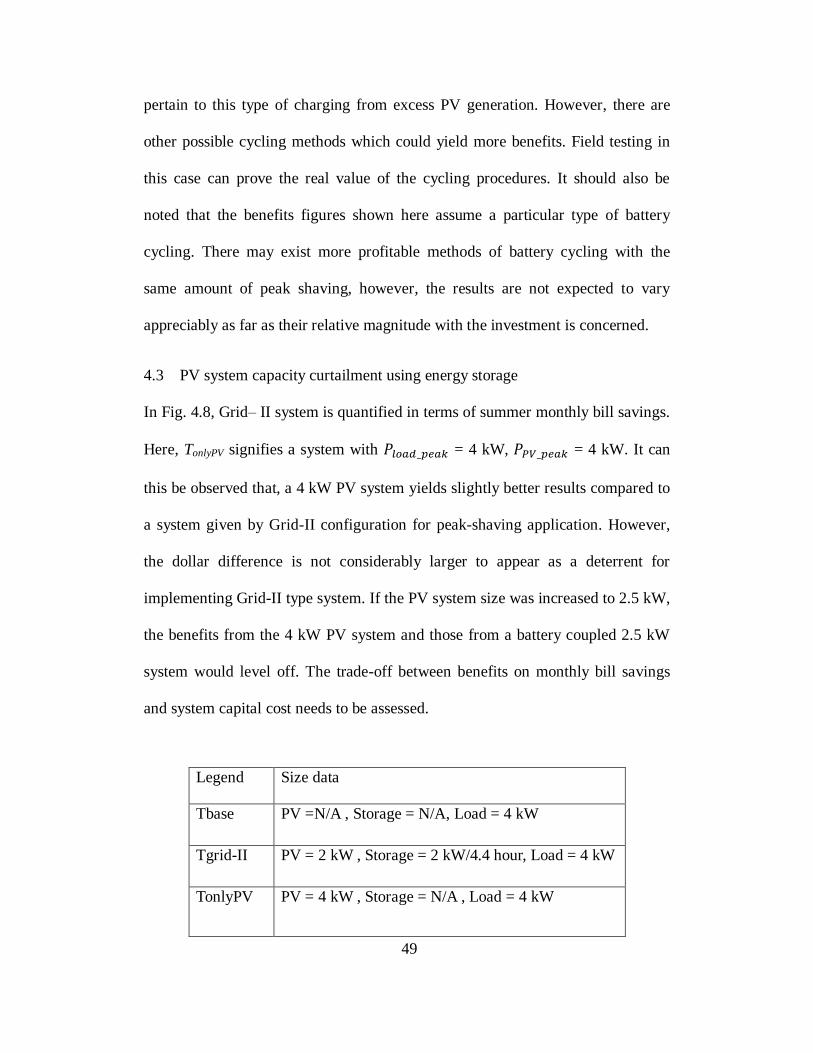
In Fig. 4.8, Grid– II system is quantified in terms of summer monthly bill savings.
Here, TonlyPV signifies a system with = 4 kW, = 4 kW. It can
this be observed that, a 4 kW PV system yields slightly better results compared to
a system given by Grid-II configuration for peak-shaving application. However,
the dollar difference is not considerably larger to appear as a deterrent for
implementing Grid-II type system. If the PV system size was increased to 2.5 kW,
the benefits from the 4 kW PV system and those from a battery coupled 2.5 kW
system would level off. The trade-off between benefits on monthly bill savings
and system capital cost needs to be assessed.
Legend Size data
Tbase PV =N/A , Storage = N/A, Load = 4 kW
Tgrid-II PV = 2 kW , Storage = 2 kW/4.4 hour, Load = 4 kW
TonlyPV PV = 4 kW , Storage = N/A , Load = 4 kW

50
Figure 4.8 Summer monthly electricity bill comparison with Grid – I system
At the end, it should be particularly noted that the scenarios considered here
assume that modification of demand profiles of customers due to energy storage
dispatch does not prompt a change in the tariff structure it refers to during the
course of storage system’s life-time. In other words, the tariff prices and their
behavior with respect to on-peak and off-peak hours are expected to remain the
same from year zero till the end of storage system life-time. With large
penetration of distributed storage catering to TOU energy management of every
individual customer, the overall demand profile of the network could be different
and the evening peak would shift to early morning hours when the battery owners
are expected to charge their storage. However, this analysis does not account for a
large penetration scenario and considers the cost-benefit with present tariff
structure.
4.4 An accelerated testing method for photovoltaic duty batteries
It is perceived that use of adequately sized batteries and a supporting tariff
structure would help reduce the rating of rooftop PV, thereby reducing the overall

51
system cost. This section proposes a simple low cost method to incorporate
accelerated laboratory testing of Lithium ion batteries to experimentally verify
their cycling behavior and dispatch of stored energy. The cycling strategy
discussed here is motivated by the fact that spring and summer in Arizona,
invariably see enough excess PV output in the morning which can be
conveniently stored and used to maximize on-peak energy savings thereby
completely eliminating the off-peak charging costs. The indoor system built for
the study is seen as a small scale replication of actual on-line system. With the
accelerated testing method described, it was possible to have the battery closely
follow the charging pattern from a PV source as in the field. Testing was
conducted with summer specific charge/discharge profiles on a prototype 73 Wh
Lithium ion battery. For storage dispatch, a typical residential load profile in
Arizona seen with Salt River Project (SRP) tariff plan E-26 was implemented
[10]. Also, ability of the system to recover from a low state of charge to full
charge following insufficient charging was analyzed.
The average summer PV output, customer demand corresponding to E-26 TOU
plan and battery profile corresponding to 40% peak shave target are shown in Fig.
4.9. The hourly retail electricity prices are also shown with bars. It can be
observed that peak PV output and peak demand are displaced in time and summer
PV output is in excess during the daytime for six hours atleast.
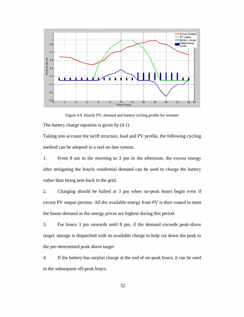
52
Figure 4.9 Hourly PV, demand and battery cycling profile for summer
The battery charge equation is given by (4.1)
Taking into account the tariff structure, load and PV profile, the following cycling
method can be adopted in a real on-line system.
1. From 8 am in the morning to 3 pm in the afternoon, the excess energy
after mitigating the hourly residential demand can be used to charge the battery
rather than being sent back to the grid.
2. Charging should be halted at 3 pm when on-peak hours begin even if
excess PV output persists. All the available energy from PV is then routed to meet
the house demand as the energy prices are highest during this period.
3. For hours 3 pm onwards until 8 pm, if the demand exceeds peak-shave
target, storage is dispatched with its available charge to help cut down the peak to
the pre-determined peak shave target
4. If the battery has surplus charge at the end of on-peak hours, it can be used
in the subsequent off-peak hours.
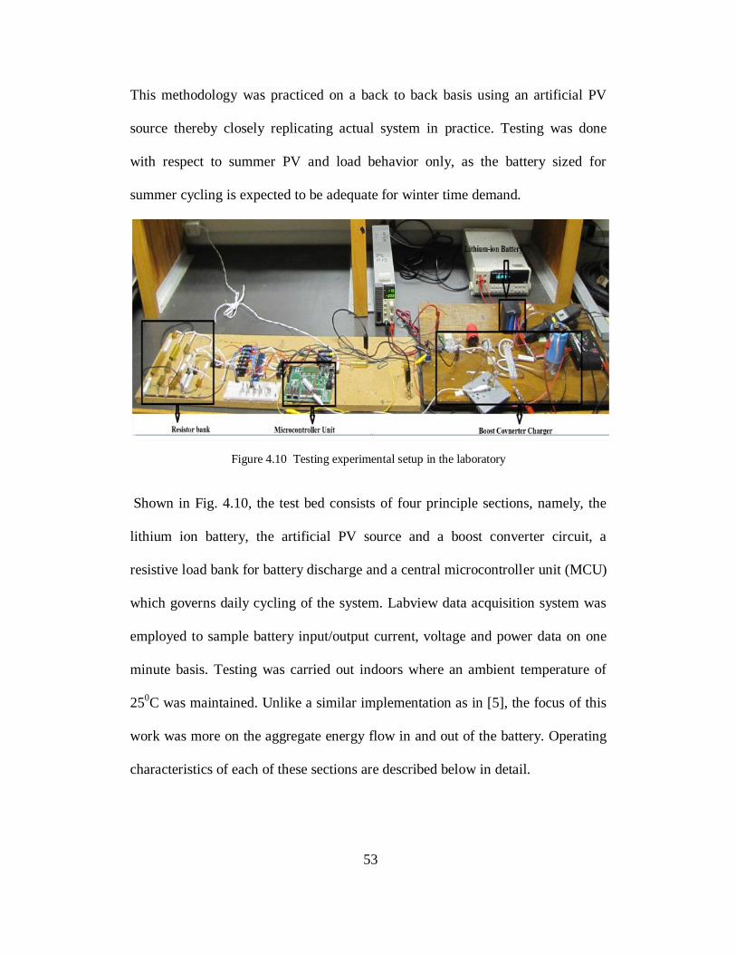
53
This methodology was practiced on a back to back basis using an artificial PV
source thereby closely replicating actual system in practice. Testing was done
with respect to summer PV and load behavior only, as the battery sized for
summer cycling is expected to be adequate for winter time demand.
Figure 4.10 Testing experimental setup in the laboratory
Shown in Fig. 4.10, the test bed consists of four principle sections, namely, the
lithium ion battery, the artificial PV source and a boost converter circuit, a
resistive load bank for battery discharge and a central microcontroller unit (MCU)
which governs daily cycling of the system. Labview data acquisition system was
employed to sample battery input/output current, voltage and power data on one
minute basis. Testing was carried out indoors where an ambient temperature of
250C was maintained. Unlike a similar implementation as in [5], the focus of this
work was more on the aggregate energy flow in and out of the battery. Operating
characteristics of each of these sections are described below in detail.
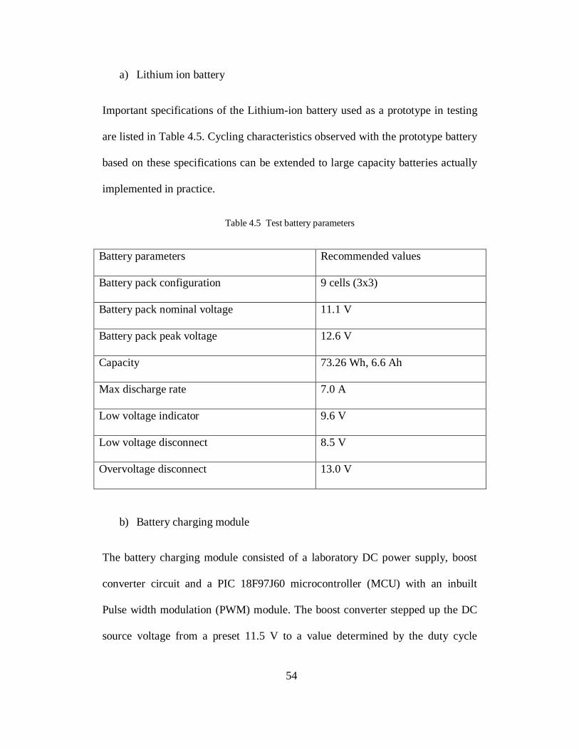
54
a) Lithium ion battery
Important specifications of the Lithium-ion battery used as a prototype in testing
are listed in Table 4.5. Cycling characteristics observed with the prototype battery
based on these specifications can be extended to large capacity batteries actually
implemented in practice.
Table 4.5 Test battery parameters
Battery parameters Recommended values
Battery pack configuration 9 cells (3x3)
Battery pack nominal voltage 11.1 V
Battery pack peak voltage 12.6 V
Capacity 73.26 Wh, 6.6 Ah
Max discharge rate 7.0 A
Low voltage indicator 9.6 V
Low voltage disconnect 8.5 V
Overvoltage disconnect 13.0 V
b) Battery charging module
The battery charging module consisted of a laboratory DC power supply, boost
converter circuit and a PIC 18F97J60 microcontroller (MCU) with an inbuilt
Pulse width modulation (PWM) module. The boost converter stepped up the DC
source voltage from a preset 11.5 V to a value determined by the duty cycle

55
programmed in MCU which controlled the charge flow into the battery terminals.
Steps implemented to determine power input to the battery are explained below.
1. With 11.5 V set at the boost converter input, battery current and power
input were calculated using (4.3, 4.4).
(4.3)
(4.4)
% (4.5)
Where, , , are battery charging current, voltage and power
respectively. is the instantaneous battery terminal voltage. indicates the
PWM duty cycle value while is the internal resistance of the battery in
ohms.
2. was limited to 1.7 A (0.25C) as per the manufacturer’s
recommended battery charging rate. Maximum charging output of the boost
converter and the maximum duty cycle were thus limited to about 20 W and 12%
respectively as determined by (4.3), (4.4) and (4.5). Each charging step was of 30
minutes.
3. The hourly demand followed an established pattern in every round-trip of
cycling similar to shown in Fig. 4.9. Also, per unit hourly PV output closely
follows the variations in hourly insolation given in Wh/m2. 2004 hourly summer

56
insolation data obtained from NREL’s National Solar Radiation Data Base
(NSRDB) was normalized to a base of 1000 Wh/m2 using (4.6). The charging
energy in per unit of peak was then obtained from (4.3). Duty cycle input
of PWM corresponding to is given in (4.7).
(4.6)
(4.7)
Where, S is the hourly solar irradiance in Wh/m2 and is 12% as from step 1,
is expressed in per unit .
4. With this configuration, it was possible to charge the battery with the
amount of watts in every charging step as dictated by the programmed duty
cycles. Any charging pattern could thus be reproduced if charging peak rating was
known.
For the boost converter circuit, a 200 uH inductor and 220 uF capacitor were
selected in order to have output current ripple within 10% and output voltage
ripple within 5% of their ratings. An EPHC – Smart DC voltage controller was
used to indicate if the battery level was full, the battery was being overcharged or
was completely discharged. The microcontroller PWM unit was programmed
using PICkit-3 and its frequency was set at 100 kHz.

57
c) Battery discharge module
The MCU switched between charge and discharge modes by operating a simple
relay, thereby making the system work continuously once put to operation. In
order to replicate a six step discharge (3 pm – 9 pm), a switching resistor bank
was constructed. The battery was allowed to discharge into the bank with the load
switched every 30 minutes. Each of the six legs of the resistor bank had a DC
relay with a 3V DC coil. They were operated in response to the signals from the
MCU register bits set as 0 or 1. Similar to the charging current, the maximum
discharge current supplied to the load was limited to 2.25 A (0.3 C). The
maximum possible power output of battery is given by (4.8).
(4.8)
Where, denotes the maximum output of the battery in Watts,
is the average discharge voltage (about 11.1 V) of the battery at
maximum discharge rate and is the maximum discharge current of
2.25 A. With different switching combinations of resistor bank, it was possible to
reproduce the discharge loadshape by switching appropriate branches. The system
was operated in Back to back charge and discharge modes following signals from
the MCU unit.
Fig. 4.11 depicts the reproduction of expected cycling profile for battery cycling
using the controlled DC voltage source and load bank. The right plot in Fig. 4.11
indicates the expected variation in cycling whereas the left plot suggests actual
cycling profile observed. It should be noted that in every 30 minute charging step,

58
the one minute power reading remained within 5% of its starting value. Positive
values in the figure indicate charging whereas negative values indicate
discharging of the battery. The cycling hours indicate total number of hours for
which one round-trip cycle lasts.
Figure 4.11 Comparison of reproduced and expected battery cycling profiles
d) Data acquisition system
NI-6025E (DAQ) with NI-SCXI-1000 power conditioner was used as the data
acquisition system to continuously record instantaneous battery current, voltage
and power. A Tektronix A622 AC/DC current probe was used to sense battery
current/voltage and provide them to the LabView DAQ. The data thus obtained
was processed in MATLAB to plot salient results.
With each round trip of battery cycling taking approximately six hours, one day of
testing provided four days’ data. Minute by minute data of battery terminal
voltage and current from each cycle were processed to determine the following
parameters
1. Average daily charge and discharge energies in Wh
2. Monthly charging and discharging energies in Wh

59
3. 30 minute average power intake and dispatch of the battery unit.
4. State of charge of the battery during its cycling
Figure 4.12 Average charging and discharging power observed in each step of cycling
Average charging Wh reading for a round-trip was about 45 Wh with the
programmed charging profile. 30 minute average power consumed and dispatched
by the battery during its cycling is shown in Fig. 4.12. Variations in the average
charging power in each step are reflective of the variability in the excess PV
power produced on hourly basis every day. The variability was due to
proportional real time irradiance parameter introduced in microcontroller duty
cycle control function. The first battery discharge began with the battery state of
charge at 100% resulting in higher dispatch. However, as the cycling progressed,
the peak dispatch settled to about 25 W as given by (4.8).

60
Figure 4.13 Daily Wh profile of battery cycling
Further, a 30 cycle test was performed to assess the ability of the battery to sustain
the 40 Wh daily load on an average.
Charging and discharging Wh for 20 days are shown in Fig. 4.13. It was seen that
inspite of considerable variability in PV charging of the battery, it was able to
supply about 40 Wh of energy on daily basis. Corresponding to day 16 and 17
cycling, due to insufficient charging of the battery, it was completely depleted
post its discharge. Enough charging in subsequent cycles ensured that the battery
regained its charge. Table 4.6 enlists some of the major performance parameters
observed during the month long cycling.

61
Table 4.6 Summary on monthly battery cycling performance
System performance parameters Summer (July)
Total 30 cycle Wh output 1210.7
Average Wh output per cycle 40.05
Average peak power output in W 25
Total 30 cycle Wh input 1470.5
Average Wh input per cycle 45.43
Maximum battery SOC (%) 92.5 (Cycle 3)
Minimum battery SOC (%) 20 (cycle 25,26)
Average battery SOC (%) 63.1
Key observations of this chapter
1. Size requirement for 40% peak-shaving was determined and
corresponding cost indices were calculated. The cost of adding an energy storage
component to the PV system was observed to be much larger in magnitude
compared to the value added in terms of benefits.
2. A 2kW/4.4 hour energy storage was however capable of reducing PV
system size from initial 4 kW by atleast 40% to maintain the benefits or savings
from peak-shaving achieved with the PV original system size.
3. A laboratory prototype of battery charging was helpful in understanding
the daily cycling of batteries in photovoltaic applications.

62
Chapter 5. SERVICE SPECIFIC COST-BENEFIT ANALYSIS OF BESS
5.1 Introduction
In the previous chapter, cycling of a domestic storage unit in peak-shaving
applications was studied using a 10.35 kWh battery model. In this chapter, the
same sized storage system is analyzed for its value in load-shifting, demand
charge management. Also, ability of distributed energy storage on the grid to
engage in substation peak-shaving is studied. ESVT 3- BETA presents a useful
tool to explicitly evaluate the economic value of battery energy storage in a
number of load management services. Battery Energy Storage Systems and the
services addressed in this study are listed in Table 5.1.
Table 5.1 Load management applications studied
Name of the service Perspective of Use (Utility or End-user)
Retail Time-of-Use (TOU) energy time-
shift
End-user
Retail demand charge management End-user
Distribution investment deferral Utility
For retail TOU time-shift and distribution investment deferral, value of the
storage system with and without associated PV generation has been assessed.
Retail demand charge management service however, considers only the storage
component. Storage system specifications are appropriately selected for each of
the services. Fig. 5.1 gives the service hierarchy which the ESVT – 3 Beta storage
dispatch algorithm follows within a set of different services.

63
Figure 5.1 Dispatch hierarchy map for ESVT – 3 Beta (Source ESVT – 3 Beta Manual)
5.2 Service – I: Retail TOU Energy Time-shift
a) Configuration – I : Storage-alone system
Introduction
The ensuing section determines economic value of operating customer premises
energy storage with a Time-of-Use tariff. Basis of operation here is buying energy
during off-peak hours to charge the storage and sell energy during on-peak hours
by dispatching the storage. As a result, every day, throughout the year, the battery
is charged after midnight during low retail price hours and discharged in the
evening when the customer demand peaks. This takes into account the tariff price
spread which is optimally utilized to maximize profits from the storage dispatch.
The case was modeled in ESVT 3- Beta.

64
Input indices
This configuration assumed the TOU tariff structures E-21 and E-26. Some of the
important system specifications are listed in Table 5.2. As mentioned, returns
from operating in this configuration are sensitive to the tariff structure price
spread and differential between on-peak and off-peak retail prices.
Table 5.2 Input parameters for the current case
Input index Specification
Peak house demand (Pload) (kW) a) 2
b) 3
Peak charge/discharge rate (Pbatt) (kW) a) 2
b) 3
Maximum battery capacity (kWh) 10.35
Depth of discharge of battery (DoD) (%) 80
Roundtrip efficiency (η) (%) 85
Energy storage subsystem cost ($/kWh) 900
Power conditioning subsystem cost ($/kW) 400
Battery replacement cost ($) 2000
Discount rate (%) 5.96
Annual energy price escalation rate (%) 3

65
Results
Net present value (NPV) of cost and benefit with the assumed discount rate is
shown in Table 5.3. NPV of cost takes into account battery and inverter
replacement costs also.
A representative summer day energy storage dispatch is shown in Fig. 5.1. It can
be observed that hours of discharge for E-21 tariff are three whereas for E-26
battery discharges for five hours. The net demand during the hours of storage
discharge is almost fully compensated. The net demand ( shape obtained
after energy storage dispatch can be simply given by (5.1) and (5.2). Here,
correspond to hourly customer demand and hourly battery
discharge in kW.
(5.1)
(5.2)
Figure 5.2 Summer hourly storage dispatch and net load for E-21 and E-26 customers
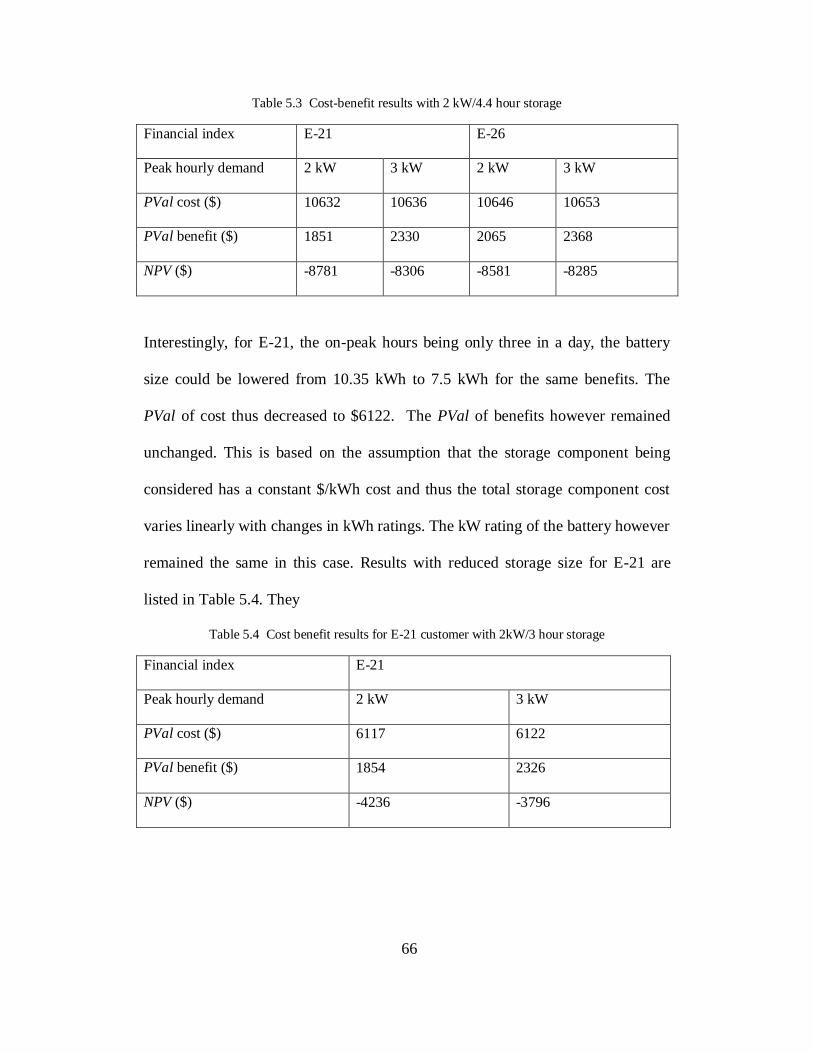
66
Table 5.3 Cost-benefit results with 2 kW/4.4 hour storage
Financial index E-21 E-26
Peak hourly demand 2 kW 3 kW 2 kW 3 kW
PVal cost ($) 10632 10636 10646 10653
PVal benefit ($) 1851 2330 2065 2368
NPV ($) -8781 -8306 -8581 -8285
Interestingly, for E-21, the on-peak hours being only three in a day, the battery
size could be lowered from 10.35 kWh to 7.5 kWh for the same benefits. The
PVal of cost thus decreased to $6122. The PVal of benefits however remained
unchanged. This is based on the assumption that the storage component being
considered has a constant $/kWh cost and thus the total storage component cost
varies linearly with changes in kWh ratings. The kW rating of the battery however
remained the same in this case. Results with reduced storage size for E-21 are
listed in Table 5.4. They
Table 5.4 Cost benefit results for E-21 customer with 2kW/3 hour storage
Financial index E-21
Peak hourly demand 2 kW 3 kW
PVal cost ($) 6117 6122
PVal benefit ($) 1854 2326
NPV ($) -4236 -3796

67
Results for monthly and annual benefits with respect to E-21 and E-26 tariffs for 2
kW and 3 kW peak evening loads are shown in Fig. 5.3 and Fig. 5.4 respectively.
These results again correspond to 2 kW/4.4 hour storage.
Figure 5.3 PVal of monthly savings for E-21 and E-26 tariffs
Figure 5.4 Annual savings for E-21 and E-26 tariffs with 2kW/4.4 hour storage

68
Key observations
For all configurations and sizes of storage studied, the life-cycle cost of storage
was observed to be much higher than the benefits earned. Cost of battery in
$/kWh was one of the major factors directly impacting the overall cost-effectively
of the system. On a comparison basis between E-21 and E-26 tariffs, there was no
appreciable difference in the annual revenue earned with 4.4 hour storage. For a 3
kW peak demand, returns from E-21 and E-26 were closely matched. With
respect to E-21 however, the differential in the annual earnings between 2 kW and
3 kW peak demands was noticeably higher than that for E-26. Also for E-21 the
battery size could be lowered on account of fewer on-peak hours compared to E-
26 thereby reducing the system cost and overall increased NPV.
b) Configuration - II : Battery assisted PV system
Introduction
Battery energy storage could be seen as a means to use an existing PV system
more efficiently and add value to it by practicing right battery cycling procedure.
The basis of formation of this case lies in that fact that peak PV output and peak
residential time-of-use prices are not coincident, resulting in less energy bill
savings than if the PV output occurred during the peak hours. During on-peak
periods, the storage is dispatched such that difference in the demand and PV
generation is supplied by it. In this section, a detailed value analysis of a storage
coupled PV system is carried out to estimate the value of a 10.35 kWh Lithium-

69
ion storage if operated in conjunction with suitably sized PV system. The peak PV
capacity of the system is varied from 2 kW to 5 kW to understand if value of
storage changes with PV system size. The costs and benefits presented in this case
exclusively model the storage component and exclude those of PV system.
Input indices
Table 5.5 enlists some of the major inputs defining the storage system modeled
for this case. The same OpenDSS PV system model was used to obtain hourly PV
generation. In ESVT 3- BETA, although a PV generation profile is selected, the
storage is charged only from the grid based on its perfect foresight assessment.
The battery discharge occurs during on-peak hours everyday and also during
certain off-peak hours if the battery has sufficient capacity left and if subsequent
hours are expected to produce enough PV output. ESVT 3- BETA’s algorithm
looks for opportunities where the difference in prices between hours within a day
can support a profitable time-shifting opportunity, after accounting for losses, and
decides the best charging and discharging hours for storage to maximize savings.

70
Table 5.5 Input battery and load parameter specifications
Input index Specification
Peak house demand (Pload) (kW) a) 2
b) 3
Peak charge/discharge rate (Pbatt) (kW) 2
Maximum battery capacity (kWh) 10.35
Depth of discharge of battery (DoD) (%) 80
Roundtrip efficiency (η) (%) 85
Energy storage subsystem cost ($/kWh) 900
Power conditioning subsystem cost ($/kW) 400
Battery replacement cost ($) 2000
Discount rate (%) 5.96
Annual energy price escalation rate (%) 3
Results
Fig. 5.5 shows a representative summer day energy storage dispatch along with
hourly PV generation and net load for E-21 and E-26 tariffs.
(5.3)
(5.4)

71
Figure: 5.5 Summer Net load profile for E-21(Left) and E-26(Right)
It can be observed that the summer hourly demand is fully compensated during
daytime with PV. Storage discharge begins with on-peak hours and continues into
subsequent off-peak hours if sufficient charge is left. Identical pattern in the net
load is observed for both E-21 and E-26.
Table 5.6 and Table 5.7 list some of the principle financial parameters of the
system with respect to the assumed PV and demand ratings. It should be noted
that the benefits shown here are exclusive of savings from PV generation. These
benefits amount from cycling the storage only. The overall savings from a system
consisting of PV and storage can be obtained by adding savings earned from PV
to those obtained here. However, the results shown are indicative of the value
addition to the system by having a PV source charging the storage.
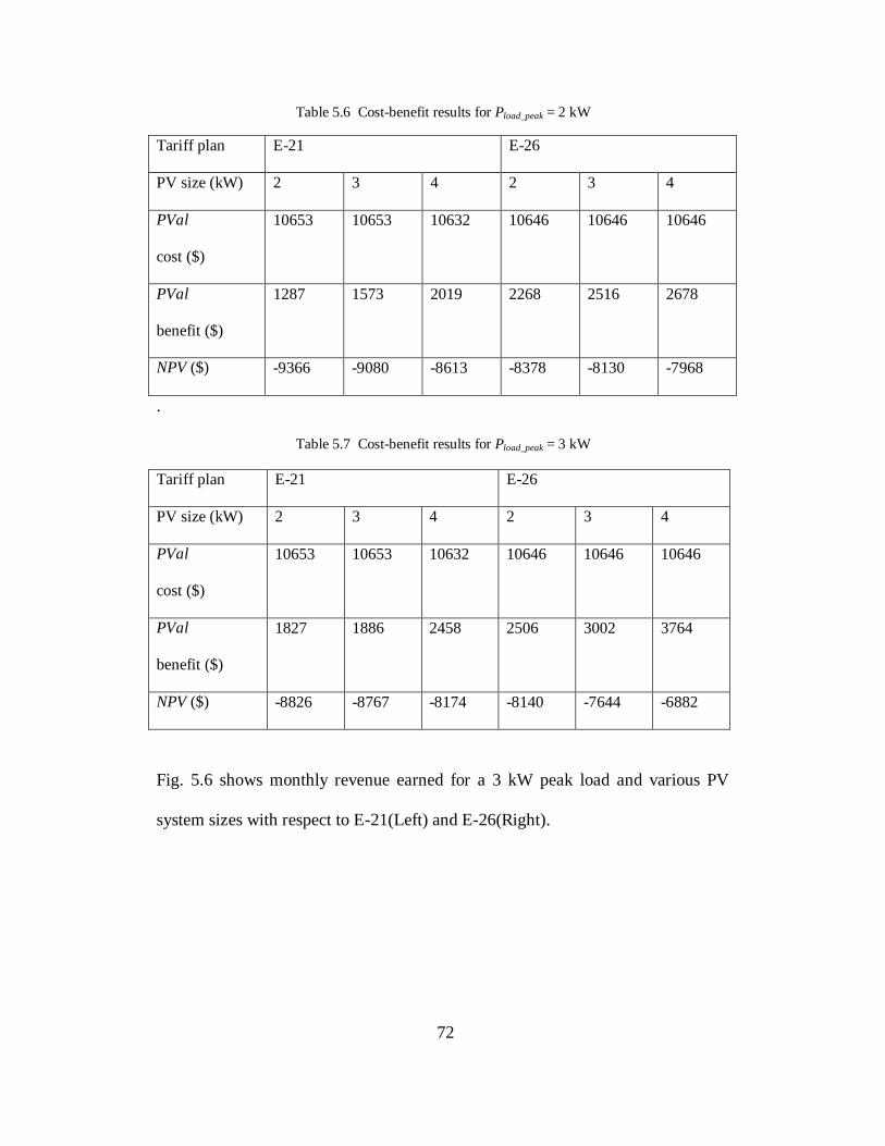
72
Table 5.6 Cost-benefit results for Pload_peak = 2 kW
Tariff plan E-21 E-26
PV size (kW) 2 3 4 2 3 4
PVal
cost ($)
10653 10653 10632 10646 10646 10646
PVal
benefit ($)
1287 1573 2019 2268 2516 2678
NPV ($) -9366 -9080 -8613 -8378 -8130 -7968
.
Table 5.7 Cost-benefit results for Pload_peak = 3 kW
Tariff plan E-21 E-26
PV size (kW) 2 3 4 2 3 4
PVal
cost ($)
10653 10653 10632 10646 10646 10646
PVal
benefit ($)
1827 1886 2458 2506 3002 3764
NPV ($) -8826 -8767 -8174 -8140 -7644 -6882
Fig. 5.6 shows monthly revenue earned for a 3 kW peak load and various PV
system sizes with respect to E-21(Left) and E-26(Right).

73
Figure 5.6 Monthly benefits for 3 kW peak load with E-21(Left) and E-26(Right) tariffs
Fig. 5.7 shows a comparison of annual savings from storage cycling for Pload = 2
kW and Pload = 3 kW with various PV sizes as applicable to E-21 and E-26 tariffs.
The left plot shows NPV of benefits for E-21 tariff whereas the right plot shows
NPV of benefits for E-26.
Figure 5.7 Annual revenue for E-21(Left) and E-26(Right) tariffs with different PV sizes
To understand the difference in energy storage dispatch in presence of PV, hourly
assessment of tariff price spread, customer demand profile and number of on-

74
peak, off-peak hours is necessary. Fig. 5.8 shows hourly revenue earned from
storage on a summer day with both E-21 and E-26 tariffs.
Figure 5.8 E-21 and E-26 storage dispatch and hourly retail pricing
Key observations
The results in this case were obtained with ESVT 3-Beta, Although a positive
relationship was observed between photovoltaic array size with respect to load
size, it was observed that the cost of storage was significantly more in all cases
than the present value of annual revenue earned from cycling the storage. Benefits
and costs were attributed to storage system only and were compared with respect
to one another. PV costs and benefits were not included. . This meant that,
addition of a storage system of about 10 kWh to an existing PV system for
providing the single service of retail time-of-use energy time-shifting was not
observed to be cost-effective at current costs. Installed cost of storage needs to
fall below $200/kWh to make this a cost-effective case.

75
The benefits nevertheless presented a comparison basis for tariffs E-21 and E-26
in terms of the returns they yield over a 20 years period. Returns from E-26 were
found to be about 50% higher than those from E-21 for the same size of system.
The reason was that, the on-peak hours for E-21 tariff which are 3 pm to 6 pm,
coincide with considerable PV output period. As a result the on-peak storage
discharge is limited and it was pushed further into the off-peak periods. In
comparison, on- peak hours of E-26 last for about 3 hours after the sun sets,
allowing storage to discharge more during on-peak period. Accumulated returns
are therefore more for E-26 tariff. Increasing the PV size beyond demand peak
pushes bulk of the storage discharge more towards the evening hours.
5.3 Service – II: Retail Demand Charge Management
Introduction
Unlike residential retail electricity charge which is based solely on kWh of energy
consumed, demand charge is applied based on the peak instantaneous (usually 15
min average) kW of power demanded by a customer over the course of a month.
Industrial or commercial customers, which often have large capacity electrical
machines such as water pumps, motors, or compressors, often have tariffs which
include a demand charge. E-36 and E-32 tariff plans of SRP consist of the
demand charge rider and are applicable to commercial units. The focus of this
case is to estimate savings to a customer under E-36 and E-32 tariff from storage
dispatch as a means to mitigate the demand charges. kWh based charge for E-36
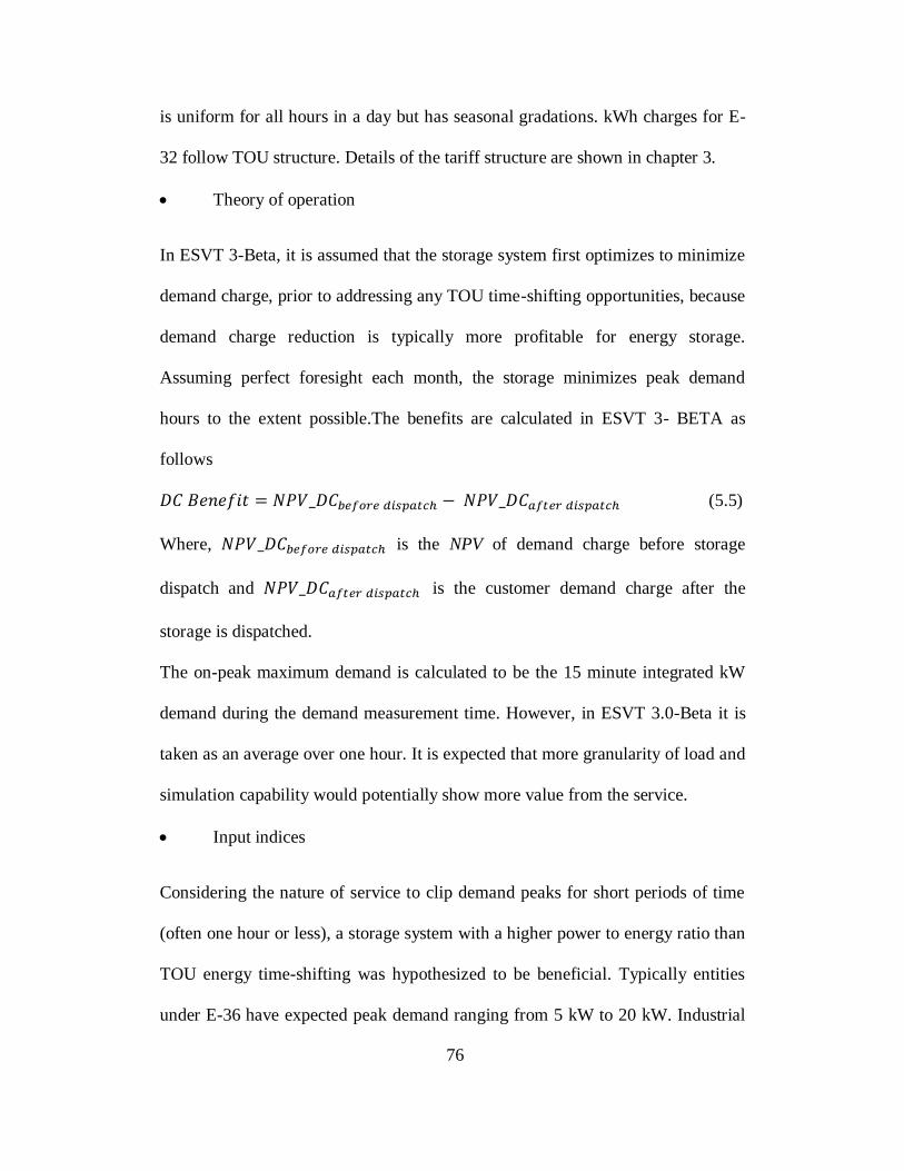
76
is uniform for all hours in a day but has seasonal gradations. kWh charges for E-
32 follow TOU structure. Details of the tariff structure are shown in chapter 3.
Theory of operation
In ESVT 3-Beta, it is assumed that the storage system first optimizes to minimize
demand charge, prior to addressing any TOU time-shifting opportunities, because
demand charge reduction is typically more profitable for energy storage.
Assuming perfect foresight each month, the storage minimizes peak demand
hours to the extent possible.The benefits are calculated in ESVT 3- BETA as
follows
(5.5)
Where, is the NPV of demand charge before storage
dispatch and is the customer demand charge after the
storage is dispatched.
The on-peak maximum demand is calculated to be the 15 minute integrated kW
demand during the demand measurement time. However, in ESVT 3.0-Beta it is
taken as an average over one hour. It is expected that more granularity of load and
simulation capability would potentially show more value from the service.
Input indices
Considering the nature of service to clip demand peaks for short periods of time
(often one hour or less), a storage system with a higher power to energy ratio than
TOU energy time-shifting was hypothesized to be beneficial. Typically entities
under E-36 have expected peak demand ranging from 5 kW to 20 kW. Industrial

77
loads could have their peak demand well above 50 kW. However, for the purpose
of this study, to better match the 2 kW, 10.35 kWh energy storage system, a
scaled down nominal 7 kW peak load was considered. The size of storage was
then increased to see if it significantly affected the returns.
Table 5.8 Input indices for demand charge management service
Input index Specification
Peak demand (kW) 1. 7
2. 10
3. 20
Peak charge/discharge rate of storage (kW) 2
Maximum battery capacity (kWh) 10.35
Depth of discharge of battery (%) (DoD) 80
Roundtrip efficiency (%) (η) 85
Energy storage subsystem cost ($/kWh) 900
Power conditioning subsystem cost ($/kW) 400
Battery replacement cost ($) 2000
Discount rate (%) 5.95
Demand charge escalation (%) 4
Fig. 5.9 shows annual and summer daily hourly load profile for E-36 and E-32
tariffs. The summer daily load profile indicates that the demand peaks at around
12 PM and remains within 10% margin till 9 PM.

78
Figure 5.9 8760 load profile for E-36 and E-32 tariffs
Results
E-36 tariff does not have a TOU structure. As a result, cycling of storage results
in losses as the battery charging costs turn out to be more than the battery
discharging costs on kWh basis. This occurs as the round-trip efficiency of the
storage is about 85% resulting in 15% losses in one round trip. Therefore, the
benefits associated with demand charge reduction will be offset somewhat by the
cost of charging efficiency losses. In contrast, E-32 tariff does have TOU energy
prices in addition to a demand charge. Comparison between the cost benefit
economics from each of the tariffs is shown in Table 5.9.
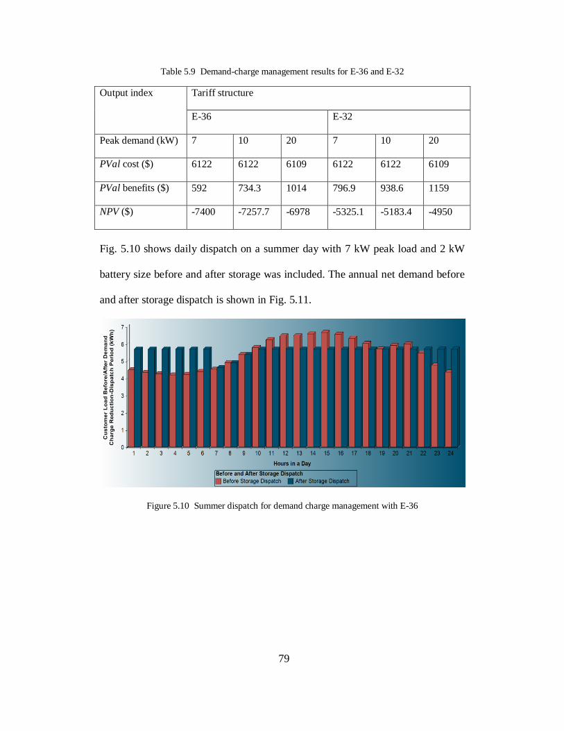
79
Table 5.9 Demand-charge management results for E-36 and E-32
Output index Tariff structure
E-36 E-32
Peak demand (kW) 7 10 20 7 10 20
PVal cost ($) 6122 6122 6109 6122 6122 6109
PVal benefits ($) 592 734.3 1014 796.9 938.6 1159
NPV ($) -7400 -7257.7 -6978 -5325.1 -5183.4 -4950
Fig. 5.10 shows daily dispatch on a summer day with 7 kW peak load and 2 kW
battery size before and after storage was included. The annual net demand before
and after storage dispatch is shown in Fig. 5.11.
Figure 5.10 Summer dispatch for demand charge management with E-36

80
Figure 5.11 Net demand with demand charge management before and after storage dispatch
Key observations
The input load data used for this service was in hourly form and does not
comprehensively represent the type of data that would be desirable to study
demand charge management. The data was typical and averaged by hour. An
actual load data is expected to depict demand spikes on certain hours or certain
days which the demand charge management service is intended to address.
It can be observed that the benefits earned by the system from reducing the
demand charge are reduced due to losses in charging capacity as the E-36 kWh
tariff pricing is flat. Benefits were higher for E-32 tariff as TOU charges applied.
Increasing the peak load also showed some improvement in the returns earned,
although the cost of storage remained much more than the benefits.
0
1
2
3
4
5
6
7
8
1 33
8
675
10
12
1349
16
86
2023
23
60
2697
30
34
3371
37
08
4045
43
82
4719
50
56
5393
57
30
6067
64
04
6741
70
78
7415
77
52
8089
84
26
De
man
d in
kW
Annual 8760 dispatch 7 kW peak demand and 2kW/4.4 battery
Before Dispatch
After Dispatch

81
Based on the simulation and value calculations in ESVT 3-Beta, benefits from
demand charge alone may not be able to justify the investment in storage. The
same storage system could be used for other services such as reliability and power
quality to increase the value. If used for reliability, a certain quantity of storage
can be reserved as back-up and the remaining capacity can be used for mitigating
demand-charges, or the reliability value will be calculated by virtue of the energy
available in the battery without affecting its operation, because the battery still
contains energy for a significant duration of its life. Such synergies need to be
assessed based on storage size.
Note: The behavior of energy storage dispatch with increase in battery discharge
rate (kW) is being investigated by EPRI. The ESVT version used here was beta.
5.4 Service – III: Distribution Investment Deferral
Introduction
For this grid service, the customer premise sited residential storage, ‘Edge of
Grid’ energy storage (sometimes referred to as Community Energy Storage) as
well as bulk storage near the substations are assessed in terms of their
effectiveness to delay investments in distribution system upgrade. Due to
economic recession in the recent past, the yearly load growth in Arizona has been
negligible or even negative. However, continued higher summer peak
temperatures above 110 0F have been a cause of increased demand during
afternoon hours. With improvement in the economic environment, the load
growth is expected to pick up in the next decade. Also, this type of service is

82
highly site-specific. In some cases even when the average annual load seen at the
substation is expected to fall, certain distribution transformers might see an
increased demand due to local development. Energy storage can provide a viable
alternative to lower or maintain the same summer peak load and delay bulky
investments in upgrading the substation or feeder equipment.
Theory of operation
In ESVT 3-Beta, deferral benefits are calculated in terms of the ability of energy
storage on the grid to shave the distribution substation transformer peak by a
required % of base year load peak. In other words, the benefit is given as the NPV
of investments deferred by the number of years of deferral. The deferral years are
determined to be equal to the period for which the storage is able to keep the
annual peak below the preset percentage. Annual investments made on system
upgrade by utility, annual demand profile and annual load growth are the three
primary inputs for this calculation. The annual load-shape and annual peak seen at
the substation transformer is obtained from actual SRP residential feeder data
modeled in OpenDSS. Load target is defined such that the storage dispatch tries to
meet only that percentage of the base load.
The energy storage modeled for this service could be an aggregate of distributed
storage devices on the grid or it can be modeled as bulk energy storage located
near the substation. While the bulk energy storage is assumed to be owned and
controlled by the utility, dispatch and control of distributed energy storage
whether community or customer premises type, can be modeled as utility
controlled as well as end-user controlled.

83
Input indices
The demand profile seen at the point of interest or in this case a substation is the
net demand of a number of smaller loads across the network downstream of the
substation. As a result, a distribution feeder stemming from a substation even if
predominantly residential, the substation as a whole could be serving a number of
industrial and commercial establishments whose demand for electricity follows a
much different profile than a residential neighborhood does. The net demand
shape seen at the substation transformer hence can possibly be quite different
from that observed at the head of a feeder serving residential loads. Also,
presence of other distributed generation on the network such as PV further alters
substation load profile. In ESVT – 3 Beta, for this service, the energy storage is
assumed to cater to the net demand profile at the point of interest when all
distributed generation is included. Further analysis is divided in two sub-
categories, one considering distributed PV generation on the grid while the second
neglects any PV or distributed generation penetration. Some of the input indices
common to all sub-cases are given in Table 5.10. It should be noted that when the
storage is dispatched to maintain annual peak to its Year 0 level, it is paid the
market price (Palo Verde) for providing electricity and charged the same hourly
market price when it is being charged during off-peak hours. The benefits include
these benefits on account of electricity sale. The 8760 market prices at Palo Verde
are given in Fig. 5.12.

84
Figure 5.12 Hourly market price of electricity at Palo Verde (2011)
Table 5.10 Input indices for distribution investment deferral service
Input index Specification
Distribution load growth rate (%) a) 0.5
b) 1
c) 2
One-time distribution investment ($) 4,000,000
Distribution investment period (years) 30-40
Storage maximum discharge rate (MW) a) 0.5
b) 1
Storage discharge hours 4
Capital cost of storage ($/kWh) 600
Capital cost of storage ($/kW) 400

85
OpenDSS Model of SRP feeder
In order to determine the substation load profile as input to ESVT – 3 Beta, an
SRP feeder was modeled in OpenDSS with and without distributed PV generation
[37]. The distribution substation considered gives rise to five radial feeders of
which one was modeled in explicit detail and an aggregated load profile for the
other four feeders was considered. Resultant load profile seen at the substation
and also at the head of feeder modeled in detail was obtained. Table 5.9
summarizes the details of the OpenDSS feeder model. A MATLAB program was
developed and operated via the COM interface of OpenDSS to study the response
of various feeder parameters in presence of distributed energy storage and PV.
Table 5.11 Description of OpenDSS model of SRP residential feeder
Feeder parameters Specifications
Name MC114
kV 12.47
Circuit miles 13.12
Number of feeders on the same substation 5
Number of customers on the feeder modeled 1497
Customer class Suburban, mainly residential
Load factor (%) 50
Capacitors 1200 kVAR x 3
Lines Mostly underground
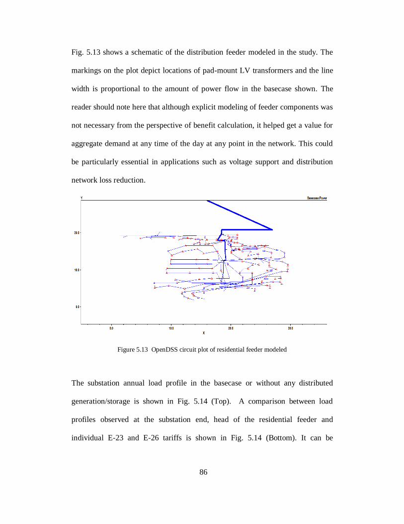
86
Fig. 5.13 shows a schematic of the distribution feeder modeled in the study. The
markings on the plot depict locations of pad-mount LV transformers and the line
width is proportional to the amount of power flow in the basecase shown. The
reader should note here that although explicit modeling of feeder components was
not necessary from the perspective of benefit calculation, it helped get a value for
aggregate demand at any time of the day at any point in the network. This could
be particularly essential in applications such as voltage support and distribution
network loss reduction.
Figure 5.13 OpenDSS circuit plot of residential feeder modeled
The substation annual load profile in the basecase or without any distributed
generation/storage is shown in Fig. 5.14 (Top). A comparison between load
profiles observed at the substation end, head of the residential feeder and
individual E-23 and E-26 tariffs is shown in Fig. 5.14 (Bottom). It can be

87
observed that the substation demand peak occurs atleast two to three hours prior
to the occurrence of residential feeder peak during summer.
Figure 5.14 Annual and summer daily substation load
Results
Number of years for which the annual distribution investment is deferred through
this service in response to the annual substation load growth assumption was
assessed. Also the dispatch hours of grid energy storage and the number of
dispatch days were analyzed and compared. Substation demand profile and an
individual residential feeder demand profile were analyzed to understand the
energy storage discharge pattern. Variation in this pattern with additional
distributed PV penetration was analyzed, if any. Results for substation investment
deferral with 0.5 MW and 1 MW grid energy storage are shown in Table 5.12.

88
Table 5.12 Results for distribution investment deferral at substation
Service index Specification
Substation peak
(MW)
14.9
Residential feeder
peak (MW)
5.64
Annual load growth (%)
0.5 1 2
Storage size (MW) 0.5 1 0.5 1 0.5 1
Deferred years 6 13 3 6 1 3
Number of dispatch
days
11 22 11 22 11 22
PVal cost (Million$)
*
1.562 3.124 1.562 3.124 2.518 3.124
PVal benefits
(Million $)
0.981 1.712 0.54 0.981 0.37 0.54
Annual revenue from
deferral (Million
$/year)
0.193
* applicable to Utility owned storage
Fig. 5.15 shows how the net loads at the substation and on the residential feeder
was maintained at their respective base-case peak loads (2% annual load growth)

89
when an effective of 1 MW of storage was installed. Two representative summer
days were selected to depict the energy storage dispatch as obtained from ESVT –
3 Beta.
Figure 5.15 Substation (Top) and residential feeder head (Bottom) demand before and after
storage dispatch
Fig. 5.16 shows the number of dispatch days and battery state of charge during
year 3 of 1 MW/4.4 hour storage dispatch with 2% load growth assumed.

90
Figure 5.16 Battery SoC and number of dispatch days in year 3
Table 5.13 tabulates the results of distribution investment deferral service with
1MW, 4hour storage and an assumed annual load growth of 2%. The energy
storage was able to defer the substation investment by three years.
Table 5.13 Investment deferral results for 1MW, 4hour storage, 2% load growth in year 3
Investment deferral index (Day 225) Result
Annual peak load before dispatch (MW) 15.47
Annual peak load after dispatch (MW) 14.9
Number of deferral days 22
Number of days with more than 40% storage
depth of discharge
9
Substation load factor before dispatch (%) 51.49
Substation load factor after dispatch (%) 54.62

91
In this analysis pertaining to the use of energy storage only for distribution
investment deferral, it is assumed that the discharge of individual storage units on
the grid occurs during the substation peak hours. This may not be in the best
possible interest of the end-user who owns the storage unit, as the residential
demand peak and substation peak might differ in their occurrence. As a result, it
would be interesting to compare benefits to the end user if they follow the utility
peak and follow the local peak. Fig. 5.17 compares discharge specific to
distribution investment deferral to that for retail TOU service (E-21 and E-26).
Customer premises dispatch was modeled with scaled down substation load
profile as used in the deferral case.
Figure 5.17 Storage dispatch comparison between services I and III
Fig. 5.17 shows resultant substation demand before and after storage dispatch
when distributed PV generation is added to the basecase. Again the storage size
considered was 1 MW/ 4 hours with 2% annual load growth. Comparison with

92
the basecase results of the same configuration is also shown. The storage
discharge was seen to be following the same pattern in both cases, the magnitude
of discharge however was scaled proportionately. The added PV generation
modeled in OpenDSS was specified as follows.
PV modeling indices Specifications
Total number added PV installations on the
network
896
Peak rating of each PV installation (kW) 2
Total peak rating of distributed PV on the grid
(MW)
1.8 MW
Figure 5.18 Net substation demand profile before and after storage dispatch
Key observations
If the storage system was owned by a utility for deferring capacity upgrade
investments, the capital cost to own a Lithium-ion distributed storage facility was

93
found to be more than the avoided costs of system upgrade considering that it is
used only for investment deferral. However, as seen from the results, with storage
dispatch occurring only for a handful of days the system would remain idle for
most of the year. Practically, the same system can be used to provide a number of
other ancillary services such as spinning reserve support, frequency regulation,
power quality and reliability improvement and also as a means for energy
arbitrage. On the other hand, if storage on the grid was in the distributed form of
residential storage owned by individual end-users, no utility investment is
required and with proper control and automation infrastructure on the grid, their
collective effect in distribution investment deferral can be realized at the
substation.
5.5 Service – IV: Spinning Reserve Support and Energy Arbitrage
Battery energy storage can be dispatched as a spinning reserve resource due to its
high ramping rate. However, viability of this service is highly location and
requirement specific. In this section, value of battery energy storage is assessed
for SRP system with respect to spinning reserve support services. SRP does not
come under a deregulated or competitive electricity market structure.
SRP’s spinning reserve policies and practices
a) WECC standard BAL-STD-002-0- Operating Reserves states “The
combined unit ramp rate of each Balancing Authority's on-line, unloaded
generating capacity must be capable of responding to the Spinning Reserve
requirement of that Balancing Authority within ten minutes.”

94
b) NERC glossary terms it as “Unloaded generation that is synchronized and
ready to serve additional demand.”
c) At present, WECC does not account for energy storage as a spinning
reserve support option; however there are efforts in that direction as indicated in
the PNNL report
d) Distributed BESS, if used as spinning reserve resource, needs to be under
SRP’s control every hour. For substation sited BESS, spinning reserve
requirement and other services’ dispatch may overlap during on-peak hours
e) The hourly price for holding unloaded, online spinning reserve is in the
range of $5-10/MW, if the reserves were called for, its cost to SRP is close to
market price at Palo Verde, as shown in Fig.5.19.
f) Balancing Areas (BAs) have 105 minutes to reestablish lost reserve
capacity. SRP needs to carry 100-150 MW of spinning reserve every hour.
g) SRP has hardly bought reserve support from resources, other than its own
unloaded generators during the past 2 years.
h) Number of instances in 2012 when spinning reserve support was called for
was 516.

95
Figure 5.19 Hourly value for holding spinning reserve capacity to SRP
Keeping generators unloaded, costs SRP in the following ways
1. Start up cost and shut down costs
2. Generator ware and tear
3. Maintenance costs
4. Missed opportunities as generating resource
These cost constraints could be included as a part of a DC optimal power flow
program along with energy storage constraints on size and dispatch rates to assess
the additional cost savings to SRP on account of the factors mentioned above.
Service inputs
a) Price data – It is the hourly price in $/MW paid to the spinning reserve
resource to maintain the reserve. It is shown in Fig. 5.19.
b) Probability to dispatch – This is the probability that during a provision of a
synchronous reserve bid, the storage is actually required to discharge. In other
works, it is the percentage of the total number of hours the spinning reserve is

96
paid, for being available. Approximate value can be determined from experience
or analysis of contingencies and reliability indices. In this case a probability of
0.3% (25-30 events) is considered based on a reasonable judgment as real data
was unavailable.
Dispatch results
Here, relative benefits from three services are shown, namely spinning reserve
support and distribution investment deferral. The two services are independent of
each other and based on the hierarchy structure shown in Fig. 5.1. Dispatch days
for spinning reserve support have been determined from a Monte Carlo algorithm
within ESVT 3.0 (Beta). Results are shown in Table 5.14. Some of the key inputs
are mentioned below.
a) Plant life : 15 years
b) Storage size : 1 MW/4.4 hour
c) Distribution investment deferral : 2% load growth, 4 M one-time
investment
d) Spinning reserve support : 0.3% Probability to dispatch (25-30 events)
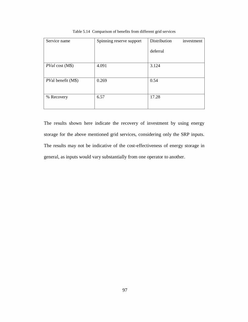
97
Table 5.14 Comparison of benefits from different grid services
Service name Spinning reserve support Distribution investment
deferral
PVal cost (M$) 4.091 3.124
PVal benefit (M$) 0.269 0.54
% Recovery 6.57 17.28
The results shown here indicate the recovery of investment by using energy
storage for the above mentioned grid services, considering only the SRP inputs.
The results may not be indicative of the cost-effectiveness of energy storage in
general, as inputs would vary substantially from one operator to another.

98
Chapter 6. CONCLUSION AND SCOPE FOR FUTURE RESEARCH
As the study has culminated into a service specific cost-benefit analysis, it
becomes imperative to bring out key inferences and conclusions by addressing
those particular services provided by BESS. They are mentioned below.
Conclusion
a) 40% domestic peak shaving
In this service, the excess rooftop PV (2-4 kW) energy generated during off-peak
hours was used to charge a 2kW/4.4 hour Lithium-ion battery and the same
battery with available SoC was discharged during on-peak hours. Earning from
this type of energy arbitrage aimed at achieving a 40% peak-shave target showed
about 30% increase in annual electricity bill savings with a 3.6 kW PV size.
However, the increase in savings was not observed to be commensurate with the
increase in life-time investment into the system due to the added battery
component. From a hardware approach, an indoor, accelerated battery charging
method developed demonstrated the cycling of batteries with duties similar to
those in photovoltaic applications. It gave a useful insight into battery round-trip
efficiencies and its ability to recover from a low SoC.
b) Retail TOU energy time shift
On an average, about 20% of the life-time investment in energy storage was
recovered in this service with various size assumptions for PV system, battery and
load. Results with E-21 and E-26 did not show an appreciable difference in the
annual revenue earned for 2kW/4.4 hour storage. It was however noticed that
battery hours of discharge for E-21 could be lowered to 3 and yet have the same

99
revenue. By addition of PV component, the storage discharge was pushed more
into late evening hours, which was useful in case of E-26 but it decreased the
value from storage in case of E-21.
c) Demand charge management
Demand charge management revenue was only about 10% of the life-time
investment in storage for the kind of demand profile assumed. This service can be
coupled to other customer premises services to serve as a value addition. Returns
from this service were observed to be sensitive to the nature of load and battery
discharge rate to some extent.
d) Distribution investment deferral
A 1 MW/4 hour Lithium-ion energy storage was assessed to defer investment into
an SRP distribution substation upgrade ($ 4M) by three years. This service
recovered about 17% of the life-time cost of energy storage. However, number of
days of dispatch for investment deferral was only about 15-20 during a year. This
would ensure that the storage could be used for other services such as ancillary
support, reliability during the remaining period when storage is idle.
e) Spinning reserve support
This service was assessed with the limited data that was available and by making
necessary approximations. In SRP’s case, stationary energy storage could be used
as spinning reserve support as a marginal requirement in place of unloaded
generators. The returns from 1 MW/4 hour energy storage as spinning reserve
support yielded about 5-10% of investment assuming 25-30 events of dispatch.

100
ESVT 3.0 (Beta) used for value analysis of energy storage in all the above
mentioned services was a useful tool to exclusively assess storage dispatch and
resulting benefit streams. The study also proved to be helpful to EPRI to further
understand the software and learn from the difficulties arising in the evaluation
process.
Scope for future research
The following aspects of BESS need to be addressed in detail in future
research
a) Focused market framework to include BESS in grid services
b) The third party aggregation benefits to the utility in terms of
distribution loss reduction, dispatch flexibility, demand response need
to be addressed in detail. They have a potential to substantially add to
the value of energy storage in distribution grid applications.
c) Better analysis tools with broader capabilities to assess BESS projects
with regards to their cost benefit analysis and the grid impact
d) Sustainable incentive structure to make BESS a viable business
proposal for both, manufacturers and customers at the residential level
e) Contribution of variation in grid parameters on the cost assessment i.e
a system perspective
f) Representation of economic, sizing and other system constraints in
greater detail in the storage dispatch optimization algorithms
g) Documentation and benchmarking of field-results

101
REFERENCES
[1] Department of Energy. (2012). DOE Energy Storage Database (beta).
Retrieved from http://www.energystorageexchange.org/
[2] Wang, U. (2011). The World’s Largest Lithium-Ion Battery Farm Comes
Online. Forbes. GreenTech. Retrieved from
http://www.forbes.com/sites/uciliawang/2011/10/27/worlds-largest-lithium-ion-
battery-farm/
[3] ABB. (2011). ABB LV Power Converter Solutions PCS100 ESS , 100 kVA to
20 MVA Energy Storage System Service and support. Product Brochure.
Retrieved from www.abb.com/powerelectronics
[4] Solar City, How solar power works. Retrieved from
http://www.solarcity.com/residential/how-solar-works.aspx
[5] Nicholas W. Miller, Robert S. Zrebiec, Robert W. Delmerico', George Hunt,
“Battery Energy Storage Systems for Electric Utility Industrial and Commercial
Applications,” Battery Conference on Applications and Advances, pp. 235-240,
9-12 Jan 1996.
[6] Panasonic. (2007). Meeting the Needs of Portable Electronic Devices,
product note.
[7] Nelson, P. A., Santini, D. J., Barnes, J.,” Factors Determining the
Manufacturing Costs of Lithium- Ion Batteries for PHEVs,” Electric Vehicle
Symposium - 24, pp. 1-12, 2009.
[8] S. Chhaya, “Large-Format Lithium-Ion Battery Costs Analysis,” Technical
update (Electric Power Research Institute), 1019923, 2010.
[9] D. Rastler, “Electricity energy storage technology options,” Technical update
1020676, EPRI, Dec 2010.
[10] Susan Schoenung; “Energy storage system cost update,” Sandia National
Laboratories, SAND2011-2730, April 2011.
[11] Narula, C., Martinez, R., Onar, O., Starke, M., & Andrews, G. (2011). Final
Report Economic Analysis of Deploying Used Batteries in Power Systems,
(June).Retrieved from
http://www.ornl.gov/sci/physical_sciences_directorate/mst/Physical/pdf/Publicati
on 30540.pdf

102
[12] R.L. Hammond, S. Everingham, Technical report on "Stationary
batteries in cycling photovoltaic applications," [Online] Available at:
http://www.battcon.com/PapersFinal2003/HammondPaperFINAL2003.pdf
[13] Li Yongdong, Rao Jianye, Sun Min, “Design and implementation of a solar
array simulator,” in International conference on Electrical Machines and Systems
2008 (ICEMS), pp. 2633-2636.
[14] C. Chang, E. Chang and H. Chang, “A high efficiency solar array simulator
implemented by an LLC resonant DC-DC converter,” IEEE
Transactions on Power Electronics, Early Access Article
[15] E. Koutroulis, K. Kalaitzakis, V. Tzitzilonis, “Development of an FPGA-
based system for real-time simulation of photovoltaic modules,” in 17th
IEEE
International Workshop on Rapid System Prototyping 2006, pp. 200-208.
[16] Agilent Technologies, datasheet on E4351B Solar Array Simulator Module
[Online] Available: http://www.amdahl.com/doc/products /bsg/intra/ infra/html.
[17] Shen Weixiang, Bin, A.S.k, "Investigation of standalone photovoltaic
systems," in 6th
IEEE Conference on Industrial Electronics and Applications 2011
(ICIEA), pp. 2651-2656.
[18] Shen Weixiang, A.S.kbin , O.K. Sen, "A study on standalone
photovoltaic system with real meteorological data at Malaysia," in 8th
IEEE
Conference on Electrical Machines and Systems 2005 (ICEMS), pp. 937-941,
vol.2.
[19] Mishra A., Irwin D, Shenoy P, Kurose J, Ting Zhu, “ Smartcharge: Cutting
the electricity bill in smart homes with energy storage,” in 3rd
International
Conference on Future Energy Systems 2012, pp.1-10.
[20] Alteneder K., “A note on typical solar output and demand profile for SRP
customers,” May 2011.
[21] S Ong, P Denholm, E Doris, “The Impacts of Commercial Electric Utility
Rate Structure Elements on the Economics of Photovoltaic Systems,” Technical
Report NREL/TP-6A2-46782, June 2010.

103
[22] Corporate Pricing, “Standard electric price plans- demand charge rider,”
April 16,2012. [Online] Available at:
www.srpnet.com/prices/pdfx/standard_Electric_Price_Plans_May2012.pdf
[23] Eyer Jim, Corey Garth, “Energy storage for the electricity grid: Benefits and
market potential assessment guide,” DOE energy storage program, Sandia
National Labs report, SAND2010-0815, Feb 2010.
[24] Miller N., Manz, D., Roedel, J., Marken, P., Kronbeck, E., “Utility scale
battery energy storage systems,” Power and Energy Society General Meeting, pp.
1-7, 25-29 July 2010.
[25] Abbas A., “Energy storage requirements for on and off grid systems,” Sandia
National Laboratories.
[26] D. Rastler, “Benefit analysis of energy storage: Case study with Sacramento
Municipal Utility District,” 2011 Technical report 1023951, EPRI, September
2011.
[27] PureWave Community Energy Storage datasheet, S&C Electric Company
[Online] Available at: http://www.sandc.com/products/energy-storage/ces.asp
[28] Sunmodule SW 225 poly/ Version 2.0 and 2.5 frame datasheet, SolarWorld
[Online] Available at: http://www.solarworld-usa.com/system-
designers/~/media/Global/PDFs/datasheets/sunmodule-solar-panel-225-poly-
ds.pdf
[29] PVI-4.2-OUTD-US inverter datasheet, Aurora Uno [Online] Available at:
http://www.sunwize.com/documents/PowerOne-pvi-3.0-3.6-4.2-outd.pdf
[30] NREL, “National Solar Radiation Database (NSRDB),” [Online] Available
at: http://rredc.nrel.gov/solar/old_data/nsrdb/
[31] Honsberg C.,Bowden S., “Notes appearing on solar cell on PVCDROM,”
pveducation.org, 2010. http://pveducation.org/pvcdrom/solar-cell-operation
[32] OpenDSS PVSystem Model and OpenDSS Storage Element; OpenDSS
Manual, EPRI, [Online] Available at:
http://sourceforge.net/apps/mediawiki/electricdss/index.php?title=List_of_DSS_te
ch_notes

104
[33] Salt River Project (SRP),”Standard Electricity Price Plans,” Corporate
Pricing, [Online] Available at:
http://www.srpnet.com/prices/pdfx/Standard_Electric_Price_Plans_May2011.
[34] Alteneder K., “Notes on typical SRP residential load shapes,” May 2011.
[35] Analytica 4.4.3 by Lumina Decision Systems (Student license) and Energy
Storage Valuation Tool 3.0 (beta)
[36] Felix David, SRP Solar Initiatives Program Manager, “Email correspondence
on residential solar system cost estimates,”
[37] Rylander M., “Email correspondence on SRP residential feeder data and
SRP/EPRI green circuits MC114 residential feeder data,” August 2012.

105
APPENDIX A
MATLAB CODE FOR CALCULATING STORAGE DISPATCH IN PEAK
SHAVING APPLICATION IN CHAPTER 4
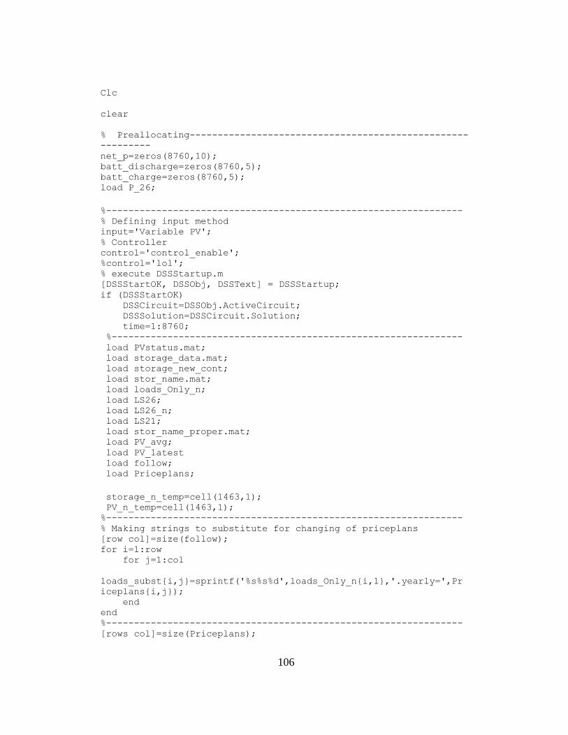
106
Clc
clear
% Preallocating--------------------------------------------------
--------- net_p=zeros(8760,10); batt_discharge=zeros(8760,5); batt_charge=zeros(8760,5); load P_26;
%---------------------------------------------------------------- % Defining input method input='Variable PV'; % Controller control='control_enable'; %control='lol'; % execute DSSStartup.m [DSSStartOK, DSSObj, DSSText] = DSSStartup; if (DSSStartOK) DSSCircuit=DSSObj.ActiveCircuit; DSSSolution=DSSCircuit.Solution; time=1:8760; %--------------------------------------------------------------- load PVstatus.mat; load storage_data.mat; load storage_new_cont; load stor_name.mat; load loads_Only_n; load LS26; load LS26_n; load LS21; load stor_name_proper.mat; load PV_avg; load PV_latest load follow; load Priceplans;
storage_n_temp=cell(1463,1); PV_n_temp=cell(1463,1); %---------------------------------------------------------------- % Making strings to substitute for changing of priceplans [row col]=size(follow); for i=1:row for j=1:col
loads_subst{i,j}=sprintf('%s%s%d',loads_Only_n{i,1},'.yearly=',Pr
iceplans{i,j}); end end %---------------------------------------------------------------- [rows col]=size(Priceplans);

107
% For 2kW PV and 1kW storage load--------------------------------
---------- for i=1 count=1; for count=5 %----------------------------------------------------------------
---------- % if (count==1) % factor=3.0; end % if (count==2) % factor=3.2; end % if (count==3) % factor=3.4; end % if (count==4) % factor=3.6; end % if (count==5) % factor=3.8; end %---------------------------------------------------------------
---------- year{i,1}=sprintf('%s %d','Set year=',i);
DSSText.Command ='Compile (C:\Users\Aditya\Desktop\DSS
files\Master_n_mat.txt)';
DSSText.Command ='set casename=PV_pen'; DSSText.Command ='Set MaxControlIter=30'; DSSText.Command ='Set stepsize=3600'; DSSText.Command =year{i,1}; DSSText.Command ='set mode=yearly hour =0 Number =8760';
%--------------------------------------------------------------- for k=1:size(storage_data)
storage_n_temp{k,1}=sprintf('%s%s',storage_new_cont{k,1},PVstatus
{k,i}); end
% Specify the inputs load_kW=4; kWTarget=load_kW; mult=0.6; %--------------------------------------------------------------- % Loading the matrices load PV_avg; load LS26;
% Defining the load rating DSSText.Command=sprintf('%s=
%d','Load.0x00899528_1_1.kW',load_kW); DSSText.Command=sprintf('%s=
%d','Load.0x00899528_1_1.yearly',26); LS26=LS26*load_kW;

108
% Defining PV system rating if strcmp('Variable PV',input) %PV_avg= 2*factor*PV_avg; PV_avg= 7.5*PV_avg; else PV_avg=PV_avg*4; end
% Defining storage ratings stor_kW=4; stor_kWh=20.70;
for f=1:8760
% Charging if LS26(f,1)-PV_avg(f,1)<=0 batt_charge(f,count)=-(PV_avg(f,1)-LS26(f,1))/stor_kW; only_PV(f,count)=0; net_p(f,count)=(LS26(f,1)-PV_avg(f,1)); if net_p(f,count)>10 net_p(f,count)=10; end end
if (LS26(f,1)-PV_avg(f,1)>0) only_PV(f,count)=LS26(f,1)-(PV_avg(f,1)); end
%---------------------------------------------------------------
---------- % discharge values if load_kW==4 load total_p_orig; end
if load_kW==6 load total_p_orig; total_p_orig=total_p_orig*3/2; end
if load_kW==8 load total_p_orig; total_p_orig=total_p_orig*2; end
% Summer if (f>=3625 && f<=5832) if (total_p_orig(f,1)-PV_avg(f,1)>mult*kWTarget) list_s(f,count)=1; batt_charge(f,count)=(total_p_orig(f,1)-PV_avg(f,1)-
mult*kWTarget)/stor_kW;
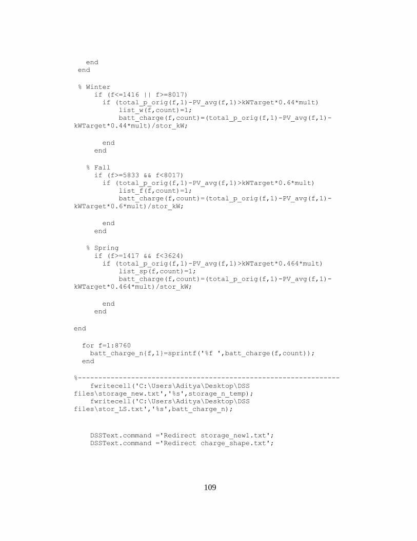
109
end end
% Winter if (f<=1416 || f>=8017) if (total_p_orig(f,1)-PV_avg(f,1)>kWTarget*0.44*mult) list_w(f,count)=1; batt_charge(f,count)=(total_p_orig(f,1)-PV_avg(f,1)-
kWTarget*0.44*mult)/stor_kW;
end end
% Fall if (f>=5833 && f<8017) if (total_p_orig(f,1)-PV_avg(f,1)>kWTarget*0.6*mult) list_f(f,count)=1; batt_charge(f,count)=(total_p_orig(f,1)-PV_avg(f,1)-
kWTarget*0.6*mult)/stor_kW;
end end
% Spring if (f>=1417 && f<3624) if (total_p_orig(f,1)-PV_avg(f,1)>kWTarget*0.464*mult) list_sp(f,count)=1; batt_charge(f,count)=(total_p_orig(f,1)-PV_avg(f,1)-
kWTarget*0.464*mult)/stor_kW;
end end
end
for f=1:8760 batt_charge_n{f,1}=sprintf('%f ',batt_charge(f,count)); end
%---------------------------------------------------------------- fwritecell('C:\Users\Aditya\Desktop\DSS
files\storage_new.txt','%s',storage_n_temp); fwritecell('C:\Users\Aditya\Desktop\DSS
files\stor_LS.txt','%s',batt_charge_n);
DSSText.command ='Redirect storage_new1.txt'; DSSText.command ='Redirect charge_shape.txt';

110
DSSText.Command =sprintf('%s.kWrated=%d','storage.Li-
ion_0x00899528_drop-1-1',stor_kW); DSSText.Command =sprintf('%s.kWhrated=%d','storage.Li-
ion_0x00899528_drop-1-1',stor_kWh); DSSText.Command ='storage.Li-ion_0x00899528_drop-1-
1.%EffCharge=92.5'; DSSText.Command ='storage.Li-ion_0x00899528_drop-1-
1.%EffdisCharge=92.5';
if strcmp('control_enable',control) DSSText.Command ='Redirect stor_control_peakshave.txt';
DSSText.Command=sprintf('%s','StorageController.main.modedischarg
e=loadshape');
DSSText.Command=sprintf('%s','StorageController.main.modecharge=l
oadshape');
DSSText.Command=sprintf('%s=%d','StorageController.main.kWTarget'
,load_kW*mult);
end
%----------------------------------------------------------------
----------
% Defining monitors and energymeter at the substation end
DSSText.command='New monitor.load1_s
element=Load.0x00899528_1_1 terminal=1 mode=1 PPolar=No'; DSSText.command='New monitor.stor1_s element=storage.Li-
ion_0x00899528_drop-1-1 terminal=1 mode=1 PPolar=No'; DSSText.command='New monitor.storage_line_s
element=Line.0x00899528_drop-1-1 terminal=1 mode=1 PPolar=No ';
%----------------------------------------------------------------
---------- DSSSolution.Solve; %DSSText.Command='show eventlog'; %----------------------------------------------------------------
----------
DSSText.Command='Export Monitor load1_s'; DSSText.Command='Export Monitor storage_line_s';
%----------------------------------------------------------------
---------- % Reading in monitors
MyCSV13=csvread('C:\Users\Aditya\Desktop\DSS
files\PV_pen_Mon_storage_line_s.csv',1,1);

111
MyCSV14=csvread('C:\Users\Aditya\Desktop\DSS
files\PV_pen_Mon_load1_s.csv',1,1);
%----------------------------------------------------------------
---------- % Saving data to MATLAB
% 1) Line data total_p(:,count)=MyCSV13(:,2)+MyCSV13(:,4);
stor_PV(:,count)=only_PV(:,count);
for f=1:8760
% summer if (f>=3625 && f<=5832) if (abs(total_p(f,count)-mult*kWTarget)<=0.1 &&
batt_charge(f,count)>0) list1(f,count)=1; batt_discharge(f,count)=total_p_orig(f,1)-
total_p(f,count); stor_PV(f,count)=total_p(f,count); end end
% winter if (f<=1416 || f>=8017) if (abs(total_p(f,count)-mult*0.44*kWTarget)<=0.1 &&
batt_charge(f,count)>0) list1(f,count)=1; batt_discharge(f,count)=total_p_orig(f,1)-
total_p(f,count); stor_PV(f,count)=total_p(f,count); end end
% Fall if (f>=5833 && f<8017) if (abs(total_p(f,count)-mult*0.6*kWTarget)<=0.1 &&
batt_charge(f,count)>0) list1(f,count)=1; batt_discharge(f,count)=total_p_orig(f,1)-
total_p(f,count); stor_PV(f,count)=total_p(f,count); end end
% Spring if (f>=1417 && f<3624)

112
if (abs(total_p(f,count)-mult*0.464*kWTarget)<=0.1 &&
batt_charge(f,count)>0) list1(f,count)=1; batt_discharge(f,count)=total_p_orig(f,1)-
total_p(f,count); stor_PV(f,count)=total_p(f,count); end end
end
%----------------------------------------------------------------
---------%
%----------------------------------------------------------------
---------% % Three cases
% Case I) Original system
for f=1:8760 basebill(f,1)=LS26(f,1)*P_26(f,1)/2; end
%----------------------------------------------------------------
---------- % Case II) Only PV
for f=1:8760
onlyPV_charge(f,count)=only_PV(f,count)*P_26(f,1)/2; onlyPV_savings(f,count)=basebill(f,1)-
onlyPV_charge(f,count);
if net_p(f,count)<0 net_metsavings_orig(f,count)=-net_p(f,count)*(0.03765-
0.00017)/2; % %onlyPV_savings(f,count)=(onlyPV_savings(f,count)))%-
(net_p(f,count)*(0.03765-0.00017))/2; end
end flag=0;
%----------------------------------------------------------------
---------
% Case III) PV + storage (Annual)
%batt_discharge(:,count)=only_PV(:,count)-stor_PV(:,count);

113
for f=1:8760 storPV_charge(f,count)=stor_PV(f,count)*P_26(f,1)/2; storPV_savings(f,count)=basebill(f,1)-storPV_charge(f,count); end
stor_PV_act= stor_PV/2;
if count==2 u= stor_PV_act(:,count); us=storPV_savings(:,count); end
if count==3 v= stor_PV_act(:,count); vs=storPV_savings(:,count); end
if count==4 w= stor_PV_act(:,count); ws=storPV_savings(:,count); end
if count==5 x= stor_PV_act(:,count); xs=storPV_savings(:,count); end %----------------------------------------------------------------
---------
end end end
%----------------------------------------------------------------
---------
load PV_avg; for i=1:2 % netmet_total(i,1)=-sum(net_metsavings(:,i)); onlyPV_savings_total(i,1)=sum(onlyPV_savings(:,i)); storPV_savings_total(i,1)=sum(storPV_savings(:,i)); netmet_savings_total(i,1)=sum(net_metsavings_orig(:,i)); kWh_total(:,i)=i*sum(PV_avg(:,1)); end
for i=1:2 reduction(:,i)=only_PV(:,i)-stor_PV(:,i); end

114
reduction_input=reduction/0.856; netmet_savings=reduction_input*(0.037-0.00017)/2;
for i=1:2 netmet_annual(i,1)=sum(netmet_savings(:,i)); end
k=1; discharge=zeros(365,5); charge=zeros(365,5); for count=1:2 k=1; for i=1:365
for j=1:24
if batt_charge(k,count)<0 charge(i,count)=charge(i,count)+batt_charge(k,count);
end k=k+1; end end
end charge=-charge*stor_kW;
%----------------------------------------------------------------
----------
total_onlyPV=onlyPV_savings_total+netmet_savings_total; total_onlystor=storPV_savings_total+netmet_savings_total-
netmet_annual;

115
APPENDIX B
SUNVERGE SIS 2.0 DATASHEET
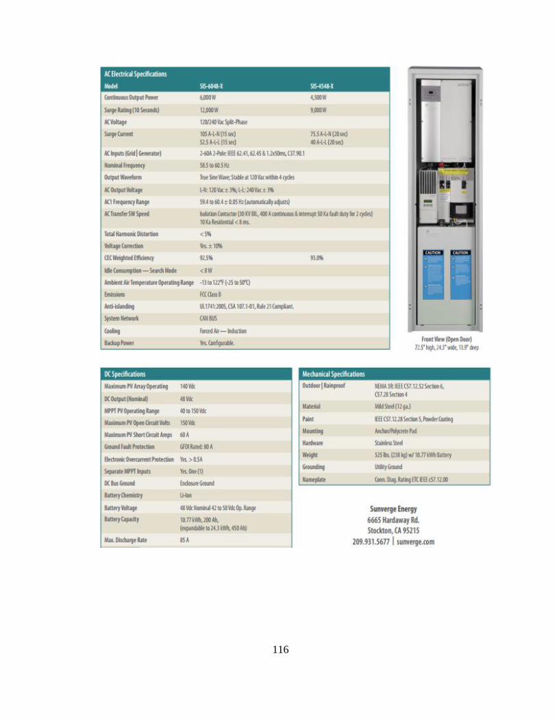
116

117
APPENDIX C
EXCEL SHEET FOR CALCULATING PV AND STORAGE SYSTEM LIFE
CYCLE COST