Embed Size (px)
Citation preview
Journal of Computational and Applied Mathematics 196 (2006) 553–566www.elsevier.com/locate/cam
A telescoping method for double summationsWilliam Y.C. Chen∗, Qing-Hu Hou, Yan-Ping MuCenter for Combinatorics, LPMC, Nankai University, Tianjin 300071, PR China
Received 25 April 2005; received in revised form 4 September 2005
Dedicated to James D. Louck on the occasion of his seventy-fifth birthday
Abstract
We present a method to prove hypergeometric double summation identities. Given a hypergeometric term F(n, i, j), we aimto find a difference operator L = a0(n)N0 + a1(n)N1 + · · · + ar (n)Nr and rational functions R1(n, i, j), R2(n, i, j) such thatLF =�i (R1F)+�j (R2F). Based on simple divisibility considerations, we show that the denominators of R1 and R2 must possesscertain factors which can be computed from F(n, i, j). Using these factors as estimates, we may find the numerators of R1 and R2 byguessing the upper bounds of the degrees and solving systems of linear equations. Our method is valid for theAndrews–Paule identity,Carlitz’s identities, the Apéry–Schmidt–Strehl identity, the Graham–Knuth–Patashnik identity, and the Petkovšek–Wilf–Zeilbergeridentity.© 2005 Elsevier B.V. All rights reserved.
MSC: 33F10; 68W30
Keywords: Zeilberger’s algorithm; Double summation; Hypergeometric term
1. Introduction
This paper is concerned with double summations of hypergeometric terms F(n, i, j). A function F(n, k1, . . . , km)
is called a hypergeometric term if the quotients
F(n + 1, k1, . . . , km)
F (n, k1, . . . , km),F (n, k1 + 1, . . . , km)
F (n, k1, . . . , km), . . . ,
F (n, k1, . . . , km + 1)
F (n, k1, . . . , km)
are rational functions of n, k1, . . . , km. Throughout the paper, we use N to denote the shift operator with respect to thevariable n, given by NF(n) = F(n + 1) and use �x to denote the difference operator with respect to the variable x,given by �xF = F(x + 1) − F(x). For polynomials a and b, we denote by gcd(a, b) their monic greatest commondivisor. When we express a rational function as a quotient p/q, we always assume that p and q are relatively primeunless it is explicitly stated otherwise.
∗ Corresponding author. Tel.: +86 22 2350 2180; fax: +86 22 2350 9272.E-mail addresses: [email protected] (W.Y.C. Chen), [email protected] (Q.-H. Hou), [email protected] (Y.-P. Mu).
0377-0427/$ - see front matter © 2005 Elsevier B.V. All rights reserved.doi:10.1016/j.cam.2005.10.010
554 W.Y.C. Chen et al. / Journal of Computational and Applied Mathematics 196 (2006) 553 –566
Zeilberger’s algorithm [14,17,22], also known as the method of creative telescoping, is devised for proving hyper-geometric identities of the form∑
k
F (n, k) = f (n), (1.1)
where F(n, k) is a hypergeometric term and f (n) is a given function. This algorithm has been used to deal with multiplesums in [21]. Given a hypergeometric term F(n, k1, . . . , km), the approach of Wilf and Zeilberger tries to find a lineardifference operator L with coefficients being polynomials in n
L = a0(n)N0 + a1(n)N1 + · · · + ar(n)Nr
and rational functions R1, . . . , Rm of n, k1, . . . , km such that
LF =m∑
l=1
�kl(RlF ). (1.2)
As noted by Wegschaider [20], when the boundary conditions are admissible, Eq. (1.2) leads to a homogenous recursionfor the multi-summations:
L∑
k1,...,km
F (n, k1, . . . , km) = 0.
When m = 1, L and R1 can be solved by Gosper’s algorithm [13,17]. Abramov, Geddes and Le also provided alower bound for the order r [2,3] and found a faster algorithm [4] compared with Zeilberger’s algorithm. For a surveyon recent developments, see [1]. For m�2, constructing the denominators of R1, . . . , Rm for the Wilf–Zeilbergerapproach remains an open problem. In a recent paper [16], Mohammed and Zeilberger used the denominator of LF/F
as estimates of the denominators of Ri . In an alternative approach, Wegschaider generalized Sister Celine’s technique[20] to multiple summations, and proved many double summation identities. A different approach has been proposedby Chyzak [11,12] by finding recursions of the summation iteratively starting from the inner sum. Schneider [18]presented the Chyzak method from the point of view of Karr’s difference field theory.
To give a sketch of our approach, we first consider Gosper’s algorithm for bivariate hypergeometric terms. Supposethat F(i, j) is a hypergeometric term and p1/q1, p2/q2 are rational functions such that
F(i, j) = �i
(p1(i, j)
q1(i, j)F (i, j)
)+ �j
(p2(i, j)
q2(i, j)F (i, j)
).
We show that under certain hypotheses (Section 2, (H1)–(H3)), the denominators q1, q2 can be written in the form
q1(i, j) = v1(i) v2(j) v3(i + j) v4(i, j) u1(j) u2(i, j),
q2(i, j) = v1(i) v2(j) v3(i + j) v4(i, j)w1(i)w2(i, j), (1.3)
such that v1, v2, v4 and u2, w2 are bounded in the sense that they are factors of certain polynomials which can becomputed for a given F(i, j), see Theorem 2.1. Then we apply these estimates to the telescoping algorithm for doublesummations. Suppose that
LF(n, i, j) = �i (R1(n, i, j)F (n, i, j)) + �j (R2(n, i, j)F (n, i, j)),
where
R1(n, i, j) = 1
d(n, i, j)· f1(n, i, j)
g1(n, i, j), R2(n, i, j) = 1
d(n, i, j)· f2(n, i, j)
g2(n, i, j)
and d(n, i, j) is the denominator of LF(n, i, j)/F (n, i, j). We may deduce that g1, g2 can be factored in the form of(1.3) such that v1, v2, v4 and u2, w2 are bounded, see Theorem 3.1.Although we do not have the universal denominators,these bounds can be used to give estimates of the denominators g1 and g2. Then by further guessing the bounds of thedegrees of the numerators of R1 and R2, we get the desired difference operator if we are lucky.
Indeed, our approach works quite efficiently for many identities such as the Andrews–Paule identity, Carlitz’s iden-tities, the Apéry–Schmidt–Strehl identity, the Graham–Knuth–Patashnik identity, and the Petkovšek–Wilf–Zeilbergeridentity.
W.Y.C. Chen et al. / Journal of Computational and Applied Mathematics 196 (2006) 553 –566 555
2. Denominators in bivariate Gosper’s algorithm
For a given bivariate hypergeometric term F(i, j), we give estimates of the denominators of the rational functionsR1(i, j), R2(i, j) satisfying
F(i, j) = �i (R1(i, j)F (i, j)) + �j (R2(i, j)F (i, j)). (2.1)
Let
R1(i, j) = f1(i, j)
g1(i, j), R2(i, j) = f2(i, j)
g2(i, j),
F(i + 1, j)
F (i, j)= r1(i, j)
s1(i, j),
F (i, j + 1)
F (i, j)= r2(i, j)
s2(i, j). (2.2)
Dividing F(i, j) on both sides of (2.1) and substituting (2.2) into it, we derive that
1 = r1(i, j)
s1(i, j)
f1(i + 1, j)
g1(i + 1, j)− f1(i, j)
g1(i, j)+ r2(i, j)
s2(i, j)
f2(i, j + 1)
g2(i, j + 1)− f2(i, j)
g2(i, j). (2.3)
Let
u(i, j) = gcd(s1(i, j), s2(i, j)), v(i, j) = gcd(g1(i, j), g2(i, j)),
and
s′1(i, j) = s1(i, j)/u(i, j), s′
2(i, j) = s2(i, j)/u(i, j),
g′1(i, j) = g1(i, j)/v(i, j), g′
2(i, j) = g2(i, j)/v(i, j). (2.4)
We find that in many cases we can restrict our attention to those R1, R2 whose denominators g1, g2 satisfy thefollowing three hypotheses. We see that in the proof of the following theorem, these hypotheses enable us to cancelout unknown factors from the multiples of g1 and g2 so that we can obtain an upper bound of g1 and g2. Thus, thesehypotheses come naturally from the requirement of simple divisibility properties. Moreover, it turns out that thesedivisibility requirements are sufficient in many cases to give good estimates for the denominators g1 and g2. The threehypotheses are as follows:
(H1) Suppose p(i, j) and p(i + h1, j + h2) are both irreducible factors of g1(i, j) (g2(i, j), respectively) for someh1, h2 ∈ {−1, 0, 1}. Then they must be coincide.
(H2) gcd(g′1(i, j), v(i, j)) = gcd(g′
2(i, j), v(i, j)) = 1.(H3) For any integers h1, h2 ∈ {−1, 0, 1},
gcd(g′1(i + h1, j + h2), g
′2(i, j)) = 1.
For example, the following functions satisfy the above hypotheses:
g1(i, j) = (2n − 2i + 1)(n − i + 1)(j + 1)2, g2(i, j) = (2n − 2i + 1)(n − i + 1)(i + 1)2.
Remarks. 1. Hypothesis (H1) looks like requiring that g1 and g2 are shift-free (see [5]). However, only the shifts of±1 are considered and shift invariant factors are admissible. For example, we allow that g1(i, j) = (i + 1)(i + 3) org1(i, j) = i + j .
2.According to [6], gcd(g1(i, j), g1(i+h1, j+h2)) and gcd(g2(i, j), g2(i+h1, j+h2)) can factor into integer-linearfactors for h1, h2 being not both zero.
3. Hypothesis (H3) is to require that g′1/g
′2 are shift-reduced (see also [5]) respect to the shifts of ±1.
Under the above hypotheses, we have
556 W.Y.C. Chen et al. / Journal of Computational and Applied Mathematics 196 (2006) 553 –566
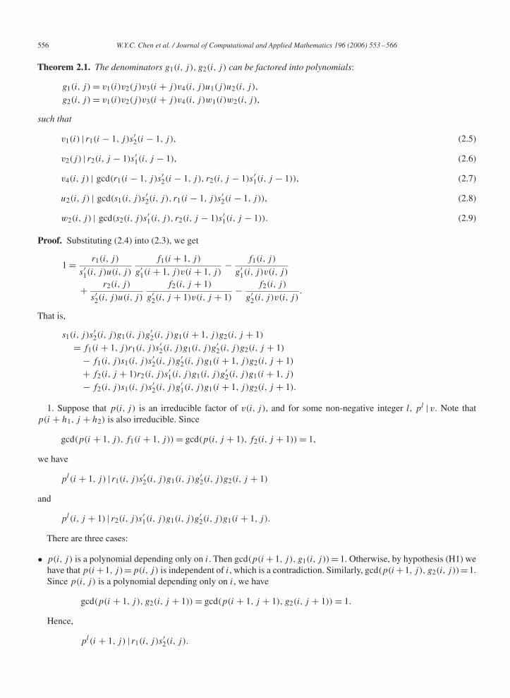
Theorem 2.1. The denominators g1(i, j), g2(i, j) can be factored into polynomials:
g1(i, j) = v1(i)v2(j)v3(i + j)v4(i, j)u1(j)u2(i, j),
g2(i, j) = v1(i)v2(j)v3(i + j)v4(i, j)w1(i)w2(i, j),
such that
v1(i) | r1(i − 1, j)s′2(i − 1, j), (2.5)
v2(j) | r2(i, j − 1)s′1(i, j − 1), (2.6)
v4(i, j) | gcd(r1(i − 1, j)s′2(i − 1, j), r2(i, j − 1)s′
1(i, j − 1)), (2.7)
u2(i, j) | gcd(s1(i, j)s′2(i, j), r1(i − 1, j)s′
2(i − 1, j)), (2.8)
w2(i, j) | gcd(s2(i, j)s′1(i, j), r2(i, j − 1)s′
1(i, j − 1)). (2.9)
Proof. Substituting (2.4) into (2.3), we get
1 = r1(i, j)
s′1(i, j)u(i, j)
f1(i + 1, j)
g′1(i + 1, j)v(i + 1, j)
− f1(i, j)
g′1(i, j)v(i, j)
+ r2(i, j)
s′2(i, j)u(i, j)
f2(i, j + 1)
g′2(i, j + 1)v(i, j + 1)
− f2(i, j)
g′2(i, j)v(i, j)
.
That is,
s1(i, j)s′2(i, j)g1(i, j)g′
2(i, j)g1(i + 1, j)g2(i, j + 1)
= f1(i + 1, j)r1(i, j)s′2(i, j)g1(i, j)g′
2(i, j)g2(i, j + 1)
− f1(i, j)s1(i, j)s′2(i, j)g′
2(i, j)g1(i + 1, j)g2(i, j + 1)
+ f2(i, j + 1)r2(i, j)s′1(i, j)g1(i, j)g′
2(i, j)g1(i + 1, j)
− f2(i, j)s1(i, j)s′2(i, j)g′
1(i, j)g1(i + 1, j)g2(i, j + 1).
1. Suppose that p(i, j) is an irreducible factor of v(i, j), and for some non-negative integer l, pl | v. Note thatp(i + h1, j + h2) is also irreducible. Since
gcd(p(i + 1, j), f1(i + 1, j)) = gcd(p(i, j + 1), f2(i, j + 1)) = 1,
we have
pl(i + 1, j) | r1(i, j)s′2(i, j)g1(i, j)g′
2(i, j)g2(i, j + 1)
and
pl(i, j + 1) | r2(i, j)s′1(i, j)g1(i, j)g′
2(i, j)g1(i + 1, j).
There are three cases:
• p(i, j) is a polynomial depending only on i. Then gcd(p(i + 1, j), g1(i, j)) = 1. Otherwise, by hypothesis (H1) wehave that p(i +1, j)=p(i, j) is independent of i, which is a contradiction. Similarly, gcd(p(i +1, j), g2(i, j))=1.Since p(i, j) is a polynomial depending only on i, we have
gcd(p(i + 1, j), g2(i, j + 1)) = gcd(p(i + 1, j + 1), g2(i, j + 1)) = 1.
Hence,
pl(i + 1, j) | r1(i, j)s′2(i, j).
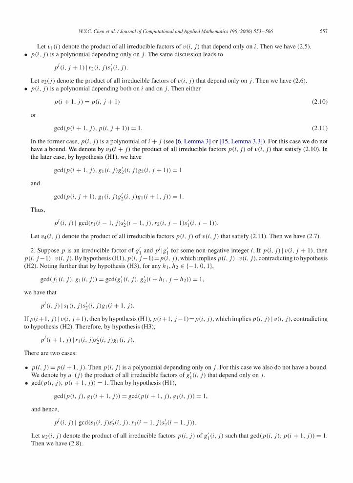
W.Y.C. Chen et al. / Journal of Computational and Applied Mathematics 196 (2006) 553 –566 557
Let v1(i) denote the product of all irreducible factors of v(i, j) that depend only on i. Then we have (2.5).• p(i, j) is a polynomial depending only on j . The same discussion leads to
pl(i, j + 1) | r2(i, j)s′1(i, j).
Let v2(j) denote the product of all irreducible factors of v(i, j) that depend only on j . Then we have (2.6).• p(i, j) is a polynomial depending both on i and on j . Then either
p(i + 1, j) = p(i, j + 1) (2.10)
or
gcd(p(i + 1, j), p(i, j + 1)) = 1. (2.11)
In the former case, p(i, j) is a polynomial of i + j (see [6, Lemma 3] or [15, Lemma 3.3]). For this case we do nothave a bound. We denote by v3(i + j) the product of all irreducible factors p(i, j) of v(i, j) that satisfy (2.10). Inthe later case, by hypothesis (H1), we have
gcd(p(i + 1, j), g1(i, j)g′2(i, j)g2(i, j + 1)) = 1
and
gcd(p(i, j + 1), g1(i, j)g′2(i, j)g1(i + 1, j)) = 1.
Thus,
pl(i, j) | gcd(r1(i − 1, j)s′2(i − 1, j), r2(i, j − 1)s′
1(i, j − 1)).
Let v4(i, j) denote the product of all irreducible factors p(i, j) of v(i, j) that satisfy (2.11). Then we have (2.7).
2. Suppose p is an irreducible factor of g′1 and pl |g′
1 for some non-negative integer l. If p(i, j) | v(i, j + 1), thenp(i, j −1) | v(i, j). By hypothesis (H1), p(i, j −1)=p(i, j), which implies p(i, j) | v(i, j), contradicting to hypothesis(H2). Noting further that by hypothesis (H3), for any h1, h2 ∈ {−1, 0, 1},
gcd(f1(i, j), g1(i, j)) = gcd(g′1(i, j), g′
2(i + h1, j + h2)) = 1,
we have that
pl(i, j) | s1(i, j)s′2(i, j)g1(i + 1, j).
If p(i+1, j) | v(i, j +1), then by hypothesis (H1), p(i+1, j −1)=p(i, j), which implies p(i, j) | v(i, j), contradictingto hypothesis (H2). Therefore, by hypothesis (H3),
pl(i + 1, j) | r1(i, j)s′2(i, j)g1(i, j).
There are two cases:
• p(i, j) = p(i + 1, j). Then p(i, j) is a polynomial depending only on j . For this case we also do not have a bound.We denote by u1(j) the product of all irreducible factors of g′
1(i, j) that depend only on j .• gcd(p(i, j), p(i + 1, j)) = 1. Then by hypothesis (H1),
gcd(p(i, j), g1(i + 1, j)) = gcd(p(i + 1, j), g1(i, j)) = 1,
and hence,
pl(i, j) | gcd(s1(i, j)s′2(i, j), r1(i − 1, j)s′
2(i − 1, j)).
Let u2(i, j) denote the product of all irreducible factors p(i, j) of g′1(i, j) such that gcd(p(i, j), p(i + 1, j)) = 1.
Then we have (2.8).
558 W.Y.C. Chen et al. / Journal of Computational and Applied Mathematics 196 (2006) 553 –566
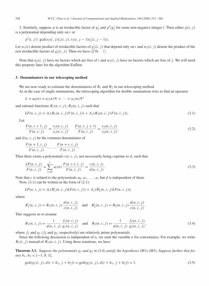
3. Similarly, suppose p is an irreducible factor of g′2 and pl |g′
2 for some non-negative integer l. Then either p(i, j)
is a polynomial depending only on i or
pl(i, j) | gcd(s2(i, j)s′1(i, j), r2(i, j − 1)s′
1(i, j − 1)).
Let w1(i) denote product of irreducible factors of g′2(i, j) that depend only on i and w2(i, j) denote the product of the
rest irreducible factors of g′2(i, j). Then we have (2.9). �
Note that u2(i, j) have no factors which are free of i and w2(i, j) have no factors which are free of j . We will needthis property later for the algorithm EstDen.
3. Denominators in our telescoping method
We are now ready to estimate the denominators of R1 and R2 in our telescoping method.As in the case of single summations, the telescoping algorithm for double summations tries to find an operator
L = a0(n) + a1(n)N + · · · + ar(n)Nr
and rational functions R1(n, i, j), R2(n, i, j) such that
LF(n, i, j) = �i (R1(n, i, j)F (n, i, j)) + �j (R2(n, i, j)F (n, i, j)). (3.1)
Let
F(n, i + 1, j)
F (n, i, j)= r1(n, i, j)
s1(n, i, j),
F (n, i, j + 1)
F (n, i, j)= r2(n, i, j)
s2(n, i, j), (3.2)
and d(n, i, j) be the common denominator of
F(n + 1, i, j)
F (n, i, j), . . . ,
F (n + r, i, j)
F (n, i, j).
Then there exists a polynomial c(n, i, j), not necessarily being coprime to d, such that
LF(n, i, j)
F (n, i, j)=
r∑l=0
al(n)F (n + l, i, j)
F (n, i, j)= c(n, i, j)
d(n, i, j). (3.3)
Note that c is related to the polynomials a0, a1, . . . , ar but d is independent of them.Now, (3.1) can be written in the form of (2.1):
LF(n, i, j) = �i (R′1(n, i, j)LF(n, i, j)) + �j (R
′2(n, i, j)LF(n, i, j)),
where
R′1(n, i, j) = R1(n, i, j)
d(n, i, j)
c(n, i, j)and R′
2(n, i, j) = R2(n, i, j)d(n, i, j)
c(n, i, j).
This suggests us to assume
R1(n, i, j) = 1
d(n, i, j)
f1(n, i, j)
g1(n, i, j)and R2(n, i, j) = 1
d(n, i, j)
f2(n, i, j)
g2(n, i, j), (3.4)
where f1 and g1 (f2 and g2, respectively) are relatively prime polynomials.Since the following discussion is independent of n, we omit the variable n for convenience. For example, we write
R1(i, j) instead of R1(n, i, j). Using these notations, we have
Theorem 3.1. Suppose the polynomials g1 and g2 in (3.4) satisfy the hypotheses (H1)–(H3). Suppose further that forany h1, h2 ∈ {−1, 0, 1},
gcd(g1(i, j), d(i + h1, j + h2)) = gcd(g2(i, j), d(i + h1, j + h2)) = 1. (3.5)
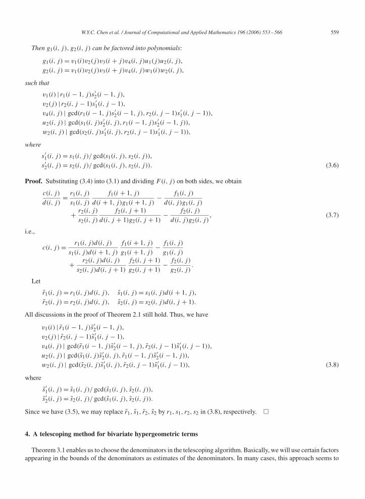
W.Y.C. Chen et al. / Journal of Computational and Applied Mathematics 196 (2006) 553 –566 559
Then g1(i, j), g2(i, j) can be factored into polynomials:
g1(i, j) = v1(i)v2(j)v3(i + j)v4(i, j)u1(j)u2(i, j),
g2(i, j) = v1(i)v2(j)v3(i + j)v4(i, j)w1(i)w2(i, j),
such that
v1(i) | r1(i − 1, j)s′2(i − 1, j),
v2(j) | r2(i, j − 1)s′1(i, j − 1),
v4(i, j) | gcd(r1(i − 1, j)s′2(i − 1, j), r2(i, j − 1)s′
1(i, j − 1)),
u2(i, j) | gcd(s1(i, j)s′2(i, j), r1(i − 1, j)s′
2(i − 1, j)),
w2(i, j) | gcd(s2(i, j)s′1(i, j), r2(i, j − 1)s′
1(i, j − 1)),
where
s′1(i, j) = s1(i, j)/ gcd(s1(i, j), s2(i, j)),
s′2(i, j) = s2(i, j)/ gcd(s1(i, j), s2(i, j)). (3.6)
Proof. Substituting (3.4) into (3.1) and dividing F(i, j) on both sides, we obtain
c(i, j)
d(i, j)= r1(i, j)
s1(i, j)
f1(i + 1, j)
d(i + 1, j)g1(i + 1, j)− f1(i, j)
d(i, j)g1(i, j)
+ r2(i, j)
s2(i, j)
f2(i, j + 1)
d(i, j + 1)g2(i, j + 1)− f2(i, j)
d(i, j)g2(i, j), (3.7)
i.e.,
c(i, j) = r1(i, j)d(i, j)
s1(i, j)d(i + 1, j)
f1(i + 1, j)
g1(i + 1, j)− f1(i, j)
g1(i, j)
+ r2(i, j)d(i, j)
s2(i, j)d(i, j + 1)
f2(i, j + 1)
g2(i, j + 1)− f2(i, j)
g2(i, j).
Let
r̃1(i, j) = r1(i, j)d(i, j), s̃1(i, j) = s1(i, j)d(i + 1, j),
r̃2(i, j) = r2(i, j)d(i, j), s̃2(i, j) = s2(i, j)d(i, j + 1).
All discussions in the proof of Theorem 2.1 still hold. Thus, we have
v1(i) | r̃1(i − 1, j)s̃′2(i − 1, j),
v2(j) | r̃2(i, j − 1)s̃′1(i, j − 1),
v4(i, j) | gcd(r̃1(i − 1, j)s̃′2(i − 1, j), r̃2(i, j − 1)s̃′
1(i, j − 1)),
u2(i, j) | gcd(s̃1(i, j)s̃′2(i, j), r̃1(i − 1, j)s̃′
2(i − 1, j)),
w2(i, j) | gcd(s̃2(i, j)s̃′1(i, j), r̃2(i, j − 1)s̃′
1(i, j − 1)), (3.8)
where
s̃′1(i, j) = s̃1(i, j)/ gcd(s̃1(i, j), s̃2(i, j)),
s̃′2(i, j) = s̃2(i, j)/ gcd(s̃1(i, j), s̃2(i, j)).
Since we have (3.5), we may replace r̃1, s̃1, r̃2, s̃2 by r1, s1, r2, s2 in (3.8), respectively. �
4. A telescoping method for bivariate hypergeometric terms
Theorem 3.1 enables us to choose the denominators in the telescoping algorithm. Basically, we will use certain factorsappearing in the bounds of the denominators as estimates of the denominators. In many cases, this approach seems to
560 W.Y.C. Chen et al. / Journal of Computational and Applied Mathematics 196 (2006) 553 –566
work quite efficiently although we are not able to give a formula to bound the denominators because certain factors arenot bounded in Theorem 3.1. Roughly speaking, the divisibility considerations in our method serve as a guide to guessthe factors in the denominators. In fact, the estimated denominators are much smaller than the theoretical bounds givenby Theorem 3.1. Only u2(i, j) and w2(i, j) are set to their theoretical bounds, while v2(j), v3(i + j), v4(i, j) are setto 1, u1(j) and w1(i) are set to factors of s1(i, j)s′
2(i, j), and v1(i) is set to a factor of its theoretical bound. See thefollowing algorithm EstDen.
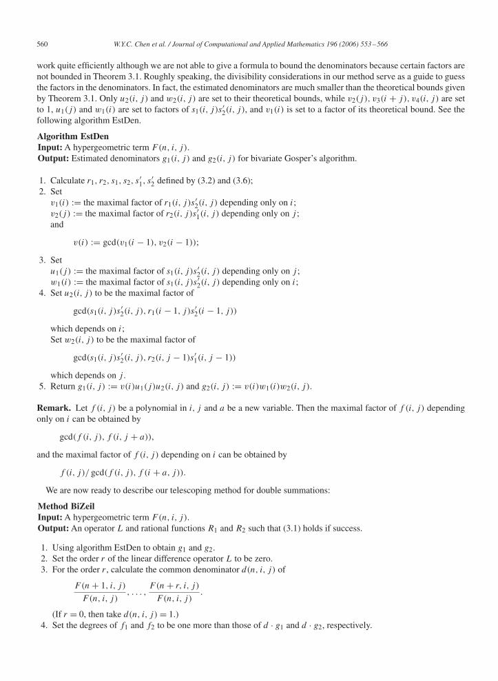
Algorithm EstDenInput: A hypergeometric term F(n, i, j).Output: Estimated denominators g1(i, j) and g2(i, j) for bivariate Gosper’s algorithm.
1. Calculate r1, r2, s1, s2, s′1, s
′2 defined by (3.2) and (3.6);
2. Setv1(i) := the maximal factor of r1(i, j)s′
2(i, j) depending only on i;v2(j) := the maximal factor of r2(i, j)s′
1(i, j) depending only on j ;and
v(i) := gcd(v1(i − 1), v2(i − 1));
3. Setu1(j) := the maximal factor of s1(i, j)s′
2(i, j) depending only on j ;w1(i) := the maximal factor of s1(i, j)s′
2(i, j) depending only on i;4. Set u2(i, j) to be the maximal factor of
gcd(s1(i, j)s′2(i, j), r1(i − 1, j)s′
2(i − 1, j))
which depends on i;Set w2(i, j) to be the maximal factor of
gcd(s1(i, j)s′2(i, j), r2(i, j − 1)s′
1(i, j − 1))
which depends on j .5. Return g1(i, j) := v(i)u1(j)u2(i, j) and g2(i, j) := v(i)w1(i)w2(i, j).
Remark. Let f (i, j) be a polynomial in i, j and a be a new variable. Then the maximal factor of f (i, j) dependingonly on i can be obtained by
gcd(f (i, j), f (i, j + a)),
and the maximal factor of f (i, j) depending on i can be obtained by
f (i, j)/ gcd(f (i, j), f (i + a, j)).
We are now ready to describe our telescoping method for double summations:
Method BiZeilInput: A hypergeometric term F(n, i, j).Output: An operator L and rational functions R1 and R2 such that (3.1) holds if success.
1. Using algorithm EstDen to obtain g1 and g2.2. Set the order r of the linear difference operator L to be zero.3. For the order r , calculate the common denominator d(n, i, j) of
F(n + 1, i, j)
F (n, i, j), . . . ,
F (n + r, i, j)
F (n, i, j).
(If r = 0, then take d(n, i, j) = 1.)4. Set the degrees of f1 and f2 to be one more than those of d · g1 and d · g2, respectively.
W.Y.C. Chen et al. / Journal of Computational and Applied Mathematics 196 (2006) 553 –566 561
5. Solve Eq. (3.7) by the method of undeterminate coefficients to obtain a0, a1, . . . , ar and f1, f2.6. If ai �= 0 for some i ∈ {0, . . . , r}, then return L, f1/(d · g1), f2/(d · g2) and we are done.
If ai = 0 for all i ∈ {0, . . . , r}, but deg f1 − deg(d · g1)�2, then increase the degrees of f1 and f2 by one andrepeat step 5.Otherwise, set r := r + 1 and repeat the process from step 3.
Remarks. 1. In many cases, g1(i, j) and g2(i, j) can be further reduced by cancelling a factor of degree 1 and afactor of degree 2 from g1 and g2, respectively. In our implementation we first choose two arbitrary factors and use thereduced g1 and g2. When it fails, we then try the unreduced ones. This cancellation may reduce the time of calculationif we are lucky. For example, for the Andrews–Paule identity (see Example 1), the estimated denominators given byTheorem 3.1, by algorithm EstDen, and by reduction are, respectively,
g1(i, j) = (2n − 2i + 1)(n − i + 1)(2n − 2j + 1)(n − j + 1)(i + j)2(j + 1)2,
g2(i, j) = (2n − 2i + 1)(n − i + 1)(2n − 2j + 1)(n − j + 1)(i + j)2(i + 1)2,
g1(i, j) = (2n − 2i + 1)(n − i + 1)(j + 1)2,
g2(i, j) = (2n − 2i + 1)(n − i + 1)(i + 1)2,
and
g1(i, j) = (2n − 2i + 1)(j + 1)2, g2(i, j) = (2n − 2i + 1)(n − i + 1).
The calculation times are 116 seconds, 5 seconds and 0.6 seconds, respectively. We should note that since our method isheuristic and it applies only to particular cases, we are more interested in the computation results which are verifiable.So we cannot claim the efficiency of the method or its applicability.
2. In all the following examples except Example 4, the degree of the numerator of R1 (R2) is one more than that ofthe denominator. While in Example 4, the difference is two.
The degree bounds can be interpreted as follows. Let t1, t2, t3, t4 be the four terms of the right-hand side of (3.7)after multiplying the common denominator. In most cases, the leading terms of t1 and t2 (t3 and t4, respectively) arecancelled.
3. There is a way to speed up the computation in Step 5. Given g1 and g2, we may derive part of the factors of f1and f2 by divisibility. For example, suppose (3.7) becomes
c(i, j)
d(i, j)= u1(i, j)
v1(i, j)f1(i + 1, j) − f1(i, j)
w1(i, j)+ u2(i, j)
v2(i, j)f2(i, j + 1) − f2(i, j)
w2(i, j),
after substituting and simplification. Suppose further that D(i, j) is the common denominator of the above equation.Then we immediately have that f1 · D/w1 is divisible by q1 = gcd(cD/d, u1D/v1, u2D/v2, D/w2) and f1(i + 1, j) ·u1D/v1 is divisible by q2 = gcd(cD/d, D/w1, u2D/v2, D/w2), and hence,
q1
gcd(D/w1, q1)and
q2
gcd(u1D/v1, q2)
are factors of f1(i, j) and f1(i + 1, j), respectively.
5. Examples
In the following examples, let F denote the summand of the left-hand side of the identity.
Example 1. The Andrews–Paule identity:
n∑i=0
n∑j=0
(i + j
i
)2 (4n − 2i − 2j
2n − 2i
)= (2n + 1)
(2n
n
)2
. (5.1)
562 W.Y.C. Chen et al. / Journal of Computational and Applied Mathematics 196 (2006) 553 –566
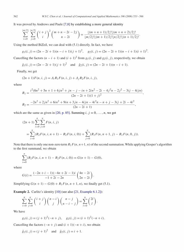
It was proved by Andrews and Paule [7,8] by establishing a more general identity
�m/2�∑i=0
�n/2�∑j=0
(i + j
i
)2 (m + n − 2i − 2j
n − 2i
)= �(m + n + 1)/2�!�(m + n + 2)/2�!
�m/2�!�(m + 1)/2�!�n/2�!�(n + 1)/2�! .
Using the method BiZeil, we can deal with (5.1) directly. In fact, we have
g1(i, j) = (2n − 2i + 1)(n − i + 1)(j + 1)2, g2(i, j) = (2n − 2i + 1)(n − i + 1)(i + 1)2.
Cancelling the factors (n − i + 1) and (i + 1)2 from g1(i, j) and g2(i, j), respectively, we obtain
g̃1(i, j) = (2n − 2i + 1)(j + 1)2 and g̃2(i, j) = (2n − 2i + 1)(n − i + 1).
Finally, we get
(2n + 1)F (n, i, j) = �iR1F(n, i, j) + �jR2F(n, i, j),
where
R1 = i2(6n2 + 5n + 1 + 6jn2 + jn − j − in + 2in2 − 2i − 4j2n − 2j2 − 3ij − 4ijn)
(2n − 2i + 1)(1 + j)2 ,
R2 = −2n2 + 2jn2 + 6in2 + 9in + 3jn − 4ijn − 4i2n − n + j − 3ij + 2i − 4i2
(2n − 2i + 1),
which are the same as given in [20, p. 85]. Summing i, j = 0, . . . , n, we get
(2n + 1)
n∑i=0
n∑j=0
F(n, i, j)
=n∑
i=0
(R2F(n, i, n + 1) − R2F(n, i, 0)) +n∑
j=0
(R1F(n, n + 1, j) − R1F(n, 0, j)).
Note that there is only one non-zero term R1F(n, n+1, n) of the second summation. While applying Gosper’s algorithmto the first summand, we obtain
n∑i=0
(R2F(n, i, n + 1) − R2F(n, i, 0)) = G(n + 1) − G(0),
where
G(i) = (−2n + i − 1)(−4n + 2i − 1)i
−1 + 2i − 2n
(4n − 2i
2n − 2i
).
Simplifying G(n + 1) − G(0) + R1F(n, n + 1, n), we finally get (5.1).
Example 2. Carlitz’s identity [10] (see also [21, Example 6.1.2]):
n∑i=0
n∑j=0
(i + j
i
) (n − i
j
) (n − j
n − i − j
)=
n∑l=0
(2l
l
).
We have
g1(i, j) = (j + 1)2(−n + j), g2(i, j) = (i + 1)2(−n + i).
Cancelling the factors (−n + j) and (i + 1)(−n + i), we obtain
g̃1(i, j) = (j + 1)2 and g̃2(i, j) = i + 1.
W.Y.C. Chen et al. / Journal of Computational and Applied Mathematics 196 (2006) 553 –566 563
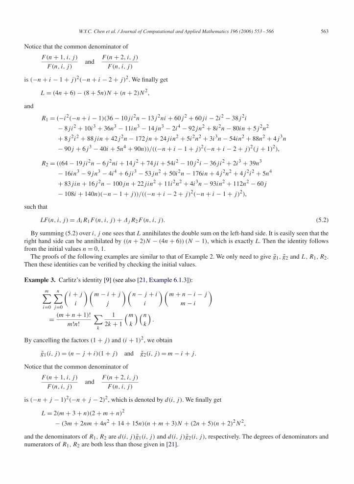
Notice that the common denominator of
F(n + 1, i, j)
F (n, i, j)and
F(n + 2, i, j)
F (n, i, j)
is (−n + i − 1 + j)2(−n + i − 2 + j)2. We finally get
L = (4n + 6) − (8 + 5n)N + (n + 2)N2,
and
R1 = (−i2(−n + i − 1)(36 − 10ji2n − 13j2ni + 60j2 + 60ji − 2i2 − 38j2i
− 8ji2 + 10i3 + 36n3 − 11in3 − 14jn3 − 2i4 − 92jn2 + 8i2n − 80in + 5j2n2
+ 8j2i2 + 88jin + 42j2n − 172jn + 24jin2 + 5i2n2 + 3i3n − 54in2 + 88n2 + 4j3n
− 90j + 6j3 − 40i + 5n4 + 90n))/((−n + i − 1 + j)2(−n + i − 2 + j)2(j + 1)2),
R2 = ((64 − 19ji2n − 6j2ni + 14j2 + 74ji + 54i2 − 10j2i − 36ji2 + 2i3 + 39n3
− 16in3 − 9jn3 − 4i4 + 6ji3 − 53jn2 + 50i2n − 176in + 4j2n2 + 4j2i2 + 5n4
+ 83jin + 16j2n − 100jn + 22jin2 + 11i2n2 + 4i3n − 93in2 + 112n2 − 60j
− 108i + 140n)(−n − 1 + j))/((−n + i − 2 + j)2(−n + i − 1 + j)2),
such that
LF(n, i, j) = �iR1F(n, i, j) + �jR2F(n, i, j). (5.2)
By summing (5.2) over i, j one sees that L annihilates the double sum on the left-hand side. It is easily seen that theright hand side can be annihilated by ((n + 2)N − (4n + 6)) (N − 1), which is exactly L. Then the identity followsfrom the initial values n = 0, 1.
The proofs of the following examples are similar to that of Example 2. We only need to give g̃1, g̃2 and L, R1, R2.Then these identities can be verified by checking the initial values.
Example 3. Carlitz’s identity [9] (see also [21, Example 6.1.3]):
m∑i=0
n∑j=0
(i + j
i
) (m − i + j
j
) (n − j + i
i
) (m + n − i − j
m − i
)
= (m + n + 1)!m!n!
∑k
1
2k + 1
(m
k
) (n
k
).
By cancelling the factors (1 + j) and (i + 1)2, we obtain
g̃1(i, j) = (n − j + i)(1 + j) and g̃2(i, j) = m − i + j .
Notice that the common denominator of
F(n + 1, i, j)
F (n, i, j)and
F(n + 2, i, j)
F (n, i, j)
is (−n + j − 1)2(−n + j − 2)2, which is denoted by d(i, j). We finally get
L = 2(m + 3 + n)(2 + m + n)2
− (3m + 2nm + 4n2 + 14 + 15n)(n + m + 3)N + (2n + 5)(n + 2)2N2,
and the denominators of R1, R2 are d(i, j)g̃1(i, j) and d(i, j)g̃2(i, j), respectively. The degrees of denominators andnumerators of R1, R2 are both less than those given in [21].
564 W.Y.C. Chen et al. / Journal of Computational and Applied Mathematics 196 (2006) 553 –566
Example 4. The Apéry–Schmidt–Strehl identity [19]:
∑i
∑j
(n
j
) (n + j
j
) (j
i
)3
=∑
k
(n
k
)2(
n + k
k
)2
.
By cancelling the factors (−j − 1 + i) and (i + 1)2, we obtain
g̃1(i, j) = (−j − 1 + i)2 and g̃2(i, j) = i + 1.
Notice that the common denominator of
F(n + 1, i, j)
F (n, i, j)and
F(n + 2, i, j)
F (n, i, j)
is (n + 2 − j)(n + 1 − j). We finally get
L = (n + 1)3 − (3 + 2n)(17n2 + 51n + 39)N + (n + 2)3N2,
and
R1 = (−2i2(3 + 2n)(−10 + 30j2 − 49n2 − j3 − 4n4 − 24n3 − 2n2i2 + n2i − 6ni2
+ 3ni + 3nji + n2ji + 3j2i2 − 3j3i + 3ji − 4i2 − 2j2i − 2ji2 + 11n2j2 + 6n2j
+ 33nj2 + 18nj − 6j4 + 2i + 15j − 39n))/((n + 2 − j)(n + 1 − j)(−j − 1 + i)2),
R2 = (2(−j + i)(3 + 2n)(−8n2i − 4n2i2 − 4n2ji + 4n2j + 4n2j2 + 12nj
− 12nji − 24ni + 12nj2 − 12ni2 + 12j2 − 4ji2 + j3 + 6j2i2 − 3j4 + 8j
+ 5j2i − 8i2 + 3j3i − 16i − 16ji))/((n + 2 − j)(n + 1 − j)(i + 1)).
The rational functions R1, R2 are simpler than those given in [19]. The operator L was used by Apéry in his proof ofthe irrationality of �(3) and Chyzak and Salvy [12] obtained it using Ore algebras.
Example 5. The Strehl identity [19]:
∑i
∑j
(n
j
) (n + j
j
) (j
i
)2(2i
i
)2 (2i
j − i
)=
∑k
(n
k
)3(
n + k
k
)3
. (5.3)
By cancelling the factor (−3i − 3 + j)(−3i − 2 + j) from g2, we obtain
g̃1(i, j) = (j + 1 − i)3 and g̃2(i, j) = (−3i − 1 + j)(i + 1)3.
Notice that the common denominator of
F(n + 1, i, j)
F (n, i, j), . . . ,
F (n + 6, i, j)
F (n, i, j)
is (n + 1 − j)(n + 2 − j) · · · (n + 6 − j), which is denoted by d(i, j). We finally get a linear difference operator L oforder 6 and the denominators of R1, R2 are d(i, j)g̃1(i, j) and d(i, j)g̃2(i, j), respectively. The operator L is the sameas the operator obtained by applying Zeilberger’s algorithm to the right-hand side of (5.3).
Example 6. The Graham–Knuth–Patashnik identity [14, p. 172]:
∑j
∑k
(−1)j+k
(j + k
k + l
) (r
j
) (n
k
) (s + n − j − k
m − j
)= (−1)l
(n + r
n + l
) (s − r
m − n − l
). (5.4)
By cancelling the factor (j + 1)(j + 1 − l) from g2, we obtain
g̃1(j, k) = (k + 1)(k + l + 1) and g̃2(j, k) = 1.
W.Y.C. Chen et al. / Journal of Computational and Applied Mathematics 196 (2006) 553 –566 565
Notice that the denominator of F(r + 1, j, k)/F (r, j, k) is r − j + 1, which is denoted by d(j, k). We finally get alinear difference operator with respect to the variable r:
L = (r + n + 1)(n + s + l − m − r) + (r − l + 1)(r − s)R
and the denominators of R1, R2 are d(j, k)g̃1(j, k) and d(j, k)g̃2(j, k), respectively. Then (5.4) follows from theevaluation of the initial value (r = 0) by Zeilberger’s algorithm:
∑k
(−1)k(
k
k + l
) (n
k
) (s + n − k
m
)= (−1)l
(n
n + l
) (s
m − n − l
).
Example 7. The Petkovšek–Wilf–Zeilberger identity [17, p. 33]:
∑r
∑s
(−1)n+r+s(n
r
) (n
s
) (n + s
s
) (n + r
r
) (2n − r − s
n
)=
∑k
(n
k
)4. (5.5)
By cancelling the factors s + 1 and (r + 1)2, we obtain
g̃1(r, s) = (n + r)(n + 1 − r)(s + 1) and g̃2(r, s) = (n + r)(n + 1 − r).
Notice that the common denominator of
F(n + 1, r, s)
F (n, r, s)and
F(n + 2, r, s)
F (n, r, s)
is
(n + 1)(n + 2)(n + 1 − r)(n + 2 − r)(n + 1 − s)(n + 2 − s)(n − r − s + 1)(n + 2 − r − s),
which is denoted by d(r, s). We finally get
L = 4(4n + 5)(4n + 3)(n + 1) + 2(2n + 3)(3n2 + 9n + 7)N − (n + 2)3N2
is a linear difference operator and the denominators of R1, R2 are d(r, s)g̃1(r, s) and d(r, s)g̃2(r, s), respectively. Therecursion is the same as that obtained by applying Zeilberger’s algorithm to the right-hand side of (5.5).
Acknowledgements
We would like to thank the referees for valuable suggestions leading to a significant improvement of an earlierversion. The authors are grateful to Professor P. Paule for many helpful discussions and comments. This work wassupported by the “973” Project on Mathematical Mechanization, the National Science Foundation, the Ministry ofEducation, and the Ministry of Science and Technology of China.
References
[1] S.A. Abramov, J.J. Carette, K.O. Geddes, H.Q. Le, Telescoping in the context of symbolic summation in Maple, J. Symbolic Comput. 38 (2004)1303–1326.
[2] S.A. Abramov, K.O. Geddes, H.Q. Le, Computer algebra library for the construction of the minimal telescopers, in: N. Takayama, A.M. Cohen,X. Gao (Eds.), Proceedings of the 2002 International Congress of Mathematical Software, 2002, pp. 319–329.
[3] S.A. Abramov, H.Q. Le, A lower bound for the order of telescopers for a hypergeometric term, in: O. Foda (Ed.), Proceedings of the 2002Formal Power Series and Algebraic Combinatorics, 2003.
[4] S.A. Abramov, H.Q. Le, Utilizing relationships among linear systems generated by Zeilberger’s algorithm, in: The Proceedings of the 2004Formal Power Series and Algebraic Combinatorics, 2004.
[5] S.A. Abramov, M. Petkovšek, Rational normal forms and minimal decompositions of hypergeometric terms, J. Symbolic Comput. 33 (2002)521–543.
[6] S.A. Abramov, M. Petkovšek, On the structure of multivariate hypergeometric terms, Adv. in Appl. Math. 29 (2002) 386–411.[7] G.E. Andrews, P. Paule, A higher degree binomial coefficient identity, Amer. Math. Monthly 99 (1992) 64.
566 W.Y.C. Chen et al. / Journal of Computational and Applied Mathematics 196 (2006) 553 –566
[8] G.E. Andrews, P. Paule, Some questions concerning computer-generated proofs of a binomial double-sum identity, J. Symbolic Computat. 16(1993) 147–153.
[9] L. Carlitz, A binomial identity arising from a sorting problem, SIAM Rev. 6 (1964) 20–30.[10] L. Carlitz, Summations of products of binomial coefficients, Amer. Math. Monthly 75 (1968) 906–908.[11] F. Chyzak, An extension of Zeilberger’s fast algorithm to general holonomic functions, Discrete Math. 217 (2000) 115–134.[12] F. Chyzak, B. Salvy, Non-commutative elimination in Ore algebras proves multivariate identities, J. Symbol. Comput. 26 (1998) 187–227.[13] R.W. Gosper Jr., Decision procedure for indefinite hypergeometric summation, Proc. Natl. Acad. Sci. USA 75 (1) (1978) 40–42.[14] R. Graham, D. Knuth, O. Patashnik, Concrete Mathematics, 2nd ed., Addison-Wesley, Reading, MA, 1994.[15] Q.H. Hou, k-Free recurrences of double hypergeometric terms, Adv. in Appl. Math. 32 (2004) 468–484.[16] M. Mohammed, D. Zeilberger, Multi-variable Zeilberger and Almkvist–Zeilberger algorithms and the sharpening of Wilf–Zeilberger theory,
preprint, 〈http://www.math.rutgers.edu/ zeilberg/papers1.html〉, 2005.[17] M. Petkovšek, H.S. Wilf, D. Zeilberger, A = B, A.K. Peters, Wellesley, MA, 1996.[18] C. Schneider, A new sigma approach to multi-summation, Adv. in Appl. Math. 34 (2005) 740–767.[19] V. Strehl, Binomial identities—combinatorial and algorithmic aspects, Discrete Math. 136 (1994) 309–346.[20] K. Wegschaider, Computer generated proofs of binomial multi-sum identities, Ph.D. Thesis, 1997.[21] H.S. Wilf, D. Zeilberger, An algorithmic proof theory for hypergeometric (ordinary and q) multisum/integeral identities, Invent. Math. 108
(1992) 575–633.[22] D. Zeilberger, The method of creative telescoping, J. Symbolic Comput. 11 (1991) 195–204.


![SEMI-PROFESSIONAL TELESCOPING WANDS - …envirospec.com/pdfarchive/TWands3.pdf · 12/18/24 FT TELESCOPING WAND [FIBERGLASS] Semi-Professional, Commercial, & Industrial Use TELESCOPING](https://img.pdfslide.net/doc/110x75/5ad84b307f8b9af9068d531b/semi-professional-telescoping-wands-ft-telescoping-wand-fiberglass-semi-professional.jpg)