A Test for Instrument Validity

Toru Kitagawa

The Institute for Fiscal Studies Department of Economics, UCL

cemmap working paper CWP34/14

A Test for Instrument Validity�

Toru Kitagaway

CeMMAP and Department of Economics, UCL

This draft: August, 2014

Abstract

This paper develops a speci�cation test for instrument validity in the heteroge-

neous treatment e¤ect model with a binary treatment and a discrete instrument. The

strongest testable implication for instrument validity is given by the condition for non-

negativity of point-identi�able complier�s outcome densities. Our speci�cation test

infers this testable implication using a variance-weighted Kolmogorov-Smirnov test

statistic. Implementation of the proposed test does not require smoothing parame-

ters, even though the testable implications involve non-parametric densities. The test

can be applied to both discrete and continuous outcome cases, and an extension of the

test to settings with conditioning covariates is provided.

Keywords: Treatment E¤ects, Instrumental Variable, Speci�cation Test, Bootstrap.

JEL Classi�cation: C12, C15, C21.

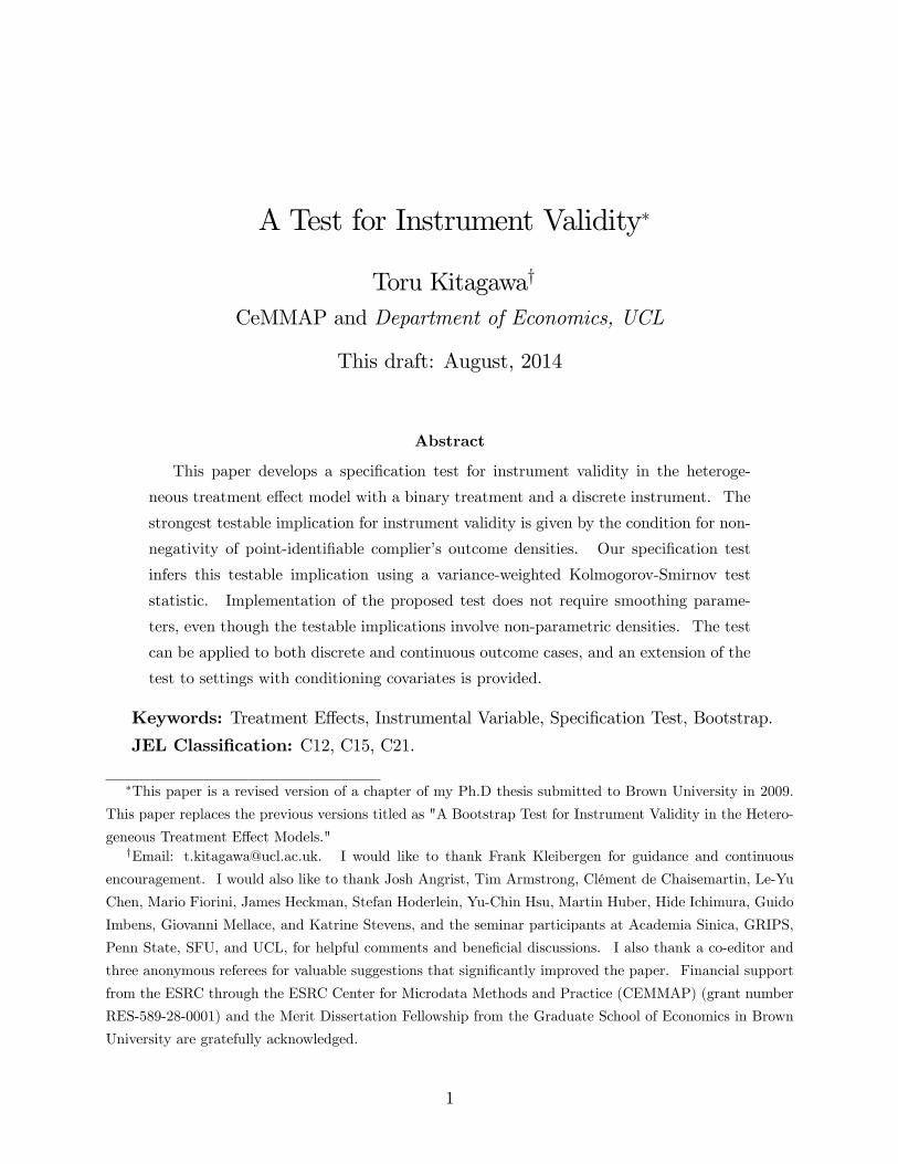
�This paper is a revised version of a chapter of my Ph.D thesis submitted to Brown University in 2009.

This paper replaces the previous versions titled as "A Bootstrap Test for Instrument Validity in the Hetero-

geneous Treatment E¤ect Models."yEmail: t.kitagawa@ucl.ac.uk. I would like to thank Frank Kleibergen for guidance and continuous

encouragement. I would also like to thank Josh Angrist, Tim Armstrong, Clément de Chaisemartin, Le-Yu

Chen, Mario Fiorini, James Heckman, Stefan Hoderlein, Yu-Chin Hsu, Martin Huber, Hide Ichimura, Guido

Imbens, Giovanni Mellace, and Katrine Stevens, and the seminar participants at Academia Sinica, GRIPS,

Penn State, SFU, and UCL, for helpful comments and bene�cial discussions. I also thank a co-editor and

three anonymous referees for valuable suggestions that signi�cantly improved the paper. Financial support

from the ESRC through the ESRC Center for Microdata Methods and Practice (CEMMAP) (grant number

RES-589-28-0001) and the Merit Dissertation Fellowship from the Graduate School of Economics in Brown

University are gratefully acknowledged.

1

1 Introduction

Consider a heterogeneous causal e¤ect model of Angrist and Imbens (1994) with a binary

treatment and a binary instrument. We denote an observed outcome by Y 2 Y � R, anobserved treatment status by D 2 f1; 0g; D = 1 when one receives the treatment while

D = 0 when one does not, and a binary non-degenerate instrument by Z 2 f1; 0g. Let

fYdz 2 Y : d 2 f1; 0g ; z 2 f1; 0gg be the potential outcomes that would have been observedif the treatment status were set at D = d and the assigned instrument were set at Z = z.

Furthermore, fDz : z 2 f1; 0gg are the potential treatment responses that would have beenobserved if Z = 1 and Z = 0, respectively. The seminal works of Imbens and Angrist

(1994) and Angrist, Imbens and Rubin (1996) showed that, given Pr(D = 1jZ = 1) >

Pr(D = 1jZ = 0), the instrument variable Z that satis�es the three conditions involving thepotential variables is able to identify the average treatment e¤ects for those whose selection

to treatment is a¤ected by the instrument (local average treatment e¤ect, LATE hereafter).

The three key conditions, of which the joint validity is hereafter referred to as IV-validity,

are1

Assumption: IV-validity for binary Z

1. Instrument Exclusion: Yd1 = Yd0 for d = 1; 0, with probability one.

2. Random Assignment: Z is jointly independent of (Y11; Y10; Y01; Y00; D1; D0).

3. Instrument Monotonicity (No-de�er): The potential participation indicators satisfy

D1 � D0 with probability one.

Despite the fact that the credibility of LATE analysis relies on the validity of the employed

instrument, no test procedure has been proposed to empirically diagnose IV-validity. As a

result, causal inference studies have assumed IV-validity based solely on some background

knowledge or out-of-sample evidence, and, accordingly, its credibility often remains contro-

versial in many empirical contexts.

The main contribution of this paper is to develop a speci�cation test for IV-validity in the

LATE model. Our speci�cation test builds on the testable implication obtained by Balke1Note that the null hypothesis of IV-validity tested in this paper does not include the instrument relevance

assumption, Pr(D = 1jZ = 1) > Pr(D = 1jZ = 0). The instrument relevance assumption can be assessedby inferring the coe¢ cient in the �rst-stage regression of D onto Z.

2

and Pearl (1997) and Heckman and Vytlacil (2005, Proposition A.5). Let P and Q be the

conditional probability distributions of (Y;D) 2 Y � f1; 0g given Z = 1 and Z = 0, i.e.,

P (B; d) = Pr(Y 2 B;D = djZ = 1);

Q(B; d) = Pr(Y 2 B;D = djZ = 0);

for Borel set B in Y and d = 1; 0. Imbens and Rubin (1997) showed that, under IV-validity,

P (B; 1)�Q(B; 1) = Pr(Y1 2 B;D1 > D0) and

Q(B; 0)� P (B; 0) = Pr(Y0 2 B;D1 > D0)

hold for every B in Y. Since the quantities in the right-hand sides are nonnegative by thede�nition of probabilities, we obtain the testable implication of Balke and Pearl (1997) and

Heckman and Vytlacil (2005);

P (B; 1)�Q(B; 1) � 0; (1.1)

Q(B; 0)� P (B; 0) � 0;

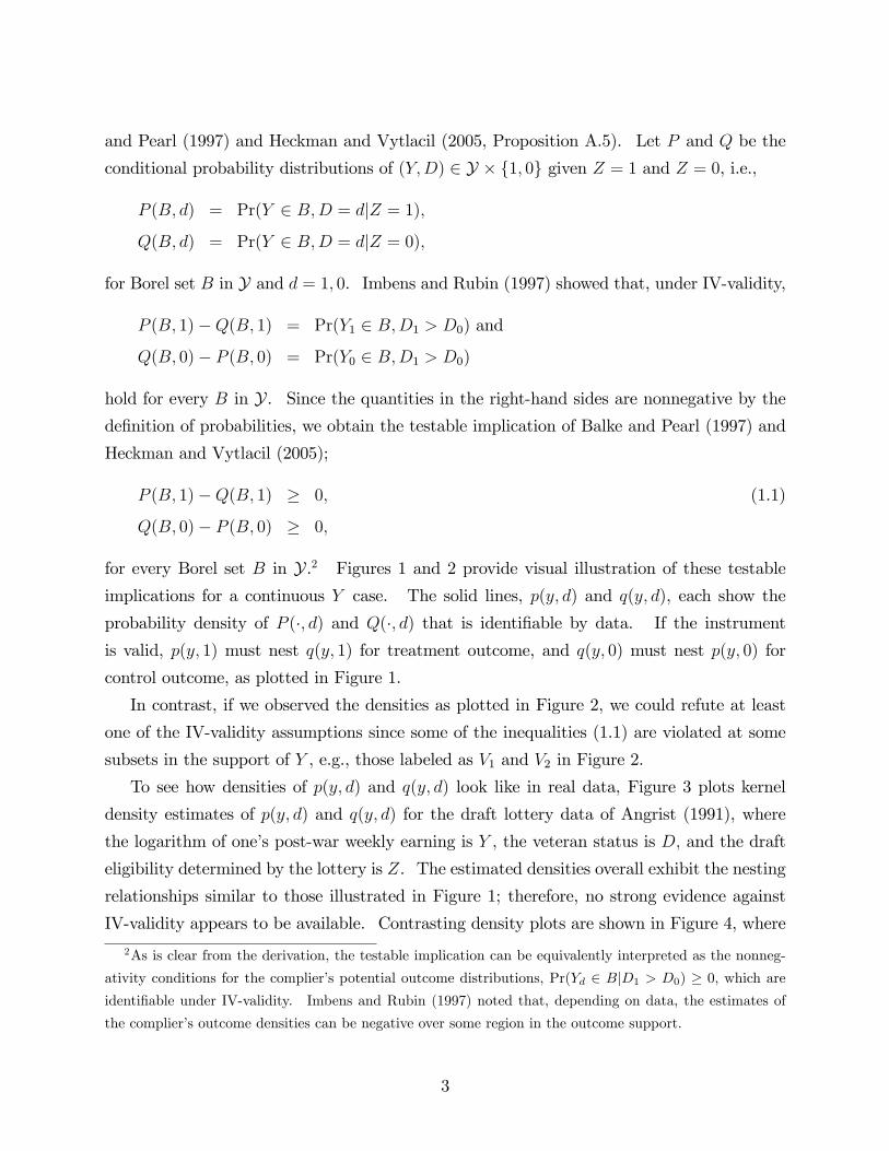
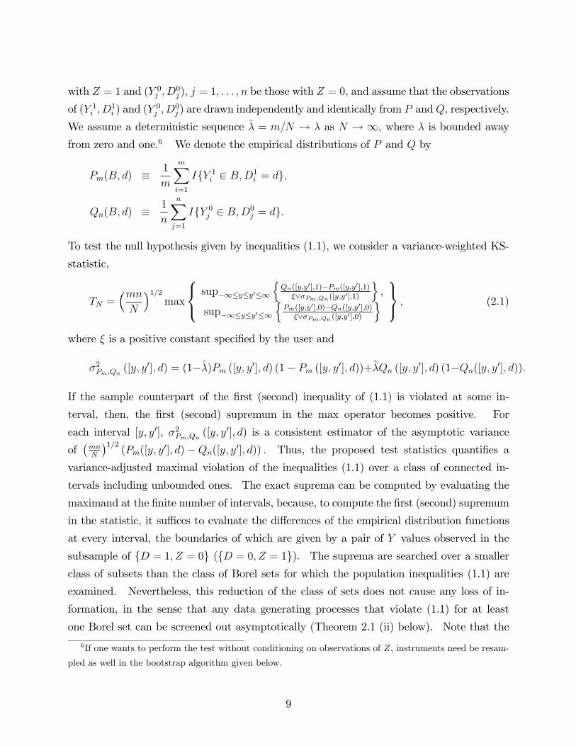
for every Borel set B in Y.2 Figures 1 and 2 provide visual illustration of these testable

implications for a continuous Y case. The solid lines, p(y; d) and q(y; d), each show the

probability density of P (�; d) and Q(�; d) that is identi�able by data. If the instrument

is valid, p(y; 1) must nest q(y; 1) for treatment outcome, and q(y; 0) must nest p(y; 0) for

control outcome, as plotted in Figure 1.

In contrast, if we observed the densities as plotted in Figure 2, we could refute at least

one of the IV-validity assumptions since some of the inequalities (1.1) are violated at some

subsets in the support of Y , e.g., those labeled as V1 and V2 in Figure 2.

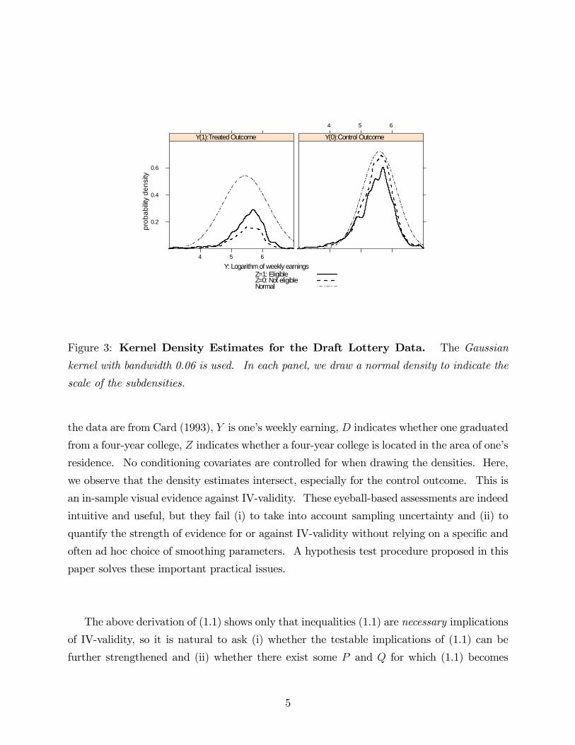
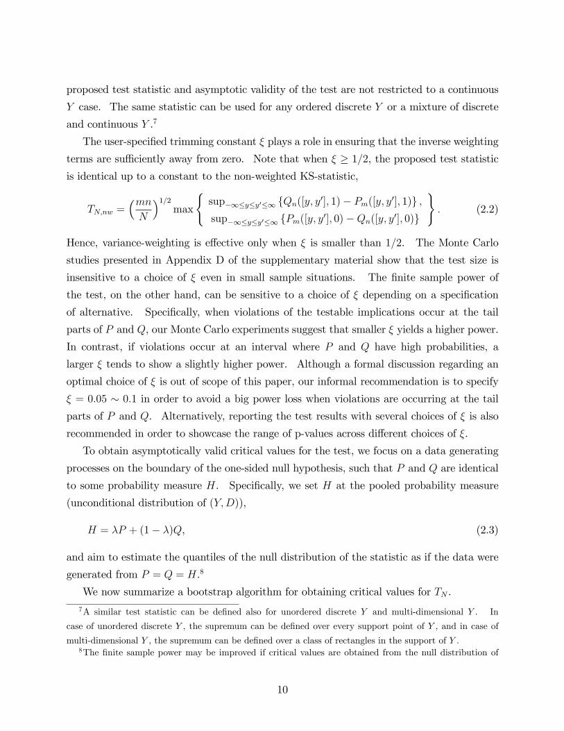
To see how densities of p(y; d) and q(y; d) look like in real data, Figure 3 plots kernel

density estimates of p(y; d) and q(y; d) for the draft lottery data of Angrist (1991), where

the logarithm of one�s post-war weekly earning is Y , the veteran status is D; and the draft

eligibility determined by the lottery is Z. The estimated densities overall exhibit the nesting

relationships similar to those illustrated in Figure 1; therefore, no strong evidence against

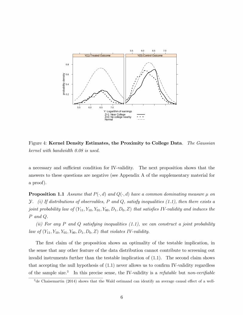
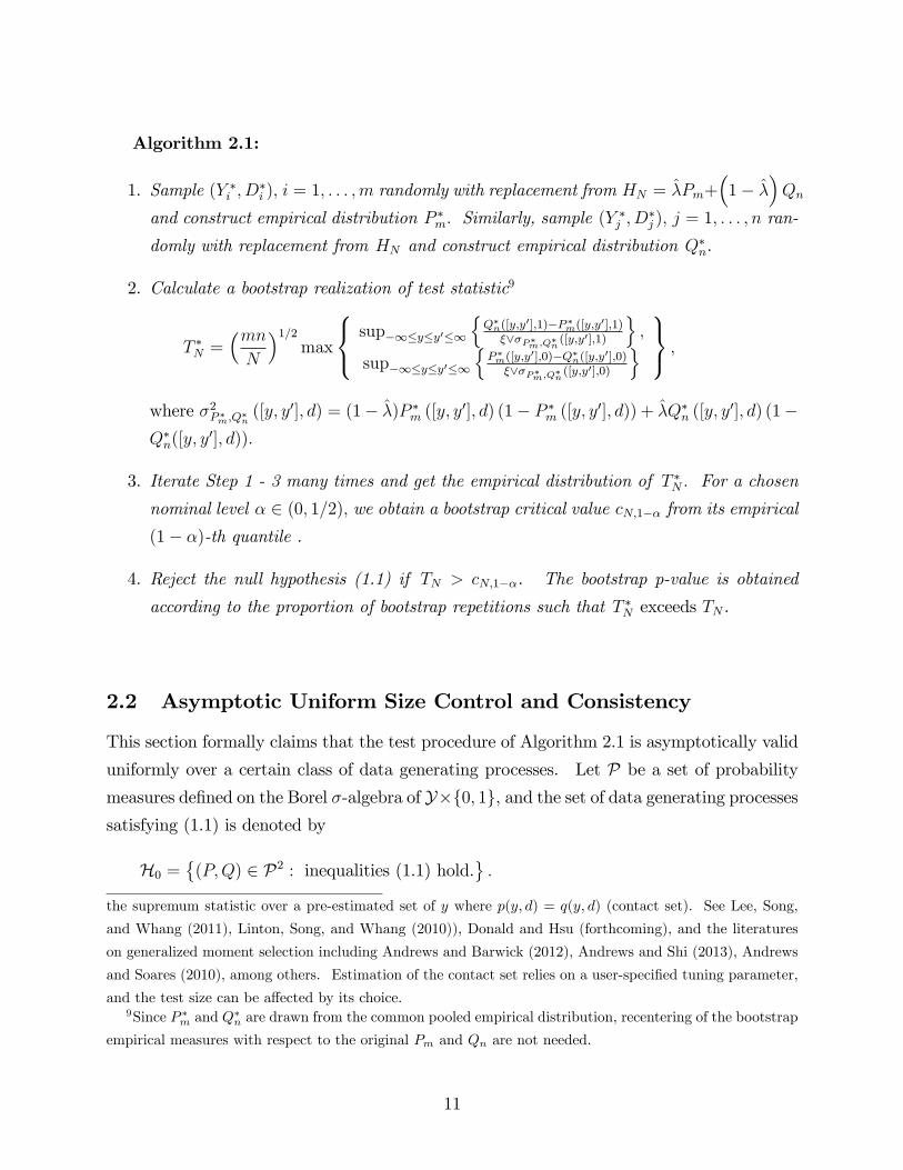
IV-validity appears to be available. Contrasting density plots are shown in Figure 4, where

2As is clear from the derivation, the testable implication can be equivalently interpreted as the nonneg-

ativity conditions for the complier�s potential outcome distributions, Pr(Yd 2 BjD1 > D0) � 0, which are

identi�able under IV-validity. Imbens and Rubin (1997) noted that, depending on data, the estimates of

the complier�s outcome densities can be negative over some region in the outcome support.

3

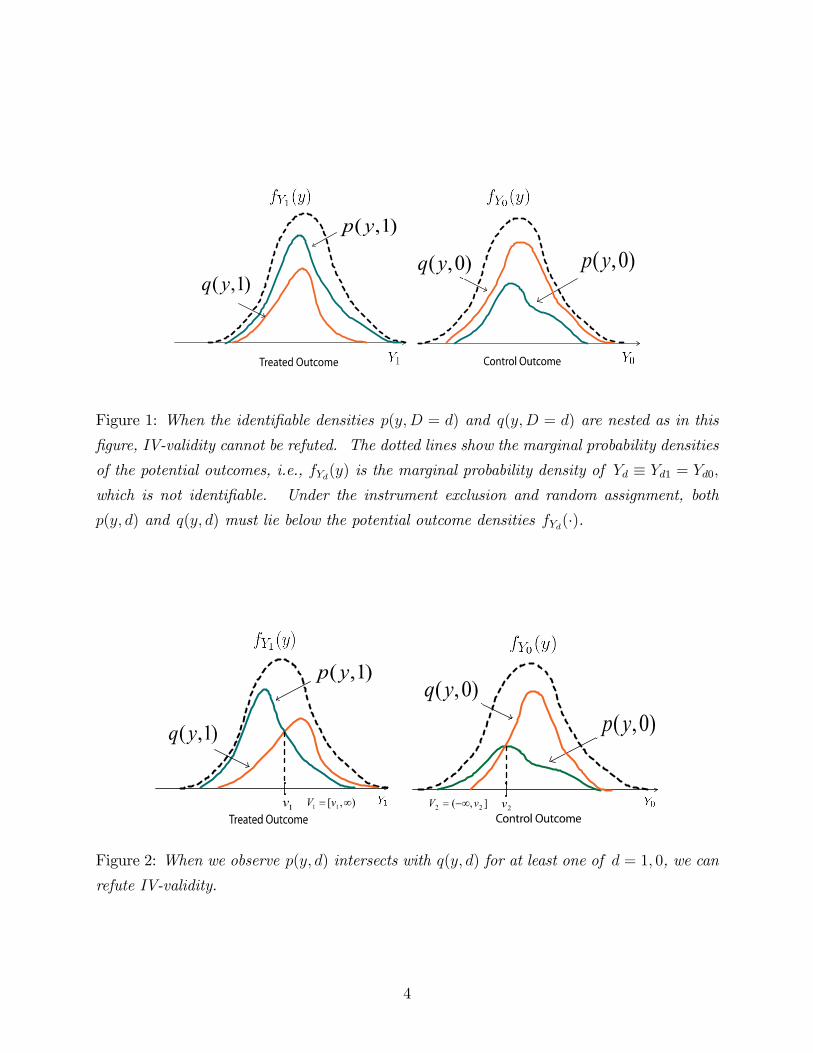
Figure 1: When the identi�able densities p(y;D = d) and q(y;D = d) are nested as in this

�gure, IV-validity cannot be refuted. The dotted lines show the marginal probability densities

of the potential outcomes, i.e., fYd(y) is the marginal probability density of Yd � Yd1 = Yd0;which is not identi�able. Under the instrument exclusion and random assignment, both

p(y; d) and q(y; d) must lie below the potential outcome densities fYd(�).

Figure 2: When we observe p(y; d) intersects with q(y; d) for at least one of d = 1; 0, we can

refute IV-validity.

4

Y: Logarithm of weekly earnings

prob

abilit

y de

nsity

0.2

0.4

0.6

4 5 6

Y(1):Treated Outcome4 5 6

Y(0):Control Outcome

Z=1: EligibleZ=0: Not eligibleNormal

Figure 3: Kernel Density Estimates for the Draft Lottery Data. The Gaussian

kernel with bandwidth 0.06 is used. In each panel, we draw a normal density to indicate the

scale of the subdensities.

the data are from Card (1993), Y is one�s weekly earning, D indicates whether one graduated

from a four-year college, Z indicates whether a four-year college is located in the area of one�s

residence. No conditioning covariates are controlled for when drawing the densities. Here,

we observe that the density estimates intersect, especially for the control outcome. This is

an in-sample visual evidence against IV-validity. These eyeball-based assessments are indeed

intuitive and useful, but they fail (i) to take into account sampling uncertainty and (ii) to

quantify the strength of evidence for or against IV-validity without relying on a speci�c and

often ad hoc choice of smoothing parameters. A hypothesis test procedure proposed in this

paper solves these important practical issues.

The above derivation of (1.1) shows only that inequalities (1.1) are necessary implications

of IV-validity, so it is natural to ask (i) whether the testable implications of (1.1) can be

further strengthened and (ii) whether there exist some P and Q for which (1.1) becomes

5

Y: Logarithm of earnings

prob

abilit

y de

nsity

0.2

0.4

0.6

0.8

5.5 6.0 6.5 7.0

Y(1):Treated Outcome

5.5 6.0 6.5 7.0

Y(0):Control Outcome

Z=1: Near CollegeZ=0: No college nearbyNormal

Figure 4: Kernel Density Estimates, the Proximity to College Data. The Gaussian

kernel with bandwidth 0.08 is used.

a necessary and su¢ cient condition for IV-validity. The next proposition shows that the

answers to these questions are negative (see Appendix A of the supplementary material for

a proof).

Proposition 1.1 Assume that P (�; d) and Q(�; d) have a common dominating measure � onY. (i) If distributions of observables, P and Q, satisfy inequalities (1.1), then there exists ajoint probability law of (Y11; Y10; Y01; Y00; D1; D0; Z) that satis�es IV-validity and induces the

P and Q.

(ii) For any P and Q satisfying inequalities (1.1), we can construct a joint probability

law of (Y11; Y10; Y01; Y00; D1; D0; Z) that violates IV-validity.

The �rst claim of the proposition shows an optimality of the testable implication, in

the sense that any other feature of the data distribution cannot contribute to screening out

invalid instruments further than the testable implication of (1.1). The second claim shows

that accepting the null hypothesis of (1.1) never allows us to con�rm IV-validity regardless

of the sample size.3 In this precise sense, the IV-validity is a refutable but non-veri�able3de Chaisemartin (2014) shows that the Wald estimand can identify an average causal e¤ect of a well-

6

hypothesis. Such limitation in terms of learnability of instrument validity is known in other

contexts, such as the classical over-identi�cation test in the linear instrumental variable

method with homogeneous e¤ect4 and the test of instrument monotonicity in the multi-

valued treatment case proposed in Angrist and Imbens (1995).5 See Breusch (1986) for a

general discussion on hypothesis testing of refutable but non-veri�able assumptions.

Our test uses a variance-weighted Kolmogorov-Smirnov test statistic (KS-statistic, here-

after) to measure the magnitude of violations of inequalities (1.1) in the data. We provide

a resampling algorithm to obtain critical values and demonstrate that the test procedure

attains asymptotically correct size uniformly over a large class of data generating processes,

and consistently rejects all the data generating processes violating (1.1). A similar variance

weighted KS-statistic has been considered in the literature of conditional moment inequal-

ities, as in Andrews and Shi (2013), Armstrong (2014), Armstrong and Chan (2013), and

Chetverikov (2012). As shown in Romano (1988), bootstrap is widely applicable and easy to

implement to obtain the critical values for general KS-statistic, and it has been instrumental

in the context of stochastic dominance testing; see, e.g., Abadie (2002), Barrett and Donald

(2003), Donald and Hsu (forthcoming), Horváth, Kokoszka, and Zitikis (2006), and Linton,

Maasoumi, and Whang (2005).

Our test concerns the exogeneity of instrument de�ned in terms of statistical indepen-

dence, and it can be applied to the context, in which objects of interest are distributional

features of complier�s potential outcome distribution, e.g., the quantile treatment e¤ects for

compliers (Abadie, Angrist, and Imbens (2002)). On the other hand, if solely the mean

de�ned subpopulation under the "Compliers-de�ers" assumption, which is weaker than the instrument

monotonicity assumption of Imbens and Angrist (1994). He shows that, even when instrument monotonicity

is replaced by the Complier-de�ners condition, the testable implication of (1.1) is a necessary, but is not an

if-and-only-if testable implication.4If the instrument is multi-valued, we can naively perform the classical over-identi�cation test by treating

the multi-valued instrument as a collection of binary instruments. However, as discussed in Imbens (2014)

and Lee (2014), the over-identi�cation test should not be used if causal e¤ects are considered to be heteroge-

neous, since heterogeneity of causal e¤ects can lead to misspeci�ed over-identifying restrictions, even when

LATE IV-validity is true.5In case of multi-valued treatment status, Angrist and Imbens (1995) propose a speci�cation test to assess

instrument monotonicity by inferring the stochastic dominance of the distribution functions of the treatment

status conditional on the instrument; see Barua and Lang (2009) and Fiorini, Stevens, Taylor, and Edwards

(2013) for applications of the Angrist and Imbens test. In the binary treatment case, however, Angrist and

Imbens test cannot be applied.

7

e¤ect is concerned, identi�cation of LATE can in fact be attained under a slightly weaker

set of assumptions, such that the instrument is statistically independent of the selection

types while the potential outcomes are only mean independent of Z conditional on each

selection type. Huber and Mellace (2013) show that this weaker LATE identifying condi-

tion has a testable implication given by a �nite number of moment inequalities. Since our

test builds on the distributional restrictions implied from statistical independence, it screens

out a larger class of data generating processes compared to the test of Huber and Mellace.

In addition, the set of detectable alternatives and the p-value of our test are invariant to

any monotonic transformation of the outcome variables, whereas this invariance property

does not hold for the Huber and Mellace�s test. Mouri�é and Wan (2014) recently consider

testing the same instrument validity condition as ours by applying the inference technique

developed by Chernozhukov, Lee, and Rosen (2013). Our test di¤ers from theirs at least

in the following three aspects. First, validity of their test assumes continuity of the density

of Y; which the LATE identi�cation and its consistent estimation do not require, whereas

our test does not require such continuity assumption. Second, in implementing their test,

one has to specify smoothing parameters, whereas our test is based solely on the empirical

distributions so its implementation is free from a choice of smoothing parameters. Third,

our test has nontrivial power against a class of nonparametric local alternatives shrinking to

null at N�1=2-rate, while, as shown in Chernozhukov et al (2013), the approach of Mouri�é

and Wan cannot attain nontrivial power against any nonparametric N�1=2-local alternatives.

The rest of the paper is organized as follows. Section 2 presents implementation of

our test when D and Z are binary and shows its asymptotic validity. Section 3 extends

the analysis to settings with a multi-valued instrument and with conditioning covariates.

Two empirical applications are provided in Section 4. The online supplementary material

provides proofs and results of Monte Carlo experiments.

2 Test

2.1 Test Statistics and Implementation

Let a sample be given by N observations of (Y;D;Z) 2 Y � f1; 0g2 : We divide the sampleinto two subsamples based on the value of Z, and we consider the sampling process as being

conditional on a sequence of instrument values. Let (Y 1i ; D1i ); i = 1; : : : ;m be observations

8

with Z = 1 and (Y 0j ; D0j ); j = 1; : : : ; n be those with Z = 0, and assume that the observations

of (Y 1i ; D1i ) and (Y

0j ; D

0j ) are drawn independently and identically from P andQ, respectively.

We assume a deterministic sequence �̂ = m=N ! � as N ! 1, where � is bounded awayfrom zero and one.6 We denote the empirical distributions of P and Q by

Pm(B; d) � 1

m

mXi=1

IfY 1i 2 B;D1i = dg;

Qn(B; d) � 1

n

nXj=1

IfY 0j 2 B;D0j = dg:

To test the null hypothesis given by inequalities (1.1), we consider a variance-weighted KS-

statistic,

TN =�mnN

�1=2max

8<: sup�1�y�y0�1

nQn([y;y0];1)�Pm([y;y0];1)�_�Pm;Qn ([y;y

0];1)

o;

sup�1�y�y0�1

nPm([y;y0];0)�Qn([y;y0];0)�_�Pm;Qn ([y;y

0];0)

o 9=; ; (2.1)

where � is a positive constant speci�ed by the user and

�2Pm;Qn ([y; y0]; d) = (1��̂)Pm ([y; y0]; d) (1� Pm ([y; y0]; d))+�̂Qn ([y; y0]; d) (1�Qn([y; y0]; d)):

If the sample counterpart of the �rst (second) inequality of (1.1) is violated at some in-

terval, then, the �rst (second) supremum in the max operator becomes positive. For

each interval [y; y0], �2Pm;Qn ([y; y0]; d) is a consistent estimator of the asymptotic variance

of�mnN

�1=2(Pm([y; y

0]; d)�Qn([y; y0]; d)) : Thus, the proposed test statistics quanti�es a

variance-adjusted maximal violation of the inequalities (1.1) over a class of connected in-

tervals including unbounded ones. The exact suprema can be computed by evaluating the

maximand at the �nite number of intervals, because, to compute the �rst (second) supremum

in the statistic, it su¢ ces to evaluate the di¤erences of the empirical distribution functions

at every interval, the boundaries of which are given by a pair of Y values observed in the

subsample of fD = 1; Z = 0g (fD = 0; Z = 1g). The suprema are searched over a smaller

class of subsets than the class of Borel sets for which the population inequalities (1.1) are

examined. Nevertheless, this reduction of the class of sets does not cause any loss of in-

formation, in the sense that any data generating processes that violate (1.1) for at least

one Borel set can be screened out asymptotically (Theorem 2.1 (ii) below). Note that the

6If one wants to perform the test without conditioning on observations of Z, instruments need be resam-

pled as well in the bootstrap algorithm given below.

9

proposed test statistic and asymptotic validity of the test are not restricted to a continuous

Y case. The same statistic can be used for any ordered discrete Y or a mixture of discrete

and continuous Y .7

The user-speci�ed trimming constant � plays a role in ensuring that the inverse weighting

terms are su¢ ciently away from zero. Note that when � � 1=2, the proposed test statisticis identical up to a constant to the non-weighted KS-statistic,

TN;nw =�mnN

�1=2max

(sup�1�y�y0�1 fQn([y; y0]; 1)� Pm([y; y0]; 1)g ;sup�1�y�y0�1 fPm([y; y0]; 0)�Qn([y; y0]; 0)g

): (2.2)

Hence, variance-weighting is e¤ective only when � is smaller than 1=2. The Monte Carlo

studies presented in Appendix D of the supplementary material show that the test size is

insensitive to a choice of � even in small sample situations. The �nite sample power of

the test, on the other hand, can be sensitive to a choice of � depending on a speci�cation

of alternative. Speci�cally, when violations of the testable implications occur at the tail

parts of P and Q, our Monte Carlo experiments suggest that smaller � yields a higher power.

In contrast, if violations occur at an interval where P and Q have high probabilities, a

larger � tends to show a slightly higher power. Although a formal discussion regarding an

optimal choice of � is out of scope of this paper, our informal recommendation is to specify

� = 0:05 � 0:1 in order to avoid a big power loss when violations are occurring at the tailparts of P and Q. Alternatively, reporting the test results with several choices of � is also

recommended in order to showcase the range of p-values across di¤erent choices of �.

To obtain asymptotically valid critical values for the test, we focus on a data generating

processes on the boundary of the one-sided null hypothesis, such that P and Q are identical

to some probability measure H. Speci�cally, we set H at the pooled probability measure

(unconditional distribution of (Y;D)),

H = �P + (1� �)Q, (2.3)

and aim to estimate the quantiles of the null distribution of the statistic as if the data were

generated from P = Q = H.8

We now summarize a bootstrap algorithm for obtaining critical values for TN .

7A similar test statistic can be de�ned also for unordered discrete Y and multi-dimensional Y . In

case of unordered discrete Y , the supremum can be de�ned over every support point of Y , and in case of

multi-dimensional Y , the supremum can be de�ned over a class of rectangles in the support of Y .8The �nite sample power may be improved if critical values are obtained from the null distribution of

10

Algorithm 2.1:

1. Sample (Y �i ; D�i ); i = 1; : : : ;m randomly with replacement from HN = �̂Pm+

�1� �̂

�Qn

and construct empirical distribution P �m: Similarly, sample (Y�j ; D

�j ); j = 1; : : : ; n ran-

domly with replacement from HN and construct empirical distribution Q�n.

2. Calculate a bootstrap realization of test statistic9

T �N =�mnN

�1=2max

8<: sup�1�y�y0�1

nQ�n([y;y

0];1)�P �m([y;y0];1)�_�P�m;Q�n ([y;y

0];1)

o;

sup�1�y�y0�1

nP �m([y;y

0];0)�Q�n([y;y0];0)�_�P�m;Q�n ([y;y

0];0)

o 9=; ;where �2P �m;Q�n ([y; y

0]; d) = (1� �̂)P �m ([y; y0]; d) (1� P �m ([y; y0]; d)) + �̂Q�n ([y; y0]; d) (1�Q�n([y; y

0]; d)):

3. Iterate Step 1 - 3 many times and get the empirical distribution of T �N : For a chosen

nominal level � 2 (0; 1=2); we obtain a bootstrap critical value cN;1�� from its empirical(1� �)-th quantile .

4. Reject the null hypothesis (1.1) if TN > cN;1��. The bootstrap p-value is obtained

according to the proportion of bootstrap repetitions such that T �N exceeds TN .

2.2 Asymptotic Uniform Size Control and Consistency

This section formally claims that the test procedure of Algorithm 2.1 is asymptotically valid

uniformly over a certain class of data generating processes. Let P be a set of probability

measures de�ned on the Borel �-algebra of Y�f0; 1g, and the set of data generating processessatisfying (1.1) is denoted by

H0 =�(P;Q) 2 P2 : inequalities (1.1) hold.

:

the supremum statistic over a pre-estimated set of y where p(y; d) = q(y; d) (contact set). See Lee, Song,

and Whang (2011), Linton, Song, and Whang (2010)), Donald and Hsu (forthcoming), and the literatures

on generalized moment selection including Andrews and Barwick (2012), Andrews and Shi (2013), Andrews

and Soares (2010), among others. Estimation of the contact set relies on a user-speci�ed tuning parameter,

and the test size can be a¤ected by its choice.9Since P �m and Q

�n are drawn from the common pooled empirical distribution, recentering of the bootstrap

empirical measures with respect to the original Pm and Qn are not needed.

11

The uniform validity of our test procedure is based on the following two weak regularity

conditions.

Condition-RG:

(a) Probability measures in P are nondegenerate and have a common dominating measure

� for the Y-coordinate, where � is the Lebesgue measure, a point mass measure with �nitesupport points, or their mixture. The density functions p(y; d) � dP (�;d)

d�are bounded

uniformly over P, i.e., there exists M < 1 such that p(y; d) � M holds at �-almost every

y 2 Y and d = 0; 1 for all P 2 P.(b) P is uniformly tight, i.e., for arbitrary � > 0, there exists a compact set K � Y�f0; 1gsuch that

supP2P

fP (Kc)g < �.

The asymptotic validity of the proposed test is stated in the next proposition (see Ap-

pendix B of the supplementary material for a proof).

Theorem 2.1 Suppose Condition-RG. Let � 2 (0; 1=2). (i) The test procedure of Algo-

rithm 2.1 has asymptotically uniformly correct size for null hypothesis H0,

lim supN!1

sup(P;Q)2H0

Pr (TN > cN;1��) � �:

(ii) For a �xed data generating process that violates inequalities (1.1) for some Borel set B,

the test based on TN is consistent, i.e., the rejection probability converges to one as N !1.

This theorem establishes asymptotic uniform validity of the proposed test procedure over

P. The second claim of the proposition concerns the power of the test, and it shows that

any �xed alternative within P can be consistently rejected.

2.3 Power against N�1=2-local Alternatives

In this section, we show that the proposed test has nontrivial power against a class of

non-parametric N�1=2-local alternatives. Let��P [N ]; Q[N ]

�2 P2 : N = 1; 2; : : :

denote a

sequence of probability measures on Y � f1; 0g shrinking to (P0; Q0) 2 H0. The next

assumption de�nes a class of local alternatives, against which we derive power of our test.

12

Assumption-LA:

A sequence of true alternatives��P [N ]; Q[N ]

�2 P2 : N = 1; 2; : : :

is represented by

P [N ] = P0 +N�1=2�

[N ]1 and (2.4)

Q[N ] = Q0 +N�1=2�

[N ]0 ;

where (P0; Q0) 2 P2 is a pair of probability measures on Y�f1; 0g andn��[N ]1 ; �

[N ]0

�: N = 1; 2; : : :

ois a sequence of bounded signed measures on Y � f1; 0g.(a) (P0; Q0) 2 H0 and P0 ([y; y0] ; d) = Q0 ([y; y

0] ; d) > 0 for some �1 � y � y0 � 1,and d 2 f1; 0g.(b) For all N , �N1=2P0 � �

[N ]1 < 1 and �N1=2Q0 � �

[N ]0 < 1 hold and �[N ]1 (Y ; d) =

�[N ]0 (Y ; d) = 0 for d = 1; 0.(c) �[N ]1 � �[N ]0 converges in terms of the sup metric over Borel sets to a bounded signed

measure �� as N !1.(d) For some ([y; y0] ; d) satisfying (a), �� ([y; y0] ; 1) < 0 and/or �� ([y; y0] ; 0) > 0 hold.

Assumption-LA (a) says that (P0; Q0) 2 H0; to which�P [N ]; Q[N ]

�converges, has a

nonempty contact set with a positive measure in terms of P0 = Q0. Assumption-LA (b)

ensures�P [N ]; Q[N ]

�2 P2 and Pr(D = 1jZ = 1) � Pr(D = 1jZ = 0) for all N , and P [N ] and

Q[N ] are in an N�1=2-neighborhood of P0 and Q0 in terms of the total variation distance.

Assumption-LA (c) implies thatpN�P [N ] �Q[N ]

�([y; y0] ; d)! �� ([y; y0] ; d) at every [y; y0]

contained in the contact set of P0 and Q0. Accordingly, combined with Assumption-LA (d),�P [N ]; Q[N ]

�violates the IV-validity testable implication at some [y; y0] contained in the

contact set for all large N .

The next theorem provides a lower bound of the power of our test along N�1=2-local

alternatives satisfying Assumption-LA.

Theorem 2.2 Assume Condition-RG and��P [N ]; Q[N ]

�2 P2 : N = 1; 2; : : :

satis�es Assumption-

LA. Then,

limN!1

PrP [N ];Q[N ]

(TN > cN;1��) � 1� �(t);

where �(�) is the cumulative distribution function of the standard normal distribution,

t =

��2P0;Q0 ([y; y

0] ; 1)

�2^ 1��1 �

c1�� � [�(1� �)]1=2j�� ([y; y0] ; d)j

� _ �P0;Q0 ([y; y0] ; 1)

�;

13

c1�� is the limit of the bootstrap critical value of Algorithm 2.1 that is bounded and depends

only on (�; �; �; P0; Q0), and ([y; y0] ; d) is as de�ned in Assumption-LA (a) and (d).

Note that the provided lower bound of the power is increasing in j�� ([y; y0] ; d)j and itapproaches one as a deviation from the null j�� ([y; y0] ; d)j gets larger. Hence, we concludethat, for some N�1=2-local alternatives satisfying Assumption-LA, the power is greater than

the size of the test for every � 2 (0; 1=2).

3 Extensions

3.1 A Multi-valued Discrete Instrument

The test procedure proposed above can be extended straightforwardly to a case with a

multi-valued discrete instrument, Z 2 fz1; z2; : : : ; zKg. Let p(zk) = Pr(D = 1jZ = zk),

and assume knowledge of the ordering of p(zk), so that without loss of generality we assume

p(z1) � � � � � p(zK). With the multi-valued instrument, we denote the potential outcomesindexed by treatment and instrument status by fYdz : d = 0; 1; z = z1; : : : ; zKg, and potentialselection responses by fDz : z = z1; : : : ; zKg : The following assumptions guarantee that thelinear two-stage least squares estimator can be interpreted as a weighted averages of the

compliers average treatment e¤ects (Imbens and Angrist (1994)).

Assumption: IV-validity for Multi-valued Discrete Z

1. Instrument Exclusion: Ydz1 = Ydz2 = � � � = YdzK for d = 1; 0, with probability one.

2. Random Assignment: Z is jointly independent of (Y1z1 ; : : : ; Y1zK ; Y0z1 ; : : : ; Y0zK ) and

(Dz1 ; : : : ; DzK ).

3. Instrument Monotonicity: Given p(z1) � � � � � p(zK), the potential selection indica-tors satisfy Dzk+1 � Dzk with probability one for every k = 1; : : : ; (K � 1).

Let P (B; djzk) = Pr(Y 2 B;D = djZ = zk), k = 1; : : : ; K, and Pmk(B; djzk) be its empir-

ical distribution based on the subsample of Zi = zk with size mk. The testable implication

of the binary instrument case is now generalized to the following set of inequalities,

P (B; 1jz1) � P (B; 1jz2) � � � � � P (B; 1jzK) and

P (B; 0jz1) � P (B; 0jz2) � � � � � P (B; 0jzK)(3.1)

14

for all Borel set B in Y. Using the test statistic for the binary Z case to measure the

violation of the inequalities across the neighboring values of Z, we can develop a statistic

that jointly tests the inequalities of (3.1),

TN = max fTN;1; : : : ; TN;K�1g ; (3.2)

where, for k = 1; : : : ; (K � 1);

TN;k =

�mkmk+1

mk +mk+1

�1=2max

8<: sup�1�y�y0�1

nPmk ([y;y

0];1jzk)�Pmk+1 ([y;y0];1jzk+1)

�k_�k([y;y0];1)

o;

sup�1�y�y0�1

nPmk+1 ([y;y

0];0jzk+1)�Pmk ([y;y0];0jzk)

�k_�k([y;y0];0)

o 9=; ;�2k ([y; y

0]; d) =

�mk+1

mk +mk+1

�Pmk

([y; y0]; djzk) (1� Pmk([y; y0]; djzk))

+

�mk

mk +mk+1

�Pmk+1

([y; y0]; djzk)(1� Pmk+1([y; y0]; djzk));

and �1; : : : ; �K�1 are positive constants. Critical values can be obtained by applying a

resampling algorithm of the previous section to each TN;k simultaneously.

Algorithm 3.1:

1. LetHN;k (�) =�

mk+1

mk+mk+1

�Pmk+1

(�jzk+1)+�

mk

mk+mk+1

�Pmk

(�jzk) be the pooled empiricalmeasures that pool the sample of Zi = zk+1 and that of Zi = zk. Sample (Y �i ; D

�i ); i =

1; : : : ;mk+1 randomly with replacement from HN;k and construct the bootstrap empirical

distribution P �mk+1(�jzk+1): Similarly, sample (Y �j ; D�

j ); j = 1; : : : ;mk randomly with

replacement from HN;k and construct the bootstrap empirical distribution P �mk(�jzk):

2. Apply step 1 for every k = 1; : : : ; (K � 1), and obtain (K � 1) pairs of the re-sampled empirical measures, (P �m1

; P �m2), (P �m2

; P �m3); : : : ; (P �mK�1

; P �mK). De�ne, for

k = 1; : : : ; (K � 1);

��2k ([y; y0]; d) =

�mk+1

mk +mk+1

�P �mk

([y; y0]; djzk)�1� P �mk

([y; y0]; djzk)�

+

�mk

mk +mk+1

�P �mk+1

([y; y0]; djzk+1)(1� P �mk+1([y; y0]; djzk+1));

T �N;k =

�mkmk+1

mk +mk+1

�1=2�max

8<: sup�1�y�y0�1

nP �mk ([y;y

0];1jzk)�P �mk+1 ([y;y0];1jzk+1)

�k_��k([y;y0];1)

o;

sup�1�y�y0�1

nP �mk+1 ([y;y

0];0jzk+1)�P �mk ([y;y0];0jzk)

�k_��k([y;y0];0)

o9=; ;

15

where �k, k = 1; : : : ; (K � 1), are positive constants. The bootstrap statistic T �N is

computed accordingly by T �N = max�T �N;1; : : : ; T

�N;K�1

.

3. Iterate Step 1 -3 many times, get the empirical distribution of T �N , and obtain a boot-

strap critical value cN;1�� from its empirical (1� �)-th quantile .

4. Reject the null hypothesis (3.1) if TN > cN;1��. The bootstrap p-value is obtained by

the proportion of T �N�s greater than TN .

3.2 Conditioning Covariates

Empirical studies commonly use observable conditioning covariates in the context of instru-

mental variable methods. One of the major motivations for introducing them is to control

for potential confounders that invalidate the random assignment assumption. This section

brie�y discusses how to extend IV-validity test proposed above to the settings with condi-

tioning covariates, X 2 X�Rdx, used for this purpose.IV-validity to be tested in this case consists of the joint restriction of instrument exclusion,

instrument monotonicity, and the conditional version of the instrument random assignment

assumption, (Y11; Y10; Y01; Y00; D1; D0) ? ZjX. These three assumptions combined with

the �rst stage rank condition, Pr(D = 1jZ = 1; X) 6= Pr(D = 1jZ = 0; X) for some X,

guarantees that the linear two stage least squares with a function of (Z;X) used as an

instrument (e.g. Pr(D = 1jZ;X)) estimates a certain weighted average of the complier�sconditional causal e¤ects E(Y1 � Y0jT = c;X) (Heckman and Vytlacil (2005)). Moreover,

under the same set of assumptions, the semiparametric IV estimator developed by Abadie

(2003) consistently estimates the unconditional complier�s causal e¤ect E(Y1 � Y0jT = c).A testable implication with the largest screening power in the sense similar to Proposition

1.1 is given by the conditional version of the inequalities (1.1), i.e., for every Borel set B � Yand X 2 X,

Pr(Y 2 B;D = 1jZ = 1; X)� Pr(Y 2 B;D = 1jZ = 0; X) � 0; (3.3)

Pr(Y 2 B;D = 0jZ = 0; X)� Pr(Y 2 B;D = 0jZ = 1; X) � 0:

As shown in Lemma B.8 in the supplementary material, the use of Theorem 3.1 of Abadie

(2003) and the instrument function argument for conditional moment inequalities as given

in Andrews and Shi (2013) and Khan and Tamer (2009) enable us to reduce (3.3) to the

16

following unconditional moment inequalities without loss of any information,10

E [�1 (D;Z;X) g(Y;X)] � 0; (3.4)

E [�0 (D;Z;X) g(Y;X)] � 0; for all g(�; �) 2 G

where

�1 (D;Z;X) = DZ � Pr(Z = 1jX)

Pr(Z = 0jX) Pr(Z = 1jX) ;

�0 (D;Z;X) = (1�D) (1� Z)� Pr(Z = 0jX)Pr(Z = 0jX) Pr(Z = 1jX) ;

and G is the class of indicator functions for boxes in Y � X ,

G =(1 f(Y;X) 2 Cg : C = [y; y0]� [x1; x01]� � � � �

�xdx ; x

0dx

�, �1 � y � y0 � 1 ,

�1 � xl � x0l � 1; l = 1; : : : ; dx.

):

(3.5)

Accordingly, a variance-weighted KS statistic to infer (3.4) can be proposed as

TN =pN max

(supg2G

�EN [�̂1(D;Z;X)g(Y;X)]�_�̂1(g) ;

supg2G�EN [�̂0(D;Z;X)g(Y;X)]

�_�̂0(g)

);

where �̂d is an estimate of �d with estimated Pr(Z = 1jX) plugged in, EN (�) is the sampleaverage, and �̂2d (g) is the sample variance of �̂d (Di; Zi; Xi) g(Yi; Xi). Ignoring estimation

uncertainty of �̂d; the critical values can be obtained by bootstrapping the supremum statistic

of the recentered moments,

T �N =pN max

8<: supg2G�[E�N [�̂1(D;Z;X)g(Y;X)]�EN [�̂1(D;Z;X)g(Y;X)]]

�_�̂�1(g);

supg2G�[E�N [�̂0(D;Z;X)g(Y;X)]�EN [�̂0(D;Z;X)g(Y;X)]]

�_�̂�0(g)

9=; ;where E�N (�) is the sample average based on a bootstrap sample that is obtained by resam-pling (Y;D;Z;X) from the original sample, and �̂�2d (g) is the variance estimate based on the

bootstrap sample.10If the random assignment assumption is strengthened to (Y11; Y10; Y01; Y00; D1; D0; X) ? Z, then it can

be shown that the moment conditions of (3.4) are reduced to

Pr((Y;X) 2 C;D = 1jZ = 1)� Pr((Y;X) 2 C;D = 1jZ = 0) � 0;

Pr((Y;X) 2 C;D = 0jZ = 0)� Pr((Y;X) 2 C;D = 0jZ = 1) � 0;

for any box C in Y�X . As a result, the test procedure for no-covariate case can be extended straightforwardlyto this case.

17

Regarding implementations of this procedure in practice, a couple of issues need to be

addressed. First, in the presence of many covariates, computation of the statistic involves an

optimization over a large class of indicator functions. This raises a computational di¢ culty in

implementing the test. Second, the proposed approach requires estimation of Pr(Z = 1jX),which the linear two stage least squares estimation do not require. Hence, if a parametric

estimation for Pr(Z = 1jX) is used to implement the test, the validity of the test relies onthe assumption of a correct functional form for Pr(Z = 1jX), and rejection can be driven byits misspeci�cation rather than the violation of IV-validity.

4 Empirical Applications

We illustrate a use of our test using the two data sets mentioned in Introduction.

4.1 Draft Lottery Data

The draft lottery data of Angrist (1991) consist of a sample of 10,101 white men, born

between 1950 and 1953 extracted from March Current Population Surveys of 1979 and 1981-

1985. The outcome variable is measured in terms of the logarithm of weekly earnings

imputed by the annual labor earnings divided by weeks worked. The treatment is whether

one has a Vietnam veteran status. In order to cope with the selection to treatment status,

Angrist (1991) constructed the binary indicator of the draft eligibility, which is randomly

assigned based on one�s birthdate through the draft lotteries. It is reasonable to believe that

the constructed instrument is independent of any individual characteristics, and de�ers do

not exist in the population even though the sampling design does not exclude the possibility

of having them. A less credible assumption in the current context would be instrument

exclusion. For instance, the draft lottery can directly a¤ect control outcomes for some

never-takers if those who were drafted change their career choice, school years, or migration

choice for the purpose of escaping from the military service.

Table 1 shows the result of our test. We present the bootstrap p-values of our test for

several di¤erent speci�cations of the trimming constant. All of them are one, so we do not

reject validity of the draft lottery instrument from the data.

18

4.2 Returns to Education: Proximity to College Data

The Card data is based on National Longitudinal Survey of Young Men (NLSYM) that began

in 1966 with 14-24 years old men and continued with follow-up surveys through 1981. Based

on the respondents�county of residence at 1966, the Card data provides the presence of a

4-year college in the local labor market. The observations of years of education and wages

were based on the follow-ups�educational attainment and wages reported in the interview

in 1976.

Proximity to college was used as an instrument, because the presence of a nearby college

reduces the cost of college education by allowing students to live at their home, while one�s

unobservable ability is presumably independent of student�s residence during their teenage

years. Compliers in this context can be considered as those who grew up in relatively low-

income families and who were not able to go to college without living with their parents.

Being di¤erent from the original Card�s study, we treat the educational level as a binary

treatment, with years of education greater than or equal to 16 years, that is, the treatment

can be considered as a four year college degree.

We specify the measure of outcome to be the logarithm of weekly earnings. In the

�rst speci�cation, we do not control for any demographic covariates. This raises a concern

regarding the violation of random assignment assumption. For instance, one�s region of

residence, or whether they were born in the standard metropolitan area or rural area. may

well be dependent on one�s wage levels and the proximity to colleges if the urban areas are

more likely to have colleges and higher wage levels compared to the rural areas.

Our test procedure yields zero p-values for each choice of trimming constant. This pro-

vides an empirical evidence that, without controlling for any covariates, college proximity is

not a valid instrument.

19

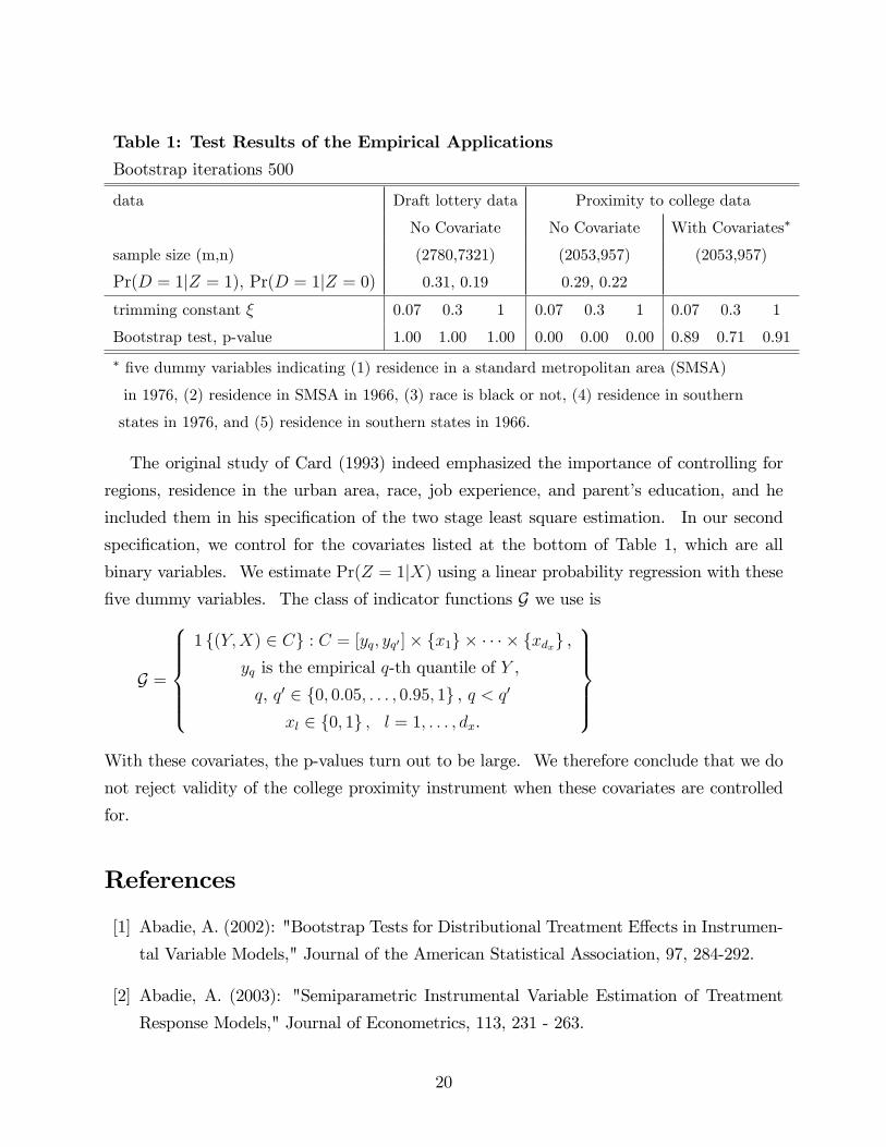
Table 1: Test Results of the Empirical Applications

Bootstrap iterations 500

data Draft lottery data Proximity to college data

No Covariate No Covariate With Covariates�

sample size (m,n) (2780,7321) (2053,957) (2053,957)

Pr(D = 1jZ = 1); Pr(D = 1jZ = 0) 0.31, 0.19 0.29, 0.22

trimming constant � 0.07 0.3 1 0.07 0.3 1 0.07 0.3 1

Bootstrap test, p-value 1.00 1.00 1.00 0.00 0.00 0.00 0.89 0.71 0.91

� �ve dummy variables indicating (1) residence in a standard metropolitan area (SMSA)

in 1976, (2) residence in SMSA in 1966, (3) race is black or not, (4) residence in southern

states in 1976, and (5) residence in southern states in 1966.

The original study of Card (1993) indeed emphasized the importance of controlling for

regions, residence in the urban area, race, job experience, and parent�s education, and he

included them in his speci�cation of the two stage least square estimation. In our second

speci�cation, we control for the covariates listed at the bottom of Table 1, which are all

binary variables. We estimate Pr(Z = 1jX) using a linear probability regression with these�ve dummy variables. The class of indicator functions G we use is

G =

8>>>><>>>>:1 f(Y;X) 2 Cg : C = [yq; yq0 ]� fx1g � � � � � fxdxg ,

yq is the empirical q-th quantile of Y ,

q, q0 2 f0; 0:05; : : : ; 0:95; 1g , q < q0

xl 2 f0; 1g ; l = 1; : : : ; dx.

9>>>>=>>>>;With these covariates, the p-values turn out to be large. We therefore conclude that we do

not reject validity of the college proximity instrument when these covariates are controlled

for.

References

[1] Abadie, A. (2002): "Bootstrap Tests for Distributional Treatment E¤ects in Instrumen-

tal Variable Models," Journal of the American Statistical Association, 97, 284-292.

[2] Abadie, A. (2003): "Semiparametric Instrumental Variable Estimation of Treatment

Response Models," Journal of Econometrics, 113, 231 - 263.

20

[3] Abadie, A., J. D. Angrist, and G. W. Imbens. (2002): "Instrumental Variables Es-

timates of the E¤ect of Subsidized Training on the Quantiles of Trainee Earnings,"

Econometrica, 70, 91-117.

[4] Andrews, D.W.K. and P. Jia Barwick (2012): "Inference for Parameters De�ned by

Moment Inequalities: A Recommended Moment Selection Procedure," Econometrica,

80, 2805-2826.

[5] Andrews, D.W.K. and X. Shi (2013): "Inference Based on Conditional Moment Inequal-

ities," Econometrica, 81, 609-666.

[6] Andrews, D.W.K. and G. Soares (2010): "Inference for Parameters De�ned by Moment

Inequalities Using Generalized Moment Selection," Econometrica, 78, 119-157.

[7] Angrist, J. D. (1991): "The Draft Lottery and Voluntary Enlistment in the Vietnam

Era," Journal of the American Statistical Association, 86, 584-595

[8] Angrist, J.D., G.W. Imbens (1995): "Two-stage Least Squares Estimation of Aver-

age Causal E¤ects Using Instrumental Variables," Journal of the American Statistical

Association, 91, 444-455.

[9] Angrist, J. D., G. W. Imbens, and D. B. Rubin (1996): "Identi�cation of Causal E¤ects

Using Instrumental Variables," Journal of the American Statistical Association, 91,

444-455.

[10] Armstrong, T.B. and H.P. Chan (2013): "Multiscale Adaptive Inference on Conditional

Moment Inequalities," Cowles Foundation Discussion Paper, No. 1885. Yale University.

[11] Armstrong, T.B. (2014): "Weighted KS Statistics for Inference on Conditional Moment

inequalities," Journal of Econometrics, 181, 92-116.

[12] Balke, A. and J. Pearl (1997): "Bounds on Treatment E¤ects from Studies with Imper-

fect Compliance," Journal of the American Statistical Association, 92, 1171-1176.

[13] Barrett, G.F. and S.G. Donald (2003): "Consistent Tests for Stochastic Dominance,"

Econometrica 71, 71-104.

21

[14] Barua, R. and K. Lang (2009): "School Entry, Educational Attainment and Quarter of

Birth: A Cautionary Tale of LATE." NBER Working Paper 15236, National Bureau

of Economic Research.

[15] Breusch, T.S. (1986): "Hypothesis Testing in Unidenti�ed Models," Review of Economic

Studies, 53, 4, 635-651.

[16] Card, D. (1993): "Using Geographical Variation in College Proximity to Estimate the

Returns to Schooling", National Bureau of Economic Research Working Paper No. 4,

483.

[17] Chernozhukov, V., S. Lee, and A.M. Rosen (2013): "Intersection Bounds: Estimation

and Inference," Econometrica, 81, 667�737.

[18] Chetverikov, D. (2012): "Adaptive Test of Conditional Moment Inequalities," unpub-

lished manuscript, UCLA.

[19] de Chaisemartin (2014): "Tolerating de�ance: local average treatment e¤ects without

monotonicity." unpublished manuscript, University of Warwick.

[20] Donald, S. and Y.-C. Hsu (forthcoming): "Improving the Power of Tests of Stochastic

Dominance," forthcoming in Econometric Reviews.

[21] Fiorini, M., K. Stevens, M. Taylor, and B. Edwards (2013): "Monotonically Hopeless?

Monotonicity in IV and Fuzzy RD Designs," unpublished manuscript, University of

Technology Sydney, University of Sydney, and Australian Institute of Family Studies.

[22] Heckman, J. J. and E. Vytlacil (2005): "Structural Equations, Treatment E¤ects, and

Econometric Policy Evaluation," Econometrica 73, 669-738.

[23] Horváth, L., P. Kokoszka, and R. Zitikis (2006): "Testing for Stochastic Dominance

Using the Weighted McFadden-type statistic," Journal of Econometrics, 133, 191-205.

[24] Huber, M. and G. Mellace (2013) "Testing Instrument Validity for LATE Identi�cation

based on Inequality Moment Constraints," unpublished manuscript, University of Sankt

Gallen.

[25] Imbens, G.W. (forthcoming) "Instrumental Variables: An Econometrician�s Perspec-

tive," forthcoming in Statistical Science.

22

[26] Imbens, G. W. and J. D. Angrist (1994): "Identi�cation and Estimation of Local Aver-

age Treatment E¤ects," Econometrica, 62, 467-475.

[27] Imbens, G. W. and D. B. Rubin (1997): "Estimating Outcome Distributions for Com-

pliers in Instrumental Variable Models," Review of Economic Studies, 64, 555-574.

[28] Khan, S. and E. Tamer (2009): "Inference on Endogenously Censored Regression Models

Using Conditional Moment Inequalities," Journal of Econometrics, 152, 104 - 119.

[29] Lee, SJ. (2014): "On Variance Estimation for 2SLS When Instruments Identify Di¤erent

LATEs," unpublished manuscript, University of New South Wales.

[30] Lee, S., K. Song, and Y. Whang (2011): "Testing Functional Inequalities," cemmap

working paper 12/11, University College London.

[31] Linton, O., E. Maasoumi, and Y. Whang (2005): "Consistent Testing for Stochastic

Dominance under General Sampling Schemes," Review of Economic Studies, 72, 735-

765.

[32] Linton, O., K. Song, and Y. Whang (2010): "An Improved Bootstrap Test of Stochastic

Dominance," Journal of Econometrics, 154, 186-202.

[33] Mouri�é, I. and Y.Wan (2014): "Testing LATEAssumptions," unpublished manuscript,

University of Toronto.

[34] Romano, J. P. (1988): "A Bootstrap Revival of Some Nonparametric Distance Tests."

Journal of American Statistical Association, 83, 698-708.

23

Supplimentary Material for "A Test for Instrument

Validity"

Toru Kitagawa�

CeMMAP and Department of Economics, University College London

Aug, 2014

A Proof of Proposition 1.1

In addition to the notations introduced in the main text, we introduce the individual type

indicator T ,

T = c: complier if D1 = 1; D0 = 0

T = n: never-taker if D1 = 0; D0 = 0

T = a: always-taker if D1 = 1; D0 = 1

T = df : de�er if D1 = 0; D0 = 1:

When instrument exclusion is imposed, we suppress the z subscript in the potential outcome

notation, and de�ne Y1 � Y11 = Y10 and Y0 � Y01 = Y00 as a pair of the potential outcomesindexed solely by D = 1 and 0. Note that the joint restriction of instrument exclusion and

random assignment is equivalent to (Y1; Y0; T ) ? Z.

A.1 Proof of Proposition 1.1

(i) Let P and Q satisfying the inequalities (1.1) be given and assume instrument exclusion.

Our goal is to show that there exists a joint distribution of (Y1; Y0; T; Z) that is consistent�Email: t.kitagawa@ucl.ac.uk. Financial support from the ESRC through the ESRC Center for Microdata

Methods and Practice (CEMMAP) (grant number RES-589-28-0001) and the Merit Dissertation Fellowship

from the Graduate School of Economics in Brown University are gratefully acknowledged.

1

with the given P and Q, and satis�es (Y1; Y0; T ) ? Z and instrument monotonicity. Since

the marginal distribution of Z is not important in the following argument, we focus on

constructing the conditional distribution of (Y1; Y0; T ) given Z. Let p(�; d) = dP (�;d)d�

and

q(y; d) = dQ(�;d)d�

. De�ne nonnegative functions,

hY1;c(y) � p(y; 1)� q(y; 1);

hY0;c(y) � q(y; 0)� p(y; 0);

hY1;a(y) = q(y; 1);

hY0;n(y) = p(y; 0)

hY1;df (y) = 0;

hY0;df (y) = 0;

and hY0;a(y) and hY1;n(y) are arbitrary nonnegative functions supported on Y and satisfyRY hY0;a(y)d� = Pr(D = 1jZ = 1) and

RY hY1;n(y)d� = Pr(D = 1jZ = 0): These nonnegative

functions, hYd;t (y), d 2 f1; 0g, t 2 fc; n; a; dfg, are introduced for the purpose of imputinga probability density of @

@�Pr(Yd 2 �; T = t) that match the data distribution P and Q.

Consider the following probability law of (Y1; Y0; T ) given Z de�ned on the product �-algebra

of Y � Y � fc; n; a; dfg,

Pr(Y1 2 B1; Y0 2 B0; T = cjZ = 1) = Pr(Y1 2 B1; Y0 2 B0; T = cjZ = 0)

�

8<:RB1hY1;c(y)d�R

Y hY1;c(y)d��

RB0hY0;c(y)d�R

Y hY0;c(y)d�� [P (Y ; 1)�Q(Y ; 1)] if [P (Y ; 1)�Q(Y ; 1)] > 0;

0 if [P (Y ; 1)�Q(Y ; 1)] = 0;Pr(Y1 2 B1; Y0 2 B0; T = njZ = 1) = Pr(Y1 2 B1; Y0 2 B0; T = njZ = 0)

�

8<:RB1hY1;n(y)d�R

Y hY1;n(y)d��

RB0hY0;n(y)d�R

Y hY0;n(y)d�� P (Y ; 0) if P (Y ; 0) > 0;

0 if P (Y ; 0) = 0;Pr(Y1 2 B1; Y0 2 B0; T = ajZ = 1) = Pr(Y1 2 B1; Y0 2 B0; T = ajZ = 0)

�

8<:RB1hY1;a(y)d�R

Y hY1;a(y)d��

RB0hY0;a(y)d�R

Y hY0;a(y)d��Q(Y ; 1) if Q(Y ; 1) > 0;

0 if Q(Y ; 1) = 0;Pr(Y1 2 B1; Y0 2 B0; T = df jZ = 1) = Pr(Y1 2 B1; Y0 2 B0; T = df jZ = 0)

� 0;

where P (Y ; d) = Pr (D = djZ = 1) and Q(Y ; d) = Pr(D = djZ = 0). Note that this

is a probability measure on the product sigma-algebra of Y � Y�fc; a; n; dfg, since it is

2

nonnegative, additive, and sums up to one,Xt2fc;n;a;dfg

Pr(Y1 2 Y ; Y0 2 Y ; T = tjZ = z) = 1; z = 1; 0:

The proposed probability distribution of (Y1; Y0; T jZ) clearly satis�es the joint independenceand instrument monotonicity by the construction, and it induces the given data generating

process. i.e., the proposed probability distribution of (Y1; Y0; T jZ) satis�es

P (B; 1) = Pr(Y1 2 B; Y0 2 Y ; T = ajZ = 1) + Pr(Y1 2 B; Y0 2 Y ; T = cjZ = 1);(A.1)

Q(B; 1) = Pr(Y1 2 B; Y0 2 Y ; T = ajZ = 0) + Pr(Y1 2 B; Y0 2 Y ; T = df jZ = 0);

P (B; 0) = Pr(Y1 2 Y ; Y0 2 B; T = njZ = 1) + Pr(Y1 2 Y ; Y0 2 B; T = df jZ = 1);

Q(B; 0) = Pr(Y1 2 Y ; Y0 2 B; T = njZ = 0) + Pr(Y1 2 Y ; Y0 2 B; T = cjZ = 0):

This completes the proof of the �rst claim.

(ii) Let arbitrary P and Q satisfying inequalities (1.1) be given. We maintain instrument

exclusion, so, in what follows, we construct a probability law of (Y1; Y0; T ) given Z that is

consistent to the P and Q, but violates (Y1; Y0; T ) ? Z. Consider the following probabilitydistribution of (Y1; Y0; T ) given Z,

Pr(Y1 2 B1; Y0 2 B0; T = cjZ = 1) = 0;

Pr(Y1 2 B1; Y0 2 B0; T = cjZ = 0) =(

Q(B1;0)Q(B0;0)Q(Y;0) if Q(Y ; 0) > 0;

0 if Q(Y ; 0) = 0;

Pr(Y1 2 B1; Y0 2 B0; T = njZ = 1) =(

P (B1;0)P (B0;0)P (Y;0) if P (Y ; 0) > 0;

0 if P (Y ; 0) = 0;Pr(Y1 2 B1; Y0 2 B0; T = njZ = 0) = 0;

Pr(Y1 2 B1; Y0 2 B0; T = ajZ = 1) =(

P (B1;1)P (B0;1)P (Y;1) if P (Y ; 1) > 0;

0 if P (Y ; 1) = 0;Pr(Y1 2 B1; Y0 2 B0; T = ajZ = 0) = 0;

Pr(Y1 2 B1; Y0 2 B0; T = df jZ = 1) = 0;

Pr(Y1 2 B1; Y0 2 B0; T = df jZ = 0) =(

Q(B1;1)Q(B0;1)Q(Y;1) if Q(Y ; 1) > 0;

0 if Q(Y ; 1) = 0:

Note that, in this construction, Z and T are dependent, i.e., Z = 1 is assigned to only never

takers and always takers, and Z = 0 is assigned to only compliers and de�ers, so it violates

3

T ? Z (and the no-de�er condition as well if Q(Y; 1) > 0). Furthermore, the proposed

distribution of (Y1; Y0; T jZ) satis�es (A.1), so it is consistent with the P and Q. Since

the proposed construction is feasible for any P and Q, we conclude that for any P and Q

that meet the testable implications, there exists a distribution of (Y1; Y0; T; Z) that violates

IV-validity.

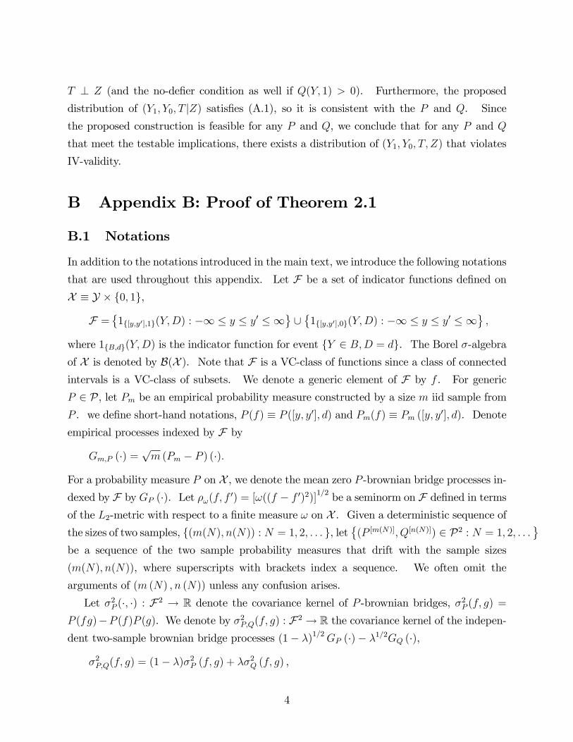
B Appendix B: Proof of Theorem 2.1

B.1 Notations

In addition to the notations introduced in the main text, we introduce the following notations

that are used throughout this appendix. Let F be a set of indicator functions de�ned on

X � Y � f0; 1g,

F =�1f[y;y0];1g(Y;D) : �1 � y � y0 � 1

[�1f[y;y0];0g(Y;D) : �1 � y � y0 � 1

;

where 1fB;dg(Y;D) is the indicator function for event fY 2 B;D = dg. The Borel �-algebraof X is denoted by B(X ). Note that F is a VC-class of functions since a class of connected

intervals is a VC-class of subsets. We denote a generic element of F by f . For generic

P 2 P, let Pm be an empirical probability measure constructed by a size m iid sample from

P . we de�ne short-hand notations, P (f) � P ([y; y0]; d) and Pm(f) � Pm ([y; y0]; d). Denoteempirical processes indexed by F by

Gm;P (�) =pm (Pm � P ) (�):

For a probability measure P on X , we denote the mean zero P -brownian bridge processes in-dexed by F by GP (�). Let �!(f; f 0) = [!((f � f 0)2)]

1=2 be a seminorm on F de�ned in termsof the L2-metric with respect to a �nite measure ! on X . Given a deterministic sequence ofthe sizes of two samples, f(m(N); n(N)) : N = 1; 2; : : : g, let

�(P [m(N)]; Q[n(N)]) 2 P2 : N = 1; 2; : : :

be a sequence of the two sample probability measures that drift with the sample sizes

(m(N); n(N)), where superscripts with brackets index a sequence. We often omit the

arguments of (m (N) ; n (N)) unless any confusion arises.

Let �2P (�; �) : F2 ! R denote the covariance kernel of P -brownian bridges, �2P (f; g) =P (fg)�P (f)P (g). We denote by �2P;Q(f; g) : F2 ! R the covariance kernel of the indepen-dent two-sample brownian bridge processes (1� �)1=2GP (�)� �1=2GQ (�),

�2P;Q(f; g) = (1� �)�2P (f; g) + ��2Q (f; g) ,

4

and �2Pm;Qn(�; �) be its sample analogue,

�2Pm;Qn(f; g) = (1� �̂) [Pm(fg)� Pm(f)Pm(g)] + �̂ [Qn(fg)�Qn(f)Qn(g)] .

Note that, with the current notation, �2Pm;Qm ([y; y0] ; d) de�ned in the main text is equivalent

to �2Pm;Qn(f; f), for f = 1f[y;y0];dg. For a sequence of random variables fWN : N = 1; 2; : : : gwhose probability law is governed by a sequence of two sample probability measures (P [m(N)]; Q[n(N)]);

WN �!P [m];Q[n]

c denotes convergence in probability in the sense of, for every � > 0,

limN!1

PrP [m];Q[n]

(jWN � cj > �) = 0:

In particular, if WN �!P [m];Q[n]

0, we notate as WN = oP [m];Q[n](1).

B.2 Auxiliary Lemmas

We �rst present a set of lemmas to be used in the proofs of Theorems 2.1 and 2.2.

Lemma B.1 Let�P [m] 2 P : m = 1; 2 : : :

be a sequence of probability measures on X .

Then,

supf2F

���P [m]m � P [m]�(f)�� �!P [m]

0:

Proof. F is the class of indicator functions corresponding to the interval VC-class of subsets,so an application of the Glivenko-Cantelli theorem uniform in P (Theorem 2.8.1 of van der

Vaart and Wellner (1996)) yields the claim.

Lemma B.2 Suppose Condition-RG. Let�P [m] 2 P : m = 1; 2 : : :

be a sequence of data

generating processes on X that weakly converges to P0 2 P as m!1. Then,

supB2B(X )

���P [m] � P0� (B)��! 0 as m!1.

Proof. We �rst consider the case of � being the Lebesgue measure. Suppose the conclusion

is false, that is, there exists � > 0 and a sequence fBm 2 B(X ) : m = 1; 2; : : : g such thatlim supm!1

���P [m] � P0� (Bm)�� > �. By uniform tightness of Condition-RG (b), there existsa compact set K 2 B(X ) such that

lim supm!1

���P [m] � P0� (Bm \K)�� > �=25

holds. Let fbmg be a subsequence of fmg such that���P [bm] � P0� (Bbm \K)�� > �=2 holds for

all bm � b�m. We metricize B (X ) by the L1-metric, dB(X )(B;B0) = (�� �d)(B4B0); where� is the measure de�ned in Condition-RG (a) and �d is the mass measure on d 2 f0; 1g.Since fBbm \K : m = 1; 2 : : : ; g is a sequence in a compact subset of B (X ), there exists asubsequence cbm of bm, such that

�Bcbm \K

converges to B� 2 B (X ) in terms of metric

dB(X )(�; �); and���P [cbm ] � P0� �Bcbm \K��� > �=2 (B.1)

holds by the construction of fbmg for all cbm � cb�m . Under the bounded density assumptionof Condition-RG (a), it holds that���P [cbm ] � P0� �Bcbm \K�� �P [cbm ] � P0� (B�)��

� 2MdB(X )(Bcbm \K;B�)! 0, as m!1.

Hence, (B.1) implies

lim supm!1

���P [cbm ] � P0� (B�)�� > �=2. (B.2)

Since � is the Lebesgue measure and, by Condition-RG (a), P0 as a weak limit of�P [m] : m = 1; 2; : : :

is absolutely continuous in �� �d, we have P0 (�B�) = 0 where �B� is the boundary of B�.Accordingly, by applying the Portmanteau theorem (see, e.g., Theorem 1.3.4 of van der

Vaart and Wellner (1996)), we obtain limm!1���P [m] � P0� (B�)�� = 0. This contradicts

(B.2). Hence, limm!1 supB2B(X )���P [m] � P0� (B)�� = 0 holds.

When � is a discrete mass measure with �nite support points, then the weak convergence

of P [m] to P0 is equivalent to the point wise convergence of the probability mass functions,

and the supB2B(X )���P [m] � P0� (B)�� is equivalent to the supremum over power sets of the

�nite support points. Hence, the claim follows.

For the case of � being a mixture of the Lebesgue and a discrete mass measure with �nite

support points, the claim holds as an immediate corollary of each of the two cases already

shown.

Lemma B.3 Suppose Condition-RG. Let�P [m] 2 P : m = 1; 2 : : :

be a sequence of data

generating processes on X that weakly converges to P0 2 P as m!1.

supf2F

���P [m]m � P0�(f)�� �!P [m]

0:

6

Proof. This lemma is a corollary of Lemma B.1 and B.2.

Lemma B.4 Suppose Condition-RG. Let�(P [m(N)]; Q[n(N)]) 2 P2 : N = 1; 2; : : :

be a se-

quence of two-sample probability measures with sample size (m;n) = (m(N); n(N)) !(1;1) as N !1. We have

supf;g2F

����2P[m]m ;Q

[m]n(f; g)� �2P [m];Q[m](f; g)

��� �!P [m];Q[n]

0:

Proof. Consider����2P[m]m ;Q

[m]n(f; g)� �2P [m];Q[m](f; g)

��� (B.3)

� (1� �)��P [m]m (fg)� P [m]m (f)P [m]m (g)� P [m](fg) + P [m](f)P [m](g)

��+���Q[n]n (fg)�Q[n]n (f)Q[n]n (g)�Q[n](fg) +Q[n](f)Q[n](g)��+ o(1);

where o(1) is the approximation error of order����̂� ����. Regarding the �rst term in the

right-hand side of this inequality, the following inequalities hold,

(1� �)��P [m]m (fg)� P [m]m (f)P [m]m (g)� P [m](fg) + P [m](f)P [m](g)

���

���P [m]m � P [m]�(fg)

��+ ��P [m]m (f)P [m]m (g)� P [m](f)P [m](g)��

����P [m]m � P [m]

�(fg)

��+ ���P [m]m � P [m]�(f)P [m]m (g)

��+ ���P [m]m � P [m]�(g)P [m](f)

���

���P [m]m � P [m]�(fg)

��+ ���P [m]m � P [m]�(f)��+ ���P [m]m � P [m]

�(g)�� : (B.4)

The second and the third term of (B.4) is oP [m] (1) uniformly in F by Lemma B.1. Further-more, since class of indicator functions ffg : f; g 2 Fg is also a VC-class,

supf;g2F

���P [m]m � P [m]�(fg)

�� �!P [m]

0

holds also by Lemma B.1. This proves the �rst term in the right-hand side of (B.3) converges

to zero uniformly in f; g 2 F . So is the case for the second term of (B.3) by the same

argument. Hence, the conclusion follows.

Lemma B.5 Suppose Condition-RG. Let�P [m] 2 P : m = 1; 2; : : :

be a sequence of proba-

bility measures, which converges weakly to P0 2 P. Then, the empirical processes Gm;P [m] (�)on index set F converge weakly to P0-brownian bridges GP0 (�).

7

Proof. To prove this lemma, we apply a combination of Theorem 2.8.3 and Lemma 2.8.8 of

van der Vaart and Wellner (1996) restricted to a class of indicator functions. It claims that,

given F be a class of measurable indicator functions and a sequence of probability measure�P [m] : m = 1; 2; : : :

in P, if (i)

R 10supR

plogN (�;F ; L2 (R))d� <1; where R ranges over

all �nitely discrete probability measures and N (�;F ; L2 (R)) is the covering number of Fwith radius � in terms of L2 (R)-metric [R(jf � f 0j2)]1=2,1 and (ii) there exists P � 2 P suchthat limm!1 supf;g2F fj�P [m](f; g)� �P �(f; g)jg = 0, then Gm;P [m] (�) weakly converges toP �-brownian bridge process GP � (�). Condition (i) is known to hold if F is a VC-class (see

Theorem 2.6.4 of van der Vaart and Wellner (1996)).

Therefore, what remains to show is Condition (ii). By the construction of seminorm

�P (f; g), we have

supf;g2F

���2P [m](f; g)� �2P0(f; g)�� � supB2B(X )

���P [m] � P0� (B)�� .Hence, to validate Condition (ii) with P � = P0, it su¢ ces to have limm!1 supB2B(X )

���P [m] � P0� (B)�� =0; which follows from Lemma B.2.

Lemma B.6 Suppose Condition-RG. Let�(P [m(N)]; Q[n(N)]) 2 P2 : N = 1; 2; : : :

be a se-

quence of probability measures of the independent two samples, which converges weakly to

(P0; Q0), as N !1. Then, stochastic processes indexed by VC-class of indicator functionsF ,

vN(�) =

�1� �̂

�1=2Gm;P [m] (�)� �̂

1=2Gn;Q[n](�)

� _ �P[m]m ;Q

[n]n(�; �) , � > 0, (B.5)

converges weakly to mean zero Gaussian processes v0(�) =(1��)1=2GP0 (�)��

1=2GQ0 (�)�_�P0;Q0 (�;�)

; where GP0 (�)and GQ0(�) are independent brownian bridge processes.

Proof. VC-class F is totally bounded with seminorm �P for any �nite measure P . Hence,

following Section 2.8.3 of van der Vaart and Wellner (1996), what we want to show for the

weak convergence of vN(�) are that (i) �nite dimensional marginal, (vN(f1); : : : ; vN(fK)), con-verges to that of v0(�), (ii) vN(�) is asymptotically uniformly equicontinuous along a sequence

1The covering number N (�;F ; L2 (R)) is de�ned as the minimal number of balls of radious � needed tocover F .

8

of seminorms such as L2(P [m] + Q[n]) norm, �P [m]+Q[n](f; g) =��P [m] +Q[n]

� �(f � g)2

��1=2,

i.e., for arbitrary � > 0,

lim�&0

lim supN!1

P �P [m];Q[n]

sup

�P [m]+Q[n]

(f;g)<�

jvN(f)� vN(g)j > �!= 0; (B.6)

where P �P [m];Q[n]

is the outer probability, and (iii) supf;g2F���P [m]+Q[n](f; g)� �P0+Q0(f; g)��! 0

as N ! 1. Note that (i) is implied by Lemma B.4 and Lemma B.5, and (iii) follows as acorollary of Lemma B.2, since

supf;g2F

����2P [m]+Q[n](f; g)� �2P0+Q0(f; g)��� � supB2B(X )

���P [m] � P0� (B)��+ supB2B(X )

���Q[n] �Q0� (B)��! 0 as N !1:

To verify (ii), consider, for f; g 2 F with �P [m]+Q[n](f; g) < �,

jvN(f)� vN(g)j (B.7)

������ 1

� _ �P[m]m ;Q

[n]n(f; f)

� 1

� _ �P[m]m ;Q

[n]n(g; g)

����� ���(1� �)1=2Gm;P [m] (g)� �1=2Gn;Q[n](g)���+(1� �)1=2

��Gm;P [m] (f)�Gm;P [m] (g)��+ �1=2 ��Gn;Q[n](f)�Gn;Q[n](g)��� _ �

P[m]m ;Q

[n]n(g; g)

+o�����̂� ����� :

Note that ����� 1

� _ �P[m]m ;Q

[n]n(f; f)

� 1

� _ �P[m]m ;Q

[n]n(g; g)

�����=

���� 1

� _ �P [m];Q[n](f; f)� 1

� _ �P [m];Q[n](g; g)

����+ oP [m];Q[n](1)� 1

�2��� _ �P [m];Q[n](f; f)� � _ �P [m];Q[n](g; g)��+ oP [m];Q[n](1)

� 1

�2���P [m];Q[n](f; f)� �P [m];Q[n](g; g)��+ oP [m];Q[n](1); (B.8)

where the �rst line follows from Lemma B.4. By noting the following inequalities,���P [m];Q[m](f; f)� �P [m];Q[m](g; g)��2�

����P[m]m ;Q

[m]n(f; f)� �P [m];Q[m](g; g)

��� ����P[m]m ;Q

[m]n(f; f) + �P [m];Q[m](g; g)

���=

����2P [m];Q[m](f; f)� �2P [m];Q[m](g; g)���9

and ����2P [m];Q[m](f; f)� �2P [m];Q[m](g; g)��� ���(1� �) �P [m](f)� P [m](g)� (1� P [m](f)� P [m](g))��+��� �Q[n](f)�Q[n](g)� (1�Q[n](f)�Q[n](g))��

���(1� �) �P [m](f)� P [m](g)���+ ��� �Q[n](f)�Q[n](g)���

� (1� �)�2P [m](f; g) + ��2Q[n](f; g)

� �2P [m]+Q[n](f; g);

we have���P [m];Q[m](f; f)� �P [m];Q[m](g; g)�� � �P [m]+Q[n](f; g). (B.9)

Combining (B.8) and (B.9) then leads to����� 1

� _ �P[m]m ;Q

[n]n(f; f)

� 1

� _ �P[m]m ;Q

[n]n(g; g)

����� � �P [m]+Q[n](f; g)

�2+ oP [m];Q[m](1) (B.10)

Hence, (B.7) and (B.10) yield

sup�P [m]+Q[n]

(f;g)<�

jvN(f)� vN(g)j ��

�2

���(1� �)1=2Gm;P [m] (g)� �1=2Gn;Q[n](g)��� (B.11)

+(1� �)1=2

�sup

�P [m]+Q[n]

(f;g)<�

��Gm;P [m] (f)�Gm;P [m] (g)��+�1=2

�sup

�P [m]+Q[n]

(f;g)<�

��Gn;Q[n](f)�Gn;Q[n](g)��+ oP [m];Q[m](1).Since �P [m](f; g) � �P [m]+Q[n](f; g) for every f; g 2 F , we have

sup�P [m]+Q[n]

(f;g)<�

��Gm;P [m] (f)�Gm;P [m] (g)�� � sup�P [m]

(f;g)<�

��Gm;P [m] (f)�Gm;P [m] (g)��= o�P [m] (�) ;

where o�P [m]

(�) denotes the convergence to zero in outer probability along�P [m]

as � & 0,

and the equality follows since the uniform convergence ofGm;P [m] (f) as established by Lemma

B.5 implies

lim�&0

lim supm!1

P �P [m]

sup

�P [m]

(f;g)<�

��Gm;P [m] (f)�Gm;P [m] (g)�� > �!= 0.

Similarly, we obtain sup�P [m]+Q[n]

(f;g)<�

��Gn;Q[n](f)�Gn;Q[n](g)�� = o�Q[n] (�).10

Since���(1� �)1=2Gm;P [m] (g)� �1=2Gn;Q[n](g)��� converges weakly to the tight Gaussian processes,

(B.11) is written as

sup�P [m]+Q[n]

(f;g)<�

jvN(f)� vN(g)j = �OP [m];Q[n] (1) + o�P [m];Q[m](�) + oP [m];Q[m](1)

= o�P [m];Q[m](�)

where OP [m];Q[n] (1) stands for that limN!1 PrP [m];Q[n]

(jWN j > aN) = 0 for every diverging

sequence aN !1. This establishes the asymptotic uniform equicontinuity (B.6).

The next lemma states that the null hypothesis of our test de�ned by inequalities (1.1)

for every Borel set B can be reduced without loss of information to the hypothesis that

inequalities (1.1) hold for all connected intervals. This lemma is a direct corollary of Lemma

C1 in Andrews and Shi (2013).

Lemma B.7 P (B; 1) � Q(B; 1) � 0 and Q(B; 0) � P (B; 0) � 0 hold for every Borel set

B if and only if P (V; 1) � Q(V; 1) � 0 and Q(V; 0) � P (V; 0) � 0 hold for all V 2 V �f[y; y0] : �1 � y � y0 � 1g :

Proof. The only-if statement is obvious. To prove the if statement, we apply Lemma C1

of Andrews and Shi (2013). By viewing V as R and P (�; 1)�Q(�; 1) as � (�) in the notationof Lemma C1 of Andrews and Shi (2013), it follows that P (B; 1) � Q(B; 1) � 0 for all B

in the Borel �-algebra generated by V. Since the Borel �-algebra generated by V coincideswith B(Y), P (V; 1) � Q(V; 1) � 0 for every V 2 V implies P (B; 1) � Q(B; 1) � 0 for everyB 2 B(Y). The same results hold for the other inequalities Q(�; 0)� P (�; 0) � 0.

The next lemma shows that the version of testable implications with conditioning covari-

ates as given in (3.3) can be reduced without any loss of information to the unconditional

moment inequalities of (3.4).

Lemma B.8 Assume that Pr(Z = 1jX) is bounded away from zero and one, X-a.s. Then,

Pr(Y 2 B;D = 1jZ = 1; X)� Pr(Y 2 B;D = 1jZ = 0; X) � 0; (B.12)

Pr(Y 2 B;D = 0jZ = 0; X)� Pr(Y 2 B;D = 0jZ = 1; X) � 0:

11

hold for all B 2 B(Y), X-a.s. if and only if

E [�1 (D;Z;X) g(Y;X)] � 0;

E [�0 (D;Z;X) g(Y;X)] � 0; for all g(�; �) 2 G,

where �1, �0, and G are as de�ned in Section 3.2 of the main text.

Proof. By applying Theorem 3.1 of Abadie (2003) with conditioning of X, the �rst inequal-

ities of (B.12) can be equivalently written as

E [1 fY 2 Bg�1(D;Z;X)jX] � 0, X-a.s. (B.13)

Hence, the only-if statement immediately follows.

To show the if statement, we again invoke Lemma C1 in Andrews and Shi (2013). Let

us read R and � (�) of their notation as

V �([y; y0]� [x1; x01]� � � � �

�xdx ; x

0dx

�: �1 � y � y0 � 1;

�1 � xl � x0l � 1; l = 1; : : : ; dx

);

and � (�) = E [�1 (D;Z;X) 1 f(Y;X) 2 �g], respectively. By the assumption that Pr(Z =

1jX) is bounded away from zero and one, �1 is bounded X-a.s. Hence, the thus-de�ned � (�)satis�es the boundedness condition to apply Lemma C1 in Andrews and Shi (2013). More-

over, V meets the condition for a semiring. Hence, � (V ) = E [�1 (D;Z;X) 1 f(Y;X) 2 V g] �0 for all V 2 V implies � (C) = E [�1 (D;Z;X) 1 f(Y;X) 2 Cg] � 0 for all C in the Borel �-algebra generated by V. Since the Borel �-algebra generated by V coincides with B(Y�X),and any product set B � Vx, B 2 B(Y) and Vx 2 B(X), belongs to B(Y�X), it impliesE [1 fY 2 Bg�1(D;Z;X)1 fX 2 Vxg] � 0 for all B 2 B(Y) and Vx 2 B(X). Hence, (B.13)

follows. A similar line of reasoning yields the equivalence of the second inequalities of (B.12)

to E [�0 (D;Z;X) g(Y;X)] � 0 for all g(�; �) 2 G.

B.3 Proof of Theorem 2.1

LetF1 =�1f[y;y0];1g(Y;D) : �1 � y � y0 � 1

andF0 =

�1f[y;y0];0g(Y;D) : �1 � y � y0 � 1

:

We want to show

lim supN!1

sup(P;Q)2H0

Pr (TN > cN;1��) � �; (B.14)

12

where

TN = max

8>><>>:supf2F1

��̂1=2Qn(f)�(1��̂)1=2Pm(f)�_�Pm;Qn (f;f)

�supf2F0

��(1��̂)1=2Pm(f)��̂

1=2Qn(f)

��_�Pm;Qn (f;f)

�9>>=>>; .

Consider a sequence�P [m(N)]; Q[n(N)]

�2 H0 at which PrP [m(N)];Q[n(N)] (TN > cN;1��) di¤ers

from its supremum overH0 by �N > 0 or less with �N ! 0 asN !1. Since�P [m(N)]; Q[n(N)]

�2

P2 are sequences in the uniformly tight class of probability measures (Condition-RG (b)),

there exists aN subsequence ofN such that�P [m(aN )]; Q[n(aN )]

�converges weakly to (P0; Q0) 2

P2 as N ! 1. Note that (P0; Q0) lies in H0 since�P [m(N)]; Q[n(N)]

�2 H0 for all N and

by Lemma B.2. With abuse of notations, we read aN as N and (m(aN); n(aN)) as (m;n)

with m+n = N . Along such sequence, we aim to show lim supN!1

PrP [m];Q[n] (TN > cN;1��) � �holds.

Using the notation of the weighted empirical processes introduced in Lemma B.6, we

can write the test statistic as

TN = max

(supf2F1 f�vN(f)� hN(f)gsupf2F0 fvN(f) + hN(f)g

);

where

hN (f) =

rmn

N

P [m](f)�Q[n] (f)� _ �

P[m]m ;Q

[n]n(f; f)

, d = 1; 0.

By the almost sure representation theorem (see, e.g., Theorem 9.4 of Pollard (1990)), weak

convergence of�vN(�); P [m]m (�); Q[n]n (�); �2

P[m]m ;Q

[n]n

(�; �)�to�v0(�); P0(�); Q0(�); �2P0;Q0(�; �)

�; as es-

tablished in Lemma B.3, B.4, and B.6, implies existence of a probability space (;B();P)and random objects ~v0 (�), ~vN (�), ~P [m]m (�), ~Q[n]n (�), and ~�2

P[m]m ;Q

[n]m(�; �) de�ned on it, such that

(i) ~v0 (�) has the same probability law as v0 (�) (ii)�~vN (�) ; ~P [m]m (�); ~Q[n]n (�); ~�2

P[m]m ;Q

[n]n(�; �)

�has

the same probability law as�vN (�) ; P [m]m (�); Q[n]n (�); �2

P[m]m ;Q

[n]n

(�; �)�for all N , and (iii)

supf2F

j~vN (f)� ~v0 (f)j ! 0; (B.15)

supf2F

��� ~P [m]m (f)� P0(f)��� ! 0, (B.16)

supf2F

��� ~Q[n]n (f)�Q0(f)��� ! 0, and (B.17)

supf;g2F

���~�2P[m]m ;Q

[n]m(f; g)� �2P0;Q0 (f; g)

��� ! 0, as N !1, P-a.s. (B.18)

13

Let ~TN be the analogue of TN de�ned on probability space (;B();P),

~TN = max

8<: supf2F1

n�~vN(f)� ~hN(f)

osupf2F0

n~vN(f) + ~hN(f)

o 9=; ;where ~hN(f) =

pmnN

P [m](f)�Q[n](f)�_~�2

P[m]m ;Q

[n]n

(f;f). Let ~cN;1�� be the bootstrap critical values, which we

view as a random object de�ned on the same probability space as�~vN ; ~P

[m]m ; ~Q

[n]n ; ~�

2

P[m]m ;Q

[n]n

�are de�ned. Note that the probability law of ~cN;1�� under P is identical to the probabilitylaw of bootstrap critical value cN;1�� under

�P [m]; Q[n]

�for everyN , because the distributions

of ~cN;1�� and cN;1�� are determined by the distributions of�~P[m]m ; ~Q

[n]n

�and

�P[m]m ; Q

[n]n

�,

respectively, and�~P[m]m ; ~Q

[n]n

���P[m]m ; Q

[n]n

�for every N , as claimed by the almost sure

representation theorem.

By the Lemma C.1 shown below, ~cN;1�� ! c1�� as N ! 1, P-a.s., where c1�� is the(1� �)-th quantile of statistic

TH � max(supf2F1 f�GH0(f)= (� _ �H0 (f; f))gsupf2F0 fGH0(f)= (� _ �H0 (f; f))g

), (B.19)

where H0 = �P0 + (1� �)Q0.Since PrP [m];Q[n] (TN > cN;1��) = P

�~TN > ~cN;1��

�for all N and ~cN;1�� ! c1�� as N !

1, P-a.s, if there exists a random variable ~T � de�ned on (;B();P), such that

(A) : lim supN!1

~TN � ~T �, P-a.s., and

(B) : The cdf of ~T � is continuous at c1�� and P�~T � > c1��

�� �,

then, the claim of the proposition follows from

lim supN!1

PrP [m];Q[n]

(TN > cN;1��) = lim supN!1

P�~TN > ~cN;1��

�� P

�~T � > c1��

�� �,

where the second line follows from Fatou�s lemma. Hence, in what follows, we aim to �nd

a random variable ~T � that satis�es (A) and (B).

14

Let �N be a deterministic sequence that satis�es �N !1 and �N=pN ! 0. Fix ! 2

and de�ne a sequence of subclass of F1,

F1;�N =nf 2 F1 : ~hN(f) � �N

o=

(f 2 F1 :

q�̂(1� �̂) P

[m](f)�Q[n](f)� _ ~�2

P[m]m ;Q

[n]n(f; f)

� �NpN

).

The �rst term in the maximum operator of ~TN satis�es

supf2F1

n�~vN(f)� ~h1;N(f)

o= max

8<: supf2F1;�N

n�~vN(f)� ~hN(f)

osupf2F1nF1;�N

n�~vN(f)� ~hN(f)

o 9=;� max

8<: supf2F1;�N f�~vN(f)gsupf2F1nF1;�N

n�~vN(f)� ~hN(f)

o 9=;� max

8>><>>:sup

f2[N0�N

F1;�N0f�~vN(f)g

supf2F1nF1;�N f�~vN(f)g � �N

9>>=>>; , (B.20)

for every N;where the second line follows since ~h1;N(f) � 0 for all f 2 F1 under the assump-tion that

�P [m]; Q[n]

�2 H0, the third line follows because ~hN(f) > �N for all f 2 F1 nF1;�N .

Since ~vN(�) is P-a.s. bounded and �N !1, it holds

supf2F1nF1;�N

f�~vN(f)g � �N ! �1; as N !1, P-a.s. (B.21)

On the other hand, since ~vN(�) P-a.s converges to ~v0 (�) uniformly in F , we have

sup

f2[N0�N

F1;�N0

f�~vN(f)g ! supf2F1;1

f�~v0 (f)g , as N !1; P-a.s., (B.22)

where F1;1 = limN!1[N 0�N

F1;�N0 . Let F�1 = ff 2 F1 : P0(f) = Q0(f)g. By the construc-

tion of F1;�N , every f 2 F1;1 satis�es

lim infN!1

(q�̂(1� �̂) P

[m](f)�Q[n](f)� _ ~�2

P[m]m ;Q

[n]n(f; f)

)= 0. (B.23)

Since P [m](f)�Q[n](f) converges to P0(f)�Q0(f) by Lemma B.2, any f satisfying (B.23)belongs to F�

1 . Hence, we have

supf2F1;1

f�~v0 (f)g � supf2F�1

f�~v0 (f)g P-a.s. (B.24)

15

By combining (B.20), (B.21), (B.22), and (B.24), we obtain

lim supN!1

supf2F1

n�~vN(f)� ~hN(f)

o� sup

f2F�1f�~v0 (f)g , P-a.s.

In a similar manner, it can be shown that

lim supN!1

supf2F0

n~vN(f) + ~hN(f)

o� sup

f2F�0f~v0 (f)g ; P-a.s.,

where F�0 = ff 2 F0 : P0(f) = Q0(f)g. Hence, ~T � de�ned by

~T � = max

(supf2F�1 f�~v0(f)gsupf2F�0 f~v0(f)g

)satis�es condition (A).

Next, we show that the thus-de�ned ~T � satis�es (B). First, we show that ~T � is stochas-

tically dominated by TH . Note that statistic TH de�ned in (B.19) can be written as

TH = max

(T �H ; sup

f2F1nF�1

�� GH0(f)

� _ �H0 (f; f)

�; supf2F0nF�0

�GH0(f)

� _ �H0 (f; f)

�),

where T �H = max

(supf2F�1 f�GH0(f)= (� _ �H0 (f; f))g ;supf2F�0 fGH0(f)= (� _ �H0 (f; f))g

).

If the distribution of T �H is identical to ~T�, then the distribution of TH stochastically domi-

nates ~T � so that we can ascertain the second part of (B). Hence, in what follows we show

that T �H and ~T � follow the same probability law. De�ne stochastic processes de�ned on

subdomain of F , F� = F�1 [ F�

0 ,

u(f) = �v0(f)1 ff 2 F�1g+ v0(f)1 ff 2 F�

0g ;

uH(f) = � GH0(f)

� _ �H0 (f; f)1ff 2 F�

1g+GH0(f)

� _ �H0 (f; f)1ff 2 F�

0g.

Note �rst that, for f 2 F�, P0(f) = Q0(f) = H0(f) implies that

�2P0;Q0(f; f) = P0(f)(1� P0(f)) = �2H0(f; f) .

Hence, V ar(u(f)) = V ar(uH(f)) holds for every f 2 F�. To also show equivalence of the

covariance kernels of u(�) and uH(�); consider, for f; g 2 F�;

Cov(u(f); u(g)) =(1� �) [P0(fg)� P0(f)P0(g)] + � [Q0(fg)�Q0(f)Q0(g)]

(� _ �P0;Q0 (f; f)) (� _ �P0;Q0 (g; g))

=[(1� �)P0 + �Q0] (fg)�H0(f)H0(g)(� _ �H0 (f; f)) (� _ �H0 (g; g))

:

16

If f 2 F�1 and g 2 F�

0 , P0 (fg) = Q0(fg) = H0(fg) = 0. If f; g 2 F�1 , then (P0; Q0) 2 H0

implies 0 � (P0 �Q0) (fg) � (P0 �Q0) (f) = 0, so P0 (fg) = Q0(fg) = H0(fg). Similarly,if f; g 2 F�

0 , (P0; Q0) 2 H0 implies 0 � (P0 �Q0) (fg) � (P0 �Q0) (f) = 0, so P0 (fg) =Q0(fg) = H0(fg) holds as well. Thus, we obtain

Cov(u(f); u(g)) =H0(fg)�H0(f)H0(g)

(� _ �H0 (f; f)) (� _ �H0 (g; g))= Cov(uH(f); uH(g))

for every f; g 2 F�. Equivalence of the covariance kernels imply equivalence of the prob-

ability laws of the mean zero Gaussian processes, so we conclude T �H � ~T �. Hence,

P�~T � > c1��

�� Pr(TH > c1��) = �.

To check the �rst requirement of (B), we show continuity of the cdf of ~T � at c1�� by

applying the absolute continuity theorem for the supremum of Gaussian processes (Tsirelson

(1975)), which says the supremum of Gaussian processes has a continuous cdf except at the

left limit of its support. By the de�nition of uH (�), TH can be equivalently written as

TH = supf2F fuH (f)g. Note �rst that the support of TH contains 0 since F contains an

indicator function for a singleton set in X at which uH0 (f) = 0 holds with probability one.

Following the symmetry argument of the mean zero Gaussian process, which we borrowed

from the proof of Proposition 2.2 in Abadie (2002), we have

Pr(TH � 0) = Pr ((@f 2 F ; uH (f) > 0)) = Pr ((@f 2 F ; uH (f) < 0)) :

By Condition-RG (a), uH (�) is not a degenerate process, so

Pr ((@f 2 F ; uH (f) < 0) \ (@f 2 F ; uH (f) < 0)) = 0:

Hence,

1 � Pr ((@f 2 F ; uH (f) < 0) [ (@f 2 F ; uH (f) < 0))

= 2Pr(TH � 0);

implying that the probability mass that TH can have at the left limit of its support is less

than or equal to 1=2. As a result, c1�� for � 2 (0; 1=2) lies in the region where the cdf of THis continuous. Since ~T � is also a supremum of mean zero Gaussian process and, as already

shown, it is stochastically dominated by TH , the cdf of ~T � is also continuous at c1��. This

completes the proof of Theorem 2.1 (i).

17

To prove claim (ii), assume that the �rst inequality of (1.1) is violated for some Borel

set B � Y. By lemma B.7, there exists some f � 2 F1 such that 0 � P (f �) < Q(f �) holds.Then, we have

TN = max

8>><>>:supf2F1

��̂1=2Qn(f)�(1��̂)1=2Pm(f)�_�Pm;Qn (f;f)

�supf2F0

�(1��̂)1=2Pm(f)��̂

1=2Qn(f)

�_�Pm;Qn (f;f)

�9>>=>>;

�

��̂1=2Gn;Q(f

�)� (1� �̂)1=2Gm;P (f �)�

� _ �Pm;Qn(f �; f�)+

rmn

N

Q(f �)� P (f �)� _ �Pm;Qn(f �; f�)

; (B.25)

where the second term of (B.25) diverges to positive in�nity, while the �rst term is sto-

chastically bounded asymptotically. Since the bootstrap critical values cN;1�� converges to

c1�� < 1 irrespective of the null holds true or not, the rejection probability converges to

one.

C Convergence of the Bootstrap Critical Values and a

Proof of Theorem 2.2

C.1 A Lemma on Convergence of the Bootstrap Critical Values

The proof of Theorem 2.1 given in the previous section assumes P-almost sure convergenceof the bootstrap critical value ~cN;1�� to c1��. This convergence claim is proven by the next

lemma. The probability space (;B();P) and the random objects with "tilde" used in

the following proof are the ones de�ned in the proof of Theorem 2.1 (i) by the almost sure

representation theorem.

Lemma C.1 Suppose Condition-RG. Let ~cN;1�� be the bootstrap critical value of Algorithm

2.1 constructed from ~H[N ]N = �̂ ~P

[m]m + (1 � �̂) ~Q[n]n ; which is viewed as a sequence of random

variables f~cN;1�� : N = 1; 2; : : : g de�ned on probability space (;B();P). It holds that

~cN;1�� converges to c1�� as N !1, P-a.s, where c1�� is the (1� �)-th quantile of statistic

TH = max

(supf2F1 f�GH0(f)= (� _ �H0 (f; f))gsupf2F0 fGH0(f)= (� _ �H0 (f; f))g

),

18

where H0 = �P0 + (1� �)Q0.

Proof. Let sequencen~H[N ]N : N = 1; 2; : : :

obe given, and let P �m and Q

�n be the bootstrap

empirical probability measures with size m and size n; respectively, drawn iid from ~H[N ]N .

De�ne bootstrap weighted empirical processes indexed by f 2 F as

v�N(�) =

rmn

N

P �m(�)�Q�n(�)� _ �P �m;Q�n(�; �)

=(1� �̂)1=2G�

m; ~H[N ]N

(�)� �̂1=2G�0n; ~H

[N ]N

(�)(f)

� _ �P �m;Q�n(�; �);

where G�m; ~H

[N ]N

(�) =pm�P �m � ~H

[N ]N

�(�) and G�0

n; ~H[N ]N

(�) =pn�Q�n � ~H

[N ]N

�(�) are two in-

dependent bootstrap empirical processes givenn~H[N ]N : N = 1; 2; : : :

o. Let (X1; : : : ; XN)

be the N support points of ~H [N ]N , and let �X be the point-mass measure at X. To apply

the uniform central limit theorem with exchangeable multipliers (Theorem 3.6.13 of van der

Vaart and Wellner (1996)), we introduce multinomial random vector (Mm;1; : : : ;Mm;N) that

is independent of (X1; : : : ; XN) and has parameters�m; 1

N; : : : ; 1

N

�. We express G�

m; ~H[N ]N

(�)as

G�m; ~H

[N ]N

(�) =1pm

NXi=1

�Mm;i �

m

N

��Xi (�)

=1pm

NXi=1

�Mm;i �

m

N

� ��Xi �H [N ]

�(�)

= �̂�1=2 1p

N

NXi=1

�m;i��Xi �H [N ]

�(�) ;

where �m;i = Mm;i � mN, i = 1; : : : ; N . Note that

��m;1; : : : ; �m;N

�are exchangeable ran-

dom variables by construction and E�1N

PNi=1 �

2i

�= m

N

�1� 1

N

�! �; as N ! 1. On

the other hand, since H [N ] converges weakly to H0, an application of Lemma B.5 yields1pN

PNi=1

��Xi �H [N ]

�(�) GH0 (�). Hence, the uniform central limit theorem with ex-

changeable multipliers (Theorem 3.6.13 of van der Vaart and Wellner (1996)) leads to

G�m; ~H

[N ]N

(�) GH0 (�) for P-almost every sequencen~H[N ]N : N = 1; 2; : : :

o. By the same

reasoning, we have G�0n; ~H

[N ]N

(�) G0H0 (�) for P-almost every sequencen~H[N ]N : N = 1; 2; : : :

o,

where G0H0 (�) is an H0-brownian bridge process independent of GH0 (�).

19

Hence, the numerator of v�N(�) converges weakly to (1��)1=2GH0 (�)��1=2G0H0 (�), P-a.s.sequences of

n~H[N ]N

o. Note that the covariance kernel of (1 � �)1=2GH0 (�) � �1=2G0H0 (�)

coincides with that of H0-brownian bridge, so we conclude that

(1� �̂)1=2G�m; ~H

[N ]N

(�)� �̂1=2G�0n; ~H

[N ]N

(�)(f) GH0 (�) , P-a.s. sequences ofn~H[N ]N

o. (C.1)

Regarding the bootstrap covariance kernel, we have convergence of supf2F���P �m;Q�n(f; f)� �H0 (f; f)��

to zero (in probability in terms of the probability law of bootstrap resampling given ~H[N ]N )

for P-a.s. sequences ofn~H[N ]N

o; since

supf2F

���2P �m;Q�n(f; f)� �2H0 (f; f)�� � supf2F

����2P �m;Q�n(f; f)� �2~H[N ]N

(f; f)���+sup

f2F

����2~H[N ]N

(f; f)� �2H0 (f; f)��� ;

(C.2)

where the �rst term in the right hand side converges to zero (in probability in terms of the

probability law of bootstrap resampling) by applying the Glivenko-Cantelli theorem for the

triangular arrays as given in Lemma B.1, and the convergence to zero P-a.s. for the secondterm follows from the almost sure representation theorem, (B.16) and (B.17).

By putting together (C.1) and (C.2), and repeating the proof of the asymptotic uniform

equicontinuity as given in (B.11) above, we obtain

v�N(�) (1� �)1=2GH0 (�)� �̂

1=2G0H0 (�)

� _ �H0(�; �)

� GH0 (�)� _ �H0(�; �)

; as N !1,

for P-almost every sequence ofn~H[N ]N

o. The bootstrap test statistics T �N is a continuous

functional of v�N(�), so the continuous mapping theorem leads to

T �N TH = max

(supf2F1 f�GH0(f)= (� _ �H0 (f; f))gsupf2F0 fGH0(f)= (� _ �H0 (f; f))g

)as N !1,

for P-almost every sequence ofn~H[N ]N

o. We already showed in the proof of Theorem 2.1

(i) that the cdf of TH is continuous at c1�� for � 2 (0; 1=2). Hence, the bootstrap critical

values ~cN;1�� converges to c1��, P-a.s.

20

C.2 Proof of Theorem 2.2

Proof. By Assumption-LA(c) and the Portmanteau theorem,�P [N ]; Q[N ] 2 P2 : N = 1; 2 : : :

�converges weakly to (P0; Q0) 2 H0. We can therefore apply all the lemmas established in

Appendix B and C.1, and, as done in the proof of Theorem 2.1 (i), we can de�ne via the

almost sure representation theorem a probability space (;B();P) and random objects

with "tilde", that copy the ones de�ned in a sequence of probability spaces in terms of�P [N ]; Q[N ] : N = 1; 2; : : :

�. By Lemma C.1, the bootstrap critical values ~cN;1�� converges

to c1�� the (1��)-th quantile of TH , P-a.s., which depends only on (�; �; �; P0; Q0). Suppose

that ([y; y0] ; d = 1) satis�es Assumption-LA (a) and (d). Let ~vN (�) =(1��̂)

1=2 ~Gm;P [N ]

(�)��̂1=2 ~Gn;Q[N ]

(�)�_~�

P[N ]m ;Q

[N ]n(�;�)

be the weighted empirical process de�ned on (;B();P), where ~Gm;P [N ] (�) =pm�~P[N ]m � P [N ]

�(�)

and ~Gm;Q[N ] (�) =pm�~Q[N ]n �Q[N ]

�(�). Note the probability law of the test statistic is that

of

~TN = max

8<: supf2F1

n�~vN(f)� ~hN(f)

osupf2F0

n~vN(f) + ~hN(f)

o 9=; ;induced by P, where

~hN (f) =

rmn

N

P [N ](f)�Q[N ] (f)� _ ~�

P[N ]m ;Q

[N ]n(f; f)

:

Since ~TN is bounded from below by

�~vN([y; y0] ; 1)� ~hN([y; y0] ; 1);

the rejection probability is also bounded from below by

P(�~vN([y; y0] ; 1)� ~hN([y; y0] ; 1) � ~cN;1��).

By Assumption-LA (c), and by applying Lemmas B.4 and B.6, ~vN([y; y0] ; 1)� ~hN([y; y0] ; 1)converges P-a.s. to

�~v0 ([y; y0] ; 1)�[�(1� �)]1=2��([y; y0] ; 1)� _ �P0;Q0 ([y; y0] ; 1)

;

21

which follows Gaussian with mean � [�(1��)]1=2��([y;y0];1)�_�P0;Q0 ([y;y0];1)

and variance minn�2P0;Q0

([y;y0];1)

�2; 1o.

Hence, we obtain

P(�~vN([y; y0] ; 1)� ~hN([y; y0] ; 1) � ~cN;1��)

! P(�~v0([y; y0] ; 1)�[�(1� �)]1=2��([y; y0] ; 1)� _ �P0;Q0 ([y; y0] ; 1)

� c1��)

= 1� � �

�2P0;Q0 ([y; y0] ; 1)

�2^ 1��1

c1�� �[�(1� �)]1=2 j��([y; y0] ; 1)j

� _ �P0;Q0 ([y; y0] ; 1)

!!:

In case ([y; y0] ; d = 0) satis�es Assumption-LA (i) and (iv), a similar argument yields the

same lower bound.

D Monte Carlo Studies

This section examines the �nite sample performance of the test by Monte Carlo. In assessing

�nite sample type I errors of the test, we consider a data generating process on a boundary

of H0, so that the theoretical type I error of the test equals to a nominal size asymptotically.

p(y;D = 1) = q(y;D = 1) = 0:5�N (1; 1);

p(y;D = 0) = q(y;D = 0) = 0:5�N (0; 1);

where N(�; �2) is the probability density of a normal random variable with mean � and �2.

In computing the �rst (second) supremum of the test statistic, the boundaries points of

intervals are chosen by every pair of Y -values observed in the subsample of fD = 1; Z = 0g(fD = 0; Z = 1g). In order to assess how the test performance depends on a choice of

trimming constant, we run simulations for each of the following four speci�cation of the

trimming constant,

�1 =p0:005 (1� 0:005) � 0:07;

�2 =p0:05(1� 0:05) � 0:22;

�3 =p0:1(1� 0:1) = 0:3;

�4 = 1:

Note that �k, k = 1; 2; 3, has the form ofp�k(1� �k), and �k can be interpreted as that,

if both Pm ([y; y0] ; d) and Qn ([y; y0] ; d) are less than �k, we weigh the di¤erence of the

empirical distribution by the inverse of � instead of the inverse of its standard deviation

22

Table 2: Monte Carlo Test Size

Monte Carlo iterations 1000, Bootstrap iterations 300.

Trimming constant �1 � 0:07 �2 � 0:21 �3 = 0:3 �4 = 1

Nominal size .10 .05 .01 .10 .05 .01 .10 .05 .01 .10 .05 .01

(m,n):(100,100) .13 .07 .01 .13 .07 .01 .14 .06 .01 .13 .06 .01

(100,500) .11 .06 .01 .10 .06 .01 .11 .05 .01 .10 .05 .01

(500,500) .13 .06 .02 .12 .07 .02 .11 .06 .02 .12 .05 .01

(100,1000) .12 .06 .02 .12 .06 .01 .13 .06 .02 .12 .06 .02

(1000,1000) .14 .07 .02 .13 .08 .02 .13 .06 .02 .12 .06 .01

Note: The statistic is equivalent to the non-weighted KS-statistics when �4 = 1:

estimate. Accordingly, as �k becomes larger, we put relatively less weight on the di¤erences

of the empirical probabilities for thinner probability events. The fourth choice of �, �4 = 1,

makes the test statistic identical to the non-weighted KS-statistic.

Table 2 shows the simulated test size. The rejection probabilities are slightly upward

biased relative to the nominal sizes, while they are overall showing good size performance

even in the cases with the sample sizes being as small as (m;n) = (100; 100) and being

unbalanced as much as (m;n) = (100; 1000). It is also worth noting that these test sizes are

not sensitive to a choice of trimming constant.

In order to see �nite sample power performance of our test, we simulate the rejection

probabilities of the bootstrap test against four di¤erent speci�cations of �xed alternatives.

These four data generating processes share

Pr(Z = 1) =1

2, Pr(D = 1jZ = 1) = 0:55, Pr(D = 1jZ = 0) = 0:45

p(y;D = 1) = 0:55�N (0; 1);

p(y;D = 0) = 0:45�N (0; 1); q(y;D = 0) = 0:55�N (0; 1);

while they di¤er in terms of speci�cations of the treated outcome distribution conditional

23

on Z = 0,

DGP 1: q(y;D = 1) = 0:45�N (�0:7; 1);

DGP 2: q(y;D = 1) = 0:45�N (0; 1:6752);

DGP 3: q(y;D = 1) = 0:45�N (0; 0:5152);

DGP 4: q(y;D = 1) = 0:45�5Xl=1

wlN (�l; 0:1252);

(w1; : : : ; w5) = (0:15; 0:2; 0:3; 0:2; 0:15) ;

(�1; : : : ; �5) = (�1;�0:5; 0; 0:5; 1) :

In all these speci�cations, violations of the testable implication occur only for the treatment

outcome densities. As plotted in Figure 6, the ways that the densities p(y; 1) and q(y; 1)

intersect di¤er across the DGPs. In DGP 1, p(y; 1) and q(y; 1) is di¤erentiated horizontally,

and they intersect only once. In DGP 2, the violations occurs at the tail parts of p(y; 1)

and q(y; 1), whereas, in DGP 3, the violation occurs around the modes of p(y; 1) and q(y; 1).

In DGP 4, q(y; 1) is speci�ed to be oscillating sharply around p(y; 1) and they intersect

many times. In all these speci�cations, p(y; 1) and q(y; 1) are designed to be equally distant

in terms of the one-sided total variation distance, i.e.,R1�1max f(q(y; 1)� p(y; 1)); 0g dy �

0:092 for all the DGPs.

Table 3 shows the simulated rejection probabilities, based on which several remarks follow.

First, we observe that the rejection probabilities vary depending on the DGPs and the choices

of trimming constant. When the violations occur for the tail parts of the densities (DGP2),

smaller � yields a signi�cantly higher power. In contrast, if violations occur on a fatter part

of the densities (DGPs 1, 3 and 4), middle-range ��s and � = 1 tend to exhibit a slightly

higher power than the smallest choice of �. This suggests that, if a likely violation of the

testable implications is expected at the tail parts of the distributions, it is important to

use a variance weighted statistic with a su¢ ciently small � such as � = 0:07: Given these

simulation �ndings that a power loss by choosing � = 0:07 instead of the medium size �

or � = 1 is not so severe in the other cases, we can argue that, in case there is no prior

knowledge available about a likely alternative, one default choice of � is as small as 0:07.

At the same time, it is also worth reporting the test results with several other choices of

� 2 (0; 0:5]. Second, the rows of unbalanced sample sizes indicate that the magnitude of

24

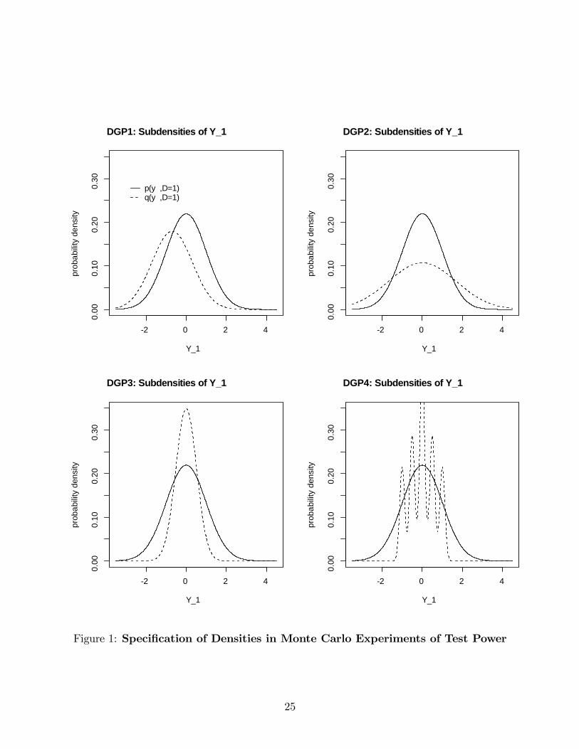
­2 0 2 4

0.00

0.10

0.20

0.30

DGP1: Subdensities of Y_1

Y_1

prob

abilit

y de

nsity

p(y ,D=1)q(y ,D=1)

­2 0 2 40.

000.

100.

200.

30

DGP2: Subdensities of Y_1

Y_1

prob

abilit

y de

nsity

­2 0 2 4

0.00

0.10

0.20

0.30

DGP3: Subdensities of Y_1

Y_1

prob

abilit

y de

nsity

­2 0 2 4

0.00

0.10

0.20

0.30

DGP4: Subdensities of Y_1

Y_1

prob

abilit

y de

nsity

Figure 1: Speci�cation of Densities in Monte Carlo Experiments of Test Power

25

the rejection probabilities tend to depend on a smaller sample size of (m;n), rather than

the total sample size N , so a lack of power should be acknowledged when one of the sample

size is small. Third, for the magnitudes of violations considered in these simulations, the

rejection probabilities are su¢ ciently close to one (for some smaller choices � only for DGP

2) if the sample sizes are as large as (m;n) = (1000; 1000).

References

[1] Abadie, A. (2002): "Bootstrap Tests for Distributional Treatment E¤ects in Instrumental

Variable Models," Journal of the American Statistical Association, 97, 284-292.

[2] Abadie, A. (2003): "Semiparametric Instrumental Variable Estimation of Treatment

Response Models," Journal of Econometrics, 113, 231 - 263.

[3] Andrews, D.W.K. and X. Shi (2013): "Inference Based on Conditional Moment Inequal-

ities," Econometrica, 81, 609-666.

[4] Dudley, R. M. (1999): Uniform Central Limit Theorem. Cambridge University Press.

[5] Pollard, D. (1990): Empirical Processes: Theory and Applications, NSF-CBMS Regional

Conference Series in Probability and Statistics, Vol. 2.

[6] Romano, J. P. (1988): "A Bootstrap Revival of Some Nonparametric Distance Tests."

Journal of American Statistical Association, 83, 698-708.

[7] Tsirelson, V.S. (1975): "The density of the maximum of a Gaussian Process," Theory of

Probability and Its Applications, 20, 817-856.

[8] van der Vaart, A. W., and J. A. Wellner (1996): Weak Convergence and Empirical

Processes: With Applications to Statistics, New York: Springer.

26

Table 3: Rejection Probabilities against Fixed Alternatives

Monte Carlo iterations 1000, Bootstrap iterations 300.

Trimming constant �1 � 0:07 �2 = 0:22 �3 = 0:3 �4 = 1

Nominal size .10 .05 .01 .10 .05 .01 .10 .05 .01 .10 .05 .01

DGP1 (m,n):(100,100) .31 .22 .10 .31 .21 .10 .30 .21 .10 .23 .15 .05

(100,500) .42 .31 .14 .56 .43 .22 .57 .44 .21 .38 .24 .07

(500,500) .93 .88 .77 .95 .91 .78 .96 .92 .79 .89 .80 .52

(100,1000) .38 .28 .12 .58 .46 .24 .59 .46 .23 .39 .26 .09

(1000,1000) .99 .98 .94 1.00 .99 .97 .99 .98 .94 .99 .98 .93

DGP2 (m,n):(100,100) .16 .09 .02 .15 .09 .02 .08 .04 .00 .01 .00 .00

(100,500) .35 .23 .07 .17 .10 .02 .07 .02 .00 .01 .00 .00

(500,500) .95 .91 .73 .86 .77 .53 .56 .40 .16 .10 .03 .01

(100,1000) .40 .26 .08 .20 .09 .02 .06 .03 .00 .01 .00 .00

(1000,1000) 1.00 1.00 1.00 1.00 .99 .97 .96 .90 .67 .52 .27 .05

DGP3 (m,n):(100,100) .30 .20 .09 .30 .20 .09 .33 .22 .09 .34 .22 .09

(100,500) .32 .21 .08 .51 .38 .19 .59 .46 .23 .55 .40 .15

(500,500) .77 .69 .54 .83 .76 .57 .87 .79 .62 .89 .82 .61

(100,1000) .30 .18 .06 .53 .40 .18 .61 .47 .25 .54 .41 .18

(1000,1000) .98 .96 .89 .99 .98 .93 1.00 .99 .96 1.00 .99 .95

DGP4 (m,n):(100,100) .12 .07 .02 .11 .07 .02 .09 .05 .02 .09 .05 .01

(100,500) .23 .13 .04 .20 .11 .03 .15 .09 .02 .12 .05 .01

(500,500) .46 .33 .17 .45 .33 .16 .33 .22 .10 .23 .13 .03

(100,1000) .26 .15 .05 .22 .13 .05 .15 .10 .03 .11 .06 .01

(1000,1000) .78 .67 .48 .80 .69 .50 .51 .38 .19 .45 .30 .11

27