A TEST OF MULTI-INDEX ASSET PRICING MODELS:

THE CASE OF ISTANBUL STOCK EXCHANGE

A THESIS SUBMITTED TO

THE GRADUATE SCHOOL OF SOCIAL SCIENCES

OF

MIDDLE EAST TECHNICAL UNIVERSITY

BY

SIRRI SELİM KALAÇ

IN PARTIAL FULFILLMENT OF THE REQUIREMENTS

FOR

THE DEGREE OF MASTER OF BUSINESS ADMINISTRATION

IN

THE DEPARTMENT OF BUSINESS ADMINISTRATION

SEPTEMBER 2012

 

 

Approval of the Graduate School of Social Sciences

Prof. Dr. Meliha Altunışık

Director

I certify that this thesis satisfies all the requirements as a thesis for the degree of

Master of Business Administration.

Assoc. Prof. Dr. Engin Küçükkaya

Head of Department

This is to certify that we have read this thesis and that in our opinion it is fully

adequate, in scope and quality, as a thesis for the degree of Master of Business

Administration.

Assist. Prof. Dr. Seza Danışoğlu

Supervisor

Examining Committee Members

Prof. Dr. Z. Nuray Güner (METU,BA)

Assist. Prof. Dr. Seza Danışoğlu (METU,BA)

Assoc. Prof. Dr. Zeynep Önder (Bilkent, MAN)

iii  

I hereby declare that all information in this document has been obtained and

presented in accordance with academic rules and ethical conduct. I also declare

that, as required by these rules and conduct, I have fully cited and referenced

all material and results that are not original to this work.

Name, Last Name: Sırrı Selim Kalaç

Signature : ____________________

iv  

ABSTRACT

A TEST OF MULTI-INDEX ASSET PRICING MODELS:

THE CASE OF ISTANBUL STOCK EXCHANGE

Kalaç, Sırrı Selim

MBA, Department of Business Administration

Supervisor : Assist. Prof. Dr. Seza Danışoğlu

September 2012, 73 pages

This study employs widely excepted asset pricing models to test their explanatory

power in the context of Istanbul Stock Exchange listed companies between 1990 and

2010. The risk factors, beta, size, book-to-market equity, and momentum are used to

form portfolios and their factor loadings are estimated. The results of this study are

mostly in line with the previous academic research, and some unique attributes of the

return generation mechanism of Istanbul Stock Exchange are reported.

Keywords: Capital Asset Pricing Model (CAPM), Multi-Index Asset Pricing Models,

Istanbul Stock Exchange, Risk Factors

v  

ÖZ

ÇOKLU-ENDEKS VARLIK FİYATLAMA MODELLERİNİN TESTİ:

İSTANBUL MENKUL KIYMETLER BORSASI UYGULAMASI

Kalaç, Sırrı Selim

Yüksek Lisans, İşletme Bölümü

Tez Yöneticisi : Yrd. Doç. Dr. Seza Danışoğlu

Eylül 2012, 73 sayfa

Bu çalışmada, yaygın olarak kabul görmüş varlık fiyatlama modellerinin istatistiksel

açıklama gücü İstanbul Menkul Kıymetler Borsası'nda 1990 - 2010 arasında işlem

gören hisseler üzerinde test edilmektedir. Risk faktörleri, beta, firma büyüklüğü,

defter-değeri-pazar-değeri oranı ve momentuma göre sıralanmış portföylerle, faktör

katsayıları hesaplanmıştır. Bu çalışmanın sonuçlarının büyük bölümü önceki

akademik çalışmaların sonuçlarıyla parallellik gösterse de, İstanbul Menkul

Kıymetler Borsası'na özgü kimi getiri mekanizmaları raporlanmıştır.

Anahtar Kelimeler: Yatırım Varlıklarını Fiyatlandırma Modeli, Çoklu-Endeks Varlık

Fiyatlandırma Modelleri, İstanbul Menkul Kıymetler Borsası, Risk Faktörleri

vi  

To my wife and our beautiful princess who supported me each step of the way.

vii  

ACKNOWLEDGMENTS

I would like to express my deepest gratitude to my supervisor, Assist. Prof. Dr. Seza

Danışoğlu, for her guidance, advice, criticism and insight throughout the

development of this thesis.

I would also like to thank Prof. Dr. Z. Nuray Güner and Assoc. Prof. Dr. Zeynep

Önder for their invaluable suggestions and comments.

I acknowledge my wife, Sebla Kömürcü Kalaç, for her continuous support and

invaluable encouragements all through this thesis. This study would have never been

realized without her help.

viii  

TABLE OF CONTENTS

PLAGIARISM.............................................................................................................iii

ABSTRACT................................................................................................................iv

ÖZ.................................................................................................................................v

DEDICATION.............................................................................................................vi

ACKNOWLEDGMENTS..........................................................................................vii

TABLE OF CONTENTS..........................................................................................viii

LIST OF TABLES........................................................................................................x

CHAPTER

1. INTRODUCTION...............................................................................................1

2. LITERATURE REVIEW....................................................................................3

3. DATA AND METHODOLOGY.......................................................................37

3.1. DATA......................................................................................................37

3.1.1. The Time Period, Frequency and Sources of Data...................37

3.1.2. Sample Filtering........................................................................38

3.2. METHODOLOGY..................................................................................39

3.2.1. Introduction...............................................................................39

3.2.2. Models and Determination of Independent Variables..............40

3.2.3. Determination of Dependent Variables....................................47

ix  

3.2.4. The Testing Procedure..............................................................49

3.2.5. Calculation of Performance Measures......................................50

3.2.6. Time Frame of Independent Variables

and Performance Comparison..................................................50

4. RESULTS AND ANALYSIS...........................................................................51

4.1. DETAILS ABOUT THE METHODOLOGY.........................................51

4.1.1. The Number of Stocks Used.....................................................51

4.1.2. Remarks About Book-to-Market Equity Based

Portfolio Formation...................................................................53

4.1.3. The Time Frame of Regressions...............................................53

4.2. RESULTS................................................................................................55

4.3.ANALYSIS..............................................................................................60

5. CONCLUSION.................................................................................................63

REFERENCES...........................................................................................................65

APPENDIX A: RESULTS SUMMARY TABLES FOR SUB-PERIOD

ESTIMATIONS...............................................................................69

APPENDIX B: TEZ FOTOKOPİ İZİN FORMU......................................................73

x  

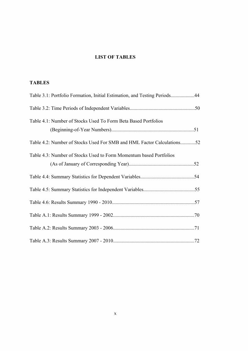
LIST OF TABLES

TABLES

Table 3.1: Portfolio Formation, Initial Estimation, and Testing Periods...................44

Table 3.2: Time Periods of Independent Variables....................................................50

Table 4.1: Number of Stocks Used To Form Beta Based Portfolios

(Beginning-of-Year Numbers)..................................................................51

Table 4.2: Number of Stocks Used For SMB and HML Factor Calculations............52

Table 4.3: Number of Stocks Used to Form Momentum based Portfolios

(As of January of Corresponding Year)....................................................52

Table 4.4: Summary Statistics for Dependent Variables...........................................54

Table 4.5: Summary Statistics for Independent Variables.........................................55

Table 4.6: Results Summary 1990 - 2010..................................................................57

Table A.1: Results Summary 1999 - 2002.................................................................70

Table A.2: Results Summary 2003 - 2006.................................................................71

Table A.3: Results Summary 2007 - 2010.................................................................72

1  

CHAPTER 1

INTRODUCTION

This study aims to estimate the single- and multi-index asset pricing models by using

time-series data from the Istanbul Stock Exchange. The testing of the asset pricing

models has been a favorable topic in the finance literature since the 1960s. Although

the search for the best pricing model still continues, today if the researchers or the

practitioners are asked to name the model that they use, they mostly quote the multi-

index models that have been in widespread use since the mid-1990s.

To any student of finance, the asset pricing debate starts with Markowitz’s Portfolio

Theory (1952), continues with Sharpe (1964), Lintner (1965), and Mossin (1966)

papers on the single-index Capital Asset Pricing Model, and finally settles into the

multi-index modeling proposed by the 1993 Fama and French and 1997 Carhart

studies. Even though all these models have been extensively tested in previous

studies for developed as well as emerging markets, no comprehensive testing and

comparison of the models have been conducted for the Turkish stock market.

Therefore, this study attempts to fill a gap in the literature by estimating all three

versions of the asset pricing model by using data from the Istanbul Stock Exchange.

The study aims to compare the performance of the models and produce estimates for

factor loadings that can be readily used by researchers in future studies.

In order to provide some further insight regarding the explanatory power of the

models employed, this study estimates factor loadings for three groups of portfolios,

each formed based on a different aspect of stock attributes. Furthermore, the possible

effect of the sample period is examined by sub-period analyses, in order to

investigate any deviation from the findings of the entire sample period. The reported

2  

findings imply a consistent return generation mechanism within Istanbul Stock

Exchange, regardless of the time interval chosen.

The empirical findings suggest that the multi-index models estimated for the Turkish

market perform as well as they do when they are estimated for the more developed

stock markets. The results imply that Turkish investors price the market-wide

systematic risk as well as the size, book-to-market, and momentum risks when they

make investment decisions. However, interestingly enough, the factor loadings for

the HML and WML risks have the opposite sign in the Turkish sample compared to

the sign estimates from the more developed markets. Namely, the book-to-market

equity risk has a negative factor loading (implying a preference for growth stock) and

the momentum factor also has a negative factor loading (indicating a preference for

contrarian strategies) in the Turkish stock market.

This study finds evidence in support of increased explanatory power with the

inclusion of new risk factors; however, this improvement is observed in the adjusted

R2 values, but not in the Jensen's Alpha values, a result that is in contrast to the

earlier studies. It is shown that the excess market return factor, even on its own, has a

very high explanatory power and it is not reduced with the inclusion of new factors

into the model. The mentioned findings are in line with the findings of earlier

research.

Last but not least, the findings of this study prove that, despite being a relatively

young and thin stock market, the prices in the Istanbul Stock Exchange seem to not

being generated arbitrarily, but through a mechanism. This return generation

mechanism has some common attributes with more established markets and others

characteristics that are unique to Istanbul Stock Exchange. The researcher hopes that

the findings of this study will raise new questions to be answered about the unique

features of the Istanbul Stock Exchange.

3  

CHAPTER 2

LITERATURE REVIEW

Markowitz (1952), along with his rigorous geometric demonstration, provides a

thorough understanding of portfolio formation under uncertain expected returns of

assets, in other words, when returns have a non-zero variance. The rule he prefers

over pure expected return maximization is the Expected Returns – Variance of

Returns (E-V) Rule. This rule states that investors not only have to seek to maximize

the expected returns, but also have to minimize the variance of these returns by

diversification. At the conclusion of his paper he foresees the future in the following

quote:

To use the E-V rule in the selection of securities we must have procedures for

finding reasonable µi and σij. These procedures, I believe, should combine

statistical techniques and the judgment of practical men. My feeling is that

the statistical computations should be used to arrive at a tentative set of µi

and σij. Judgment should then be used in increasing or decreasing some of

these µi and σij on the basis of factors or nuances not taken into account by

the formal computations. Using this revised set of µi and σij, the set of

efficient E, V combinations could be computed, the investor could select the

combination he preferred, and the portfolio which gave rise to this E, V

combination could be found.1

In the search for a model that describes the capital asset prices, Sharpe (1964) sets an

equilibrium state which is derived from a utility function of two parameters, expected

value and standard deviation, with the following assumptions:

                                                            1 Markowitz (1952) p.91

4  

(1) Investors are risk averse utility maximizers (preferring higher expected future

wealth and choosing an investment offering lower dispersion).

(2) There is a pure rate of interest that is available to all investors and investors

can lend or borrow on equal terms.

(3) All investors have an agreement on the expected values, standard deviations

and correlation coefficients of various investments (homogeneity of investor

expectations).

Sharpe uses statistical tools as foreseen by Markowitz to derive a relationship

between the risk and return of individual securities. However, he does not think that

there is any consistent relationship between a security's expected return and total

risk; instead, the relationship is consistent with a portion of the total risk, namely the

systematic risk. In order to investigate this relationship, Sharpe proposes to regress

past returns of an individual security on the past returns of an efficient combination

of assets2. He defines the slope of the regression line as the systematic risk of the

security where the unexplained portion of the total risk by the regression relationship

is referred to as the unsystematic risk. He attributes the systematic risk to the overall

economic activity and suggests that the assets that are not affected by the overall

economic activity would only return the pure interest rate, while the others are

expected to have higher returns.

Without being aware of Sharpe’s study3, Lintner (1965), with a similar but extended

set of assumptions, works to derive a set of equilibrium market prices which reflect

the presence of uncertainty. These assumptions are the following:

(1) There is an externally determined risk free rate that any investor can lend or

borrow at without any limitation.

(2) There is a finite set of risky assets that are traded freely in a purely

competitive market, free of transaction costs and taxes and no one investor

can influence the prices of assets traded (i.e. investors are price takers).

                                                            2 Sharpe (1964) refuses Tobin’s (1958) opinion on the presence of a unique optimal combination of risky assets (p.435 footnote 19). 3 Lintner (1965) footnote p.13

5  

(3) All investors are one-period traders and their decisions are only affected by

their expectations about the period in question.

(4) All investors have decided on the amount of funds that is available for

profitable investments.

(5) Each investor has decided on an expected value and variance to every return

and a covariance or correlation to every pair of returns and these expectations

are homogeneous among all investors.

(6) Each investor is seeking higher expected returns and trying to avoid risk.

(7) Investors' joint probability distributions pertain to dollar returns rather than

rates of return.

Under the listed assumptions and some rigorous algebra, he concludes as the

following:

…the aggregate market value of any company's equity is equal to the

capitalization at the risk-free interest rate of a uniquely defined certainty-

equivalent of the probability distribution of the aggregate dollar returns to all

holders of its stock. For each company, this certainty equivalent is the

expected value of these uncertain returns less an adjustment term which is

proportional to their aggregate risk. The factor of proportionality is the same

for all companies in equilibrium, and may be regarded as a market price of

dollar risk. The relevant risk of each company's stock is measured, moreover,

not by the standard deviation of its dollar returns, but by the sum of the

variance of its own aggregate dollar returns and their total covariance with

those of all other stocks.4

Building on the foundations set by Sharpe (1964) and Lintner (1965), Mossin (1966)

explores the properties of market for risky assets at equilibrium with the following

set of assumptions:

(1) The yield on any asset is randomly determined and its distribution is known

to investors.

                                                            4 Lintner (1965) p.14

6  

(2) All investors have homogenous expectations about the probability

distributions of these yields.

(3) The investment decisions of individuals are only influenced by the expected

yields and their variances.

His mathematical derivations lead him to what is currently called the “market

portfolio” in the finance literature. He defines the properties of the market as follows:

…the equilibrium allocation of assets represents a Pareto optimum, i.e., it

will be impossible by some reallocation to increase one individual’s utility

without at the same time reducing the utility of one or more other

individuals.; …in equilibrium, prices must be such that each individual will

hold the same percentage of the total outstanding stock of all risky assets.;

…if an individual holds any risky asset at all…, then he holds some of every

asset.5; …the ratio between the holdings of two risky assets is the same for all

individuals.6

The Capital Asset Pricing Model attracted a lot of attention in academic circles and

lead to empirical tests of the model. Black (1972) mentions about some of these

empirical tests7 that find evidence in support of Sharpe’s CAPM but not for Lintner’s

version. His argument is that the riskless borrowing and lending assumption may not

hold. Therefore, Black modifies the model by assuming that there is no riskless asset

and he concludes that any efficient portfolio can be shown to be a linear combination

of two basic portfolios, one being the market portfolio and the other is a minimum-

variance zero-beta portfolio of risky assets (Portfolio Z). In Black’s model, the linear

                                                            5 It is important to mention that this statement has an important difference from Sharpe’s (1964) “In any event, all would attempt to purchase only those risky assets which enter combination φ.” p.435. 6 Mossin (1966) p.773 7 Pratt, Shannon P., 1967, Relationship Between Viability of Past Returns and Levels of Future Returns For Common Stocks, 1926-1960 Fried, Irwin, and Marshall Blume, 1970, Measurement of Portfolio Performance Under Uncertainty, American Economic Review 60, 561-575 Miller, Merton H., and Myron Scholes, 1972, Rates of Return In Relation To Risk: A Re-Examination of Some Recent Findings, in Michael C. Jensen, ed.: Studies in the Theory of Capital Markets (Praeger Publishers Inc.) Black, Fischer, Michael C. Jensen, and Myron Scholes, 1972, The Capital Asset Pricing Model: Some Empirical Tests in Michael C. Jensen, ed.: Studies in the Theory of Capital Markets (Praeger Publishers Inc.)

7  

relationship between the expected return of an efficient portfolio and related beta is

not affected by the presence of a riskless asset. The only change is in the intercept of

the linear relationship which shifts from the riskless rate to the expected return of

Portfolio Z. Lastly, Black shows that the covariance of the expected return of any

asset or portfolio i with the expected return of Portfolio Z is proportional to 1-βi.

Black further develops his model by introducing the riskless asset, but only long

positions in this asset are allowed. In this version of the model, there are two kinds of

efficient portfolios: the less risky ones are a combination of market portfolio,

Portfolio Z and the riskless asset and the more risky ones consist of only the market

portfolio and Portfolio Z. He also shows that the expected return of Portfolio Z

should be greater than the return of the riskless asset.

One of the empirical tests that is referenced by Black (1972) is especially important

in terms of its approach to testing the model and the implications of the test. Black,

Jensen and Scholes (BJS) (1972) argue that the empirical tests of the asset pricing

model of Sharpe (1964) and Lintner (1965) have some problems due to their cross-

sectional methods. They propose time-series tests for the model mentioned earlier.

For the proposed tests, BJS use the CRSP monthly price and dividend data of the

NYSE securities between January 1926 and March 1966. The return on the market

portfolio is proxied by the return on a portfolio formed at the beginning of each

month by investing equal amounts in every security traded on the NYSE. For the risk

free rate, BJS use the 30-day U.S. T-Bill rate between 1948 and 1966 and the dealer

commercial paper rate between 1926 and 1947.

In order to avoid the selection bias discussed in the paper, while assigning individual

securities into groups on the basis of ranked beta, they use 5 years of data between

1926 and 1930 to estimate the risk measure (beta) of each security. Based on the

estimated betas, the securities are ranked from the highest to the lowest and 10

portfolios are formed. For each portfolio, the return on the portfolio for each month

of 1931 is calculated. Following the calculation, the beta estimation period and the

return calculation period are both shifted one year forward and then the same

8  

procedure is repeated. The whole process continues until 1965 and 420 return

observations are obtained for each portfolio as a result. It is important to mention that

the securities within portfolios change at the beginning of each year, but the criteria

to assign securities to portfolios remain same. Finally, these 420 time-series

observations are used to estimate portfolio betas and excess returns and these excess

returns are called Jensen’s alphas.

The outcomes of the test suggests that the expected excess returns on high beta

stocks are lower and the expected excess returns on low beta stocks are higher than

suggested by the CAPM of Sharpe (1964) and Lintner (1965). In order to explain this

result, BJS suggest a two-factor model. In this model, the assumption of unlimited

riskless lending and borrowing is relaxed. Also, this model includes an additional

factor, called the beta factor, which has zero correlation with the market return.

Another important contribution to the empirical testing of CAPM comes from Fama

and MacBeth (FM) (1973) who propose that the two-parameter (risk and return)

portfolio model has the following three testable implications:

(C1) Linearity: The relationship between the expected return of any security

and its risk should be linear in an efficient portfolio.

(C2) β is the only risk measure: For a security in an efficient portfolio, the only

risk measure should be the coefficient that relates the market excess return to

the expected return of the security.

(C3) Higher risk should bring higher return: In a market of risk-averse

investors higher risk should be associated with higher return, that is, the market

excess return should be positive.

They suggest a stochastic model given by Equation (2.1) in order to test the

aforementioned implications.

8 (2.1)

                                                            8 Explanation of Notations:

9  

Given the model and the testable implications above, the researchers form the

following hypotheses:

(1) Since the relationship is linear, the coefficient of the exponential term should

be equal to zero: 0

(2) Since beta is the only risk measure, the coefficient of the unsystematic risk

factor should be equal to zero: 0

(3) Since higher risk should be associated with the reward of higher return, the

market excess return should be positive:

0

(4) Based on the S-L model the intercept of the model should be equal to the risk

free rate:

FM use the CRSP data between January 1926 and June 1968 and work on monthly

percentage returns including dividends and capital gains with the appropriate

adjustments for capital changes like splits and/or stock dividends for all common

stocks traded on the NYSE. The market portfolio return required for empirical

analysis is derived from the equally weighted arithmetic average of the returns on all

stocks listed on the NYSE in a given month.

The model in Equation (2.1) is developed in terms of the true values of the risk

measure βi; however, βi are unobservable. Therefore, the estimated values of are

used for the study. Unfortunately, the use of estimated betas results in the well-

documented errors-in-variables (EIV) problem. A simple solution to this problem

proposed by FM is to keep the securities in portfolios. The underlying assumption of

this proposal is that the error terms associated with the estimated risk measures are

                                                                                                                                                                         t: time period (month for this study) (~) Tilde denotes random variables Si: Some measure of risk of security i that is not deterministically related to βi

: Percentage return on security i from t-1 to t. , , : Sthocastically determined variables : Zero mean disturbance factor that is independent of all other variables.

βi: The risk of asset i in portfolio m, measured relative to the total risk of m. It is important to note that βi=0 does not mean that the security i has zero variance of return.

10  

substantially less than positively correlated. If this assumption holds true, then the

total estimation error of the portfolio risk would be considerably less than the

estimation error for individual security risk. Despite the merits of keeping securities

in portfolios, there exists an important issue with sampling errors. When the

securities are ranked based on estimated betas and assigned to portfolios, the positive

and negative sampling errors may end up being bundled together due to the tendency

of high estimated betas being higher than true betas and low estimated betas being

lower than true betas. The solution to this “regression phenomenon” is to separate the

portfolio formation period from the portfolio beta estimation period.

The details of the procedure are as follows. The beta for each security is calculated

with the first four years (1926-1929) of data by estimating a time-series regression.

Next, the securities are ranked from the lowest to the highest based on their estimated

beta coefficients. 20 portfolios are then formed with an equal number of securities in

each portfolio. Since each one of the portfolios has to have a whole number of

securities, depending on the number of securities available, the number of securities

in each portfolio may vary. The number of securities in each portfolio is determined

as the following: The middle 18 portfolios have int (N/20) securities (int refers to

rounding down to the nearest integer and N refers to the total number of securities

available at the time of portfolio formation). If N is an even number, then the first

(lowest beta) and the last (highest beta) portfolios get ½(N - 20 int (N/20) more

securities and if N is an odd number, then the last portfolio gets one more security

than the first portfolio.

The following five years of data (1930-1934) are used to re-estimate betas for

individual securities and for each of the 20 portfolios formed in the previous step.

Portfolio betas are calculated as simple arithmetic averages by using the re-estimated

betas for each month of the time period of interest. For each year, the individual

security betas are re-estimated by shifting the five year time frame forward by one

year at a time. For instance, the 1935 monthly portfolio betas are calculated with data

from the 1930-1934 period, the 1936 monthly portfolio betas are calculated with data

from the 1931-1935 period and so on. Si of the stochastic model in Equation (2.1) is

11  

estimated as the standard deviation of the residuals ( ) of the least squares

regression of the market model in Equation (2.2) below. This model is also used to

estimate the betas for each security in the first pass of the two-pass approach of FM.

(2.2)

These residual terms are averaged for portfolios and, just like the betas of individual

securities, are updated annually. For the time period from 1935 to 1938, monthly

returns on portfolios are calculated with equal weighting on each security and a

cross-sectional regression is run to estimate the gamma values of the empirical

equivalent of the stochastic model in Equation (2.1).

, , , 9 (2.3)

The procedure described above is repeated for nine different time periods and

calculated coefficients and associated t-statistics are reported. Based on the t-

statistics of the estimated gamma coefficients, FM conclude that they fail to reject C1

and C2, namely the linearity of the relationship between risk and return and β being

the only risk factor. Regarding C3, authors report that the t-statistics consistently

have the same sign (positive) but the magnitude of the statistic is not consistent over

the sub-periods examined. Also, they fail to reject the hypothesis that assuming

higher risk is rewarded by a higher return.

In the following years, a wide range of different statistical methods are used in the

many studies that aim to test the validity of CAPM. Shanken (1985) summarizes the

studies that use the cross-sectional regression, multivariate Hotelling’s T2, likelihood

ratio test, Lagrange multiplier test, likelihood ratio test with Bartlett’s correction

coefficient applied, maximum-likelihood method and generalized least squares

version of cross-sectional regression methods. He concludes the following:

                                                            9 , is somewhat mislabeled. It is calculated as the average of the squared betas of the securities in portfolios, not as the square of the average portfolio beta.

12  

We know very little, from an analytic perspective, about the small-sample

properties of the tests that have been proposed or of the relations between the

various tests.10

Following the above comment, Shanken introduces a cross-sectional-regression test

and uses all securities on the CRSP monthly return tape between February 1953 and

July 1971 in order to form three sub-periods of 74 months each. The sub-periods are

defined as February 1953 to March 1959, April 1959 to May 1965, and June 1965 to

July 1971. The consumer price index is used to calculate real returns. For each sub-

period, all securities are ranked in an ascending order based on their market

capitalization at the end of the month preceding the sub-period. Following this step,

20 portfolios are formed where Portfolio 1 includes the lowest market capitalization

securities and Portfolio 20 includes the highest market capitalization securities.

Shanken argues that cross-sectional-regression tests are very similar to Hotelling’s T2

test and play a central role in estimating the covariance matrix. He also comments

that the multivariate tests are very valuable tools to use in conjunction with more

traditional methods, but they should not be considered as substitutes. The main

purpose of his study is to test the efficiency of the CRSP equally-weighted index as a

market proxy. The application of the proposed test suggests that this index is

inefficient and that this inefficiency cannot be explained the size effect.

Another major step in the evolution of asset pricing came when Ross (1976)

proposed to form an arbitrage portfolio with zero investment (zero wealth) and

without assuming any systematic risk (zero beta). His analysis leads him to a model

that is very similar to CAPM, in terms of being linear, but allowing for multi-factors

to determine the price of the asset under examination. His model holds true for

disequilibrium conditions and has no special role for the market portfolio. Ross

argued that the starting point for his model was the restrictiveness of the assumptions

of the capital asset pricing model of Sharpe (1964) and Lintner (1965).

                                                            10 Shanken (1985) p.329

13  

Ross’s analysis assumes that the law of large numbers holds true. He also argues that

an increase in wealth due to an increase in the number of assets might influence risk

aversion and increase it. If this is the case, then the noise term within the model may

persist which, in CAPM, is assumed to become negligible as the number of securities

increases. Another implication of his analysis is that, although the homogenous

expectations assumption of the classical CAPM is substantially weakened with the

arbitrage pricing model, the theory still requires identical expectations and an

agreement among investors on the beta coefficients.

Roll and Ross (1980) argue that the popularity of CAPM lies in its distinction

between diversifiable and non-diversifiable risk and its intuitive attribution of the

common variability of asset returns to a linear relationship with a single factor of

random disturbance. They state that the APT agrees perfectly with this intuition

without any requirements on utility (other than monotonicity and concavity), the

number of investment periods or a specific role for any portfolio. They highlight two

major differences between APT and the classical CAPM: (1) APT allows more than

one factor that the common variability of asset returns might be attributed to, and (2)

due to the fact that under equilibrium no arbitrage profits are possible, the

relationship between each asset’s expected return and the loadings of common

factors should be linear.

The Roll and Ross study uses data from the CRSP daily returns file between 3 July

1962 and 31 December 1972 for the securities traded on the NYSE or the AMEX.

The securities are sorted alphabetically and groups of 30 securities are formed. The

last 24 securities are not included in the study to form equally-sized groups of 30

stocks and as a result, 42 groups are created. The maximum number of data points

for any security is 2,619 days.

The researchers follow a four-step method to identify the number of factors that are

priced in the market and the size of the loadings associated with these factors along

with their statistical significance. In step 1, a covariance matrix is computed for each

group of 30 securities given the features mentioned earlier. In step 2, these matrices

are used to determine the number of factors and associated loadings by the

14  

Maximum-Likelihood Estimation (MLE) method. In step 3, with the factor loadings

from the previous step, they estimate a cross-sectional regression in order to explain

the variation of expected returns of individual assets. In step 4, the cross-sectional

estimates from step 3 are used to calculate the size and statistical significance of the

estimated risk factors.

They conclude their study by stating that there is enough evidence that there are three

factors that are priced in the market’s expected returns, and there might be a fourth

factor for which they could not come up with supportive evidence.

Since it is not possible to observe the market portfolio that holds all the assets

available in real life, it is argued that the CAPM cannot be tested truly. Ross (1976)

develops a new model which does not require the existence of the market portfolio,

so the new theory (namely, the Arbitrage Pricing Theory – APT) is free from the

restrictions on being testable. However, Shanken (1982) challenges this view and

disagrees with the claim that APT is inherently a better candidate for empirical

verification than CAPM, and explores the true meaning of “Testing the APT”.

His analysis of Ross’s APT reveals that even in the limit condition where the number

of assets goes to infinity, the theory does not come up with a linear relationship

between risk and return. He also states that since APT proposes that the expected

return equals the linear combination of loading vectors and a unit vector, this

proposition actually implies that all securities have the same expected return.

Moreover, he mentions that the equilibrium APT is heavily dependent on the market

portfolio; therefore, its testing has the same difficulties as CAPM testing.

As an attempt to relieve the confusion regarding the relationship between the theory

and empirical testing of APT, Dybvig and Ross (1985) begin their analysis by stating

APT’s proposition that the factors cover everything that is priced as risk premiums

and what is left over is independent from factors and the other assets and it has a zero

mean. This implies that when assets are priced, the error term is neglected or it is

related only to the diversifiable risk of the individual asset. Therefore, it would be

15  

incorrect to apply APT to arbitrary portfolios and the testing of the approximation

error is irrelevant.

The authors also refute the conclusion of Shanken (1982) who argues that the APT is

vulnerable to the same threat as CAPM in terms of the unobservable market

portfolio. They raise two arguments against his conclusion. First, Dybvig and Ross

argue that the proportion of any individual asset in any portfolio held by an investor

would always be less than the proportion of the same individual asset in any

observable asset group, where the asset group is a free trading environment that is

observable like a stock exchange. Second, even though the unsystematic portion of

the total risk of individual securities can be diversified away by keeping them

together with other securities within portfolios, there will remain some systematic

influences that affect the asset prices. An important implication of this fact is that for

each of the systematic influences that an asset is subject to, there is an additional

return required and earned, but no reward is possible by assuming any diversifiable,

unsystematic risk.

In a later study, Chen, Roll and Ross (CRR) (1986) consider the co-movements of

asset prices as indicators of the presence of common systematic influences and

attempt to identify these (macro) economic variables. Their goal implicitly assumes

that the equity markets are influenced by external factors like macroeconomic

variables and/or non-equity asset returns. Through a theoretical analysis of the

possible influences on the stock prices, they identify a number of likely candidates:

industrial production obtained from the Survey of Current Business, inflation

obtained from the Consumer Price Index, risk premium obtained by subtracting the

long term government bond rate from the rate on below–investment-level rated

corporate bond rate, the term structure obtained by subtracting the T-bill rate from

the long term government bond rate, market indices obtained from equally- and

value-weighted portfolios of NYSE stocks, consumption (growth rate in real per

capita consumption) obtained from the Survey of Current Business, and oil prices

obtained from the Bureau of Labor Statistics. CRR employ the Fama and MacBeth

16  

(1973) methodology in order to test the influences of these macro economic variables

on asset returns.

The study provide evidence that industrial production, changes in the risk premium,

and twists in the yield curve are strongly, and unanticipated inflation and changes in

expected inflation are weakly related to expected stock returns. The study finds no

evidence that the consumption and the oil price index have any influence on pricing.

Another insignificant factor on pricing, which surprised the authors, is the stock

market indices.

The venture to ease the burden of the restrictive assumptions of CAPM leads Ross

(1976) to a model that explicitly recognizes the presence of many risk factors that

affect the expected returns of securities. Further research has revealed that five risk

factors have significant influence on expected returns which are changes in default

premiums, changes in the term structure of interest rates, unanticipated inflation or

deflation, changes in the long-run expected growth rate of profits, and the residual

market risk. Berry, Burmeister and McElroy (BBM) (1988) discuss how to measure

the five risk factors and how exposure to them varies across different industries. For

their analysis, BBM use the S&P 500 monthly return data between January 1972 and

December 1982 along with monthly returns of corporate and government bonds,

Treasury Bills and the GNP accounts data for the same period. They construct a five-

factor linear model and run an ordinary-least-squares regression.

Their empirical results suggest that APT can be exploited further both by active and

passive portfolio managers and has many implications for investors. Expansion of

computer power also help practitioners to get the most out of APT. Another

important outcome of the research is that by forming equally-weighted portfolios

representing different industries, the extent of factors affecting individual industries

can become more visible.

The classical CAPM model of Sharpe, Lintner and Black (SLB) is based on the

prediction that the market portfolio is mean-variance efficient, which can be

explained further as follows: it is not possible to increase expected return without

17  

increasing the variance of the expected return or decrease the variance of the

expected return without decreasing the expected return. This prediction has two

major implications:

(1) Expected returns on securities are a positive linear function of their

covariances with the market portfolio. The same positive linear relationship

exists between expected returns and β, which is the covariance divided by the

variance of the market portfolio.

(2) This covariance is sufficient to describe the cross-section of expected returns.

These implications contradict with the findings of some empirical studies11 that are

reviewed by Fama and French (FF) (1992). FF find evidence that other than β,

factors like size (measured by the market capitalization of the company), leverage,

earnings-to-price ratio (E/P) and book-to-market equity ratio (BE/ME) also have

strong power in explaining the cross-section of asset returns. FF state the goal for

their research as the following:

Our goal is to evaluate the joint roles of market β, size, E/P, leverage, and

book-to-market equity in the cross-section of average returns on NYSE,

AMEX and NASDAQ stocks.12

In pursuit of this goal, FF use all the nonfinancial13 firms in the intersection of

(a) the NYSE, AMEX, and NASDAQ return files from CRSP, and

(b) the Merged COMPUSTAT annual industrial files of income statement and

balance sheet data.

                                                            11 Size: Banz, Rolf W., 1981, The Relationship Between Return and Market Value of Common Stocks, Journal of Financial Economics 9, 3-18 Leverage: Bhandari, Laxmi Chand, 1988, Debt/Equity Ratio and Expected common Stock Returns: Empirical Evidence, Journal of Finance 43, 507-528 BE/ME: Stattman, Bennis, 1980, Book Values and Stock Returns, The Chicago MBA: A Journal of Selected Papers 4, 25-45 Rosenberg, Barr, Kenneth Reid, and Donald Lanstein, 1985, Persuasive Evidence of Market Inefficiency, Journal of Portfolio Management 11, 9-17 E/P: Basu, Sanjoy, 1983, The Relationship Between Earnings Yield, Market Value, and Return for NYSE Common Stocks: Further Evidence, Journal of Financial Economics 12, 129-156 12 Fama and French (1992) p.428 13 FF exclude the financial firms since the normal high financial leverage of financial firms might not mean the same for nonfinancial firms.

18  

The sample period in the study is from the beginning of 1962 to the end of 1989 for

NYSE and AMEX, and from the beginning of 1973 to the end of 1989 for

NASDAQ. The beginning of 1962 is chosen since the book value of common equity

is available on COMPUSTAT from that point onward. Moreover, FF claim that the

COMPUSTAT data before 1962 has serious selection bias problems.

Four of the five variables in the model (size, earnings to price ratio (E/P), leverage,

book to market ratio (B/M)) are measured precisely for individual stocks, and

therefore, FF argue that portfolios are not needed to run the Fama and MacBeth

(1973) cross sectional regressions. The only variable left (beta, (β)) is estimated by a

portfolio formation method and the βps of portfolios are assigned to the individual

securities within the portfolio. Portfolio formation and βp calculation methods used

by Fama and French (1992) are very different than those of Fama and MacBeth

(1973) in the sense that the NYSE, AMEX and NASDAQ stocks are assigned to 10

portfolios (formed in accordance to NYSE ME breakpoints) based on their end-of-

June value of market equity (ME) each year and then each of these ten portfolios are

subdivided into 10 portfolios (to create a total of 100 portfolios) based on their “pre-

ranking” β estimates of individual stocks. The breakpoints of sub-portfolios are

determined only by the NYSE stocks. For each of the 100 portfolios formed, the

portfolio return is calculated for each month between July 1963 and December 1990

(a total of 330 months) and the full sample is regressed on the CRSP value-weighted

portfolio of NYSE, AMEX and NASDAQ (after 1972) stocks as a proxy for the

market portfolio.

The authors conclude by looking at the outcome14 of the aforementioned calculations

that;

(1) Forming portfolios based on size and pre-ranking betas extend the range of

post-ranking beta estimates considerably

(2) The ordering of the post-ranking betas mimics the ordering of pre-ranking

betas

                                                            14 Fama and French (1992) Table I, p.434-435

19  

(3) The variation of ln(ME) across sub-portfolios is so limited that the portfolio

formation technique applied produces strong variation in post-ranking betas

that is unrelated to size.

In order to test the above conclusions, the researchers form portfolios based on only

size or only ranked market betas and observe that15;

(1) Portfolio formation based on size alone supports the SLB model in the sense

that as size increases, return decreases and as return decreases, beta decreases

(2) There is high negative correlation between size and return, as highlighted

earlier

(3) Post-ranking betas have a wider range when portfolios are formed based on

pre-ranking betas

(4) Pre-ranking beta sorted portfolios do not support the SLB model in the sense

that there is little spread in average returns across portfolios and there is no

obvious relationship between beta and average returns

In order to warrant the observations above, FF run Fama-MacBeth regressions by

using different combinations of beta, size, book-to-market, leverage, and, earnings-

to-price as explanatory variables of average returns. They report16 the factor loadings

along with associated t-statistics and conclude that the explanatory power of size

(ln(ME)) persists no matter what other variables are used in regressions; therefore,

the size effect is robust for the time period and markets under examination. In

contrast to the robustness of the size effect, beta shows no power in explaining

average returns.

FF attempt to explain the poor performance of beta in explaining the average returns

and offer two possibilities. First, the other explanatory variables might be correlated

with beta and obscure the relationship between the beta and average returns.

However, this explanation appears to be inappropriate when the outcome of the

regressions with beta being the only explanatory variable is examined. In such a case,

                                                            15 Observations are based on Fama and French (1992) Table II, p.436-437 16 Fama French (1992) Table III, p.439

20  

beta still does not have power to explain the average returns. The second explanation

is that the estimated betas are imprecise and obscure the relationship between the

“real” beta and the average returns as predicted by the SLB model. However, there is

statistical evidence supporting the precision of the estimated betas.

The contradiction between FF findings and SLB predictions is so overwhelming that

the researchers consider if the findings only apply to the time interval under

examination. However, they report that extending the period to cover the 1941 - 1990

interval does not help increasing the power of beta, and provides further evidence of

the persistence of the size effect. They do find a relationship between beta and

average return in the sub-period between 1941 and 1965; however, even in this sub-

period, the mentioned relationship disappears when the beta is controlled for size.

In order to explore the explanatory power of BE/ME and E/P, FF form portfolios

based on only BE/ME rankings or only E/P rankings and report17 average returns for

the July 1963 - December 1990 period. The most striking outcome of this exercise is

the observation that the average return has a strong relationship with the book-to-

market ratio and the difference between the average return of the lowest BE/ME

portfolio and the highest BE/ME portfolio is larger than that of portfolios based on

size. The variation of beta among these portfolios is reported to be considerably

small. The relationship between average return and E/P is reported to be U-shaped18

and this is in line with the findings of earlier studies19.

FF examine the explanatory power of BE/ME, leverage and E/P variables further by

elaborating on the Fama-MacBeth regression results mentioned earlier. They claim

that Fama-MacBeth regressions also confirm the observation that the BE/ME

variable has a very high explanatory power, even higher than that of size, however,

BE/ME does not weakens the explanatory power of size when used together in the

                                                            17 Fama and French (1992) Table IV, p.442-443 18 Beginning from the negative E/P portfolio and ending with the highest positive E/P portfolio, average return declines for the first three portfolios and then increase for the following ten portfolios. 19 Jaffe, Jeffrey, Donald B. Keim, and Randolph Westerfield, 1989, Earnings Yields, Market Values, and Stock Returns, Journal of Finance 44, 135-148 Chan, Louis K., Yasushi Hamao, and Josef Lakonishok, 1991, Fundamentals and Stock Returns in Japan, Journal of Finance 46, 1739-1789

21  

regression model. In order to capture the effect of leverage on stock returns, FF use

two variables, the market leverage measured by book assets-to-market equity ratio,

and the book leverage measured by book assets-to-book equity ratio. FF report that

these two leverage factors have loadings with opposite signs, but their magnitudes

are very close and they comment that the effect of leverage can be captured by the

difference of these two variables. Finally, Fama-MacBeth regression results suggest

that the explanatory power of E/P disappears when size and/or book-to-equity

variables are included in the regression and there exists a high correlation between

E/P and BE/ME.

In the conclusion of the study, FF state that despite the existence of empirical studies

that find evidence that size, E/P, leverage and book-to-market have explanatory

power for average returns, they are all different ways of extracting information from

stock prices and it is reasonable to expect to find that some of them are redundant.

The main finding of their study is as follows:

…for the 1963-1990 period, size and book-to-market equity capture the

cross-sectional variation in average stock returns associated with size, E/P,

book-to market equity, and leverage.20

As an extension to Fama and French (1992), Fama and French (1993) make three

major changes to the scope of their earlier study. These are:

(1) U.S. government and corporate bonds are included in the study along with

common stocks, considering that the markets are integrated.

(2) Explanatory variables regarding term-structure are added along with size and

book-to-market variables of the earlier study. The researchers argue that if

markets are integrated then there should be some overlap between the return

processes of bonds and stocks.

(3) The Fama-MacBeth cross-sectional regression method is not applied as in the

earlier study, but time-series regressions of Black, Jensen and Scholes (1972)

                                                            20 Fama and French (1992) p.450

22  

are adopted. This preference is due to the fact that size and book-to-market

variables do not mean anything for government or corporate bonds.

FF state the two merits of using time-series regressions as the following:

(1) The resulting slopes and R2 values of time-series regressions show whether

the mimicking portfolios of risk factors capture shared variation in stock and

bond returns.

(2) The time-series regressions produce intercept values that are not statistically

significantly different than zero due to the fact that they use excess returns

(return minus the one-month T-bill rate). These intercepts provide a formal

test or a metric of how well different combinations of risk factors capture

average returns.

FF calculate and use five explanatory variables in the time-series regressions and

segment these variables into two as the ones that are likely to explain the variation in

stock returns and the ones that are likely to explain the bond returns. The variables

that fall into the first segment are the term premium and the default premium and the

variables that fall into the later segment are excess market return, size and book-to-

market equity ratio.

The proxy for the risk in bond returns that arises from unexpected changes in interest

rates (TERM hereafter) is calculated as the difference between the monthly long-

term government bond returns obtained from Ibbotson Associates and the one-month

Treasury bill rates obtained from CRSP and measured at the end of the previous

month. The difference between the return on a market portfolio of corporate bonds

obtained from the composite portfolio on the corporate bonds module of Ibbotson

Associates and the long-term government bond returns is considered as the proxy for

the risk associated with the change in likelihood of default due to shifts in economic

conditions (DEF hereafter). These two risk factors are segmented as the bond-market

factors.

In order to calculate the stock market factors which are size, book-to-market and

market, the NYSE, AMEX and NASDAQ (after 1972) stocks are grouped into six

23  

portfolios according to size and book-to-market within the time interval under

examination (between 1963 and 1991). The median NYSE size value (market price

times number of shares outstanding) is used as the breakpoint for the size variable.

NYSE stocks are ranked based on their BE21/ME22 values and three groups are

formed as the lowest 30% (L), medium 40% (M), and highest 30% (H) out of NYSE,

AMEX and NASDAQ (after 1972) stocks using the breakpoints obtained from

NYSE groupings. The six portfolios mentioned earlier are intersections of these five

(big and small size and low, medium and high book-to-market) groups and are

labeled as S/L, S/M, S/H, B/L, B/M, and B/H. For each of these portfolios that are

formed in June of year t, value-weighted returns are calculated monthly from July of

year t to June of year t+1.

The size risk factor is calculated as the difference between the simple average of the

returns on the three small-stock portfolios and the simple average of the returns on

the three big-stock portfolios for each month. The factor is called the “Small Minus

Big” (SMB hereafter) and considered by FF to be largely free of the influence of

BE/ME. The book-to-market risk factor is calculated by subtracting the simple

average of the returns on two low-stock portfolios from the simple average of the

returns on two high-stock portfolios each month and it is named the “High Minus

Low” (HML hereafter). The calculated difference is considered by FF to be largely

free of the size factor in returns. The market factor is the difference between the

return of the market portfolio (RM) and the risk free rate (RF), where RM is the

return on the value-weighted portfolio of the stocks in the six size-BE/ME portfolios,

plus the negative-BE stocks excluded from the portfolios and RF is the one-month

U.S. Treasury bill rate.

                                                            21 BE is defined by authors as;”…COMPUSTAT book value of stockholders’ equity, plus balance-sheet deferred taxes and investment tax credit (if available), minus the book value of preferred stock. Depending on the availability, we use the redemption, liquidation, or par value (in that order) to estimate the value of preferred stock.” Fama and French (1993) p.8 22 BE/ME is defined by authors as; “...book common equity for the fiscal year ending in calendar year t-1, divided by market equity at the end of December of t-1. We do not use negative-BE firms, which are rare before 1980, when calculating the breakpoints for BE/ME or when forming the size-BE/ME portfolios. Also, only firms with ordinary common equity (as classified by CRSP) are included in the tests. This means that ADRs, REITs, and units of beneficial interest are excluded.” Fama and French (1993) p.8-9

24  

The calculations of the independent variables TERM, DEF, SMB, HML, and RM-RF

are followed by the calculations of the dependent variables. FF calculate two

government and five corporate bond portfolio excess returns using the CRSP data for

the government and corporate bond module of Ibbotson Associates. The government

bond portfolios cover maturities from 1 to 5 years and 6 to 10 years. The corporate

bond portfolios are formed based on the Moody’s ratings Aaa, Aa, A, Baa, and LG

(lower than Baa grade bonds). In addition to the 7 bond portfolios, FF form 25 stock

portfolios based on size and book-to-market equity. The formation procedure is

similar to the procedure applied for the six size-BE/ME portfolios mentioned earlier.

FF run and report the outcomes of the time-series regressions that use different

combinations of the aforementioned dependent and independent variables. Their

results reveal that there is an overlap between the return generation processes of

bonds and stocks for the securities and the time period under examination. When

bond market factors (TERM and DEF) are used as independent variables, it is

observed that TERM and DEF have strong explanatory power for the excess returns

on 25 stock portfolios as well as the 7 bond portfolios. Likewise, when stock market

factors (SMB, HML, RM-RF) are used as independent variables, their power in

explaining the excess returns on bond portfolios are observed to be as strong as their

power on stock portfolios. However, when all bond and stock market factors are used

together, as a contradiction to the overlapping return generation process view, the

bond market factors are observed to lose power for stock portfolios and stock market

factors are observed to lose power for bond portfolios.

It is important to note that, despite the very strong explanatory power of size and

book-to-market factors for cross-sectional variation of stock returns, the factor

loading of the orthogonalized market return (RMO23) obtained from the time-series

regressions is observed to be very close to 1. This observation is interpreted by FF as

follows:

                                                            23 The sum of the intercept and the residuals, which is a zero-investment portfolio return that is uncorrelated with the four explanatory variables or SMB, HML, TERM, and DEF. The sum can be used as an orthogonalized market factor that captures common variation in returns left by SMB, HML, TERM, and DEF.

25  

…we can interpret the average RMO return as the premium for being a stock

(rather than a one-month bill) and sharing general stock-market risk.24

There are many patterns in the average returns of common stocks that are not

explained by the capital asset pricing model (CAPM) of Sharpe (1964) and Lintner

(1965) and hence they are usually called "anomalies" in the literature. Fama and

French (1996) list anomalies as relatedness to size, book-to-market equity, earnings-

to-price, cash flow-to-price, past sales growth, reversal in long-term returns and

persistence in short-term returns.

FF (1996) argue that there is a relationship between many of the CAPM average-

return anomalies and the three-factor model of Fama and French (1993) captures

most of them.

In order to demonstrate the validity of their claim, FF use the portfolio formation

criteria suggested by Lakonishok, Shleifer, and Vishny (LSV 1994)25 which are

book-to-market equity (BE/ME), earnings-to-price (E/P), cash flow-to-price (C/P)

and past sales growth (5-YR SR) to obtain dependent variables for the time-series

regressions of FF (1993). The portfolios are formed using the COMPUSTAT

accounting data from 1963 to 1993 based on the decile breakpoints for NYSE firms’

BE/ME, E/P, C/P, and 5-YR SR values. Portfolio formation is repeated each year and

each month equally weighted returns for each portfolio are calculated from July of

year t to June of year t+1. The total number of observations is 366 (months) between

July 1963 and December 1993. The independent variables of the time-series

regressions are calculated by using exactly the same method suggested by FF (1993)

and the time period under examination is extended to cover the 1963 - 1993 interval.

FF use the F-test suggested by Gibbons, Ross, and Shanken (GRS 1989)26 to test the

explanatory power of the FF (1993) model when different sets of dependent variables

are used in the time-series regressions. The F-statistic is used to test the hypothesis

                                                            24 Fama and French (1993), p.51-52 25 Lakonishok, Josef, Andrei Shleifer, and Robert W. Vishny, 1994, Contrarian Investment, Extrapolation, and risk, Journal of Finance 49, 1541-1578 26 Gibbons, Michael R., Stephen A. Ross, and Jay Shanken, 1989, A Test of the Efficiency of a Given Portfolio, Econometrica 57, 1121-1152

26  

that the regression intercepts for a set of ten portfolios are all zero. Depending on the

reported F-statistics and related p-values, under all portfolio formation criteria

described above, FF fail to reject the null hypothesis, and, therefore, they conclude as

follows:

In terms of both the magnitudes of the intercepts and the GRS tests, the three-

factor model does a better job on the LSV deciles than it does on the 25 FF

size-BE/ME portfolios.27

FF extend their analysis further by forming portfolios based on past stock returns. At

the beginning of each month t, all NYSE firms on CRSP with returns for months t‐x

(x=12, 24, 36, 48, and 60) to t‐y (y=2 and 13)28 are allocated to deciles based on their

continuously compounded returns between t‐x and t‐y. The portfolios are formed

monthly, and equally-weighted simple returns in excess of the one-month bill rate are

calculated for the January 1931 - June 1963 (390 months) and the July 1963 -

December 1993 (366 months) periods. When the calculated excess returns are

averaged over the mentioned periods and arranged in a tabular form, some patterns

emerge. For both periods, the x=12, y=2 portfolios exhibit persistence in their returns;

namely past losers (stocks with low past returns) have low future returns and past

winners (stocks with high past returns) have high future returns (a momentum

effect). Furthermore, for both periods, the x=60, y=13 portfolios exhibit reversal in

their returns; losers become winners and winners become losers (a contrarian effect).

The major difference between the two sub periods is the time at which the

persistence switches to reversal. For the earlier sub period, the switch is observed at

x=24, but for the later period, the switch is only observed at x=60. These observations

are consistent with the De Bondt and Thaler (1985) and Jagadeesh and Titman

(1993) findings.

When the portfolios formed based on past performance are used as dependent

variables in the FF (1993) model, the outcomes of the time-series regressions suggest

                                                            27 Fama and French (1996) p.60 28 Y=13 is only reported for x=60

27  

that the three-factor model has explanatory power on the past return reversal in the

long-term, due to the fact that low past return stocks behave like small distressed

stocks. However, the short-term persistence of the past returns is not reflected in the

outcomes of the FF (1993) regressions. FF conclude as follows:

The problem is that losers load more on SMB and HML (they behave more

like small distressed stocks) than winners. Thus, as for the portfolios formed

on long-term past returns, the three-factor model predicts reversal for the

post-formation returns of short-term losers and winners, and so misses the

observed continuation.29

FF in their 1996 study conclude that the three-factor model of FF (1993) performs

well when portfolios are formed to reflect some strong patterns observed in returns

on common stocks. The only uncovered dimension of risk that the three-factor model

cannot capture is documented to be the short-term continuation of past stock return

performance.

Among the anomalies mentioned by Fama and French (1996), two are especially

noteworthy since their existence is attributable to non-financial events. One of these

non-financial factors, reversal in long-term returns, is a pattern in average stock

returns identified by De Bondt and Thaler (DT 1985) who undertake their study to

investigate the possibility that market behavior and the psychology of individual

decision making are related. The researchers claim that despite the prescription of

Bayes’ Rule/Theorem regarding the correct reaction to new information, in revising

their beliefs, individuals tend to overweigh recent information and underweigh prior

data. Any deviation from the appropriate reaction, namely violation of Bayes’ Rule,

is termed as overreaction. The efficient market condition can be described as follows:

0 (2.4)

In Equation (2.4), is the return on security j at time t, is the complete set of

information at time t-1, is the expected return on security j at time t on

                                                            29 Fama and French (1996) p.68

28  

the basis of information set , and is the residual return on security j at time t.

The overreaction hypothesis suggests the following to be true:

| 0 | 0 (2.5)

In Equation (2.5), W denotes portfolio of stocks that have experienced extreme

capital gains, winners, and L denotes portfolio of stocks that have experienced

extreme capital losses, losers. Overreaction hypothesis implicitly states that if stock

prices systematically overshoot, then their reversal should be predictable from past

return data alone, with no use of any accounting data such as earnings. If this is true,

overreaction would be a direct violation of the weak-form market efficiency.

Unlike the typical tests of semi-strong form market efficiency that start with a

portfolio formation on the basis of some firm-generated informational event, like an

earnings announcement, DT form portfolios conditional upon past excess returns and

state the following:

The present empirical tests are to our knowledge the first attempt to use a

behavioral principle to predict a new market anomaly.30

CRSP monthly return data for NYSE between January 1926 and December 1982 are

used to form portfolios based on the ranked past cumulative excess returns (CUj) of

the securities. Past cumulative excess return is defined as follows:

∑ 31 (2.6)

The first portfolio formation date (t=0) is set to be December 1932 and the

consecutive portfolio formation dates are three years apart (total of 16 on December

1932, December 1935, … , December 1977). In order to be eligible, a stock should

have 85-month consecutive return data prior to and including t+1. Top 35 stocks (or

top 50 or top decile) are assigned to the winner portfolio (W) and the bottom 35

stocks (or bottom 50 or bottom decile) are assigned to the loser portfolio (L) among

the eligible stocks based on their CUj rankings. The portfolio formation is followed                                                             30 De Bondt and Thaler (1985) p.795 31 Rmt is the equally weighted arithmetic average rate of return on all CRSP listed securities at time t.

29  

by calculating the cumulative average residual returns for the following three year

period (t=1,2,…,36, testing period) for all securities in the portfolios which are

denoted by CARW,n,t and CARL,n,t.32 For each month t of the testing period, CAR

values are averaged to obtain ACARW,t and ACARW,t.

DT justify their choice of monthly data over daily data with their concern to avoid

certain measurement problems that have received much attention in the literature.

Daily data, with respect to risk and return variables, include the “bid-ask” effect and

the consequences of infrequent trading. They also argue that their requirement of

eligibility biases the sample selection toward large, established firms which counters

the predictable critique that the overreaction effect may be mostly a small-firm

phenomenon.

When the average of the cumulative average residual values (ACAR) for winner and

loser portfolios are plotted against the months of the testing period33 it is clearly

observed that the winner portfolios underperform while loser portfolios outperform

the market return. Furthermore, the overreaction effect is asymmetric: it is much

larger for losers than it is for winners. On average, loser stocks earn 24.6% more than

the winners during the 36 months following the portfolio formation.

The other anomaly mentioned by Fama and French (1996) that can be attributable to

non-financial factors, is the short-term continuation of past stock return performance.

Unlike the other anomalies mentioned by FF (1996), short-term continuation of past

stock return performance cannot be captured by the three-factor model and is

documented to be the only uncovered dimension of risk by the FF (1993) model.

The short-term continuation of past stock return performance is first documented by

Jegadeesh and Titman (JT 1993). In their study, JT between two types of investment

strategies based on past performance of stock returns: contrarian (buying past losers

and selling past winners) and relative strength (buying past winners and selling past

losers). JT mention that even though the academic literature at the time is in favor of

                                                            32 n=1,2,...,16 which is the portfolio formation/testing periods. 33 De Bondt and Thaler (1985) p.800 Figure 1

30  

contrarian strategies, there is evidence that practitioners prefer relative strength over

contrarian strategies. JT elaborate on this fact and come up with two possible

explanations:

One possibility is that the abnormal returns realized by these practitioners

are either spurious or are unrelated to their tendencies to buy past winners. A

second possibility is that the discrepancy is due to the difference between the

time horizons used in the trading rules examined in the recent academic

papers and those used in practice.34

In the studies on the subject, either 3 to 5 years time horizons or 1 week to 1 month

time horizons are common, but anecdotal evidence suggests that practitioners that

apply relative strength strategies base their selections on price movements over the

past 3 to 12 months. Following the insight obtained from practitioners, JT test the

validity of the relative strength strategy by suggesting several trading rules over 3-to-

12 month horizons. The researchers use NYSE and AMEX daily price data from

CRSP between 1965 and 1989. The stocks are ranked in the ascending order

depending on their past J-month returns (J=3, 6, 9, 12) and ten deciles portfolios are

formed with equal weights on each to stock in the portfolio. 16 positions are formed

by selling the top decile (losers) and buying the bottom decile (winners) and the

positions are held for K-months (K=3, 6, 9, 12). 16 more portfolios are formed by

skipping a week between the portfolio formation and holding periods as a result, 32

portfolios are formed each month. Some of the bid-ask spread, price pressure and

lagged reaction effects are avoided by skipping a week. At each month t, 32

portfolios are formed based on past J-month returns, and the positions initiated in

month t-K are closed.

JT report35 the average returns of the 32 trading rules for buy, sell and zero-cost

(winners minus losers) portfolios. The returns for the zero-cost portfolios are

observed to be positive and, depending on the related t-statistics, except for the 3-

                                                            34 Jegadeesh and Titman (1993), p.66 35 Jegadeesh and Titman (1993), Table I, p.70

31  

month/3-month strategy that does not skip a week, are all statistically significantly

different from zero.

These documented excess returns due to relative strength strategies need further

investigation to assess the sources of these profits. JT list the possible sources of

profits as market inefficiency, systematic risk, size effect, and lead-lag effect. When

the entire data set is used to form subsamples, stratified on the basis of firm size and

ex ante estimates of beta to control for their effects, it is observed that the relative

strength strategy still has the power to generate positive excess returns, even though

the strategy systematically chooses above average beta and below average size

stocks. When time-series regressions are run with the return of the relative strength

portfolio as the dependent and the squared value-weighted index return as the

independent variables, it is observed that the lead-lag effect, which results from

delayed stock price reaction to common factors, is not an important source of relative

strength profits. Therefore, the positive excess returns generated by relative strength

strategies are attributed to weak form market inefficiencies, which are, in turn,

attributed to investor underreaction.

JT conclude by stating that the common interpretations of return reversals as

evidence of overreaction and return persistence as evidence of underreaction are

overly simplistic and a more sophisticated model of investor behavior is needed.

They propose two approaches. In the first approach, the relative strength investors

move prices away from their long-run values temporarily and, thereby, cause prices

to overreact. In the alternative approach, the market underreacts to information about

the short-term prospects of firms but overreacts to information about the long-term

perspective.

Among all the practitioners of portfolio formation, probably mutual fund portfolio

managers have the highest impact on investor wealth due to the vast funds they

manage. Carhart (1997) claims that the persistence of the performance of mutual

funds is well documented within the finance literature; however, it is not well

explained. Carhart groups the previous findings into four.

32  

(1) Mutual fund performance persists over short-term horizons of one to three

years. The documented persistence is attributed to “hot hands”36 or common

investment strategies.

(2) Mutual fund returns are predictable over longer horizons of five to ten years.

This finding is attributed to the fund manager's differential information or

stock-picking talent.

(3) Good subsequent performance does not necessarily follow good past

performance.

(4) Long-term persistence in mutual fund performance is driven by persistence in

expense ratios.

In order to explain the observed persistence in mutual fund performance, Carhart

constructs the largest and most complete survivor-bias-free mutual fund database

available at the time. He uses several resources of data (Micropal/Investment

Company Data, Inc. (ICDI) for surviving funds, FundScope Magazine, United

Babson Reports, Wiesenberger Investment Companies, the Wall Street Journal, and

past printed reports from ICDI for non-surviving funds) to mitigate the survivor and

selection bias problems. His sample period is between January 1962 and December

1993. Except for the sector, international, and balanced funds, all known equity

funds are included in the database under three different groups of aggressive growth,

long-term growth, and growth-and-income.

On January of each year, Carhart forms ten equally-weighted portfolios using

reported returns of mutual funds in the ascending order. Reported returns are net of

all operating expenses and security-level transaction costs, but do not include sales

charges. The portfolios are held for one year yielding a time series of monthly returns

on each decile portfolio from 1963 to 1993. Funds that disappear during the course of

the year are included until they disappear, and then the weights are readjusted

                                                            36 “Basketball players and fans alike tend to believe that a player’s chance of hitting a shot are greater following a hit than following a miss on the previous shot.” Gilovich, Thomas, Robert Vallone, and Amos Tversky, 1985, The Hot Hand in Basketball: On the Misperception of Random Sequences, Cognitive Psychology 17, 295-314

33  

approximately. The top (highest past return) and the bottom (lowest past return)

portfolios are sub-divided into three in order to provide further details.

Carhart employ two models: the Capital Asset Pricing Model (CAPM) of Sharpe

(1964) and Lintner (1965) given in Equation (2.7) and a 4-factor model proposed by

himself given in Equation (2.9). The 4-factor model is driven from Fama and

French's (1993) 3-factor model which is given in Equation (2.8).

1, 2, … , (2.7)

1, 2, … , (2.8)

1

1, 2, … , (2.9)

The notations in the above equations are explained as follows:

rit: The return on a portfolio in excess of the one-month T-bill return

VWRF: Excess return on the CRSP value-weighted portfolio of all NYSE,

AMEX, and NASDAQ stocks

RMRF: Excess return on a value-weighted aggregate market proxy

SMB, HML, and PR1YR: Returns on value-weighted, zero investment,

factor-mimicking portfolios for size, book-to-market equity, and one-year

momentum in stock returns, respectively. SMB and HML are obtained from

Fama and French. PR1YR is the difference between the equally-weighted

average of eleven-month returns of highest and lowest return firms lagged

one month. The highest 30% of the eleven-month returns are clustered as

highest return firms and the lowest 30% of the eleven-month returns are

clustered as lowest return firms. The portfolios include all NYSE, AMEX,

and NASDAQ stocks and are re-balanced monthly.

Carhart explains the motivation in using a 4-factor model as the 3-factor model’s

inability to explain cross-sectional variation in momentum-sorted portfolio returns

34  

suggested by Fama and French (1996)37. The fourth factor in Equation (2.9) is an

additional factor capturing Jegadeesh and Titman’s (1993) one-year momentum

anomaly.

Carhart claims that due to the relatively high variance of the factors and their low

correlation with each other and the market proxies, the 4-factor model should be able

to explain considerable variation in returns when the performance of the model is

tested on quantitatively-managed portfolios of NYSE, AMEX and NASDAQ stocks.

In addition to the already mentioned findings, high mean returns documented on

SMB, HML, and PR1YR suggest that these three factors could account for much of

the cross-sectional variation in the mean return of stock portfolios.

In his comparison of the performance of CAPM and the 4-factor models, Carhart

finds that since the CAPM betas on top and bottom equity fund deciles and sub-

deciles are almost identical, the CAPM alphas exhibit as much dispersion as the

excess monthly returns. On the other hand, the 4-factor model happens to explain

most of the spread and pattern in these portfolios, with sensitivities to size (SMB)

and momentum (PR1YR) factors accounting for most of the explanation.

Interestingly, the 4-factor model cannot explain the 28 basis-point spread between

the monthly returns of top and bottom decile portfolios. However, it is observed that

the 20 out of 28 basis-points of this spread are due to the performance of the 9th and

10th (bottom) decile portfolios. In order to investigate the effects of characteristics of

mutual funds on performance, Carhart calculates a cross-sectional average for each

decile portfolio's fund age, total net assets, expense ratio, turnover and maximum

load fee, and finds that expenses and turnover are related to performance, whereas

the rest of the characteristics are very similar for the top and bottom deciles.

Carhart concludes by putting forward three rules-of-thumb;

(1) Avoid funds with persistently poor performance

                                                            37 Carhart (1997) p.61 footnote 2

35  

(2) Funds with high returns last year have higher-than-average expected returns

next year, but not in years thereafter

(3) The investment costs of expenses ratios, transaction costs, and load fees all

have a direct, negative impact on performance38

Within the financial literature surveyed, it is observed that the 4-factor approach of

Carhart (1997) is highly accepted and used as a tool to investigate different aspects

of financial events. Daniel, Grinblatt, Titman, and Wermers (1997) use Carhart's

approach as a benchmark to decompose the performance while examining the stock

picking and timing abilities of portfolio managers. Wermers (2000) decompose the

performance of mutual funds into stock-picking talent, style, transaction costs and

expenses, and define the Carhart α (see Equation (2.9)) as an estimation of the

characteristic-adjusted net returns of mutual funds. Kallberg, Liu and Trzcinka

(2000) apply the approach to examine REITs (Real Estate Investment Trust) and find

contrasting results for this specific group of mutual funds with respect to equity

mutual funds as a whole. The 4-factor model of Carhart is used to disentangle the

momentum effect by Byun and Rozeff (2003) while working on stock-splits.

Moskowitz (2003) uses Carhart's approach while examining the link between several

well-known asset pricing "anomalies" and the covariance structure of returns. Bollen

and Busse (2005) adopt the 4-factor model when they study the persistence in mutual

fund performance, emphasizing short measurement periods.

As one would expect, not all studies are in favor of the merits of Carhart's 4-factor

model. Moskowitz and Grinblatt (1999) define industry momentum strategies and

state that these strategies are more profitable than individual momentum strategies,

even after controlling for size, book-to-market equity, individual stock momentum,

the cross-sectional dispersion in mean returns, and potential microstructure

influences. Kothari and Warner (2001) compare the models that are being used to

measure mutual fund performance and conclude that standard mutual fund

performance measures (Jensen, Fama-French, Carhart alpha, and characteristic-based

                                                            38 Carhart (1997) p.81

36  

measures) are unreliable and can result in false inferences for detecting abnormal

performance.

37  

CHAPTER 3

DATA AND METHODOLOGY

3.1. DATA

3.1.1. The Time Period, Frequency and Sources of Data

This study uses the end of month stock price data of the ISE-listed companies

between January 1990 and December 2010, a total of 21 years or 252 months. Cash

dividends, stock dividends and stock splits are taken into consideration when

calculating the returns within the time period of interest. The mentioned data are

obtained from the ISE data base.

The paid-in capital (a.k.a. the number of stocks outstanding), the proportion of the

number of stocks in custody at the Central Securities Depository exempt of separate

custody to the paid-in capital, and book equity values are obtained from the bulletins

of ISE and Public Disclosure Platform web site.

The risk free rate is the nominal return on zero coupon government domestic debt

instruments issued by the Turkish Treasury that have a maturity closest to 90 days as

of the last trading day of month i. The deviation from the 90-days-to-maturity is

allowed to be either positive or negative (with the smallest possible distance)

whenever a 90-day bill is not available. The data are obtained from the ISE, Central

Bank of the Republic of Turkey, and the Official Journal of The Republic of Turkey

databases.

ISE-100 index values are used as the market proxy. The preference of the ISE-100

index over the ISE-ALL index is due to its calculation period: the ISE-100 index is

available during the entire sample period whereas the ISE-ALL index is available

38  

only since January 2nd, 1997. The ISE-100 index values are obtained from the ISE

web site39.

3.1.2. Sample Filtering

This study is exclusively concentrated on the common stocks of companies listed in

ISE (Istanbul Stock Exchange). The financial institutions (banks, insurance

companies, leasing and factoring companies, investment companies, investment

trusts, real estate investment trusts) and the stocks in the watch list are excluded from

the sample.

The sample panels used to calculate dependent and independent variables are not

balanced in this study. The constructions of the panels are explained one by one in

the following sections. It is important to note that “all stocks” from this point forward

refers to the stocks satisfying the non-financial and non-watch-list criteria.

Sensitivity to Market Risk (β) - The calculation procedure for the market risk

premium reflects the changes in the sample set. Therefore, the sample panel consists

of all the stocks available at the time of calculation.

SMB and HML – The calculation procedures for the SMB and HML factors require

that, in order for a stock to be included in the tests, information on the stock's price

for December of year Y-1 and June of year Y, and its book common equity for year

Y-1 must be available.

WML – In order to calculate the WML factor for month t, the calculation procedure

requires that, in order for a stock to be included in the tests, information on the

stock's price between months t-12 and t must be available.

Dependent Variables - The same procedures used to calculate HML, SMB and WML

factors are used to calculate the dependent variables based on size, book-to-market

equity and momentum. The same sampling filters as those used for the factors are

applied during these calculations as well. In the case of beta based dependent

                                                            39http://www.ise.org/Data/StocksData.aspx (Accessed on: 11/04/2011)

39  

variable calculations, if a stock has a missing price for any of the months during the

year, then the stock is removed from the calculations until the end of that year. At the

beginning of the following year, if this stock has price information for January, then

it is included again in the sample.

3.2. METHODOLOGY

3.2.1. Introduction

The primary objective of this study is to compare the explanatory power of the three

asset pricing models in the context of the Istanbul Stock Exchange (ISE). Previous

studies show that the careful inclusion of risk factors into the classical CAPM

increases the explanatory power of the model; however, such tests have not been

conducted for the Turkish market in the comprehensive manner that this study

studies the subject.

The ISE, with its establishment in 1986, is a relatively young and shallow market

with its 462 securities that are traded in its various submarkets. These characteristics

of the ISE make it possible to draw conclusions in this study that will be in direct

comparison with the results from previous studies on many developed markets.

Following the evolution of the asset pricing models and their acceptance and usage in

the finance literature, the classical CAPM of Sharp (1964), Lintner (1965) and Black

(1972), the three-factor model of Fama and French (1993), and the four-factor model

of Carhart (1997) are all tested in this study. Jensen's alpha is used as a common

measure to compare the unexplained portion of the return by each of the models. The

a priori expectation is a systematically lower alpha value with the inclusion of factors

into the models. This expectation states that, the classical CAPM sets the starting

basis for measurement of returns and is implicitly considered to have the least

explanatory power among the models studied.

This study has four major steps. First, the independent variables risk free rate, market

proxy return, individual stock returns, and the returns from portfolios formed based

on the small-minus-big, high-minus-low and winner-minus-loser factors are

40  

calculated. Second, as per the procedure described in the following section, the

sensitivity to market risk (β) of each security is calculated. Third, the dependent

variables which are returns of portfolios formed by following three different

approaches are calculated. Lastly, the previously calculated/determined data are used

to run time-series regressions in order to estimate the performance measure alphas.

3.2.2. Models and Determination of Independent Variables

Since the beginning of the academic research on capital asset prices, the models that

have been used evolved considerably. In the early days of this effort, the researchers

were considering that the determinant of asset prices was a single factor and variation

in this factor had the power to explain the variation in the asset price under

consideration. The most promising candidate for this single factor was determined to

be the market portfolio which consists of all the assets available for investment in the

market.

This approach has led the researchers to the single factor model for asset prices

which is now referred to as the Capital Asset Pricing Model, CAPM for short. The

model is summarized by Fischer Black (1972) as follows;

The model states that under certain assumptions the expected return on any

capital asset for a single period will satisfy

(3.1)

The symbols in equation (3.1) are defined as follows: is the return on asset

i for the period and is equal to the change in the price of the asset, plus any

dividends, interest, or other distributions, divided by the price of the asset at

the start of the period; is the return on the market portfolio of all assets

taken together; is the return on a riskless asset for the period; is the

"market sensitivity" of asset i and is equal to the slope of the regression line

relating and . The market sensitivity of asset iis defined algebraically

by

41  

, / (3.2)40

In general Equation (3.3a) below is used to calculate the return on any asset (Ri).

100 (3.3a)

Pt and Pt-1, in Equation (3.3a), refer to the price of the asset or the value of the index

at time t and t-1, respectively. In order to adjust the return on any asset to reflect any

dividends, stock dividends and stock splits, a more complex form of Equation (3.3a)

is required, which is shown in Equation (3.3b).

(3.3b)

Rit : Return for month “t” on stock “i”

Pit: The closing price of stock “i” on the last trading day of month “t”

RI: The number of rights issues received during the month

BI: The number of bonus issues received during the month

Pe: The price for exercising rights (i.e. subscription price)

D: The amount of net dividends received during the month for a stock with a

nominal value of TL 1,000/TRY 1

Pit-1: The closing price of a stock on the last trading day of the month “i-1”41

The return of a portfolio, holding n number of assets, is calculated as the weighted-

average of the returns of assets in the portfolio. Equation (3.4) is the algebraic

representation of the calculation method.

∑İ ∑

(3.4)

                                                            40 Black(1972), p.444 41 Source: http://www.ise.org/Data/fiyat_getiri_aciklama.aspx?sflang=en (Accessed on: 11/04/2011)

42  

The return on the market proxy is calculated as the percentage change in the market

capitalization of all the stocks included in the portfolios. Equation (3.5) presents the

calculation in algebraic form.

∑ ∑

∑100 (3.5)

Nit and Nit-1, in Equation (3.5) are the paid-in capital of stock i at periods t and t-1,

respectively. Hit and Hit-1 are the proportion of the number of stocks in custody at the

Central Securities Depository exempt of separate custody to paid-in capital at period

t and t-1, respectively. P denotes the price of stock i.

Considering the similarities in the calculation procedures42, the ISE-100 index is

used for the calculation of the market proxy return. From this point on, denotes

the excess return on the market proxy, calculated as the market proxy return minus

the risk free rate for a given time period.

Stock returns, return on the market portfolio and return on the riskless asset are all

observable factors in Equation (3.1). However, sensitivity to market risk, or the beta

factor, is unobservable and needs to be estimated. The methodology of Fama and

MacBeth (1973) is used to estimate the beta coefficients in this study. The specifics

of the procedure are as follows.

The first five years of sample data, between January 1990 and December 1994, are

used to estimate the individual stock beta coefficients as per the estimated value

equivalent of Equation (3.2), which can be represented algebraically as follows;

≡ , (3.6)

In Equation (3.6.), cap (^) denotes the estimated value from the monthly returns.

Tildes (~) are used to denote random variables.

                                                            42http://www.ise.org/Indexes/StockIndexesHome/CalculationMethods.aspx (Accessed on: 10/02/2011)

43  

Second, stocks are sorted in ascending order depending on their estimated β

coefficients ( . Third, stocks are grouped into ten portfolios depending on their

ranks obtained in the second step.

Let S be the number of stocks eligible for the test. First S/10 stocks are assigned into

Portfolio 1, stocks with ranks between (S/10)+1 and 2x(S/10) are assigned into

Portfolio 2, and, so on. Since the number of stocks in each portfolio should be an

integer, S/10 denotes the rounding down of the actual S/10 to the nearest integer. The

remaining stocks are distributed evenly into first and last portfolios; if SR is an odd

number than the last portfolio gets one more stock than the first portfolio.

10. (3.7)

After the ten portfolios are formed, the following four years of data, between January

1995 and December 1998, are used to re-estimate the sensitivity of each stock to

market risk by using the aforementioned procedure. The re-estimated beta

coefficients are simple arithmetic averages of the individual stock betas within each

of the ten portfolios. The obtained average beta coefficient of the portfolios are

represented by where p is the index for the portfolio number (p=1,2,…, 10) and t

is the index for the months in the testing period from January 1999 to December

2002.

This portfolio beta coefficient calculation procedure is repeated for each month of

the testing period in order to reflect any variation in the number of stocks that are

eligible for the test. While the portfolio beta coefficients are re-calculated monthly,

the individual stock betas are re-calculated annually, by extending the initial

estimation period one year at a time to include the most recent year. The portfolio

beta for the first month of the first testing period (January 1999) is calculated with

the estimated individual stock betas of the period January 1995-December 1998;

however, the thirteenth month’s (January 2000) portfolio beta coefficient is

calculated with the estimated individual stock betas of the period January 1995 –

December 1999. The individual beta coefficient re-calculation procedure described is

repeated until the end of the first testing period by adding monthly return data for

44  

years 1999, 2000, and 2001 onto the original initial estimation period. Table 3.1

below shows the portfolio formation, initial estimation and testing periods.

Table 3.1: Portfolio Formation, Initial Estimation, and Testing Periods43

Periods 1 2 3

Portfolio Formation

1990-1994 1995-1998 1999-2002

Initial Estimation 1995-1998 1999-2002 2003-2006

Testing 1999-2002 2003-2006 2007-2010

The portfolio beta coefficient calculation procedure described so far is repeated for

the other two portfolio formation, initial estimation and testing periods shown in

Table 3.1. The estimated portfolio beta coefficients are assigned to the individual

stocks that are in the portfolio. This way, a time-series of estimated beta values for

the sample stocks is constructed for the period between the beginning of the first

testing period (January 1999) and the end of the last testing period (December 2010),

a total of 144 months.

The paradigm shift from the single factor model to the multi-factor models is made

possible by Ross (1976) who proposed the Arbitrage Pricing Theory, APT for short.

The APT not only introduced a multi-factor facet into the asset pricing literature, but

also eased most of the restrictive assumptions of the classical CAPM. The empirical

testing of the APT is typically done within one of two main approaches: either

concentrate on finding the appropriate number of factors to explain the variation in

returns, or test different explanatory variables to determine the appropriate set that

explain the variation.

Fama and French test some of the most promising explanatory variables in their 1992

paper and conclude that size and BE/ME factors have the highest explanatory power

over the other candidate factors. These findings lead to the development of the

                                                            43 January of any beginning year and December of any ending year are the beginnings and endings of the periods mentioned in the table

45  

famous three-factor model in their 1993 paper. This model is presented in Equation

(3.8).

1, 2, … , (3.8)

In Equation (3.8), Rpi is the excess return of portfolio i, Rm is the excess return of the

market proxy, αi is the intercept of the model, βi , si and hi are the associated factor

loadings, SMB (small-minus-big) is the size factor, HML (high-minus-low) is the

book-to-market equity factor and ei denotes the residual term.

The SMB and HML factors are calculated following the Fama and French (1993)

methodology. First, all stocks eligible for the test on the last trading date of June of

year Y (Y=1991, 1992, …, 2010) are grouped into two depending on their market

value of common equity (market price of the stock times the number of stocks

outstanding). The stocks that have a ME higher than the median ME are labeled as

Big Stocks and remaining stocks are labeled as Small Stocks.

Second, independent of the former grouping, all stocks eligible for the test are

grouped into three based on their ranked BE/ME values. The BE/ME for year Y is

defined as the book common equity for the fiscal year ending in calendar year Y-1

divided by the market equity on the last trading day of year Y-1. The range of

BE/ME values is divided into ten deciles to indicate the breakpoints for grouping

stocks. The group labeled High BE/ME is made up of those stocks that fall into the

highest 3 deciles (highest 30%), the group labeled Medium BE/ME is made up of

those stocks that fall into the 4th to 7th deciles (medium 40%) and the group labeled

Low BE/ME is made up of the remaining stocks (lowest 30%).

Finally, the intersection of these two independent groupings creates six portfolios:

Big-High, Big-Medium, Big-Low, Small-High, Small-Medium and Small-Low. The

monthly value weighted portfolio returns are calculated for each of these portfolios

between July of year Y and June of year Y+1. The portfolios are reformed as per the

procedure described above in June of year Y+1. The reason for choosing July as the

beginning month of the period is to ensure that the book equity for year Y-1 is

known.

46  

The SMB factor is calculated as the difference between the simple arithmetic average

of the returns on the three Small portfolio and the thee Big portfolios. The HML

factor is calculated as the difference between the simple arithmetic average of the

returns on the two Low portfolios and the two High portfolios. The algebraic

formulations of the SMB and HML calculations are as follows:

SMB (3.9)

HML (3.10)

By applying the procedure described above, the time series estimates of the SMB and

HML factors between July 1991 and December 2010 is constructed. The index t in

Equations (3.9) and (3.10) denotes the months between July 1991 and December

2010, a total of 234 months.

In his 1997 paper, Carhart developed the Fama French 3-factor model further by

adding a fourth factor in order to account for the empirically observed and

unexplained short-term persistence in stock returns. Equation (3.11) is the algebraic

representation of Carhart's model, where WMLt (Winner Minus Loser) is the fourth

risk factor.

1, 2, … , (3.11)

In order to construct the WML factor, stocks are ranked based on their past 11-month

returns where there is a one month lag between the last day of the 11-month period

and the day of ranking. This 11-month return is labeled as P11L1 and is calculated as

shown in Equation (3.12).

İ 1 İ 1 … İ 1 1

1, 2, … , (3.12)

47  

After the calculation of the returns and ranking of the stocks based on these returns,

stocks are grouped into two categories. The first group is labeled as the Winner and

includes those stocks that have the highest 30% of the ranked returns. The second

group is labeled as the Loser and includes those stocks that have the lowest 30% of

the ranked returns. N*30% is the number of stocks in winner and loser portfolios,

which is rounded down to the nearest integer. The stocks with ranks 1 to N*30%

make up the winner portfolio, labeled with W, and stocks with ranks (N-N*30%) to

N make up the loser portfolio, labeled with L.

The WML is equal to the difference between the equally-weighted Winner portfolio

average return and the equally-weighted Loser portfolio average return. The WML

calculation is presented in Equation (3.13).

∑ ∗ %

∗ %

∑ ∗ %

∗ % ∗ 30% (3.13)

The index t in Equations (3.12) and (3.13) denotes the months between January 1991

and December 2010, a total of 240 months.

3.2.3. Determination of Dependent Variables

The purpose of this study is to evaluate the performance of the models in Equations

(3.14), (3.15) and (3.16) below. The performance evaluation refers to the comparison

of the explanatory power of the risk factors included in the models. Also, the

performance of the models can be assessed by comparing their Jensen's alpha values

(αiT) in terms of statistical significance, magnitude and sign. The independent

variables Rmt, βit, SMBt, HMLt, and WMLt in the models below are calculated as per

the procedures described in Section 3.2.2.

48  

1, 2, … , (3.14)

1, 2, … , (3.15)

1, 2, … , (3.16)

In order to asses and compare the performance of these models, they should be tested

within the same context. This context not only refers to the market studied, but also

refers to the portfolio return that the model is expected to describe. Therefore, each

model is used to capture the return generation processes of the same set of portfolios.

In order to achieve this, three different approaches to portfolio formation are used

and three sets of time-series portfolio returns are calculated. The specifics of these

three approaches are as follows.

In the first approach, the January 1999 values are used to rank the stocks and six

portfolios are formed from this ranking with an equal number of stocks in each

portfolio. If the total number of stocks is not divisible by six, then the remainder is

distributed evenly to the first (highest beta) and the last (lowest beta) portfolios. If

the remainder is an odd number, then the last portfolio gets one more stock than the

first portfolio.

Once the stocks that fall into the beta-ranked portfolios are determined, the portfolio

excess returns are calculated for the months of year 1999. Any change in the number

of stocks available during the course of the year is taken into account only when a

stock disappears because of delisting and relisting in a submarket. The portfolios are

re-balanced annually on January of each year between 1999 and 2010.

In the second approach, the six portfolios that are formed to calculate the SMB and

HML factors are used.

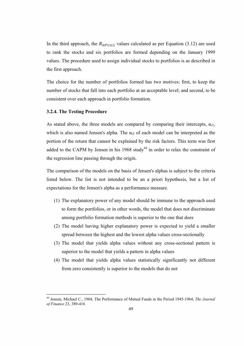
49  

In the third approach, the values calculated as per Equation (3.12) are used

to rank the stocks and six portfolios are formed depending on the January 1999

values. The procedure used to assign individual stocks to portfolios is as described in

the first approach.

The choice for the number of portfolios formed has two motives; first, to keep the

number of stocks that fall into each portfolio at an acceptable level; and second, to be

consistent over each approach in portfolio formation.

3.2.4. The Testing Procedure

As stated above, the three models are compared by comparing their intercepts, αiT,

which is also named Jensen's alpha. The αiT of each model can be interpreted as the

portion of the return that cannot be explained by the risk factors. This term was first

added to the CAPM by Jensen in his 1968 study44 in order to relax the constraint of

the regression line passing through the origin.

The comparison of the models on the basis of Jensen's alphas is subject to the criteria

listed below. The list is not intended to be an a priori hypothesis, but a list of

expectations for the Jensen's alpha as a performance measure.

(1) The explanatory power of any model should be immune to the approach used

to form the portfolios, or in other words, the model that does not discriminate

among portfolio formation methods is superior to the one that does

(2) The model having higher explanatory power is expected to yield a smaller

spread between the highest and the lowest alpha values cross-sectionally

(3) The model that yields alpha values without any cross-sectional pattern is

superior to the model that yields a pattern in alpha values

(4) The model that yields alpha values statistically significantly not different

from zero consistently is superior to the models that do not

                                                            44 Jensen, Michael C., 1968, The Performance of Mutual Funds in the Period 1945-1964, The Journal of Finance 23, 389-416

50  

3.2.5. Calculation of Performance Measures

The performance measures (αiT) are calculated by regressing the monthly portfolio

returns on independent variables related to each model over the time period of

interest. The mentioned procedure is repeated for each portfolio formation approach

and for each model and the results are reported in Chapter 4. The statistical

significance of calculated αiT values are also reported.

3.2.6. Time Frame of Independent Variables and Performance Comparison

Table 3.2 below summarizes the related time periods for each independent variable

used in this study. Even though all the independent variables are calculated for the

time periods mentioned in Table 3.2, the comparison of the performance measures is

only possible between January of 1999 and December of 2010.

Table 3.2: Time Periods of Independent Variables

Total Months Beginning Month Ending Month

Single Factor β 144 January 1999 December 2010

SMB – HML 222 July 1992 December 2010

WML 240 January 1991 December 2010

51  

CHAPTER 4

RESULTS AND ANALYSIS

4.1. DETAILS ABOUT THE METHODOLOGY

4.1.1. The Numbers of Stocks Used

The total number of stocks at the beginning of the analysis is 428, which includes

stocks that have at least one end-of-the-month price between January 1990 and

December 2010. 8 of these stocks disappear after those stocks that are traded on the

watch list or corporate products or new technologies markets in a given month are

excluded from the sample. 100 out of the remaining 420 stocks are financial sector

stocks (banks, insurance companies, mutual funds, etc.) and they are also removed

from the data set. These filters leave 320 stocks in the sample for analysis.

Table 4.1 presents the number of stocks that are used to form beta-ranked portfolios

by using the Fama MacBeth method.

Table 4.1: Number of Stocks Used To Form Beta-Based Portfolios

(Beginning-of-Year Numbers)

YEAR NUMBER OF

STOCKS YEAR

NUMBER OF STOCKS

YEAR NUMBER OF

STOCKS

1999 52 2003 110 2007 166

2000 47 2004 109 2008 162

2001 42 2005 109 2009 156

2002 41 2006 109 2010 151

52  

The SMB and HML factors as well as the related portfolio returns are calculated

Following Fama and French's (1993) procedure, and the number of stocks used for

these calculations are presented in Table 4.2.

Table 4.2: Number of Stocks Used For SMB and HML Factor Calculations

YEAR NUM. OF STOCKS

YEAR NUM. OF STOCKS

YEAR NUM. OF STOCKS

YEAR NUM. OF STOCKS

1992 90 1997 169 2002 177 2007 200

1993 103 1998 190 2003 182 2008 198

1994 115 1999 193 2004 192 2009 208

1995 138 2000 185 2005 202 2010 210

1996 153 2001 197 2006 201

Following Carhart's procedure, the past 11-month compound returns are used to rank

stocks and form momentum-based portfolios in order to calculate the WML factor.

The numbers of stocks that are used in these calculations are given in Table 4.3 as of

January of related year.

Table 4.3: Number of Stocks Used to Form Momentum Based-Portfolios

(As of January of Corresponding Year)

YEAR NUM. OF STOCKS

YEAR NUM. OF STOCKS

YEAR NUM. OF STOCKS

YEAR NUM. OF STOCKS

1991 60 1996 148 2001 193 2006 230

1992 85 1997 165 2002 217 2007 225

1993 101 1998 182 2003 216 2008 228

1994 111 1999 197 2004 219 2009 224

1995 131 2000 200 2005 223 2010 218

53  

4.1.2. Remarks About Book-to-Market Equity Based Portfolio Formation

All calculations carried out in this study are based on the same price data set. The

adjusted end-of-month prices are multiplied by the number of shares outstanding in

order to calculate the market values of stocks. The adjustment procedure of the price

reflects not only the splits and dividends, but also the changes in the value of the

Turkish Lira (the division by 1,000,000 at the beginning of 2005).

The methodology presented in Chapter 3 explains the procedure for sorting stocks

depending on their book-to-market equity values. Grouping stocks in such a manner,

builds portfolios that have an unbalanced number of stocks cross-sectionally. For

instance, such a classification for year 1991 leaves only 1 stock in the "high BE/ME"

portfolio while 89 stocks are placed into the "low BE/ME" portfolio, with zero stocks

in the "medium BE/ME" portfolio.

This problem is overcome by grouping stocks based on the number of eligible stocks.

Following the descending sort of stocks based on their BE/ME ratio value, top 30%

of the stocks are labeled with H (for High BE/ME), bottom 30% are labeled L (for

Low BE/ME) and the rest are labeled M (for Middle BE/ME). Due to the need for

using integer numbers in grouping stocks in portfolios, the number of eligible stocks

times 0.3 is rounded up to the nearest integer regardless of the magnitude of the

decimal part.

4.1.3. The Time Frame of Regressions

This study uses three different approaches to form 6 portfolios per approach. The

summary statistics of the portfolio returns are reported in Table 4.4. As a result, a

total of 18 time-series portfolio returns are regressed on the independent variables of

the excess market return (MR-RF) and the small minus big (SMB), high minus low

(HML), and winner minus loser (WML) factors in different combinations depending

on the model employed. The summary statistics about the independent variables are

reported in Table 4.5.

54  

 

STATISTIC P1-RF P2-RF P3-RF P4-RF P5-RF P6-RFCOUNT 144 144 144 144 144 144MINIMUM -0.4298 -0.4284 -0.4563 -0.5107 -0.4498 -0.4175MAXIMUM 0.7414 0.7814 0.6944 1.0780 0.5945 0.6569MEAN 0.0148 0.0165 0.0095 0.0142 0.0134 0.0164STANDARD DEVIATION 0.1515 0.1452 0.1452 0.1578 0.1399 0.1421t-STATISTIC (for the mean) 1.1713 1.3658 0.7821 1.0796 1.1466 1.3819AUTOCORRELATIONLAG 1 MONTH 0.0683 0.0625 0.0477 0.0982 0.0292 0.0199LAG 2 MONTHS -0.0452 -0.0029 -0.0239 -0.0314 0.0763 -0.0376LAG 12 MONTHS 0.0540 -0.0416 -0.0094 -0.0457 -0.0090 0.0682

STATISTIC BH-RF BM-RF BL-RF SH-RF SM-RF SL-RFCOUNT 144 144 144 144 144 144MINIMUM -0.3809 -0.4529 -0.4145 -0.4617 -0.4647 -0.5036MAXIMUM 1.0183 0.6381 0.6185 2.5735 0.4925 0.6244MEAN 0.0079 0.0067 0.0041 0.0490 0.0088 0.0099STANDARD DEVIATION 0.1396 0.1368 0.1361 0.3317 0.1266 0.1459t-STATISTIC (for the mean) 0.6790 0.5917 0.3631 1.7718 0.8297 0.8109AUTOCORRELATIONLAG 1 MONTH 0.0252 0.0639 -0.0016 -0.0561 0.0478 0.0211LAG 2 MONTHS 0.0018 0.0177 0.0177 -0.0187 -0.0196 -0.0337LAG 12 MONTHS 0.0399 0.0207 -0.0105 -0.0165 0.0254 0.0334

STATISTIC P1-RF P2-RF P3-RF P4-RF P5-RF P6-RFCOUNT 144 144 144 144 144 144MINIMUM -0.5005 -0.4774 -0.4034 -0.4616 -0.4303 -0.4636MAXIMUM 0.4956 0.6375 0.6905 0.7262 0.7736 0.9356MEAN 0.0055 0.0096 0.0160 0.0147 0.0145 0.0180STANDARD DEVIATION 0.1192 0.1296 0.1319 0.1429 0.1501 0.1691t-STATISTIC (for the mean) 0.5560 0.8920 1.4512 1.2303 1.1621 1.2786AUTOCORRELATIONLAG 1 MONTH 0.0289 0.0489 0.0922 0.1144 0.0903 0.1262LAG 2 MONTHS 0.0488 0.0213 0.0216 -0.0077 -0.0815 -0.0877LAG 12 MONTHS -0.0138 -0.0327 -0.0343 -0.0274 0.0309 0.0004

BETA PORTFOLIOS

SIZE & BOOK-TO-MARKET VALUE PORTFOLIOS

MOMENTUM PORTFOLIOS

Table 4.4: Summary Statistics for Dependent Variables

55  

The three different methods to calculate the factors and to form the portfolios

produce results for different time intervals as described in Table 3.2. Since the

purpose of this study is to compare models on the basis of different portfolio

formation approaches, it is considered as an important issue to keep the time frame

constant throughout the study. Even though all the factors and portfolio returns are

available for the time intervals beginning in 1990, this study reports results from the

January 1999 - December 2010 period in order to provide comparable model

estimates.

4.2. RESULTS

The adjusted R2's, intercepts and factor loadings are reported in Table 4.6 with the

related t-statistics in parenthesis below each value.

The adjusted R2 values of the 54 models range between 0.1224 and 0.9315 with a

mean value of 0.7870. The lowest four adjusted R2 values appear in the size and

book-to-market equity sorted portfolios modeled with the single factor. As new

STATISTIC MR-RF SMB HML WMLCOUNT 144 144 144 144MINIMUM -0.4290 -0.1914 -0.2942 -0.2935MAXIMUM 0.7557 0.8300 1.1422 0.1087MEAN 0.0072 0.0163 0.0214 -0.0104STANDARD DEVIATION 0.1455 0.1088 0.1574 0.0670t-STATISTIC (for the mean) 0.5952 1.7956 1.6348 -1.8567AUTOCORRELATIONLAG 1 MONTH -0.0358 -0.1539 -0.1888 0.2330LAG 2 MONTHS -0.0050 0.0909 -0.0199 -0.1247LAG 12 MONTHS 0.0773 -0.0112 0.0091 0.2164CORRELATIONSMR-RF 1.0000SMB -0.0940 1.0000HML 0.0997 0.7603 1.0000WML -0.4942 0.1618 0.1049 1.0000

Table 4.5: Summary Statistics for Independent Variables

56  

independent variables are introduced into the model, the adjusted R2 value increases

in all cases.

The average adjusted R2 value for the single-, three-, and, four-factor models are

0.7198, 0.8110 and 0.8304, respectively. When the SMB and HML factors are

included in the models, the increase in the explained portion of the variation in

returns is 9.12%, on average. When the WML factor is added into the three-factor

model, the explained variation increases by 1.94%, on average. There are no cross-

sectionally observable patterns in the explanatory power of the models and this

implies that none of the models differentiates between the portfolio formation

methodologies.

The intercept values consistently appear to be statistically insignificant, regardless of

what model is employed and how the portfolios are formed. The consistent

insignificance of the intercepts implies that most of the variation in the returns is

captured by the factors already included in the models.

The factor loadings of the excess market return range from 0.6986 to 1.4017 and

consistently have very high t-statistics. The overall average factor loading is 0.8632

and the average factor loading are 0.8744, 0.8905, and 0.8248 for the single-, three-

and four-factor models, respectively. It is observed that the excess market return

factor loadings for the three-factor model are consistently higher than those of the

single-factor and four-factor model estimations. The decrease in the average factor

loading of the excess market return with the introduction of the WML factor into the

model is attributed to the statistically significant factor loadings of WML; however,

the average 1.61% increase in this factor loading with the inclusion of the SMB and

HML factors is not consistent with the findings of Fama and French (1993).45

                                                            45 The average excess market return factor loading for the single-factor model, reported in Table 4 on p.20, is 1.1040, and the same average for the three-factor model, reported in Table 6 on p.24, is 1.0288. FF argue that there is a "collapse of βs for stocks toward 1.0" when SMB and HML are added to the regressions. The findings of this study are mostly consistent with this observation but the explanation of this tendency in this study does not match the explanation provided in the FF study. The SMB and HML factors in this study are highly correlated (0.7603) whereas the HML and SMB factors in the FF study are largely uncorrelated (-0.08). Fama French (1993), p.26

 

  

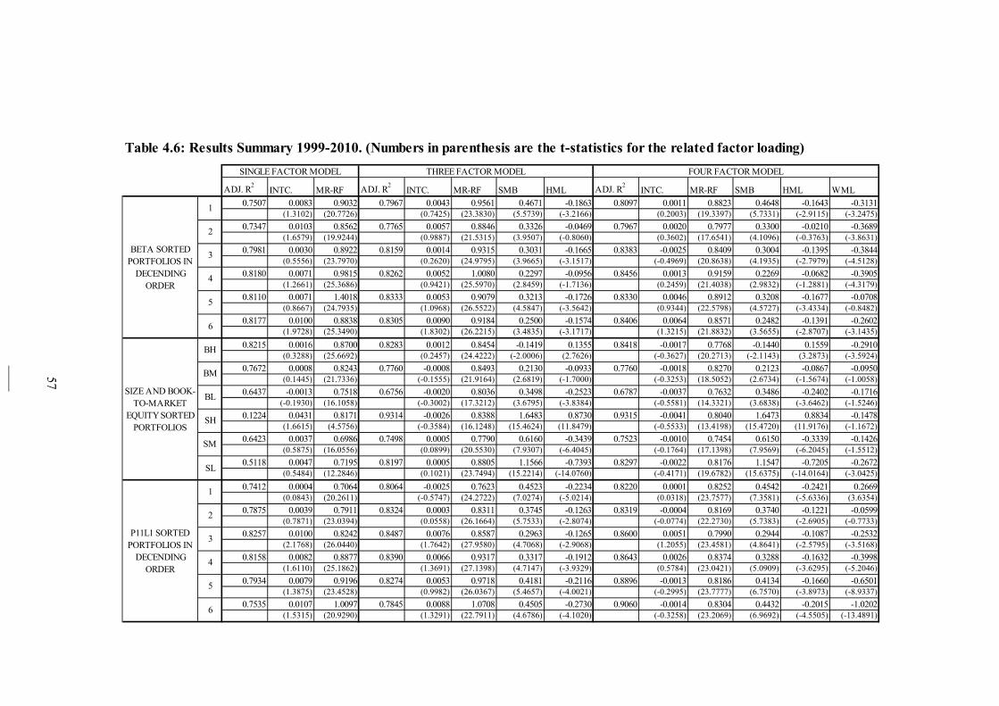
57

 

ADJ. R2

INTC. MR-RF ADJ. R2

INTC. MR-RF SMB HML ADJ. R2

INTC. MR-RF SMB HML WML0.7507 0.0083 0.9032 0.7967 0.0043 0.9561 0.4671 -0.1863 0.8097 0.0011 0.8823 0.4648 -0.1643 -0.3131

(1.3102) (20.7726) (0.7425) (23.3830) (5.5739) (-3.2166) (0.2003) (19.3397) (5.7331) (-2.9115) (-3.2475)

0.7347 0.0103 0.8562 0.7765 0.0057 0.8846 0.3326 -0.0469 0.7967 0.0020 0.7977 0.3300 -0.0210 -0.3689(1.6579) (19.9244) (0.9887) (21.5315) (3.9507) (-0.8060) (0.3602) (17.6541) (4.1096) (-0.3763) (-3.8631)

0.7981 0.0030 0.8922 0.8159 0.0014 0.9315 0.3031 -0.1665 0.8383 -0.0025 0.8409 0.3004 -0.1395 -0.3844(0.5556) (23.7970) (0.2620) (24.9795) (3.9665) (-3.1517) (-0.4969) (20.8638) (4.1935) (-2.7979) (-4.5128)

0.8180 0.0071 0.9815 0.8262 0.0052 1.0080 0.2297 -0.0956 0.8456 0.0013 0.9159 0.2269 -0.0682 -0.3905(1.2661) (25.3686) (0.9421) (25.5970) (2.8459) (-1.7136) (0.2459) (21.4038) (2.9832) (-1.2881) (-4.3179)

0.8110 0.0071 1.4018 0.8333 0.0053 0.9079 0.3213 -0.1726 0.8330 0.0046 0.8912 0.3208 -0.1677 -0.0708(0.8667) (24.7935) (1.0968) (26.5522) (4.5847) (-3.5642) (0.9344) (22.5798) (4.5727) (-3.4334) (-0.8482)

0.8177 0.0100 0.8838 0.8305 0.0090 0.9184 0.2500 -0.1574 0.8406 0.0064 0.8571 0.2482 -0.1391 -0.2602(1.9728) (25.3490) (1.8302) (26.2215) (3.4835) (-3.1717) (1.3215) (21.8832) (3.5655) (-2.8707) (-3.1435)

0.8215 0.0016 0.8700 0.8283 0.0012 0.8454 -0.1419 0.1355 0.8418 -0.0017 0.7768 -0.1440 0.1559 -0.2910(0.3288) (25.6692) (0.2457) (24.4222) (-2.0006) (2.7626) (-0.3627) (20.2713) (-2.1143) (3.2873) (-3.5924)

0.7672 0.0008 0.8243 0.7760 -0.0008 0.8493 0.2130 -0.0933 0.7760 -0.0018 0.8270 0.2123 -0.0867 -0.0950(0.1445) (21.7336) (-0.1555) (21.9164) (2.6819) (-1.7000) (-0.3253) (18.5052) (2.6734) (-1.5674) (-1.0058)

0.6437 -0.0013 0.7518 0.6756 -0.0020 0.8036 0.3498 -0.2523 0.6787 -0.0037 0.7632 0.3486 -0.2402 -0.1716(-0.1930) (16.1058) (-0.3002) (17.3212) (3.6795) (-3.8384) (-0.5581) (14.3321) (3.6838) (-3.6462) (-1.5246)

0.1224 0.0431 0.8171 0.9314 -0.0026 0.8388 1.6483 0.8730 0.9315 -0.0041 0.8040 1.6473 0.8834 -0.1478(1.6615) (4.5756) (-0.3584) (16.1248) (15.4624) (11.8479) (-0.5533) (13.4198) (15.4720) (11.9176) (-1.1672)

0.6423 0.0037 0.6986 0.7498 0.0005 0.7790 0.6160 -0.3439 0.7523 -0.0010 0.7454 0.6150 -0.3339 -0.1426(0.5875) (16.0556) (0.0899) (20.5530) (7.9307) (-6.4045) (-0.1764) (17.1398) (7.9569) (-6.2045) (-1.5512)

0.5118 0.0047 0.7195 0.8197 0.0005 0.8805 1.1566 -0.7393 0.8297 -0.0022 0.8176 1.1547 -0.7205 -0.2672(0.5484) (12.2846) (0.1021) (23.7494) (15.2214) (-14.0760) (-0.4171) (19.6782) (15.6375) (-14.0164) (-3.0425)

0.7412 0.0004 0.7064 0.8064 -0.0025 0.7623 0.4523 -0.2234 0.8220 0.0001 0.8252 0.4542 -0.2421 0.2669(0.0843) (20.2611) (-0.5747) (24.2722) (7.0274) (-5.0214) (0.0318) (23.7577) (7.3581) (-5.6336) (3.6354)

0.7875 0.0039 0.7911 0.8324 0.0003 0.8311 0.3745 -0.1263 0.8319 -0.0004 0.8169 0.3740 -0.1221 -0.0599(0.7871) (23.0394) (0.0558) (26.1664) (5.7533) (-2.8074) (-0.0774) (22.2730) (5.7383) (-2.6905) (-0.7733)

0.8257 0.0100 0.8242 0.8487 0.0076 0.8587 0.2963 -0.1265 0.8600 0.0051 0.7990 0.2944 -0.1087 -0.2532(2.1768) (26.0440) (1.7642) (27.9580) (4.7068) (-2.9068) (1.2055) (23.4581) (4.8641) (-2.5795) (-3.5168)

0.8158 0.0082 0.8877 0.8390 0.0066 0.9317 0.3317 -0.1912 0.8643 0.0026 0.8374 0.3288 -0.1632 -0.3998(1.6110) (25.1862) (1.3691) (27.1398) (4.7147) (-3.9329) (0.5784) (23.0421) (5.0909) (-3.6295) (-5.2046)

0.7934 0.0079 0.9196 0.8274 0.0053 0.9718 0.4181 -0.2116 0.8896 -0.0013 0.8186 0.4134 -0.1660 -0.6501(1.3875) (23.4528) (0.9982) (26.0367) (5.4657) (-4.0021) (-0.2995) (23.7777) (6.7570) (-3.8973) (-8.9337)

0.7535 0.0107 1.0097 0.7845 0.0088 1.0708 0.4505 -0.2730 0.9060 -0.0014 0.8304 0.4432 -0.2015 -1.0202(1.5315) (20.9290) (1.3291) (22.7911) (4.6786) (-4.1020) (-0.3258) (23.2069) (6.9692) (-4.5505) (-13.4891)

Table 4.6: Results Summary 1999-2010. (Numbers in parenthesis are the t-statistics for the related factor loading)

P11L1 SORTED PORTFOLIOS IN

DECENDING ORDER

1

2

3

4

5

6

SIZE AND BOOK-TO-MARKET

EQUITY SORTED PORTFOLIOS

BH

BM

BL

SH

SM

SL

SINGLE FACTOR MODEL THREE FACTOR MODEL FOUR FACTOR MODEL

BETA SORTED PORTFOLIOS IN

DECENDING ORDER

1

2

3

4

5

6

58  

The excess market return factor loadings are observed to be all positive and do not

demonstrate any noticeable variation among models or portfolio formation methods.

These estimates imply that investors trading in the Istanbul Stock Exchange require a

risk premium in return for the perceived riskiness in the market. This result provides

evidence in line with the previous findings in the literature. Past studies show that

even when the additional factors of SMB, HML and/or WML are included in the

models, the excess market return maintains its statistical significance. For the

Istanbul Stock Exchange case, it also seems like investors continue to price the

market-wide systematic risk significantly even when the other risk factors are

included in the models.

The Small Minus Big (SMB) factor loadings range from -0.1440 to 1.6483 with a

mean value of 0.4473 and are consistently statistically significantly different from

zero. Even though the factor loadings have varying signs, majority of them are

positive. The magnitudes of the factor loadings do not demonstrate any pattern across

portfolio formation methods and they are observed to be very close to each other in

value for the three and four-factor models. The positive factor loadings imply that the

smaller the size of the company, the larger the required rate of return by investors in

the Istanbul Stock Exchange. This evidence in support of a size risk premium is in

line with the previous findings in the literature.

The High Minus Low (HML) factor loadings are dominantly statistically

significantly different from zero (30 out of 36 observations) and have a negative sign

(32 out of 36 observations). The mean value for the factor loadings is -0.1234 with a

maximum of 0.8834 and a minimum of -0.7393. No pattern can be observed between

portfolio formation methods; however, the absolute values are smaller by 1.96% on

average for the four-factor model compared to the three-factor model.

The four positive factor loadings are observed for the high book-to-market equity

portfolios, denoted by BH and SH. These positive loadings are an indicator of the

risk premium required by the ISE investors in order to invest in financially distressed

(high BE/ME) firms. On the other hand, the predominantly negative factor loadings

for the HML factor are somewhat puzzling since they present a contradiction with

the results from earlier studies. The sign of the HML factor implies that investors in

59  

Istanbul Stock Exchange require a lower return from high book-to-market firms. In

the previous studies conducted for the developed stock markets the HML factor has a

consistently positive sign, implying a preference among investors for low BE/ME

firms.

For the Winner Minus Loser (WML) variable, in 12 out of 18 models, all but one

factor loadings are statistically significant and negative. The insignificant factor

loadings are observed when the portfolios are sorted based on size and book-to-

market equity. This observation implies a weakening of the explanatory power of the

WML factor when the portfolio formation method already accounts for the size and

book-to-market factors. No pattern in absolute values can be observed among the

different portfolio formation methods. The mostly negative coefficient estimates for

the momentum factor present another contradiction to the previous findings in the

literature. The negative factor loadings imply that investors tend to adopt a contrarian

strategy where they seem to buy past losers and sell past winners. This may also be

interpreted as evidence in support of the overreaction hypothesis where past

investment strategies are “corrected” through return reversals. The only positive

factor loading is observed for the top winner portfolio. This finding implies that,

investors seem to be interested in buying only the highest winners from the previous

11-month horizon. The highest negative factor loading is observed for the bottom

loser portfolio, and this observation is a powerful indicator of a contrarian strategy

(also, supported by the highest t-statistics). The average factor loading is -0.2789

with a maximum of 0.2669 and a minimum of -1.0202. The introduction of the factor

into the model decreases the average factor loading of the excess market return by

6.57%, and that of HML by 1.96%, while causing almost no change (0.2%) in the

SMB factor loading.

In order to investigate the possible effect of the sample period analyzed on the results

of this study, sub-period regressions are estimated for the 1999 - 2002, 2003 - 2006,

and 2007 - 2010 intervals. The estimation results are presented in Tables A.1, A.2,

and A.3 in Appendix A. The sub-period observations are in line with the

observations from the entire sample estimations. The average adjusted R2 for the

three sub-periods is 0.7494 (0.8484 for 1999 - 2002, 0.7150 for 2003 - 2006, and

60  

0.6848 for 2007 - 2010) and the adjusted R2 values consistently increase as new risk

factors are included in the models. The statistical insignificance of intercept terms

and the significance of the excess market return factors persist in all the sub-periods.

The SMB factor loadings for the three sub-periods are dominantly significant and

positive similar to the estimates for the entire sample period. Domination of negative

factor loadings for the HML factor persists for the examined sub-periods; however,

the number of significant factor loadings decreases considerably. Likewise, the

majority of WML factor loadings for the sub-periods continue to have negative

signs; however, the number of significant factor loadings decreases substantially, for

the later sub-periods.

4.3. ANALYSIS

The adjusted R2 values reported in Table 4.6 show that, except for the case of the

size and book-to-market equity based portfolio returns estimated with the single

factor model, the factors employed by the models capture a rather high percentage of

the variation in stock prices. There is one exception to this when the portfolios are

sorted based on the size and book-to-market equity ratios and the single-factor

regression model is estimated for the Small-High combination of these two factors.

This low adjusted R2 value increases considerably when the SMB and HML

variables are included in the model. It should also be noted that, even in this

exceptional case, the explanatory power of the excess market return does not

diminish for the stocks traded on the Istanbul Stock Exchange, and has significantly

large t-statistics.

The magnitude, sign and significance of the excess market return factor imply that

variation in individual stock prices has a very high positive correlation with the

variation in the ISE-100 index which mainly consists of high market capitalization

stocks. The aforementioned extreme case of the low adjusted R2 value is closely

related with the composition of the ISE-100 index. The SH (small market equity

stocks with high book-to-market equity ratio) portfolio has almost no stock in

common with the ISE-100 index; therefore, the market factor seems to lose its

significance in capturing the variation in this portfolio's returns. Also, as mentioned

61  

before, even the inclusion of the size-based factor (SMB) into the model does not

decrease the significance of the market factor. The significance of this factor

suggests that investors in the Istanbul Stock Exchange closely follow the general

movements of the market when making investment decisions.

The positive SMB loadings imply the pricing of the size risk in the Istanbul Stock

Exchange since the smaller the company, the higher the required return by the

investors. In addition, the negative HML loadings are considered as a sign of risk

aversion, since low BE/ME stocks are those stocks for which the investors are

willing to pay more. A high BE/ME ratio is regarded as a sign of financial distress.

The negative HML factor loadings finding is in contradiction with the evidence in

the Fama French 1993 paper.

The first part of Table 6 in the Fama-French 199346 paper reports insignificant

intercepts, all positive and close to 1 excess market return factor loadings, and

dominantly positive and varying magnitude SMB and HML factor loadings.

However, in their 1995 study, Fama and French provide evidence that strong,

successful firms that have strong earnings performance tend to have negative HML

loadings. They argue that the size and book-to-market risk factors are priced in the

market because they are used by investors as proxies of earnings changes that

directly result from these two risks. In general, the HML factor reflects the return

differential between value (high BE/ME) and growth (low BE/ME) stocks. If

investors in a market mostly favor value stocks, the loading on the HML should be

positive. On the other hand, if investors mostly favor growth stocks, the HML

loading should be negative. The evidence presented in Table 4.4 suggests that

investors in the Istanbul Stock Exchange prefer growth stocks over value stocks. In

addition, with reference to the 1995 Fama-French findings, Istanbul Stock Exchange

investors seem to favor companies with strong earnings performance.

With the introduction of the WML factor into the models, magnitudes of the other

three factor loadings decrease in comparison with the three-factor model. The WML

mostly captures the variation previously captured by the excess market return factor.

                                                            46 Fama and French (1993), p.24

62  

The momentum based factor appears to have less to say about the return generation

mechanism hidden behind the size and book-to-market equity based portfolio

formation method. The most noticeable finding, when the findings of this study are

compared with those of Carhart's (1997)47, is that the factor loadings have opposite

signs. The Carhart factor loadings for WML (a.k.a. PR1YR) are dominantly positive.

The sign is interpreted as the investors favoring the winners of the past 11 months.

However, the WML factor loadings of this study are dominantly negative, which can

be interpreted as a run away from the winners of past 11 months. In other words,

investors in the Istanbul Stock Exchange tend to adopt a contrarian strategy where

they seem to buy past losers and sell past winners.

Finally, the measure chosen to compare the performance of three different models

employed, Jensen's Alpha (the intercept terms of the models), consistently appears to

be statistically insignificant throughout the studied portfolios and models. Due to this

fact, it is not possible in this study to compare the performance of the models based

on the Jensen's Alpha criteria.

                                                            47 Carhart (1997), p.64, Table III

63  

CHAPTER 5

CONCLUSION

In the search for the best model that explain the return generation process of

securities traded on the Istanbul Stock Exchange, the Jensen's Alpha proved to be an

unsuitable measure for the purpose of this study. The variation in stock prices is so

dependent on the market variation that even the excess market return on its own

renders the measure useless. Therefore, this study is incapable of testing the validity

of the claims put forward in section 3.2.4. It is very important to note that the

insignificance of Jensen's Alpha, regardless of the model employed, portfolio

formation methodology applied or the time period studied, is in contrast with the

findings of earlier research. Jensen's Alpha proved to be an appropriate measure for

abnormal returns when the risk factors were unable to explain some portion of the

variation in portfolio returns. However, this study shows that in the case of Istanbul

Stock Exchange, almost all of the variation in returns is captured by the factors

already included in the models.

Despite the fact that the excess market return has about 80% explanatory power on

its own, this study shows that introduction of new risk measures into the model

brings insight about different aspects of the return generation mechanism in the

Istanbul Stock Exchange. The added factors seem to increase the total explanatory

power of the asset pricing models. Due to the consistent increase in adjusted R2

values by the addition of new explanatory variables, it is concluded that the only

measure of comparison among models can be the adjusted R2 figures. The inclusion

of the SMB and HML factors into the single factor model increases the explained

portion of variation by 9.12%. The increase attributable to the WML with the

introduction of the factor into the three-factor model is, 1.94%.

Another finding of this study which is in line with the earlier academic research is

the persistence of the significance of the excess market return factor. Earlier

64  

researchers report that regardless of the factor included in the model, the explanatory

power of the market factor does not diminish, which is confirmed by the findings of

this study as well. The continuous significance of the market factor is attributed to

the considerable pricing of systematic risk by the ISE investors.

The comparison of the outcomes of this study with the results of the earlier and well

known studies, suggests that the ISE investors do not favor high book-to-market

equity and past 11 months' winner stocks, in contrast to their US counterparts. This

finding is solely attributed to the differences between behavioral factors and / or

cultural features and requires further research.

This study follow the methodology put forward by the earlier researchers without

any fine tuning for the unique features of the market studied. However some of the

contrasting findings might have roots in the methodology applied. The time frame

used to calculate the WML factor is an example. The choice of 11 months by Carhart

(1997) is based on the findings of Jagadeesh and Titman (1993) who report 3- to 12-

month time horizons for momentum effect. The applicable time horizon for similar

effects in the ISE may prove to be a good starting point for fine tuning.

65  

REFERENCES

Banz, Rolf W., 1981, The Relationship Between Return and Market Value of

Common Stocks, Journal of Financial Economics 9, 3-18

Basu, Sanjoy, 1983, The Relationship Between Earnings Yield, Market Value, and

Return for NYSE Common Stocks: Further Evidence, Journal of Financial

Economics 12, 129-156

Berry, Michael A., Edwin Burmeister, and Marjorie B. McElroy, 1988, Sorting Out

Risks Using Known APT Factors, Financial Analysts Journal 44, 29-42

Bhandari, Laxmi Chand, 1988, Debt/Equity Ratio and Expected common Stock

Returns: Empirical Evidence, Journal of Finance 43, 507-528

Black, Fischer, 1972, Capital Market Equilibrium With Restricted Borrowing, The

Journal of Business 45, 444-455

Black, Fischer, Michael C. Jensen, and Myron Scholes, 1972, The Capital Asset

Pricing Model: Some Empirical Tests in Michael C. Jensen, ed.: Studies in the

Theory of Capital Markets (Praeger Publishers Inc.)

Bollen, Nicolas P. B., Jeffrey A. Busse, 2005, Short-Term Persistence in Mutual

Fund Performance, The Review of Financial Studies 18, 569-597

Byun, Jinho, and Michael S. Rozeff, 2003, Long-Run Performance after Stock

Splitz: 1927 to 1996, The Journal of Finance 58, 1063-1085

Carhart, Mark M., 1997, On Persistence in Mutual Fund Performance, The Journal of

Finance 52, 57-82

Chan, Louis K., Yasushi Hamao, and Josef Lakonishok, 1991, Fundamentals and

Stock Returns in Japan, Journal of Finance 46, 1739-1789

66  

Chen, Nai-Fu, Richard Roll, and Stephen A. Ross, 1986, Economic Forces and the

Stock Market, The Journal of Business 59, 383-403

Daniel, Kent, Mark Grinblatt, Sheridan Titman, and Russ Wermers, 1997, Measuring

Mutual Fund Performance with Characteristic-Based Benchmarks, The Journal of

Finance 52, 1035-1058

De Bondt, Werner F.M. and Richard Thaler, 1985, Does the Stock Market

Overreact?, The Journal of Finance 40, 793-805

De Bondt, Werner F. M. and Richard Thaler,1987, Further Evidence on Investor

Overreaction and Stock Market Seasonality, The Journal of Finance 42, 557-581

Dybvig, Philip H., and Stephen A. Ross, 1985, Yes, The APT Is Testable, The

Journal of Finance 40, 1173-1188

Fama, Eugene F. and Kenneth R. French, 1992, The Cross-Section of Expected

Stock Returns, The Journal of Finance 47, 427-465

Fama, Eugene F. and Kenneth R. French, 1993, Common Risk Factors In The

Returns On Stocks and Bonds, Journal of Financial Economics 33, 3-56

Fama, Eugene F. and Kenneth R. French, 1995, Size and Book-to-Market Factors in

Earnings and Returns, The Journal of Finance 50, 131-155

Fama, Eugene F., and Kenneth R. French, 1996, Multifactor Explanations of Asset

Pricing Anomalies, The Journal of Finance 51, 55-84

Fama, Eugene F., and James D. MacBeth, 1973, Risk, Return, and Equilibrium:

Empirical Tests, The Journal of Political Economy 81, 607-636

Fried, Irwin, and Marshall Blume, 1970, Measurement of Portfolio Performance

Under Uncertainty, American Economic Review 60, 561-575

Gibbons, Michael R., Stephen A. Ross, and Jay Shanken, 1989, A Test of the

Efficiency of a Given Portfolio, Econometrica 57, 1121-1152

67  

Gilovich, Thomas, Robert Vallone, and Amos Tversky, 1985, The Hot Hand in

Basketball: On the Misperception of Random Sequences, Cognitive Psychology 17,

295-314

Jaffe, Jeffrey, Donald B. Keim, and Randolph Westerfield, 1989, Earnings Yields,

Market Values, and Stock Returns, Journal of Finance 44, 135-148

Jagadeesh, Narasimhan, and Sheridan Titman, 1993, Returns to Buying Winners and

Selling Losers: Implications for Stock Market Efficiency, The Journal of Finance 48,

65-91

Jensen, Michael C., 1968, The Performance of Mutual Funds in the Period 1945-

1964, The Journal of Finance 23, 389-416

Kallberg, Jarl G., Crocker L. Liu, and Charles Trzcinka, 2000, The Value Added

from Investment Managers: An Examination of Funds of REITs, The Journal of

Financial and Quantitative Analysis 35, 387-408

Kothari, S. P., and Jerold B. Werner, 2001, Evaluating Mutual Fund Performance,

The Journal of Finance 56, 1985-2010

Lakonishok, Josef, Andrei Shleifer, and Robert W. Vishny, 1994, Contrarian

Investment, Extrapolation, and risk, Journal of Finance 49, 1541-1578

Lintner, John, 1965, The Valuation of Risk Assets and the Selection of Risky

Investments in Stock Portfolios and Capital Budgets, The Review of Economics and

Statistics 47, 13-37

Miller, Merton H., and Myron Scholes, 1972, Rates of Return In Relation To Risk: A

Re-Examination of Some Recent Findings, in Michael C. Jensen, ed.: Studies in the

Theory of Capital Markets (Praeger Publishers Inc.)

Markowitz, Harry, 1952, Portfolio Selection, The Journal of Finance 7, 77-91

Moskowitz, Tobias J., and Mark Grinblatt, 1999, Do Industries Explain Momentum?,

The Journal of Finance 54, 1249-1290

68  

Moskowitz, Tobias J., 2003, An Analysis of Covariance Risk and Pricing Anomalies,

The Review of Financial Studies 16, 417-457

Mossin, Jan, 1966, Equilibrium in a Capital Asset Market, Econometrica 34, 768-

783

Pratt, Shannon P., 1967, Relationship Between Viability of Past Returns and Levels

of Future Returns For Common Stocks, 1926-1960, Memorandum

Roll, Richard, and Stephen A. Ross, 1980, An Empirical Investigation of the

Arbitrage Pricing Theory, The Journal of Finance 35, 1073-1103

Rosenberg, Barr, Kenneth Reid, and Donald Lanstein, 1985, Persuasive Evidence of

Market Inefficiency, Journal of Portfolio Management 11, 9-17

Ross, Stephen A., 1976, The Arbitrage Theory of Capital Asset Pricing, Journal of

Economic Theory 13, 341-360

Shanken, Jay, 1982, The Arbitrage Pricing Theory: Is it Testable?, The Journal of

Finance 37, 1129-1140

Shanken, Jay, 1985, Multivariate Tests of the Zero-Beta CAPM, Journal of

Financial Economics 14, 327-348

Sharpe, William F., 1964, Capital Asset Prices: A Theory of Market Equilibrium

Under Conditions of Risk, The Journal of Finance 19, 425-442

Stattman, Bennis, 1980, Book Values and Stock Returns, The Chicago MBA: A

Journal of Selected Papers 4, 25-45

Tobin, James, 1958, Liquidity Preference As Behavior Towards Risk, The Review of

Economic Studies 25, 65-86

Wermers, Russ, 2000, Mutual Fund Performance: An Empirical Decomposition into

Stock-Picking Talent, Style, Transaction Costs, and Expenses, The Journal of

Finance 55, 1655-1695

69  

APPENDIX A

RESULTS SUMMARY TABLES FOR SUB-PERIOD ESTIMATIONS

 

70

ADJ. R2 INTC MR-RF ADJ. R2 INTC MR-RF SMB HML ADJ. R2 INTC MR-RF SMB HML WML0.8216 0.0071 0.9281 0.8375 0.0065 0.9923 0.3866 -0.2983 0.8726 -0.0119 0.8243 0.4334 -0.1995 -0.6189

(0.5351) (14.7457) (0.5045) (15.0529) (1.5419) (-1.4532) (-0.9570) (11.0596) (1.9496) (-1.0859) (-3.6258)0.8038 0.0026 0.8755 0.8137 -0.0012 0.9170 0.5242 0.2325 0.8362 -0.0157 0.7839 0.5613 0.3107 -0.4900

(0.1940) (13.9107) (-0.0896) (13.6264) (2.0483) (1.1095) (-1.1691) (9.7284) (2.3351) (1.5638) (-2.6548)0.8183 0.0100 0.9345 0.8404 0.0087 1.0102 0.5019 -0.2800 0.8631 -0.0066 0.8706 0.5408 -0.1980 -0.5142

(0.7368) (14.5852) (0.6748) (15.3291) (2.0025) (-1.3647) (-0.5083) (11.1688) (2.3260) (-1.0303) (-2.8804)0.8824 0.0113 1.0615 0.8981 0.0065 1.1009 0.5957 0.3725 0.9218 -0.0101 0.9490 0.6380 0.4618 -0.5593

(0.9462) (18.8059) (0.5823) (19.0903) (2.7161) (2.0746) (-0.9352) (14.7082) (3.3150) (2.9029) (-3.7848)0.8435 0.0088 0.8604 0.8574 0.0068 0.9196 0.4724 -0.0956 0.8544 0.0054 0.9063 0.4761 -0.0878 -0.0492

(0.7726) (15.9480) (0.6189) (16.2730) (2.1978) (-0.5433) (0.4394) (12.4264) (2.1883) (-0.4881) (-0.2943)0.8557 0.0168 0.9060 0.8658 0.0152 0.9610 0.4231 -0.1135 0.8686 0.0082 0.8979 0.4406 -0.0765 -0.2324

(1.4677) (16.7236) (1.3568) (16.7615) (1.9401) (-0.6360) (0.6817) (12.3963) (2.0393) (-0.4281) (-1.4010)0.8341 -0.0013 0.9167 0.8584 -0.0036 0.8738 -0.0289 0.5544 0.8888 -0.0204 0.7207 0.0138 0.6443 -0.5638

(-0.1018) (15.4060) (-0.3095) (14.4868) (-0.1260) (2.9519) (-1.7879) (10.5548) (0.0677) (3.8277) (-3.6050)0.8845 -0.0049 0.8615 0.8887 -0.0049 0.8952 0.1745 -0.2003 0.9004 -0.0149 0.8038 0.1999 -0.1466 -0.3365

(-0.5138) (18.9954) (-0.5177) (18.3234) (0.9390) (-1.3167) (-1.5145) (13.6233) (1.1360) (-1.0079) (-2.4898)0.7204 -0.0050 0.7855 0.8017 -0.0001 0.8353 -0.1427 -0.9177 0.8071 -0.0085 0.7584 -0.1213 -0.8725 -0.2833

(-0.3316) (11.0484) (-0.0083) (12.7139) (-0.5711) (-4.4861) (-0.6167) (9.1645) (-0.4912) (-4.2767) (-1.4946)0.7557 0.0071 0.7848 0.8009 0.0028 0.8751 0.8275 0.0207 0.8056 -0.0052 0.8027 0.8477 0.0632 -0.2668

(0.5203) (12.0977) (0.2217) (13.6173) (3.3855) (0.1033) (-0.3804) (9.8975) (3.5039) (0.3163) (-1.4363)0.6722 -0.0047 0.6732 0.8203 -0.0107 0.8156 1.2342 -0.0771 0.8378 -0.0217 0.7153 1.2621 -0.0181 -0.3694

(-0.3229) (9.8686) (-0.9900) (14.7144) (5.8544) (-0.4465) (-1.9290) (10.6364) (6.2915) (-0.1092) (-2.3986)0.7217 0.0018 0.7729 0.8437 -0.0008 0.9136 0.9413 -0.5073 0.8788 -0.0170 0.7649 0.9827 -0.4199 -0.5473

(0.1230) (11.0861) (-0.0677) (15.9353) (4.3170) (-2.8417) (-1.5803) (11.8639) (5.1092) (-2.6418) (-3.7061)0.8189 -0.0072 0.6931 0.9110 -0.0117 0.7974 0.9096 -0.0482 0.9104 -0.0090 0.8222 0.9027 -0.0627 0.0912

(-0.7205) (14.6126) (-1.6478) (21.8539) (6.5546) (-0.4240) (-1.1532) (17.5883) (6.4735) (-0.5442) (0.8514)0.8497 -0.0007 0.7907 0.8831 -0.0040 0.8645 0.6491 -0.0255 0.8875 -0.0106 0.8042 0.6659 0.0100 -0.2220

(-0.0711) (16.3342) (-0.4346) (18.4534) (3.6429) (-0.1747) (-1.0777) (13.7034) (3.8035) (0.0688) (-1.6520)0.8696 0.0097 0.8317 0.8799 0.0080 0.8812 0.4000 -0.0719 0.8957 -0.0031 0.7800 0.4282 -0.0124 -0.3726

(0.9811) (17.7356) (0.8310) (17.8414) (2.1293) (-0.4673) (-0.3133) (13.2690) (2.4417) (-0.0856) (-2.7673)0.8482 0.0075 0.9143 0.8750 0.0044 0.9933 0.6696 -0.0663 0.9058 -0.0122 0.8417 0.7119 0.0228 -0.5583

(0.6322) (16.2347) (0.4006) (17.7140) (3.1397) (-0.3800) (-1.1763) (13.5377) (3.8381) (0.1484) (-3.9208)0.8233 0.0155 0.9458 0.8597 0.0125 1.0415 0.7435 -0.1853 0.9287 -0.0130 0.8084 0.8085 -0.0484 -0.8584

(1.1496) (14.8334) (1.0298) (16.7032) (3.1352) (-0.9547) (-1.3712) (14.2420) (4.7747) (-0.3457) (-6.6030)0.8106 0.0288 1.0528 0.8346 0.0259 1.1449 0.7197 -0.1708 0.9474 -0.0105 0.8127 0.8123 0.0244 -1.2232

(1.8381) (14.2171) (1.7480) (15.0759) (2.4920) (-0.7223) (-1.1483) (14.8592) (4.9790) (0.1809) (-9.7646)

THREE FACTOR MODEL FOUR FACTOR MODEL

BETA SORTED PORTFOLIOS IN

DECENDING ORDER

1

2

3

4

5

6

Table A.1: Results Summary 1999-2002. (Numbers in paranthesis are the t-statistics for the related factor loading)

P11L1 SORTED PORTFOLIOS IN

DECENDING ORDER

1

2

3

4

5

6

SIZE AND BOOK-TO-MARKET

EQUITY SORTED PORTFOLIOS

BH

BM

BL

SH

SM

SL

SINGLE FACTOR MODEL

 

71

ADJ. R2 INTC MR-RF ADJ. R2 INTC MR-RF SMB HML ADJ. R2 INTC MR-RF SMB HML WML0.8313 0.0023 0.8104 0.8346 0.0034 0.8204 0.1416 -0.0992 0.8354 0.0040 0.8316 0.1357 -0.0900 -0.1436

(0.4517) (15.2529) (0.6767) (15.4733) (1.5906) (-1.6977) (0.7848) (15.4415) (1.5249) (-1.5298) (-1.1031)0.4991 0.0175 0.6831 0.7151 0.0112 0.6663 0.3824 -0.0328 0.7199 0.0121 0.6851 0.3724 -0.0175 -0.2416

(1.8826) (6.9157) (1.5548) (8.8775) (3.0332) (-0.3972) (1.6913) (9.0401) (2.9733) (-0.2110) (-1.3190)0.7457 0.0000 0.7828 0.7535 -0.0001 0.7889 0.1950 -0.0957 0.7728 0.0013 0.8153 0.1810 -0.0742 -0.3384

(-0.0039) (11.7832) (-0.0095) (11.9704) (1.7616) (-1.3183) (0.2065) (12.6525) (1.6999) (-1.0536) (-2.1730)0.6521 0.0039 0.7432 0.6695 0.0058 0.7604 0.2620 -0.1764 0.6874 0.0072 0.7875 0.2476 -0.1543 -0.3476

(0.5303) (9.4388) (0.7861) (9.8318) (2.0173) (-2.0705) (0.9914) (10.2831) (1.9570) (-1.8438) (-1.8781)0.7905 0.0076 0.9341 0.8075 0.0093 0.9507 0.2743 -0.1772 0.8202 0.0105 0.9760 0.2609 -0.1566 -0.3249

(1.1549) (13.3534) (1.4354) (14.0718) (2.4176) (-2.3814) (1.6788) (14.6776) (2.3742) (-2.1546) (-2.0221)0.6594 0.0034 0.7006 0.6684 0.0054 0.7159 0.1935 -0.1441 0.6896 0.0067 0.7429 0.1792 -0.1221 -0.3463

(0.4993) (9.5907) (0.7751) (9.8558) (1.5863) (-1.8009) (0.9966) (10.3824) (1.5156) (-1.5613) (-2.0029)0.8038 0.0044 0.7205 0.8104 0.0036 0.7114 -0.1621 0.1014 0.8121 0.0042 0.7230 -0.1682 0.1109 -0.1493

(0.9101) (13.9115) (0.7299) (13.8639) (-1.8807) (1.7935) (0.8480) (13.9031) (-1.9579) (1.9511) (-1.1883)0.6173 0.0025 0.7462 0.6013 0.0029 0.7466 -0.0386 0.0103 0.5967 0.0035 0.7584 -0.0449 0.0199 -0.1520

(0.3180) (8.7650) (0.3469) (8.5264) (-0.2624) (0.1065) (0.4130) (8.4574) (-0.3028) (0.2035) (-0.7012)0.6650 -0.0114 0.7335 0.6545 -0.0107 0.7398 0.0966 -0.0652 0.6874 -0.0091 0.7733 0.0789 -0.0379 -0.4292

(-1.6070) (9.7112) (-1.4502) (9.5720) (0.7443) (-0.7657) (-1.2807) (10.3298) (0.6376) (-0.4631) (-2.3727)0.0367 0.0606 0.9750 0.9730 -0.0104 0.6915 1.3225 1.0976 0.9739 -0.0089 0.7214 1.3067 1.1220 -0.3835

(1.1022) (1.6705) (-1.1025) (7.0164) (7.9903) (10.1099) (-0.9564) (7.3176) (8.0214) (10.4153) (-1.6100)0.6851 -0.0003 0.8151 0.7728 0.0023 0.8433 0.5096 -0.3154 0.7784 0.0032 0.8623 0.4995 -0.2999 -0.2433

(-0.0396) (10.1614) (0.3424) (12.2818) (4.4192) (-4.1697) (0.4903) (12.4903) (4.3790) (-3.9756) (-1.4587)0.3530 -0.0045 0.5897 0.8252 0.0039 0.6630 1.0638 -0.7358 0.8231 0.0043 0.6711 1.0596 -0.7292 -0.1036

(-0.4220) (5.1616) (0.6833) (11.0801) (10.5858) (-11.1614) (0.7456) (10.9502) (10.4627) (-10.8877) (-0.6998)0.6904 0.0000 0.8539 0.7499 -0.0007 0.8635 0.4088 -0.1831 0.7585 -0.0019 0.8408 0.4208 -0.2016 0.2910

(0.0051) (10.2859) (-0.1039) (11.4861) (3.2379) (-2.2108) (-0.2645) (11.1775) (3.3857) (-2.4525) (1.6008)0.7733 0.0076 0.7921 0.7781 0.0088 0.8034 0.1737 -0.1164 0.7732 0.0090 0.8060 0.1724 -0.1143 -0.0326

(1.2933) (12.7019) (1.4827) (12.9210) (1.6635) (-1.6994) (1.4802) (12.5908) (1.6296) (-1.6345) (-0.2106)0.7010 0.0135 0.7793 0.7332 0.0131 0.7868 0.2961 -0.1356 0.7633 0.0147 0.8194 0.2788 -0.1090 -0.4182

(1.9427) (10.5454) (1.9416) (11.1862) (2.5065) (-1.7504) (2.3061) (12.1447) (2.5008) (-1.4788) (-2.5649)0.7193 0.0076 0.7484 0.7296 0.0089 0.7611 0.2154 -0.1374 0.7526 0.0102 0.7889 0.2006 -0.1147 -0.3568

(1.1912) (11.0196) (1.3780) (11.3306) (1.9090) (-1.8562) (1.6582) (12.0589) (1.8558) (-1.6038) (-2.2567)0.6738 -0.0016 0.7546 0.6885 -0.0012 0.7648 0.2537 -0.1364 0.7657 0.0013 0.8139 0.2276 -0.0964 -0.6300

(-0.2218) (9.9036) (-0.1609) (10.1943) (2.0133) (-1.6507) (0.2071) (12.2832) (2.0789) (-1.3307) (-3.9342)0.5402 -0.0054 0.7395 0.6162 -0.0025 0.7693 0.5001 -0.3205 0.7822 0.0014 0.8464 0.4592 -0.2576 -0.9894

(-0.5818) (7.4977) (-0.2828) (8.4711) (3.2791) (-3.2037) (0.2116) (12.1525) (3.9901) (-3.3841) (-5.8783)

THREE FACTOR MODEL FOUR FACTOR MODEL

BETA SORTED PORTFOLIOS IN

DECENDING ORDER

1

2

3

4

5

6

Table A.2: Results Summary 2003 - 2006. (Numbers in paranthesis are the t-statistics for the related factor loading)

P11L1 SORTED PORTFOLIOS IN

DECENDING ORDER

1

2

3

4

5

6

SIZE AND BOOK-TO-MARKET

EQUITY SORTED PORTFOLIOS

BH

BM

BL

SH

SM

SL

SINGLE FACTOR MODEL

 

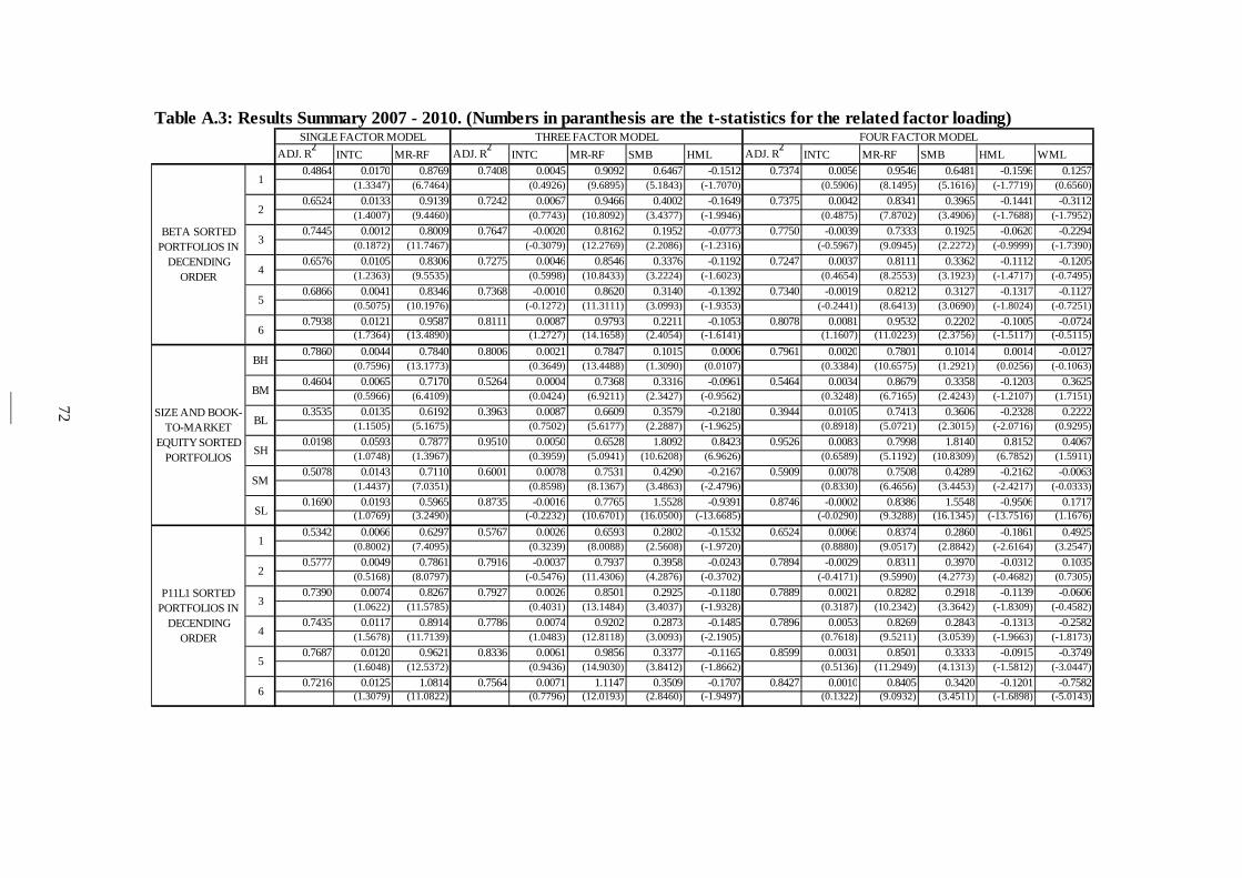
72

 

ADJ. R2 INTC MR-RF ADJ. R2 INTC MR-RF SMB HML ADJ. R2 INTC MR-RF SMB HML WML0.4864 0.0170 0.8769 0.7408 0.0045 0.9092 0.6467 -0.1512 0.7374 0.0056 0.9546 0.6481 -0.1596 0.1257

(1.3347) (6.7464) (0.4926) (9.6895) (5.1843) (-1.7070) (0.5906) (8.1495) (5.1616) (-1.7719) (0.6560)0.6524 0.0133 0.9139 0.7242 0.0067 0.9466 0.4002 -0.1649 0.7375 0.0042 0.8341 0.3965 -0.1441 -0.3112

(1.4007) (9.4460) (0.7743) (10.8092) (3.4377) (-1.9946) (0.4875) (7.8702) (3.4906) (-1.7688) (-1.7952)0.7445 0.0012 0.8009 0.7647 -0.0020 0.8162 0.1952 -0.0773 0.7750 -0.0039 0.7333 0.1925 -0.0620 -0.2294

(0.1872) (11.7467) (-0.3079) (12.2769) (2.2086) (-1.2316) (-0.5967) (9.0945) (2.2272) (-0.9999) (-1.7390)0.6576 0.0105 0.8306 0.7275 0.0046 0.8546 0.3376 -0.1192 0.7247 0.0037 0.8111 0.3362 -0.1112 -0.1205

(1.2363) (9.5535) (0.5998) (10.8433) (3.2224) (-1.6023) (0.4654) (8.2553) (3.1923) (-1.4717) (-0.7495)0.6866 0.0041 0.8346 0.7368 -0.0010 0.8620 0.3140 -0.1392 0.7340 -0.0019 0.8212 0.3127 -0.1317 -0.1127

(0.5075) (10.1976) (-0.1272) (11.3111) (3.0993) (-1.9353) (-0.2441) (8.6413) (3.0690) (-1.8024) (-0.7251)0.7938 0.0121 0.9587 0.8111 0.0087 0.9793 0.2211 -0.1053 0.8078 0.0081 0.9532 0.2202 -0.1005 -0.0724

(1.7364) (13.4890) (1.2727) (14.1658) (2.4054) (-1.6141) (1.1607) (11.0223) (2.3756) (-1.5117) (-0.5115)0.7860 0.0044 0.7840 0.8006 0.0021 0.7847 0.1015 0.0006 0.7961 0.0020 0.7801 0.1014 0.0014 -0.0127

(0.7596) (13.1773) (0.3649) (13.4488) (1.3090) (0.0107) (0.3384) (10.6575) (1.2921) (0.0256) (-0.1063)0.4604 0.0065 0.7170 0.5264 0.0004 0.7368 0.3316 -0.0961 0.5464 0.0034 0.8679 0.3358 -0.1203 0.3625

(0.5966) (6.4109) (0.0424) (6.9211) (2.3427) (-0.9562) (0.3248) (6.7165) (2.4243) (-1.2107) (1.7151)0.3535 0.0135 0.6192 0.3963 0.0087 0.6609 0.3579 -0.2180 0.3944 0.0105 0.7413 0.3606 -0.2328 0.2222

(1.1505) (5.1675) (0.7502) (5.6177) (2.2887) (-1.9625) (0.8918) (5.0721) (2.3015) (-2.0716) (0.9295)0.0198 0.0593 0.7877 0.9510 0.0050 0.6528 1.8092 0.8423 0.9526 0.0083 0.7998 1.8140 0.8152 0.4067

(1.0748) (1.3967) (0.3959) (5.0941) (10.6208) (6.9626) (0.6589) (5.1192) (10.8309) (6.7852) (1.5911)0.5078 0.0143 0.7110 0.6001 0.0078 0.7531 0.4290 -0.2167 0.5909 0.0078 0.7508 0.4289 -0.2162 -0.0063

(1.4437) (7.0351) (0.8598) (8.1367) (3.4863) (-2.4796) (0.8330) (6.4656) (3.4453) (-2.4217) (-0.0333)0.1690 0.0193 0.5965 0.8735 -0.0016 0.7765 1.5528 -0.9391 0.8746 -0.0002 0.8386 1.5548 -0.9506 0.1717

(1.0769) (3.2490) (-0.2232) (10.6701) (16.0500) (-13.6685) (-0.0290) (9.3288) (16.1345) (-13.7516) (1.1676)0.5342 0.0066 0.6297 0.5767 0.0026 0.6593 0.2802 -0.1532 0.6524 0.0066 0.8374 0.2860 -0.1861 0.4925

(0.8002) (7.4095) (0.3239) (8.0088) (2.5608) (-1.9720) (0.8880) (9.0517) (2.8842) (-2.6164) (3.2547)0.5777 0.0049 0.7861 0.7916 -0.0037 0.7937 0.3958 -0.0243 0.7894 -0.0029 0.8311 0.3970 -0.0312 0.1035

(0.5168) (8.0797) (-0.5476) (11.4306) (4.2876) (-0.3702) (-0.4171) (9.5990) (4.2773) (-0.4682) (0.7305)0.7390 0.0074 0.8267 0.7927 0.0026 0.8501 0.2925 -0.1180 0.7889 0.0021 0.8282 0.2918 -0.1139 -0.0606

(1.0622) (11.5785) (0.4031) (13.1484) (3.4037) (-1.9328) (0.3187) (10.2342) (3.3642) (-1.8309) (-0.4582)0.7435 0.0117 0.8914 0.7786 0.0074 0.9202 0.2873 -0.1485 0.7896 0.0053 0.8269 0.2843 -0.1313 -0.2582

(1.5678) (11.7139) (1.0483) (12.8118) (3.0093) (-2.1905) (0.7618) (9.5211) (3.0539) (-1.9663) (-1.8173)0.7687 0.0120 0.9621 0.8336 0.0061 0.9856 0.3377 -0.1165 0.8599 0.0031 0.8501 0.3333 -0.0915 -0.3749

(1.6048) (12.5372) (0.9436) (14.9030) (3.8412) (-1.8662) (0.5136) (11.2949) (4.1313) (-1.5812) (-3.0447)0.7216 0.0125 1.0814 0.7564 0.0071 1.1147 0.3509 -0.1707 0.8427 0.0010 0.8405 0.3420 -0.1201 -0.7582

(1.3079) (11.0822) (0.7796) (12.0193) (2.8460) (-1.9497) (0.1322) (9.0932) (3.4511) (-1.6898) (-5.0143)

THREE FACTOR MODEL FOUR FACTOR MODEL

BETA SORTED PORTFOLIOS IN

DECENDING ORDER

1

2

3

4

5

6

Table A.3: Results Summary 2007 - 2010. (Numbers in paranthesis are the t-statistics for the related factor loading)

P11L1 SORTED PORTFOLIOS IN

DECENDING ORDER

1

2

3

4

5

6

SIZE AND BOOK-TO-MARKET

EQUITY SORTED PORTFOLIOS

BH

BM

BL

SH

SM

SL

SINGLE FACTOR MODEL

 

73  

APPENDIX B: TEZ FOTOKOPİ İZİN FORMU

ENSTİTÜ

Fen Bilimleri Enstitüsü

Sosyal Bilimler Enstitüsü

Uygulamalı Matematik Enstitüsü

Enformatik Enstitüsü

Deniz Bilimleri Enstitüsü

YAZARIN

Soyadı : Kalaç

Adı : Sırrı Selim

Bölümü : İşletme

TEZİN ADI (İngilizce) : A TEST OF MULTI-INDEX ASSET PRICING MODELS: THE CASE OF ISTANBUL STOCK EXCHANGE

TEZİN TÜRÜ : Yüksek Lisans Doktora

1. Tezimin tamamı dünya çapında erişime açılsın ve kaynak gösterilmek şartıyla tezimin bir kısmı veya tamamının fotokopisi alınsın.

2. Tezimin tamamı yalnızca Orta Doğu Teknik Üniversitesi kullancılarının erişimine açılsın. (Bu seçenekle tezinizin fotokopisi ya da elektronik kopyası Kütüphane aracılığı ile ODTÜ dışına dağıtılmayacaktır.)

3. Tezim bir (1) yıl süreyle erişime kapalı olsun. (Bu seçenekle tezinizin fotokopisi ya da elektronik kopyası Kütüphane aracılığı ile ODTÜ dışına dağıtılmayacaktır.)

Yazarın imzası ............................ Tarih .............................