arX

iv:1

307.

4181

v2 [

astr

o-ph

.CO

] 25

Nov

201

4

Mon. Not. R. Astron. Soc.000, 1–16 (2013) Printed 13 February 2018 (MN LATEX style file v2.2)

A test of the Suyama-Yamaguchi inequality from weak lensing

Alessandra Grassi1⋆, Lavinia Heisenberg2,3, Christian T. Byrnes4, Bjorn Malte Schafer11Astronomisches Recheninstitut, Zentrum fur Astronomie,Universitat Heidelberg, Philosophenweg 12, 69120 Heidelberg, Germany2Departement de Physique Theorique and Center for Astroparticle Physics, Universite de Geneve, 24 Quai E. Ansermet, CH-1211, Geneve, Switzerland3Department of Physics, Case Western Reserve University, 10900 Euclid Ave, Cleveland, OH 44106, United States of America4Department of Physics and Astronomy, University of Sussex,Brighton, BN1 9RH, United Kingdom

13 February 2018

ABSTRACTWe investigate the weak lensing signature of primordial non-Gaussianities of the local typeby constraining the magnitude of the weak convergence bi- and trispectra expected for theEuclid weak lensing survey. Starting from expressions for the weak convergence spectra, bis-pectra and trispectra, whose relative magnitudes we investigate as a function of scale, wecompute their respective signal to noise ratios by relatingthe polyspectra’s amplitude to theirGaussian covariance using a Monte-Carlo technique for carrying out the configuration spaceintegrations. In computing the Fisher-matrix on the non-Gaussianity parametersfNL , gNL andτNL with a very similar technique, we can derive Bayesian evidences for a violation of theSuyama-Yamaguchi relationτNL > (6 fNL/5)2 as a function of the truefNL andτNL-valuesand show that the relation can be probed down to levels offNL ≃ 102 andτNL ≃ 105. In arelated study, we derive analytical expressions for the probability density that the SY-relationis exactly fulfilled, as required by models in which any one field generates the perturbations.We conclude with an outlook on the levels of non-Gaussianitythat can be probed with tomo-graphic lensing surveys.

Key words: cosmology: large-scale structure, gravitational lensing, methods: analytical

1 INTRODUCTION

Advances in observational cosmology has made it possible toprobe models of the early Universe and the mechanisms that can generate smallseed perturbations in the density field from which the cosmiclarge-scale structure grew by gravitational instability.One of the most prominentof these models is inflation, in which the Universe underwentan extremely rapid exponential expansion and where small fluctuations in theinflationary field gave rise to fluctuations in the gravitational potential and which then imprinted these fluctuations onto all cosmic fluids (forreviews, seeBartolo et al. 2004; Seery et al. 2007; Komatsu et al. 2009; Komatsu 2010; Desjacques & Seljak 2010b,a; Verde 2010; Jeonget al. 2011a; Wang 2013; Martin et al. 2013; Lesgourgues 2013). Observationally, inflationary models can be distinguished by the spectralindex ns along with a possible scale dependence, the scalar to tensor-ratio r and, perhaps most importantly, the non-Gaussian signatures,quantified byn-point correlation functions or by polyspectra of ordern in Fourier-space. They are of particular interest as there is a relationbetween the statistical properties of the fields and its dynamics. Additionally, the configuration space dependence of the polyspectra yieldsvaluable information on the type of inflationary model (Byun & Bean 2013).

The (possibly non-Gaussian) density fluctuations are subsequently imprinted in the cosmic microwave background (CMB)as tempera-ture anisotropies (Fergusson & Shellard 2009; Fergusson & Shellard 2007; Vielva & Sanz 2009; Fergusson et al. 2010; Pettinari et al. 2013),in the matter distribution which can be probed by e.g. gravitational lensing and in the number density of galaxies. Hereby it is advantageousthat the observable is linear in the field whose statistical property we investigate. In case of linear dependence then-point functions of theobservable field can be mapped directly onto the corresponding n-point function of the primordial density perturbation, which reflects themicrophysics of the early Universe.

The first important measurement quantifying non-Gaussianity is the parameterfNL which describes the skewness of inflationary fluc-tuations and determines the amplitude of the bispectrum. Not only the bispectrum but also the trispectrum can successfully be constrainedby future precisions measurements, where the parametersgNL andτNL determine the trispectrum amplitude. The complementary analysis ofboth the bi- and the trispectra in the future experiments will make us able to extract more information about the mechanism of generatingthe primordial curvature perturbations and constrain the model of the early Universe. Therefore, it is an indispensable task for cosmology toobtain the configuration space dependence for the higher polyspectra and to make clear predictions for the non-Gaussianity parameters. The

⋆ e-mail: sandri@ari.uni-heidelberg.de

c© 2013 RAS

2 A. Grassi, L. Heisenberg, C.T. Byrnes, B.M. Schafer

non-Gaussianities are commonly expressed as perturbations of modes of the potential∝ kns/2−2 but can in principle have scale dependences(Chen 2005; Lo Verde et al. 2008; Sefusatti et al. 2009; Riotto & Sloth 2011; Byrnes et al. 2010; Becker et al. 2011; Byrnes et al. 2010).

The first cosmological data release of the Planck satellite has resulted in the tighest ever constraints onfNL andτNL (Planck Collaborationet al. 2013a). For the local bispectrum,fNL = 2.7± 5.8, with the 1σ confidence level quoted, while the 95% upper bound on the trispectrumparameter isτNL 6 2800. ThefNL is about a factor of 4 improvement over the WMAP bound (Bennett et al. 2012; Giannantonio et al. 2013),while theτNL bound is improved by about an order of magnitude (Hikage & Matsubara 2012). No Planck bound ongNL has yet been made,the tightest bound is currentlygNL = (−3.3± 2.2)× 105 from WMAP9 data (Sekiguchi & Sugiyama 2013). Previous CMB constraints weremade in (Hikage et al. 2008; Smidt et al. 2010; Fergusson et al. 2010). The bound onfNL is close to cosmic variance limited for any CMBexperiment, for the trispectrum parameters the bounds may still improve by a factor of a few, see e.g. (Smidt et al. 2010; Fergusson et al.2010; Sekiguchi & Sugiyama 2013).

An alternative way of constraining non-Gaussianities are the number density of clusters as a function of their mass, seeFedeli et al.(2011); LoVerde & Smith(2011); Enqvist et al.(2011) who show that constraints of order 102 on fNL and 108 ongNL .

In comparison to other probes, weak gravitational lensing provides weaker bounds, but non-Gaussianities have nevertheless importantimplications for weak lensing. Although the weak lensing bispectrum is by far dominated by structure formation non-Gaussianities (Takada &Jain 2003; Bernardeau et al. 2003; Takada & Jain 2004), whose observational signature has been detected at high significance, (via the quasarmagnification bias and the aperture mass skewness,Menard et al. 2003; Semboloni et al. 2011, respectively), there are a number of studiesfocusing on primordial non-Gaussianities, for example weak lensing peak counts (Marian et al. 2011), yieldingσ fNL ≃ 10 constraints onnon-Gaussianities, or topological measures of the weak lensing map, for instance the skeleton (Fedeli et al. 2011) or Minkowski functionals(Munshi et al. 2011). Direct estimation of the inflationary weak lensing bispectra is possible (Pace et al. 2011; Schafer et al. 2012) but suffersfrom the Gaussianising effect of the line of sight-integration (Jeong et al. 2011b). Similar to the weak lensing spectrum, bispectra also sufferfrom contamination by intrinsic alignments (Semboloni et al. 2008) and baryonic physics (Semboloni et al. 2011).

The description of inflationary non-Gaussianities is done in a perturbative way and for the relative magnitude of non-Gaussianities ofdifferent order the Suyama-Yamaguchi (SY) relation applies (Suyama & Yamaguchi 2008; Suyama et al. 2010a; Lewis 2011; Smith et al.2011a; Sugiyama 2012; Assassi et al. 2012; Kehagias & Riotto 2012; Beltran Almeida et al. 2013; Rodrıguez et al. 2013; Tasinato et al.2013), which in the most basic form relates the amplitudes of the bi- and of the trispectrum. Recently, it has been proposed that testing for aviolation of the SY-inequality would make it possible to distinguish between different classes of inflationary models. In this work we focuson the relation between the non-Gaussianity parametersfNL andτNL for a local model, and investigate how well the future Euclidsurvey canprobe the SY-relation: The question we address is how likelywould we believe in the SY-inequality with the inferedfNL andτNL-values. Weaccomplish this by studying the Bayesian evidence (Trotta 2007, 2008) providing support for the SY-inequality.

Models in which a single field generates the primordial curvature perturbation predict an equality between one term of the trispectrumand the bispectrum,τNL = (6 fNL/5)2 (provided that the loop corrections are not anomalously large, if they are thengNL should also beobservableTasinato et al. 2013). Violation of this consistency relation would prove that more than one light field present during inflationhad to contribute towards the primordial curvature perturbation. However a verification of the equality would not implysingle field inflation,rather that only one of the fields generated perturbations. In fact any detection of non-Gaussianity of the local form will prove that morethan one field was present during inflation, because single field inflation predicts negligible levels of local non-Gaussianity. A detection ofτNL > (6 fNL/5)2 would prove that not only that inflation was of the multi-fieldvariety, but also that multiple-fields contributed towardstheprimordial perturbations, which are the seeds which gave rise to all the structure in the universe today. Weaker forms ofthe SY-relation,τNL > (6/5 fNL)2/2, has been proposed bySugiyama et al.(2011) for multifield-inflationary models although these may havebeen refuted bySmith et al.(2011b).

A violation of the Suyama-Yamaguchi inequality would come as a big surprise, since the inequality has been proved to holdfor allmodels of inflation. Even more strongly, in the limit of an infinite volume survey it holds true simply by the definitions ofτNL and fNL ,regardless of the theory relating to the primordial perturbations. However since realistic surveys will always have a finite volume, a breakingof the inequality could occur. It remains unclear how one should interpret a breaking of the inequality, and whether any concrete scenarioscan be constructed in which this would occur. A violation maybe related to a breaking of statistical homogeneity (Smith et al. 2011a).

After a brief summary of cosmology and structure formation in Sect.2 we introduce primordial non-Gaussianities in Sect.3 along withthe SY-inequality relating the relative non-Gaussianity strengths in the polyspectra of different order. The mapping of non-Gaussianities byweak gravitational lensing is summarised in Sect.4. Then, we investigate the attainable signal to noise-ratios (Sect.5), address degeneraciesin the measurement ofgNL andτNL in (Sect.6), carry out statistical tests of the SY-inequality (Sect.7), investigate analytical distributionsof ratios of non-Gaussianity parameters (Sect.8) and quantify the Bayesian evidence for a violation of the SY-inequality from a lensingmeasurement (Sect.9). We summarise our main results in Sect.10.

The reference cosmological model used is a spatially flatwCDM cosmology with adiabatic initial perturbations for thecold dark matter.The specific parameter choices areΩm = 0.25,ns = 1,σ8 = 0.8,Ωb = 0.04. The Hubble parameter is set toh = 0.7 and the Hubble-distanceis given byc/H0 = 2996.9 Mpc/h. The dark energy equation of state is assumed to be constant with a value ofw = −0.9. We prefer towork with these values that differ slightly from the recent Planck results (Planck Collaboration et al. 2013b) because lensing prefers lowerΩm-values and largerh-values (Heymans et al. 2013). Scale-invariance forns was chosen for simplicity and should not strongly affect theconclusions as the range of angular scales probed is small and close to the normalisation scale.

The fluctuations are taken to be Gaussian perturbed with weaknon-Gaussianities of the local type, and for the weak lensing survey weconsider the case of Euclid, with a sky coverage offsky = 1/2, a median redshift of 0.9, a yield ofn = 40 galaxies/arcmin2 and a ellipticityshape noise ofσǫ = 0.3 (Amara & Refregier 2007; Refregier 2009).

c© 2013 RAS, MNRAS000, 1–16

SY-inequality and weak lensing 3

2 COSMOLOGY AND STRUCTURE FORMATION

In spatially flat dark energy cosmologies with the matter density parameterΩm, the Hubble functionH(a) = d lna/dt is given by

H2(a)

H20

=Ωm

a3+

1− Ωm

a3(1+w), (1)

for a constant dark energy equation of state-parameterw. The comoving distanceχ and scale factora are related by

χ = c∫ 1

a

daa2H(a)

, (2)

given in units of the Hubble distanceχH = c/H0. For the linear matter power spectrumP(k) which describes the Gaussian fluctuationproperties of the linearly evolving density fieldδ,

〈δ(k)δ(k′)〉 = (2π)3δD(k + k′)P(k) (3)

the ansatzP(k) ∝ knsT2(k) is chosen with the transfer functionT(k), which is well approximated by the fitting formula

T(q) =ln(1+ 2.34q)

2.34q×

[

1+ 3.89q+ (16.1q)2 + (5.46q)3 + (6.71q)4]−1/4

, (4)

for low-matter density cosmologies (Bardeen et al. 1986). The wave vectork = qΓ enters rescaled by the shape parameterΓ (Sugiyama1995),

Γ = Ωmhexp

−Ωb

1+

√2hΩm

. (5)

The fluctuation amplitude is normalised to the varianceσ28,

σ2R =

∫

k2dk2π2

W2R(k) P(k), (6)

with a Fourier-transformed spherical top-hatWR(k) = 3 j1(kR)/(kR) as the filter function operating atR= 8 Mpc/h. jℓ(x) denotes the sphericalBessel function of the first kind of orderℓ (Abramowitz & Stegun 1972). The linear growth of the density field,δ(x,a) = D+(a)δ(x, a = 1),is described by the growth functionD+(a), which is the solution to the growth equation (Turner & White 1997; Wang & Steinhardt 1998;Linder & Jenkins 2003),

d2

da2D+(a) +

1a

(

3+d ln Hd lna

)

dda

D+(a) =3

2a2Ωm(a)D+(a). (7)

From the CDM-spectrum of the density perturbation the spectrum of the Newtonian gravitational potential can be obtained

PΦ(k) =

(

3Ωm

2χ2H

)2

kns−4 T(k)2 (8)

by application of the Poisson-equation which reads∆Φ = 3Ωm/(2χ2H)δ in comoving coordinates at the current epoch,a = 1.

3 NON-GAUSSIANITIES

Inflation has been a very successful paradigm for understanding the origin of the perturbations we observe in different observational channelstoday. It explains in a very sophisticated way how the universe was smoothed during a quasi-de Sitter expansion while allowing quantumfluctuations to grow and become classical on superhorizon scales. In its simplest implementation, inflation generically predicts almost Gaus-sian density perturbations close to scale-invariance. In the most basic models of inflation fluctuations originate froma single scalar fieldin approximate slow roll and deviations from the ideal Gaussian statistics is caused by deviations from the slow-roll conditions. Hence, adetection of non-Gaussianity would be indicative of the shape of the inflaton potential or would imply a more elaborate inflationary model.Although there is consensus that competitive constraints on the non-Gaussianity parameters will emerge from CMB-observations and the nextgeneration of large-scale structure experiments, non-Gaussianities beyond the trispectrum will remain difficult if not impossible to measure.For that reason, we focus on the extraction of bi- and trispectra from lensing data and investigate constraints on their relative magnitude.

Local non-Gaussianities are described as quadratic and cubic perturbations of the Gaussian potentialΦG(x) at a fixed pointx, whichyields in the single-source case the resulting fieldΦ(x) (LoVerde & Smith 2011),

ΦG(x)→ Φ(x) = ΦG(x) + fNL

(

Φ2G(x) − 〈Φ2

G〉)

+ gNL

(

Φ3G(x) − 3〈Φ2

G〉ΦG(x))

, (9)

with the parametersfNL , gNL andτNL . These perturbations generate in Fourier-space a bispectrum 〈Φ(k1)Φ(k2)Φ(k3)〉 = (2π)3δD(k1 + k2 +

k3) BΦ(k1, k2, k3),

BΦ(k1, k2, k3) =

(

3Ωm

2χ2H

)3

2 fNL

(

(k1k2)ns−4 + 2 perm.

)

T(k1)T(k2)T(k3), (10)

and a trispectrum〈Φ(k1)Φ(k2)Φ(k3)Φ(k4)〉 = (2π)3δD(k1 + k2 + k3 + k4) TΦ(k1, k2, k3, k4),

c© 2013 RAS, MNRAS000, 1–16

4 A. Grassi, L. Heisenberg, C.T. Byrnes, B.M. Schafer

TΦ(k1, k2, k3, k4) =

(

3Ωm

2χ2H

)4 [

6gNL

(

(k1k2k3)ns−4 + 3 perm.)

+259τNL

(

(kns−41 kns−4

3 |k1 + k2|ns−4+ 11 perm.

)

]

T(k1)T(k2)T(k3)T(k4). (11)

The normalisation of each modeΦ(k) is derived from the varianceσ28 of the CDM-spectrumP(k).

Calculating the 4-point function of (9) one would find the coefficient (2fNL)2 instead of the factor 25τNL/9 in eqn. (11) (seeByrnes et al.2006). Since eqn. (9) represents single-source local non-Gaussianity (all of the higher order terms are fully correlated with the linear term),this implies the single-source consistency relationτNL = (6 fNL/5)2. The factor of 25/9 in eqn. (11) is due to the conventional definition ofτNL in terms of the curvature perturbationζ, related byζ = 5Φ/3. In more general models with multiple fields contributing toΦ, the equalitybetween the two non-linearity parameters is replaced by theSuyama-Yamaguchi inequalityτNL > (6 fNL/5)2.

4 WEAK GRAVITATIONAL LENSING

4.1 Weak lensing potential and convergence

Weak gravitational lensing probes the tidal gravitationalfields of the cosmic large-scale structure by the distortionof light bundles (forreviews, please refer toBartelmann & Schneider 2001; Bartelmann 2010). This distortion is measured by the correlated deformation ofgalaxy ellipticities. The projected lensing potentialψ, from which the distortion modes can be obtained by double differentiation,

ψ = 2∫

dχWψ(χ)Φ (12)

is related to the gravitational potentialΦ by projection with the weighting functionWψ(χ),

Wψ(χ) =D+(a)

aG(χ)χ

. (13)

Born-type corrections are small for both the spectrum (Krause & Hirata 2010) and the bispectrum (Dodelson & Zhang 2005) compared tothe lowest-order calculation. The distribution of the lensed galaxies in redshift is incorporated in the functionG(χ),

G(χ) =∫ χH

χ

dχ′ p(χ′)dzdχ′

(

1− χ

χ′

)

(14)

with dz/dχ′ = H(χ′)/c. It is common in the literature to use the parameterisation

p(z)dz= p0

(

zz0

)2

exp

−(

zz0

)β

dz with1p0=

z0

βΓ

(

3β

)

. (15)

Because of the linearity of the observables following from eqn. (12) moments of the gravitational potential are mapped onto thesamemoments of the observable with no mixing taking place. At this point we would like to emphasis that the non-Gaussianity inthe weak lensingsignal is diluted by the line of sight integration, which, according to the central limit theorem, adds up a large number of non-Gaussianvalues for the gravitational potential with the consequence that the integrated lensing potential contains weaker non-Gaussianities (Jeonget al. 2011b).

4.2 Convergence polyspectra

Application of the Limber-equation and repeated substitution of κ = ℓ2ψ/2 allows the derivation of the convergence spectrumCκ(ℓ) from thespectrumPΦ(k) of the gravitational potential,

Cκ(ℓ) = ℓ4

∫ χH

0

dχχ2

W2ψ(χ)PΦ(k), (16)

of the the convergence bispectrumBκ(ℓ1, ℓ2, ℓ3),

Bκ(ℓ1, ℓ2, ℓ3) = (ℓ1ℓ2ℓ3)2

∫ χH

0

dχχ4

W3ψ(χ)BΦ(k1, k2, k3) (17)

and of the convergence trispectrumTκ(ℓ1, ℓ2, ℓ3, ℓ4),

Tκ(ℓ1, ℓ2, ℓ3, ℓ4) = (ℓ1ℓ2ℓ3ℓ4)2

∫ χH

0

dχχ6

W4ψ(χ)TΦ(k1, k2, k3, k4). (18)

This relation follows from the expansion of the tensorψ = ∂2ψ/∂θi∂θ j into the basis of all symmetric 2× 2-matrices provided by the Paulimatricesσα (Abramowitz & Stegun 1972). In particular, the lensing convergence is given byκ = tr(ψσ0)/2 = ∆ψ/2 with the unit matrixσ0.Although the actual observable in lensing are the weak shearcomponentsγ+ = tr(ψσ1)/2 andγ× = tr(ψσ3)/2, we present all calculations interms of the convergence, which has identical statistical properties and being scalar, is easier to work with.

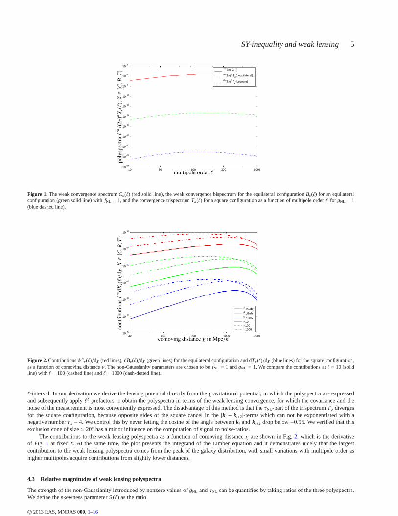
Fig. 1 shows the weak lensing spectrum and the non-Gaussian bi- andtrispectra as a function of multipole orderℓ. For the bispectrumwe choose an equilateral configuration and for the trispectrum a square one, which are in fact lower bounds on the bi- and trispectrumamplitudes for local non-Gaussianities. The polyspectra are multiplied with factors of (ℓ)2n for making them dimensionless and in that waywe were able to show all spectra in a single plot, providing a better physical interpretation of variance, skewness and kurtosis per logarithmic

c© 2013 RAS, MNRAS000, 1–16

SY-inequality and weak lensing 5

10 30 100 300 100010

−24

10−22

10−20

10−18

10−16

10−14

10−12

10−10

10−8

10−6

10−4

l2/(2π) Cκ(l)

l4/(2π)2 Bκ(l,equilateral)

l6/(2π)3 Tκ(l,square)

PSfrag replacements

multipole order ℓ

po

lysp

ectr

aℓ2

n/(

2π

)nXκ(ℓ

),X∈C,B,T

Figure 1. The weak convergence spectrumCκ(ℓ) (red solid line), the weak convergence bispectrum for the equilateral configurationBκ(ℓ) for an equilateralconfiguration (green solid line) withfNL = 1, and the convergence trispectrumTκ(ℓ) for a square configuration as a function of multipole orderℓ, for gNL = 1(blue dashed line).

30 100 300 1000 300010

−40

10−35

10−30

10−25

10−20

10−15

10−10

l2 dC/dχl4 dB/dχl6 dT/dχl=10l=100l=1000

PSfrag replacements

comoving distance χ in Mpc/h

con

trib

uti

on

sℓ2

nd

Xκ(ℓ

)/dχ

,X∈C,B,T

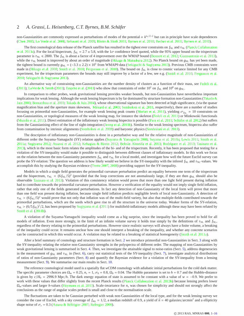
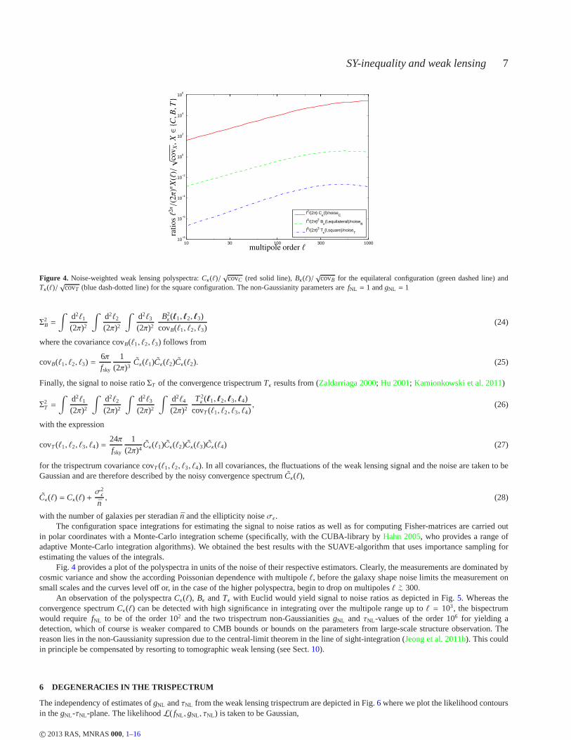
Figure 2. Contributions dCκ(ℓ)/dχ (red lines), dBκ(ℓ)/dχ (green lines) for the equilateral configuration and dTκ(ℓ)/dχ (blue lines) for the square configuration,as a function of comoving distanceχ. The non-Gaussianity parameters are chosen to befNL = 1 andgNL = 1. We compare the contributions atℓ = 10 (solidline) with ℓ = 100 (dashed line) andℓ = 1000 (dash-dotted line).

ℓ-interval. In our derivation we derive the lensing potential directly from the gravitational potential, in which the polyspectra are expressedand subsequently applyℓ2-prefactors to obtain the polyspectra in terms of the weak lensing convergence, for which the covariance and thenoise of the measurement is most conveniently expressed. The disadvantage of this method is that theτNL-part of the trispectrumTψ divergesfor the square configuration, because opposite sides of the square cancel in the|ki − ki+2|-terms which can not be exponentiated with anegative numberns − 4. We control this by never letting the cosine of the angle betweenki and ki+2 drop below−0.95. We verified that thisexclusion cone of size≃ 20 has a minor influence on the computation of signal to noise-ratios.

The contributions to the weak lensing polyspectra as a function of comoving distanceχ are shown in Fig.2, which is the derivativeof Fig. 1 at fixed ℓ. At the same time, the plot presents the integrand of the Limber equation and it demonstrates nicely that the largestcontribution to the weak lensing polyspectra comes from thepeak of the galaxy distribution, with small variations withmultipole order ashigher multipoles acquire contributions from slightly lower distances.

4.3 Relative magnitudes of weak lensing polyspectra

The strength of the non-Gaussianity introduced by nonzero values ofgNL andτNL can be quantified by taking ratios of the three polyspectra.We define the skewness parameterS(ℓ) as the ratio

c© 2013 RAS, MNRAS000, 1–16

6 A. Grassi, L. Heisenberg, C.T. Byrnes, B.M. Schafer

101

102

103

10−16

10−14

10−12

10−10

10−8

10−6

10−4

10−2

kurtosis parameter K(l)skewness parameter S(l)ratio Q(l)

PSfrag replacements

multipole order ℓ

no

n-G

auss

ian

ity

rati

os

K(ℓ

),S

(ℓ),

Q(ℓ

)

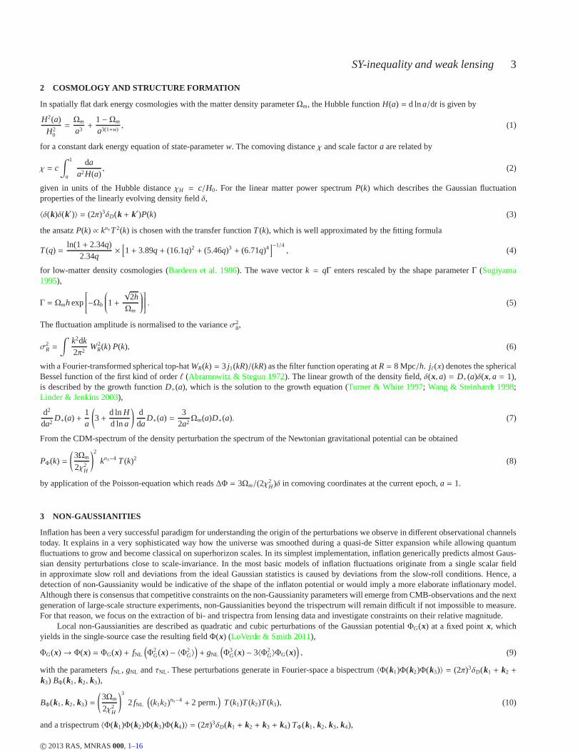
Figure 3. ParametersK(ℓ) (blue solid line),S(ℓ) (green dashed line) andQ(ℓ) (red dash-dotted line), where we chose a equilateral configuration for theconvergence bispectrum and a square configuration for the trispectrum. The non-Gaussianity parameters arefNL = 1 andgNL = 1

S(ℓ) =Bκ(ℓ)

Cκ(ℓ)3/2(19)

between the convergence bispectra for the equilateral configuration and the convergence spectrum. In analogy, we definethe kurtosis param-eterK(ℓ),

K(ℓ) =Tκ(ℓ)Cκ(ℓ)2

, (20)

as the ratio between the convergence trispectrum for the square configuration and the spectrum as a way of quantifying thesize of thenon-Gaussianity. The relative magnitude of the bi- and trispectrum is given by the functionQ(ℓ),

Q(ℓ) =Tκ(ℓ)

Bκ(ℓ)4/3. (21)

For computing the three parameters we set the non-Gaussianity parameters tofNL = gNL = 1.The parameters are shown in Fig.3 as a function of multipole orderℓ. They have been constructed such that the transfer functionT(k) in

each of the polyspectra is cancelled. The parameters are power-laws because the inflationary part of the spectrumkns−4 is scale-free and theWick theorem reduces the polyspectra to products of that inflationary spectrum. The amplitude of the parameters reflectsthe proportionalityof the polyspectra to 3Ωm/(2χ2

H) and the normalisation of each mode proportional toσ8. A noticeable outcome in the plot is the fact that theratio is largest on large scales as anticipated, because thefluctuations in the inflationary fields give rise to fluctuations in the gravitationalpotential on which the perturbation theory is built. Since the effect of the potential is on large scale and the trispectrum is proportional to thespectrum taken to the third power, the ratioK(ℓ) should be the largest on large scales. Therefore as one can see in the Fig.3 the ratio dropsto very small numbers on small scales. Similar arguments apply to Q(ℓ) andS(ℓ), although the dependences are weaker.

5 SIGNAL TO NOISE-RATIOS

The signal strength at which a given polyspectrum can be measured is computed as the ratio between that particular polyspectrum and thevariance of its estimator averaged over a Gaussian ensemble(which, in the case of structure formation non-Gaussianities, has been shownto be a serious limitationTakada & Jain 2009; Sato & Nishimichi 2013; Kayo et al. 2013). We work in the flat-sky approximation becausethe treatment of the bi- and trispectra involves a configuration-space average, which requires the evaluation of Wigner-symbols in multipolespace.

In the flat-sky approximation the signal to noise ratioΣC of the weak convergence spectrumCκ(ℓ) reads (Tegmark et al. 1997; Cooray& Hu 2001)

Σ2C =

∫

d2ℓ

(2π)2

Cκ(ℓ)2

covC(ℓ), (22)

with the Gaussian expression for the covariance covC(ℓ) (Hu & White 2001; Takada & Hu 2013),

covC(ℓ) =2

fsky

12π

Cκ(ℓ)2. (23)

Likewise, the signal to noise ratioΣB of the bispectrumBκ(ℓ) is given by (Hu 2000; Takada & Jain 2004; Babich 2005; Joachimi et al. 2009)

c© 2013 RAS, MNRAS000, 1–16

SY-inequality and weak lensing 7

10 30 100 300 100010

−8

10−6

10−4

10−2

100

102

104

106

l2/(2π) Cκ(l)/noiseC

l4/(2π)2 Bκ(l,equilateral)/noiseB

l6/(2π)3 Tκ(l,square)/noiseT

PSfrag replacements

multipole order ℓ

rati

osℓ2

n/(

2π

)nX

(ℓ)/√

cov

X,

X∈C,B,T

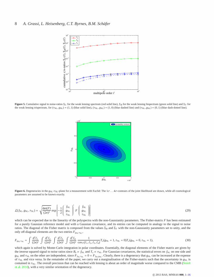
Figure 4. Noise-weighted weak lensing polyspectra:Cκ(ℓ)/√

covC (red solid line),Bκ(ℓ)/√

covB for the equilateral configuration (green dashed line) andTκ(ℓ)/

√covT (blue dash-dotted line) for the square configuration. The non-Gaussianity parameters arefNL = 1 andgNL = 1

Σ2B =

∫

d2ℓ1

(2π)2

∫

d2ℓ2

(2π)2

∫

d2ℓ3

(2π)2

B2κ(ℓ1, ℓ2, ℓ3)

covB(ℓ1, ℓ2, ℓ3)(24)

where the covariance covB(ℓ1, ℓ2, ℓ3) follows from

covB(ℓ1, ℓ2, ℓ3) =6πfsky

1(2π)3

Cκ(ℓ1)Cκ(ℓ2)Cκ(ℓ2). (25)

Finally, the signal to noise ratioΣT of the convergence trispectrumTκ results from (Zaldarriaga 2000; Hu 2001; Kamionkowski et al. 2011)

Σ2T =

∫

d2ℓ1

(2π)2

∫

d2ℓ2

(2π)2

∫

d2ℓ3

(2π)2

∫

d2ℓ4

(2π)2

T2κ (ℓ1, ℓ2, ℓ3, ℓ4)

covT (ℓ1, ℓ2, ℓ3, ℓ4), (26)

with the expression

covT(ℓ1, ℓ2, ℓ3, ℓ4) =24πfsky

1(2π)4

Cκ(ℓ1)Cκ(ℓ2)Cκ(ℓ3)Cκ(ℓ4) (27)

for the trispectrum covariance covT (ℓ1, ℓ2, ℓ3, ℓ4). In all covariances, the fluctuations of the weak lensing signal and the noise are taken to beGaussian and are therefore described by the noisy convergence spectrumCκ(ℓ),

Cκ(ℓ) = Cκ(ℓ) +σ2ǫ

n, (28)

with the number of galaxies per steradian ¯n and the ellipticity noiseσǫ .The configuration space integrations for estimating the signal to noise ratios as well as for computing Fisher-matricesare carried out

in polar coordinates with a Monte-Carlo integration scheme(specifically, with the CUBA-library byHahn 2005, who provides a range ofadaptive Monte-Carlo integration algorithms). We obtained the best results with the SUAVE-algorithm that uses importance sampling forestimating the values of the integrals.

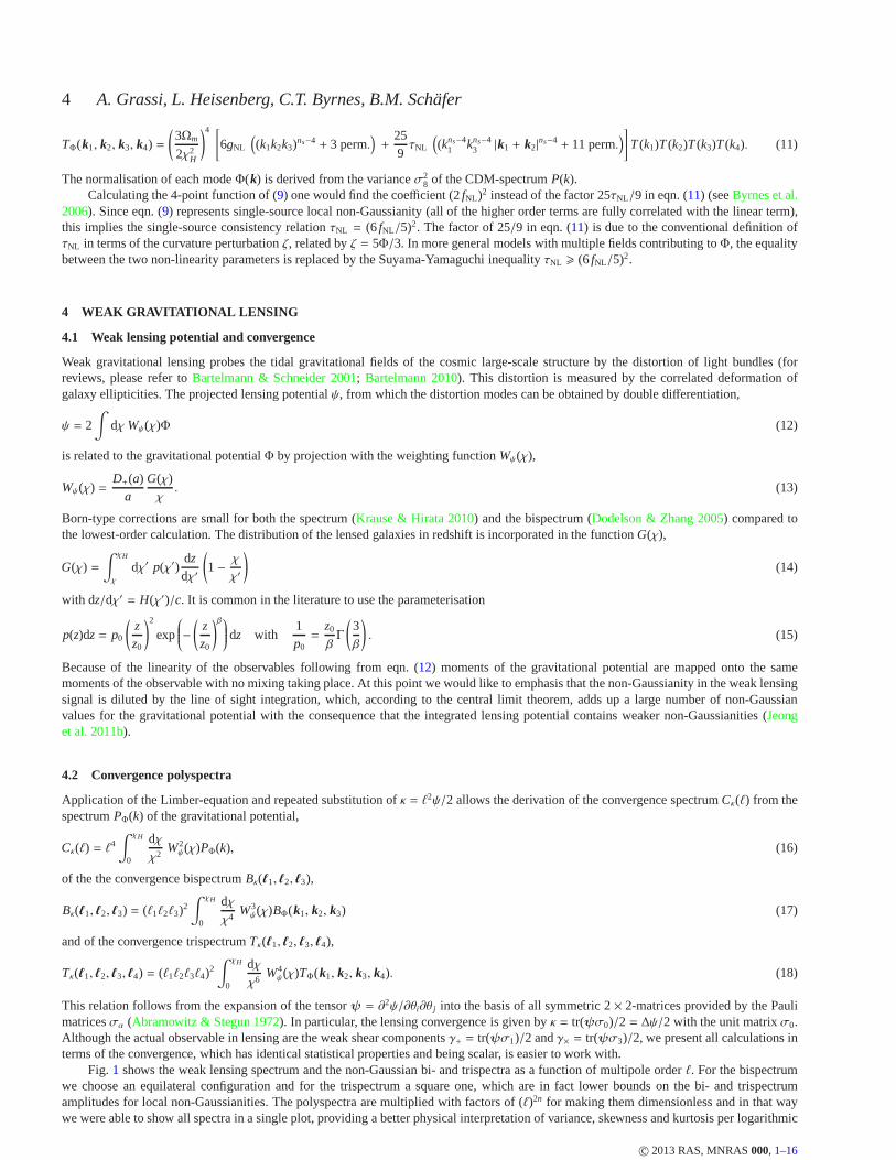
Fig. 4 provides a plot of the polyspectra in units of the noise of their respective estimators. Clearly, the measurements are dominated bycosmic variance and show the according Poissonian dependence with multipoleℓ, before the galaxy shape noise limits the measurement onsmall scales and the curves level off or, in the case of the higher polyspectra, begin to drop on multipolesℓ >∼ 300.

An observation of the polyspectraCκ(ℓ), Bκ andTκ with Euclid would yield signal to noise ratios as depicted inFig. 5. Whereas theconvergence spectrumCκ(ℓ) can be detected with high significance in integrating over the multipole range up toℓ = 103, the bispectrumwould require fNL to be of the order 102 and the two trispectrum non-GaussianitiesgNL and τNL-values of the order 106 for yielding adetection, which of course is weaker compared to CMB bounds or bounds on the parameters from large-scale structure observation. Thereason lies in the non-Gaussianity supression due to the central-limit theorem in the line of sight-integration (Jeong et al. 2011b). This couldin principle be compensated by resorting to tomographic weak lensing (see Sect.10).

6 DEGENERACIES IN THE TRISPECTRUM

The independency of estimates ofgNL andτNL from the weak lensing trispectrum are depicted in Fig.6 where we plot the likelihood contoursin thegNL-τNL-plane. The likelihoodL( fNL ,gNL , τNL) is taken to be Gaussian,

c© 2013 RAS, MNRAS000, 1–16

8 A. Grassi, L. Heisenberg, C.T. Byrnes, B.M. Schafer

101

102

103

10−10

10−8

10−6

10−4

10−2

100

102

104

Σ

C

ΣB

ΣT

PSfrag replacements

multipole order ℓ

cum

ula

tive

s/n

-rat

iosΣ

C(ℓ

),Σ

B(ℓ

),Σ

T(ℓ

)

Figure 5. Cumulative signal to noise-ratiosΣC for the weak lensing spectrum (red solid line),ΣB for the weak lensing bispectrum (green solid line) andΣT forthe weak lensing trispectrum, for (τNL , gNL) = (1, 1) (blue solid line), (τNL , gNL ) = (1, 0) (blue dashed line) and (τNL , gNL ) = (0, 1) (blue dash-dotted line).

−1 −0.5 0 0.5 1

x 107

−1

−0.5

0

0.5

1x 10

7

probability contours

PSfrag replacements

gNL

τN

L

Figure 6. Degeneracies in thegNL -τNL -plane for a measurement with Euclid: The 1σ . . . 4σ-contours of the joint likelihood are drawn, while all cosmologicalparameters are assumed to be known exactly.

L( fNL ,gNL , τNL) =

√

det(F)(2π)3

exp

−12

fNL

gNL

τNL

t

F

fNL

gNL

τNL

(29)

which can be expected due to the linearity of the polyspectrawith the non-Gaussianity parameters. The Fisher-matrixF has been estimatedfor a purely Gaussian reference model and with a Gaussian covariance, and its entries can be computed in analogy to the signal to noiseratios. The diagonal of the Fisher matrix is composed from the valuesΣB andΣT with the non-Gaussianity parameters set to unity, and theonly off-diagonal elements are the two entriesFgNLτNL ,

FgNL τNL =

∫

d2ℓ1

(2π)2

∫

d2ℓ2

(2π)2

∫

d2ℓ3

(2π)2

∫

d2ℓ4

(2π)2

1covT (ℓ1, ℓ2, ℓ3, ℓ4)

Tκ(gNL = 1, τNL = 0)Tκ(gNL = 0, τNL = 1), (30)

which again is solved by Monte-Carlo integration in polar coordinates. Essentially, the diagonal elements of the Fisher matrix are given bythe inverse squared signal to noise ratios sinceBκ ∝ fNL andTκ ∝ τNL . For Gaussian covariances, the statistical errors onfNL on one side andgNL andτNL on the other are independent, sinceF fNL τNL = 0 = F fNL gNL . Clearly, there is a degeneracy thatgNL can be increased at the expenseof τNL and vice versa. In the remainder of the paper, we carry out a marginalisation of the Fisher-matrix such that the uncertainty in gNL iscontained inτNL . The overall precision that can be reached with lensing is about an order of magnitude worse compared to the CMB (Smidtet al. 2010), with a very similar orientation of the degeneracy.

c© 2013 RAS, MNRAS000, 1–16

SY-inequality and weak lensing 9

We compute the Fisher-matrix on the non-Gaussianity parameters with all other cosmological parameter assumed to a level of accuracymuch better than that offNL , gNL andτNL , which is reasonable given the high precision one can reach with in particular tomographic weaklensing spectra, baryon acoustic oscillations and the cosmic microwave background. Typical uncertainties are at least two orders of magnitudebetter than the constraints on non-Gaussianity from weak lensing.

7 TESTING THE SUYAMA-YAMAGUCHI-INEQUALITY

Given the fact that there are a vast array of different inflationary models generating local-type non-Gaussianity, it is indispensable to havea classification of these different models into some categories. This can be for instance achieved by using consistency relations among thenon-Gaussianity parameters as the SY-relation. In the literature one distinguishes between three main categories of models, the single-sourcemodel, the multi-source model and constrained multi-source model. As the name already reveals the single-source modelis a model of onefield causing the non-linearities. The important representatives of this category include the pure curvaton and the pure modulated reheatingscenarios. It is also possible that multiple sources are simultaneously responsible for the origin of density fluctuations. It could be forinstance that both the inflaton and the curvaton fields are generating the non-linearities we observe today. In the case ofmulti-source modelsthe relations between the non-linearity parameters are different from those for the single-source models. Finally, theconstrained multi-sourcemodels are models in which the loop contributions in the expressions for the power spectrum and non-linearity parameters are not neglected.The classification into these three categories was based on the relation betweenfNL andτNL (Suyama et al. 2010b). Nevertheless, this will notbe enough to discriminate between the models of each category. For this purpose, we will need further relations betweenfNL andgNL . Hereby,the models are distinguished by rather ifgNL is proportional tofNL ( fNL ∼ gNL) or enhanced or suppressed compared tofNL . Summarizing,the fNL-τNL and fNL-gNL relations will be powerful tools to discriminate models well. In this work we are focusing on the SY-relation betweenfNL andτNL . The Bayesian evidence (for reviews, seeTrotta 2007, 2008) for the SY-relationτNL > (6 fNL/5)2 can be expressed as the fractionα of the likelihoodL that provides support:

α =

∫

τNL>(6 fNL/5)2

dτ′NL

∫

d f ′NL L(

fNL − f ′NL , τNL − τ′NL

)

. (31)

Henceα answers the question as to how likely one would believe in theSY-inequality with inferredf ′NL andτ′NL-values if the true values aregiven by fNL andτNL . Technically,α corresponds to the integral over the likelihood in thefNL-τNL-plane over the allowed region. Ifα = 1,we would fully believe in the SY-inequality, ifα = 0 we would think that the SY-relation is violated. Correspondingly, 1− α would providea quantification of the violation of the SY-relation,

1− α =∫

τNL<(6 fNL/5)2

dτ′NL

∫

d f ′NL L(

fNL − f ′NL , τNL − τ′NL

)

. (32)

We can formulate the integration over the allowed region as well as an integration over the fullfNL-τNL-range of the likelihood multipliedwith the Heaviside-function,

α =

∫

dτ′NL

∫

d f ′NL L( fNL − f ′NL , τNL − τ′NL)Θ(τNL − (6/5 fNL)2). (33)

This function would play the role of a theoretical prior in the fNL-τNL-plane. In this interpretation,α corresponds to the Bayesian evidence,that means the degree of belief that the SY-inequality is correct.

We can test the SY-inequalityτNL > (6 fNL/5)2 up to the errors onfNL andτNL provided by the lensing measurement: Fig.7 showsthe test statisticα( fNL ,gNL , τNL) in the fNL-τNL-plane, where the likelihood has been marginalised over theparametergNL . The blue regimefNL

>∼ 102 is the parameter space which would not fulfill the SY-inequality, whereas the green areaτNL>∼ 105 is the parameter space where

the SY-relation would be fulfilled. Values offNL<∼ 102 andτNL

<∼ 105 are inconclusive and even though non-Gaussianity parameters may beinferred that would be in violation of the SY-relation, the wide likelihood would not allow to derive a statement. Another nice feature is thefact that for largefNL andτNL the relation can be probed to larger precision and the contours are more closely spaced.

In models where the field which generates non-Gaussianity has a quadratic potential, the non-Gaussianity is mainly captured by fNL ,while gNL is negligible. An example is the curvaton scenario, it is only through self-interactions of the curvaton thatgNL may become largeEnqvist et al.(2010).

8 ANALYTICAL DISTRIBUTIONS

In this section we derive the analytical expression for the probability density that the SY-relation is exactly fulfilled, τNL = (6 fNL/5)2, i.e. forthe case (6fNL/5)2/τNL ≡ 1. For this purpose we explore the properties of the distribution

p(Q)dQ with Q =(6 fNL/5)2

τNL(34)

where the parametersfNL andτNL are both Gaussian distributed with meansfNL , τNL and widthsσ fNL andστNL .We will split the derivation into two parts. First of all we will derive the distribution for the productf 2

NL . For this purpose we use thetransformation of the probability density:

c© 2013 RAS, MNRAS000, 1–16

10 A. Grassi, L. Heisenberg, C.T. Byrnes, B.M. Schafer

101 102 103 104

bispectrum amplitude fNL

103

104

105

106

107

108

trispectrum amplitude τNL

0 .0

0 .1

0 .2

0 .3

0 .4

0 .5

0 .6

0 .7

0 .8

0 .9

1 .0

Figure 7. Bayesian evidenceα( fNL , τNL ) in the fNL -τNL -plane. Blue regions correspond to low, green regions to high degrees of belief. The SY-relationτNL = (6 fNL/6)2 is indicated by the red dashed line.

py(y)dy = px(x)dx (35)

with the Jacobian dx/dy = 1/(2√

y) and wherex = fNL andy = x2. Thus we can write the above equality as

py(y) =px(√

y)

2√

y(36)

where the probability distributionpx(x) is given by

px(√

y) =1

√

2πσ2fNL

exp

−(√

y− fNL)2

2σ2fNL

. (37)

Naively written in this way, we would lose half of the distribution and do not obtain the right normalization. Therefore we have to distinguishbetween the different signs ofy. The distribution of a square of a Gaussian distributed variate fNL with mean fNL and varianceσ fNL is givenby

py(y) =1

√

2πσ2fNL

12√

y×

exp

(

− (√

y− fNL )2

2σ2fNL

)

, positive branch of√

y

exp

(

− (−√−y− fNL )2

2σ2fNL

)

, negative branch of√

y(38)

with y = f 2NL . In the special case of normally distributed variates, the above expression would reduce to

py(y) =1

πσ fNLστNL

K0

(

|y|σ fNLστNL

)

(39)

whereKn(y) is a modified Bessel function of the second kind (Abramowitz & Stegun 1972).The next step is now to implement the distribution eqn. (38) into a ratio distribution since we are interested in the distribution of

(6 fNL/5)2/τNL incorporating the additional factor. The ratio distribution can be written down using the Mellin transformation (Arfken &Weber 2005):

p(Q) =∫

|α|dα py(αQ, fNL)pz(α, τNL), (40)

with a Gaussian distribution forz= τNL ,

pz(z) =1

√

2πσ2z

exp

(

− (z− z)2

2σ2z

)

. (41)

In the special case of Gaussian distributed variates with zero mean the distribution would be simply given by the Cauchy distribution(Marsaglia 1965, 2006), but in the general case eqn. (38) needs to be evaluated analytically.

In Fig. 8 we are illustrating the ratio distribution as a function offNL andτNL for Q = 1, i.e. for the case where the SY-relation becomesan equality. The values forfNL run from 1 to 103 andτNL runs from 1 to 106. The variancesσ fNL andστNL are taken from the output of theFisher matrix and correspond toσ fNL = 93 andστNL = 7.5 × 105. We would like to point out the nice outcome, that the distribution hasa clearly visible bumped line along the the SY-equality. Similarly, Fig. 9 shows a number of example distributionsp(Q)dQ for a choice ofnon-Gaussianity parametersfNL andτNL . We letQ run from 1 to 5 and fix the valuesfNL = 102, 103 andτNL = 104, 105, 106.

c© 2013 RAS, MNRAS000, 1–16

SY-inequality and weak lensing 11

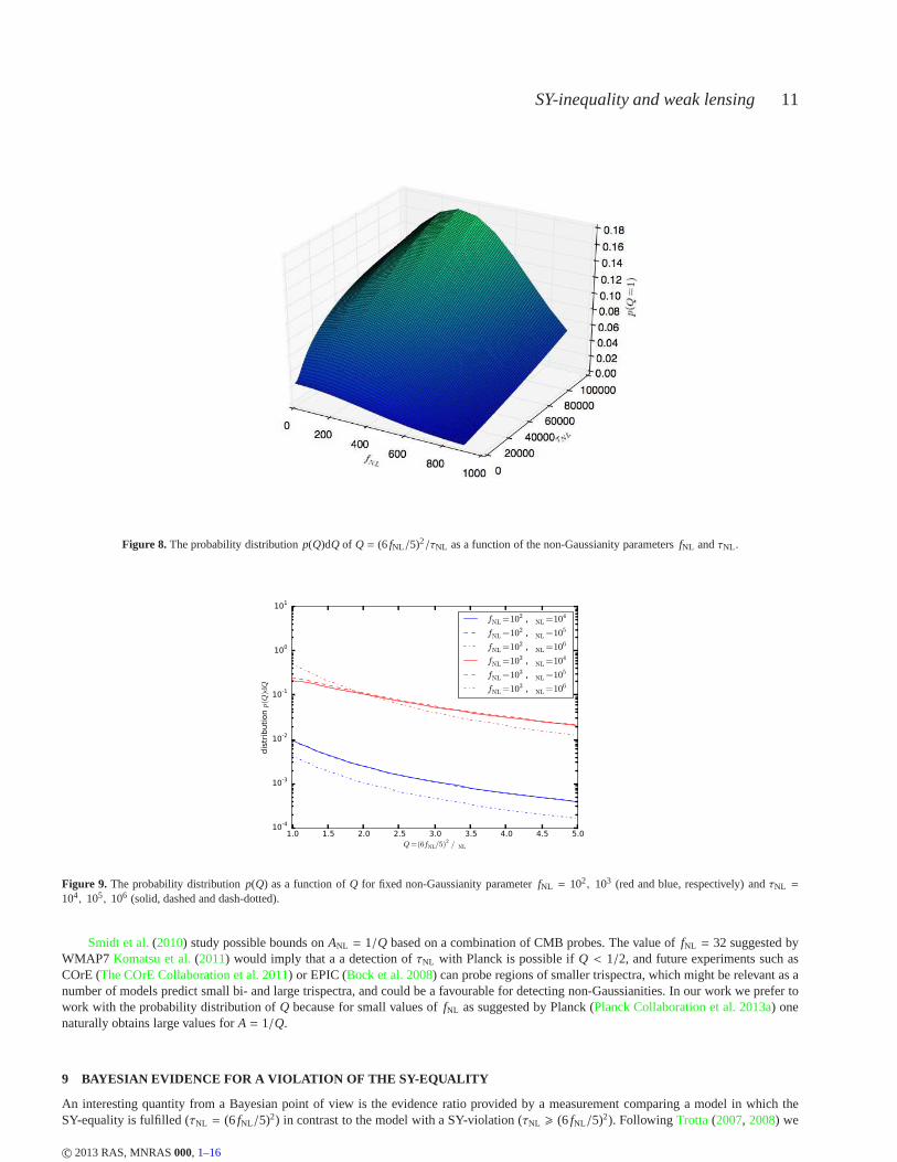
Figure 8. The probability distributionp(Q)dQ of Q = (6 fNL/5)2/τNL as a function of the non-Gaussianity parametersfNL andτNL .

1.0 1.5 2.0 2.5 3.0 3.5 4.0 4.5 5.0Q=(6fNL/5)

2 /τNL

10-4

10-3

10-2

10-1

100

101

distribution p(Q

)dQ

fNL=102 , τNL=104

fNL=102 , τNL=105

fNL=102 , τNL=106

fNL=103 , τNL=104

fNL=103 , τNL=105

fNL=103 , τNL=106

Figure 9. The probability distributionp(Q) as a function ofQ for fixed non-Gaussianity parameterfNL = 102, 103 (red and blue, respectively) andτNL =

104, 105, 106 (solid, dashed and dash-dotted).

Smidt et al.(2010) study possible bounds onANL = 1/Q based on a combination of CMB probes. The value offNL = 32 suggested byWMAP7 Komatsu et al.(2011) would imply that a a detection ofτNL with Planck is possible ifQ < 1/2, and future experiments such asCOrE (The COrE Collaboration et al. 2011) or EPIC (Bock et al. 2008) can probe regions of smaller trispectra, which might be relevant as anumber of models predict small bi- and large trispectra, andcould be a favourable for detecting non-Gaussianities. In our work we prefer towork with the probability distribution ofQ because for small values offNL as suggested by Planck (Planck Collaboration et al. 2013a) onenaturally obtains large values forA = 1/Q.

9 BAYESIAN EVIDENCE FOR A VIOLATION OF THE SY-EQUALITY

An interesting quantity from a Bayesian point of view is the evidence ratio provided by a measurement comparing a model inwhich theSY-equality is fulfilled (τNL = (6 fNL/5)2) in contrast to the model with a SY-violation (τNL > (6 fNL/5)2). FollowingTrotta(2007, 2008) we

c© 2013 RAS, MNRAS000, 1–16

12 A. Grassi, L. Heisenberg, C.T. Byrnes, B.M. Schafer

101 102 103 104

bispectrum amplitude fNL

103

104

105

106

107

108

trispectrum amplitude τNL

− 3 2 0

− 2 8 0

− 2 4 0

− 2 0 0

− 1 6 0

− 1 2 0

− 8 0

− 4 0

0

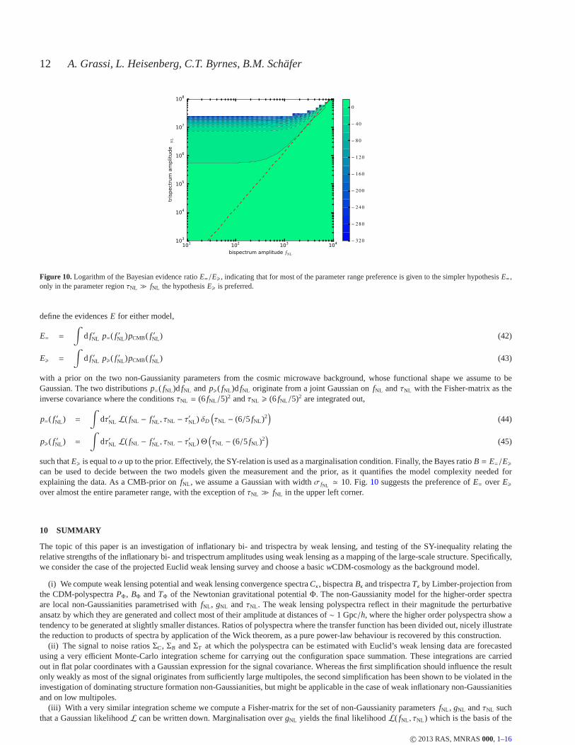
Figure 10. Logarithm of the Bayesian evidence ratioE=/E>, indicating that for most of the parameter range preferenceis given to the simpler hypothesisE=,only in the parameter regionτNL ≫ fNL the hypothesisE> is preferred.

define the evidencesE for either model,

E= =

∫

d f ′NL p=( f ′NL)pCMB( f ′NL) (42)

E> =

∫

d f ′NL p>( f ′NL)pCMB( f ′NL) (43)

with a prior on the two non-Gaussianity parameters from the cosmic microwave background, whose functional shape we assume to beGaussian. The two distributionsp=( fNL)d fNL and p>( fNL)d fNL originate from a joint Gaussian onfNL andτNL with the Fisher-matrix as theinverse covariance where the conditionsτNL = (6 fNL/5)2 andτNL > (6 fNL/5)2 are integrated out,

p=( f ′NL) =

∫

dτ′NL L( fNL − f ′NL , τNL − τ′NL) δD

(

τNL − (6/5 fNL)2)

(44)

p>( f ′NL) =

∫

dτ′NL L( fNL − f ′NL , τNL − τ′NL)Θ(

τNL − (6/5 fNL)2)

(45)

such thatE> is equal toα up to the prior. Effectively, the SY-relation is used as a marginalisation condition. Finally, the Bayes ratioB = E=/E>can be used to decide between the two models given the measurement and the prior, as it quantifies the model complexity needed forexplaining the data. As a CMB-prior onfNL , we assume a Gaussian with widthσ fNL ≃ 10. Fig.10 suggests the preference ofE= over E>over almost the entire parameter range, with the exception of τNL ≫ fNL in the upper left corner.

10 SUMMARY

The topic of this paper is an investigation of inflationary bi- and trispectra by weak lensing, and testing of the SY-inequality relating therelative strengths of the inflationary bi- and trispectrum amplitudes using weak lensing as a mapping of the large-scalestructure. Specifically,we consider the case of the projected Euclid weak lensing survey and choose a basicwCDM-cosmology as the background model.

(i) We compute weak lensing potential and weak lensing convergence spectraCκ, bispectraBκ and trispectraTκ by Limber-projection fromthe CDM-polyspectraPΦ, BΦ andTΦ of the Newtonian gravitational potentialΦ. The non-Gaussianity model for the higher-order spectraare local non-Gaussianities parametrised withfNL , gNL andτNL . The weak lensing polyspectra reflect in their magnitude theperturbativeansatz by which they are generated and collect most of their amplitude at distances of∼ 1 Gpc/h, where the higher order polyspectra show atendency to be generated at slightly smaller distances. Ratios of polyspectra where the transfer function has been divided out, nicely illustratethe reduction to products of spectra by application of the Wick theorem, as a pure power-law behaviour is recovered by this construction.

(ii) The signal to noise ratiosΣC, ΣB andΣT at which the polyspectra can be estimated with Euclid’s weaklensing data are forecastedusing a very efficient Monte-Carlo integration scheme for carrying out the configuration space summation. These integrations are carriedout in flat polar coordinates with a Gaussian expression for the signal covariance. Whereas the first simplification should influence the resultonly weakly as most of the signal originates from sufficiently large multipoles, the second simplification has been shown to be violated in theinvestigation of dominating structure formation non-Gaussianities, but might be applicable in the case of weak inflationary non-Gaussianitiesand on low multipoles.

(iii) With a very similar integration scheme we compute a Fisher-matrix for the set of non-Gaussianity parametersfNL , gNL andτNL suchthat a Gaussian likelihoodL can be written down. Marginalisation overgNL yields the final likelihoodL( fNL , τNL) which is the basis of the

c© 2013 RAS, MNRAS000, 1–16

SY-inequality and weak lensing 13

102 103

multipole ℓ

10-8

10-7

10-6

10-5

10-4

10-3

10-2

10-1

s/n-ratios ΣB and Σ

T

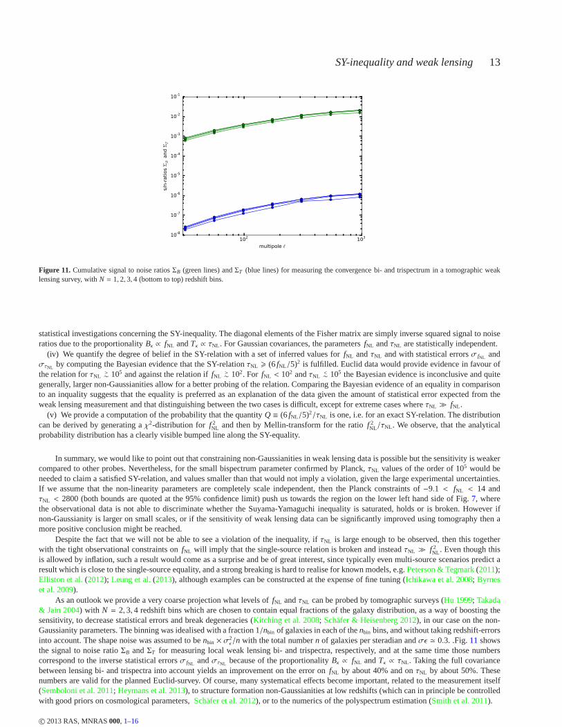
Figure 11. Cumulative signal to noise ratiosΣB (green lines) andΣT (blue lines) for measuring the convergence bi- and trispectrum in a tomographic weaklensing survey, withN = 1, 2, 3, 4 (bottom to top) redshift bins.

statistical investigations concerning the SY-inequality. The diagonal elements of the Fisher matrix are simply inverse squared signal to noiseratios due to the proportionalityBκ ∝ fNL andTκ ∝ τNL . For Gaussian covariances, the parametersfNL andτNL are statistically independent.

(iv) We quantify the degree of belief in the SY-relation witha set of inferred values forfNL andτNL and with statistical errorsσ fNL andστNL by computing the Bayesian evidence that the SY-relationτNL > (6 fNL/5)2 is fulfilled. Euclid data would provide evidence in favour ofthe relation forτNL

>∼ 105 and against the relation iffNL>∼ 102. For fNL < 102 andτNL

<∼ 105 the Bayesian evidence is inconclusive and quitegenerally, larger non-Gaussianities allow for a better probing of the relation. Comparing the Bayesian evidence of an equality in comparisonto an inquality suggests that the equality is preferred as anexplanation of the data given the amount of statistical error expected from theweak lensing measurement and that distinguishing between the two cases is difficult, except for extreme cases whereτNL ≫ fNL .

(v) We provide a computation of the probability that the quantity Q ≡ (6 fNL/5)2/τNL is one, i.e. for an exact SY-relation. The distributioncan be derived by generating aχ2-distribution for f 2

NL and then by Mellin-transform for the ratiof 2NL/τNL . We observe, that the analytical

probability distribution has a clearly visible bumped linealong the SY-equality.

In summary, we would like to point out that constraining non-Gaussianities in weak lensing data is possible but the sensitivity is weakercompared to other probes. Nevertheless, for the small bispectrum parameter confirmed by Planck,τNL values of the order of 105 would beneeded to claim a satisfied SY-relation, and values smaller than that would not imply a violation, given the large experimental uncertainties.If we assume that the non-linearity parameters are completely scale independent, then the Planck constraints of−9.1 < fNL < 14 andτNL < 2800 (both bounds are quoted at the 95% confidence limit) pushus towards the region on the lower left hand side of Fig.7, wherethe observational data is not able to discriminate whether the Suyama-Yamaguchi inequality is saturated, holds or is broken. However ifnon-Gaussianity is larger on small scales, or if the sensitivity of weak lensing data can be significantly improved usingtomography then amore positive conclusion might be reached.

Despite the fact that we will not be able to see a violation of the inequality, ifτNL is large enough to be observed, then this togetherwith the tight observational constraints onfNL will imply that the single-source relation is broken and insteadτNL ≫ f 2

NL . Even though thisis allowed by inflation, such a result would come as a surpriseand be of great interest, since typically even multi-sourcescenarios predict aresult which is close to the single-source equality, and a strong breaking is hard to realise for known models, e.g.Peterson & Tegmark(2011);Elliston et al.(2012); Leung et al.(2013), although examples can be constructed at the expense of finetuning (Ichikawa et al. 2008; Byrneset al. 2009).

As an outlook we provide a very coarse projection what levelsof fNL andτNL can be probed by tomographic surveys (Hu 1999; Takada& Jain 2004) with N = 2,3, 4 redshift bins which are chosen to contain equal fractions of the galaxy distribution, as a way of boosting thesensitivity, to decrease statistical errors and break degeneracies (Kitching et al. 2008; Schafer & Heisenberg 2012), in our case on the non-Gaussianity parameters. The binning was idealised with a fraction 1/nbin of galaxies in each of thenbin bins, and without taking redshift-errorsinto account. The shape noise was assumed to benbin × σ2

ǫ/n with the total numbern of galaxies per steradian andσǫ ≃ 0.3. .Fig.11 showsthe signal to noise ratioΣB andΣT for measuring local weak lensing bi- and trispectra, respectively, and at the same time those numberscorrespond to the inverse statistical errorsσ fNL andστNL because of the proportionalityBκ ∝ fNL andTκ ∝ τNL . Taking the full covariancebetween lensing bi- and trispectra into account yields an improvement on the error onfNL by about 40% and onτNL by about 50%. Thesenumbers are valid for the planned Euclid-survey. Of course,many systematical effects become important, related to the measurement itself(Semboloni et al. 2011; Heymans et al. 2013), to structure formation non-Gaussianities at low redshifts (which can in principle be controlledwith good priors on cosmological parameters,Schafer et al. 2012), or to the numerics of the polyspectrum estimation (Smith et al. 2011).

c© 2013 RAS, MNRAS000, 1–16

14 A. Grassi, L. Heisenberg, C.T. Byrnes, B.M. Schafer

ACKNOWLEDGEMENTS

AG’s and BMS’s work was supported by the German Research Foundation (DFG) within the framework of the excellence initiative throughGSFP+ at Heidelberg and the International Max Planck Research School for astronomy and cosmic physics. LH was supported by theSwissScience Foundation and CTB acknowledges support from the Royal Society. We would like to thank Gero Jurgens for his support concerningthe expressions for the covariance of bi- and trispectra. LHwould like to thank to Claudia de Rham and Raquel Ribeiro for very usefuldiscussions. Finally, we would like to express our gratitude to the anonymous referee for thoughtful questions.

REFERENCES

Abramowitz M., Stegun I. A., 1972, Handbook of MathematicalFunctions. Handbook of Mathematical Functions, New York: Dover, 1972Amara A., Refregier A., 2007, MNRAS, 381, 1018Arfken G. B., Weber H. J., 2005, Materials and ManufacturingProcessesAssassi V., Baumann D., Green D., 2012, JCAP, 1211, 047Babich D., 2005, Phys. Rev. D, 72, 043003Bardeen J. M., Bond J. R., Kaiser N., Szalay A. S., 1986, ApJ, 304, 15Bartelmann M., 2010, Classical and Quantum Gravity, 27, 233001Bartelmann M., Schneider P., 2001, Physics Reports, 340, 291Bartolo N., Komatsu E., Matarrese S., Riotto A., 2004, Physics Reports, 402, 103Becker A., Huterer D., Kadota K., 2011, JCAP, 1101, 006Beltran Almeida J. P., Rodrıguez Y., Valenzuela-Toledo C. A., 2013, Modern Physics Letters A, 28, 50012Bennett C. L., Larson D., Weiland J. L., Jarosik N., Hinshaw G., Odegard N., Smith K. M., Hill R. S., et al. 2012, ArXiv e-prints 1212.5225Bernardeau F., van Waerbeke L., Mellier Y., 2003, A&A, 397, 405Bock J., Cooray A., Hanany S., Keating B., Lee A., Matsumura T., Milligan M., Ponthieu N., et al. 2008, ArXiv e-prints 0805.4207Byrnes C. T., Choi K.-Y., Hall L. M., 2009, JCAP, 0902, 017Byrnes C. T., Enqvist K., Takahashi T., 2010, JCAP, 1009, 026Byrnes C. T., Gerstenlauer M., Nurmi S., Tasinato G., Wands D., 2010, JCAP, 10, 4Byrnes C. T., Sasaki M., Wands D., 2006, Phys.Rev., D74, 123519Byun J., Bean R., 2013, ArXiv e-prints 1303.3050Chen X., 2005, Phys.Rev., D72, 123518Cooray A., Hu W., 2001, ApJ, 554, 56Desjacques V., Seljak U., 2010a, Classical and Quantum Gravity, 27, 124011Desjacques V., Seljak U., 2010b, Advances in Astronomy, 2010Dodelson S., Zhang P., 2005, Phys. Rev. D, 72, 083001Elliston J., Alabidi L., Huston I., Mulryne D., Tavakol R., 2012, JCAP, 1209, 001Enqvist K., Hotchkiss S., Taanila O., 2011, JCAP, 4, 17Enqvist K., Nurmi S., Taanila O., Takahashi T., 2010, JCAP, 1004, 009Fedeli C., Carbone C., Moscardini L., Cimatti A., 2011, MNRAS, 414, 1545Fedeli C., Pace F., Moscardini L., Grossi M., Dolag K., 2011,ArXiv e-prints 1103.5396Fergusson J., Shellard E., 2009, Phys.Rev., D80, 043510Fergusson J. R., Liguori M., Shellard E. P. S., 2010, Phys. Rev. D, 82, 023502Fergusson J. R., Regan D. M., Shellard E. P. S., 2010, ArXiv e-prints 1012.6039Fergusson J. R., Shellard E. P. S., 2007, Phys. Rev. D, 76, 083523Giannantonio T., Ross A. J., Percival W. J., Crittenden R., Bacher D., et al., 2013, arXiv 1303.1349Hahn T., 2005, Computer Physics Communications, 168, 78Heymans C., Grocutt E., Heavens A., Kilbinger M., Kitching T. D., Simpson F., Benjamin J., Erben T., et al. 2013, ArXiv e-prints 1303.1808Hikage C., Matsubara T., 2012, MNRAS, 425, 2187Hikage C., Matsubara T., Coles P., Liguori M., Hansen F. K., Matarrese S., 2008, MNRAS, 389, 1439Hu W., 1999, ApJL, 522, L21Hu W., 2000, Phys. Rev. D, 62, 043007Hu W., 2001, Phys. Rev. D, 64, 083005Hu W., White M., 2001, ApJ, 554, 67Ichikawa K., Suyama T., Takahashi T., Yamaguchi M., 2008, Phys.Rev., D78, 063545Jeong D., Schmidt F., Sefusatti E., 2011a, ArXiv e-prints 1104.0926Jeong D., Schmidt F., Sefusatti E., 2011b, Phys. Rev. D, 83, 123005Joachimi B., Shi X., Schneider P., 2009, A&A, 508, 1193Kamionkowski M., Smith T. L., Heavens A., 2011, Phys. Rev. D,83, 023007Kayo I., Takada M., Jain B., 2013, MNRAS, 429, 344Kehagias A., Riotto A., 2012, Nucl.Phys., B864, 492Kitching T. D., Taylor A. N., Heavens A. F., 2008, MNRAS, 389,173Komatsu E., 2010, Class.Quant.Grav., 27, 124010

c© 2013 RAS, MNRAS000, 1–16

SY-inequality and weak lensing 15

Komatsu E., Afshordi N., Bartolo N., Baumann D., Bond J., et al., 2009, arXiv 0902.4759Komatsu E., et al., 2011, Astrophys.J.Suppl., 192, 18Krause E., Hirata C. M., 2010, A&A, 523, A28+Lesgourgues J., 2013, ArXiv e-prints 1302.4640Leung G., Tarrant E. R. M., Byrnes C. T., Copeland E. J., 2013,arXiv 1303.4678Lewis A., 2011, JCAP, 1110, 026Linder E. V., Jenkins A., 2003, MNRAS, 346, 573Lo Verde M., Miller A., Shandera S., Verde L., 2008, JCAP, 4, 14LoVerde M., Smith K. M., 2011, JCAP, 8, 3Marian L., Hilbert S., Smith R. E., Schneider P., DesjacquesV., 2011, ApJL, 728, L13+Marsaglia G., 1965, Journal of the American Statistical Association, 60, 193Marsaglia G., 2006, Journal of Statistical Software, 16, 1Martin J., Ringeval C., Vennin V., 2013, ArXiv e-prints 1303.3787Menard B., Bartelmann M., Mellier Y., 2003, A&A, 409, 411Munshi D., van Waerbeke L., Smidt J., Coles P., 2011, ArXiv e-prints 1103.1876 1103.1876Pace F., Moscardini L., Bartelmann M., Branchini E., Dolag K., Grossi M., Matarrese S., 2011, MNRAS, 411, 595Peterson C. M., Tegmark M., 2011, Phys.Rev., D84, 023520Pettinari G. W., Fidler C., Crittenden R., Koyama K., Wands D., 2013, JCAP, 4, 3Planck Collaboration Ade P. A. R., Aghanim N., Armitage-Caplan C., Arnaud M., Ashdown M., Atrio-Barandela F., Aumont J., BaccigalupiC., Banday A. J., et al. 2013b, ArXiv e-prints 1303.5076

Planck Collaboration Ade P. A. R., Aghanim N., Armitage-Caplan C., Arnaud M., Ashdown M., Atrio-Barandela F., Aumont J., BaccigalupiC., Banday A. J., et al. 2013a, ArXiv e-prints 1303.5082

Refregier A., 2009, Experimental Astronomy, 23, 17Riotto A., Sloth M. S., 2011, Phys.Rev., D83, 041301Rodrıguez Y., Beltran Almeida J. P., Valenzuela-Toledo C. A., 2013, JCAP, 4, 39Sato M., Nishimichi T., 2013, ArXiv e-prints 1301.3588Schafer B. M., Grassi A., Gerstenlauer M., Byrnes C. T., 2012, MNRAS, 421, 797Schafer B. M., Heisenberg L., 2012, MNRAS, 423, 3445Seery D., Lidsey J. E., Sloth M. S., 2007, JCAP, 1, 27Sefusatti E., Liguori M., Yadav A. P., Jackson M. G., Pajer E., 2009, JCAP, 0912, 022Sekiguchi T., Sugiyama N., 2013, ArXiv e-prints 1303.4626Semboloni E., Heymans C., van Waerbeke L., Schneider P., 2008, MNRAS, 388, 991Semboloni E., Hoekstra H., Schaye J., van Daalen M. P., McCarthy I. G., 2011, ArXiv e-prints 1105.1075Semboloni E., Schrabback T., van Waerbeke L., Vafaei S., Hartlap J., Hilbert S., 2011, MNRAS, 410, 143Smidt J., Amblard A., Byrnes C. T., Cooray A., Heavens A., Munshi D., 2010, Phys. Rev. D, 81, 123007Smidt J., Amblard A., Cooray A., Heavens A., Munshi D., SerraP., 2010, ArXiv e-printsSmith K. M., Loverde M., Zaldarriaga M., 2011a, Physical Review Letters, 107, 191301Smith K. M., Loverde M., Zaldarriaga M., 2011b, Physical Review Letters, 107, 191301Smith T. L., Kamionkowski M., Wandelt B. D., 2011, ArXiv e-prints 1104.0930Sugiyama N., 1995, ApJS, 100, 281Sugiyama N. S., 2012, JCAP, 5, 32Sugiyama N. S., Komatsu E., Futamase T., 2011, Physical Review Letters, 106, 251301Suyama T., Takahashi T., Yamaguchi M., Yokoyama S., 2010a, JCAP, 12, 30Suyama T., Takahashi T., Yamaguchi M., Yokoyama S., 2010b, JCAP, 12, 30Suyama T., Yamaguchi M., 2008, Phys. Rev. D, 77, 023505Takada M., Hu W., 2013, ArXiv e-prints 1302.6994Takada M., Jain B., 2003, MNRAS, 344, 857Takada M., Jain B., 2004, MNRAS, 348, 897Takada M., Jain B., 2009, MNRAS, 395, 2065Tasinato G., Byrnes C. T., Nurmi S., Wands D., 2013, Phys. Rev. D, 87, 043512Tegmark M., Taylor A. N., Heavens A. F., 1997, ApJ, 480, 22The COrE Collaboration Armitage-Caplan C., Avillez M., Barbosa D., Banday A., Bartolo N., Battye R., Bernard J., et al. 2011, ArXive-prints 1102.2181

Trotta R., 2007, MNRAS, 378, 72Trotta R., 2008, Contemporary Physics, 49, 71Turner M. S., White M., 1997, Phys. Rev. D, 56, 4439Verde L., 2010, Advances in Astronomy, 2010Vielva P., Sanz J. L., 2009, MNRAS, 397, 837Wang L., Steinhardt P. J., 1998, ApJ, 508, 483Wang Y., 2013, ArXiv e-prints 1303.1523Zaldarriaga M., 2000, Phys. Rev. D, 62, 063510

c© 2013 RAS, MNRAS000, 1–16

16 A. Grassi, L. Heisenberg, C.T. Byrnes, B.M. Schafer

This paper has been typeset from a TEX/ LATEX file prepared by the author.

c© 2013 RAS, MNRAS000, 1–16