A Theory of Bank Liquidity Requirements∗

Charles W. Calomiris† Florian Heider‡ Marie Hoerova§

January 2015

Abstract

We develop a theory of bank liquidity (cash reserve) requirements. The modelencompasses three motives for requiring bank cash holdings as part of a prudentialregulatory framework: (1) cash is observable and verifiable, (2) because the riskinessof cash is invariant to bankers’ decisions about whether to invest resources in riskmanagement, greater cash holdings improve incentives to manage risk in the non-cashasset portfolio of risky assets held by the bank, and (3) maintaining cash in advancesaves on liquidation costs. In an autarkic banking equilibrium, cash is held voluntarilyby banks as a commitment device to manage risk properly; increasing cash holdingsin response to adverse news stems depositors’ incentives to withdraw funds early. Ina model with multiple banks and information externalities, deposit insurance may beoptimal, and cash reserve requirements are needed to incentivize prudent behaviorby banks. In a model with multiple banks subject to liquidity shocks, the coalitionof banks will commit to lend each other funds in response to bank-specific needs toaccumulate cash; in that equilibrium, cash requirements will be imposed by the groupto prevent free riding on efficient interbank liquidity assistance.

Keywords: Liquidity regulation, reserve requirements, bank runs, deposit insur-ance, moral hazard, risk management

JEL codes: G21, G28, E58, D82

∗We would like to thank our discussants Martin Hellwig, Jean Helwege, Frederic Malherbe, MikeMariathasan, Konstantin Milbradt, Martin Oehmke, Christine Parlour, Enrico Perotti, Lev Ratnovski, An-jan Thakor and Razvan Vlahu, participants in the NBER Risks of Financial Institutions Conference, aswell as numerous seminar participants. Part of this research was conducted while Charles Calomiris was aVisiting Research Fellow at the International Monetary Fund. The views expressed do not necessarily reflectthose of the European Central Bank, the Eurosystem or the International Monetary Fund.†Columbia University, Graduate School of Business, email: cc374@columbia.edu‡European Central Bank, Financial Research Division, email: florian.heider@ecb.int§European Central Bank, Financial Research Division, email: marie.hoerova@ecb.int

1 Introduction

In response to the global financial crisis of 2007-2009, the Basel Committee has proposed a

new global set of liquidity requirements, the Liquidity Coverage Ratio (LCR) and the Net

Stable Funding Ratio (NFSR), to complement its revised framework of international capital

requirements. The primary and obvious motivation for the new interest in managing banks’

liquidity is concern about liquidity risk: “The objective of the LCR is to promote the short-

term resilience of the liquidity risk profile of banks. It does this by ensuring that banks have

an adequate stock of unencumbered high-quality liquid assets that can be converted easily

and immediately in private markets into cash to meet their liquidity needs for a 30 calendar

day liquidity stress scenario” (Basel Committee on Banking Supervision, 2013). After the

malfunctioning of interbank markets and the heavy reliance of banks on central bank lending

during the crisis, policy makers understandably would like to reduce the likelihood of systemic

crises, fire sales, and the dependence of banks on the lender-of-last-resort.

In this paper, we develop a model of liquidity requirements in which the proper focus

of regulation is on the asset side of the bank’s balance sheet, and in which the liquidity

requirement takes the form of a narrow cash reserve requirement. Rather than the Basel III

approach - which seeks to limit rollover risk - we show that the role of liquidity requirements

should be conceived in a more nuanced way, not just as an insurance policy to deal with

liquidity risk that can arise in a financial crisis, but also as a prudential regulatory tool to

make crises less likely. In our framework, cash requirements limit default risk and encourage

good risk management. We show that the primary benefits derived from cash requirements

(like capital requirements) relate to the special role of cash in incentivizing improvements

in bank risk profiles by encouraging proper risk management. Cash holdings reduce the

probability of a liquidity crisis by making banking systems more resilient from a default risk

perspective.

Our framework also provides a resolution to “Goodhart’s Paradox” of liquidity regulation

(Goodhart 2008, Weidmann 2014). Goodhart argues that because cash requirements force

1

banks to hold cash, they may limit the usefulness of having cash to resolve liquidity problems.

In our model, the incentive benefits of cash holdings and cash reserve requirements enable

markets to function better, and their usefulness does not depend on a bank’s ability to

payout the cash to resolve liquidity risk.

Unlike the Basel III approach to liquidity regulation - in which capital standards regulate

default risk and liquidity standards are conceived as protecting against additional exogenous

liquidity shocks - our approach recognizes that illiquidity in markets is almost always a direct

consequence of severe increases in default risk. For example, during the recent U.S. banking

crisis of 2007-2009, the ratios of the market value of equity to assets fell gradually over a

period of more than two years, implying a gradual increase in counterparty risk. At the time

of the failure of Lehman Brothers in September 2008, the counterparty risks of banks such

as Citibank had risen to a critical level (Calomiris and Herring, 2013). The collapse of short-

term funding in repos, commercial paper, and interbank lending in the fall of 2008 was not

an exogenous shock, but rather reflected that rise in counterparty risk; Lehman’s failure was

the proverbial “match in the tinder box,” just as the 2007 asset-backed commercial paper

collapse had reflected the arrival of adverse news about counterparty risk (Heider, Hoerova

and Holthausen, 2009; Gorton and Metrick, 2012; Covitz, Liang, and Suarez, 2013).

The recent crisis was not new in this respect. The history of banking crises is a history of

endogenous collapses of market liquidity that are caused by asymmetric information about

bank default risk. Because bank liabilities have short duration and mainly take the form of

money market instruments, they respond to even small increases in default risk with severe

credit rationing (Calomiris and Gorton, 1991). Indeed, it is noteworthy that the history of

prudential regulation prior to the 1980s focused on cash ratio requirements, not capital ratio

requirements, as the primary regulatory tool. In that sense, our model points toward the

need to restore cash requirements to their rightful place in the prudential regulatory toolkit.

Another empirical observation that motivates our approach is the importance of risk

management for explaining cross-sectional differences in the extent to which banks suffer

2

losses during financial crises. Ellul and Yerramilli (2013) show that the centrality of the

chief risk officer (CRO) within the bank (as measured by the ratio of CRO compensation

relative to CEO compensation) predicts the extent of bank risk taking ex ante and losses

ex post. Fahlenbrach, Prilmeier and Stulz (2012) similarly show that there is a bank fixed

effect in risk management: banks that had the relatively greatest losses in 2008 tended to

be those that also suffered the most severe losses in 1998.

We construct a simple framework of cash requirements in the context of a model in which

both default and liquidity risk arise. We show that, under the assumptions of a parsimonious

model that allows bankers to choose their balance sheet structure and their risk profile, there

is an optimal amount of observable cash assets that a bank holds.

There are two essential differences between capital on the liability side and cash on the

asset side that drive our results: (1) The value of cash held at the central bank is observable

(verifiable) at all times; the value of capital, in contrast, depends on the value of risky assets.

(2) Cash is a riskless asset and so, when banks hold cash, they commit to removing default

risk from a portion of their portfolio. Because cash is both observable and riskless, and is

available to repay senior claim-holders (depositors) in the event of a bank liquidation, the

commitment to hold cash has important implications for bankers’ incentives toward risk in

the future. That commitment affects the way outsiders – who lack information about bank

assets and bankers’ behavior – view the risk management of the bank, which has immediate

consequences for the bank’s access to funding.

In our model, there is a conflict of interest between the banker/owner and outside investor

with respect to risk management; the banker suffers a private cost from managing risk, and

does not always gain enough as the owner to offset that cost. We demonstrate the relative

importance of cash for mitigating both default and liquidity risks by solving our model under

three alternative policy regimes: (1) autarky, in which each bank chooses both its asset and

liability structure in combination with a decision to manage the risk of high-return assets

(e.g., loans) in an environment without liquidity risk, (2) a deposit insurance system created

3

to address information externalities in risk management, and (3) collective action, where a

group of banks forms a coalition to coinsure against liquidity risk.

Under autarky, regulation of liquidity plays no role because there are no externalities

to motivate regulation. The bank voluntarily chooses the socially and individually optimal

combination of cash holdings and loans, trading off the benefit from committing to “incentive-

compatible” risk management from higher cash holdings against the cost of holding low-

return cash assets.

An important insight from the autarky model is that the ability of outsiders to withdraw

their claims plays an important role in encouraging banks to maintain adequate amounts of

cash, especially when “bad” states of the world necessitate a topping up of cash balances.

Without the discipline of a withdrawal threat, the bank has no incentive to increase cash

holdings in bad states of the world. Instead, it would promise to do so but renege on that

promise after outsiders had deposited their funds with the bank. That is, the bank must be

exposed to potential liquidity risk in order for cash to be able to improve risk management.

We next consider a model of the economic efficiency gains from deposit insurance in the

presence of an information externality among banks (depositors cannot distinguish between

sound and weak banks). We show that deposit insurance is optimal when depositors are

sufficiently risk averse, and the subsidy risky banks receive from safe banks is not too high.

We also show that a cash reserve requirement is an important tool in the presence of deposit

insurance (even though deposit insurance eliminates all liquidity risk in the banking system).

Cash requirements are necessary in the presence of deposit insurance as a means of controlling

default risk.

We then examine a role for cash reserve requirements in a model of a banking system

subject to liquidity shocks. We show that the coalition of banks (which we refer to as the

clearinghouse because bank clearinghouses historically were the form of collective action that

managed liquidity risk) is able to achieve a better outcome than banks can achieve under

autarky because liquidity risk is diversifiable across banks. As before, giving depositors a

4

withdrawal option is necessary to implement the socially optimal amount of cash holdings,

which result in optimal risk management. To prevent free riding on collective protection, the

bank coalition will therefore impose a cash reserve requirement on its members (as discussed,

for example, in Gorton, 1985).

Our framework has several implications for the design of liquidity regulation. Rather than

viewing the regulation as ex post insurance, we view it as providing ex ante incentives to

reduce credit risk, which in turn enables banks to better access markets for low-risk, short-

term debt. Our framework stresses the need to regulate cash holdings, not rollover risk,

and crucially, it requires that cash holdings be continuously observable, which requires that

they be held outside the bank (for example, at the central bank). If instead cash was held

inside banks, holding more liquidity might actually lead to greater risk-taking (see Myers

and Rajan, 1998).1

We also emphasize the need to jointly consider liquidity and capital regulation. The

banks in our model make joint decisions about their asset and liability structure. Because

cash reserve requirements ensure efficient and credible risk management, they also make the

book value of equity reported by the bank a more reliable indicator of the true value of equity.

Thus, an important implication of our model is that the use of cash reserve requirements

makes equity ratio requirements more effective.

Finally, the Basel LCR approach views greater reliance on insured deposits as resulting

in less need for cash assets because there is less withdrawal risk. In sharp contrast, in our

model, insured deposits undermine market discipline; required holdings of cash are therefore

needed to compensate for the absence of market discipline.

Section 2 provides a brief review of the literature. Section 3 describes the model. Section

4 presents the benchmark case in which effort is observable and there is no moral hazard

problem. We then consider the problem with moral hazard and autarky in Section 5. Sections

1The failure of MF Global illustrated how financial firms can “window dress” their accounts on quarterlyreporting dates to appear to hold a large amount of cash assets, but those assets can disappear quickly atthe discretion of management when management chooses to invest them in risky assets. See, for example,“MF Global Masked Debt Risks,” Reuters (November 3, 2011).

5

6 and 7 solve for equilibrium under deposit insurance and under collective action, respectively.

Section 8 concludes. All proofs are in the Appendix.

2 Literature Review

A helpful place to begin any discussion of cash reserve requirements is with the Black-

Scholes-Merton framework (e.g., Merton 1977). In that framework, there are no transaction

or information costs, all information that can be known is known equally to all parties, and

all securities are equally (perfectly) liquid – by which we mean that they can be sold for their

true value, which is common knowledge, without incurring any physical liquidation cost. In

that framework, the only special property of cash is its lack of risk. From the standpoint of

prudential regulation – which seeks to avoid the default risk of banks – greater cash holdings

and greater reliance on equity finance each reduce the default risk of the bank.

When one relaxes the assumptions of the Black-Scholes-Merton framework, however, the

effects of cash and equity on default risk are not the same. For example, in Diamond and

Dybvig (1983) physical costs of liquidation make liquidity risk (the possible need to finance

early consumption) costly, which could motivate the holding of inventories of liquid assets.

In Calomiris and Kahn (1991), depositors receive noisy and independent signals about the

risky portfolio outcome of a bank. By holding reserves, banks insulate themselves against the

liquidity risk of a small number of “misinformed” early withdrawals in states of the world

where the outcome is actually good. Without those reserves, banks offering demandable

debt contracts (which are optimal in the Calomiris-Kahn model) would unnecessarily subject

themselves to physical liquidation costs when they fail to meet depositors’ requests for early

withdrawal.

In many models of banking, equity is an undesirable means of controlling risk because

of the high costs of raising equity. Typically, the optimal contract between the banker and

his or her funding sources is a debt contract, and sometimes a demandable debt contract.

6

Debt contracts economize on the cost of ex post verification (Townsend 1979, Diamond 1984,

Gale and Hellwig 1985, Calomiris and Kahn 1991), reduce the negative signaling of bank

type (Myers and Majluf 1984), allow the trading of the outside claim (Gorton and Pennacchi,

1990) and they can limit the hold-up problem between bankers and their borrowers (Diamond

and Rajan, 2001). In our model equity is assumed to be supplied by the banker, and not by

outsiders because of its prohibitively high cost. The outsiders claim is senior to the banker’s

claim and can therefore be thought of as debt. Importantly, it will be optimal to make the

debt demandable.

Given the high costs of external finance via equity, cash holdings can provide a more cost-

effective means of reducing default risk even in the absence of moral-hazard. Moral-hazard

makes default risk endogenous and creates a conflict of interest between bank insiders and

outside investors. The conflict of interest creates a wedge between physical cash-flows and

those that can be credibly pledged to outside investors (see Holmstrom and Tirole 1997,

1998).

Biais, Heider and Hoerova (2012) show that in the context of derivative trading with

moral-hazard in risk-management, optimal hedging contracts may benefit from the use of

variation margins. As we show in the model below, cash holdings can be an especially useful

means of reducing risk through the effects of cash holdings on the incentives of bankers to

expend effort on risk management, especially in economic downturns. Because cash holdings

limit the extent to which debtholders lose from high-risk strategies and the extent to which

bankers can pursue high-risk strategies, more cash helps to better align managers’ incentives

with the interest of debtholders.

Our paper builds on the insights of these various models. Like Diamond and Dybvig

(1983) we assume that exogenous demand for early liquidation can be physically costly,

which gives rise to liquidity risk in our model. Like Holmstrom and Tirole (1997, 1998), we

assume that risk management entails private costs to the bank manager. In such a context,

cash is doubly important, not just because of its lack of risk, but also because of its ob-

7

servability. Outsiders investors can be confident that managers will exert effort for proper

risk management irrespective of the unobservable state, if and only if cash margins are suf-

ficiently high. As in Biais, Heider and Hoerova (2012), setting aside cash on a separate

account has the benefit of curbing the moral-hazard in risk-management but carries the (op-

portunity) cost of having less invested in a high-return asset. In equilibrium, a withdrawable

senior claim (e.g, deposits) for outsiders and a sufficient amount of cash reserves provide

an optimal contractual solution to the banking problem that combines all those elements:

That solution minimizes the overall costs associated with early liquidation, shirking in risk

management and foregone opportunities for profits (from cash holdings).

The role of cash in our banking environment resembles at first glance the role of collateral

in environments with adverse selection (Besanko and Thakor 1987) or moral hazard (Boot

and Thakor 1994). There are, however, important differences. First, the use of cash can

easily be made contingent on the state of the economic environment. While this in principle

is also possible for traditional collateral, say a banker’s house, it is unlikely to be feasible

in practice. The value of the house will also depend on the economic environment and,

moreover, the value will probably not be enough relative to the size of the incentive problem

of a typical bank. This relates to the second difference. While the amount of collateral is

usually taken as given, the amount of cash is endogenous. It depends on the portfolio choice

of the banker. Moreover, and again related, the value of collateral is usually assumed to be

lower in the hands of lenders than in the hands of borrowers. In contrast, the cost of cash is

an opportunity cost. It arises from not having invested in high-risk/high-return assets such

as loans.

It is also interesting to note the long tradition in banking – despite the absence of formal

modeling – that has focused on cash requirements as a prudential device. Indeed, with few

exceptions, historical prudential regulation prior to the 1980s has concentrated on require-

ments for cash rather than requirements for capital. For example, the New York Clearing

8

House maintained a 25% cash reserve requirement against deposits for its members.2 In the

famous 1873 Coe Report, authored by George Coe, the President of the New York Clearing

House, cash was seen as the essential tool for managing systemic risk (Wicker 2000). In

contrast, neither regulators nor bank coalitions set minimum equity capital-to-asset ratios

for banks, with few exceptions, until the 1980s.3

The observability advantage of cash has been particularly obvious in the recent history

of financial crises in our current highly regulated and protected banking environment, where

government both insures deposits and regulates banks’ risk-based capital requirements. In

this environment, depositors or other banks have little incentive to monitor banks or penalize

high risk. Supervisors, who are charged with protecting taxpayers from the costs of bailing

out banks, typically have not identified bank losses in a timely way. That fact reflects a com-

bination of problems, including the absence of private incentives for supervisors to invest in

monitoring, and the presence of political pressures on supervisors to avoid recognizing losses

(Calomiris and Herring 2013). For example, in December 2008, as an insolvent Citibank

was bailed out by the U.S. government, its ratio of book capital to risk-weighted assets still

exceeded 11%.

In private interbank coalitions, it is easy to see why cash would be especially valued over

equity capital as a tool. Not only does cash mitigate the costs of raising equity ex ante

and mitigate liquidity risks ex post, a greater reliance on observable cash (rather than hard-

to-observe equity) to manage free-riding problems has additional advantages in the context

of a private coalition of competing banks. For bankers to verify each other’s capital in a

precise way they would have to be able to demonstrate the value of each bank’s capital to

the group. Given the private information inherent in bank lending, doing so would require

a significant expenditure of cost. Furthermore, a full analysis of the value of a bank’s loan

2An additional motivation for New York City banks to maintain high required reserves was that city’sposition at the peak of the “reserve pyramid” that connected banks throughout the United States eventhough it generally did not employ its reserves to protect banks in other regions or non-clearing housemembers during financial crises.

3Some of those exceptions were the state experiments with deposit insurance, for example, in the early20th century (see Calomiris, 1990).

9

portfolio would require the sharing of information about loan customers, and such sharing

would destroy quasi rents banks earn from investing in private information (Rajan 1992);

thus, a policy of collective monitoring of each bank’s capital would entail huge information

costs to banks, and erode the incentive for banks to invest in client-specific information. Our

models of collective action developed below do not consider these quasi-rent-erosion costs of

enforcing capital requirements in a banking coalition, but obviously, if they were included,

they would magnify the gains from the use of cash to manage default risk.

3 The Model

There are six dates, t = 0, 1, 2, 3, 4, and 5, and two types of agents, bankers and depositors.

Bankers are risk-neutral. We consider both the case of risk-neutral depositors, as well as the

case of risk-averse depositors.

At time 0, a banker is endowed with knowledge about a prospective loan making oppor-

tunity, and with own equity E0 > 0. A banker accepts deposits D at time 0, which are in

perfectly elastic supply to a banker up to a maximum of D.4 Instead of depositing funds in

a bank, depositors can store their funds, which yields a per-unit return of one for sure.

At time 0, a banker can invest a bank’s resources, D+E0, in cash (the amount invested

in cash is denoted C0) or in loans (the amount invested in loans is denoted L0, which is

also the number of loans since the loan size is normalized to 1). Hence, C0 + L0 = D + E0.

The payoff from the loan will occur at time 5 if the loan is allowed to mature. That payoff

per unit invested will either be Y > 1 or 0. The probability of the high payoff depends on

a banker’s costly risk-management effort at time 4. If he exerts effort, the high payoff Y

occurs for sure and if he does not exert effort, Y occurs only with probability p < 1. The

outcome for each bank that does not exert effort is i.i.d. and by the law of large numbers it is

certain that p proportion of the banks not exerting effort will receive the high payoff. When

4For simplicity, we assume a maximum supply of deposits. This is a reduced form to capture an increasingcost of attracting more deposits due to, e.g., geographical distance. Alternatively, we could assume a limitedamount of loan-making opportunities.

10

a banker chooses not to exert effort, he derives a private benefit B per loan (equivalently,

when not exerting effort, a banker saves on costly risk management). The effort choice of a

banker is unobservable to depositors.

At time 1, a fraction π of depositors experience an exogenous liquidity shock requiring

them to transfer µD cash “abroad” from their deposit account. We set π = 0 for most of

our modeling, but subsequently relax that assumption in Section 7.

At time 2, there are two possible aggregate states s, good or bad, s = {g, b}. The

probability of the good state occurring is denoted by q (the bad state occurs with probability

1 − q). The aggregate state is observed for free by a banker. If depositors want to observe

the aggregate state, they need to spend m (e.g., they invest in a perfectly revealing signal

about the aggregate state). In the bad aggregate state, the private benefit of a banker is

larger, making risk management more costly, than in the good aggregate state, Bg < Bb.

This assumption can be viewed as capturing, in a reduced-form, a set-up with costly loan

monitoring (whereby the frequency of monitoring should be higher in bad times to achieve

the same probability of repayment) or a set-up with searching for prospective loan applicants

and/or screening out bad borrowers (which is more difficult in bad economic times). We let

B denote the expected private benefit of a banker, i.e. B ≡ qBg + (1− q)Bb. We assume

that

Y > 1 > qY + (1− q) (pY +Bb) . (1)

The first inequality implies that when a banker exerts risk-management effort, loan making

has a positive NPV. The second inequality implies that unless a banker does risk-management

effort in both aggregate states, loan making is socially wasteful: even after accounting for

the (maximum) private benefit of a banker, it is more profitable to store funds.5

At t = 3, after learning the aggregate state, a banker can increase his cash holdings

by ∆C (s) by liquidating an amount ∆L (s) of loans. But converting loans into cash at

5The expression on the right-hand side of (1) is the return from exerting effort in the good state and notexerting effort in the bad state. Since Bb > Bg and, by (1), Y > pY + Bb, this is the maximum expectedreturn that can be generated if a banker does not exert effort in at least one aggregate state.

11

t = 3 is costly, ∆C (s) = (1− l) ∆L (s), where l is the cost of liquidation per unit of

loans when loans are liquidated prior to maturity. A banker’s cash holdings at time 3

and state s are C3 (s) = C0 + ∆C (s), while his loan holdings are reduced to L3 (s) =

L0 − ∆L (s) = L0 − ∆C (s) 11−l . Note that the liquidation of loans reduces the value of

equity, E3 = C3 + L3 −D = E0 −∆C (s) l1−l .

The purpose of having liquid assets prior to time 4 is to incentivize the banker to exert

risk-management effort. The banker’s incentive to exert effort, and thus to increase the

probability of high payoff, is lower in the bad aggregate state. By increasing liquid assets at

time 3, the banker will be able to respond to the observed bad aggregate state by increasing

liquid assets, and thereby make risk-management effort at time 4 credible.

At the end of t = 3, depositors choose whether or not to “run” their bank, i.e., whether

or not to shut down the bank. We assume that one depositor’s announcement is enough to

shut down the bank. This can be understood, for example, as an environment in which one

depositor has a low cost m of observing the aggregate state, while the other depositors face

prohibitive costs (so that only one of the depositors is informed). The informed depositor

can be seen as causing the bank to close by withdrawing his or her funds and triggering

imitative withdrawals by other depositors (who, in equilibrium, would not otherwise run the

bank). For simplicity, we adopt a liquidation rule that when a bank is shut down, a banker

surrenders all claims to the bank’s assets. Depositors liquidate the loan portfolio at a cost v

per unit of loans. We assume that depositors face a higher cost of liquidation cost than the

banker, i.e., v > l. Hence, if the bank is shut down, depositors receive the liquidation value

of loans plus the cash in the bank, (1− v)L3 (s) + C3 (s).

At time 4, a banker chooses whether or not to exert risk-management effort. Effort is

not contractible since it is not observable by anyone but the banker himself.

At time 5, the loan outcome Y or 0 is realized. If the high payoff is realized, then

depositors receive R and the banker receives the residual, Y L3 (s) + C3 (s) − R. If the low

payoff is realized, depositors receive Rf ≤ C3 (s). Note that holding cash allows the banker

12

to pay depositors a positive amount even if the loan returns nothing.6

In sum, the timeline is as follows:

Time 0: E0 and D are invested in L0 and C0 and the contract promises (R,Rf ).

Time 1: Exogenous deposit withdrawals of µD occur with probability π.

Time 2: The state is revealed and a banker updates his private benefit Bs based on the

aggregate state. Depositors choose whether or not to spend m to observe the state.

Time 3: A banker can increase cash-holdings by liquidating some loans, where the new

amount of cash is given by C3 (s). Depositors choose whether or not to shut down the bank.

Time 4: A banker decides whether to exert unobservable risk-management effort.

Time 5: A banker pays R if outcome is Y and Rf if outcome is 0.

4 First-best Equilibrium

We now consider the case in which a banker’s risk-management effort is publicly observable

so that there is no moral hazard problem. While implausible, it offers a benchmark against

which we will identify the inefficiencies generated by moral hazard. We solve for the optimum

under the assumption of depositor risk-neutrality, and then show that the equilibrium is the

same under risk aversion.

In the first-best, efficiency requires that a banker does risk-management effort since loan

making is only productive when a banker exerts effort (condition (1)). Moreover, cash is not

used. This is because cash is dominated in terms of rate-of-return compared to loan making

when accompanied by risk-management effort, and there are no incentive benefits of cash

since incentive problems are absent in the first-best. Hence, E0 + D = L0, C0 = C3 (s) = 0

and loans always return Y per unit invested. Note also that depositors do not need to spend

m to observe the aggregate state (to gauge how costly risk-management is for the banker):

6Note that with our two-point distribution, there is no real difference in the cash-flows between debt andequity for the outside claim held by depositors. We can explicitly derive the cash-flows of the outside claim tobe like in a debt contract using costly state verification. Cash would then serve an additional function in themodel, namely economizing on verification costs. For the sake of simplicity, and without loss of generality,we avoid this complication in our model.

13

They can observe their banker’s effort directly and write contracts that guarantee the banker

will exert effort.

Depositors are willing to deposit with a banker as long as the contract offers them at

least the same payoff as storage. That is, the participation constraint of depositors is given

by:

R ≥ D. (2)

Since a banker has a unique ability to make loans, he will not leave depositors any rents,

i.e., R = D. Every deposit brought in earns Y −1 > 0 implying that it is optimal to operate

the bank at the maximum scale. Hence, if a banker chooses to take in deposits, his payoff

at t = 5 is:

Y E0 + (Y − 1)D. (3)

A banker prefers to take in deposits and operate the bank rather than invest solely his

own equity as long as he earns more by operating the bank with deposits compared to

investing his equity only:

Y E0 + (Y − 1)D ≥ Y E0, (4)

which is satisfied since Y > 1. Moreover, it is optimal not to allow depositors to withdraw

early.

Proposition 1 summarizes the first-best outcome.

Proposition 1 When risk-management effort is observable, a banker exerts effort, cash is

never used, and depositors do not spend the cost of observing the aggregate state.

Note that the optimal contract entails a deterministic payoff D for depositors and there-

fore, this is also the optimal contract under depositor risk-aversion.

14

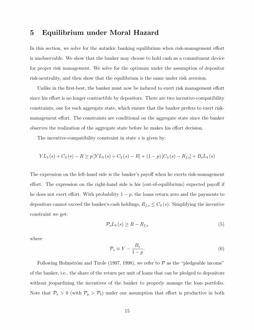
5 Equilibrium under Moral Hazard

In this section, we solve for the autarkic banking equilibrium when risk-management effort

is unobservable. We show that the banker may choose to hold cash as a commitment device

for proper risk management. We solve for the optimum under the assumption of depositor

risk-neutrality, and then show that the equilibrium is the same under risk aversion.

Unlike in the first-best, the banker must now be induced to exert risk management effort

since his effort is no longer contractible by depositors. There are two incentive-compatibility

constraints, one for each aggregate state, which ensure that the banker prefers to exert risk-

management effort. The constraints are conditional on the aggregate state since the banker

observes the realization of the aggregate state before he makes his effort decision.

The incentive-compatibility constraint in state s is given by:

Y L3 (s) + C3 (s)−R ≥ p [Y L3 (s) + C3 (s)−R] + (1− p) [C3 (s)−Rf,s] +BsL3 (s)

The expression on the left-hand side is the banker’s payoff when he exerts risk-management

effort. The expression on the right-hand side is his (out-of-equilibrium) expected payoff if

he does not exert effort. With probability 1− p, the loans return zero and the payments to

depositors cannot exceed the banker’s cash holdings, Rf,s ≤ C3 (s). Simplifying the incentive

constraint we get:

PsL3 (s) ≥ R−Rf,s (5)

where

Ps ≡ Y − Bs

1− p. (6)

Following Holmstrom and Tirole (1997, 1998), we refer to P as the “pledgeable income”

of the banker, i.e., the share of the return per unit of loans that can be pledged to depositors

without jeopardizing the incentives of the banker to properly manage the loan portfolio.

Note that Ps > 0 (with Pg > Pb) under our assumption that effort is productive in both

15

aggregate states (see (1)).

Note that setting the (out-of-equilibrium) payoff to depositors Rf,s as high as possible

relaxes the incentive constraint. Hence, it is optimal to set Rf,s = C3 (s). Moreover, the

participation constraint of depositors is given by (2) and, as before, the banker does not

want to leave any surplus to depositors, so the participation constraint binds, R = D. Using

L3 (s) = L0 −∆C (s) 11−l , C3 (s) = C0 + ∆C (s), and L0 = D +E0 −C0, we can re-write (5)

as

Ps (D + E0) + (1− Ps)C0 +

(1− Ps

1− l

)∆C (s) ≥ D. (7)

Note that 1 − Ps > 1 − Ps

1−l . Moreover, if Ps ≥ 1 in both aggregate states, then cash

holdings cannot help with incentives as they tighten the incentive constraints. Hence, cash

will not be held in this case, implying that the incentive constraints simplify to Ps (D + E0) ≥

D. This is always satisfied for Ps ≥ 1. We can thus state the following lemma.

Lemma 1 When risk-management effort is not observable, but Ps ≥ 1 in both aggregate

states, the first-best is always reached.

Moreover, note that even when Ps < 1, as long as Ps

1−Ps≥ D

E0, the first-best can be reached

with C0 = ∆C (s) = 0. In what follows, we focus on the case in which the first-best is not

attainable, i.e., Ps < 1 and Ps

1−Ps< D

E0in at least one aggregate state. Since Pg > Pb, we

assume that the first-best is not attainable in the bad aggregate state.

5.1 Aggregate State Observable at No Cost

Here we demonstrate that the optimal second-best contract under the assumptions above

has the following key attributes: the bank offers the depositor a senior claim D on the bank

(when the bank is insolvent, the depositor receives the whole value of the bank, which is

less than D), and gives the depositor an option to close down (run) the bank after the

non-contractible state is revealed.7 By offering this contract to the depositor, the banker

7Outside funding is given a senior claim in equilibrium. Thus equity is limited to inside equity in ourmodel, and banks operate at a corner solution, utilizing all inside equity in the bank. It would be possible

16

ensures that he will generate sufficient amounts of cash in the bad state so as to incentivize

himself to undertake the privately costly risk-management effort. In equilibrium, there are

no depositor runs because the banker always creates sufficient reserves in the bad state, and

there is no bank insolvency because the bank’s investments always generate Y when the

banker invests in risk management.

The social cost of this arrangement is the opportunity cost of generating cash, which is

the amount of foregone lending opportunities and the physical liquidation cost that results

from transforming loans into cash reserves. We first show that the contract described here

is feasible. We then consider, in Section 5.2, whether there is an alternative contract based

on banker communication via cash reserve accumulation (a form of “messaging”) that would

be less wasteful because it would economize on cash in the bad state. A contract that would

credibly lower promised payments to depositors in the bad state would reduce the amount

of cash reserves that need to be accumulated. We show that such a contract is not feasible,

which implies that the second-best contract pays a fixed deposit amount D and needs to be

enforced by the threat of a depositor run.

We start by characterizing the case in which depositors can observe the aggregate state

at zero cost, m = 0. We consider the case in which m > 0, and the depositor’s choice of

whether or not to expend m and observe the state, in Section 5.3.

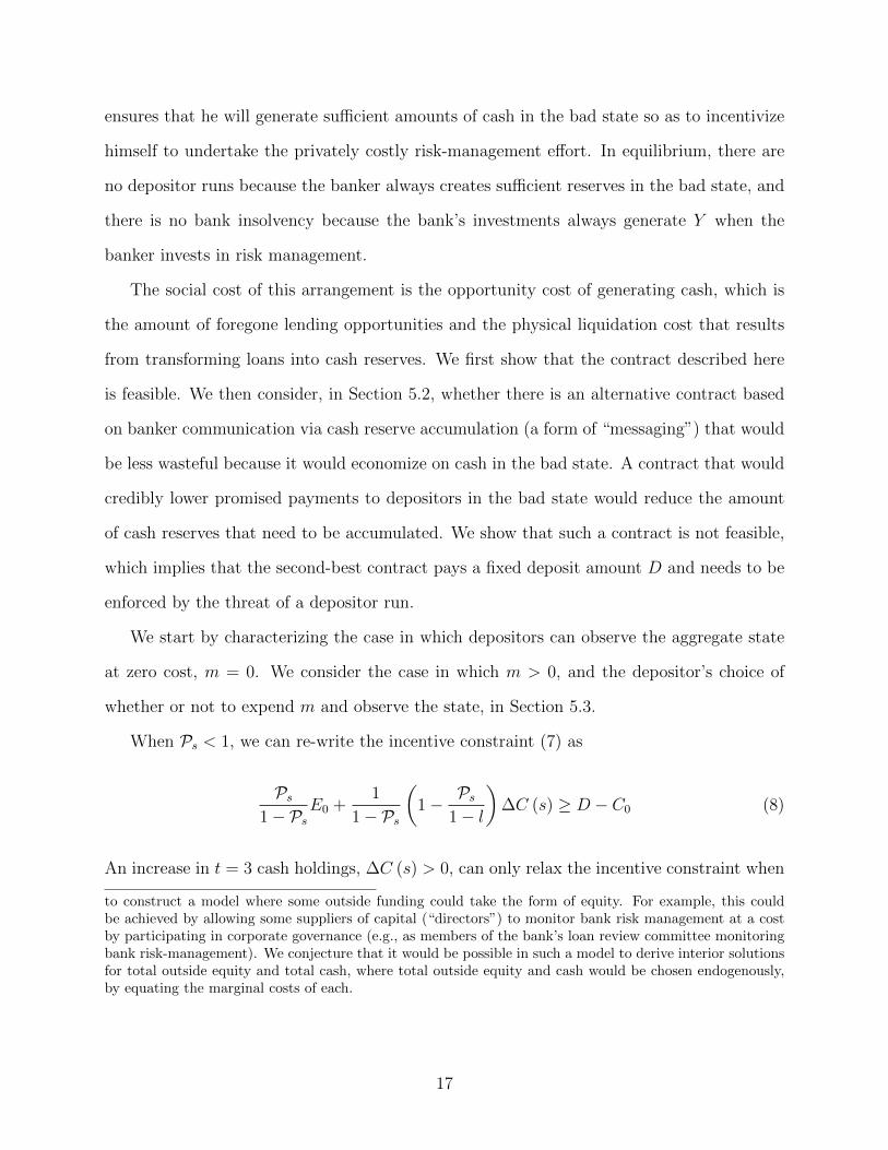
When Ps < 1, we can re-write the incentive constraint (7) as

Ps1− Ps

E0 +1

1− Ps

(1− Ps

1− l

)∆C (s) ≥ D − C0 (8)

An increase in t = 3 cash holdings, ∆C (s) > 0, can only relax the incentive constraint when

to construct a model where some outside funding could take the form of equity. For example, this couldbe achieved by allowing some suppliers of capital (“directors”) to monitor bank risk management at a costby participating in corporate governance (e.g., as members of the bank’s loan review committee monitoringbank risk-management). We conjecture that it would be possible in such a model to derive interior solutionsfor total outside equity and total cash, where total outside equity and cash would be chosen endogenously,by equating the marginal costs of each.

17

the term in brackets is positive, which is the case when

Ps < 1− l. (9)

Liquidating loans only helps with incentives when the liquidation return is higher than the

pledgeable return. Moreover, (8) implies that while both cash at t = 0 and extra cash at

t = 3 relax the incentive constraint, they do not have the same role in relaxing incentives.

C0 has a per unit benefit of one but is not contingent on the state. ∆C (s) is contingent on

the state (i.e., it is flexible), but its per unit benefit is less than one:

1

1− Ps

(1− Ps

1− l

)< 1.

In equilibrium, the banker always exerts effort, and his payoff from taking in deposits

and operating the bank is:

q [Y L3 (g) + C3 (g)−D] + (1− q) [Y L3 (b) + C3 (b)−D]

which, using L3 (s) = L0−∆C (s) 11−l , C3 (s) = C0 +∆C (s), and L0 = D+E0−C0, re-writes

as:

Y E0 + (Y − 1)(D − C0)−(

Y

1− l− 1

)[q∆C(g) + (1− q)∆C(b)] . (10)

The banker maximizes (10) subject to the incentive constraints (7) (one for each aggregate

state), the feasibility constraints D ≤ D and 0 ≤ ∆C(s) ≤ (1− l)(D+E0−C0), the banker’s

participation constraint (requiring that he does better by taking in deposits rather than by

investing only his own equity):

Y E0 + (Y − 1)(D − C0)−(

Y

1− l− 1

)[q∆C(g) + (1− q)∆C(b)] ≥ Y E0 (11)

and the no run condition for depositors requiring that (1− v)L3 (s) + C3 (s) ≤ D or, after

18

substituting for L3 (s) and C3 (s) and simplifying:

1− vv

E0 + ∆C (s)v − l

v (1− l)≤ D − C0. (12)

For ease of exposition, we will now consider the case in which there is no incentive problem

in the good aggregate state, Pg > 1, and in which the liquidation costs for depositors are

sufficiently high (see condition (13) below). Then, ∆C(g) = 0. At this point, it is useful to

introduce some notation. Define the net return on loans as r ≡ Y − 1, the outside financing

capacity of equity in the bad state as fb ≡ Pb

1−Pb, the ratio of return-to-cost of liquidation

for the banker as λ ≡ 1−ll

, and the ratio of return-to-cost of liquidation for depositors as

ν ≡ 1−vv

, with:8

ν < λ− (1− q)(

1 + r

r+ λ

). (13)

With this notation, we can now spell out our assumption about the maximum available

amount of deposits, D. We posit that

D

E0

< λ <λ+ fb1 + fb

. (14)

This assumption avoids an automatic liquidation of the bank in the bad aggregate state and

makes it impossible for bankers with severe moral hazard (low fb) to attract any deposits.

The following proposition summarizes the case when depositors can observe the aggregate

state at no cost.

Proposition 2 When risk-management effort is unobservable and the first-best is unattain-

able, the banker is incentivized to exert effort by holding cash. If

fb ≥ λ− (1− q)(

1 + r

r+ λ

)(15)

8This condition rules out a set of parameters for which deposit-taking is not feasible at intermediate levelsof financing capacity fb.

19

holds, then adjusting cash at t = 3 is too costly and the banker builds incentive-compatible

cash holdings at t = 0. If condition (15) does not hold and fb ≥ ν, then the banker increases

his cash holdings at t = 3 if the bad aggregate state is realized. For fb < ν, the banker will

not raise deposits and will invest solely his own equity.

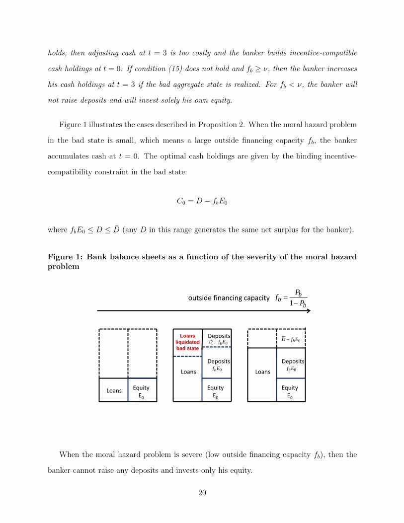
Figure 1 illustrates the cases described in Proposition 2. When the moral hazard problem

in the bad state is small, which means a large outside financing capacity fb, the banker

accumulates cash at t = 0. The optimal cash holdings are given by the binding incentive-

compatibility constraint in the bad state:

C0 = D − fbE0

where fbE0 ≤ D ≤ D (any D in this range generates the same net surplus for the banker).

Figure 1: Bank balance sheets as a function of the severity of the moral hazardproblem

Equity E0

Deposits

Loans

Loans liquidated bad state

Deposits 0EfD b−

0Efb

Equity E0

Loans

outside financing capacity

Equity E0

Deposits

Loans

0EfD b−

0Efb

b

bb P

Pf−

=1

When the moral hazard problem is severe (low outside financing capacity fb), then the

banker cannot raise any deposits and invests only his equity.

20

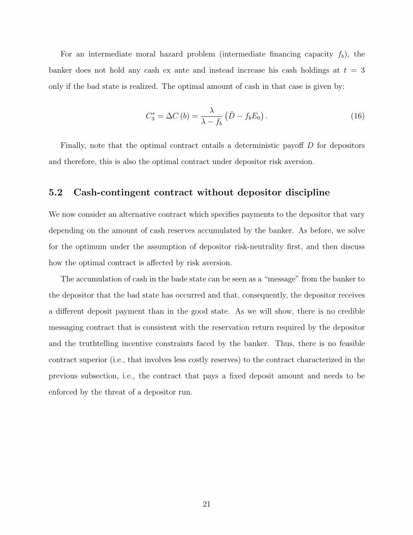
For an intermediate moral hazard problem (intermediate financing capacity fb), the

banker does not hold any cash ex ante and instead increase his cash holdings at t = 3

only if the bad state is realized. The optimal amount of cash in that case is given by:

C∗3 = ∆C (b) =λ

λ− fb(D − fbE0

). (16)

Finally, note that the optimal contract entails a deterministic payoff D for depositors

and therefore, this is also the optimal contract under depositor risk aversion.

5.2 Cash-contingent contract without depositor discipline

We now consider an alternative contract which specifies payments to the depositor that vary

depending on the amount of cash reserves accumulated by the banker. As before, we solve

for the optimum under the assumption of depositor risk-neutrality first, and then discuss

how the optimal contract is affected by risk aversion.

The accumulation of cash in the bade state can be seen as a “message” from the banker to

the depositor that the bad state has occurred and that, consequently, the depositor receives

a different deposit payment than in the good state. As we will show, there is no credible

messaging contract that is consistent with the reservation return required by the depositor

and the truthtelling incentive constraints faced by the banker. Thus, there is no feasible

contract superior (i.e., that involves less costly reserves) to the contract characterized in the

previous subsection, i.e., the contract that pays a fixed deposit amount and needs to be

enforced by the threat of a depositor run.

21

Consider the following deviation from the optimal contract with a fixed payment D:

Dg = D + ε

Db = D − εq

1− qCg = 0

Cb < C∗3 .

Note that the depositor participation constraint can be written as qDg + (1− q)Db = D.

That is, the deviation we consider satisfies the participation constraint of depositors if and

only if the promised payments are always made in each of the two states, i.e., the banker

exerts effort in the bad state (he always does in the good state by assumption). This will

occur if and only if the banker truthfully reveals the bad state through his selection of the

amount of reserves. The truth-telling constraints that must be satisfied consider whether the

banker is better off truthfully signaling the state (and specifying the contractual payment

accordingly) through his choice of reserves.

In the good state, the banker must get more value by not accumulating reserves:

Y L3(g)−Dg ≥ Y L3(b) + Cb −Db (17)

where L3(g) = L0 = D+E0 and L3(b) = L0−Cb 11−l = D+E0−Cb 1

1−l . (Recall that L3 only

depends on the announcement of the state but not the true state).

In the bad state, the truthtelling constraint is:

Y L3(b) + Cb −Db ≥ p (Y L3(g)−Dg) +BL3(g). (18)

Note that if the banker announces the good state even though it is the bad one, and thus

does not accumulate reserves, he will shirk on risk-management effort (because the promised

payment is too high relative to the accumulated reserves to elicit risk-management effort).

22

Hence, loans fail with probability p but he receives the private benefit B on each loan.

It turns out, that it is not optimal to save on cash reserves by offering a contract with

state-contingent deposit repayment but no ability to run.

Proposition 3 No deviation (ε, Cb) from the contract with fixed deposit repayment satisfies

the truth-telling constraints (17) and (18).

5.3 Aggregate State Observable at a Cost

In this subsection, we consider the case in which depositors can observe the aggregate state

at a cost m > 0. Hence, they have to decide whether or not it is in their interest to expend

this cost.

If depositors spend m and observe the aggregate state, then the solution to the banker’s

problem is the same as the one characterized in the previous subsection, except that the

promised payout to depositors has to be increased by m (so that depositors still break-even

on the contract, even though they have to pay m to observe the aggregate state). Hence,

the banker’s surplus is reduced by m.

If depositors decide not to spend m, then the solution to the banker’s problem is as

follows. Since depositors cannot distinguish the good aggregate state from the bad one, the

banker has to hold the same amount of cash in both states. The banker’s cash holdings have

to be high enough to ensure that he exerts risk-management effort in the bad aggregate state

(then, he would also exert effort in the good state). If the banker did not hold enough cash

to satisfy his incentive constraint in the bad state, the equilibrium with banking would not

be viable. It follows that the banker will find it optimal to satisfy his incentive constraint

with t = 0 cash only. This is because there is no flexibility benefit of increasing cash at t = 3

(since depositors cannot tell the states apart) and increasing cash holdings at t = 3 is always

more costly than building sufficient cash reserves at t = 0.

This logic leads to the following proposition.

23

Proposition 4 If the cost of observing the aggregate state m is low, depositors become in-

formed about the aggregate state and the banker increases his cash holdings if the bad aggregate

state realizes, as long as the liquidation is not too costly. If the cost m is high, depositors

do not become informed and the banker only uses cash at t = 0 as a commitment for proper

risk management.

6 Deposit Insurance

In the autarkic banking equilibria we have discussed thus far, banks choose the optimal

level of reserves voluntarily. We now consider an environment with heterogeneous banks in

which deposit insurance emerges as a part of the optimal contract. The deposit insurance

equilibrium entails social benefits as well as social costs. The benefit is insuring depositors

against the consequence of contracting with a weak bank. Cash reserve requirements are an

integral part of this deposit insurance equilibrium as they limit the social cost of insurance

by limiting the subsidy that weak banks extract from sound banks.

In the autarky set-up considered thus far, there is no purpose to deposit insurance. In

equilibrium (conditional on the incentive-compatible supply of risk-management effort by

bankers), all banks receive payout Y L3(s) at t = 5 and all depositors are paid the amount

D promised to them at t = 0 from those proceeds.

In order to motivate deposit insurance, we introduce heterogeneity in the banking system

which potentially creates an externality among banks.9 Specifically, we assume that some

9An alternative modeling approach would rely instead on political economy rather than efficiency tomotivate deposit insurance. For example, a subset of bankers might lobby for a deposit insurance systemthat subsidizes them at the expense of other banks. Politically influential “risky bankers” receive a cross-subsidy from low-risk bankers through the provision of deposit insurance. This approach to motivatingdeposit insurance is defensible on historical grounds. Federal deposit insurance began in the United Statesas the result of the Banking Act of 1933 (Calomiris and White 1994; Calomiris and Haber 2014, Chapter 6).It was understood by advocates and opponents to have resulted from special interest advocacy by small, riskyrural banks at the expense of other banks. President Roosevelt, Senator Carter Glass, the Federal Reserve,the Treasury and the American Bankers Association all opposed it, but acquiesced as part of a politicalcompromise with Representative Henry Steagall and others who championed the interests of small ruralbankers. The spread of deposit insurance internationally in the latter half of the twentieth century is alsounderstandable as a political process (Demirguc-Kunt, Kane and Laeven 2008). Furthermore, there is a large

24

fraction (α) of bankers have unobservably higher private cost of managing risk in the bad

state of the world (Bhb rather than Bb). We refer to banks whose private cost of risk manage-

ment is equal to Bb as “sound” banks and to those whose private cost of risk management

equal to Bhb as “weak” banks. We assume that Bh

b is sufficiently high so that weak banks

choose not to invest in risk management in the bad state of the world, i.e.,

Bhb > (1− p)Y. (19)

Because weak banks have a higher default probability in the bad state than sound banks,

and because the bank type is privately observed, this can create an externality between

banks. We show that one way to deal with this externality is for bankers to insure each other’s

deposits so that depositors receive a riskless payment even if their bank’s loan proceeds are

zero (Proposition 5). An alternative way is a contract in which all banks pay a risk premium

on deposits that compensates depositors for the risk associated with having deposited with

one of the weak bankers. We show that such a contract dominates deposit insurance under

risk neutrality. However, for a sufficiently large depositor risk-aversion, the deposit insurance

equilibrium dominates the equilibrium without deposit insurance (Proposition 6).

6.1 The Deposit Insurance Equilibrium

In the deposit insurance equilibrium, banks agree to provide deposit insurance to one another

so that the banks that forego risk management and earn a zero return at t = 5 will have their

promised deposit payments covered by surviving banks. A condition for receiving deposit

insurance is a bank’s willingness to hold the amount of required reserves established by the

deposit insurance system.

Referring to Proposition 2, we assume, without loss of generality, that liquidation costs

literature establishing that risk subsidization has been a predictable consequence of most deposit insurancearrangements around the world (Demirguc-Kunt and Detragiache 2002, Demirguc-Kunt and Huizinga 2004,Cull, Senbet and Sorge 2005).

25

are low enough so that reserves are accumulated only at t = 3. As before, the state is not

contractible. Furthermore, unlike the uninsured depositors in Section 5, who are willing

to invest resources to observe the state, insured depositors no longer have an incentive to

monitor the state to ensure that banks top up their cash reserves in the bad state. However,

sound banks who wish to participate in the deposit insurance system with a cash reserve

requirement can now be relied upon to truthfully reveal the bad state, which entails that all

banks participating in the deposit insurance system accumulate reserves of C∗3 at t = 3 (given

in (16)). Their announcements of the bad state are reliable because they benefit individually

from identifying the bad state if and only if it occurs, given their liability for insuring the

depositors of failed weak banks. The revelation of the bad state can be implemented by

specifying a rule saying that if any bank that is a member of the deposit insurance system

claims that the bad state has occurred, it will be deemed to have occurred.

We first consider the case of a pooling equilibrium in which both types of banks (Bb, Bhb )

choose to participate in the deposit insurance scheme. We derive conditions under which

pooling occurs. We assume that any deviation from equilibrium behavior is interpreted as

coming from a weak bank.

Let us consider the behavior of sound banks (Bb) first. Sound banks will have to bail out

the deposits of weak banks when the bad state and the bad outcome occur. By assumption

(19), weak banks will not choose to invest in risk management in bad states of the world

because Bhb is sufficiently high. The aggregate expected cost of insuring weak banks’ deposits

in the bad state is:

d = α(1− p)(D − C∗3),

which is the product of the proportion of expected weak bankers at t = 0, the probability of

the bad outcome, and the amount of deposit liabilities of weak banks in excess of their cash

reserves. A sound banker is willing to participate in deposit insurance as long as his payoff

26

from doing so is higher than his payoff from not participating in deposit insurance:

[qY L3(g) + (1− q)(Y L3(b) + C∗3)−D]− (1− q) d

(1− α) + αp≥ Y E0. (20)

The left-hand side is a sound banker’s profit from running a bank minus the expected cost

of participating in deposit insurance. The deposit insurance cost d must be paid in the bad

state (which occurs with probability 1 − q) and 1(1−α)+αp

is each sound bank’s share of the

deposit insurance cost. Note that αp proportion of the weak banks will survive and share the

bailout costs with the sound banks. If a sound banker chooses not to participate in deposit

insurance (right-hand side of (20)), depositors believe that he is a weak banker and therefore

do not deposit in his bank (recall that, by assumption (1), it is not worthwhile for depositors

to fund a bank that they know does not engage in risk management in both states). Hence,

the banker invests solely his own equity and obtains Y E0.

Weak banks (Bhb ) will also be willing to participate in the deposit insurance equilibrium

as long as doing so is profitable for them. The condition can be written, for a particular

weak bank, as:

q[Y L3(g)−D] + (1− q)p[Y L3(b) + C∗3 −D −

d

(1− α) + αp

]+ (1− q)Bh

bL3(b) ≥ E0. (21)

The left-hand side is a weak banker’s profit from running a bank and pooling with sound

bankers. In the good state (which occurs with probability q), weak banks do risk management

and repay their depositors. In the bad state (which occurs with probability 1−q), weak banks

do not manage risk and therefore earn private benefit Bhb per unit of their loans L3(b). A p

proportion of weak banks generates the return Y on loans, repays their depositors and shares

the bailout costs d. The rest of the weak banks fail to generate a positive return on the loans

and are only left with the reserves C∗3 . Those reserves are used to pay off their depositors,

and the shortfall D−C∗3 is then covered by the deposit insurance. The right-hand side of (21)

is the payoff a weak banker earns when not participating in the deposit insurance. In this

27

case, he is identified as a weak banker and therefore cannot attract any deposits (assumption

(1)). The payoff of a weak bank when not joining the deposit insurance is E0. He does not

make loans because they have negative NPV as he does not exert risk-management effort.

We can now state the condition under which both sound and weak banks are willing to

participate in deposit insurance.

Proposition 5 Both sound banks and weak banks are willing to participate in a deposit

insurance system in which pooling occurs if the good state is sufficiently likely (q is sufficiently

high). Sound banks will truthfully declare the bad state when it occurs, thereby requiring that

all banks accumulate reserves C∗3 .

For completeness, we mention properties of a separating equilibrium in which sound

banks are willing to participate in deposit insurance while weak banks are not willing to

participate. In this case, the willingness to participate in deposit insurance signals sound

bank quality. Obviously, sound banks are willing to participate in deposit insurance because

in so doing they achieve separation and therefore avoid any cost of subsidizing weak banks.

This equilibrium is the same as in the model without weak banks.

6.2 Optimality of deposit insurance

Here we show that the deposit insurance pooling equilibrium is not dominated by a pooling

equilibrium without deposit insurance as long as depositors are sufficiently risk averse. When

depositors are sufficiently risk-averse, both sound banks and weak banks will prefer the

deposit insurance pooling equilibrium to pooling without deposit insurance. Both types of

banks earn more rents from pooling with deposit insurance.

If there is pooling without deposit insurance, then risk-neutral depositors are willing to

accept a higher payment (D + ε) when their bank is solvent in order to compensate them

for the loss when their bank is insolvent. The higher payment is given by the depositor

28

participation constraint:

[(1− α) + αq + αp(1− q)](D + ε) + (1− q)(1− p)αC∗3 = D. (22)

In words, without deposit insurance, depositors earn the promised payment (D + ε) if

they are lucky enough to deposit with a sound bank, or if they deposit with a weak bank in

the good state, or if they deposit with the weak bank in the bad state but are lucky enough

for the good outcome to occur. When none of those is true, they receive only C∗3 .

In pooling without deposit insurance, sound banks no longer have to pay their share of

the deposit obligations of failed weak banks, but they do have to pay their own depositors

more as the result of the inability of depositors to distinguish sound from weak banks. In

the pooling equilibrium without deposit insurance, each sound bank will earn rent equal to:

qY L3(g) + (1− q)(Y L3(b) + C∗3)− (D + ε)− Y E0.

Proposition 6 Suppose q is sufficiently high so that both sound and weak banks are willing

to participate in a deposit insurance system with pooling. If depositors are sufficiently risk

averse, then pooling with deposit insurance is optimal.

7 Mutual Liquidity Risk Insurance

We now relax the assumption made in the prior sections of the paper to permit depositors

also to make exogenous withdrawals at t = 1 in response to a need for liquidity that is

unrelated to the condition of banks. Specifically, we assume that at t = 1, each bank is

subject to an exogenous liquidity shock, which is i.i.d. across banks. As before, we assume,

without loss of generality, that liquidation costs are low enough so that for the purpose

of ensuring credible risk-management effort, banks only accumulate cash reserves at t = 3

(Proposition 2). In the presence of exogenous liquidity risk, which occurs at t = 1, banks

29

must, however, also accumulate cash reserves at t = 0.

We show that adding this feature to the model results in bank coinsurance of the liquidity

risk related to exogenous withdrawals of deposits. As part of the coinsurance arrangements

among banks, bankers will require one another to maintain cash reserves to avoid free-riding

on the collective coinsurance of exogenous liquidity risk. This is true whether or not the

deposit insurance exists, and therefore provides an independent motivation for cash reserve

requirements.

For tractability, we assume that the size of the liquidity shock is identical across banks.

With probability π, each bank experiences a withdrawal of a fraction µ of its deposits (D)

at t = 1, and with probability (1− π), each bank experiences zero exogenous withdrawals of

deposits at t = 1.

We interpret the exogenous liquidity shock as a withdrawal necessitated by a bank de-

positor’s need to purchase an item of value µD from “abroad.” The international feature of

the transfer has important consequences for the cash needs of banks. In our model, unlike

other models of liquidity demand shocks in banking (such as Diamond and Dybvig 1983) we

do not assume that shocks to depositor’s desire to purchase goods and services necessarily

result in disintermediation. In our model, “domestic” transfers among individual depositors

would not require the physical interbank exchange of cash. Depositors’ domestic purchases

can be accomplished by interbank accounting transfers of deposits among the banks within

the domestic banking system because, in equilibrium, banks have an incentive to agree to

offset any individual deposit flows with countervailing interbank deposit flows at t = 1. This

can be accomplished without any transfer of cash. When a depositor makes a domestic

purchase of µD, she uses a check drawn on her bank (Bank A) to execute that purchase.

The seller of the domestic good deposits that check in his bank (Bank B), and an offsetting

interbank accounting transaction can occur (a deposit claim of Bank B on Bank A for µD),

which balances the books between the banks to take account of and offset the individual

deposits being debited and credited at the two banks. This is feasible because the domestic

30

transaction is observable to the domestic banks (i.e., the transaction is routed through the

clearing house owned by all the banks collectively).

Because the source of domestic interbank transfers is observably exogenous to any banker’s

decisions, and because there is no moral hazard arising as the result of any change in any

bank’s balance sheet (the bank losing deposit dollars experiences no net change in its to-

tal deposits, which consist of the sum of individual plus interbank deposits; and similarly

the bank receiving the deposits experiences no net change in deposits), there is no need for

domestic banks to limit their willingness to offset individual domestic deposit flows with

interbank deposit flows. Depositors’ domestic purchases, therefore, will not necessitate any

cash transfers among domestic banks at t = 1, or any cash reserve holdings at t = 0.

In contrast, transfers of funds abroad occur outside of the domestic banking system. We

assume (on the basis of unspecified factors that limit international contracting) that it is

not physically possible for interbank deposits to offset international flows among individual

depositors. Thus, international transactions necessitate cash disbursements abroad by banks

experiencing an outflow of individual deposits.10

Domestic banks can benefit from coinsuring one another against liquidity shocks involving

international transactions. Those shocks are i.i.d. across banks, implying that, by the law

of large numbers, the amount of reserve outflows is πµD. Domestic banks will agree to the

following mutually beneficial arrangement: each bank holds πµD in cash reserves at t = 0.

All banks that experience international withdrawals of deposits can request a zero-interest

loan of cash from all the other banks in the amount (1−π)µD. The proceeds of this interbank

loan to any requesting bank is channeled through the clearing house at t = 1, which combines

the interbank loan proceeds of the lending banks of (1−π)µD with the borrowing bank’s own

holdings of πµD, and sends µD abroad to fund the transfers of cash to foreign banks that

are receiving international deposit inflows from the domestic bank members of the clearing

10This could take place, for example, via a transfer of gold balances from Bank A to a foreign bank, whichcould be accomplished through the export of gold, or the transfer of Bank A’s gold holdings already locatedin an account based abroad.

31

house. The loan is repaid by the disbursing bank at t = 5. Because the loan is riskless in

equilibrium, and because there is nothing to be gained by establishing rules that would limit

banks’ demands for liquidity, interbank loans for funding liquidity disbursements at t = 1

are given at a zero interest rate.

Two aspects of our assumptions relating to this arrangement, and the role of the clearing

house, should be emphasized. First, we assume that the clearing house can enforce the

reserve requirements credibly because it can monitor member banks’ holdings of cash and

require members to maintain a cash balance of πµD at t = 0. Second, because the clearing

house aggregates the interbank loans of cash at t = 1 and sends them abroad as agent for

the disbursing banks, there is no moral hazard associated with deception by the bank that is

sending the gold abroad. If the clearing house was not acting as agent for the transfer, then

one could worry that domestic banks might have an incentive to overstate their needs for

gold transfers. By doing so they could obtain gold at t = 1 (at the expense of other banks’

foregone opportunity costs from lending) which would reduce that bank’s cost of maintaining

reserve holdings at t = 3 to avoid the threat of a deposit run if the bad state occurs.

Because banks coinsure the liquidity risk of withdrawals abroad, each bank’s total debt

(consisting of customer plus interbank deposits) falls by πµD at t = 1. Because D is the

binding constraint on the scale of banks, the existence of the liquidity shock implies that L0

will be slightly lower (by the amount πµD) than in the equilibrium where π = 0.11

Note that in our framework we separate the timing of the exogenous liquidity shock

from the timing of other events. Exogenous transfers abroad occur prior to the revelation

of the state (which occurs at t = 2), prior to bankers’ decisions about “topping up” cash

balances and the endogenous withdrawals by depositors (at t = 3), and prior to any risk-

management action by bankers (at t = 4). Cash reserves used to satisfy foreign needs flow

out at t = 1. Our results do not depend crucially on this timing convention. By assuming

that exogenous withdrawals precede endogenous withdrawals, we are able to model their

11Note that because L0 is lower than before, the amount of loans that must be liquidated in the bad stateat t = 3 is also lower than before.

32

consequences for reserve balances as independent. If, however, the sequencing of the two

sources of deposit withdrawal (exogenous and endogenous withdrawals) were reversed, the

amounts of reserves held for the two purposes would not always be independent. For example,

reserves accumulated by banks in response to the revelation of the bad state could be available

(once risk-management decisions have been made) to fund international transfers of cash.

This scope economy, however, complicates the analysis while not affecting the key results of

the model.

Consistent with Proposition 2, in a model where π = 0 (that is, a model without exoge-

nous liquidity risk), under some parameterizations of our model (e.g., when l is high), banks

will choose to maintain positive reserves at t = 0 in order to avoid the costs of “topping

up” at t = 3. In that case the clearing house will require that banks hold C∗0 + πµD, where

C∗0 is the amount of reserves banks choose to hold in the absence of the exogenous liquidity

shock.12

8 Conclusion

We consider the role that cash reserves play in optimal banking arrangements. Cash re-

serves reduce the vulnerability of banks to liquidity risks that arise from granting depositors

the option to withdraw their funds. Liquidity risk is of two types, exogenous (where with-

drawal behavior is unrelated to depositors’ beliefs about bank conditions) and endogenous

(where withdrawals reflect deterioration in bank conditions). The role of cash in mitigating

exogenous liquidity risk is straightforward: holding cash sufficient to cover exogenous un-

predictable needs of depositors makes it possible to avoid destabilizing bank failures or high

12Thus far, the aggregate amount of liquidity that needs to be withdrawn from the banking system hasbeen fixed at µD. We could allow for the possibility of an adverse systemic shock: In addition to µD, withprobability φ, an amount x must be shipped abroad by each bank. Banks can deal with this risk in one oftwo ways. They could either maintain additional cash reserves at t = 0 in the amount x or liquidate loansat t = 1 to generate sufficient cash when the systemic shock is realized. Similar to the logic underlyingProposition 2, which of these solutions the banks choose will depend on the costs of liquidation l and theprobability φ. In states where the systemic shock occurs, banks will experience a reduction in deposits att = 1, and therefore, the amount of liquidation needed at t = 3 in the bad state will be less than in themodel without systemic liquidity risk.

33

liquidation costs of loan portfolios that would occur in the absence of cash.

In the case of endogenous liquidity risk, the role of cash is to reduce insolvency risk

by incentivizing efficient risk management by bankers. The fact that cash is impervious to

moral hazard makes its possession by banks (e.g., in the form of deposits at the central

bank) uniquely useful in promoting good risk management by banks with respect to their

risky assets. Banks that hold sufficient cash are able to gain market confidence in their

risk management, and thereby attract and retain deposits. In bad states of the world (i.e.,

recessions) banks that might otherwise be tempted to allow risky assets to become riskier

will raise their cash holdings to preserve market confidence in their low risk. The use of cash

in our model expands efficient bank lending.

We begin with autarkic models of single banks and their optimal contracts with depos-

itors. In such environments, although cash reserves play a crucial role in bank contracting,

there is no need for cash reserve requirements imposed either by a coalition of banks or by

the government. Individual banks face the incentive to offer optimal contracts that create

the incentive for them to maintain cash reserves.

Once we allow for heterogeneity among multiple banks, however, cash reserve require-

ments – imposed either by private coalitions of banks or by the government – become neces-

sary as a means of preventing free riding on collective protection. In the case of endogenous

liquidity risk, in an environment where banks are of heterogeneous quality, and where de-

positors are sufficiently risk averse, deposit insurance arises as part of the optimal banking

contract because it insulates depositors from the consequences of bank heterogeneity. In that

environment, a cash reserve requirement is needed to limit the extent of the subsidy weak

banks receive from sound banks.

In the case of exogenous liquidity risk, in an environment where banks can benefit from

coinsuring each other’s diversifiable liquidity risk, a cash reserve requirement is necessary to

prevent free riding on other banks and thereby make collective protection credible.

Our model points to important shortcomings in existing regulatory frameworks for liquid-

34

ity requirements, such as Basel III. That framework’s liquidity standards view reductions in

short-term debt as interchangeable with increases in cash reserves. In contrast, in our model,

the combination of a large amount of short-term debt and a high cash reserve requirement

is efficient and superior to a regulatory rule that would encourage lower levels of both.

35

References

[1] Besanko and A. Thakor (1987). “Competitive Equilibrium in the Credit Market underAsymmetric Information,” Journal of Economic Theory 42, 167-182.

[2] Boot, A., and A. Thakor (1994). “Moral Hazard and Secured Lending in an InfinitelyRepeated Credit Market Game,” International Economic Review 35, 899-920.

[3] Biais, B., F. Heider, and M. Hoerova (2012). “Risk-sharing or Risk-taking? Counter-party Risk, Incentives, and Margins,” ECB Working Paper No. 1413.

[4] Basel Committee on Banking Supervision (2013). Basel III: The Liquidity CoverageRatio and Liquidity Risk Monitoring Tools, Bank for International Settlements.

[5] Calomiris, C. W. (1990). “Is Deposit Insurance Necessary? A Historical Perspective,”Journal of Economic History, June, 283-295.

[6] Calomiris, C. W., and G. Gorton (1991). “The Origins of Banking Panics: Models,Facts, and Bank Regulation,” in Financial Markets and Financial Crises, R. GlennHubbard, ed., NBER, University of Chicago Press, 109-173.

[7] Calomiris, C. W., and S. H. Haber (2014). Fragile By Design: The Political Origins ofBanking Crises and Scarce Credit, Princeton University Press.

[8] Calomiris, C. W., and R. Herring (2013). “How to Design a Contingent ConvertibleDebt Requirement that Helps Solve Our Too-Big-To-Fail Problem,”Journal of AppliedCorporate Finance 25, 21-44.

[9] Calomiris, C. W., and C. M. Kahn (1991). “The Role of Demandable Debt in StructuringOptimal Banking Arrangements,” American Economic Review 81, 497-513.

[10] Calomiris, C. W., and E. N. White (1994). “The Origins of Federal Deposit Insurance,”in C. Golding and G. Libecap (eds), The Regulated Economy: A Historical Perspective,University of Chicago Press.

[11] Covitz, D., N. Liang, and G. Suarez (2013). “The Evolution of a Financial Crisis:Collapse of the Asset-Backed Commercial Paper,” Journal of Finance 68, 815-848.

[12] Cull, R., L. Senbet, and M. Sorge (2005). “Deposit Insurance and Financial Develop-ment,” Journal of Money, Credit and Banking 37, 43-82.

[13] Demirguc-Kunt, A., and E. Detragiache (2002). “Does Deposit Insurance Increase Bank-ing System Stability? An Empirical Investigation,” Journal of Monetary Economics 49,1373-1406.

[14] Demirguc-Kunt, A., and H. Huizinga (2004). “Market Discipline and Deposit Insur-ance,” Journal of Monetary Economics 51, 375-99.

[15] Demirguc-Kunt, A., E. J. Kane, and L. Laeven (2008). Deposit Insurance Around theWorld: Issues of Design and Implementation, MIT Press.

36

[16] Diamond , D. (1984). “Financial Intermediation and Delegated Monitoring,” Review ofEconomic Studies 51, 393-414.

[17] Diamond, D., and P. Dybvig (1983). “Bank Runs, Deposit Insurance, and Liquidity,”Journal of Political Economy 91, 401-419.

[18] Diamond, D., and R. Rajan (2001). “Liquidity Risk, Liquidity Creation, and FinancialFragility: A Theory of Banking, ” Journal of Political Economy 109, 287-327.

[19] Ellul, A., and V. Yerramilli (2013). “Stronger Risk Controls, Lower Risk: Evidence fromU.S. Bank Holding Companies,” Journal of Finance 68, 1757-1803.

[20] Fahlenbrach, R., Prilmeier, R., and R. Stulz (2012). “This Time Is the Same: UsingBank Performance in 1998 to Explain Bank Performance during the Recent FinancialCrisis,” Journal of Finance 67, 2139-2185.

[21] Gale, D., and M. Hellwig (1985). “Incentive-Compatible Debt Contracts: The One-Period Problem,” Review of Economic Studies 52, 647-663.

[22] Goodhart, C. (2008). “Liquidity Risk Management,” Banque de France Financial Sta-bility Review – Special Issue on Liquidity, February, 39-44.

[23] Gorton, G. (1985). “Clearinghouses and the Origin of Central Banking in the U.S.,”Journal of Economic History 45, 277-283.

[24] Gorton, G. and A. Metrick (2012). “Securitized Banking and the Run on Repo,” Journalof Financial Economics 104, 425-451.

[25] Gorton, G., and G. Pennacchi (1990). “Financial Intermediaries and Liquidity Cre-ation,” Journal of Finance 45, 49-71.

[26] Heider, F., M. Hoerova, and C. Holthausen (2009). “Liquidity Hoarding and InterbankMarket Spreads: The Role of Counterparty Risk,” ECB Working Paper No. 1126.

[27] Holmstrom, B. and J. Tirole (1997). “Financial Intermediation, Loanable Funds, andthe Real Sector,” Quarterly Journal of Economics 112, 663-692.

[28] Holmstrom, B. and J. Tirole (1998). “Private and Public Supply of Liquidity,” Journalof Political Economy 106, 1-40.

[29] Merton, R. C. (1977). “On the Pricing of Contingent Claims and the Modigliani-MillerTheorem,” Journal of Financial Economics 5, 241-249.

[30] Myers, S., and N. Majluf (1984). “Corporate Financing and Investment Decisions whenFirms Have Information that Investors Do Not Have,” Journal of Financial Economics13, 187-222.

[31] Myers, S., and R. Rajan (1998). “The Paradox of Liquidity,” Quarterly Journal ofEconomics 113, 733-771.

37

[32] Rajan, R. (1992). “Insiders and Outsiders: The Choice between Informed and Arm’s-Length Debt,” Journal of Finance 47, 1367-1400.

[33] Townsend, R. (1979). “Optimal Contracts and Competitive Markets with Costly StateVerification,” Journal of Economic Theory 21, 265-293.

[34] Weidmann, J. (2014). “Stable Banks for a Stable Europe,” Speech at the 20th GermanBanking Congress, April 7.

[35] Wicker, E. (2000). Banking Panics of the Gilded Age, New York: Cambridge UniversityPress.

38

9 Appendix

Proof of Proposition 2 The incentive constraint in the bad aggregate state must bebinding since cash holdings are costly and hence the banker will choose to hold just enoughcash to satisfy the incentive constraint. The binding incentive constraint in the bad state(8) can be written as:

fbE0 +λ− fbλ

∆C (b) = D − C0. (23)

Note that the no-run condition (12) can be written as:

νE0 +λ− νλ

∆C (b) ≤ D − C0. (24)

From (10), we get that the net surplus of the banker (over the return from investing onlyhis own equity, Y E0) is given by:

r(D − C0)− (1− q)1 + r + rλ

λ∆C(b). (25)

Substituting the binding incentive constraint (23) into (25) yields:

rfbE0 +

[λ− fbλ

r − (1− q)1 + r + rλ

λ

]∆C(b). (26)

It follows that if the expression in the square brackets above is non-positive,

λ− fbλ

r − (1− q)1 + r + rλ

λ≤ 0

or, equivalently,

fb ≥ λ− (1− q)(

1 + r

r+ λ

), (27)

then the banker will never increase his cash holdings at t = 3 since his surplus is decreasingin ∆C.

Suppose condition (27) holds. From the binding incentive constraint (23), we get that:

fbE0 = D − C0 (28)

It follows that no run condition (24) is satisfied since fbE0 = D−C0 > νE0 holds by (27) and(13). By (26), the banker’s surplus in this case is given by rfbE0. Note that cash holdingsdo not affect the banker’s surplus since he only earns the net return r on loans. Hence, whencondition (27) holds, the banker will raise deposits and invest L0 = E0 + fbE0 into loans.He can raise deposits beyond fbE0 (the financing capacity of his equity in the bad state) aslong as he invests the extra deposits into cash at t = 0 so that the incentive constraint (28)continues to hold.

Suppose condition (27) does not hold. As the banker’s surplus (26) is increasing in∆C (b) in this case, the banker would want to set ∆C (b) as high as possible. From the

39

binding incentive constraint (23), we get:

∆C (b) =λ

λ− fb(D − C0 − fbE0) (29)

To make ∆C (b) as high as possible, the banker will set D = D and C0 = 0. Hence,∆C (b) = λ

λ−fb

(D − fbE0

). By (14), the banker will not liquidate all the loans as he will

exhaust the available deposits D before full liquidation. That is, ∆C (b) < (1− l) (D + E0)holds. Lastly, we check that that the no run condition (24) is satisfied. Substituting for∆C (b), D, and C0 in (24), we have that:

ν − fbλ− fb

[D − λE0

]≥ 0 (30)

must hold. Since we assume that D ≤ λE0, the equilibrium with deposit-taking is onlyviable for fb ≥ ν, i.e., when the banker has a sufficiently high financing capacity of the insideequity compared to the liquidation return of depositors. For fb < ν, the banker will not raisedeposits and will run the bank using his own equity only.

Proof of Proposition 3Substituting the values of (Dg, Cg) and (Db, Cb) into the truth-telling constraints and

rearranging yields:

Cb ≥ ε

(1

1− q

)(1

Y1−l − 1

)and

Cb ≤ ε

(q

1− q− p)(

1Y

1−l − 1

)+ (1− p)

(Pb (D + E0)−D

Y1−l − 1

).

We know that C∗3 > 0, which from the binding incentive constraint implies that Pb (D + E0)−D < 0. To see why, note that the incentive constraint (8) can be written as(

1− Pb1− l

)C∗3 = D − Pb(D + E0),

where we know that Pb < 1− l.Moreover, since 1

1−q >q

1−q − p always holds, there is no combination of Cb and ε thatsatisfies both truthtelling constraints.

Proof of Proposition 5Recall that we are considering the set of parameters such that liquidation costs are low

enough so bankers do not use ex ante cash, C0 = 0:

1− vv≤ fb < λ− (1− q)

[1 + r

r+ λ

]

40

Therefore, we have:

C∗3 = C0 + ∆C (b) = ∆C (b) =λ

λ− fb(D − fbE0

)where fb = Pb

1−Pband λ = 1−l

l. Furthermore,

D = D

L3(g) = E0 + D

L3(b) = L0 −∆C (b)1

1− l= E0 + D − C∗3

1

1− l= E0 + D − 1

λ− fb1

l

(D − fbE0

)For a weak banker, we need to show that

q[Y L3(g)−D] + (1− q)p[Y L3(b) + C∗3 −D −

d

(1− α) + αp

]+ (1− q)Bh

bL3(b) ≥ E0

Substituting for D, L3(g), L3(b) and d, and collecting terms, this is equivalent to showingthat:

[qY + (1− q)

(pY +Bh

b

)− 1]E0+

[q (Y − 1) + (1− q)

(p (Y − 1) +Bh

b

)− αp(1− p)(1− q)

(1− α) + αp

]D

− (1− q)[pY +Bh

b

1− l− p

(1− α) + αp

]C∗3 ≥ 0

Substituting for C∗3 and collecting terms, this is equivalent to showing that:[qY + (1− q)

(pY +Bh

b

)− 1 + (1− q) λfb

λ− fb

(pY +Bh

b

1− l− p

(1− α) + αp

)]E0+[

q (Y − 1)− (1− q)(pY +Bh

b

1− lfb + l (λ− fb)

(λ− fb)− p

(1− α) + αp

fbλ− fb

)]D ≥ 0

Putting together terms multiplied by (1− q) fbλ−fb

yields:

(qY + (1− q)

(pY +Bh

b

)− 1)E0 + q (Y − 1) D

+ (1− q) fbλ− fb

(pY +Bh

b

1− l− p

(1− α) + αp

)(λE0 − D

)− (1− q)

(pY +Bh

b

) Dλ

Note that the first term is positive,

qY + (1− q)(pY +Bh

b

)− 1 > 0

since pY + Bhb > pY + (1− p)Y > 1 (assumption (19)). The second term is also positive

as Y > 1. The third term is positive sincepY+Bh

b

1−l > 1 while p(1−α)+αp

< 1, and λE0 > D by

assumption (14). So, all terms above are positive except the last one. Using E0 >Dλ

, we

41

have (qY + (1− q)

(pY +Bh

b

)− 1)E0 + q (Y − 1) D

+(1− q) fbλ− fb

(pY +Bh

b

1− l− p

(1− α) + αp

)(λE0 − D

)− (1− q)

(pY +Bh

b

) Dλ>

(qY − 1)D

λ+ q (Y − 1) D + (1− q) fb

λ− fb

(pY +Bh

b

1− l− p

(1− α) + αp

)(λE0 − D

)=(

q (Y − 1) +1

λ(qY − 1)

)D + (1− q) fb

λ− fb

(pY +Bh

b

1− l− p

(1− α) + αp

)(λE0 − D

)As argued above, the second term is positive. A sufficient condition for the first term to bepositive is qY > 1 which holds for q sufficiently high (since Y > 1).

For a sound bank, we need to show that

[qY L3(g) + (1− q)(Y L3(b) + C∗3)−D]− (1− q) d

(1− α) + αp≥ Y E0

Substituting for D, L3(g), L3(b) and d, and collecting terms, this is equivalent to showingthat:

(Y − 1) D + (1− q)C∗3 − (1− q) Y

1− lC∗3 − (1− q) α(1− p)

(1− α) + αp

(D − C∗3

)≥ 0. (31)

The first three terms on the left-hand side of (31) give the net profit of a sounds bankerif he does not participate in the deposit insurance: the return on the loan-making activity(Y − 1) D, the return on cash holdings in the bad state (1 − q)C∗3 , net of the opportunitycost of liquidating loans in the bad state, (1 − q) Y

1−lC∗3 . The last term is the cost of the

deposit insurance to be paid in the bad state.Clearly, for q → 1 (or α → 0), (31) is satisfied, as deposit insurance costs vanish.

Moreover, the left-hand side of (31) is continuous (and increasing) in q. By continuity, (31)is satisfied for q sufficiently close to 1.

Therefore, for a q sufficiently close to 1, both weak and sound bankers are willing toparticipate in the deposit insurance.

Proof of Proposition 6 By the depositor participation constraint (22), we have that

ε =(1− q) d

1− α(1− p)(1− q)

under depositor risk-neutrality. By (20), a sound banker’s cost of participating in deposit

insurance is given by (1−q)d(1−α)+αp

. Thus, under risk neutrality, the cost of participating is greaterthan ε. In order for deposit insurance to be preferred, risk aversion must be large enoughsuch that ε > (1−q)d

(1−α)+αp.

42