Embed Size (px)
Citation preview
"A Theory of Financing Constraints and FirmDynamics"
G.L. Clementi and H.A. Hopenhayn (QJE, 2006)
Cesar E. TamayoEcon612- Economics - Rutgers
April 30, 2012
1/21

Program
I SummaryI Physical environmentI The contract design problemI Characterization of the optimal contractI Firm growth and survivalI Contract maturity and debt limits
2/21
What they do in a nutshell
I The paper develops a theory of endogenous �nancing constraints.
I Repeated moral hazard problemI The optimal contract (under asymmetric info) determines non-trivialstochastic processes for �rm size, equity and debt.
I This in turn implies non-trivial �rm dynamics even under simple i.i.d.shocks.
3/21
What they do in a nutshell
I The paper develops a theory of endogenous �nancing constraints.I Repeated moral hazard problem
I The optimal contract (under asymmetric info) determines non-trivialstochastic processes for �rm size, equity and debt.
I This in turn implies non-trivial �rm dynamics even under simple i.i.d.shocks.
3/21
What they do in a nutshell
I The paper develops a theory of endogenous �nancing constraints.I Repeated moral hazard problemI The optimal contract (under asymmetric info) determines non-trivialstochastic processes for �rm size, equity and debt.
I This in turn implies non-trivial �rm dynamics even under simple i.i.d.shocks.
3/21
Physical environment:
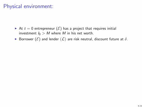
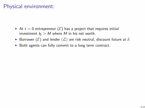
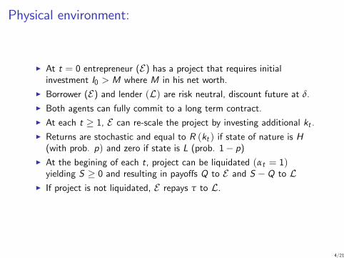
I At t = 0 entrepreneur (E) has a project that requires initialinvestment I0 > M where M in his net worth.
I Borrower (E) and lender (L) are risk neutral, discount future at δ.
I Both agents can fully commit to a long term contract.I At each t � 1, E can re-scale the project by investing additional kt .I Returns are stochastic and equal to R (kt ) if state of nature is H(with prob. p) and zero if state is L (prob. 1� p)
I At the begining of each t, project can be liquidated (αt = 1)yielding S � 0 and resulting in payo¤s Q to E and S �Q to L
I If project is not liquidated, E repays τ to L.
4/21
Physical environment:
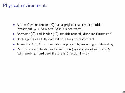
I At t = 0 entrepreneur (E) has a project that requires initialinvestment I0 > M where M in his net worth.
I Borrower (E) and lender (L) are risk neutral, discount future at δ.
I Both agents can fully commit to a long term contract.
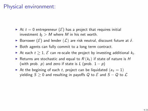
I At each t � 1, E can re-scale the project by investing additional kt .I Returns are stochastic and equal to R (kt ) if state of nature is H(with prob. p) and zero if state is L (prob. 1� p)
I At the begining of each t, project can be liquidated (αt = 1)yielding S � 0 and resulting in payo¤s Q to E and S �Q to L
I If project is not liquidated, E repays τ to L.
4/21

Physical environment:
I At t = 0 entrepreneur (E) has a project that requires initialinvestment I0 > M where M in his net worth.
I Borrower (E) and lender (L) are risk neutral, discount future at δ.
I Both agents can fully commit to a long term contract.I At each t � 1, E can re-scale the project by investing additional kt .
I Returns are stochastic and equal to R (kt ) if state of nature is H(with prob. p) and zero if state is L (prob. 1� p)
I At the begining of each t, project can be liquidated (αt = 1)yielding S � 0 and resulting in payo¤s Q to E and S �Q to L
I If project is not liquidated, E repays τ to L.
4/21
Physical environment:
I At t = 0 entrepreneur (E) has a project that requires initialinvestment I0 > M where M in his net worth.
I Borrower (E) and lender (L) are risk neutral, discount future at δ.
I Both agents can fully commit to a long term contract.I At each t � 1, E can re-scale the project by investing additional kt .I Returns are stochastic and equal to R (kt ) if state of nature is H(with prob. p) and zero if state is L (prob. 1� p)
I At the begining of each t, project can be liquidated (αt = 1)yielding S � 0 and resulting in payo¤s Q to E and S �Q to L
I If project is not liquidated, E repays τ to L.
4/21
Physical environment:
I At t = 0 entrepreneur (E) has a project that requires initialinvestment I0 > M where M in his net worth.
I Borrower (E) and lender (L) are risk neutral, discount future at δ.
I Both agents can fully commit to a long term contract.I At each t � 1, E can re-scale the project by investing additional kt .I Returns are stochastic and equal to R (kt ) if state of nature is H(with prob. p) and zero if state is L (prob. 1� p)
I At the begining of each t, project can be liquidated (αt = 1)yielding S � 0 and resulting in payo¤s Q to E and S �Q to L
I If project is not liquidated, E repays τ to L.
4/21
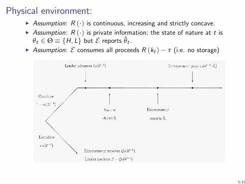
Physical environment:I Assumption: R (�) is continuous, increasing and strictly concave.
I Assumption: R (�) is private information; the state of nature at t isθt 2 Θ � fH, Lg but E reports θt .
I Assumption: E consumes all proceeds R (kt )� τ (i.e. no storage)
5/21
Physical environment:I Assumption: R (�) is continuous, increasing and strictly concave.I Assumption: R (�) is private information; the state of nature at t is
θt 2 Θ � fH, Lg but E reports θt .
I Assumption: E consumes all proceeds R (kt )� τ (i.e. no storage)
5/21
Physical environment:I Assumption: R (�) is continuous, increasing and strictly concave.I Assumption: R (�) is private information; the state of nature at t is
θt 2 Θ � fH, Lg but E reports θt .I Assumption: E consumes all proceeds R (kt )� τ (i.e. no storage)
5/21
Physical environment:
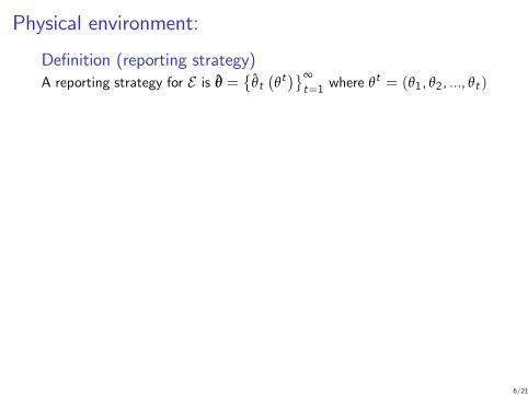
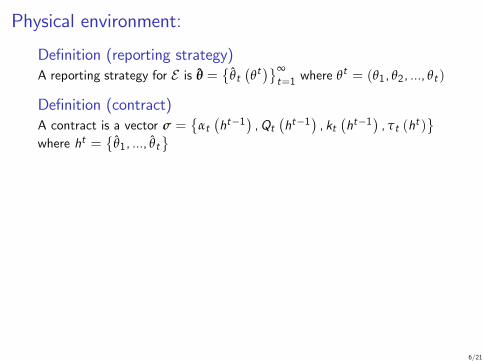
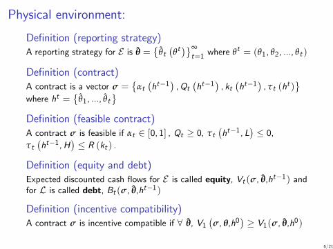
De�nition (reporting strategy)A reporting strategy for E is θ =
�θt�θt�∞t=1 where θt = (θ1, θ2, ..., θt )
De�nition (contract)A contract is a vector σ =
�αt�ht�1
�,Qt
�ht�1
�, kt
�ht�1
�, τt (ht )
where ht =
�θ1, ..., θt
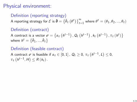
De�nition (feasible contract)A contract σ is feasible if αt 2 [0, 1] , Qt � 0, τt
�ht�1, L
�� 0,
τt�ht�1,H
�� R (kt ) .
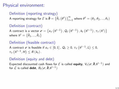
De�nition (equity and debt)Expected discounted cash �ows for E is called equity, Vt (σ, θ,ht�1) andfor L is called debt, Bt (σ, θ,ht�1)
De�nition (incentive compatibility)A contract σ is incentive compatible if 8 θ, V1
�σ, θ,h0
�� V1(σ, θ,h0)
6/21
Physical environment:
De�nition (reporting strategy)A reporting strategy for E is θ =
�θt�θt�∞t=1 where θt = (θ1, θ2, ..., θt )
De�nition (contract)A contract is a vector σ =
�αt�ht�1
�,Qt
�ht�1
�, kt
�ht�1
�, τt (ht )
where ht =
�θ1, ..., θt
De�nition (feasible contract)A contract σ is feasible if αt 2 [0, 1] , Qt � 0, τt
�ht�1, L
�� 0,
τt�ht�1,H
�� R (kt ) .
De�nition (equity and debt)Expected discounted cash �ows for E is called equity, Vt (σ, θ,ht�1) andfor L is called debt, Bt (σ, θ,ht�1)
De�nition (incentive compatibility)A contract σ is incentive compatible if 8 θ, V1
�σ, θ,h0
�� V1(σ, θ,h0)
6/21
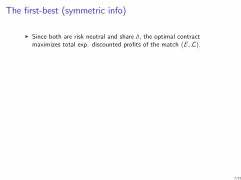
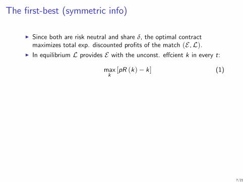
The �rst-best (symmetric info)
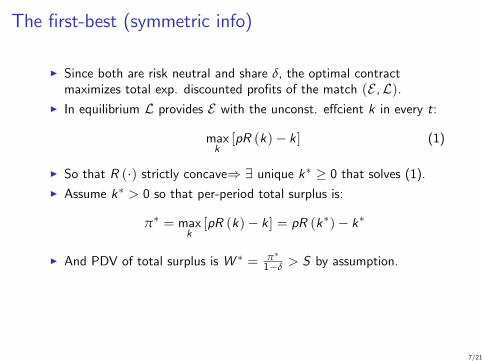
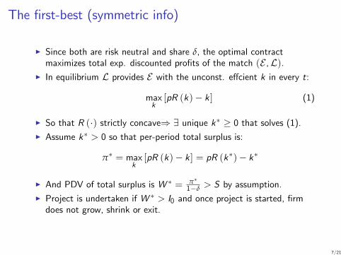
I Since both are risk neutral and share δ, the optimal contractmaximizes total exp. discounted pro�ts of the match (E ,L).
I In equilibrium L provides E with the unconst. e¤cient k in every t:
maxk[pR (k)� k ] (1)
I So that R (�) strictly concave) 9 unique k� � 0 that solves (1).I Assume k� > 0 so that per-period total surplus is:
π� = maxk[pR (k)� k ] = pR (k�)� k�
I And PDV of total surplus is W � = π�1�δ > S by assumption.
I Project is undertaken if W � > I0 and once project is started, �rmdoes not grow, shrink or exit.
7/21
The �rst-best (symmetric info)
I Since both are risk neutral and share δ, the optimal contractmaximizes total exp. discounted pro�ts of the match (E ,L).
I In equilibrium L provides E with the unconst. e¤cient k in every t:
maxk[pR (k)� k ] (1)
I So that R (�) strictly concave) 9 unique k� � 0 that solves (1).I Assume k� > 0 so that per-period total surplus is:
π� = maxk[pR (k)� k ] = pR (k�)� k�
I And PDV of total surplus is W � = π�1�δ > S by assumption.
I Project is undertaken if W � > I0 and once project is started, �rmdoes not grow, shrink or exit.
7/21

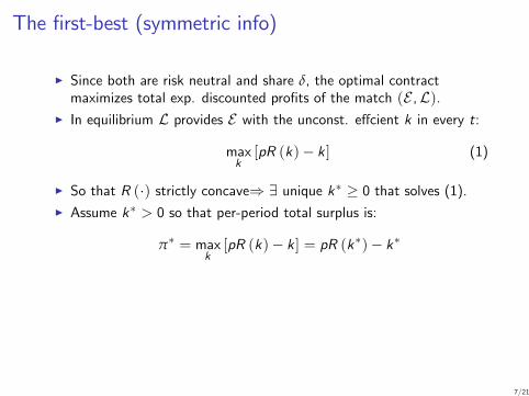
The �rst-best (symmetric info)
I Since both are risk neutral and share δ, the optimal contractmaximizes total exp. discounted pro�ts of the match (E ,L).
I In equilibrium L provides E with the unconst. e¤cient k in every t:
maxk[pR (k)� k ] (1)
I So that R (�) strictly concave) 9 unique k� � 0 that solves (1).
I Assume k� > 0 so that per-period total surplus is:
π� = maxk[pR (k)� k ] = pR (k�)� k�
I And PDV of total surplus is W � = π�1�δ > S by assumption.
I Project is undertaken if W � > I0 and once project is started, �rmdoes not grow, shrink or exit.
7/21
The �rst-best (symmetric info)
I Since both are risk neutral and share δ, the optimal contractmaximizes total exp. discounted pro�ts of the match (E ,L).
I In equilibrium L provides E with the unconst. e¤cient k in every t:
maxk[pR (k)� k ] (1)
I So that R (�) strictly concave) 9 unique k� � 0 that solves (1).I Assume k� > 0 so that per-period total surplus is:
π� = maxk[pR (k)� k ] = pR (k�)� k�
I And PDV of total surplus is W � = π�1�δ > S by assumption.
I Project is undertaken if W � > I0 and once project is started, �rmdoes not grow, shrink or exit.
7/21
Private information: the Pareto frontier
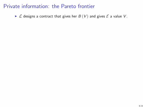
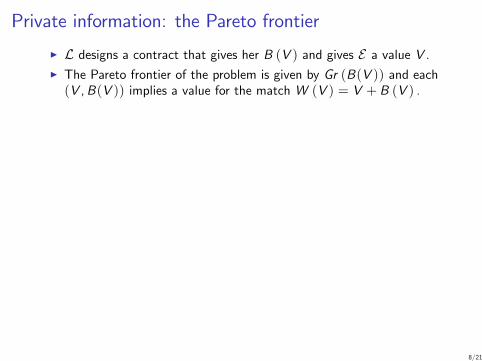
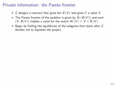
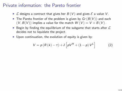
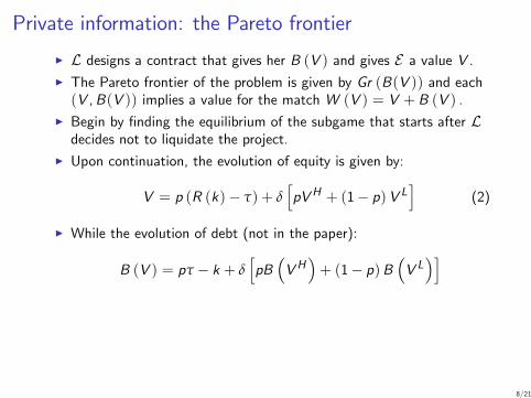
I L designs a contract that gives her B (V ) and gives E a value V .
I The Pareto frontier of the problem is given by Gr (B(V )) and each(V ,B(V )) implies a value for the match W (V ) = V + B (V ) .
I Begin by �nding the equilibrium of the subgame that starts after Ldecides not to liquidate the project.
I Upon continuation, the evolution of equity is given by:
V = p (R (k)� τ) + δhpVH + (1� p)V L
i(2)
I While the evolution of debt (not in the paper):
B (V ) = pτ � k + δhpB�VH
�+ (1� p)B
�V L�i
I The value of equity e¤ectively summarizes all the informationprovided by the history itself (Spear and Srivastava, 1987; Green,1987) so it�s the appropriate state variable in a recursive formulationof the repeated contracting problem.
8/21
Private information: the Pareto frontier
I L designs a contract that gives her B (V ) and gives E a value V .I The Pareto frontier of the problem is given by Gr (B(V )) and each(V ,B(V )) implies a value for the match W (V ) = V + B (V ) .
I Begin by �nding the equilibrium of the subgame that starts after Ldecides not to liquidate the project.
I Upon continuation, the evolution of equity is given by:
V = p (R (k)� τ) + δhpVH + (1� p)V L
i(2)
I While the evolution of debt (not in the paper):
B (V ) = pτ � k + δhpB�VH
�+ (1� p)B
�V L�i
I The value of equity e¤ectively summarizes all the informationprovided by the history itself (Spear and Srivastava, 1987; Green,1987) so it�s the appropriate state variable in a recursive formulationof the repeated contracting problem.
8/21
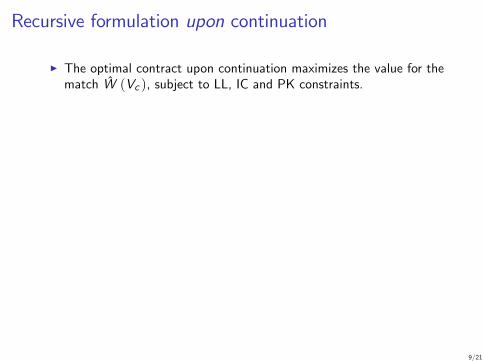
Recursive formulation upon continuation
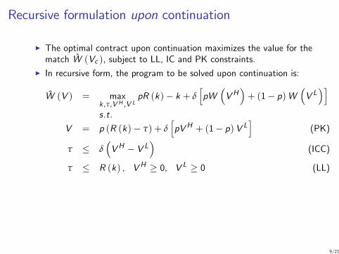
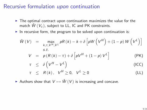
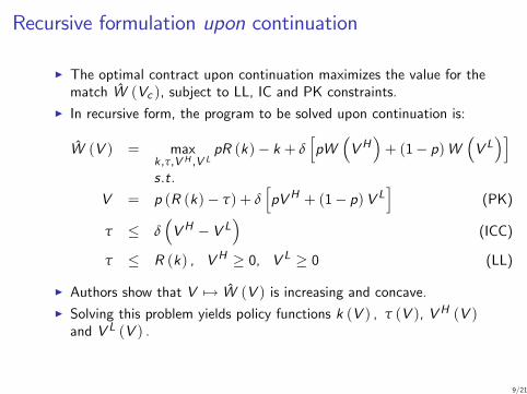
I The optimal contract upon continuation maximizes the value for thematch W (Vc ), subject to LL, IC and PK constraints.
I In recursive form, the program to be solved upon continuation is:
W (V ) = maxk ,τ,V H ,V L
pR (k)� k + δhpW
�VH
�+ (1� p)W
�V L�i
s.t.
V = p (R (k)� τ) + δhpVH + (1� p)V L
i(PK)
τ � δ�VH � V L
�(ICC)
τ � R (k) , VH � 0, V L � 0 (LL)
I Authors show that V 7! W (V ) is increasing and concave.I Solving this problem yields policy functions k (V ) , τ (V ), VH (V )and V L (V ) .
9/21
Recursive formulation upon continuation
I The optimal contract upon continuation maximizes the value for thematch W (Vc ), subject to LL, IC and PK constraints.
I In recursive form, the program to be solved upon continuation is:
W (V ) = maxk ,τ,V H ,V L
pR (k)� k + δhpW
�VH
�+ (1� p)W
�V L�i
s.t.
V = p (R (k)� τ) + δhpVH + (1� p)V L
i(PK)
τ � δ�VH � V L
�(ICC)
τ � R (k) , VH � 0, V L � 0 (LL)
I Authors show that V 7! W (V ) is increasing and concave.
I Solving this problem yields policy functions k (V ) , τ (V ), VH (V )and V L (V ) .
9/21
Recursive formulation upon continuation
I The optimal contract upon continuation maximizes the value for thematch W (Vc ), subject to LL, IC and PK constraints.
I In recursive form, the program to be solved upon continuation is:
W (V ) = maxk ,τ,V H ,V L
pR (k)� k + δhpW
�VH
�+ (1� p)W
�V L�i
s.t.
V = p (R (k)� τ) + δhpVH + (1� p)V L
i(PK)
τ � δ�VH � V L
�(ICC)
τ � R (k) , VH � 0, V L � 0 (LL)
I Authors show that V 7! W (V ) is increasing and concave.I Solving this problem yields policy functions k (V ) , τ (V ), VH (V )and V L (V ) .
9/21
Recursive formulation before liquidation decision
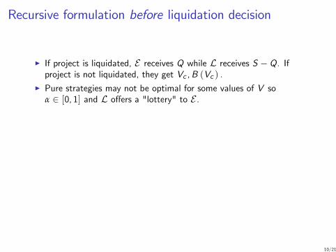
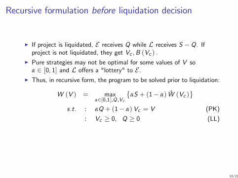
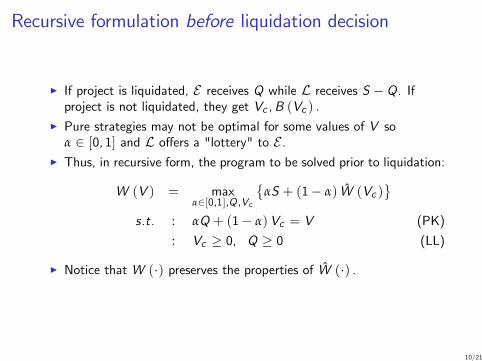
I If project is liquidated, E receives Q while L receives S �Q. Ifproject is not liquidated, they get Vc ,B (Vc ) .
I Pure strategies may not be optimal for some values of V soα 2 [0, 1] and L o¤ers a "lottery" to E .
I Thus, in recursive form, the program to be solved prior to liquidation:
W (V ) = maxα2[0,1],Q ,Vc
�αS + (1� α) W (Vc )
s.t. : αQ + (1� α)Vc = V (PK)
: Vc � 0, Q � 0 (LL)
I Notice that W (�) preserves the properties of W (�) .
10/21
Recursive formulation before liquidation decision
I If project is liquidated, E receives Q while L receives S �Q. Ifproject is not liquidated, they get Vc ,B (Vc ) .
I Pure strategies may not be optimal for some values of V soα 2 [0, 1] and L o¤ers a "lottery" to E .
I Thus, in recursive form, the program to be solved prior to liquidation:
W (V ) = maxα2[0,1],Q ,Vc
�αS + (1� α) W (Vc )
s.t. : αQ + (1� α)Vc = V (PK)
: Vc � 0, Q � 0 (LL)
I Notice that W (�) preserves the properties of W (�) .
10/21
Regions for V (Propositions 1 & 2)
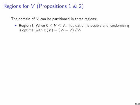
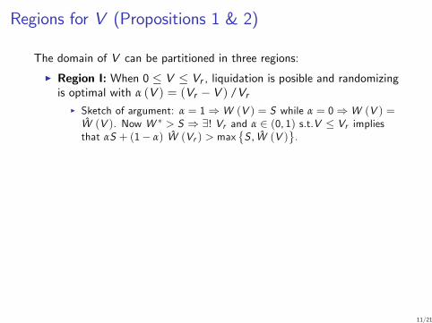
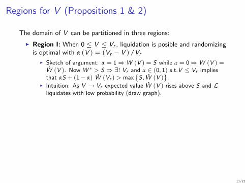
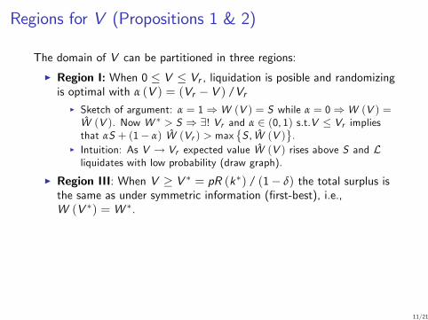
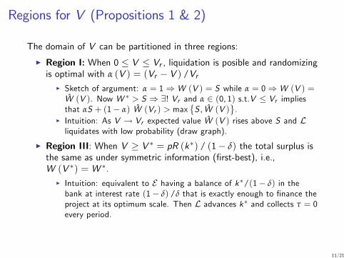
The domain of V can be partitioned in three regions:
I Region I: When 0 � V � Vr , liquidation is posible and randomizingis optimal with α (V ) = (Vr � V ) /Vr
I Sketch of argument: α = 1) W (V ) = S while α = 0) W (V ) =W (V ). Now W � > S ) 9! Vr and α 2 (0, 1) s.t.V � Vr impliesthat αS + (1� α) W (Vr ) > max
�S , W (V )
.
I Intuition: As V ! Vr expected value W (V ) rises above S and Lliquidates with low probability (draw graph).
I Region III: When V � V � = pR (k�) / (1� δ) the total surplus isthe same as under symmetric information (�rst-best), i.e.,W (V �) = W �.
I Intuition: equivalent to E having a balance of k�/(1� δ) in thebank at interest rate (1� δ) /δ that is exactly enough to �nance theproject at its optimum scale. Then L advances k� and collects τ = 0every period.
11/21
Regions for V (Propositions 1 & 2)
The domain of V can be partitioned in three regions:
I Region I: When 0 � V � Vr , liquidation is posible and randomizingis optimal with α (V ) = (Vr � V ) /Vr
I Sketch of argument: α = 1) W (V ) = S while α = 0) W (V ) =W (V ). Now W � > S ) 9! Vr and α 2 (0, 1) s.t.V � Vr impliesthat αS + (1� α) W (Vr ) > max
�S , W (V )
.
I Intuition: As V ! Vr expected value W (V ) rises above S and Lliquidates with low probability (draw graph).
I Region III: When V � V � = pR (k�) / (1� δ) the total surplus isthe same as under symmetric information (�rst-best), i.e.,W (V �) = W �.
I Intuition: equivalent to E having a balance of k�/(1� δ) in thebank at interest rate (1� δ) /δ that is exactly enough to �nance theproject at its optimum scale. Then L advances k� and collects τ = 0every period.
11/21
The borrowing constraint region (Propositions 1 & 2 cont.)
I Region II: When Vr � V < V �:
(a) There is no liquidation in current period and V 7! W (V ) is strictlyincreasing and,
(b) The optimal capital advancement policy is single-valued and s.t.k (V ) < k� (the �rms is debt-constrained)
I Sketch of argument: suppose that the optimal repayment policy forregion II was τ = R (k) implying that the ICC binds (see below theproofs for both of these results). Then:
R (k) = δ(VH � V L)
which implies that increasing k is only incentive compatible ifVH � V L also increases. But W (V ) concave implies that doing sois costly! (draw graph)
12/21
The borrowing constraint region (Propositions 1 & 2 cont.)
I Region II: When Vr � V < V �:(a) There is no liquidation in current period and V 7! W (V ) is strictly
increasing and,
(b) The optimal capital advancement policy is single-valued and s.t.k (V ) < k� (the �rms is debt-constrained)
I Sketch of argument: suppose that the optimal repayment policy forregion II was τ = R (k) implying that the ICC binds (see below theproofs for both of these results). Then:
R (k) = δ(VH � V L)
which implies that increasing k is only incentive compatible ifVH � V L also increases. But W (V ) concave implies that doing sois costly! (draw graph)
12/21
The borrowing constraint region (Propositions 1 & 2 cont.)
I Region II: When Vr � V < V �:(a) There is no liquidation in current period and V 7! W (V ) is strictly
increasing and,(b) The optimal capital advancement policy is single-valued and s.t.
k (V ) < k� (the �rms is debt-constrained)
I Sketch of argument: suppose that the optimal repayment policy forregion II was τ = R (k) implying that the ICC binds (see below theproofs for both of these results). Then:
R (k) = δ(VH � V L)
which implies that increasing k is only incentive compatible ifVH � V L also increases. But W (V ) concave implies that doing sois costly! (draw graph)
12/21

Optimal repayment policy (proposition 3)
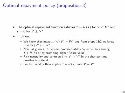
I The optimal repayment function satis�es τ = R (k) for V < V � andτ = 0 for V � V �.
I Intuition:
I We know that maxV 2V W (V ) = W � and from props 1&2 we knowthat W (V �) = W �.
I Now, at given t, L delivers promised utility Vt either by allowingτ < R (k) or by promising higher future value.
I Risk neutrality and common δ ) V ! V � in the shortest timepossible is optimal.
I Limited liability then implies τ = R (k) until V = V �
13/21
Optimal repayment policy (proposition 3)
I The optimal repayment function satis�es τ = R (k) for V < V � andτ = 0 for V � V �.
I Intuition:I We know that maxV 2V W (V ) = W � and from props 1&2 we knowthat W (V �) = W �.
I Now, at given t, L delivers promised utility Vt either by allowingτ < R (k) or by promising higher future value.
I Risk neutrality and common δ ) V ! V � in the shortest timepossible is optimal.
I Limited liability then implies τ = R (k) until V = V �
13/21
Evolution of equity when V < V �
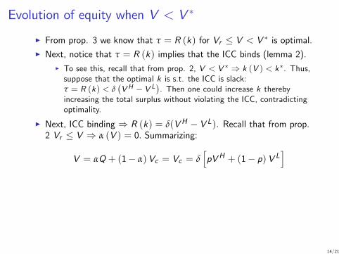
I From prop. 3 we know that τ = R (k) for Vr � V < V � is optimal.
I Next, notice that τ = R (k) implies that the ICC binds (lemma 2).
I To see this, recall that from prop. 2, V < V � ) k (V ) < k�. Thus,suppose that the optimal k is s.t. the ICC is slack:τ = R (k) < δ
�V H � V L
�. Then one could increase k thereby
increasing the total surplus without violating the ICC, contradictingoptimality.
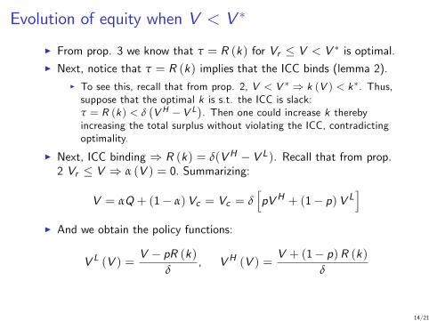
I Next, ICC binding ) R (k) = δ(VH � V L). Recall that from prop.2 Vr � V ) α (V ) = 0. Summarizing:
V = αQ + (1� α)Vc = Vc = δhpVH + (1� p)V L
iI And we obtain the policy functions:
V L (V ) =V � pR (k)
δ, VH (V ) =
V + (1� p)R (k)δ
14/21
Evolution of equity when V < V �
I From prop. 3 we know that τ = R (k) for Vr � V < V � is optimal.I Next, notice that τ = R (k) implies that the ICC binds (lemma 2).
I To see this, recall that from prop. 2, V < V � ) k (V ) < k�. Thus,suppose that the optimal k is s.t. the ICC is slack:τ = R (k) < δ
�V H � V L
�. Then one could increase k thereby
increasing the total surplus without violating the ICC, contradictingoptimality.
I Next, ICC binding ) R (k) = δ(VH � V L). Recall that from prop.2 Vr � V ) α (V ) = 0. Summarizing:
V = αQ + (1� α)Vc = Vc = δhpVH + (1� p)V L
i
I And we obtain the policy functions:
V L (V ) =V � pR (k)
δ, VH (V ) =
V + (1� p)R (k)δ
14/21
Evolution of equity when V < V �
I From prop. 3 we know that τ = R (k) for Vr � V < V � is optimal.I Next, notice that τ = R (k) implies that the ICC binds (lemma 2).
I To see this, recall that from prop. 2, V < V � ) k (V ) < k�. Thus,suppose that the optimal k is s.t. the ICC is slack:τ = R (k) < δ
�V H � V L
�. Then one could increase k thereby
increasing the total surplus without violating the ICC, contradictingoptimality.
I Next, ICC binding ) R (k) = δ(VH � V L). Recall that from prop.2 Vr � V ) α (V ) = 0. Summarizing:
V = αQ + (1� α)Vc = Vc = δhpVH + (1� p)V L
iI And we obtain the policy functions:
V L (V ) =V � pR (k)
δ, VH (V ) =
V + (1� p)R (k)δ
14/21
Evolution of equity when V < V �
I The authors show that V L (V ) ,VH (V ) are nondecreasing.
I Moreover, starting from any equity value V0 2 [Vr ,V �) after a �nitesequence of good shocks V0 ! V �.
I Likewise, after a �nite sequence of bad shocks V0 ! Vr or below,triggering randomized liquidation.
I There is an asymmetry between change in equity following good andbad shocks: if p, δ large ) V � V L > VH � V
15/21

Evolution of equity when V < V �
I The authors show that V L (V ) ,VH (V ) are nondecreasing.I Moreover, starting from any equity value V0 2 [Vr ,V �) after a �nitesequence of good shocks V0 ! V �.
I Likewise, after a �nite sequence of bad shocks V0 ! Vr or below,triggering randomized liquidation.
I There is an asymmetry between change in equity following good andbad shocks: if p, δ large ) V � V L > VH � V
15/21

Dynamics of equity
16/21
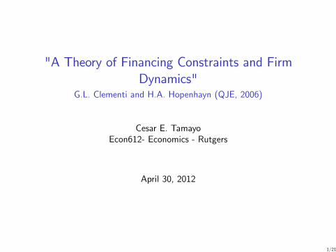
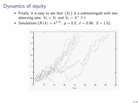
Dynamics of equityI Finally, it is easy to see that fVtg is a submartingale with twoabsorving sets: Vt < Vr and Vt > V � 8 t
I Simulations (R (k) = k2/5, p = 0.5, δ = 0.99, S = 1.5):
17/21
Dynamics of equityI Finally, it is easy to see that fVtg is a submartingale with twoabsorving sets: Vt < Vr and Vt > V � 8 t
I Simulations (R (k) = k2/5, p = 0.5, δ = 0.99, S = 1.5):
17/21
Optimal k advancement policy
I We�ve seen that V0 2 [Vr ,V �)) k (V ) < k� (the �rms isdebt-constrained).
I Now, it is di¢ cult to characterize V 7! k (V ) in general (it isnonmonotonic).
I However, simulations show that conditional on success, capital growsat a positve rate, i.e. k(VH )/k (V ) > 1 while k(V L)/k (V ) < 1.
I This contributes to the "cash-�ow coe¢ cient" debate; if Tobin�s q isa su¢ cient statistic for investment, then cash �ows should notmatter.
I But if the optimal contract of this model was the DGP:
1. Cash �ows will matter for investment, k (V ) < k�
2. Cash �ows will matter more, the more constrained is the �rm.
18/21

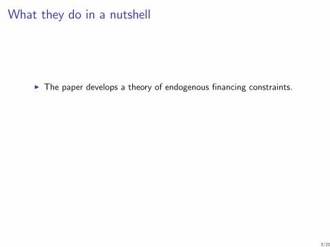
Firm growth and survival
I Firm size is captured by k
I Starting frm the same V0 2 [Vr ,V �) simulate many di¤erent shockpaths.
I As seen before, �rms eventually either exit or reach theunconstrained optimum size.
I Since k < k� w/e Vt < V � surviving �rms grow with age; size andage are positively correlated in accordance with empirical evidence.
I Mean and variance of equity growth decrease sistematically.I Conditional probability of survival increases with V . Given that Vincreases over time (for surviving �rms), survival rates are positivelycorrelated with age and size.
I The advantage of this model is that requires little structure on thestochastic process driving �rm productivity; a simple i.i.d. process isenough to generate the rich dynamics described above.
19/21
Firm growth and survival
I Firm size is captured by kI Starting frm the same V0 2 [Vr ,V �) simulate many di¤erent shockpaths.
I As seen before, �rms eventually either exit or reach theunconstrained optimum size.
I Since k < k� w/e Vt < V � surviving �rms grow with age; size andage are positively correlated in accordance with empirical evidence.
I Mean and variance of equity growth decrease sistematically.
I Conditional probability of survival increases with V . Given that Vincreases over time (for surviving �rms), survival rates are positivelycorrelated with age and size.
I The advantage of this model is that requires little structure on thestochastic process driving �rm productivity; a simple i.i.d. process isenough to generate the rich dynamics described above.
19/21
Firm growth and survival
I Firm size is captured by kI Starting frm the same V0 2 [Vr ,V �) simulate many di¤erent shockpaths.
I As seen before, �rms eventually either exit or reach theunconstrained optimum size.
I Since k < k� w/e Vt < V � surviving �rms grow with age; size andage are positively correlated in accordance with empirical evidence.
I Mean and variance of equity growth decrease sistematically.I Conditional probability of survival increases with V . Given that Vincreases over time (for surviving �rms), survival rates are positivelycorrelated with age and size.
I The advantage of this model is that requires little structure on thestochastic process driving �rm productivity; a simple i.i.d. process isenough to generate the rich dynamics described above.
19/21
Firm growth and survival
I Firm size is captured by kI Starting frm the same V0 2 [Vr ,V �) simulate many di¤erent shockpaths.
I As seen before, �rms eventually either exit or reach theunconstrained optimum size.
I Since k < k� w/e Vt < V � surviving �rms grow with age; size andage are positively correlated in accordance with empirical evidence.
I Mean and variance of equity growth decrease sistematically.I Conditional probability of survival increases with V . Given that Vincreases over time (for surviving �rms), survival rates are positivelycorrelated with age and size.
I The advantage of this model is that requires little structure on thestochastic process driving �rm productivity; a simple i.i.d. process isenough to generate the rich dynamics described above.
19/21

Firm growth and survival
20/21

Beyond �rm dynamics (not presented here)
I The authors show that the optimal (long term) contract can bereplicated by a sequence of one-period contracts i¤ it isrenegotiation-proof.
I The contract is renegotiation-proof i¤ collateral S is greater thanthe maximum sustainable debt.
I Risk aversion?I No capital accumulation is WLOG?I General equilibrium?
21/21
Beyond �rm dynamics (not presented here)
I The authors show that the optimal (long term) contract can bereplicated by a sequence of one-period contracts i¤ it isrenegotiation-proof.
I The contract is renegotiation-proof i¤ collateral S is greater thanthe maximum sustainable debt.
I Risk aversion?
I No capital accumulation is WLOG?I General equilibrium?
21/21

Beyond �rm dynamics (not presented here)
I The authors show that the optimal (long term) contract can bereplicated by a sequence of one-period contracts i¤ it isrenegotiation-proof.
I The contract is renegotiation-proof i¤ collateral S is greater thanthe maximum sustainable debt.
I Risk aversion?I No capital accumulation is WLOG?
I General equilibrium?
21/21
Beyond �rm dynamics (not presented here)
I The authors show that the optimal (long term) contract can bereplicated by a sequence of one-period contracts i¤ it isrenegotiation-proof.
I The contract is renegotiation-proof i¤ collateral S is greater thanthe maximum sustainable debt.
I Risk aversion?I No capital accumulation is WLOG?I General equilibrium?
21/21