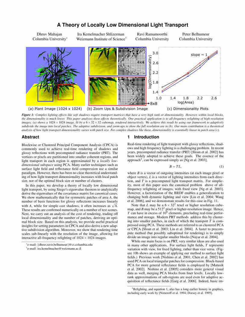
A Theory of Locally Low Dimensional Light Transport

Dhruv MahajanColumbia University∗

Ira Kemelmacher ShlizermanWeizmann Institute of Science†

Ravi RamamoorthiColumbia University

Peter BelhumeurColumbia University

4x4

8x8

1.4

1.8

2.2

2.6

3.0

1.0 1.4 1.8 2.2 2.6log(Area)

log(D

imen

sional

ity)

slope ~ 1

(a) Plant Image (1024 x 1024) (b) Zoom Ups & Subdivision Image (c) Dimensionality Plots

Figure 1: Complex lighting effects like soft shadows require transport matrices that have a very high rank or dimensionality. However, within local blocks,the dimensionality is much lower. This paper analyzes these effects theoretically. One practical application is to all-frequency relighting of high-resolutionimages; (a) shows a 1024× 1024 image, lit by a 6× 32× 32 cubemap, rendered interactively. We achieve this result by using our framework to adaptivelysubdivide the image into local patches. The adaptive subdivision, and zoom-ups to show the full resolution are in (b). Our main contribution is a theoreticalanalysis of how light transport dimensionality varies with patch size. For complex shadows like these, dimensionality is essentially linear in patch area (c).

Abstract

Blockwise or Clustered Principal Component Analysis (CPCA) iscommonly used to achieve real-time rendering of shadows andglossy reflections with precomputed radiance transfer (PRT). Thevertices or pixels are partitioned into smaller coherent regions, andlight transport in each region is approximated by a locally low-dimensional subspace using PCA. Many earlier techniques such assurface light field and reflectance field compression use a similarparadigm. However, there has been no clear theoretical understand-ing of how light transport dimensionality increases with local patchsize, nor of the optimal block size or number of clusters.

In this paper, we develop a theory of locally low dimensionallight transport, by using Szego’s eigenvalue theorem to analyticallyderive the eigenvalues of the covariance matrix for canonical cases.We show mathematically that for symmetric patches of area A, thenumber of basis functions for glossy reflections increases linearlywith A, while for simple cast shadows, it often increases as

√A.

These results are confirmed numerically on a number of test scenes.Next, we carry out an analysis of the cost of rendering, trading offlocal dimensionality and the number of patches, deriving an opti-mal block size. Based on this analysis, we provide useful practicalinsights for setting parameters in CPCA and also derive a new adap-tive subdivision algorithm. Moreover, we show that rendering timescales sub-linearly with the resolution of the image, allowing forinteractive all-frequency relighting of 1024×1024 images.

∗e-mail: dhruv,ravir,belhumeur@cs.columbia.edu†e-mail: ira.kemelmacher@weizmann.ac.il

1 Introduction

Real-time rendering of light transport with glossy reflections, shad-ows and high frequency lighting is a challenging problem. In recentyears, precomputed radiance transfer (PRT) [Sloan et al. 2002] hasbeen widely adopted to achieve these goals. The essence of theapproach1, can be expressed simply as [Ng et al. 2003],

B = T L, (1)

where B is a vector of outgoing intensities (at each image pixel orobject vertex), L is a vector of lighting intensities from each direc-tion, and T is a precomputed light transport matrix. For simplic-ity, most of this paper uses the canonical problem above of all-frequency relighting of images, with fixed view [Ng et al. 2003].However, a factorization of the BRDF enables a generalization tochanging both dynamic lighting and view [Liu et al. 2004; Wanget al. 2006], and we demonstrate results for this case in Fig. 11.

Note that L may be a 6× 322 texel or higher resolution cube-map, and B may be a 5122 pixel or higher-resolution image. Hence,T can have in excess of 109 elements, precluding real-time perfor-mance and storage. Modern PRT methods address this by cluster-ing into smaller patches, in each of which the transport T is com-pressed using PCA. These methods are referred to as clustered PCAor CPCA [Sloan et al. 2003; Liu et al. 2004]. A faster to precom-pute method (but possibly suboptimal for rendering) is to simplydivide an image into regular smaller blocks [Nayar et al. 2004].

While our main focus is on PRT, very similar ideas are also usedin many other applications. For surface light fields, T representsvariation with view, for fixed lighting, rather than vice versa. (Fig-ure 10b shows an example of applying our method to surface lightfields.) Previous work [Nishino et al. 2001; Chen et al. 2002] hasused PCA on local triangular patches for compression. Block-basedPCA for more general reflectance fields is employed by [Matusiket al. 2002]. Nishino et al. [2005] considers more general visualdata as well, merging PCA blocks from finer levels. Locally low-rank approximations of sub-regions are used even for adaptive ac-quisition of reflectance fields [Garg et al. 2006]. Indeed, basic im-

1Relighting, and equation 1, also has a long earlier history in graphics,including early work by [Nimeroff et al. 1994; Dorsey et al. 1995].

1 2 4 8 16 320

20

40

80

60

100

120

Cost

per

Pix

el

Patch Size(Square Side)

DimensionalityOverhead CostTotal Cost

Optimal Cost

Low

High

High

Low

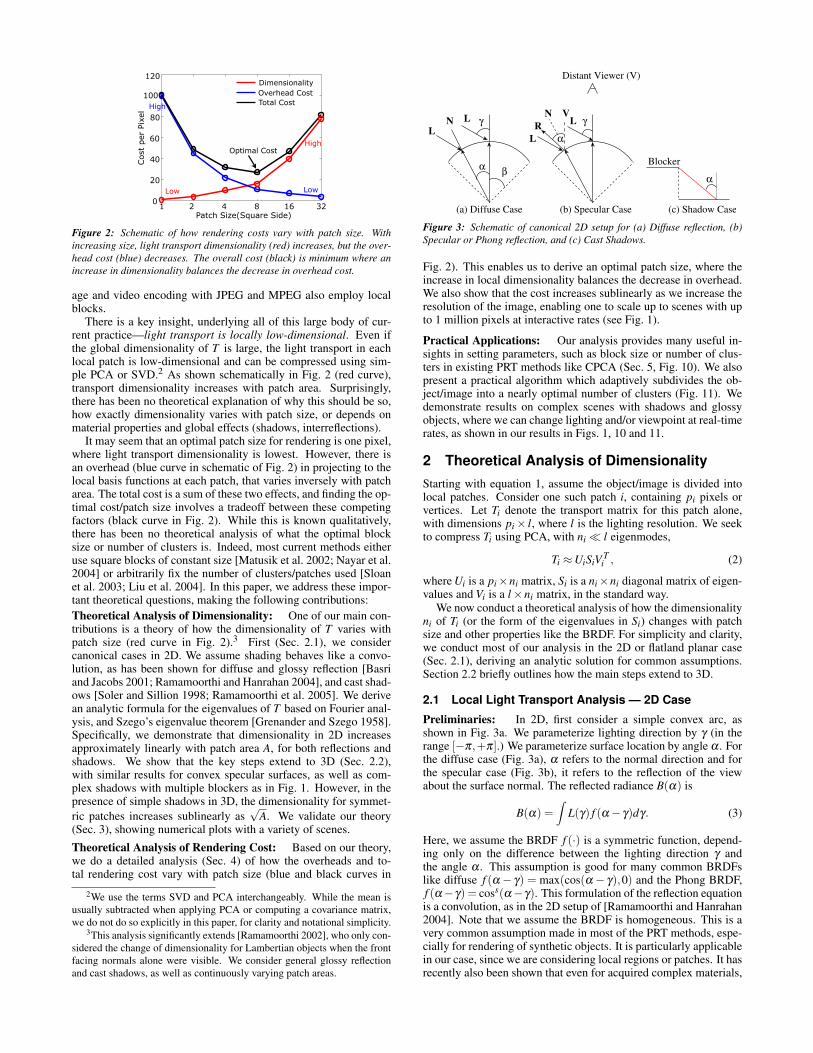
Figure 2: Schematic of how rendering costs vary with patch size. Withincreasing size, light transport dimensionality (red) increases, but the over-head cost (blue) decreases. The overall cost (black) is minimum where anincrease in dimensionality balances the decrease in overhead cost.

age and video encoding with JPEG and MPEG also employ localblocks.

There is a key insight, underlying all of this large body of cur-rent practice—light transport is locally low-dimensional. Even ifthe global dimensionality of T is large, the light transport in eachlocal patch is low-dimensional and can be compressed using sim-ple PCA or SVD.2 As shown schematically in Fig. 2 (red curve),transport dimensionality increases with patch area. Surprisingly,there has been no theoretical explanation of why this should be so,how exactly dimensionality varies with patch size, or depends onmaterial properties and global effects (shadows, interreflections).

It may seem that an optimal patch size for rendering is one pixel,where light transport dimensionality is lowest. However, there isan overhead (blue curve in schematic of Fig. 2) in projecting to thelocal basis functions at each patch, that varies inversely with patcharea. The total cost is a sum of these two effects, and finding the op-timal cost/patch size involves a tradeoff between these competingfactors (black curve in Fig. 2). While this is known qualitatively,there has been no theoretical analysis of what the optimal blocksize or number of clusters is. Indeed, most current methods eitheruse square blocks of constant size [Matusik et al. 2002; Nayar et al.2004] or arbitrarily fix the number of clusters/patches used [Sloanet al. 2003; Liu et al. 2004]. In this paper, we address these impor-tant theoretical questions, making the following contributions:Theoretical Analysis of Dimensionality: One of our main con-tributions is a theory of how the dimensionality of T varies withpatch size (red curve in Fig. 2).3 First (Sec. 2.1), we considercanonical cases in 2D. We assume shading behaves like a convo-lution, as has been shown for diffuse and glossy reflection [Basriand Jacobs 2001; Ramamoorthi and Hanrahan 2004], and cast shad-ows [Soler and Sillion 1998; Ramamoorthi et al. 2005]. We derivean analytic formula for the eigenvalues of T based on Fourier anal-ysis, and Szego’s eigenvalue theorem [Grenander and Szego 1958].Specifically, we demonstrate that dimensionality in 2D increasesapproximately linearly with patch area A, for both reflections andshadows. We show that the key steps extend to 3D (Sec. 2.2),with similar results for convex specular surfaces, as well as com-plex shadows with multiple blockers as in Fig. 1. However, in thepresence of simple shadows in 3D, the dimensionality for symmet-ric patches increases sublinearly as

√A. We validate our theory

(Sec. 3), showing numerical plots with a variety of scenes.

Theoretical Analysis of Rendering Cost: Based on our theory,we do a detailed analysis (Sec. 4) of how the overheads and to-tal rendering cost vary with patch size (blue and black curves in

2We use the terms SVD and PCA interchangeably. While the mean isusually subtracted when applying PCA or computing a covariance matrix,we do not do so explicitly in this paper, for clarity and notational simplicity.

3This analysis significantly extends [Ramamoorthi 2002], who only con-sidered the change of dimensionality for Lambertian objects when the frontfacing normals alone were visible. We consider general glossy reflectionand cast shadows, as well as continuously varying patch areas.

α

(c) Shadow Case

Blocker

Rα

N V

(b) Specular Case

Distant Viewer (V)

NL

βα

(a) Diffuse Case

LL

L

γγ

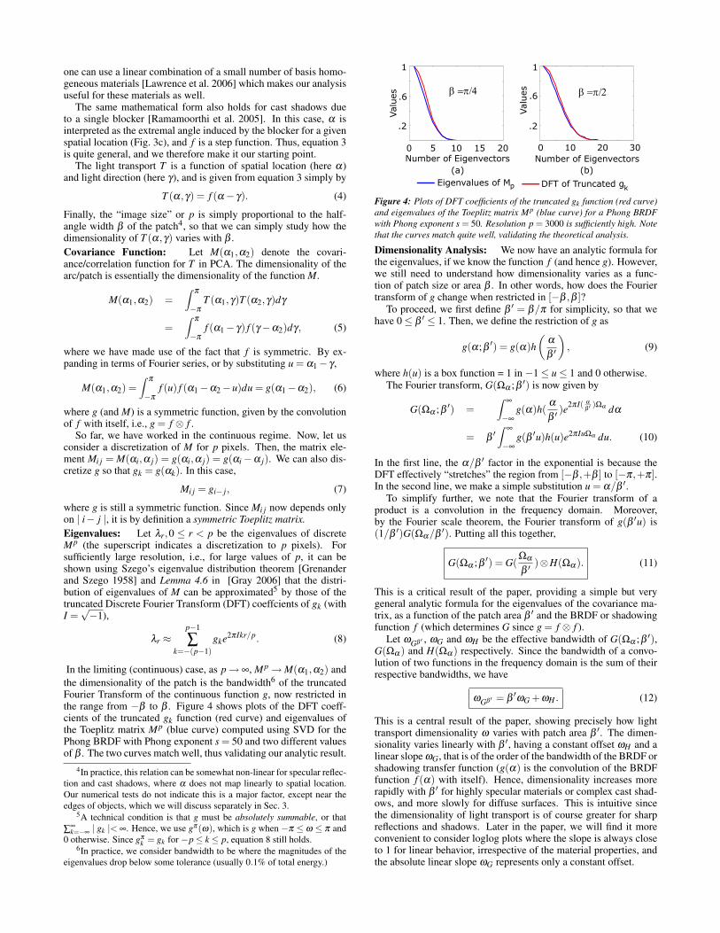
Figure 3: Schematic of canonical 2D setup for (a) Diffuse reflection, (b)Specular or Phong reflection, and (c) Cast Shadows.

Fig. 2). This enables us to derive an optimal patch size, where theincrease in local dimensionality balances the decrease in overhead.We also show that the cost increases sublinearly as we increase theresolution of the image, enabling one to scale up to scenes with upto 1 million pixels at interactive rates (see Fig. 1).

Practical Applications: Our analysis provides many useful in-sights in setting parameters, such as block size or number of clus-ters in existing PRT methods like CPCA (Sec. 5, Fig. 10). We alsopresent a practical algorithm which adaptively subdivides the ob-ject/image into a nearly optimal number of clusters (Fig. 11). Wedemonstrate results on complex scenes with shadows and glossyobjects, where we can change lighting and/or viewpoint at real-timerates, as shown in our results in Figs. 1, 10 and 11.

2 Theoretical Analysis of DimensionalityStarting with equation 1, assume the object/image is divided intolocal patches. Consider one such patch i, containing pi pixels orvertices. Let Ti denote the transport matrix for this patch alone,with dimensions pi× l, where l is the lighting resolution. We seekto compress Ti using PCA, with ni l eigenmodes,

Ti ≈UiSiV Ti , (2)

where Ui is a pi×ni matrix, Si is a ni×ni diagonal matrix of eigen-values and Vi is a l×ni matrix, in the standard way.

We now conduct a theoretical analysis of how the dimensionalityni of Ti (or the form of the eigenvalues in Si) changes with patchsize and other properties like the BRDF. For simplicity and clarity,we conduct most of our analysis in the 2D or flatland planar case(Sec. 2.1), deriving an analytic solution for common assumptions.Section 2.2 briefly outlines how the main steps extend to 3D.

2.1 Local Light Transport Analysis — 2D Case

Preliminaries: In 2D, first consider a simple convex arc, asshown in Fig. 3a. We parameterize lighting direction by γ (in therange [−π,+π].) We parameterize surface location by angle α . Forthe diffuse case (Fig. 3a), α refers to the normal direction and forthe specular case (Fig. 3b), it refers to the reflection of the viewabout the surface normal. The reflected radiance B(α) is

B(α) =∫

L(γ) f (α− γ)dγ. (3)

Here, we assume the BRDF f (·) is a symmetric function, depend-ing only on the difference between the lighting direction γ andthe angle α . This assumption is good for many common BRDFslike diffuse f (α − γ) = max(cos(α − γ),0) and the Phong BRDF,f (α−γ) = coss(α−γ). This formulation of the reflection equationis a convolution, as in the 2D setup of [Ramamoorthi and Hanrahan2004]. Note that we assume the BRDF is homogeneous. This is avery common assumption made in most of the PRT methods, espe-cially for rendering of synthetic objects. It is particularly applicablein our case, since we are considering local regions or patches. It hasrecently also been shown that even for acquired complex materials,

one can use a linear combination of a small number of basis homo-geneous materials [Lawrence et al. 2006] which makes our analysisuseful for these materials as well.

The same mathematical form also holds for cast shadows dueto a single blocker [Ramamoorthi et al. 2005]. In this case, α isinterpreted as the extremal angle induced by the blocker for a givenspatial location (Fig. 3c), and f is a step function. Thus, equation 3is quite general, and we therefore make it our starting point.

The light transport T is a function of spatial location (here α)and light direction (here γ), and is given from equation 3 simply by

T (α,γ) = f (α− γ). (4)

Finally, the “image size” or p is simply proportional to the half-angle width β of the patch4, so that we can simply study how thedimensionality of T (α,γ) varies with β .Covariance Function: Let M(α1,α2) denote the covari-ance/correlation function for T in PCA. The dimensionality of thearc/patch is essentially the dimensionality of the function M.

M(α1,α2) =∫

π

−π

T (α1,γ)T (α2,γ)dγ

=∫

π

−π

f (α1− γ) f (γ−α2)dγ, (5)

where we have made use of the fact that f is symmetric. By ex-panding in terms of Fourier series, or by substituting u = α1− γ ,

M(α1,α2) =∫

π

−π

f (u) f (α1−α2−u)du = g(α1−α2), (6)

where g (and M) is a symmetric function, given by the convolutionof f with itself, i.e., g = f ⊗ f .

So far, we have worked in the continuous regime. Now, let usconsider a discretization of M for p pixels. Then, the matrix ele-ment Mi j = M(αi,α j) = g(αi,α j) = g(αi−α j). We can also dis-cretize g so that gk = g(αk). In this case,

Mi j = gi− j, (7)

where g is still a symmetric function. Since Mi j now depends onlyon | i− j |, it is by definition a symmetric Toeplitz matrix.Eigenvalues: Let λr,0 ≤ r < p be the eigenvalues of discreteMp (the superscript indicates a discretization to p pixels). Forsufficiently large resolution, i.e., for large values of p, it can beshown using Szego’s eigenvalue distribution theorem [Grenanderand Szego 1958] and Lemma 4.6 in [Gray 2006] that the distri-bution of eigenvalues of M can be approximated5 by those of thetruncated Discrete Fourier Transform (DFT) coeffcients of gk (withI =

√−1),

λr ≈p−1

∑k=−(p−1)

gke2πIkr/p. (8)

In the limiting (continuous) case, as p→ ∞, Mp →M(α1,α2) andthe dimensionality of the patch is the bandwidth6 of the truncatedFourier Transform of the continuous function g, now restricted inthe range from −β to β . Figure 4 shows plots of the DFT coeff-cients of the truncated gk function (red curve) and eigenvalues ofthe Toeplitz matrix Mp (blue curve) computed using SVD for thePhong BRDF with Phong exponent s = 50 and two different valuesof β . The two curves match well, thus validating our analytic result.

4In practice, this relation can be somewhat non-linear for specular reflec-tion and cast shadows, where α does not map linearly to spatial location.Our numerical tests do not indicate this is a major factor, except near theedges of objects, which we will discuss separately in Sec. 3.

5A technical condition is that g must be absolutely summable, or that∑

∞k=−∞

| gk |< ∞. Hence, we use gπ (ω), which is g when −π ≤ ω ≤ π and0 otherwise. Since gπ

k = gk for −p≤ k ≤ p, equation 8 still holds.6In practice, we consider bandwidth to be where the magnitudes of the

eigenvalues drop below some tolerance (usually 0.1% of total energy.)

0 5 10 15 20 0 10 20 30

.2

.6

1

.2

.6

1

Val

ues

Val

ues

Number of Eigenvectors

Eigenvalues of Mp DFT of Truncated gk

Number of Eigenvectors

β =π/4 β =π/2

(a) (b)

Figure 4: Plots of DFT coefficients of the truncated gk function (red curve)and eigenvalues of the Toeplitz matrix Mp (blue curve) for a Phong BRDFwith Phong exponent s = 50. Resolution p = 3000 is sufficiently high. Notethat the curves match quite well, validating the theoretical analysis.

Dimensionality Analysis: We now have an analytic formula forthe eigenvalues, if we know the function f (and hence g). However,we still need to understand how dimensionality varies as a func-tion of patch size or area β . In other words, how does the Fouriertransform of g change when restricted in [−β ,β ]?

To proceed, we first define β ′ = β/π for simplicity, so that wehave 0≤ β ′ ≤ 1. Then, we define the restriction of g as

g(α;β′) = g(α)h

(α

β ′

), (9)

where h(u) is a box function = 1 in −1≤ u≤ 1 and 0 otherwise.The Fourier transform, G(Ωα ;β ′) is now given by

G(Ωα ;β′) =

∫∞

−∞

g(α)h(α

β ′)e2πI( α

β ′ )Ωα dα

= β′∫

∞

−∞

g(β ′u)h(u)e2πIuΩα du. (10)

In the first line, the α/β ′ factor in the exponential is because theDFT effectively “stretches” the region from [−β ,+β ] to [−π,+π].In the second line, we make a simple substitution u = α/β ′.

To simplify further, we note that the Fourier transform of aproduct is a convolution in the frequency domain. Moreover,by the Fourier scale theorem, the Fourier transform of g(β ′u) is(1/β ′)G(Ωα/β ′). Putting all this together,

G(Ωα ;β′) = G(

Ωα

β ′)⊗H(Ωα ). (11)

This is a critical result of the paper, providing a simple but verygeneral analytic formula for the eigenvalues of the covariance ma-trix, as a function of the patch area β ′ and the BRDF or shadowingfunction f (which determines G since g = f ⊗ f ).

Let ωGβ ′ , ωG and ωH be the effective bandwidth of G(Ωα ;β ′),G(Ωα ) and H(Ωα ) respectively. Since the bandwidth of a convo-lution of two functions in the frequency domain is the sum of theirrespective bandwidths, we have

ωGβ ′ = β′ωG +ωH . (12)

This is a central result of the paper, showing precisely how lighttransport dimensionality ω varies with patch area β ′. The dimen-sionality varies linearly with β ′, having a constant offset ωH and alinear slope ωG, that is of the order of the bandwidth of the BRDF orshadowing transfer function (g(α) is the convolution of the BRDFfunction f (α) with itself). Hence, dimensionality increases morerapidly with β ′ for highly specular materials or complex cast shad-ows, and more slowly for diffuse surfaces. This is intuitive sincethe dimensionality of light transport is of course greater for sharpreflections and shadows. Later in the paper, we will find it moreconvenient to consider loglog plots where the slope is always closeto 1 for linear behavior, irrespective of the material properties, andthe absolute linear slope ωG represents only a constant offset.

1.5

2.5

3.5

-3 -2 -1 0 1 log(β)

log(d

imen

sional

ity)

-3 -2 -1 0 1 log(β)

2

4

6s = 50s = 100

step blockerconcave arclo

g(d

imen

sional

ity)

(a) Convex arc (b) Shadow Case

linear region slope = 1

slope = 1

slope = 1

2.0

3.0

1.0

3

5

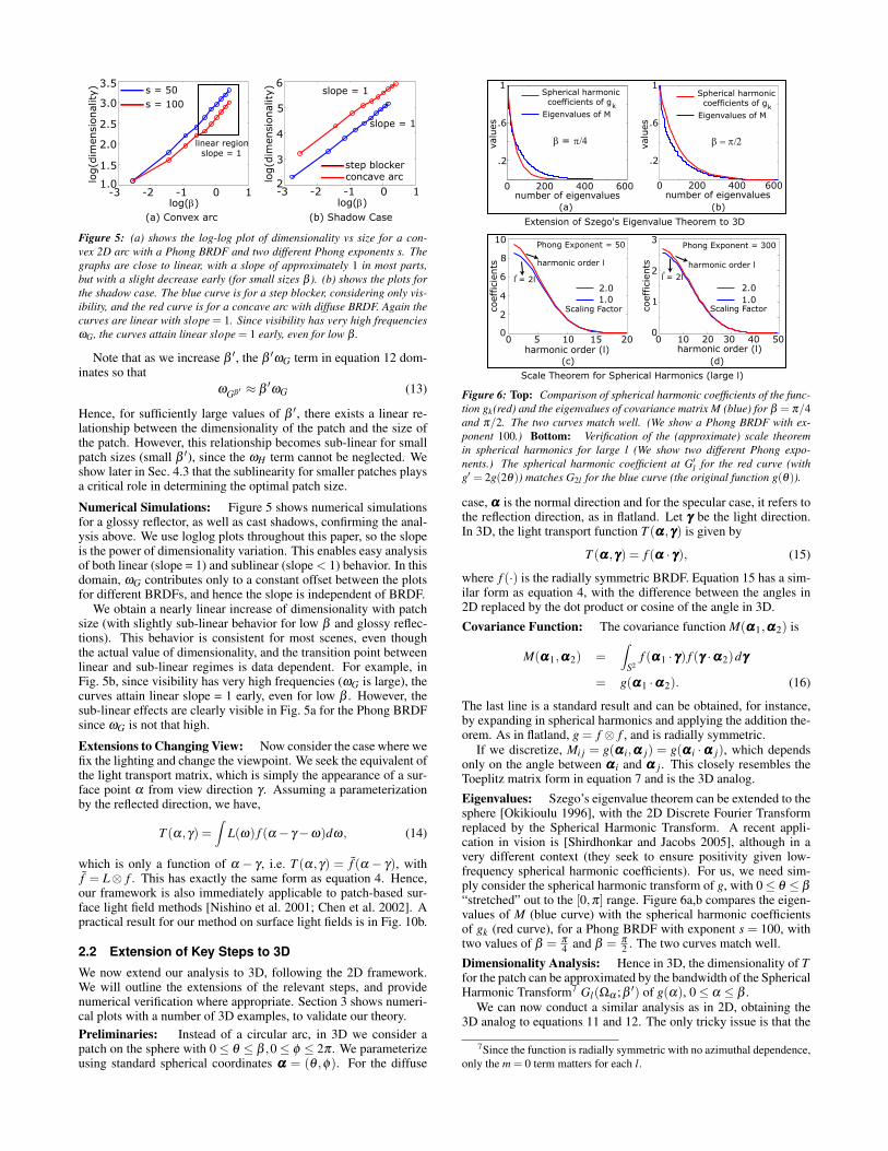
Figure 5: (a) shows the log-log plot of dimensionality vs size for a con-vex 2D arc with a Phong BRDF and two different Phong exponents s. Thegraphs are close to linear, with a slope of approximately 1 in most parts,but with a slight decrease early (for small sizes β ). (b) shows the plots forthe shadow case. The blue curve is for a step blocker, considering only vis-ibility, and the red curve is for a concave arc with diffuse BRDF. Again thecurves are linear with slope = 1. Since visibility has very high frequenciesωG, the curves attain linear slope = 1 early, even for low β .

Note that as we increase β ′, the β ′ωG term in equation 12 dom-inates so that

ωGβ ′ ≈ β′ωG (13)

Hence, for sufficiently large values of β ′, there exists a linear re-lationship between the dimensionality of the patch and the size ofthe patch. However, this relationship becomes sub-linear for smallpatch sizes (small β ′), since the ωH term cannot be neglected. Weshow later in Sec. 4.3 that the sublinearity for smaller patches playsa critical role in determining the optimal patch size.

Numerical Simulations: Figure 5 shows numerical simulationsfor a glossy reflector, as well as cast shadows, confirming the anal-ysis above. We use loglog plots throughout this paper, so the slopeis the power of dimensionality variation. This enables easy analysisof both linear (slope = 1) and sublinear (slope < 1) behavior. In thisdomain, ωG contributes only to a constant offset between the plotsfor different BRDFs, and hence the slope is independent of BRDF.

We obtain a nearly linear increase of dimensionality with patchsize (with slightly sub-linear behavior for low β and glossy reflec-tions). This behavior is consistent for most scenes, even thoughthe actual value of dimensionality, and the transition point betweenlinear and sub-linear regimes is data dependent. For example, inFig. 5b, since visibility has very high frequencies (ωG is large), thecurves attain linear slope = 1 early, even for low β . However, thesub-linear effects are clearly visible in Fig. 5a for the Phong BRDFsince ωG is not that high.

Extensions to Changing View: Now consider the case where wefix the lighting and change the viewpoint. We seek the equivalent ofthe light transport matrix, which is simply the appearance of a sur-face point α from view direction γ . Assuming a parameterizationby the reflected direction, we have,

T (α,γ) =∫

L(ω) f (α− γ−ω)dω, (14)

which is only a function of α − γ , i.e. T (α,γ) = f (α − γ), withf = L⊗ f . This has exactly the same form as equation 4. Hence,our framework is also immediately applicable to patch-based sur-face light field methods [Nishino et al. 2001; Chen et al. 2002]. Apractical result for our method on surface light fields is in Fig. 10b.

2.2 Extension of Key Steps to 3D

We now extend our analysis to 3D, following the 2D framework.We will outline the extensions of the relevant steps, and providenumerical verification where appropriate. Section 3 shows numeri-cal plots with a number of 3D examples, to validate our theory.Preliminaries: Instead of a circular arc, in 3D we consider apatch on the sphere with 0≤ θ ≤ β ,0≤ φ ≤ 2π . We parameterizeusing standard spherical coordinates ααα = (θ ,φ). For the diffuse

0 5 10 15 20

10

8

6

4

21

00 10 20 30 40 50

0

2

3

harmonic order (l) harmonic order (l)

coef

fici

ents

coef

fici

ents

Phong Exponent = 50 Phong Exponent = 300

1.02.0

Scaling Factor Scaling Factor

2.01.0

harmonic order l

l = 2l'

harmonic order l

l = 2l'

Scale Theorem for Spherical Harmonics (large l)

(c) (d)

(a) (b)

Extension of Szego's Eigenvalue Theorem to 3D

0 200 400 600 0 200 400 600

.2

.6

1

.6

.2

1

number of eigenvaluesnumber of eigenvalues

valu

es

valu

es

Spherical harmonic coefficients of g

Eigenvalues of Mk

Spherical harmonic coefficients of g

Eigenvalues of Mk

β = π/4 β = π/2

Figure 6: Top: Comparison of spherical harmonic coefficients of the func-tion gk(red) and the eigenvalues of covariance matrix M (blue) for β = π/4and π/2. The two curves match well. (We show a Phong BRDF with ex-ponent 100.) Bottom: Verification of the (approximate) scale theoremin spherical harmonics for large l (We show two different Phong expo-nents.) The spherical harmonic coefficient at G′

l for the red curve (withg′ = 2g(2θ)) matches G2l for the blue curve (the original function g(θ)).

case, ααα is the normal direction and for the specular case, it refers tothe reflection direction, as in flatland. Let γγγ be the light direction.In 3D, the light transport function T (ααα,γγγ) is given by

T (ααα,γγγ) = f (ααα · γγγ), (15)

where f (·) is the radially symmetric BRDF. Equation 15 has a sim-ilar form as equation 4, with the difference between the angles in2D replaced by the dot product or cosine of the angle in 3D.

Covariance Function: The covariance function M(ααα1,ααα2) is

M(ααα1,ααα2) =∫

S2f (ααα1 · γγγ) f (γγγ ·ααα2)dγγγ

= g(ααα1 ·ααα2). (16)

The last line is a standard result and can be obtained, for instance,by expanding in spherical harmonics and applying the addition the-orem. As in flatland, g = f ⊗ f , and is radially symmetric.

If we discretize, Mi j = g(ααα i,ααα j) = g(ααα i ·ααα j), which dependsonly on the angle between ααα i and ααα j. This closely resembles theToeplitz matrix form in equation 7 and is the 3D analog.

Eigenvalues: Szego’s eigenvalue theorem can be extended to thesphere [Okikioulu 1996], with the 2D Discrete Fourier Transformreplaced by the Spherical Harmonic Transform. A recent appli-cation in vision is [Shirdhonkar and Jacobs 2005], although in avery different context (they seek to ensure positivity given low-frequency spherical harmonic coefficients). For us, we need sim-ply consider the spherical harmonic transform of g, with 0≤ θ ≤ β

“stretched” out to the [0,π] range. Figure 6a,b compares the eigen-values of M (blue curve) with the spherical harmonic coefficientsof gk (red curve), for a Phong BRDF with exponent s = 100, withtwo values of β = π

4 and β = π

2 . The two curves match well.

Dimensionality Analysis: Hence in 3D, the dimensionality of Tfor the patch can be approximated by the bandwidth of the SphericalHarmonic Transform7 Gl(Ωα ;β ′) of g(α), 0≤ α ≤ β .

We can now conduct a similar analysis as in 2D, obtaining the3D analog to equations 11 and 12. The only tricky issue is that the

7Since the function is radially symmetric with no azimuthal dependence,only the m = 0 term matters for each l.

-3.5 -2.5 -1.5 -0.5 -3.5 -2.5 -1.5 -0.5 -3.5 -2.5 -1.5 -0.5log(area) log(area)log(area)

3

1

2

3

1

2

3

log(d

imen

sional

ity)

log(d

imen

sional

ity)

log(d

imen

sional

ity)500

200100

PhongExponent

slope = 1 (0,0)(.3,0)(.5,.5)(.8,0)

Central Points

slope = 1

slope = .5

1.0.75.5.15

Semi-axesslope = 1

slope = .5

2

1

(a) Hemisphere (b) Hemisphere (c) Ellipsoid(Specularity Effects) (Deviation From Centre) (Curvature Effects)

-3.5 -2.5 -1.5 -0.5log(area)

log(d

imen

sional

ity) (0,0)

(.3,0)(.5,.5)

Central Points

slope = .5

Step Function

slope = .52

3

1

-3.5 -2.5 -1.5 -0.5log(area)

1

2

3

log(d

imen

sional

ity)

diffusevisibility

phong 200phong 20

slope ~ .5

slope ~ .8

-3.5 -2.5 -1.5 -0.5log(area)

1

2

3lo

g(d

imen

sional

ity)

slope = .5

slope = .9

1D grid2D grid

interreflection

(d) Hemisphere (e) Blocker Grid Example (f) Hemisphere (One Dimensional Effects) (BRDF Effects)

Convex Case

Concave Case

0.5 1.5 2.5 3.5log(area)

0.5

1.5

2.5

3.5

log(d

imen

sional

ity)

slope ~ .5 -.6

(g) David Example(Different Central Points)

0.5 1.5 2.5 3.5log(area)

0.0

1.0

2.0

3.0

log(d

imen

sional

ity)

slope ~ .75 -.8

saturation effect

(h) Face Example(Different Central Points)

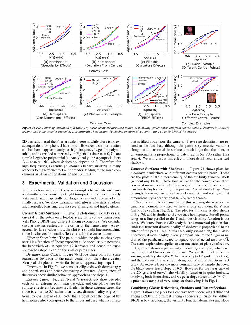
Complex ExamplesFigure 7: Plots showing validation of a variety of scene behaviors discussed in Sec. 3, including glossy reflections from convex objects, shadows in concaveregions, and more complex examples. Dimensionality here means the number of eigenvalues constituting up to 99.95% of the energy.

2D derivation used the Fourier scale theorem, while there is no ex-act equivalent for spherical harmonics. However, a similar relationcan be shown approximately for high-frequency Legendre polyno-mials, and is verified numerically in Fig. 6c,d (since m = 0, Yl0 aresimple Legendre polynomials). Analytically, the asymptotic formPl ∼ cos(lα + Φ), where Φ does not depend on l. Therefore, forhigh frequencies, Legendre polynomials behave similarly in manyrespects to high-frequency Fourier modes, leading to the same con-clusions in 3D as in equations 12 and 13 in 2D.

3 Experimental Validation and DiscussionIn this section, we present several examples to validate our mainresult—that dimensionality of light transport varies almost linearlywith patch size, especially for larger areas (and sub-linearly forsmaller areas). We show examples with glossy materials, shadowsand interreflections, and discuss several insights and implications.

Convex Glossy Surfaces: Figure 7a plots dimensionality vs size(area) A of the patch on a log-log scale for a convex hemispherewith Phong BRDF and different Phong exponents s. We considercircular patches centered at the center of the hemisphere. As ex-pected, for large values of A, the plot is a straight line approachingslope 1, whereas for small A (left of graph), the curve flattens.

Effect of Specularity: The point at which the plot reaches slopenear 1 is a function of Phong exponent s. As specularity s increases,the bandwidth ωG in equation 12 increases and hence the curveapproaches slope 1 earlier, for smaller patch sizes.

Deviation from Centre: Figure 7b shows these plots for somereasonable deviation of the patch center from the sphere center.Nearly all the plots show similar behavior approaching slope 1.

Curvature: In Fig. 7c, we consider ellipsoids with decreasing yand z semi-axes and hence decreasing curvatures. Again, most ofthe curves show similar behavior, approaching the slope 1.

Extreme Cases: Figures 7b and 7c respectively show one ploteach for an extreme point near the edge, and one plot where thesurface effectively becomes a cylinder. In these extreme cases, theslope is closer to 0.5 rather than 1, i.e., dimensionality is propor-tional to

√A instead of A. Note that a point near the edge of the

hemisphere also corresponds to the important case when a surface

that is tilted away from the camera. These rare deviations are re-lated to the fact that, although the patch is symmetric, variationalong one dimension of the surface is much larger than the other, sodimensionality is proportional to patch radius (or

√A) rather than

area A. We will discuss this effect in more detail next, under castshadows.

Concave Surfaces with Shadows: Figure 7d shows plots fora concave hemisphere with different centers for the patch. Theseare the plots of the dimensionality of the visibility function itself(without any BRDF). Note that, unlike for the convex case, thereis almost no noticeable sub-linear region in these curves since thebandwidth ωG for visibility in equation 12 is relatively large. Sur-prisingly however, the curve has a slope of 0.5 and not 1, so thatdimensionality is proportional to

√A, rather than A.

There is a simple explanation for this seeming discrepancy. Acanonical example is where we have a long step along the Y axis(think of extruding Fig. 3c). The plot for this case is also shownin Fig. 7d, and is similar to the concave hemisphere. For all pointslying on a line parallel to the Y axis, the visibility function is thesame. We know from the 2D analysis (and numerical plots in flat-land) that transport dimensionality of shadows is proportional to theextent of the patch—but in this case, only extent along the X axis.Therefore, dimensionality is really proportional to the length or ra-dius of the patch, and hence to square root of actual area or

√A.

The same explanation applies to extreme cases of glossy reflection.Figure 7e shows a particularly interesting example, where we

have a grid of blockers over a plane. We get the black curve byvarying visibility along the X direction only (a 1D grid of blockers),and the red curve by varying it along both X and Y directions (2Dgrid). As expected, for the more common case of simple shadows,the black curve has a slope of 0.5. However for the rarer case ofthe 2D grid (red curve), the visibility function is quite intricate,involving both dimensions, and we get a slope closer to 1.0 (≈ .9)—a practical example of very complex shadowing is in Fig. 1.

Combining Glossy Reflections, Shadows and Interreflections:Figure 7f shows the plots for a concave hemisphere with diffuse andPhong BRDF and different Phong exponents s. Since the diffuseBRDF is low frequency, the visibility function dominates and slope

Clusters for Phong Sphere with Exponent 100

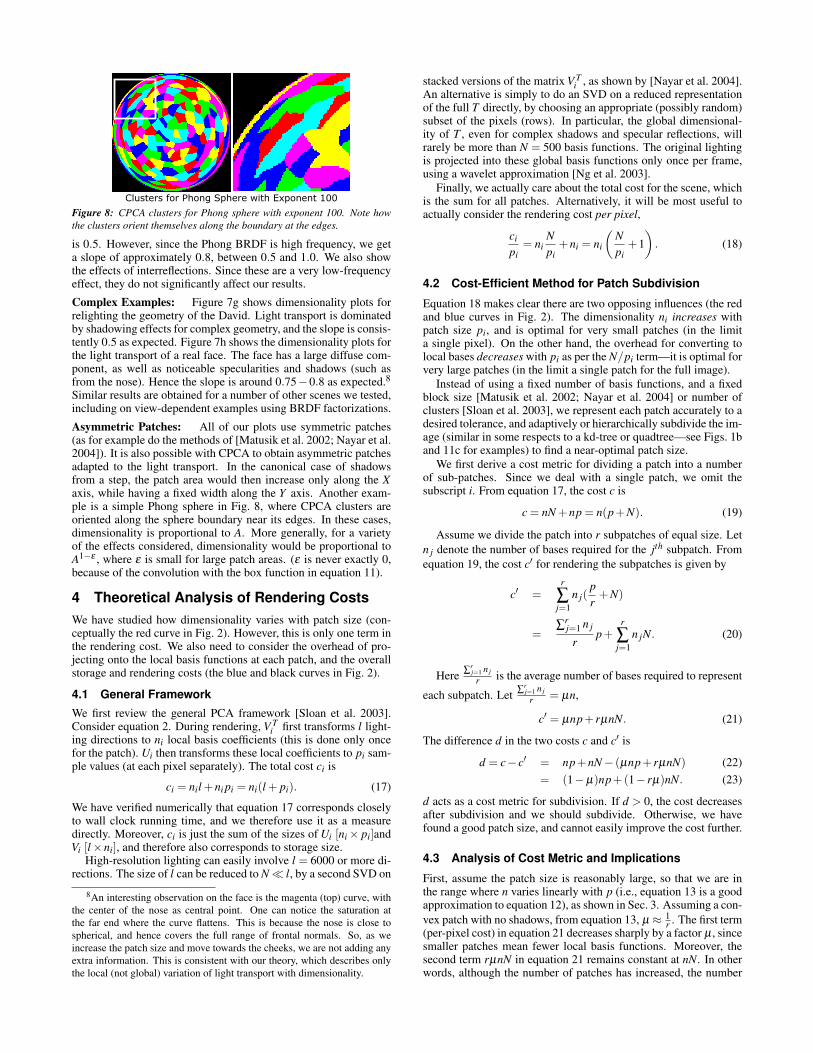
Figure 8: CPCA clusters for Phong sphere with exponent 100. Note howthe clusters orient themselves along the boundary at the edges.

is 0.5. However, since the Phong BRDF is high frequency, we geta slope of approximately 0.8, between 0.5 and 1.0. We also showthe effects of interreflections. Since these are a very low-frequencyeffect, they do not significantly affect our results.

Complex Examples: Figure 7g shows dimensionality plots forrelighting the geometry of the David. Light transport is dominatedby shadowing effects for complex geometry, and the slope is consis-tently 0.5 as expected. Figure 7h shows the dimensionality plots forthe light transport of a real face. The face has a large diffuse com-ponent, as well as noticeable specularities and shadows (such asfrom the nose). Hence the slope is around 0.75−0.8 as expected.8Similar results are obtained for a number of other scenes we tested,including on view-dependent examples using BRDF factorizations.

Asymmetric Patches: All of our plots use symmetric patches(as for example do the methods of [Matusik et al. 2002; Nayar et al.2004]). It is also possible with CPCA to obtain asymmetric patchesadapted to the light transport. In the canonical case of shadowsfrom a step, the patch area would then increase only along the Xaxis, while having a fixed width along the Y axis. Another exam-ple is a simple Phong sphere in Fig. 8, where CPCA clusters areoriented along the sphere boundary near its edges. In these cases,dimensionality is proportional to A. More generally, for a varietyof the effects considered, dimensionality would be proportional toA1−ε , where ε is small for large patch areas. (ε is never exactly 0,because of the convolution with the box function in equation 11).

4 Theoretical Analysis of Rendering CostsWe have studied how dimensionality varies with patch size (con-ceptually the red curve in Fig. 2). However, this is only one term inthe rendering cost. We also need to consider the overhead of pro-jecting onto the local basis functions at each patch, and the overallstorage and rendering costs (the blue and black curves in Fig. 2).

4.1 General FrameworkWe first review the general PCA framework [Sloan et al. 2003].Consider equation 2. During rendering, V T

i first transforms l light-ing directions to ni local basis coefficients (this is done only oncefor the patch). Ui then transforms these local coefficients to pi sam-ple values (at each pixel separately). The total cost ci is

ci = nil +ni pi = ni(l + pi). (17)

We have verified numerically that equation 17 corresponds closelyto wall clock running time, and we therefore use it as a measuredirectly. Moreover, ci is just the sum of the sizes of Ui [ni× pi]andVi [l×ni], and therefore also corresponds to storage size.

High-resolution lighting can easily involve l = 6000 or more di-rections. The size of l can be reduced to N l, by a second SVD on

8An interesting observation on the face is the magenta (top) curve, withthe center of the nose as central point. One can notice the saturation atthe far end where the curve flattens. This is because the nose is close tospherical, and hence covers the full range of frontal normals. So, as weincrease the patch size and move towards the cheeks, we are not adding anyextra information. This is consistent with our theory, which describes onlythe local (not global) variation of light transport with dimensionality.

stacked versions of the matrix V Ti , as shown by [Nayar et al. 2004].

An alternative is simply to do an SVD on a reduced representationof the full T directly, by choosing an appropriate (possibly random)subset of the pixels (rows). In particular, the global dimensional-ity of T , even for complex shadows and specular reflections, willrarely be more than N = 500 basis functions. The original lightingis projected into these global basis functions only once per frame,using a wavelet approximation [Ng et al. 2003].

Finally, we actually care about the total cost for the scene, whichis the sum for all patches. Alternatively, it will be most useful toactually consider the rendering cost per pixel,

ci

pi= ni

Npi

+ni = ni

(Npi

+1)

. (18)

4.2 Cost-Efficient Method for Patch Subdivision

Equation 18 makes clear there are two opposing influences (the redand blue curves in Fig. 2). The dimensionality ni increases withpatch size pi, and is optimal for very small patches (in the limita single pixel). On the other hand, the overhead for converting tolocal bases decreases with pi as per the N/pi term—it is optimal forvery large patches (in the limit a single patch for the full image).

Instead of using a fixed number of basis functions, and a fixedblock size [Matusik et al. 2002; Nayar et al. 2004] or number ofclusters [Sloan et al. 2003], we represent each patch accurately to adesired tolerance, and adaptively or hierarchically subdivide the im-age (similar in some respects to a kd-tree or quadtree—see Figs. 1band 11c for examples) to find a near-optimal patch size.

We first derive a cost metric for dividing a patch into a numberof sub-patches. Since we deal with a single patch, we omit thesubscript i. From equation 17, the cost c is

c = nN +np = n(p+N). (19)

Assume we divide the patch into r subpatches of equal size. Letn j denote the number of bases required for the jth subpatch. Fromequation 19, the cost c′ for rendering the subpatches is given by

c′ =r

∑j=1

n j(pr

+N)

=∑

rj=1 n j

rp+

r

∑j=1

n jN. (20)

Here ∑rj=1 n j

r is the average number of bases required to represent

each subpatch. Let ∑rj=1 n j

r = µn,

c′ = µnp+ rµnN. (21)

The difference d in the two costs c and c′ is

d = c− c′ = np+nN− (µnp+ rµnN) (22)= (1−µ)np+(1− rµ)nN. (23)

d acts as a cost metric for subdivision. If d > 0, the cost decreasesafter subdivision and we should subdivide. Otherwise, we havefound a good patch size, and cannot easily improve the cost further.

4.3 Analysis of Cost Metric and Implications

First, assume the patch size is reasonably large, so that we are inthe range where n varies linearly with p (i.e., equation 13 is a goodapproximation to equation 12), as shown in Sec. 3. Assuming a con-vex patch with no shadows, from equation 13, µ ≈ 1

r . The first term(per-pixel cost) in equation 21 decreases sharply by a factor µ , sincesmaller patches mean fewer local basis functions. Moreover, thesecond term rµnN in equation 21 remains constant at nN. In otherwords, although the number of patches has increased, the number

4 8 16 32 64 1280

40

80

120co

st p

er p

ixel

patch size(square side)

nN/pnc/p = n + nN/p(total cost)

minima (p ~ 170)

26.7

0 200 400 600 800 1000number of clusters

5.0

15.0

25.0

35.0

cost

per

pix

el

nN/pnc/p = n + nN/p

p ~ 17020.9

0

.2

.4

.6

.8

1

0 100 200 300 400

(a) Cost plot - blockwise PCA (b) Cost plot - CPCA (c) Cost comparison for scaling (d) Histogram (e) Histogram (256 X 256 image) (256 X 256 image) with resolution (256 X 256 image) (128 X 128 image)

cluster size

**

100 300 500 700

5

7

9

11

4.2

8.0

p ~ 170

p ~ 140

*

*

average cluster size (p) 0 100 200 300 4000

.2

.4

.6

.8

1

cluster size

freq

uen

cy

e+5256 x 256 image

128x128 image

Cost Curves

Scaling of Cost with Resolution (CPCA)Cost vs Patch Size

freq

uen

cy

tota

l re

nder

ing c

ost

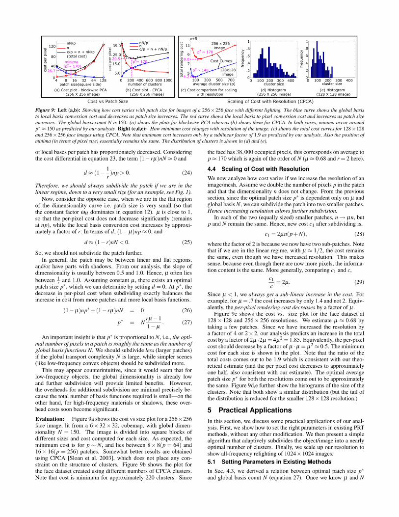
Figure 9: Left (a,b): Showing how cost varies with patch size for images of a 256× 256 face with different lighting. The blue curve shows the global basisto local basis conversion cost and decreases as patch size increases. The red curve shows the local basis to pixel conversion cost and increases as patch sizeincreases. The global basis count N is 150. (a) shows the plots for blockwise PCA whereas (b) shows them for CPCA. In both cases, minima occur aroundp∗ ≈ 150 as predicted by our analysis. Right (c,d,e): How minimum cost changes with resolution of the image. (c) shows the total cost curves for 128×128and 256×256 face images using CPCA. Note that minimum cost increases only by a sublinear factor of 1.9 as predicted by our analysis. Also the position ofminima (in terms of pixel size) essentially remains the same. The distribution of clusters is shown in (d) and (e).

of local bases per patch has proportionately decreased. Consideringthe cost differential in equation 23, the term (1− rµ)nN ≈ 0 and

d ≈ (1− 1r)np > 0. (24)

Therefore, we should always subdivide the patch if we are in thelinear regime, down to a very small size (for an example, see Fig. 1).

Now, consider the opposite case, when we are in the flat regionof the dimensionality curve i.e. patch size is very small (so thatthe constant factor ωH dominates in equation 12). µ is close to 1,so that the per-pixel cost does not decrease significantly (remainsat np), while the local basis conversion cost increases by approxi-mately a factor of r. In terms of d, (1−µ)np≈ 0, and

d ≈ (1− r)nN < 0. (25)

So, we should not subdivide the patch further.In general, the patch may be between linear and flat regions,

and/or have parts with shadows. From our analysis, the slope ofdimensionality is usually between 0.5 and 1.0. Hence, µ often liesbetween 1

r and 1.0. Assuming constant µ , there exists an optimalpatch size p∗, which we can determine by setting d = 0. At p∗, thedecrease in per-pixel cost when subdividing exactly balances theincrease in cost from more patches and more local basis functions.

(1−µ)np∗+(1− rµ)nN = 0 (26)

p∗ = Nrµ−11−µ

. (27)

An important insight is that p∗ is proportional to N, i.e., the opti-mal number of pixels in a patch is roughly the same as the number ofglobal basis functions N. We should subdivide less (larger patches)if the global transport complexity N is large, while simpler scenes(like low-frequency convex objects) should be subdivided more.

This may appear counterintuitive, since it would seem that forlow-frequency objects, the global dimensionality is already lowand further subdivision will provide limited benefits. However,the overheads for additional subdivision are minimal precisely be-cause the total number of basis functions required is small—on theother hand, for high-frequency materials or shadows, these over-head costs soon become significant.

Evaluation: Figure 9a shows the cost vs size plot for a 256×256face image, lit from a 6× 32× 32, cubemap, with global dimen-sionality N = 150. The image is divided into square blocks ofdifferent sizes and cost computed for each size. As expected, theminimum cost is for p ∼ N, and lies between 8× 8(p = 64) and16× 16(p = 256) patches. Somewhat better results are obtainedusing CPCA [Sloan et al. 2003], which does not place any con-straint on the structure of clusters. Figure 9b shows the plot forthe face dataset created using different numbers of CPCA clusters.Note that cost is minimum for approximately 220 clusters. Since

the face has 38,000 occupied pixels, this corresponds on average top≈ 170 which is again of the order of N (µ ≈ 0.68 and r = 2 here).

4.4 Scaling of Cost with ResolutionWe now analyze how cost varies if we increase the resolution of animage/mesh. Assume we double the number of pixels p in the patchand that the dimensionality n does not change. From the previoussection, since the optimal patch size p∗ is dependent only on µ andglobal basis N, we can subdivide the patch into two smaller patches.Hence increasing resolution allows further subdivision.

In each of the two (equally sized) smaller patches, n → µn, butp and N remain the same. Hence, new cost c1 after subdividing is,

c1 = 2µn(p+N), (28)

where the factor of 2 is because we now have two sub-patches. Notethat if we are in the linear regime, with µ ≈ 1/2, the cost remainsthe same, even though we have increased resolution. This makessense, because even though there are now more pixels, the informa-tion content is the same. More generally, comparing c1 and c,

c1

c= 2µ. (29)

Since µ < 1, we always get a sub-linear increase in the cost. Forexample, for µ = .7 the cost increases by only 1.4 and not 2. Equiv-alently, the per-pixel rendering cost decreases by a factor of µ .

Figure 9c shows the cost vs. size plot for the face dataset at128× 128 and 256× 256 resolutions. We estimate µ ≈ 0.68 bytaking a few patches. Since we have increased the resolution bya factor of 4 or 2× 2, our analysis predicts an increase in the totalcost by a factor of 2µ ·2µ = 4µ2 = 1.85. Equivalently, the per-pixelcost should decrease by a factor of µ ·µ = µ2 ≈ 0.5. The minimumcost for each size is shown in the plot. Note that the ratio of thetotal costs comes out to be 1.9 which is consistent with our theo-retical estimate (and the per pixel cost decreases to approximatelyone half, also consistent with our estimate). The optimal averagepatch size p∗ for both the resolutions come out to be approximatelythe same. Figure 9d,e further show the histograms of the size of theclusters. Note that both show a similar distribution (but the tail ofthe distribution is reduced for the smaller 128×128 resolution.)

5 Practical ApplicationsIn this section, we discuss some practical applications of our anal-ysis. First, we show how to set the right parameters in existing PRTmethods, without any other modification. We then present a simplealgorithm that adaptively subdivides the object/image into a nearlyoptimal number of clusters. Finally, we scale up our resolution toshow all-frequency relighting of 1024×1024 images.5.1 Setting Parameters in Existing MethodsIn Sec. 4.3, we derived a relation between optimal patch size p∗and global basis count N (equation 27). Once we know µ and N

Frame Rate = 45 Hz Frame Rate = 125 Hz

(a) Image Relighting (b) Surface Light Fields

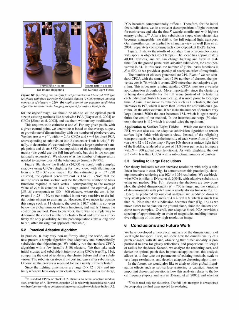
Figure 10: (a) Using our analysis to set parameters in Clustered PCA (forrelighting with fixed view) for the Buddha dataset (24,000 vertices, optimalnumber m of clusters = 220). (b) Application of our adaptive subdivisionalgorithm to render with changing viewpoint for surface light fields.

for the object/image, we should be able to set the optimal patchsize in existing methods like blockwise PCA [Nayar et al. 2004] orCPCA [Sloan et al. 2003], and use them without any modification.

This requires us to estimate µ and N. For any given patch, witha given central point, we determine µ based on the average slope sor growth rate of dimensionality with the number of pixels/vertices.We then use µ = r−s, with r = 2 for CPCA and r = 4 for block PCA(corresponding to subdivision into 2 clusters or 4 sub-blocks).9 Fi-nally, to determine N, we randomly choose a large number of sam-ple points and do an SVD decomposition of the resulting transportmatrix (we could use the full image/mesh, but this is too compu-tationally expensive). We choose N as the number of eigenvectorsneeded to capture most of the total energy (usually 99.9%).

Figure 10a shows the Buddha (24,000 vertices), with complexshadows using CPCA relighting for fixed view, with illuminationfrom 6× 32× 32 cube maps. For the estimated µ = .57 (220clusters), the optimal per-vertex cost is 114.78. (Note that theunit of costs in this section will be the effective number of basisfunctions required at each vertex—corresponding to the averagevalue of c/p in equation 18.) A range around the optimal µ of[.53, .6] corresponds to 130− 600 clusters, where the cost is be-tween 114.78−130, so our method is not very sensitive to the ini-tial points chosen to estimate µ . However, if we move far outsidethis range such as 11 clusters, the cost is 310.7 which is not evenbelow the global number of basis functions, and nearly 3 times thecost of our method. Prior to our work, there was no simple way todetermine the correct number of clusters (trial and error was effec-tively the only possibility, but the precomputations take a long timeto run, often making that approach infeasible).

5.2 Practical Adaptive Algorithm

In practice, µ may vary non-uniformly along the scene, and wenow present a simple algorithm that adaptively and hierarchicallysubdivides the object/image. We initially run the standard CPCAalgorithm with a few (usually 5-10) clusters. We then take eachinitial cluster, and subdivide it into two using CPCA (see Fig. 11c),comparing the cost of rendering the cluster before and after subdi-vision. The subdivision stops if the cost increases after subdivision.Otherwise, the process is repeated for each newly formed cluster.

Since the lighting dimensions are large (6× 32× 32), and ini-tially when we have only a few clusters, the cluster size is also large,

9In standard CPCA or block PCA, there is no actual adaptive subdivi-sion, or notion of r. However, equation 27 is relatively insensitive to r, andwe therefore use values corresponding to our adaptive technique in Sec. 5.2.

PCA becomes computationally difficult. Therefore, for the initialfew subdivisions, we do a wavelet decomposition of light transportfor each vertex and take the first K wavelet coefficients with highestenergy globally.10 After a few subdivision steps, when cluster sizebecomes manageable, we shift to the full original light transport.Our algorithm can be applied to changing view as well [Liu et al.2004], separately considering each view-dependent BRDF factor.

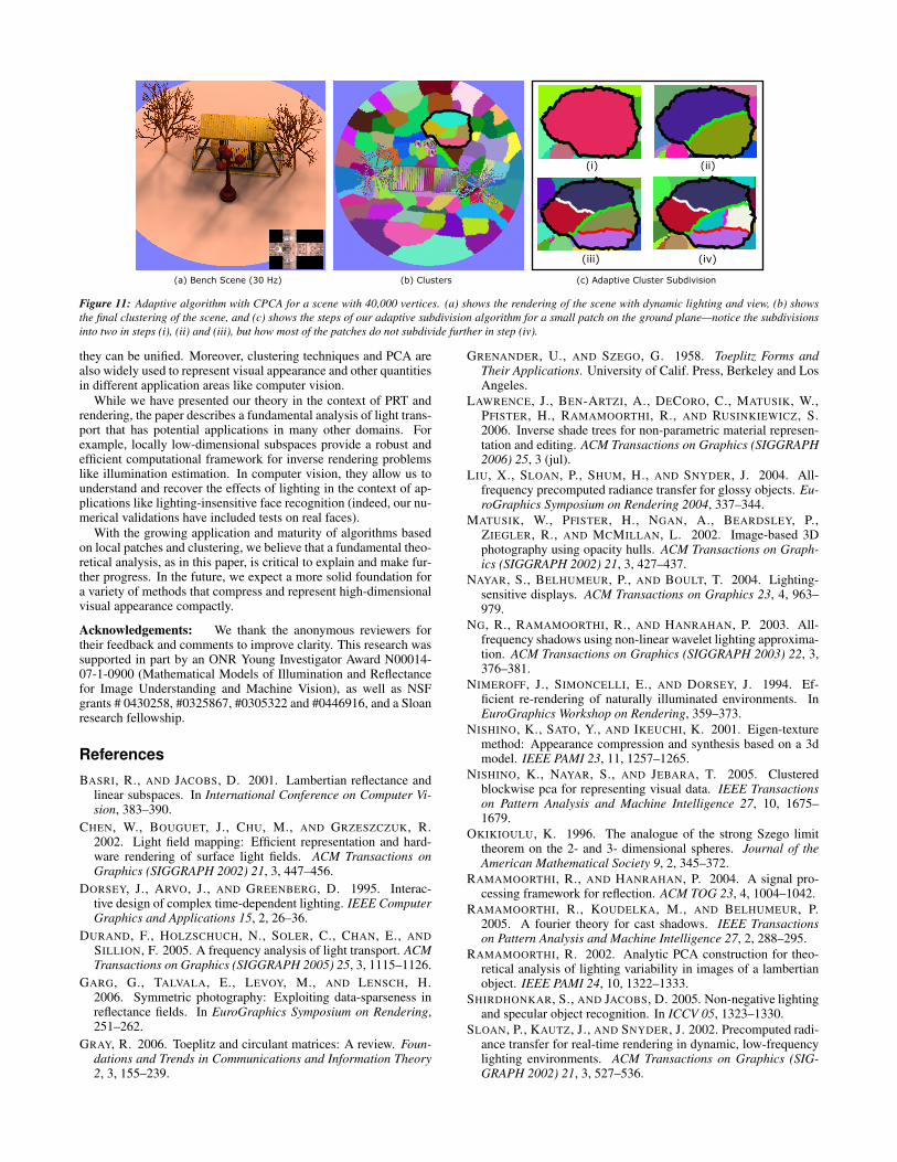
Figure 11 shows the results of our algorithm on a complex scenewith specular objects (street lamps). The scene has approximately40,000 vertices, and we can change lighting and view in real-time. For the ground plane, with adpative subdivison, the cost (per-vertex) is 64. In this case, the number of global basis functions isN = 500, so we provide a speedup of nearly an order of magnitude.

The number of clusters generated are 219. Even if we run stan-dard CPCA with the same fixed (219) number of clusters, the per-vertex cost is 76, which is around 20% more than our adaptive algo-rithm. This is because running standard CPCA must use a waveletapproximation throughout. More importantly, since the clusteringis being done globally for the full scene (instead of reclusteringeach individual cluster hierarchically), it is more prone to local op-tima. Again, if we move to extremes such as 10 clusters, the costincreases to 197, which is more than 3 times the cost with our algo-rithm. At the other extreme, if we make the number of clusters verylarge (around 5000) the cost becomes 184, which is again nearlythrice the cost of our method. In the intermediate range (50 clus-ters), the cost is 112 which is around twice the optimum.

Application to Surface Light Fields: While our main focus isPRT, we can also use the adaptive subdivision algorithm to rendersurface light fields with dynamic view. Instead of the relightingtransport matrix, we have the intensity of each vertex from all views(on a 6×32×32 cube map.) Figure 10b shows a surface light fieldof the Buddha, rendered at a cost of 31.8 bases per vertex (comparewith N = 300 global basis functions). As with relighting, the costis 3×–4× less than CPCA with a sub-optimal number of clusters.

5.3 Scaling to Large Resolutions

Our theory indicates we can increase resolution with only a sub-linear increase in cost. Fig. 1a demonstrates this practically, show-ing interactive rendering at a 1024×1024 resolution. We use block-wise PCA (similar to [Nayar et al. 2004]), with adaptive subdivisionusing our method (Fig. 1b). Because the shadows are very com-plex, the global dimensionality N = 700 is large, and the variationof dimensionality with patch size is nearly always linear in Fig. 1c.Hence, as predicted by our cost analysis, we subdivide down tovery small patches with areas of 4×4 or 8×8, which is much lessthan N. Note that the subdivision becomes finer (Fig. 1b) as wemove closer to the plant on the ground plane, since the shadows be-come more complex. Overall, our adaptive block PCA provides aspeedup of approximately an order of magnitude, enabling interac-tive relighting of this very high-resolution image.

6 Conclusions and Future WorkWe have developed a theoretical analysis of the dimensionality oflocal light transport. First, we show how the dimensionality of apatch changes with its size, observing that dimensionality is pro-portional to area for glossy reflections, and proportional to lengthor radius for shadows. Second, we analyze the rendering cost, andderive the optimal patch size. In practical applications, this analysisallows us to fine tune the parameters of existing methods, scale tovery large resolutions, and develop adaptive clustering algorithms.

In the future, we would also like to analyze other global illumi-nation effects such as sub-surface scattering or caustics. Anotherimportant theoretical question is how this analysis relates to the lo-cal frequency-space analysis in [Durand et al. 2005], and whether

10This is used only for clustering. The full light transport is always usedfor computing the final bases needed for rendering.

(a) Bench Scene (30 Hz) (b) Clusters (c) Adaptive Cluster Subdivision

(i) (ii)

(iii) (iv)

Figure 11: Adaptive algorithm with CPCA for a scene with 40,000 vertices. (a) shows the rendering of the scene with dynamic lighting and view, (b) showsthe final clustering of the scene, and (c) shows the steps of our adaptive subdivision algorithm for a small patch on the ground plane—notice the subdivisionsinto two in steps (i), (ii) and (iii), but how most of the patches do not subdivide further in step (iv).

they can be unified. Moreover, clustering techniques and PCA arealso widely used to represent visual appearance and other quantitiesin different application areas like computer vision.

While we have presented our theory in the context of PRT andrendering, the paper describes a fundamental analysis of light trans-port that has potential applications in many other domains. Forexample, locally low-dimensional subspaces provide a robust andefficient computational framework for inverse rendering problemslike illumination estimation. In computer vision, they allow us tounderstand and recover the effects of lighting in the context of ap-plications like lighting-insensitive face recognition (indeed, our nu-merical validations have included tests on real faces).

With the growing application and maturity of algorithms basedon local patches and clustering, we believe that a fundamental theo-retical analysis, as in this paper, is critical to explain and make fur-ther progress. In the future, we expect a more solid foundation fora variety of methods that compress and represent high-dimensionalvisual appearance compactly.

Acknowledgements: We thank the anonymous reviewers fortheir feedback and comments to improve clarity. This research wassupported in part by an ONR Young Investigator Award N00014-07-1-0900 (Mathematical Models of Illumination and Reflectancefor Image Understanding and Machine Vision), as well as NSFgrants # 0430258, #0325867, #0305322 and #0446916, and a Sloanresearch fellowship.

ReferencesBASRI, R., AND JACOBS, D. 2001. Lambertian reflectance and

linear subspaces. In International Conference on Computer Vi-sion, 383–390.

CHEN, W., BOUGUET, J., CHU, M., AND GRZESZCZUK, R.2002. Light field mapping: Efficient representation and hard-ware rendering of surface light fields. ACM Transactions onGraphics (SIGGRAPH 2002) 21, 3, 447–456.

DORSEY, J., ARVO, J., AND GREENBERG, D. 1995. Interac-tive design of complex time-dependent lighting. IEEE ComputerGraphics and Applications 15, 2, 26–36.

DURAND, F., HOLZSCHUCH, N., SOLER, C., CHAN, E., ANDSILLION, F. 2005. A frequency analysis of light transport. ACMTransactions on Graphics (SIGGRAPH 2005) 25, 3, 1115–1126.

GARG, G., TALVALA, E., LEVOY, M., AND LENSCH, H.2006. Symmetric photography: Exploiting data-sparseness inreflectance fields. In EuroGraphics Symposium on Rendering,251–262.

GRAY, R. 2006. Toeplitz and circulant matrices: A review. Foun-dations and Trends in Communications and Information Theory2, 3, 155–239.

GRENANDER, U., AND SZEGO, G. 1958. Toeplitz Forms andTheir Applications. University of Calif. Press, Berkeley and LosAngeles.

LAWRENCE, J., BEN-ARTZI, A., DECORO, C., MATUSIK, W.,PFISTER, H., RAMAMOORTHI, R., AND RUSINKIEWICZ, S.2006. Inverse shade trees for non-parametric material represen-tation and editing. ACM Transactions on Graphics (SIGGRAPH2006) 25, 3 (jul).

LIU, X., SLOAN, P., SHUM, H., AND SNYDER, J. 2004. All-frequency precomputed radiance transfer for glossy objects. Eu-roGraphics Symposium on Rendering 2004, 337–344.

MATUSIK, W., PFISTER, H., NGAN, A., BEARDSLEY, P.,ZIEGLER, R., AND MCMILLAN, L. 2002. Image-based 3Dphotography using opacity hulls. ACM Transactions on Graph-ics (SIGGRAPH 2002) 21, 3, 427–437.

NAYAR, S., BELHUMEUR, P., AND BOULT, T. 2004. Lighting-sensitive displays. ACM Transactions on Graphics 23, 4, 963–979.

NG, R., RAMAMOORTHI, R., AND HANRAHAN, P. 2003. All-frequency shadows using non-linear wavelet lighting approxima-tion. ACM Transactions on Graphics (SIGGRAPH 2003) 22, 3,376–381.

NIMEROFF, J., SIMONCELLI, E., AND DORSEY, J. 1994. Ef-ficient re-rendering of naturally illuminated environments. InEuroGraphics Workshop on Rendering, 359–373.

NISHINO, K., SATO, Y., AND IKEUCHI, K. 2001. Eigen-texturemethod: Appearance compression and synthesis based on a 3dmodel. IEEE PAMI 23, 11, 1257–1265.

NISHINO, K., NAYAR, S., AND JEBARA, T. 2005. Clusteredblockwise pca for representing visual data. IEEE Transactionson Pattern Analysis and Machine Intelligence 27, 10, 1675–1679.

OKIKIOULU, K. 1996. The analogue of the strong Szego limittheorem on the 2- and 3- dimensional spheres. Journal of theAmerican Mathematical Society 9, 2, 345–372.

RAMAMOORTHI, R., AND HANRAHAN, P. 2004. A signal pro-cessing framework for reflection. ACM TOG 23, 4, 1004–1042.

RAMAMOORTHI, R., KOUDELKA, M., AND BELHUMEUR, P.2005. A fourier theory for cast shadows. IEEE Transactionson Pattern Analysis and Machine Intelligence 27, 2, 288–295.

RAMAMOORTHI, R. 2002. Analytic PCA construction for theo-retical analysis of lighting variability in images of a lambertianobject. IEEE PAMI 24, 10, 1322–1333.

SHIRDHONKAR, S., AND JACOBS, D. 2005. Non-negative lightingand specular object recognition. In ICCV 05, 1323–1330.

SLOAN, P., KAUTZ, J., AND SNYDER, J. 2002. Precomputed radi-ance transfer for real-time rendering in dynamic, low-frequencylighting environments. ACM Transactions on Graphics (SIG-GRAPH 2002) 21, 3, 527–536.

SLOAN, P., HALL, J., HART, J., AND SNYDER, J. 2003. Clusteredprincipal components for precomputed radiance transfer. ACMTransactions on Graphics (SIGGRAPH 2003) 22, 3, 382–391.

SOLER, C., AND SILLION, F. 1998. Fast calculation of soft shadowtextures using convolution. In SIGGRAPH 98, 321–332.

WANG, R., TRAN, J., AND LUEBKE, D. 2006. All-frequencyrelighting of glossy objects. ACM Transactions on Graphics 25,2, 293–318.