NBER WORKING PAPER SERIES

A THEORY OF OUTSOURCING AND WAGE DECLINE

Thomas J. HolmesJulia Thornton Snider

Working Paper 14856http://www.nber.org/papers/w14856

NATIONAL BUREAU OF ECONOMIC RESEARCH1050 Massachusetts Avenue

Cambridge, MA 02138April 2009

Holmes acknowledges NSF Grant 0551062 for support of this research. We thank Erzo Luttmer andCharles Thomas and workshop participants at the University of Minnesota for helpful comments onthis paper. The views expressed herein are those of the authors and not necessarily those of the FederalReserve Bank of Minneapolis, the Federal Reserve System, or the National Bureau of Economic Research.

NBER working papers are circulated for discussion and comment purposes. They have not been peer-reviewed or been subject to the review by the NBER Board of Directors that accompanies officialNBER publications.

© 2009 by Thomas J. Holmes and Julia Thornton Snider. All rights reserved. Short sections of text,not to exceed two paragraphs, may be quoted without explicit permission provided that full credit,including © notice, is given to the source.

A Theory of Outsourcing and Wage DeclineThomas J. Holmes and Julia Thornton SniderNBER Working Paper No. 14856April 2009JEL No. J31,L22,L23

ABSTRACT

We develop a theory of outsourcing in which there is market power in one factor market (labor) andno market power in a second factor market (capital). There are two intermediate goods: one labor-intensiveand the other capital-intensive. We show there is always outsourcing in the market allocation whena friction limiting outsourcing is not too big. The key factor underlying the result is that labor demandis more elastic, the greater the labor share. Integrated plants pay higher wages than the specialist producersof labor-intensive intermediates. We derive conditions under which there are multiple equilibria thatvary in the degree of outsourcing. Across these equilibria, wages are lower the greater the degree ofoutsourcing. Wages fall when outsourcing increases in response to a decline in the outsourcing friction.¸

Thomas J. HolmesDepartment of EconomicsUniversity of Minnesota4-101 Hanson Hall1925 Fourth Street SouthMinneapolis, MN 55455and The Federal Reserve Bank of Minneapolis and NBERholmes@umn.edu

Julia Thornton SniderDept of Economics, Univ of Minnesota4-101 Hanson Hall, 1925 4th St SMinneapolis, MN 55455and The Federal Reserve Bank of Minneapolisthornton@umn.edu

1 Introduction

In the 1920s, Henry Ford famously built a factory in which the raw materials for steel went

in on one end and finished automobiles went out the other. Extreme vertical integration like

this is not the fashion today. Ford Motor has in recent years spun off a significant portion

of its parts-making operations as a separate company, and General Motors has done the

same. Within its assembly plants, General Motors is currently trying to outsource janitorial

services and forklift operations to outside contractors.

This paper develops a theory of outsourcing in which the circumstances under which

factors of production can grab rents play the leading role. One factor has some monopoly

power (call this labor) while a second factor does not (call this capital). There are two stages

of production: a labor-intensive task and a capital-intensive task. For example, auto part

production (such as hand soldering of wire harnesses) tends to be labor-intensive, while final

assembly of automobiles (with robots and huge machines) tends to be capital-intensive. In

the model, all firms have the same abilities, so there is no motivation to specialize to exploit

Ricardian comparative advantage. Furthermore, an outsourcing friction is incurred when

the two tasks are not integrated in the same firm. So, in the absence of any monopoly power

by labor, all firms are completely integrated, doing the labor-intensive and capital-intensive

tasks as part of the same operation, and the outsourcing friction is avoided. However, if

labor has monopoly power and if the friction is not too large, outsourcing necessarily takes

place, with some firms specializing in the labor-intensive task and other firms specializing in

the capital-intensive task.

The mechanism underlying our outsourcing result is simply that labor demand is more

elastic, the greater the labor share of a firm’s overall factor bill. In particular, the demand of

an integrated firm is less elastic than the demand of a specialist labor-intensive producer, such

as a janitorial services provider. Therefore, a monopolist selling labor to a labor-intensive

firm will choose a lower wage than one selling to an integrated plant. This wage difference is

the force driving the disintegration of production of the high and low labor-intensity tasks.

(But note the wage of a specialist capital-intensive plant is higher than for an integrated

plant. This is a subtlety we return to below.)

The main question that we address with the model is: How are changes in outsourcing re-

lated to changes in wage payments in general equilibrium? Our unambiguous finding is that

increases in outsourcing go hand in hand with decreases in wage payments. Our result allows

for two forces underlying an increase in outsourcing. The first force is a decrease over time

in the outsourcing friction. A recent series of papers, including Antràs, Garicano, and Rossi-

Hansberg (2006) and Grossman and Rossi-Hansberg (2008), have emphasized the advances

in information and transportation technology that have permitted the separation of tasks

previously required to be part of the same operation. When components are manufactured

by separate operations, information costs must be incurred to ensure that separately pro-

duced components fit together both physically and in a timely production schedule (such as

in just-in-time production). Japanese automobile manufacturers pioneered new ways to co-

ordinate production with suppliers (see Womack, Jones, and Roos (1990) and Mair, Florida,

and Kenney (1988)), and these methods have been adopted by U.S. manufacturers. This is

an example of a decrease in the outsourcing friction. In recent years, there have been inno-

vations in organizational forms and administrative structures, such as professional employer

organizations that facilitate the segmentation of factors of production across different firm

boundary lines. We broadly interpret these innovations as decreases in the friction.

The second force potentially underlying an increase in outsourcing is a positive feedback

between lower wages and more outsourcing. This makes it possible to observe different

outcomes over time, even when technological fundamentals do not change. That is, for certain

parameters in our model, there can be multiple equilibria with different levels of outsourcing.

When this happens, we show the equilibria can be ordered so that more outsourcing is

associated with lower average wages. Put in another way, an increase in outsourcing can

depress wages in general equilibrium which, in turn, can change incentives so that firms

want to do more outsourcing, making the original increase in outsourcing self-reinforcing.

We find that the possibility of multiple equilibria is contingent on an assumption that rent-

seeking activity (for union rents) absorbs a portion of the labor supply, putting upward

pressure on wages. Our finding that for the same model parameters both an outsourcing

and a vertical integration equilibrium might exist is reminiscent of a finding by McLaren

(2000). But the mechanism and context are completely different here.

A premise of this paper is that labor has market power while capital does not. There

are good reasons to accept this premise. Workers can go on strike, and various job market

protections in labor law can enhance labor bargaining power. Perhaps there will come a

day when robots go on strike, but for now, business managers need not worry about capital

walking off the job. In the formal analysis, we model market power narrowly as taking

the form of a union with a monopoly on labor at the plant level. Our idea applies more

broadly to include other sources of market power for workers, including job search frictions

and potentially even social norms. Finally, while we call factor one labor and factor two

2

capital, we can just as easily think of factor one as unionized unskilled labor and factor two

as nonunion skilled labor.

Whether to integrate or outsource–the “make or buy” decision–is a classic topic in the

theory of the firm. Much of the literature has focused on the role of incomplete contracts

(Williamson (1979), Grossman and Hart (1986)).1 In these models, economic agents cannot

contractually commit to future behavior. Firm boundaries are drawn to optimally influence

incentives, given the constraints of incomplete contracts. This kind of timing and commit-

ment issue arises in our model. We make a crucial assumption that firms make long-run

decisions about integration status before they engage in wage negotiations; the anticipation

of lower wages on the labor-intensive task is precisely what induces firms to outsource. While

our paper follows this literature in that timing and commitment play a key role, the model

we consider is very different from those in the existing literature. This is especially true in

the way we highlight and incorporate differences in factor composition across tasks Also, the

main question we address, How does outsourcing impact wages in general equilibrium? is

different from the standard topic in the incomplete contracts literature, which is: When and

how does outsourcing occur?

In its general equilibrium approach and its focus on what happens when trade frictions

decline, the paper is close in spirit to the trade literature on offshoring (e.g., Grossman and

Helpman (2005), Antràs, Garicano, and Rossi-Hansberg (2006)) and assignment theories

of foreign direct investment (FDI) about who should specialize in which task (Nocke and

Yeaple (2008)).2 Our paper is particularly related to Grossman and Rossi-Hansberg (2008).

That paper highlights how a reduction in an outsourcing friction can potentially raise low-

skill wages in a high-skill country through what they call a productivity effect. This effect

operates through a fixed amount of outsourcing proceeding more efficiently on account of

the technical change. This channel operates in our model as well. Fixing the extent of

outsourcing at some positive level, a reduction in the outsourcing friction raises wages as

workers share the benefit of technological improvements. The negative impact on wages

from technical change in our model comes entirely from its impact on increasing the extent

of outsourcing.

The tensions that exist in our model are related to issues that arise in the analysis of price

discrimination. With integration, there is a uniform wage for labor. With outsourcing, there

1A more recent literature examines how information flows affect integration decisions (Alonso, Dessein,

and Matouschek (2008), Friebel and Raith (2006)).2See also Liao (2009) for the analogous impact in an urban economics model.

3

is one wage for workers who do the labor-intensive task and a second, higher wage for workers

who do the capital-intensive task. The uniform wage under outsourcing lies between the two

task-specific, discriminatory wages. In the standard decision-theoretic analysis of monopoly

price discrimination, a monopolist is always better off when price discrimination is feasible.

However, as shown in Holmes (1989) and Corts (1998), the ability to price discriminate

in a competitive context can potentially reduce equilibrium returns to price discriminators.

In an analogous way, unions in our model are worse off in equilibrium when workers doing

different tasks receive different wages because of outsourcing. As noted parenthetically above,

wage levels and total wage payments to workers doing the capital-intensive task actually do

increase with outsourcing compared to integration. But we show that these gains are more

than offset by losses suffered by workers doing the labor-intensive task.

Existing empirical research provides evidence that wage reductions play a role in motivat-

ing outsourcing decisions. The building service industry (i.e., janitorial services) is obviously

a labor-intensive industry. Abraham (1990) and Dube and Kaplan (2008) show that build-

ing service employees employed in the business service sector (e.g., contract cleaning firms)

receive substantially lower wages and benefits than employees doing the same jobs and with

similar characteristics employed by manufacturing firms. And Abraham and Taylor (1996)

show that it is the higher-wage firms that are more likely to contract out cleaning services.

Forbes and Lederman (forthcoming) discuss how airlines spin off short routes to regional

airlines because the pilots of these airlines are then less able to extract rents. This fits our

model if short routes with small planes are less capital intensive than long-haul routes with

large planes. Doellgast and Greer (2007) provide a case study of the German automobile

industry to show how outsourcing parts has cut rents. We do not know of such a study

for the U.S. automobile industry, but as mentioned in the first paragraph, there is anecdo-

tal evidence that the same has happened in the United States. More specifically, General

Motors (GM) spun off Delphi, its labor-intensive parts operations, and subsequently Delphi

is trying to cut wages “to as little as $10 an hour from as much as $30.”3 GM spun off

the parts operation American Axle in 1992, and subsequently American Axle succeeded in

cutting wages by about a third.4 As part of the plan to outsource janitorial services at GM

assembly plants, the expectation is that wages to janitors would fall from $28 an hour for an

in-house GM employee to around $12 an hour for an employee of a contract cleaning firm.5

3The quote is from the New York Times, November 19, 2005, “For a G.M. Family, the American Dream

Vanishes,” by Danny Hakim.4See “American Axle Contract Ratified, Strike Ends,” Reuters, May 22, 2008.5See “GM to UAW: Let’s Cut Costs,” Workforce Management: News in Brief, April 16, 2007.

4

The remainder of the paper is organized as follows. Section 2 lays out the model, and

Section 3 works out what happens when wages are fixed. Section 4 is the main analysis

determining the link between outsourcing and wages. Section 5 concludes.

2 Model

We describe the technology and then explain how unions operate. Next we explain timing

in the model and define equilibrium.

2.1 The Technology

We model an industry in which a final good is made out of two intermediates. The first

is labor-intensive (intermediate 1). The other is capital-intensive (intermediate 2). Let

denote a quantity of intermediate .

A firm may be vertically integrated, producing both intermediates and combining them

on its premises. Or it can be specialized in the production of a particular intermediate good.

The final good results from combining the two intermediates according to a fixed-proportions

technology. If the two inputs 1 and 2 are produced in a vertically integrated firm, then

final good output equals

= (1 2) = min {1 2} . (1)

If the inputs are produced by two specialists, then final good output is

= (1 2) = (1− )min {1 2} .

The parameter ≥ 0 is the outsourcing friction that must be incurred when the two stepsof production are undertaken by two different firms.

To illustrate the friction , suppose that if the two steps are undertaken by separate

firms, the intermediates need to be wrapped in certain protective packaging before being

shipped off to final assembly. An integrated plant making both intermediates and combining

them on premises can avoid the packaging process. In this illustrative case, represents

the physical cost of wrapping and unwrapping the intermediates as well as the cost of the

packing materials. In addition to physical costs like these, as discussed in the introduction

we interpret broadly as representing costs of coordinating production. Recent advances in

5

information and transportation technology have substantially lowered such costs; i.e., has

decreased.

The three factors of production in the economy are: managers, labor, and capital. There

is a unit measure of managers who each own one firm. Given the one-to-one relationship,

for simplicity, will refer to the combination of one manager and one firm as a “firm.” There

is a measure of labor that is supplied inelastically to the economy. There is a perfectly

elastic supply of capital to the economy at a rental price of per unit.

Each firm has access to the same technology for converting capital and labor into in-

termediates. Let (1 1 2 2) denote an input vector for a particular firm, where and

denote the amount of capital and labor the firm allocates to the production of intermediate

. Given such an input vector, the production levels for each intermediate equal

1 = 1 (1 + 2)−(1−)

(2)

2 = 2 (1 + 2)−(1−)

where is the composite input for intermediate i defined by

= ( ) =1

(1− )

1− 1− . (3)

To understand this technology, observe that the and are first combined in a constant-

returns Cobb-Douglas fashion through (3) to create a composite input . Then 1 and 2

are run through (2) to determine the intermediate production levels 1 and 2. This last

step allows for diminishing marginal product where the level of curvature is governed by the

parameter . If = 1, then = , and we have constant returns to scale in the relationship

between capital and labor and the intermediate outputs. We assume ∈ (0 1), whichimplies diminishing returns. Note the degree of diminishing returns in (3) is determined

by the total composite input 1 + 2. An increase in production of one intermediate lowers

the marginal product of the other intermediate. Finally, we emphasize that in addition to

the explicit vector of inputs (1 1 2 2) in the technology above, there is also implicitly an

input requirement of a unit manager.

The parameter ∈ [0 1] is the labor share coefficient for intermediate . In keeping withthe notion that intermediate 1 is labor-intensive and intermediate 2 is capital-intensive, we

6

assume

1 1

2

2 1

2.

To simplify calculations, we assume symmetry,

1 = 1− 2.

For some of the analysis, it is convenient to focus on the limiting case where 1 = 1 and

2 = 0, so intermediate 1 uses only labor and intermediate 2 uses only capital. In the limiting

case, the Cobb-Douglas composite inputs (3) reduce to

1 = 1 (4)

2 = 2.

A firm can choose one of three types of vertical structure. The first possibility is an

intermediate 1 specialist. In this case, the firm sets 1 0 and 2 = 0, and the production

levels from (2) reduce to

1 = 1 (5)

2 = 0.

(Again, in addition to the composite input 1, there is implicitly an input requirement

here of a unit manager.6) The second possibility is the analogous case of an intermediate

2 specialist. The third possibility is a fully vertically integrated plant. Given the fixed-

proportions technology for final goods, an integrated plant sets 1 = 2 = and the

output of each intermediate –and final good output –equals

= = ( + )−(1−) = 2−(1−) . (6)

6We could be explicit about the management input by including it in the production function with a

share coefficient of 1− .

7

By design, the vertical structure is indeterminate when factor markets are perfectly com-

petitive and the outsourcing friction is zero. To illustrate, consider the limiting case where

1 = 1, 2 = 0, and keep things simple by supposing the wage and the rental rate are identi-

cal and equal to one, = = 1. Then given (4), the per unit costs of making the composite

inputs 1 and 2 both equal one. The symmetry between labor and capital, together with

= 0, implies that the competitive equilibrium price of each intermediate is half the price of

the final good, 1 = 2 =12 . Using (5), a specialist producer of intermediate 1 operating

at a composite input level 1 collects a profit of

1 = 11 − 1

=1

2

1 − 1.

Using (6), a vertically integrated plant doing both intermediates at half this level, =121,

collects a profit of

= 2−(1−) − −

= 2−(1−)

µ1

21

¶

− 121 − 1

21

=1

2

1 − 1

Since this is the same as the profit 1 to being an intermediate 1 specialist, firms are in-

different to the choice of vertical structure. Once we add a positive outsourcing friction

0, obviously firms will strictly prefer to be vertically integrated. But again, we have

presumed competitive factor markets. We will see that when we add monopoly power to the

labor market, an incentive for outsourcing emerges that can potentially overcome a positive

friction .

2.2 Unions

Each firm has a union that acts as a monopolist over the supply of labor to the firm. The

union at a particular firm buys labor on the open market at a competitive wage ◦ and

resells it to the firm at wage , pocketing the difference − ◦. The firm then makes its

input choices, taking as given. This setup–where the union picks the wage and the firm

8

picks the employment level–is called the “right-to-manage” model in the labor literature.

The union operates at the plant level rather than the economy level. So the union at firm

sets a wage that is specific to firm .

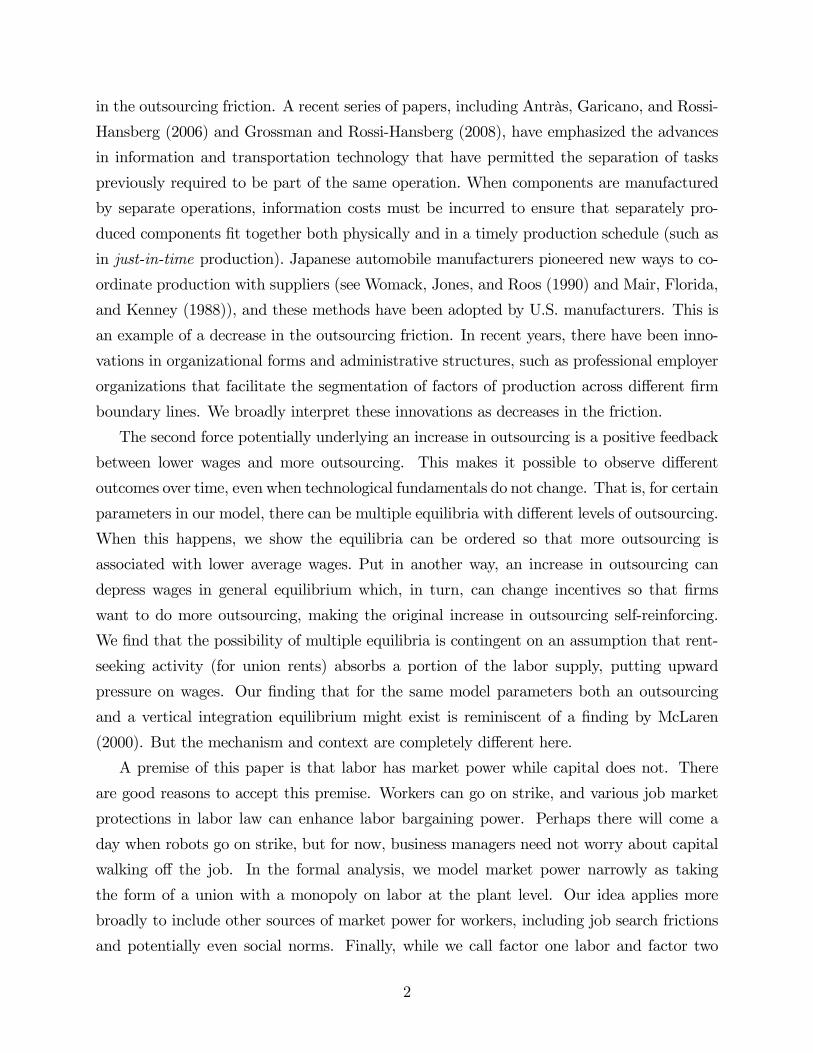
We assume that the existence of monopoly rents attracts resources, following a long

tradition in the economics literature. (See Posner (1975) for an early treatment and Cole

and Ohanian (2004) for a recent treatment.) That is, resources get dissipated through rent

seeking behavior. Specifically, of the units of labor that are inelastically supplied to the

economy, a portion goes toward rent seeking and the remaining portion ◦ goes to the

competitive spot market to work in production,

= + ◦.

We assume there is some matching process between the unit measure of firms and measure

of rent seekers that operates in a fashion such that the union rents in the economy

are divided equally (in expectation) across rent seekers. As an example matching process,

suppose for simplicity there are a finite number of firms and a finite number of rent seekers.

Begin by taking one firm and randomly draw a rent seeker from the pool of rent seekers

to which to assign the monopoly. Next, take a second firm and again randomly assign it to a

draw from the original pool of rent seekers. That is, use a “sampling with replacement”

process. With this process, any one rent seeker might end up with zero, one, or two or more

monopolies. Given our assumption of risk neutrality, the particulars of the distribution

across rent seekers will not matter, only the mean number of monopolies per rent seeker.

In summary, the abstraction employed here captures two main elements. First, there is

market power in the provision of the labor factor, but no analogous market power in the

provision of capital. In the formal setup, the rents go to the union and the production workers

receive the competitive wage. However, it is straightforward to reinterpret the structure so

that the people doing the production work are also engaging in rent seeking, so that the

actual wage received includes the competitive wage as well as a rent component. Second,

rent seeking consumes labor resources. This can be best understood as workers engaging in

search behavior to obtain union jobs. Finally, while we treat the rent-seeking assumption as

our baseline case, we also determine what happens without the rent-seeking assumption.

9

2.3 Timing and Equilibrium

Timing is in three stages. In stage 1, each firm commits to its vertical structure choice:

intermediate 1 specialist, intermediate 2 specialist, or fully integrated. Let be the share

of firms choosing vertical structure (with = 1 or = 2 for specialists and = for a

vertically integrated producer). Also in stage 1, a measure of workers choose to seek the

position of labor monopolist available at each firm. In stage 2, the labor monopolist at each

particular firm sets the wage for firm . In stage 3, inputs are procured and production

takes place.

An equilibrium is a list¡1 2

1 2 ◦ 1 2

¢that satisfies six con-

ditions. First, each firm’s choice of vertical structure ∈ {1 2 } must be optimal, takingas given how its choice impacts its wage and taking as given the output prices. Second,

the return to directing a unit of labor to the competitive spot market must equal the return

to rent seeking, that is,

◦ =

(7)

where the right-hand-side term averages the aggregate union rent over the labor units

that seek it. Third, the choice of wage offered by the union of a type firm must maximize

the union’s profit, given the anticipated demand behavior of the firm. Fourth, each firm of

type chooses inputs to maximize profits. Fifth, there must be market clearing in the spot

market for labor. Sixth, the intermediate prices 1 and 2 faced by specialist producers must

satisfy the arbitrage condition,

1 + 2 = (1− ) (8)

since combining one unit of each of the specialist produced goods yields 1− units of final

good.7

3 Results for a Fixed Open-Market Wage

We split the analysis of the model into two sections. In this section, we derive an initial

set of results on the workings of the model for a fixed open-market wage ◦. In the next

section, we take the open-market wage as endogenous and determine how it is impacted by

7Since we have assumed the supply of capital is perfectly elastic at , and since the rental rate is the

numeraire, = 1, the final good price in terms of the rental rate is an exogenous parameter.

10

outsourcing.

3.1 How Union Wages and Production Costs Vary with Vertical

Structure

It turns out that it is possible to derive optimal union wages without taking into account

equilibrium conditions in the output markets. This subsection derives the optimal union

wages and determines how production costs depend upon vertical structure.

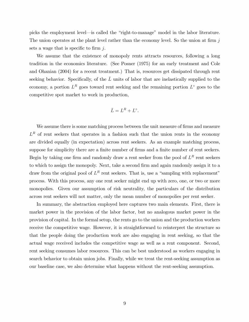
We begin with an analysis of an intermediate 1 specialist. Suppose we are at stage 3 and

an intermediate 1 specialist faces a wage of 1. To study the firm’s choice problem, it is

useful to first determine the cost function of constructing 1 units of the composite input.

Given the constant returns Cobb-Douglas production function (3), it is a standard result

that the cost function equals

1(1 1) = 11 1. (9)

(Since we are setting the rental rate on capital as the numeraire, = 1, the term 1− that

would normally appear drops out.) Furthermore, the cost-minimizing labor input choice is

1(1 1) = 1−(1−1)1 1. (10)

From (5), a specialist producer with composite input level 1 produces 1 units of inter-

mediate 1. Hence, profit at composite input 1 equals

1(1) = 11 − 1

1 1. (11)

Setting 1 to maximize profit yields the optimal choice of composite input 1

1 = (1)1

1− − 1−

1 . (12)

Plugging this into (10) yields the firm’s labor demand

1 () = 1 (1)1

1− −11 (13)

11

with constant elasticity

1 ≡ 1− (1− 1)

1− . (14)

A key point is that elasticity depends on the labor share coefficient 1. The higher 1, the

more elastic the labor demand.

With firm behavior at stage 3 pinned down, we go backward and examine the problem

of the labor monopolist in stage 2 picking 1. The labor monopolist obtains labor at the

open-market rate ◦ and posts a wage 1 to maximize the union rent

(1 − ◦) 1 ().

Note that the monopoly operates at the firm level, not the economy level. If the monopoly

were at the economy level, it would take into account the general equilibrium impact of the

posted wage. By operating at the firm level, the labor monopolist takes output prices and the

open-market wage ◦ as fixed. Since labor demand is constant elasticity, the rent-maximizing

wage satisfies the standard monopoly markup over marginal cost condition

1 =1

1− 11

◦ (15)

=1− (1− 1)

1◦. (16)

The analysis for an intermediate 2 specialist is the same as above with a change in

subscripts. Since 2 1, labor demand for an intermediate 2 firm is less elastic than for

an intermediate 1 firm, 2 1, and the wage is greater, 2 1.

We turn next to the case of a vertically integrated firm. Given the fixed coefficient tech-

nology for the final good, an integrated firm produces an equal amount of both intermediate

inputs. Let be the composite input level of each intermediate. Given , the cost of

producing both intermediates at this level is

( ) = 1 + 2 = (1 + 2) . (17)

Using the production function of the vertically integrated firm given by (6), we can write

profit as

= 2−(1−) − (1 + 2) . (18)

12

From (10), the firm’s labor demand added up over both intermediate goods equals

= 1−(1−1) + 2

−(1−2) (19)

Maximizing (18) with respect to the choice of and then plugging into (19) yields the

labor demand function faced by the union,

() =¡2

−(1−)¢ 11−¡1

−(1−1) + 2−(1−2)¢ (1 + 2)

− 11− (20)

The union picks to maximize

( − ◦) ()

Let solve this problem. In general, no analytic solution exists. However, we can obtain

an expression for the limiting case where 1 goes to 1 and 2 goes to zero,

lim1→1

=1− + ◦

.

By way of comparison, the wages set to specialist firms from (15) at this limit are

lim1→1

1 =◦

(21)

lim1→1

2 = ∞.

This follows because the elasticity for a specialist producing intermediate 1 goes to 11− while

it goes to 1 for intermediate 2.

A key result that plays an important role in the subsequent analysis is that the total

cost of constructing a composite input for each intermediate is less under specialization than

under vertical integration. Let and be the cost of producing one unit of composite

input in the vertically integrated and specialist cases. Note that if 1 = 2 =12, the two

intermediates are the same in elasticity, and there is no difference between the specialization

structure and vertical integration in terms of union wage setting behavior; i.e., = .

But when 1 12, there is a difference. We begin with an analytic result at the limit where

1 goes to one. Let = 1 + 2 be the combined cost to the vertically integrated firm

of one unit of each composite input.

13

Lemma 1.

lim1→1

[1 + 2] lim1→1

Proof. In the appendix we show that

lim1→1

1 =◦

lim1→1

2 = 1

lim1→1

=1 + ◦

which immediately implies the result. ¥One thing to note about the limit for an intermediate 2 specialist is that even though

the wage is going to infinity, the spending share on labor is going to zero. In the limit, the

intermediate 2 specialist needs only to worry about expenditures on capital. At the limit,

it requires one unit of capital to make one composite input. Since = 1, it follows that

lim1→1 2 = 1.

Understanding the limit where intermediate 1 is pure labor and intermediate 2 pure cap-

ital is easy. The demand for labor by a vertically integrated firm, for which labor represents

only part of the factor bill, is obviously less elastic than for an intermediate 1 specialist, for

which labor is the only input. So the union sets a higher wage to an integrated plant. By

outsourcing the labor task, there is a clear savings in the wage bill, while the task using

capital pays the market rate for capital either way.

Things are more subtle in the general case, 1 1, 2 0, where both intermediates

use both factors. Here, there is a trade-off. By splitting up production, an intermediate

1 specialist pays a lower wage compared to an integrated plant. But an intermediate 2

specialist pays a higher wage. Intuitively, since the former uses labor intensively while the

latter does not, the cost savings on the former should outweigh the cost increases on the

latter. We can show with numerical methods that this is true.8 By scanning over a fine grid

of 1 ∈ (12 1), ∈ (0 1), and ◦ (and 2 = 1− 1), we find that

[1 + 2] . (22)

8We verify this claim over a fine grid across the ranges 1 ∈ [51 99], ∈ [03 99], and ◦ ∈ [01 500]We stay away from extreme values to avoid numerical inaccuracies.

14

3.2 Choice of Vertical Structure

In this subsection we examine a firm’s choice of vertical structure. For a fixed open-market

wage ◦, we determine how the vertical structure choice depends on the outsourcing friction

.

Proposition 1. For any open-market wage ◦, there exists a unique (◦) 0, such that

if (◦), all firms are specialized while if (◦), all firms are vertically integrated.

Proof. Given an output price and a unit composite input cost of an intermediate

specialist, it is straightforward to derive its maximized profit,

=h

1− −

11−i

11− ()

− 1− . (23)

Analogously, using (18), the profit of a vertically integrated union firm equals

=1

2

h

1− −

11−i

11− ( )

− 1− (24)

If there is an equilibrium with specialization, both intermediate goods must be produced,

and so firms must be indifferent between producing both, i.e., 1 = 2. By arbitrage, we

also have 1 + 2 = (1− ) . Using these two equations, we can solve out for 1 as

1 =(2)

−

(1)−+ (2)

− (1− ) . (25)

Plugging this into (23) and using straightforward algebra, a firm prefers specialization to

integration if and only if

(2)−(1)

−

(1)−+ (2)

− (1− )

µ1

2

¶1−( )

−. (26)

Recall from the previous section that 1 + 2 . Lemma A1 in the appendix shows

that when 1 + 2 holds, (26) holds at = 0. Define to be the unique where

(26) holds with equality. ¥That outsourcing does not take place when is large is obvious. What is interesting about

Proposition 1 is that outsourcing necessarily does take place when the friction is small but

still positive. Recall that, in this environment, vertical structure would be indeterminate

15

if both factor markets were competitive and if the friction were zero. If factor markets

were competitive and there were any positive friction, integration would necessarily prevail,

as there is no technological benefit from specialization. But with monopoly in the labor

market, there is an incentive to vertically disintegrate to limit rent extraction by the unions.

So specialization prevails if the outsourcing friction is small enough.

The shape of the relationship between the cutoff and the open-market wage ◦ plays

a role in the subsequent analysis. We call this the “ curve” and we plot it in Figure 1

for several different values of 1, 1 ∈ {06 08 1}, fixing = 05.9 We put the wage ◦

on the vertical axis and on the horizontal, because this will be convenient later when

is exogenous and ◦ is endogenous. As illustrated, for a given value of 1, there exists a

◦min such that (◦) strictly decreases in ◦ for ◦ ◦min, and strictly increases in ◦

for ◦ ◦min. We can prove analytically that this property holds at 1 = 1, and we verify

numerically that the property holds for general 1.10 Note that in the opposite limiting case

of 1 = 2 =12, vertical structure has no impact on wages, since both intermediates have

the same labor intensity. In this extreme case, (◦) = 0 for all ◦. So the case of high 1

is the interesting case.

4 Outsourcing and Wage Decline

We now solve for equilibrium in the labor market and determine how both the open-market

wage ◦ and the level of union rents vary with the outsourcing friction .

It is convenient to split up the analysis. First, we impose an artificial restriction that

vertical integration is infeasible so all firms must be specialists and determine what the

equilibrium would look like in this case. Next, we flip the restriction so only integration is

feasible. In the end, we allow both to be feasible and determine what happens.

4.1 Only Specialization

This subsection determines equilibrium when integration is not an option. We solve for how

the demand for labor depends upon a given ◦ and then solve for market clearing.

Given ◦ and the associated union markups over ◦ (see (15)), let 1(◦) and 2(◦)

9We fix = 5 to construct all the figures. Also, the wage on the vertical axis is in log scale.10The analytic proof for the 1 = 1 case is available in separate notes. Our numerical result for 1 1

uses the same grid as in footnote 8.

16

be the prices that equate the profit of an intermediate 1 specialist with an intermediate 2

specialist (see (25)) and that solve the arbitrage condition 1+2 = (1− ) . Let (◦) be

the derived demand for labor for specialist taking into account the impact of ◦ on price.

That is, using (13),

(◦) = ((

◦))1

1− 1(◦)−.

Analogously, let (◦) be the derived supply of intermediate by a specialist . Let (◦) be

the share of firms producing intermediate consistent with market clearing of intermediates,

i.e.,

1(◦)1(

◦) = 2(◦)2(

◦),

since the left and right sides are the total productions of intermediates 1 and 2 and these

must be equalized because of fixed coefficients. Using 1 = 1− 2, we have

1(◦) =

2(◦)

1(◦) + 2(◦).

Putting all of this together, the total demand in the economy for production labor at an

open-market wage ◦ across the two kinds of intermediates equals

◦(◦) =

2X=1

(◦)(

◦),

where the subscript signifies we are in the Only Specialization case.

We turn now to the labor allocated to rent seeking. When the open-market wage is ◦,

total union rents are

(◦) =

2X=1

[(◦)− ◦] (

◦)(◦).

Plugging this into the equilibrium condition (7) that equalizes the return to rent seeking and

◦, we can solve for the demand for rent-seeking labor,

(

◦) =(

◦)◦

.

Adding this to the demand for production labor yields the overall demand for labor in the

economy,

(

◦ ) = ◦(◦ ) +

(◦ ), (27)

17

where we note the explicit dependence of demand on the outsourcing friction, as this is useful

at this point. Market clearing requires that demand (

◦ ) equal the exogenous supply

. We obtain the following result for the limiting case.

Lemma 2. Assume the limiting case of 1 = 1 and 2 = 0. (i) Overall demand (

◦ )

strictly decreases in ◦ and . (ii) For a given , there exists a unique ◦∗ () that clears the

open market, (

◦∗ () ) ≡ and ◦∗ () is strictly decreasing in . (iii) A single-crossing

property holds between the ◦∗ curve and the curve defined earlier. Formally, for any 0

where 0 (◦∗ (0)), then (◦∗ ()) for all 0.

Proof. See appendix.¥We use numerical methods to verify that the three properties listed hold for general 1.

11

The relationship ◦∗ () is what the equilibrium open-market wage would be if special-

ization were the only feasible vertical structure. We call this the “◦∗ curve” and illustrate

it in Figure 2 for two cases: one where labor supply is small, so ◦∗ is high, and the other

where is large, so ◦∗ is low. The figure illustrates that ◦∗ strictly decreases in (part

(ii) of the lemma). Moreover, it crosses the curve only once (part (iii)). Let + be defined

as the where the intersection occurs,

≡ (

−1(+ ) + ). (28)

4.2 Only Integration

Now consider the case where only vertical integration is feasible. Analogous to (27) above, we

can construct labor demand (

◦ ) and equate this to supply to obtain the equilibrium

open-market wage ◦∗ (). We can show the analog of Lemma 2 holds for this case, with one

difference.12 In the integration case, the outsourcing friction is irrelevant, so ◦∗ () and

(

◦ ) are constant as functions of . (This makes the single crossing property trivial

in the integration case.) Figure 3 illustrates two example ◦∗ curves: one with small and

the other with large. Analogous to (28), define + to be the point where ◦∗ intersects

.

11We verify (i) holds over a grid across the ranges 1 ∈ [55 9], = [1 9], ∈ [5 10], ◦ ∈ [2 100] and ∈ [0 95]. For (ii) and (iii), we consider ∈ [1 5] and narrow the range of to ∈ [0 6] to maintainnumerical accuracy.12Beyond analytic results for the 1 = 1 case, we also confirm that the analog of Lemma 2 holds for general

1 ∈¡12 1¢. Parts (ii) and (iii) are analytically straightforward. We verify part (i) (that (

◦ ) isstrictly decreasing in ◦) numerically using the same grid as in footnote 11.

18

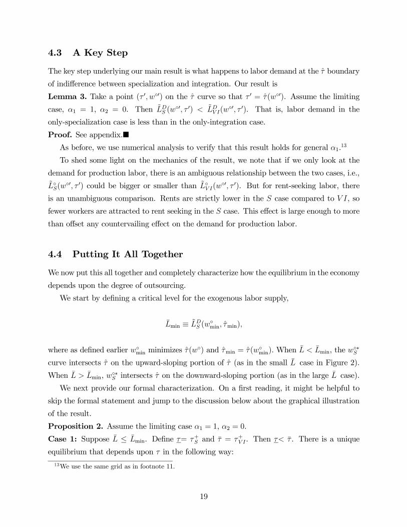
4.3 A Key Step

The key step underlying our main result is what happens to labor demand at the boundary

of indifference between specialization and integration. Our result is

Lemma 3. Take a point ( 0 ◦0) on the curve so that 0 = (◦0). Assume the limiting

case, 1 = 1, 2 = 0. Then (

◦0 0) (

◦0 0). That is, labor demand in the

only-specialization case is less than in the only-integration case.

Proof. See appendix.¥As before, we use numerical analysis to verify that this result holds for general 1.

13

To shed some light on the mechanics of the result, we note that if we only look at the

demand for production labor, there is an ambiguous relationship between the two cases, i.e.,

◦(◦0 0) could be bigger or smaller than ◦ (

◦0 0). But for rent-seeking labor, there

is an unambiguous comparison. Rents are strictly lower in the case compared to , so

fewer workers are attracted to rent seeking in the case. This effect is large enough to more

than offset any countervailing effect on the demand for production labor.

4.4 Putting It All Together

We now put this all together and completely characterize how the equilibrium in the economy

depends upon the degree of outsourcing.

We start by defining a critical level for the exogenous labor supply,

min ≡ (

◦min min)

where as defined earlier ◦min minimizes (◦) and min = (◦min). When min, the

◦∗

curve intersects on the upward-sloping portion of (as in the small case in Figure 2).

When min, ◦∗ intersects on the downward-sloping portion (as in the large case).

We next provide our formal characterization. On a first reading, it might be helpful to

skip the formal statement and jump to the discussion below about the graphical illustration

of the result.

Proposition 2. Assume the limiting case 1 = 1, 2 = 0.

Case 1: Suppose ≤ min. Define = + and = + . Then . There is a unique

equilibrium that depends upon in the following way:

13We use the same grid as in footnote 11.

19

Subcase 1(i) For , no firms are integrated, i.e., = 0, and the equilibrium open-

market wage is

◦∗() = ◦∗ ().

Subcase 1(ii) For , all firms are vertically integrated, = 1, and the equilibrium

open-market wage is

◦∗() = ◦∗ ().

Subcase 1(iii) For ∈ ( ), there is partial integration, 0 1. The wage is

determined from the curve,

◦∗() = −1().

The share of firms that are vertically integrated is the unique satisfying

(

−1() ) + (1− ) (

−1() ) =

and strictly increases in . Also, the equilibrium wage ◦∗() strictly increases in , so

more outsourcing co-moves with lower wages.

Case 2: Suppose min. If ◦∗ ≤ ◦min (meaning

+ is on the downward-sloping portion

of the curve as illustrated in the large- case in Figure 4), then define ≡ + and ≡ + .

If ◦∗ ◦min, then define ≡ min and ≡ + . Note .

For and max© +

ª, there is a unique equilibrium that follows the pattern

of Subcases 1(i) and 1(ii) above. If + and ∈ ( + ), there is a unique equilibriumwith partial integration following Subcase 1(iii) above.

For ∈ ( ), a nonempty open interval, there are three equilibria labeled and

. Equilibrium has full specialization, = 0. Equilibria has partial integration,

∈ (0 1). Equilibrium has partial or full integration, ∈ (0 1], and . Across

the three equilibria, there is a strict ordering that less integration is associated with a lower

open-market wage, ◦ ◦ ◦.

Proof. See appendix.¥The result is best understood with a graph. Figure 4 combines Figure 2 (keeping the ◦∗

to the left of because specialization is preferred there) with Figure 3 (keeping ◦∗ to the

right of because integration is preferred there). Consider first the small- case on the top

portion of Figure 4. The set of ( ◦) pairs that are equilibria are highlighted by the solid

dark line. Notice point where the ◦∗ curve intersects the curve. There is an equilibrium

20

here where all firms are specialized because (1) being on the curve means firms are just as

happy to be specialized as integrated and (2) being on the ◦∗ curve means supply equals

demand in the labor market. For to the left of point , complete specialization is the only

possibility, and we follow along the ◦∗ curve to pin down the wage. Notice that as is

decreased in this range, wages rise. This is an example of the productivity effect highlighted

in Grossman and Rossi-Hansberg (2008). Over this region, all activity is outsourced, and

the impact of reducing the friction is that this given level of outsourcing takes place more

efficiently. Some of the gain is passed along in terms of higher wages.

Next, notice point where ◦∗ intersects the curve. Observe point is at a higher

wage than . This necessarily follows from Lemma 3. At point , if firms were to switch

over to vertical integration from specialization (which they are indifferent to doing), total

labor demand would increase. To get market clearing, the wage needs to increase, and that

is what happens at point B. For in between points and , the wage is set on the curve

to make firms indifferent to vertical structure. A fraction are integrated, and this share

is chosen to clear the labor market. The key thing to note is that as we move from to

and lower the outsourcing friction, the extent of outsourcing increases at the same time that

the wage falls. This is the main result of the paper.

Next, consider the large case illustrated at the bottom of Figure 4 where the action

is on the downward-sloping portion of the curve. Again, the equilibria are highlighted by

a solid dark line. Consider what happens for between points and . For any such ,

we see there are three equilibria: (1) a pure specialization equilibrium ( = 0) on the ◦∗

curve with a low wage, (2) a pure integration equilibrium ( = 1) on the ◦∗ curve with a

high wage, and (3) a partial integration equilibrium with an intermediate wage. Again, an

increase in outsourcing goes together with a decline in wages. But this time we are moving

across equilibria with no change in economic fundamentals (i.e., is fixed).

We have been focusing on the open-market wage, but we now turn to the average wage

paid by firms. This is the wage bill added up across all firms divided by the number of

production workers. It equals

=111 + 222 +

11 + 22 +

=◦◦ +

◦= ◦ +

◦,

which is the open-market wage plus the average union markup. Above we show that the

21

open-market wage declines with outsourcing. Our next result shows that the mean firm wage

also declines with outsourcing.

Proposition 3. Suppose 1 = 1, 2 = 0.

(i) Assume Case 1 where ≤ min so there is a unique equilibrium. In the region of

partial integration, ∈ ( ), the mean firm wage is lower the lower is .

(ii) Assume Case 2 where min so there is a range of ∈ ( ) with multipleequilibria. Across the multiple equilibria, less integration is associated with a lower mean

firm wage.

Sketch of Proof. Calculations in the appendix show that ◦ decreases with outsourcing.

Since ◦ goes down, both effects work together to lower the mean firm wage.¥

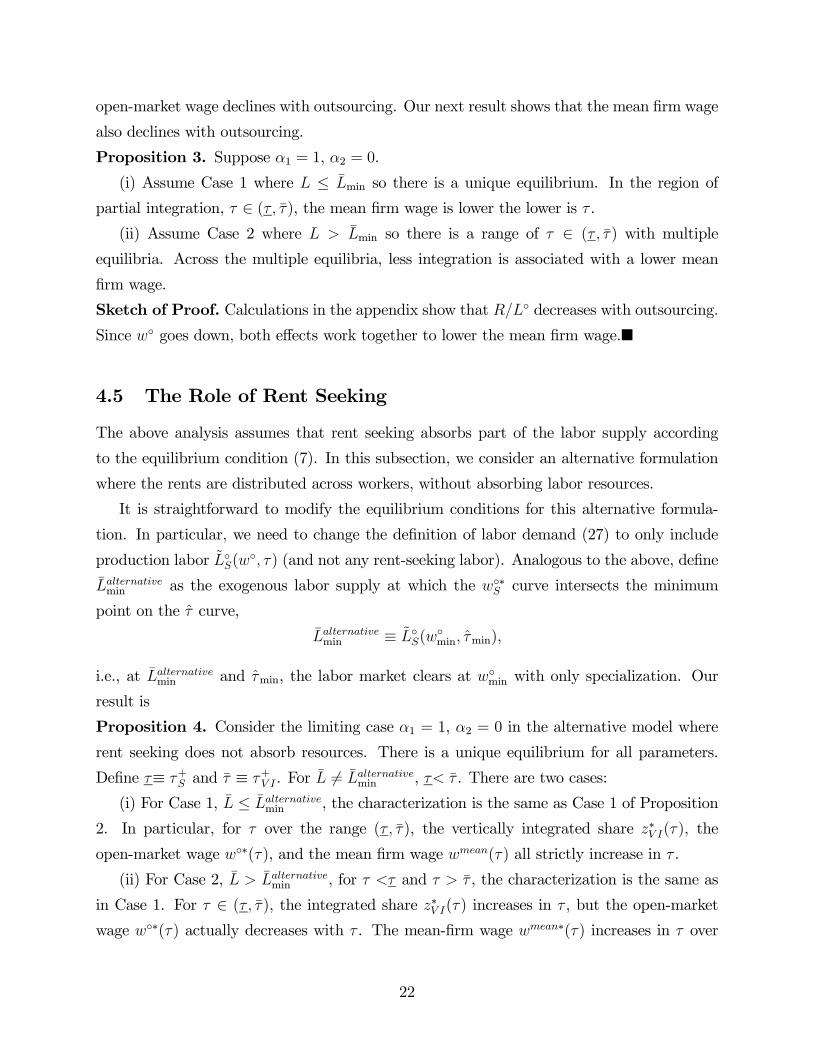
4.5 The Role of Rent Seeking

The above analysis assumes that rent seeking absorbs part of the labor supply according

to the equilibrium condition (7). In this subsection, we consider an alternative formulation

where the rents are distributed across workers, without absorbing labor resources.

It is straightforward to modify the equilibrium conditions for this alternative formula-

tion. In particular, we need to change the definition of labor demand (27) to only include

production labor ◦(◦ ) (and not any rent-seeking labor). Analogous to the above, define

min as the exogenous labor supply at which the ◦∗ curve intersects the minimum

point on the curve,

min ≡ ◦(

◦min min),

i.e., at min and min, the labor market clears at

◦min with only specialization. Our

result is

Proposition 4. Consider the limiting case 1 = 1, 2 = 0 in the alternative model where

rent seeking does not absorb resources. There is a unique equilibrium for all parameters.

Define ≡ + and ≡ + . For 6= min , . There are two cases:

(i) For Case 1, ≤ min , the characterization is the same as Case 1 of Proposition

2. In particular, for over the range ( ), the vertically integrated share ∗ (), the

open-market wage ◦∗(), and the mean firm wage () all strictly increase in .

(ii) For Case 2, min , for and , the characterization is the same as

in Case 1. For ∈ ( ), the integrated share ∗ () increases in , but the open-market

wage ◦∗() actually decreases with . The mean-firm wage ∗() increases in over

22

this range.

Proof. The appendix sketches the proof. We emphasize that the final claim that ∗()

increases in in Case 2 and ∈ ( ) is based on numerical analysis. The calculationinvolves a nonlinear equation that is difficult to characterize analytically.¥When is low so that the ◦∗ intersects on the upward-sloping portion, the analysis

in the alternative model is identical to the baseline. But things are different when the

intersection occurs on the downward-sloping portion, as illustrated in Figure 5. Here, the

result in Lemma 3 flips sign, so that the ◦∗ curve actually cuts the curve below where

it intersects ◦∗ , as illustrated. Readily apparent from the figure is that the equilibrium

is unique for each ; the region of multiplicity in Figure 4 is gone. Note the equilibrium

open-market wage ◦∗ actually decreases in from point to point , so in this way the

analysis is different from the baseline. But the mean wage paid by firms is the relevant

wage measure to be looking at. This increases with from point to point , analogous

to Proposition 3. So our main result from the baseline model that increases in outsourcing

go together with declines in wages is preserved in the alternative model.

It is interesting that there are no multiple equilibria in the alternative model. To get

a sense of what is different here, observe first that the emergence of outsourcing depresses

labor rents. In the baseline model, the reduction in rents attracts less labor to outsourcing,

leaving more labor for production and further depressing wages. It is possible for these lower

wages to spur additional outsourcing, creating a positive feedback loop and reinforcing the

original outsourcing at the start of the story. When the rent-seeking element is taken out, a

piece of the loop is gone, and the equilibrium is now unique.

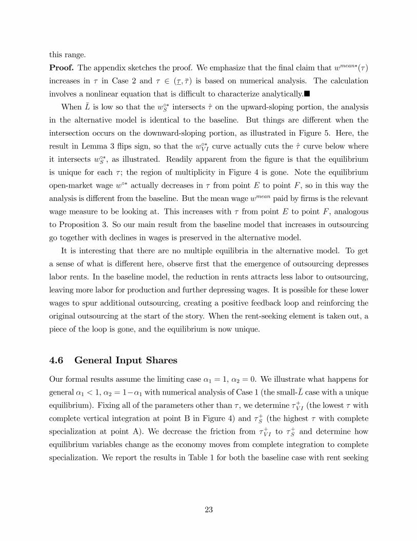
4.6 General Input Shares

Our formal results assume the limiting case 1 = 1, 2 = 0. We illustrate what happens for

general 1 1, 2 = 1−1 with numerical analysis of Case 1 (the small- case with a uniqueequilibrium). Fixing all of the parameters other than , we determine + (the lowest with

complete vertical integration at point B in Figure 4) and + (the highest with complete

specialization at point A). We decrease the friction from + to + and determine how

equilibrium variables change as the economy moves from complete integration to complete

specialization. We report the results in Table 1 for both the baseline case with rent seeking

23

and the non-rent-seeking case.14

Panel A reports the limiting case of 1 = 1 that is covered in Propositions 3 and 4.

We know from these results that ◦ and both decrease as decreases from + to

+ , and we can see this in the table. Note that wages are significantly higher in the rent-

seeking case because rent seeking absorbs labor driving up wages. We also report the total

wage bill, total firm profits, and total surplus (the sum of firm profits plus the wage bill).

In terms of effects on total surplus, there are three considerations. First, the switch from

integration to outsourcing weakens the labor monopoly, which reduces wasteful rent-seeking

behavior. Second, firms’ decisions are less distorted. Offsetting these positive impacts is a

third consideration that outsourcing entails a friction (approximately 13 percent of output

in Panel A) that is avoided with integration. In the rent-seeking case, the net effect of

outsourcing on surplus is strictly positive.15 With no rent seeking, the first consideration is

eliminated, and the net effect on total surplus is negative; the cost of the friction outweighs

the benefits of reduced distortions. Despite the friction, firms outsource because profits are

higher.

The remaining panels in Table 1 report the results for values of 1 below one. The

qualitative results are identical to what we get for the 1 = 1 case in Panel A. Quantitatively,

as 1 is decreased toward its lower bound of12, the effects become smaller and go to zero.

At this lower bound, there is no difference in factor intensity between the two intermediates

and the incentive for outsourcing disappears ( goes to zero). One interesting thing in these

remaining panels is what happens to the wage bill for intermediate 2, the capital-intensive

task. This is positive in the remaining panels, since 2 0. Note that this wage bill strictly

increases with outsourcing throughout all the cases. So from labor’s perspective, the process

of vertical disintegration has offsetting effects: the wage bill for intermediate 2 goes up, the

wage bill for intermediate 1 goes down. The key finding of the paper is that the combined

impact is negative.

5 Concluding Remarks

We have developed a new general equilibrium model of outsourcing and have put it to

work analyzing the connection between outsourcing and wages. We believe this structure

14Throughout the table, = 5 and = 16 are held fixed. We have rescaled the total wage bill, profits,

and total surplus by multiplying through by 100.15The net positive impact is negligible for 1 = 1 but is significant in the other cases.

24

is potentially useful for examining other issues related to outsourcing. For example, in our

analysis, firms are identical in the extent to which they face a union monopoly. A natural

extension is to allow firms to differ in this dimension. We have done some preliminary

analysis of what happens when some firms are union and others nonunion and can show

that if nonunion firms ever specialize, they do the labor-intensive task. We could use the

structure to look at how changes in the extent of unionism impact the degree of outsourcing

and also how outsourcing feeds back and impacts the incentive to organize unions. As another

application, we can put this structure in an international context, and study how exposure

to international trade impacts the incentive for domestic outsourcing. We expect interesting

effects to emerge here because wages impact the incentive for domestic outsourcing (Figure

1) and trade impacts wages.

25

Appendix

A.1 Background Calculations for Section 3We begin by deriving the integrated firm’s labor demand. The cost function can be

written as

( ) = 1 + 2 = (1 + 2) (29)

= .

Now if the firm produces of each input, it obtains final good production of

= (2)−(1−)

(30)

= 2−(1−). (31)

So the firm’s problem is

max 2−(1−) − .

The FONC is

2−(1−)−1 − = 0.

Or

=¡2

−(1−)¢ 11−

− 11−

. (32)

We can plug this into the firm’s labor demand to obtain the demand faced by the labor

union:

() = 1−(1−1) + 2

−(1−2)

=¡1

−(1−1) + 2−(1−2)¢ ¡2−(1−)¢ 1

1− − 11−

=¡2

−(1−)¢ 11−¡1

−(1−1) + 2−(1−2)¢ (1 + 2)

− 11−

= ¡1

−(1−1) + 2−(1−2)¢ (1 + 2)

− 11− .

We use (29) to substitute in for in the third line. The term in the fourth line is a

multiplicative constant independent of .

26

Thus, the labor union facing a vertically integrated firm sets to maximize:

( − ◦)¡1

−(1−1) + 2−(1−2)¢ (1 + 2)

− 11− . (33)

Straightforward manipulations of the FONC of problem (33) yields

0 = 1− (1− ) ( − ◦)(−(1−) + −)

( + (1− )1−)

−µ

1

1−

¶( − ◦)

¡−(1−) + (1− )−

¢ + (1−)

,

where to simplify notation, we set 1 = and 2 = 1− . In the limiting case of = 1, we

can solve for the optimal union wage as

lim→1

=1− + ◦

.

We next look at costs at the limit under specialization. Using 2 = 1− , and equation

(15) for the optimal union wage, we can solve for the limiting cost of an intermediate 2

specialist as

lim→1

2 = lim→1

£1−2

¤= lim

→1

∙1−

(1− ) ◦¸1−

= 1,

where the last line follows from straightforward limit analysis. For an intermediate 1 spe-

cialist, using (21), we have

lim→1

1 = 1 =

◦

.

Next we prove Lemma A1 used in Proposition 1.

Lemma A1. Suppose for 0, 0 there is a ≥ + . Then

−−

− + −

µ1

2

¶1−−.

27

Proof. We can rescale things so that + = 1 and show the results holds for = 1.

Equivalently, that

− (1− )−

− + (1− )−

µ1

2

¶1−. (34)

Define () by

() ≡ 2− (1− )− − 2− − 2 (1− )

−.

Straightforward manipulation of (34) shows that it holds if () 0 for ∈ [0 12). Now it

is easy to verify that (12) = 0. So it is sufficient to show that 0() 0 for ∈ [0 1

2). We

prove this in separate notes. ¥Finally, we prove the claims made in Section 3 about the shape of the function in the

limit where 1 = 1, 2 = 0. From (26), we can write as

= 1−µ1

2

1−−

¶ ¡−1 +

−2

¢−1

−2

.

Substituting in the limiting values for , 1 and 2 from above, we have

(◦) = 1− 12

1− µ1 + ◦

¶− µ1 +

µ◦

¶¶.

Straightforward differentiation shows that the minimum of this function is obtained at a

level

◦min ≡ − 1− (35)

and that (◦) is strictly decreasing or increasing as ◦ ◦min or ◦ ◦min.

A.2 Proofs of Results in Section 4Lemma 2. Assume the limiting case of 1 = 1 and 2 = 0. (i) Overall demand

(◦ )

strictly decreases in ◦ and . (ii) For a given , there exists a unique ◦∗ () that clears

the open market, (

◦∗ () ) ≡ and ◦∗ () is strictly decreasing in . (iii) For any 0

where 0 (◦∗ (0)), then (◦∗ ()) for all 0.

Proof.

28

We begin by calculating the production labor demand ◦(◦ ). In the limit where

1 = 1 and 2 = 0, prices equal

1 =1

◦− + 1(1− ) (36)

2 =◦−

◦− + 1(1− ) ,

where we use (25) and we substitute in 1 and 2 from above. Now in the limit, labor

demand simply equals composite input, 1 = 1. Using formula (12) for the optimal choice

of 1 and substituting in the optimal union wage 1 = ◦ at the limit, we have

1 =

µ1

2

◦

¶ 11−

(37)

for 1 given above.

Next we determine the share of firms 1 choosing to be intermediate 1 specialists. From

above2

1= ◦−.

Using the optimal choice of from (12), we have

2

1=(22)

11−

(11)1

1−=

1−

◦− 1−

µ◦

¶ 11−

=◦

.

Since = ,

2

1=

µ◦

¶

.

Now given fixed proportions,

11 = 22 = (1− 1) 2.

Thus

1 =1

1 + 12

=1

1 + ◦−. (38)

29

Combining (36), (37), and (38) yields

◦(◦ ) = 11 =

∙1

1 + ◦−

¸ 2−1−µ1

◦

¶ 11− ¡

(1− ) 2¢ 11− . (39)

The union rent is

(◦ ) = (1 − ◦) 11 =

1−

◦◦(

◦ ).

Total labor demand equals

(

◦ ) = ◦(◦ ) +

(◦ ) (40)

= ◦(◦ ) +

(◦ )

◦

= ◦(◦ ) +

(1 − ◦) ◦(◦ )

◦

=1

◦(

◦ ).

Thus total demand (

◦ ) is proportional to production work demand ◦(◦ ). It is

immediate that ◦ strictly decreases in . Straightforward calculations in separate notes

show ◦ strictly decreases in ◦. Claims (i) and (ii) then follow. To prove (iii), suppose we

have a , and define ◦ ≡ ◦∗(), ◦ ≡ ◦∗( ), where ◦ ◦ from (ii). Suppose

that = (◦), i.e.

1− =1

2

1− µ1 + ◦

¶− µ1 +

µ◦

¶¶. (41)

We need to show (◦ ), or

1− 1

2

1− µ1 + ◦

¶− µ1 +

µ◦

¶¶(42)

30

Now by definition of market clearing = ◦(◦ ) = ◦(

◦ ). Taking the formula

(39) for ◦ to the (1− ) power and canceling terms yields

∙1

1 + ◦−

¸(2−)µ1

◦

¶(1− ) (43)

=

∙1

1 + ◦−

¸(2−)µ1

◦

¶(1− ) .

Dividing both sides of (42) by (1− ) and using (43) to substitute in for (1− ) (1− )

on the left-hand side and (41) to substitute in for (1− ) on the right-hand side, it follows

that we need to show

◦£1 + (◦ )

−¤2−◦£1 + (◦)

−¤2−

³1+

´− ³1 +

³

´´³1+

´− ³1 +

³

´´ ,or equivalently, that

◦£1 + (◦)

−¤2−◦£1 + (◦ )

−¤2−

³1+

´− ³1 +

³

´´³1+

´− ³1 +

³

´´ .Since ◦ ◦ , it is sufficient to show

(◦) ≡

³1 +

³◦

´´£1 + (◦)−

¤2− µ 1

◦

¶µ1 + ◦

¶−

=

³1+◦

´−−£

◦ + (◦)1−¤1−

is strictly decreasing in ◦ which is immediate. This proves (iii). ¥As background for the proof of the next Lemma, we derive demand and rents for the

only-integration case in the limiting case. Using (32), that =1+◦, that = in the

limiting case, and that ◦ = since = 1, production labor demand equals

◦ (◦ ) =

1

2

µ

2

1 + ◦

¶ 11−

(44)

31

Total labor demand equals

(

◦ ) = ◦ (◦ ) +

(◦ ) = ◦ (

◦ ) + (

◦ )◦

(45)

= ◦ (◦ ) +

1

◦

µ1− + ◦

− ◦

¶◦ (

◦ )

=

µ1− + ◦

◦

¶◦ (

◦ ).

This is strictly decreasing in ◦, so ◦∗ () solving = (

◦ ) is unique. Since

◦ (◦ ) does not depend on , it follows that ◦∗ () is independent of .

Lemma 3. Take a point ( 0 ◦0) on the curve so that 0 = (◦0). Assume the limiting

case, 1 = 1, 2 = 0. Then (

◦0 0) (

◦0 0). That is, labor demand in the

only-specialization case is less than in the only-integration case.

Proof. Using the formulas (37) for 1 and (44) for (and keeping in mind that ◦ =

since = 1), we have

1

=

³1

2

◦

´ 11−

12

³2

1+◦

´ 11−.

On the curve, 1 = . Hence, using (23) and (24), and substituting in 1 = ◦,

= (1 + ◦) , we have

1

1−1

µ◦

¶− 1−

=1

2

11−

µ1 + ◦

¶− 1−.

Therefore,1

=1 + ◦

◦.

Recalling that =

1◦, that

◦ = 11, substituting in for 1 from (38) and using ◦ =

, it follows that

=

1

11 =

1

11 + ◦

◦◦ (46)

=1

1

1 + ◦−1 + ◦

◦◦ .

32

Using (45) above,

if and only if

1

1

1 + ◦−1 + ◦

◦1− + ◦

◦

or

(1 + ◦) (1− + ◦)¡1 + ◦−

¢.

We use straightforward calculations to show this is true for ◦ 0 in separate notes. ¥Proof of Proposition 2

Case 1. Since = + and = + in the statement of the proposition, Lemma 3 immediately

implies . It is immediate that the equilibrium has to be on the ◦∗ curve for , the

curve for ∈ ( ), and the ◦∗ curve, as claimed. The only thing left to prove for Case1 is that for ∈ ( ), there exists a unique defined by

(

−1() ) + (1− ) (

−1() ) = (47)

that strictly increases in .

Note that by the definition of + , for + = (

−1() ) , analogously, for

+ = , (

−1() ) . Hence for ∈ ( ), a unique ∈ (0 1) solves theequation (47) as claimed. For a given 0 ∈ ( ), let 0 be the share solving (47). Considera higher 00 0, but still 00 . We note first that

0 (

−1( 00) 00) + (1− 0 ) (

−1( 00) 00) ,

i.e. holding the share fixed, but increasing along that curve, lowers demand. To

show this, note that with Case 1 we are on the upward-sloping portion of the curve

so −1( 00) −1( 0). Since decreases in ◦ and , and since

decreases in ,

(

−1( 00) 00) (

−1( 0) ) and (

−1( 00) 00) (

−1( 0) 0), proving the above

inequality. Hence the the equilibrium share 00 for 00 must satisfy 00 0 .

Case 2.

For outside the interval ( + ), the arguments are the same as Case 1.

Given min, the point defined in the statement of the proposition satisfies + .

For all ∈ ( + ), all the points on the ◦∗ curve are to the left of the curve, (◦∗ ()).

For all these points, firms strictly prefer specialization over integration and we have labor-

33

market clearing, so each pair ( ◦∗ ()) is equilibrium with = 0. This is the type

equilibrium.

To construct the other two equilibria, we need to consider three different subcases.

The first subcase is ◦∗ ≤ ◦min. Then + ∈ [min + ) and ◦∗ () ◦min, for ∈( + ). Note that for all such , all the points on ◦∗ are to the right of the curve,

(◦∗ ), so firms strictly prefer vertical integration. The points in this region are

type equilibria, with = 1. Next, for this range of define ◦ = −1(), where

◦∗ () ◦ ◦∗ . Letting solve (47), this is a partial integration equilibrium. That

◦ ◦ ◦ is immediate.

Next suppose ◦∗ ◦min, but + + . For ∈ (+ + ), the and equilibria are

constructed the same in the first subcase. For ∈ (min + ), there are two points on the curve between ◦∗ and ◦∗ . Formally, for such there exists a ◦ and a ◦ such that

= (◦) = (◦) and ◦∗ () ◦ ◦ ◦∗ . Pick and to satisfy (47).

Finally suppose ◦∗ ◦min but + ≥ + . Then for ∈ (min + ) there are two partial

equilibria analogous to that described in the previous case. For + , we are back to the

case of a unique equilibrium.¥

Proof of Proposition 3.

Using (7), we can write rents divided by production workers as:

◦= ◦

◦

= ◦

+ (1− )

◦ + (1− )

◦

.

Note that in constructing the equilibrium, we are taking a convex combination of the equilib-

ria of the only-specialization and only-integration regimes. For each extreme case the return

to rent-seeking is ◦ and so this is also the return to rent-seeking in the convex combination.

To simplify, we express ,

, and ◦ in formulas proportional to

◦ . In particular, we

use line 2 of (45) to substitute in for , and (40) and (46) to substitute in for

and ◦.

34

We also simplify using 1 = ◦. This yields

◦= ◦

1◦

³1−+◦

− ◦

´◦ + (1− )

(1−)

11+◦−

1+◦◦ ◦

◦ + (1− )

11+◦−

1+◦◦ ◦

= ◦(1− )

+ (1− )1

1+◦−

◦1+◦ + (1− )

11+◦−

=(1− )

+ (1− )1

1+◦−

1

1+◦ + (1− )1

◦+◦1−.

Inspection of the bottom line shows that this strictly increases in ◦ for fixed . Further-

more, it strictly increases in for fixed ◦. In case 1, and ◦ both strictly increase

with in the partial integration region, so ◦ also strictly increases with . In case 2, in

the region of multiple equilibria, for fixed , equilibria with higher have higher ◦ and

thus higher ◦. ¥

Proof of Proposition 4.

Using (40) and (46), we can write production worker demand from the case as a function

of the analogous demand in the case,

◦ =1

1 + ◦−1 + ◦

◦◦ =

1 + ◦

◦1− + ◦◦

Recall from (35) that ◦min ≡ − 1− . Hence ◦ ◦ if and only if

◦ ◦min. This implies

that + + , if and only if ◦ ◦min. The claims made about uniqueness of equilibria

and the claims made about the comparative statics properties for ◦ and immediately

follow. The monotonicity of for Case 1 follows the proof of Proposition 3. As noted in

the text, we use numerical analysis as our basis for the claim that for Case 2, increases

in over ∈ ( ). The details of our calculations are available in separate notes.¥

35

References

Abraham, Katharine G. 1990. “Restructuring the Employment Relationship: The

Growth of Market-Mediated Work Arrangements.” In New Developments in the Labor

Market: Toward a New Institutional Paradigm, ed. Katharine G. Abraham and Robert

B. McKersie, 85—119. Cambridge, MA: MIT Press.

Abraham, Katharine G., and Susan K. Taylor. 1996. “Firms’ Use of Outside Con-

tractors: Theory and Evidence.” Journal of Labor Economics, 14(3): 394—424.

Alonso, Ricardo, Wouter Dessein, and Niko Matouschek. 2008. “When Does Co-

ordination Require Centralization?” American Economic Review, 98(1): 145—79.

Antràs, Pol, Luis Garicano, and Esteban Rossi-Hansberg. 2006. “Offshoring in a

Knowledge Economy.” Quarterly Journal of Economics, 121(1): 31—77.

Cole, Harold L., and Lee E. Ohanian. 2004. “New Deal Policies and the Persistence of

the Great Depression: A General Equilibrium Analysis.” Journal of Political Economy,

112(4): 779—816.

Corts, Kenneth S. 1998. “Third-Degree Price Discrimination in Oligopoly: All-Out

Competition and Strategic Commitment.” RAND Journal of Economics, 29(2): 306—

23.

Doellgast, Virginia, and Ian Greer. 2007. “Vertical Disintegration and the Disorgani-

zation of German Industrial Relations.” British Journal of Industrial Relations, 45(1):

55—76.

Dube, Arindrajit, and Ethan Kaplan. 2008. “Does Outsourcing Reduce Wages in

the Low Wage Service Occupations? Evidence from Janitors and Guards.” Institute

for Research on Labor and Employment Working Paper Series 171-08. University of

California, Berkeley.

Forbes, Silke Januszewski, and Mara Lederman. Forthcoming. “Adaptation and

Vertical Integration in the Airline Industry.” American Economic Review.

Friebel, Guido, andMichel Raith. 2006. “Resource Allocation and Firm Scope.” Centre

for Economic Policy Research Discussion Paper 5763.

36

Grossman, Sanford J., and Oliver D. Hart. 1986. “The Costs and Benefits of Own-

ership: A Theory of Vertical and Lateral Integration.” Journal of Political Economy,

94(4): 691—719.

Grossman, Gene M., and Elhanan Helpman. 2005. “Outsourcing in a Global Econ-

omy.” Review of Economic Studies, 72(1): 135—59.

Grossman, Gene M., and Esteban Rossi-Hansberg. 2008. “Trading Tasks: A Simple

Theory of Offshoring.” American Economic Review, 98(5): 1978—97.

Holmes, Thomas J. 1989. “The Effects of Third-Degree Price Discrimination in Oligopoly.”

American Economic Review, 79(1): 244—50.

Liao, Wen-Chi. 2009. “Outsourcing, Inequality, and Cities.” National University of

Singapore. http://www.rst.nus.edu.sg/research/workingpaper/DRE-2009-001.pdf.

Mair, Andrew, Richard Florida, and Martin Kenney. 1988. “The New Geogra-

phy of Automobile Production: Japanese Transplants in North America.” Economic

Geography, 64(4): 352—73.

McLaren, John. 2000. “Globalization’ and Vertical Structure.” American Economic

Review, 90(5): 1239—54.

Nocke, Volker, and Stephen Yeaple. 2008. “An Assignment Theory of Foreign Direct

Investment.” Review of Economic Studies, 75(2): 529—57.

Posner, Richard A. 1975. “The Social Cost of Monopoly and Regulation.” Journal of

Political Economy, 83(4): 807—28.

Williamson, Oliver E. 1979. “Transaction-Cost Economics: The Governance of Con-

tractual Relation.” Journal of Law and Economics, 22(2): 233—61.

Womack, James P., Daniel T. Jones, and Daniel Roos. 1990. The Machine That

Changed the World. New York: HarperCollins.

37

Table 1 How Equilibrium Variables Change When the Economy Moves from

Complete Vertical Integration to Complete Specialization (Point B to Point A in Figure 4) for Various Values of α1, α2 = 1 - α1

Rent Seeking No Rent Seeking τ+

VI τ+S τ+

VI τ+S

Panel A: α1 = 1.00, α2 = 0.00 τ (in percent) 15.4 15.1 14.1 14.0wo 5.6 5.1 3.5 3.3wmean 12.2 10.1 8.0 6.7Total Wage Bill 87.3 78.5 123.8 103.8 Intermediate 1 Wage Bill 87.3 78.5 123.8 103.8 Intermediate 2 Wage Bill 0.0 0.0 0.0 0.0Profit 94.4 103.2 139.4 144.0Total Surplus 181.7 181.8 263.2 247.8 Panel B: α1 = 0.80, α2 = 0.20 τ (in percent) 7.6 6.3 6.3 5.8wo 5.5 5.0 2.9 2.8wmean 14.4 12.2 7.9 6.9Total Wage Bill 86.2 79.5 123.2 107.9 Intermediate 1 Wage Bill 82.0 70.2 114.9 93.1 Intermediate 2 Wage Bill 4.1 9.4 8.3 14.8Profit 123.2 134.5 185.1 190.4Total Surplus 209.4 214.0 308.3 298.3 Panel C: α1 = 0.60, α2 = 0.40 τ (in percent) 1.2 1.0 1.0 0.8wo 5.2 5.1 2.5 2.5wmean 15.4 14.8 7.5 7.3Total Wage Bill 80.8 79.5 116.4 113.8 Intermediate 1 Wage Bill 58.3 51.6 80.5 71.9 Intermediate 2 Wage Bill 22.5 28.0 35.9 41.9Profit 153.4 155.9 223.8 224.6Total Surplus 234.2 235.4 340.2 338.4 Panel D: α1 = 0.55, α2 = 0.45 τ (in percent) 0.3 0.3 0.2 0.2wo 5.1 5.1 2.5 2.5wmean 15.4 15.2 7.4 7.4Total Wage Bill 80.0 79.6 115.3 114.6 Intermediate 1 Wage Bill 49.3 45.8 69.1 64.9 Intermediate 2 Wage Bill 30.7 33.8 46.2 49.7Profit 157.8 158.5 228.3 228.5Total Surplus 237.8 238.1 343.6 343.1

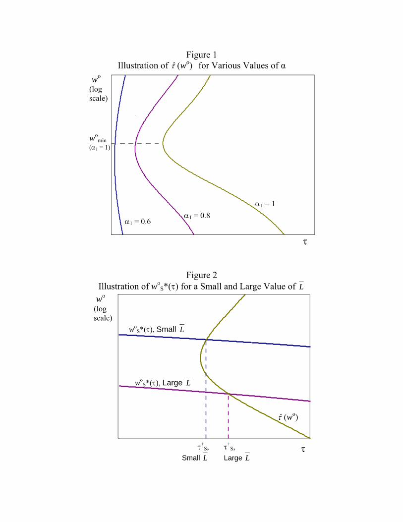
Figure 1 Illustration of (wo) for Various Values of α

Figure 2 Illustration of wo

S*() for a Small and Large Value of L

woS*(), Small L

woS*(), Large L

(wo)

+S,

Large L

+S,

Small L

wo (log scale)

wo (log scale)

1 = 1

1 = 0.8 1 = 0.6

womin

(1 = 1)

Figure 3

Illustration of woVI*() for a Small and Large Value of L

Figure 4

Equilibrium Open-Market Wages in Rent-Seeking Case for Small and Large L

woVI*(), Small L

woVI*(), Large L

+VI,

Large L

+VI,

Small L

(wo)

wo (log scale)

wo*(), Small L

wo*(), Large L

A

B

C

D

(wo)

wo (log scale)

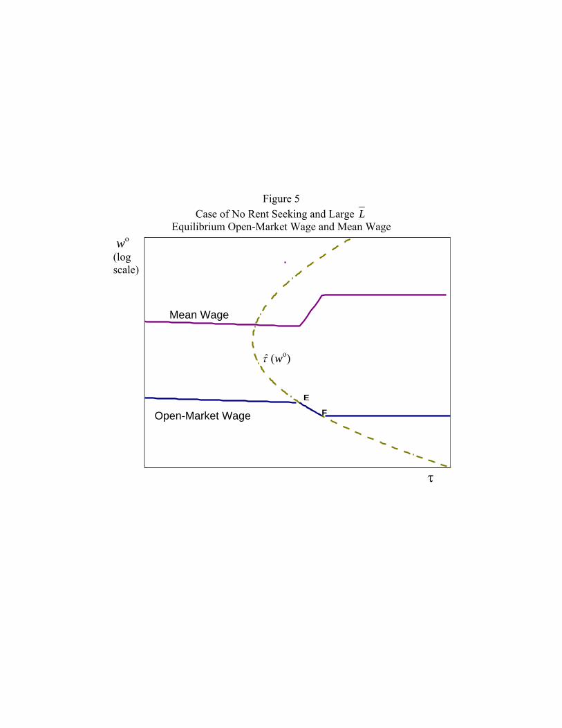
Figure 5

Case of No Rent Seeking and Large L Equilibrium Open-Market Wage and Mean Wage

Open-Market Wage

Mean Wage

E

F

(wo)

wo (log scale)