Embed Size (px)
Citation preview

A Thermodynamically-Consistent Non-Ideal Stochastic Hard-Sphere Fluid
Aleksandar Donev,1, 2 Berni J. Alder,1 and Alejandro L. Garcia3
1Lawrence Livermore National Laboratory,
P.O.Box 808, Livermore, CA 94551-99002Center for Computational Science and Engineering,
Lawrence Berkeley National Laboratory, Berkeley, CA, 947203Department of Physics, San Jose State University, San Jose, California, 95192
A grid-free variant of the Direct Simulation Monte Carlo (DSMC) method is proposed,
named the Isotropic DSMC (I-DSMC) method, that is suitable for simulating dense fluid
flows at molecular scales. The I-DSMC algorithm eliminates all grid artifacts from the tradi-
tional DSMC algorithm; it is Galilean invariant and microscopically isotropic. The stochastic
collision rules in I-DSMC are modified to yield a non-ideal structure factor that gives con-
sistent compressibility, as first proposed in [Phys. Rev. Lett. 101:075902 (2008)]. The
resulting Stochastic Hard Sphere Dynamics (SHSD) fluid is empirically found to have the
same pair correlation function as a deterministic Hamiltonian system of penetrable spheres
interacting with a linear core pair potential, well-described by the hypernetted chain (HNC)
approximation. We apply a stochastic Enskog kinetic theory to the SHSD fluid to obtain
estimates for the transport coefficients that are in excellent agreement with particle sim-
ulations over a wide range of densities and collision rates. The fluctuating hydrodynamic
behavior of the SHSD fluid is verified by comparing its dynamic structure factor against
theory based on the Landau-Lifshitz Navier-Stokes equations. We also study the Brownian
motion of a nano-particle suspended in an SHSD fluid and find a long-time power-law tail
in its velocity autocorrelation function consistent with hydrodynamic theory and molecular
dynamics calculations.
With the increased interest in nano- and micro-fluidics, it has become necessary to develop
tools for hydrodynamic calculations at the atomistic scale [1, 2]. There are several issues present
in microscopic flows that are difficult to account for in models relying on the continuum Navier-
Stokes equations. Firstly, it is complicated to deal with boundaries and interfaces in a way that
consistently accounts for the bidirectional coupling between the flow and (moving) complex surfaces
or suspended particles. Furthermore, it is not trivial to include thermal fluctuations in Navier-
Stokes solvers [3–5], and in fact, most of the time the fluctuations are not included even though
they can be very important at instabilities [6] or in driving the dynamics of suspended objects
[7, 8]. Finally, since the grid cell sizes needed to resolve complex microscopic flows are small, a
2
large computational effort is needed even for continuum solvers. An alternative is to use particle-
based methods, which are explicit and unconditionally stable and rather simple to implement. The
fluid particles are directly coupled to the microgeometry, for example, they directly interact with
the beads of a polymer chain. Fluctuations occur naturally and the algorithm may be designed to
give the correct spatio-temporal correlations.
Several particle methods have been described in the literature. The most accurate but also most
expensive is molecular dynamics (MD) [9], and several coarse-grained models have been developed,
such as dissipative particle dynamics (DPD) [10] and multi-particle collision dynamics (MPCD)
[11, 12], each of which has its own advantages and disadvantages [13]. Our method, first proposed
in Ref. [14], is based on the Direct Simulation Monte Carlo (DSMC) algorithm of Bird [15]. The
key idea behind DSMC is to replace deterministic interactions between the particles with stochastic
momentum exchange (collisions) between nearby particles. While DSMC is usually viewed as a
kinetic Monte Carlo algorithm for solving the Boltzmann equation for a low-density gas, it can also
be viewed as an alternative to the expensive MD in cases where an approximate (coarse-grained)
treatment of the molecular transport is appropriate. The stochastic treatment of collisions makes
the algorithm much simpler and faster than MD, while preserving the essential ingredients of
fluctuating hydrodynamics: local momentum conservation, linear momentum exchange on length
scales comparable to the particle size, and a similar fluctuation spectrum.
Being composed of point particles, the DSMC fluid has no internal structure, has an ideal gas
equation of state (EOS), and is thus very compressible. As a consequence, the density fluctuations
in DSMC are significantly larger than those in realistic liquids. Furthermore, the speed of sound
is small (comparable to the average speed of the particles) and thus subsonic (Mach number less
than one) flows are limited to relatively small Reynolds numbers1. Efforts have been undertaken to
develop coarse-grained models that have greater computational efficiency than brute-force MD and
that have a non-ideal EOS, such as the Lattice-Boltzmann (LB) method [16], DPD [17], MPCD
[18, 19]. The Consistent Boltzmann Algorithm (CBA) [20, 21], as well as algorithms based on the
Enskog equation [22, 23], have demonstrated that DSMC fluids can have dense-fluid compressibility,
however, they did not achieve thermodynamic consistency between the equation of state and the
fluid structure.
1 For a low-density gas the Reynolds number is Re ≈ M/K, where M = vflow/c is the Mach number, and theKnudsen number K = λ/L is the ratio between the mean free path λ and the typical obstacle length L. Thisshows that subsonic flows can only achieve high Re flows for small Knudsen numbers, i.e., large numbers of DSMCparticles.

3
In this paper we describe a generalization of the traditional DSMC algorithm suitable for dense
fluid flows. By a dense fluid we mean a fluid where the mean free path is small compared to the
typical inter-atomic distance. As a first step, inspired by common practice in molecular dynamics,
we introduce a grid-free Isotropic DSMC (I-DSMC) method that eliminates all grid artifacts from
traditional DSMC, notably the lack of Galilean invariance and non-isotropy. The I-DSMC fluid is
still an ideal fluid just like the traditional DSMC fluid, that is, it has an the equation of state of an
ideal gas and does not have an internal structure as do liquids. Secondly, by biasing the collision
kernel in I-DSMC to only allow stochastic collisions between approaching particles, we obtain the
Stochastic Hard-Sphere Dynamics (SHSD) algorithm that is thermodynamically consistent (i.e., the
direct calculation of compressibility from density fluctuations agrees with the density derivative of
pressure). The SHSD algorithm is related to previous algorithms for solving the Enskog kinetic
equation [22, 23], and can be viewed as a more-efficient variable-diameter stochastic modification
of the traditional hard-sphere molecular dynamics [24].
In the SHSD algorithm randomly chosen pairs of approaching particles that lie less than a
given diameter of each other undergo collisions as if they were hard spheres of diameter equal
to their actual separation. The SHSD fluid is shown to be non-ideal, with pair correlations and
equation of state equivalent to that of a deterministic (Hamiltonian) fluid where penetrable spheres
effectively interact with a repulsive linear core pairwise potential. We theoretically demonstrate
this correspondence at low densities. Remarkably, we numerically find that this effective interaction
potential, similar to the quadratic core potential used in many DPD variants, is valid at higher
densities as well, and conjecture that the SHSD fluid has pairwise correlations that are identical to
those of the linear core fluid. If our empirically-supported conjecture is correct, the SHSD fluid, as
DPD, is intrinsically thermodynamically-consistent since it satisfies the virial theorem.
The equivalence of the structure of the SHSD fluid with the linear core fluid enables us to use
the Hypernetted Chain (HNC) approximation, as recommended in Ref. [25], to obtain theoretical
estimates for the pair correlation and static structure factor that are in excellent agreement with
numerical results. These further enable us to use the Enskog-like kinetic theory developed in Ref.
[26] to obtain accurate theoretical estimates of the transport properties of the SHSD fluid that
are also shown to be in excellent agreement with numerics even at relatively high densities. At
lower densities the HNC approximation is not necessary and explicit expressions for the transport
coefficients can be obtained similarly to what has been done using Green-Kubo approach for other
DSMC variants [20] and MPCD [13, 18, 27].
We numerically demonstrate that the hydrodynamics of the SHSD fluid is consistent with the

4
equations of fluctuating hydrodynamics when the appropriate equation of state is taken into ac-
count. Specifically, we compare the measured dynamic structure factors with that obtained from
the linearized fluctuating Navier-Stokes equations. We also calculate the velocity autocorrelation
function (VACF) for a large hard spherical bead suspended in an SHSD fluid, demonstrating the
existence of long-time tails as predicted by hydrodynamics and found in MD simulations. The tail
is found to be in quantitative agreement with theory at lower densities, but a discrepancy is found
at higher densities, possibly due to the strong structuring of the dense SHSD fluid.
We begin by introducing a grid-free variant of the DSMC algorithm in Section I. This Isotropic
DSMC algorithm simulates a stochastic particle system where particles closer than a particle di-
ameter collide with a certain rate. By biasing the collision kernels to favor head-on collisions of
particles, as in the hard-sphere fluid, we obtain a non-ideal stochastic fluid in Section II. We de-
velop an Enskog-like kinetic theory for this Stochastic Hard Sphere Dynamics (SHSD) system in
Section II A, which requires as input the pair correlation function. In Section II B we discover that
the SHSD fluid is thermodynamically consistent with a fluid of penetrable linear core spheres, and
use this equivalence to compute the pair correlation function of the SHSD fluid using the HNC
approximation. In Section III we show several numerical results, including a comparison with the-
ory for the transport coefficients and for the dynamic structure factor, as well as a study of the
hydrodynamic tails in the velocity autocorrelation of a bead suspended in an SHSD fluid.
I. ISOTROPIC DSMC
The traditional DSMC algorithm [15, 28] starts with a time step where particles are propa-
gated advectively, r′i = ri + vi∆t, and sorted into a grid of cells. Then, for each cell c a certain
number Ncoll ∼ ΓscNc(Nc − 1)∆t of stochastic collisions are executed between pairs of particles
randomly chosen from the Nc particles inside the cell, where the collision rate Γsc is chosen based
on kinetic theory. The conservative stochastic collisions exchange momentum and energy between
two particles i and j that is not correlated with the actual positions of the particles. Typically the
probability of collision is made proportional to the magnitude of the relative velocity vr = |vij | by
using a conventional rejection procedure.
Traditional DSMC suffers from several grid artifacts, which become pronounced when the mean
free path becomes comparable to the DSMC cell size. Firstly, the method is not Galilean invariant
unless the grid of cells is shifted randomly before each collision step, as typically done in the MPCD
algorithm [11, 12] for the same reason. This shifting is trivial in a purely particle simulation with

5
periodic boundary conditions, but it causes implementation difficulties when boundaries are present
and also in particle-continuum hybrids [29]. Furthermore, traditional DSMC, unlike MD, is not
microscopically isotropic and does not conserve angular momentum, leading to an anisotropic
collisional stress tensor. Instead of trying to work around these grid artifacts, as done for non-ideal
MPCD in Refs. [18, 19], we have chosen to modify the traditional DSMC algorithm to make the
dynamics grid-free.
To ensure isotropy, all particle pairs within a collision diameter D (i.e., overlapping particles if
we consider the particles to be spheres of diameter D) are considered as potential collision partners
even if they are in neighboring cells. In this way, the grid is only used as a tool to find neighboring
particles efficiently, but does not otherwise affect the properties of the resulting stochastic fluid,
just as is molecular dynamics. Such a grid-free DSMC variant, which we will call the Isotropic
Direct Simulation Monte Carlo (I-DSMC) method, is suitable for hydrodynamics of dense fluids,
where the mean free path is comparable or even smaller than D, unlike the original DSMC which
targets the dilute limit. It is important to point out, however, that the I-DSMC is not meant to be a
replacement for traditional DSMC for rarified gas flows. In particular, the computational efficiency
is reduced by a factor of 2−4 over traditional DSMC due to the need to search neighboring cells for
collision partners in addition to the current cell. This added cost is not justified at low densities,
where the grid artifacts of traditional DSMC are small. Furthermore, the I-DSMC method is
not intended as a solver for the Boltzmann equation, which was the primary purpose of traditional
DSMC [30, 31]. Rather, in the limit of small time steps, the I-DSMC method simulates the following
stochastic particle system: Particles move ballistically in-between collisions. While two particles i
and j are less than a diameter D apart, rij ≤ D, there is a probability rate χD−1Kc(vij , rij) for
them to collide and change velocities without changing their positions, where Kc is some function
of the relative position and velocity of the pair, and the dimensionless cross-section factor χ sets
the collisional frequency. Because the particles are penetrable, D and χ may be interpreted as the
range and strength, respectively, of the interaction potential. After the collision, the pair center-
of-mass velocity does not change, ensuring momentum conservation, while the relative velocity
is drawn from a probability density Pc(v′ij ; vij , rij), such that
∥∥∥v′ij
∥∥∥ = ‖vij‖ so kinetic energy is
conserved.
Once the pre- and post-collision kernels Kc and Pc are specified, the properties of the resulting
I-DSMC fluid are determined by the cross-section factor χ and the density (hard-sphere volume
fraction) φ = πND3/(6V ), where N is the total number of particles in the simulation volume
V . Compare this to the deterministic hard-sphere fluid, whose properties are determined by the

6
volume fraction φ alone. It is convenient to normalize the collision kernel Kc so that for an ideal
gas with a Maxwell-Boltzmann velocity distribution the average collisional rate would be χ times
larger than that of a gas of hard spheres of diameter D at low densities, φ � 1. Two particular
choices for the pre-collision kernel Kc that we use in practice are:
Traditional DSMC collisions (Traditional I-DSMC ideal fluid), for which the probability of colli-
sion is made proportional to the magnitude of the relative velocity vrel = ‖vij‖, Kc = 3vrel/4.
We use this kernel mainly for comparison with traditional DSMC.
Maxwell collisions (Maxwell I-DSMC ideal fluid), for which Kc = 3vrel/4 = 3√kBT0/πm, where
vrel is the average relative velocity at equilibrium temperature T0. Since Kc is a constant, all
pairs collide at the same rate, independent of their relative velocity. This kernel is not realistic
and may lead to unphysical results in cases where there are large density and temperature
gradients, however, it is computationally most efficient since there is no rejection based
on relative velocity. We therefore prefer this kernel for problems where the temperature
dependence of the transport properties is not important, and what we will typically mean
when we say I-DSMC without further qualification.
Other collision kernels may be used in I-DSMC, though we will not consider them here [28].
We typically chose the traditional DSMC post-collisional kernel Pc in which the direction of the
post-collisional relative velocity is randomized so as to mimic the average distribution of collision
impact parameters in a low-density hard-sphere gas. Specifically, in three dimensions the relative
velocity is rotated uniformly independent of rij [15]. If one wishes to microscopically conserve
angular momentum in I-DSMC then the post-collisional kernel has to use the actual positions of
the colliding particles. Specifically, the component of the relative velocity perpendicular to the line
joining the colliding particles should remain unchanged, while the parallel component should be
reversed.
Note that a pairwise Anderson thermostat proposed within the context of MD/DPD by Lowe [32]
adds I-DSMC-like collisions to ordinary MD. In addition to algorithmic differences with I-DSMC,
in Lowe’s method the post-collisional kernel is such that it preserves the normal component of the
relative velocity (thus conserving angular momentum), while the parallel component is thermalized
by drawing from a Maxwell-Boltzmann distribution. We strive to preserve exact conservation of
both momentum and energy in the collision kernels we use, without artificial energy transport via
thermostating.

7
With a finite time step, the I-DSMC method can be viewed as a time-driven kinetic Monte Carlo
algorithm to solve the Master Equation for the stochastic particle system described above. Unlike
the singular kernel in the Boltzmann equation, this Master Equation has a mollified collision kernel
with a finite compact support D [26, 33]. The traditional DSMC method also mollifies the collision
kernel by considering particles within the same collision cell, of size Lc, as possible collision partners.
This DSMC cell size is much larger than a molecular diameter, Dm, in fact, for low densities it is a
fraction (typically a quarter) of the mean free path. The molecular properties enter in traditional
DSMC only in the form of collisional cross-sections σ ∼ D2m. In light of this, for rarified gas flows,
the collision diameter D in I-DSMC should be considered the equivalent of the cell length Lc, and
not Dm. Traditional DSMC is designed to reproduce a collision rate per particle per unit time
equal to the Boltzmann rate, ΓB(Dm) = CD2m, where C is a constant. The I-DSMC method is
designed to reproduce a collision rate
ΓI−DSMC = χΓB(D) = χCD2,
and therefore by choosing
χ = χB =(Dm
D
)2
we get ΓI−DSMC = ΓB(Dm). Therefore, if I-DSMC is used to simulate the transport in a low-
density gas of hard-sphere of diameter Dm, the collision diameter D should be chosen to be some
fraction of the mean free path λ (say, D ≈ λ/4 � Dm), and the cross-section factor set to
χB ∼ (Dm/λ)2 � 1. At higher densities χB starts becoming comparable to unity and thus it is no
longer possible to separate the kinetic and collisional time scales as assumed in traditional DSMC.
Note that I-DSMC is designed for dense fluids so while it is possible to apply it in simulating
rarefied gases it will not be as computationally efficient as traditional DSMC.
A. Performing Stochastic Collisions
In I-DSMC, stochastic collisions are processed at the begining of every time step of duration ∆t,
and then each particle i is streamed advectively with constant velocity vi. During the collision step,
we need to randomly and without bias choose pairs of overlapping particles for collision, given the
current configuration of the system. This can be done, as in traditional DSMC, using a rejection
Monte Carlo technique. Specifically, we need to choose a large number N (tot)tc = Γ(tot)
tc Npairs∆t of
trial collision pairs, and then accept the fraction of them that are actually overlapping as collision

8
candidates. Here Npairs is the number of possibly-overlapping pairs, for example, as a first guess
one can include all pairs, Npairs = N(N−1)/2. The probability for choosing one of the overlapping
pairs as a collision candidate is simply Γ(tot)tc ∆t. If the probability of accepting a candidate pair
ij for an actual collision is p(acc)ij and ∆t is sufficiently small, then the probability rate to actually
collide particles i and j while they are overlapping approaches Γij = p(acc)ij Γ(tot)
tc . The goal is to
choose the trial collision frequency Γ(tot)tc and p
(acc)ij such that Γij = χD−1Kc(vij , rij).
The efficiency of the algorithm is increased if the probability of accepting trial collisions is
increased. In order to increase the acceptance probability, one should reduce Npairs to be closer to
the number of actually overlapping pairs, ideally, one would build a list of all the overlapping pairs
(making Npairs linear instead of quadratic in N). This is however expensive, and a reasonable
compromise is to use collision cells similarly to what is done in classical DSMC and also MD
algorithms. Namely, the spatial domain of the simulation is divided into cells of length Lc ' D,
and for each cell a linked list Lc of all the particles in that cell is maintained. All pairs of particles
that reside in the same or neighboring cells are considered as potential collision partners, and here
we include the cell itself in its list of neighboring cells, i.e., each cell has 3d neighbors, where d is
the spatial dimension.
To avoid any spatial correlations (inhomogeneity and non-isotropy), trial collision pairs should
be chosen at random one by one. This would require first choosing a pair of neighboring cells with
the correct probability, and then choosing a particle from each cell (rejecting self-collisions). This
is rather expensive to do, especially at lower χ, when few actual collisions occur at each time step,
and we have therefore chosen to use a method that introduces a small bias each time step, but is
unbiased over many time steps. Specifically, we visit the cells one by one and for each cell c we
perform N(c)tc = Γ(c)
tc NcNp∆t trial collisions between one of the Nc particles in that cell and one
of the Np particles in the 3d neighboring cells, rejecting self-collisions. Here Γ(c)tc is a local trial
collision rate and it may depend on the particular cell c under consideration. Note that each of
the Nc(Nc − 1) trial pairs ij where both i and j are in cell c is counted twice, and similarly, any
pair where i and j are in different cells c and c′ is included as a trial pair twice, once when each of
the cells c and c′ is considered. Also note that it is important not to visit the cells in a fixed order
during every time step. Unlike in traditional cells, where cells are independent of each other and
can be visited in an arbitrary order (even in parallel), in I-DSMC it is necessary to ensure isotropy
by visiting the cells in a random order, different every time step.
For the Maxwell pre-collision kernel, once a pair of overlapping particles i and j is found
a collision is performed without additional rejection, therefore, we set Γ(c)tc = χD−1Kc/2 =

9
3χ(2D)−1√kBT0/πm = const; note that we have divided by two because of the double count-
ing of each trial pair. For the traditional pre-collision kernel, and, as we shall see shortly, the
SHSD pre-collision kernel, additional rejection based on the relative velocity vij is necessary. As
in the traditional DSMC algorithm, we estimate an upper bound for the maximal value of the
pre-collision kernel K(max)c among the pairs under consideration and set Γ(c)
tc = χD−1K(max)c /2.
We then perform an actual collision for the trial pair ij with probability
pcij = Kc(vij , rij)/K(max)c ,
giving the correct collision probability for every overlapping pair of particles. For the traditional
pre-collision kernel K(max)c = 3v(max)
rel /4, where v(max)rel is as tight an estimate of the maximum
relative speed as possible. In the traditional DSMC algorithm v(max)rel is a global bound obtained
by simply keeping track of the maximum particle speed vmax and taking v(max)rel = 2vmax [15]. In
I-DSMC, we obtain a local estimate of v(max)rel for each cell c that is visited, thus increasing the
acceptance rate and improving efficiency.
Algorithm 1 specifies the procedure for performing collisions in the I-DSMC method. The
algorithm is to a large degree collision-kernel independent, and in particular, the same algorithm
is used for ideal and non-ideal stochastic fluids. As already explained, the size of the cells should
be chosen to be as close as possible but still larger than the particle diameter D. The time step
should be chosen such that a typical particle travels a distance l∆t ≈ vth∆t ∼ Dδt, where the
typical thermal velocity vth =√kBT0/m and δt is a dimensionless time step, which should be
kept reasonably smaller than one, for example, δt / 0.25. It is also important to ensure that each
particle does not, on average, undergo more than one collision per time step; we usually keep the
number of collisions per particle per time step less than one half. Since a typical value of the
pre-collision kernel is Kc ∼ vth, the number of collisions per particle per time-step can easily be
seen to be on the order of
Ncps ∼ χvthD· NVVp ·∆t = χφδt,
where Vp ∼ D3 is a particle volume. Therefore, unless χφ� 1, choosing a small dimensionless time
step δt will ensure that the collisional frequency is not too large, Ncps � 1. With these conditions
observed, we find little dependence of the fluid properties on the actual value of δt.
Algorithm 1: Processing of stochastic collisions between overlapping particles at a time-step in
the I-DSMC method.

10
1. Sample a random permutation of the cell numbering P.
2. Visit the cells one by one in the random order given by P. For each cell c, do the following steps if
the number of particles in that cell Nc > 0, otherwise move on to the next cell.
3. Build a list L1 of the Nc particles in the cell and at the same time find the largest particle speed in
that cell vmax1 . Also keep track of the second largest speed in that cell vmax2 , which is an estimate of
the largest possible speed of a collision partner for the particle with speed vmax1 .
4. Build a list of the Np particles in the set of 3d cells that neighbor c, including the cell c itself and
respecting the proper boundary conditions. Also update vmax2 if any of the potential collision partners
not in cell c have speeds greater than vmax2 .
5. Determine the number of trial collisions between a particle in cell c and a neighboring particle by
rounding to an integer [15] the expected value
Ntc = ΓtcNcNp∆t,
where ∆t is the time step. Here the local trial collision rate is
Γtc =χKmax
c
2D,
where Kmaxc is an upper bound for the pre-collision kernel among all candidate pairs. For Maxwell
collisions Kmaxc = 3
√kBT0/πm, and for traditional collisions Kmax
c = 3v(max)rel /4, where v(rel)
max =
(vmax1 + vmax2 ) is a local upper bound on the relative speed of a colliding pair.
6. Perform trial collisions by randomly selecting Ntc pairs of particles i ∈ L1 and j ∈ L2. For each pair,
do the following steps if i 6= j:
(a) Calculate the distance lij between the centroids of particles i and j, and go to the next pair if
lij > D.
(b) Calculate the collision kernel Kcij = Kc(vij , rij), and go to the next pair if Kc
ij = 0.
(c) Sample a random uniform variate 0 < r ≤ 1 and go to the next pair if Kcij ≤ rKmax
c (note that
this step can be skipped in Maxwell I-DSMC since Kcij = Kmax
c ).
(d) Process a stochastic collision between the two particles by updating the particle velocities
by sampling the post-collision kernel Pc(v′
ij ; vij , rij). For ideal fluids we perform the usual
stochastic DSMC collision by randomly rotating vij to obtain v′
ij , independent of rij .

11
II. STOCHASTIC HARD SPHERE DYNAMICS
The traditional DSMC fluid has no internal structure so it has an ideal gas equation of state
(EOS), p = PV/NkBT = 1, and is thus very compressible. As for the classical hard-sphere fluid,
the pressure of fluids with stochastic collisions consists of two parts, the usual kinetic contribution
that gives the ideal-gas pressure pk = 1, and a collisional contribution proportional to the virial
pc ∼⟨(vij · rij)′ − (vij · rij)
⟩c, where the average is over stochastic collisions and primes denote
post-collisional values. The virial vanishes for collision kernels where velocity updates and positions
are uncorrelated, as in traditional DSMC, leaving only the ideal-gas kinetic contribution. In order
to introduce a non-trivial equation of state it is necessary to either give an additional displacement
∆rij to the particles that is parallel to vij , or to bias the momentum exchange ∆pij = m∆vij to be
(statistically) aligned to rij . The former approach has already been investigated in the Consistent
Boltzmann Algorithm (CBA) [20, 21]. This algorithm was named “consistent” because both the
transport coefficients and the equation of state are consistent with those of a hard-sphere fluid to
lowest order in density, unlike traditional DSMC which only matches the transport coefficients.
However, CBA is not thermodynamically consistent since it modifies the compressibility without
affecting the density fluctuations (i.e., the structure of the fluid is still that of a perfect gas).
Here we explore the option of biasing the stochastic momentum exchange based on the position
of the colliding particles. What we are trying to emulate through this bias is an effective repulsion
between overlapping particles. This repulsion will be maximized if we make ∆pij parallel to rij ,
that is, if we use the hard-sphere collision rule Pc(v′ij ; vij , rij) = δ(vij+2vnrij), where vn = −vij ·rij
is the normal component of the relative velocity. Explicitly, we collide particles as if they are elastic
hard spheres of diameter equal to the distance between them at the time of the collision,
v′i =vi + vnrij
v′j =vj − vnrij . (1)
Such collisions produce a positive virial only if the particles are approaching each other, i.e., if
vn > 0, therefore, we reject collisions among particles that are moving apart, Kc(vij , rij) ∼ Θ(vn),
where Θ denotes the Heaviside function. Note that the hard-sphere post-collision rule (1) strictly
conserves angular momentum in addition to linear momentum and energy and can be used with
other pre-collision kernels (e.g., Maxwell) if one wishes to conserve angular momentum.
To avoid rejection of candidate collision pairs and thus make the algorithm most efficient, it
would be best if the pre-collision kernel Kc is independent of the relative velocity as for Maxwell

12
collisions. However, without rejection based on the normal vn or relative vr speeds, fluctuations of
the local temperature Tc would not be consistently coupled to the local pressure. Namely, without
rejection the local collisional frequency Γsc would be independent of Tc and thus the collisional
contribution to the pressure pc ∼ 〈∆vij · rij〉c ∼ Γsc√Tc would be pc ∼
√Tc instead of pc ∼ Tc,
as is required for a fluid with no internal energy [18, 19]. Instead, as for hard spheres, we require
that Γsc ∼√Tc, which is satisfied if the collision kernel is linear in the magnitude of the relative
velocity. For DSMC the collisional rules can be manipulated arbitrarily to obtain the desired
transport coefficients, however, for non-ideal fluids thermodynamic requirements eliminate some
of the freedom. This important observation has not been taken into account in other algorithms
that randomize hard-sphere molecular dynamics [34], but has been used in the non-ideal MPCD
algorithm in order to obtain thermodynamic consistency [18, 19].
There are two obvious choices for a pre-collision kernel that are linear in the magnitude of the
relative velocity. One is to use the relative speed, Kc ∼ vr, as in the traditional DSMC algorithm,
and the other is to use the hard-sphere pre-collision kernel, Kc ∼ vn. We have chosen to make the
collision probability linear in the normal speed vn, specifically, we take Kc = 3vnΘ(vn) to define the
Stochastic Hard-Sphere Dynamics (SHSD) fluid, similarly to what has previously been done in the
Enskog DSMC algorithm [22, 23] and in non-ideal MPCD [18, 19]. These choices for the collision
kernels make the SHSD fluid identical to the one proposed in Ref. [33] for the purposes of proving
convergence of a microscopic model to the Navier-Stokes equations. Specifically, the singular
Boltzmann hard-sphere collision kernel is mollified in Ref. [33] to obtain the SHSD collision kernel
and then the low-density hydrodynamic limit is considered.
The non-ideal SHSD fluid is simulated by the I-DSMC method, in the limit of sufficiently small
time steps. However, it is important to observe that the SHSD fluid is defined independently of
any temporal discretization used in computer simulations, just like a Hamiltonian fluid is defined
through the equations of motion independently of Molecular Dynamics (MD). To summarize, in
the SHSD algorithm we use the following collision kernels in Algorithm 1:
Kc =3vnΘ(vn) and K(max)c = 3v(rel)
max
Pc(v′ij) =δ(vij + 2vnrij)
where vn = −vij · rij .
Note that considering particles in neighboring cells as collision partners is essential in SHSD in
order to ensure isotropy of the collisional (non-ideal) component of the pressure tensor. It is also
important to traverse the cells in random order when processing collisions, as well as to ensure
13
a sufficiently small time step is used to faithfully simulate the SHSD fluid. Note that the SHSD
algorithm strictly conserves both momentum and energy independent of the time step.
A. Enskog Kinetic Theory
In this section we develop some kinetic equations for the SHSD fluid that are inspired by the
Enskog theory of hard-sphere fluids. Remarkably, it turns out that these sorts of kinetic equations
have already been studied in the literature for purely theoretical purposes.
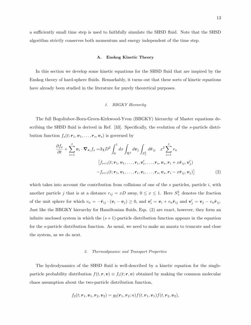
1. BBGKY Hierarchy
The full Bogoliubov-Born-Green-Kirkwood-Yvon (BBGKY) hierarchy of Master equations de-
scribing the SHSD fluid is derived in Ref. [33]. Specifically, the evolution of the s-particle distri-
bution function fs(t; r1,v1, . . . , rs,vs) is governed by
∂fs∂t
+s∑i=1
vi ·∇rifs =3χD2
∫ 1
0dx
∫R3
dvj
∫S2
+
drij x2s∑i=1
vn
[fs+1(t; r1,v1, . . . , ri,v
′i, . . . , rs,vs, ri + xrij ,v
′j)
−fs+1(t; r1,v1, . . . , ri,vi, . . . , rs,vs, ri − xrij ,vj)]
(2)
which takes into account the contribution from collisions of one of the s particles, particle i, with
another particle j that is at a distance rij = xD away, 0 ≤ x ≤ 1. Here S2+ denotes the fraction
of the unit sphere for which vn = −rij · (vi − vj) ≥ 0, and v′i = vi + vnrij and v′j = vj − vnrij .
Just like the BBGKY hierarchy for Hamiltonian fluids, Eqs. (2) are exact, however, they form an
infinite unclosed system in which the (s+ 1)-particle distribution function appears in the equation
for the s-particle distribution function. As usual, we need to make an anzatz to truncate and close
the system, as we do next.
2. Thermodynamic and Transport Properties
The hydrodynamics of the SHSD fluid is well-described by a kinetic equation for the single-
particle probability distribution f(t, r,v) ≡ f1(t; r,v) obtained by making the common molecular
chaos assumption about the two-particle distribution function,
f2(t; r1,v1, r2,v2) = g2(r1, r2;n)f(t, r1,v1)f(t, r2,v2),

14
where g2(ri, rj ;n) is the non-equilibrium pair distribution function that is a functional of the local
number density n(r). At global equilibrium n(r) = const and g2 ≡ g2(rij) depends only on the
radial distance once the equilibrium density n and cross-section factor χ are specified. Substituting
the above assumption for f2 in the first equation of the BBGKY hierarchy (2), we get a stochastic
revised Enskog equation of the form studied in Ref. [26],
∂f(t, r,v)∂t
+ v ·∇rf(t, r,v) =3χD2
∫ 1
0dx
∫R3
dw
∫S2
+
de x2vn
[g2(r, r + xe;n)f(t, r,v′)f(t, r + xe,w′)
−g2(r, r − xe;n)f(t, r,v)f(t, r − xe,w)]
(3)
where vn = −e · (v −w) ≥ 0, v′ = v + evn and w′ = w − evn.
The standard second-order Chapman-Enskog expansion has been carried out for the “stochastic
Enskog” equation of the same form as Eq. (3) in Ref. [26], giving the equation of state (EOS)
p = PV/NkBT , and estimates of the diffusion coefficient ζ, the shear η and bulk ηB viscosities,
and thermal conductivity κ of the SHSD fluid. The expressions in Ref. [26] ultimately express
the transport coefficients in terms of various dimensionless integer moments of the pair correlation
function g2(x = r/D), xk =∫ 1
0 xkg2(x)dx, specifically,
p− 1 =12φχx3, (4)
ζ/ζ0 =√π
48φχx2, (5)
ηB/η0 =48φ2χx4
π3/2, (6)
η/η0 =5
48√πχx2
(1 +24φχx3
5)2 +
35ηB, and (7)
κ/κ0 =25
64√πχx2
(1 +36φχx3
5)2 +
32ηB, (8)
where ζ0 = D√kBT/m, η0 = D−2
√mkBT and κ0 = kBD
−2√kBT/m are natural units. These
equations are very similar to the ones in the Enskog theory of the hard-sphere fluid except that
various coefficients are replaced with moments of g2(x). In order to use these equations, however,
we need to have a good approximation to the pair correlation function, i.e., to the structure of the
SHSD fluid. It is important to point out that Eq. (4) is exact as it can be derived directly from
the definition of the collisional contribution to the pressure.

15
B. Pair Correlation Function
In this section we study the structure of the SHSD fluid, theoretically at low densities, and then
numerically at higher densities. We find, surprisingly, that there is a thermodynamic correspon-
dence between the stochastic SHSD fluid and a deterministic penetrable-sphere fluid.
1. Low Densities
In order to understand properties of the SHSD fluid as a function of the density φ and the cross-
section factor χ, we first consider the equilibrium pair correlation function g2(r) at low densities,
where correlations higher than pairwise can be ignored. We consider the cloud of point walkers
ij representing the N(N − 1)/2 pairs of particles, each at position r = ri − rj and with velocity
v = vi − vj . If one of these walkers is closer than D to the origin, r ≤ D, and is approaching
the origin, vn > 0, it reverses its radial speed as a stochastic process with a time-dependent rate
Γ = |vn|Γ0, where Γ0 = 3χ/D is the collision frequency. A given walker corresponding to pair ij
also undergoes stochastic spatially-unbiased velocity changes with some rate due to the collisions
of i with other particles. At low densities we can assume that these additional collisions merely
thermalize the velocities to a Maxwell-Boltzmann distribution but not otherwise couple with the
radial dependence of the one-particle distribution function fpairs(v, r) of the N(N − 1)/2 walkers.
Inside the core r ≤ D this distribution of pair walkers satisfies a kinetic equation
∂fpairs∂t
− vn∂fpairs∂r
=
−Γfpairs if vn ≥ 0
Γfpairs if vn < 0= −Γ0vnfpairs, (9)
where the term −Γfpairs is a loss term for approaching pairs due to their collisions, while Γfpairs
is a gain term for pairs that are moving part due to collisions of approaching pairs that then
reverse their radial speed. At equilibrium, ∂fpairs/∂t = 0 and vn cancels on both sides, con-
sistent with choosing collision probability linear in |vn|, giving ∂fpairs/∂r = 3χD−1fpairs. At
equilibrium, the distribution of the point walkers in phase space ought to be of the separable form
fpairs(v, r) = fpairs(vn, r) ∼ g2(r) exp(−mv2n/4kT ), giving dg2(r)/dr = 3χD−1g2(r) for r ≤ D and
zero otherwise, with solution
g2(x = r/D) =
exp [3χ(x− 1)] for x ≤ 1
1 for x > 1(10)
Indeed, numerical experiments confirmed that at sufficiently low densities the equilibrium g2 for
the SHSD fluid has the exponential form (10) inside the collision core. From statistical mechanics

16
we know that for a deterministic Hamiltonian particle system with a pairwise potential U(r) at low
density gU2 = exp[−U(r)/kT ]. Therefore, the low density result (10) is consistent with an effective
linear core pair potential
Ueff (r)/kT = 3χ(1− x)Θ(1− x). (11)
Note that this repulsive potential is similar to the quadratic core potential used in DPD and strictly
vanishes outside of the overlap region, as expected. Also note that the cross-section factor χ plays
the role that U(0)/kT plays in the system of penetrable spheres interacting with a linear core
pairwise potential.
As pointed out earlier, Eq. (4) is exact. At the same time, it is equivalent to the virial theorem
for the linear core potential. Therefore, if the pair correlation functions of the SHSD fluid and the
linear core fluid are truly identical, the pressure of the SHSD fluid is identically equal to that of the
corresponding penetrable sphere system. As a consequence, thermodynamic consistency between
the structure [g2(x) and S(k)] and equation-of-state [p(φ)] is guaranteed to be exact for the SHSD
fluid.
2. Equivalence to the Linear Core Penetrable Sphere System
Remarkably, we find numerically that the effective potential (11) can predict exactly g2(x) at all
densities. In fact, we have numerically observed that the SHSD fluid behaves thermodynamically
identically to a system of penetrable spheres interacting with a linear core pairwise potential for
all φ and χ that we have tried, including densities at which freezing is observed. Figure 1 shows a
comparison between the pair correlation function of the SHSD fluid on one hand, and a Monte Carlo
calculation using the linear core pair potential on the other, at several densities. Also shown is a
numerical solution to the hypernetted chain (HNC) integral equations for the linear core system,
inspired by its success for the Gaussian core model [25]. The excellent agreement at all densities
permits the use of the HNC result in practical applications, notably the calculation of the transport
coefficients via the Enskog-like kinetic theory presented in Section II A 2. We also show the static
structure factor S(k) in Fig. 1, and find very good agreement between numerical results and the
HNC theory, as expected since S(k) can be expressed as the Fourier transform of h(r) = g2(r)− 1.
We have not examined correlations of order higher than pairwise in detail, since the pressure and
transport coefficient estimates that we use depend only on the pair correlation function.
For collision frequencies χ . 1 the structure of the SHSD fluid is quite different from that of

17
0.25 0.5 0.75 1 1.25 1.5 1.75 2
x=r/D
0.25
0.5
0.75
1
g 2(x)
Low density limitHNC linear coreMC linear coreSHSD φ=0.1SHSD φ=0.5SHSD φ=1.0SHSD φ=2.0
0 0.25 0.5 0.75 1 1.25 1.5 1.75 2 2.25 2.5
kD / 2π0
0.25
0.5
0.75
1
1.25
1.5
S(k)
Low density appr. (φ=0.1)HNC linear coreSHSD φ=0.1SHSD φ=0.5SHSD φ=1.0SHSD φ=2.0
Figure 1: (Left) Equilibrium pair correlation function of the SHSD fluid (solid symbols, N = 104 particles
in a cubic periodic box), compared to Monte Carlo simulations (open symbols, N = 104 particles in a cubic
periodic box) and numerical solution of the HNC equations (solid lines) for the linear core system, at various
densities and χ = 1. The low-density approximation corresponding to Eq. (10) is also shown. (Right) The
corresponding static structure factors from SHSD simulations (solid symbols, average of ten snapshots of a
system with N = 105 particles in a cubic periodic box) and HNC calculations (solid lines). The time step
was kept sufficiently small in the SHSD simulations to ensure that the results faithfully represent the SHSD
fluid with time-step errors smaller than the statistical uncertainties, which are on the order of the largest
symbol size except at the smallest x where there is less sampling.
the hard-sphere fluid because the particles inter-penetrate and overlap significantly. Interestingly,
in the limit of infinite collision frequency χ→∞ the SHSD fluid reduces to the hard-sphere (HS)
fluid for sufficiently low densities. In fact, if the density φ is smaller than the freezing point for the
HS system, the structure of the SHSD fluid approaches, as χ increases, that of the HS fluid. For
higher densities, if χ is sufficiently high, crystallization is observed in SHSD, either to the usual
hard-sphere crystals if φ is lower than the close-packing density, or if not, to an unusual partially
ordered state with multiple occupancy per site, typical of weakly repulsive potentials [35]. Monte
Carlo simulations of the linear core penetrable sphere system show identical freezing behavior
with SHSD, confirming the surprising equivalence even at non-fluid densities. This points to a
conjecture that the (unique) stationary solution to the BBGKY hierarchy (2) is the equilibrium
Gibbs distribution,
fEs =∏si=1M(vi)ZN
∫rs+1
. . .
∫rN
exp
−β∑i<j
Ueff (rij)
drs+1 . . . drN ,
where M is a Maxwellian. Further numerical tests of this conjecture could be obtained by per-
forming a detailed comparison of higher-order correlation functions and phase diagrams of the two

18
fluids. However, the unexpected relation between the pair correlation functions of the two fluids,
demonstrated above, is sufficient to enable us to apply well-established liquid state and kinetic
theories to the SHSD fluid.
III. RESULTS
In this Section we perform several numerical experiments with the SHSD algorithm. Firstly, we
compare the theoretical predictions for the transport properties of the SHSD fluid based on the HNC
theory for the linear core penetrable sphere system with results from particle simulations. We then
compute dynamic structure factors and compare them to predictions of fluctuating hydrodynamics.
Finally, we study the motion of a Brownian bead suspended in an SHSD fluid.
A. Thermodynamic and Transport Properties
The equation of state of the SHSD fluid for a given χ is P = p(φ)NkBT/V , where p(φ) is given
in Eq. (4). According to statistical mechanics, the structure factor at the origin is equal to the
isothermal compressibility, that is,
S0 = S(ω = 0, k = 0) = c−2T = (p+ φdp/dφ)−1
where cT = cT√kBT/m is the isothermal speed of sound. In the inset in the top part of Fig. 2, we
directly demonstrate the thermodynamic consistency of SHSD by comparing the compressibility
calculated through numerical differentiation of the pressure, to the structure factor at the origin.
The pressure is easily measured in the particle simulations by keeping track of the total collisional
momentum exchange during a long period, and its derivative was obtained by numerical differen-
tiation. The structure factor is obtained through a temporal average of a Fast Fourier Transform
approximation to the discrete Fourier Transform of the particle positions ‖∑
i exp(−ik · ri)‖2. The
value S(k = 0) is estimated by fitting a parabolic dependence for small k and extrapolating to
k = 0.
As pointed out earlier, the dimensionless time step δt = D/√kBT0/m in the SHSD algorithm
should be kept reasonably small, δt � min[1, (φχ)−1
], in order to faithfully simulate the SHSD
fluid. As the time step becomes too large we expect to see deviations from the correspondence with
the linear core system and thus a violation of thermodynamic consistency. This is indeed observed
in our numerical results, shown in Fig. 2, where we compare the structure factor at the origin as
estimated through the equation of state with that obtained from a direct Fourier transform of the

19
0.25 0.5 0.75 1 1.25 1.5 1.75 2 2.25 2.5
φ1.75
2
2.25
2.5
2.75
(p-1
)/(χ
φ)Low-density limitχ=1.00χ=0.75χ=0.50χ=0.25
0.5 1 1.5 2φ0
0.1
0.2
0.3
0.4
0.5
0.6S(
k=0)
0.25 0.5 0.75 1 1.25 1.5 1.75 2
φ
0.1
0.2
0.3
0.4
0.5
0.6
S(k=
0)
δt=0.025 fluct.δt=0.1 fluct.δt=0.25 fluct.δt=0.5 fluct.δt=0.025 compress.δt=0.1 compress.δt=0.25 compress.δt=0.5 compress.
Figure 2: (Left) Normalized equation of state (p − 1)/(χφ) for the SHSD fluid at several cross-section
factors χ (different symbols, N = 105 particles in a cubic box) compared to theoretical predictions based
on the virial theorem (4) with the HNC approximation to g2(x) (solid lines). The inset compares the
compressibility (p + φdp/dφ)−1 (dashed lines) to the structure factor at the origin S(k → 0) (symbols),
measured using a direct Fourier transform of the particle positions for small k and extrapolating to k = 0.
The dimensionless time step δt = 0.025 is kept constant and small as the density is changed. (Right)
Thermodynamic consistency between the compressibility (lines) and the large-scale density fluctuations
S(k → 0) (symbols) for different dimensionless time steps δt, keeping χ = 1 fixed.
particle positions. We should point out that when discussing thermodynamic consistency one has
to define what is meant by the the derivative dp/dφ. We choose to keep the collisional frequency
prefactor χ and the dimensionless time step δt constant as we change the density, that is, we study
the thermodynamic consistency of a time-discrete SHSD fluid defined by the parameters φ, χ and
δt. The results in Fig. 2 show that there are significant deviations from thermodynamic consistency
when the average number of collisions per particle per time step is larger than one. This happens
at the highest densities for δt & 0.1, but is not a problem at the lowest densities. Nevertheless,
a visible inconsistency is observed even at the lower densities for δt & 0.25, which comes because
particles travel too far compared to their own size during a time step.
Having established that the HNC closure provides an excellent approximation g(HNC)2 ≈ g2
for the pair correlation function of the SHSD fluid, we can obtain estimates for the transport
coefficients by calculating the first four moments of g(HNC)2 (x) and substituting them in the results
of the Enskog kinetic theory presented in Section II A 2. In Figure 3 we compare the theoretical
predictions for the diffusion coefficient ζ and the viscosity η to the ones directly calculated from
SHSD particle simulations. We measure ζ directly from the average mean square displacement
of the particles. We estimate η by calculating the mean flow rate in Poiseuille parabolic flow

20
0.5 0.75 1 1.25 1.5 1.75 2
φ0
1
2
3
4
5
6
7η/
η 0χ=0.25χ=0.50χ=0.75χ=1.00
0 0.1 0.2 0.3 0.4 0.50
0.5
1
Low density limit
0 0.5 1 1.5 2 2.5φ
0.1
0.125
0.15
0.175
0.2
ζ (χ
φ) /
ζ 0
Chapman-EnskogLow density theoryχ=0.25 SHSDχ=0.50χ=0.75χ=1.00
Figure 3: Comparison between numerical results for SHSD at several collision frequencies (different symbols)
with predictions based on the stochastic Enskog equation using the HNC approximation for g2(x) (solid
lines). The low-density approximations are also indicated (dashed lines). (Left) The normalized shear
viscosity η/η0 at high and low densities (inset), as measured using an externally-forced Poiseuille flow.
There are significant corrections (Knudsen regime) for large mean free paths (i.e., at low densities and low
collision rates). (Right) The normalized diffusion coefficient ζ(χφ)/ζ0, as measured from the mean square
displacement of the particles. The time step was kept sufficiently small in the SHSD simulations to ensure
that the results are faithfully represent the SHSD fluid with time-step errors smaller than the statistical and
measurement errors.
between two thermal hard walls due to an applied constant force on the particles2. Surprisingly,
good agreement is found for the shear viscosity at all densities. Similar matching was observed for
the thermal conductivity κ. The corresponding results for the diffusion coefficient show significant
(∼ 25%) deviations for the self-diffusion coefficient at higher densities because of larger corrections
due to higher-order correlations.
B. Dynamic Structure Factors
The hydrodynamics of the spontaneous thermal fluctuations in the SHSD fluid is expected
to be described by the Landau-Lifshitz Navier-Stokes (LLNS) equations for the fluctuating field
U = (ρ0 + δρ, δv, T0 + δT ) linearized around a reference equilibrium state U0 = (ρ0,v0 = 0, T0)
2 Similar results are obtained by calculating the viscous contributions to the kinetic and collisional stress tensorin non-equilibrium simulations of Couette shear flow. This kind of calculation additionally gives the split in theviscosity between kinetic and collisional contributions.

21
[36, 37]. For the SHSD fluid the linearized equation of state is
P = p(φ)NkBT
V≈ (p0 + c2
T
δρ
ρ0+ p0
δT
T0)ρ0c
20,
and there is no internal energy contribution to the energy density,
e ≈ 32NkBT
V= e0 + cvT0δρ+ ρ0cvδT,
where p0 = p(φ0), c0 = kBT/m, and cv = 3kB/2m, giving an adiabatic speed of sound cs = csc0,
where c2s = c2
T + 2p2/3. Omitting the δ’s for notational simplicity, for one-dimensional flows the
LLNS equations take the form
∂tρ
∂tv
∂tT
= − ∂
∂x
ρ0v
c2Tρ−10 ρ+ p0c
20T−10 T
p0c20c−1v v
+∂
∂x
0
ρ−10 η0vx
ρ−10 c−1
v κ0Tx
+∂
∂x
0
ρ−10
√2η0kBT0W
(v)
ρ−10 c−1
v T0
√2κ0kBW
(T )
,(12)
where W (v) and W (T ) are independent spatio-temporal white noise Gaussian fields.
By solving these equations in the Fourier wavevector-frequency domain for U(k, ω) and per-
forming an ensemble average over the fluctuating stresses we can obtain the equilibrium (sta-
tionary) spatio-temporal correlations (covariance) of the fluctuating fields. We express these cor-
relations in terms of the 3 × 3 symmetric positive-definite hydrodynamic structure factor matrix
SH(k, ω) =⟨UU
?⟩
[5]. The hydrostatic structure factor matrix SH(k) is obtained by integrating
SH(k, ω) over all frequencies,
SH(k) =
ρ0c−2T kBT0 0 0
0 ρ−10 kBT0 0
0 0 ρ−10 c−1
v kBT20
. (13)
We use SH(k) for an ideal gas (i.e., for p0 = 1, cT = 1) to non-dimensionalize SH(k, ω), for
example, we express the spatio-temporal cross-correlation between density and velocity through
the dimensionless hydrodynamic structure factor
Sρ,v(k, ω) =(ρ0c−20 kBT0
)− 12(ρ−1
0 kBT0
)− 12 〈ρ(k, ω)v?(k, ω)〉 .
For the non-ideal SHSD fluid the density fluctuations have a spectrum
Sρ(k) =(ρ0c−20 kBT0
)−1 〈ρ(k)ρ?(k)〉 = c−2T ,

22
which only captures the small k behavior of the full (particle) structure factor S(k) (see Fig. 1), as
expected of a continuum theory that does not account for the structure of the fluid. Typically only
the density-density dynamic structure factor is considered because it is accessible experimentally
via light scattering measurements and thus most familiar. However, in order to fully access the
validity of the full LLNS system one should examine the dynamic correlations among all pairs of
variables. The off-diagonal elements of the static structure factor matrix SH(k) vanish because the
primitive hydrodynamic variables are instantaneously uncorrelated, however, they have non-trivial
dynamic correlations visible in the off-diagonal elements of the dynamic structure factor matrix
SH(k, ω).
-7.5 -5 -2.5 0 2.5 5 7.5ω
0
1
2
3
4
5
6
7
8
c T2 S
ρ(k,ω
)
IDSMC φ=0.5, χ=0.62SHSD φ=0.5, χ=1SHSD φ=1, χ=1
Figure 4: Normalized density fluctuations c2TSρ(k, ω) for kD ≈ 0.070 for an ideal Maxwell I-DSMC (φ = 0.5,
χ = 0.62) and two non-ideal SHSD (φ = 0.5, χ = 1 and φ = 1, χ = 1) fluids of similar kinematic viscosity,
as obtained from particle simulations (symbols with parameters , kBT0 = 1, m = 1). The predictions of
the LLNS equations are also shown for comparison in the same color (solid lines). For the SHSD fluid we
obtained the transport coefficients from the Enskog theory with the HNC approximation to g2, while for the
Maxwell I-DSMC fluid we numerically estimated the viscosity and thermal conductivity.
In Figs. 4 and 5 we compare theoretical and numerical results the hydrodynamic structure
factors for the SHSD fluid with χ = 1 at two densities for a small and a medium k value [kD/(2π) ≈
0.01 and 0.08]. In this figure we show selected elements of SH(k, ω) as predicted by the analytical
solution to Eqs. (12) with parameters obtained by using the HNC approximation to g2 in the
Enskog kinetic theory presented in Section II A 2. Therefore, for SHSD the theoretical calculations

23
-100 -75 -50 -25 0 25 50 75 100ω
0
0.05
0.1
0.15
0.2
0.25
0.3
S(k,
ω)
ρ − ρvx - vxvy - vy
T - T
-100 -75 -50 -25 0 25 50 75 100ω
-0.05
-0.025
0
0.025
0.05
S(k,
ω)
ρ − vx
ρ − Tvx - T
Figure 5: Selected diagonal (left panel) and off-diagonal elements (right panel) of the non-dimensionalized
hydrodynamic structure factor matrix SH(k, ω) for a large wavenumber kD ≈ 0.50 for an SHSD fluid at
φ = 1, χ = 1 (symbols), compared to the predictions from the LLNS equations (lines of same color). The
remaining parameters are as in Fig. 4.
of SH(k, ω) do not use any numerical inputs from the particle runs. We also show hydrodynamic
structure factors obtained from particle simulations in a quasi-one-dimensional setup in which the
simulation cell was periodic and long along the x axis, and divided into 60 hydrodynamic cells of
length 5D. Finite-volume averages of the hydrodynamic conserved variables were then calculated
for each cell every 10 time steps and a Fast Fourier Transform used to obtain hydrodynamic
structure factors for several wavenumbers. Figure 4 shows very good agreement between theory
and numerics, and clearly shows the shifting of the two symmetric Brillouin peaks at ω ≈ csk
toward higher frequencies as the compressibility of the SHSD fluid is reduced and the speed of
sound increased. Figure 5 shows that the positions and widths of the side Brillouin peaks and the
width of the central Rayleigh are well-predicted for all elements of SH(k, ω) for a wide range of k
values, demonstrating that the SHSD fluid shows the expected fluctuating hydrodynamic behavior.
C. Brownian Walker VACF
As an illustration of the correct hydrodynamic behavior of the SHSD fluid and the significance
of compressibility, we study the velocity autocorrelation function (VACF) C(t) = 〈vx(0)vx(t)〉 for
a single neutrally-buoyant hard sphere Brownian bead of mass M and radius R suspended in an
SHSD fluid of mass density ρ. This problem is relevant to the modeling of polymer chains or
(nano)colloids in solution, and led to the discovery of a long power-law tail in C(t) [38] which has
since become a standard test for hydrodynamic behavior of solvents [27, 39, 40]. Here the fluid
particles interact via stochastic collisions, exactly as in I-DSMC. The interaction between fluid

24
particles and the bead is treated as if the SHSD particles are hard spheres of diameter Ds, chosen
to be somewhat smaller than their interaction diameter with other fluid particles (specifically, we
use Ds = D/4) for computational efficiency reasons, using an event-driven algorithm [41]. Upon
collision with the bead the relative velocity of the fluid particle is reversed in order to provide a
no-slip condition at the surface of the suspended sphere [40, 41] (slip boundaries give qualitatively
identical results). For comparison, an ideal I-DSMC fluid of comparable viscosity is also simulated.
Theoretically, C(t) has been calculated from the linearized (compressible) fluctuating Navier-
Stokes (NS) equations [40]. The results are analytically complex even in the Laplace domain, how-
ever, at short times an inviscid compressible approximation applies. At large times the compress-
ibility does not play a role and the incompressible NS equations can be used to predict the long-time
tail. At short times, t < tc = 2R/cs, the major effect of compressibility is that sound waves gener-
ated by the motion of the suspended particle carry away a fraction of the momentum, so that the
VACF quickly decays from its initial value C(0) = kBT/M to C(tc) ≈ kBT/Meff , where Meff =
M+2πR3ρ/3. At long times, t > tvisc = 4ρR2H/3η, the VACF decays as in an incompressible fluid,
with an asymptotic power-law tail (kBT/M)(8√
3π)−1(t/tvisc)−3/2, in disagreement with predic-
tions based on the Langevin equation (Brownian dynamics), C(t) = (kBT/M) exp (−6πRHηt/M).
We have estimated the effective (hydrodynamic) colloid radius RH from numerical measurements
of the Stokes friction force F = −6πRHηv and found it to be somewhat larger than the hard-core
collision radius R+Ds/2, but for the calculations below we use RH = R+Ds/2.
In Fig. 6 numerical results for the VACF in a Maxwell I-DSMC fluid and an SHSD fluid at two
different densities are compared to the theoretical predictions. The diameter of the nano-colloidal
particle is only 2.5D (i.e., RH = 1.375D), although we have performed simulations using larger
spheres as well with very similar (but less accurate) results. Since periodic boundary conditions
were used we only show the tail up to about the time at which sound waves generated by its periodic
images reach the particle, tL = L/cs, where the simulation box was L = 25D. In dimensionless
units, the viscosity η = ηD−2√mkBT was measured to be η ≈ 0.75 for both the Maxwell I-DSMC
fluids and the SHSD fluid at φ = 0.5, and η ≈ 1.9 for SHSD at φ = 1. The results in Fig. 6 are
averages over 10 runs, each of length T/tvisc ≈ 2 · 105 for I-DSMC, T/tvisc ≈ 1 · 105 for SHSD at
φ = 0.5, and T/tvisc ≈ 4.5 ·104 for SHSD at φ = 1.0, where in atomistic time units t0 = D√m/kBT
the viscous time scale is tvisc/t0 ≈ 6φ(RH/D)2/(3πη) ≈ 0.8.
It is seen, as predicted, that the compressibility or the sound speed cs, determines the early
decay of the VACF. The exponent of the power-law decay at large times is also in agreement with
the hydrodynamic predictions. The coefficient of the VACF tail agrees reasonably well with the

25
0.01 0.1 1 10 100 1000
tc/R0
0.2
0.4
0.6
0.8
1
M C
(t)
/ kBT
InviscidI-DSMCSHSD φ=0.5SHSD φ=1.0
0.125 0.25 0.5 1 2 4 8 16t / tvisc
0.001
0.01
0.1
C(t)
t-3/2
tailIncompressibleI-DSMCSHSD φ=0.5SHSD φ=1.0
tL
Figure 6: The normalized velocity autocorrelation function for a neutrally buoyant hard sphere suspended in
a non-ideal SHSD (χ = 1) fluid at two densities (symbols), φ = 0.5 and φ = 1.0, as well as an ideal Maxwell
I-DSMC fluid (φ = 0.5, χ = 0.62, symbols), at short and long times (inset). For the more compressible
(less viscous) fluids the long time tails are statistically measurable only up to t/tvisc ≈ 5. The theoretical
predictions based on the inviscid, for short times, or incompressible, for long times, Navier-Stokes equations
are also shown (lines).
hydrodynamic prediction for the less dense fluids, however, there is a significant deviation of the
coefficient for the densest fluids, perhaps due to ordering of the fluid around the suspended sphere,
not accounted for in continuum theory. In order to study this discrepancy in further detail one
would need to perform simulations with a much larger bead. This is prohibitively expensive with
the serial event-driven algorithm used here [41] and requires either parallelizing the code or using
a hybrid particle-continuum method [29], which we leave for future work.
IV. CONCLUSIONS
We have successfully generalized the traditional DSMC algorithm for simulating rare gas flows to
flows of dense non-ideal fluids. Constructing such a thermodynamically-consistent Stochastic Hard
Sphere Dynamics (SHSD) algorithm required first eliminating the grid artifacts from traditional
DSMC. These artifacts are small in traditional DSMC simulations of rarefied gases because the col-
lisional cell size is kept significantly smaller than the mean free path [42], but become pronounced

26
when dense flows are simulated because the collisional-stress tensor is not isotropic. Our Isotropic
DSMC (I-DSMC) method is a grid free DSMC variant with pairwise spherically-symmetric stochas-
tic interactions between the particles, just as classical fluids simulated by molecular dynamics (MD)
use a pairwise spherically-symmetric deterministic interaction potential. The I-DSMC method can
therefore be viewed as a transition from the DSMC method, suitable for rarefied flows, to the MD
method, suitable for simulating dense liquids (and solids).
It has long been apparent that manipulating the stochastic collision rules in DSMC can lead
to a wide range of fluid models, including non-ideal ones [20, 43]. It has also been realized that
DSMC, as a kinetic Monte Carlo method, is not limited to solving the Boltzmann equation [31]
but can be generalized to Enskog-like kinetic equations [22, 23]. However, what has been so far
elusive is to construct a DSMC collision model that is thermodynamically consistent, meaning that
the resulting fluid structure and the equation of state are consistent with each other as required
by statistical mechanics. We overcame this hurdle here by constructing stochastic collision kernels
in I-DSMC to be as close as possible to those of the classical hard-sphere deterministic system.
Thus, in the SHSD algorithm randomly chosen pairs of approaching and overlapping particles
undergo collisions as if they were hard spheres of variable diameter. This is similar to the modified
collision rules used to construct a consistent non-ideal Multi Particle Collision Dynamics fluid in
Refs. [18, 19].
We demonstrated the consistent thermodynamic behavior of the SHSD system by numerically
observing that it has identical pair correlations and thermodynamic properties to a Hamiltonian
system of penetrable spheres interacting with a linear core potential, even up to solid densities.
We found that at fluid densities the pair correlation function g2(r) of the linear core system is
well-described by the approximate HNC closure, enabling us to obtain moments of g2(r). These
moments were then used as inputs in a modified Chapman-Enskog calculation to obtain excellent
estimates of the equation of state and transport coefficients of the SHSD fluid over a wide range
of densities. If our conjecture that the SHSD fluid behaves thermodynamically identically to the
linear core fluid is correct, it is important to obtain a better theoretical understanding of the
reasons for this surprising relation between a stochastic and a deterministic fluid. Importantly,
it is an open question whether by choosing a different collision kernel one can obtain stochastic
fluids corresponding to Hamiltonian systems of penetrable spheres interacting with effective pair
potentials Ueff (r) other than the linear core potential.
The SHSD algorithm is similar in nature to DPD and has a similar computational complexity.
The essential difference is that DPD has a continuous-time formulation (a system of stochastic

27
ODEs), where as the SHSD dynamics is discontinuous in time (Master Equation). This is similar
to the difference between MD for continuous potentials and discontinuous potentials. Just as
DSMC is a stochastic alternative to hard-sphere MD for low-density gases, SHSD is a stochastic
modification of hard-sphere MD for dense gases. On the other hand, DPD is a modification of MD
for smooth potentials to allow for larger time-steps and a conservative thermostat.
A limitation of SHSD is that for reasonable values of the collision frequency (χ ∼ 1) and density
(φ ∼ 1) the fluid is still relatively compressible compared to a dense liquid, S(k = 0) = c−2T > 0.1.
Indicative of this is that the diffusion coefficient is large relative to the viscosity as it is in typical
DPD simulations, so that the Schmidt number Sc = η(ρζ)−1 is less than 10 instead of being on the
order of 100-1000. Achieving higher cT or Sc requires high collision rates (for example, χ ∼ 104
is used in Ref. [32]) and appropriately smaller time steps to ensure that there is at most one
collision per particle per time step, and this requires a similar computational effort as in hard-
sphere molecular dynamics at a comparable density. At low and moderate gas densities the SHSD
algorithm is not as efficient as DSMC at a comparable collision rate. However, for a wide range
of compressibilities, SHSD is several times faster than the alternative deterministic Event-Driven
MD (EDMD) for hard spheres [24, 44]. Furthermore, SHSD has several important advantages over
EDMD, in addition to its simplicity:
1. SHSD has several controllable parameters that can be used to change the transport coeffi-
cients and compressibility, notably the usual density φ but also the cross-section factor χ
and others3, while EDMD only has density.
2. SHSD is time-driven rather than event-driven thus allowing for easy parallelization.
3. SHSD can be more easily coupled to continuum hydrodynamic solvers, just like ideal-gas
DSMC [45] and DPD [46, 47]. Strongly-structured particle systems, such as fluids with strong
interparticle repulsion (e.g., hard spheres), are more difficult to couple to hydrodynamic
solvers [48] than ideal fluids, such as MPCD or (I-)DSMC, or weakly-structured fluids, such
as DPD or SHSD fluids.
Finally, the stochastic particle model on which SHSD is based is intrisically interesting and the-
oretical results for models of this type will be helpful for the development of consistent particle
methods for fluctuating hydrodynamics.
3 For example, one can combine rejection-free Maxwell collisions with hard-sphere collisions in order to tune theviscosity without affecting the compressibility. The efficiency is significantly enhanced when the fraction of acceptedcollisions is increased, however, the compressibility is also increased at a comparable collision rate.

28
Acknowledgments
The work of A. Donev was performed under the auspices of the U.S. Department of Energy
by Lawrence Livermore National Laboratory under Contract DE-AC52-07NA27344 (LLNL-JRNL-
415281). We thank Ard Louis for sharing his expertise and code for solving the HNC equations
for penetrable spheres. We thank Salvatore Torquato, Frank Stillinger, Andres Santos, and Jacek
Polewczak for their assistance and advice.
[1] T. M. Squires and S. R. Quake. Microfluidics: Fluid physics at the nanoliter scale. Rev. Mod. Phys.,
77(3):977, 2005.
[2] G. Hu and D. Li. Multiscale phenomena in microfluidics and nanofluidics. Chemical Engineering
Science, 62(13):3443–3454, 2007.
[3] J. B. Bell, A. Garcia, and S. A. Williams. Numerical Methods for the Stochastic Landau-Lifshitz
Navier-Stokes Equations. Phys. Rev. E, 76:016708, 2007.
[4] G. De Fabritiis, M. Serrano, R. Delgado-Buscalioni, and P. V. Coveney. Fluctuating hydrodynamic
modeling of fluids at the nanoscale. Phys. Rev. E, 75(2):026307, 2007.
[5] A. Donev, E. Vanden-Eijnden, A. L. Garcia, and J. B. Bell. On the Accuracy of Explicit Finite-Volume
Schemes for Fluctuating Hydrodynamics. Preprint, arXiv:0906.2425, 2009.
[6] K. Kadau, C. Rosenblatt, J. L. Barber, T. C. Germann, Z. Huang, P. Carles, and B. J. Alder. The
importance of fluctuations in fluid mixing. PNAS, 104(19):7741–7745, 2007.
[7] B. Diinweg and A.J.C. Ladd. Lattice Boltzmann simulations of soft matter systems. Advanced Computer
Simulation Approaches for Soft Matter Sciences III, page 89, 2009.
[8] P. J. Atzberger, P. R. Kramer, and C. S. Peskin. A stochastic immersed boundary method for fluid-
structure dynamics at microscopic length scales. J. Comp. Phys., 224:1255–1292, 2007.
[9] C. Aust, M. Kroger, and S. Hess. Structure and dynamics of dilute polymer solutions under shear flow
via nonequilibrium molecular dynamics. Macromolecules, 32(17):5660–5672, 1999.
[10] X. Fan, N. Phan-Thien, S. Chen, X. Wu, and T. Y. Ng. Simulating flow of DNA suspension using
dissipative particle dynamics. Physics of Fluids, 18(6):063102, 2006.
[11] M. Ripoll, K. Mussawisade, R. G. Winkler, and G. Gompper. Low-Reynolds-number hydrodynamics
of complex fluids by multi-particle-collision dynamics. Europhys. Lett., 68(1):106, 2004.
[12] S. H. Lee and R. Kapral. Mesoscopic description of solvent effects on polymer dynamics. J. Chem.
Phys., 124(21):214901, 2006.
[13] H. Noguchi, N. Kikuchi, and G. Gompper. Particle-based mesoscale hydrodynamic techniques. Euro-
physics Letters, 78:10005, 2007.
[14] A. Donev, A. L. Garcia, and B. J. Alder. Stochastic Hard-Sphere Dynamics for Hydrodynamics of

29
Non-Ideal Fluids. Phys. Rev. Lett, 101:075902, 2008.
[15] F. J. Alexander and A. L. Garcia. The Direct Simulation Monte Carlo Method. Computers in Physics,
11(6):588–593, 1997.
[16] Li-Shi Luo. Theory of the lattice boltzmann method: Lattice boltzmann models for nonideal gases.
Phys. Rev. E, 62(4):4982–4996, 2000.
[17] I. Pagonabarraga and D. Frenkel. Non-Ideal DPD Fluids. Molecular Simulation, 25:167 – 175, 2000.
[18] T. Ihle, E. Tuzel, and D. M. Kroll. Consistent particle-based algorithm with a non-ideal equation of
state. Europhys. Lett., 73:664–670, 2006.
[19] E. Tuzel, T. Ihle, and D. M. Kroll. Constructing thermodynamically consistent models with a non-ideal
equation of state. Math. and Comput. in Simul., 72:232, 2006.
[20] F. J. Alexander, A. L. Garcia, and B. J. Alder. A Consistent Boltzmann Algorithm. Phys. Rev. Lett.,
74(26):5212–5215, 1995.
[21] A. L. Garcia and W. Wagner. The limiting kinetic equation of the Consistent Boltzmann Algorithm
for dense gases. J. Stat. Phys., 101:1065–86, 2000.
[22] J. M. Montanero and A. Santos. Simulation of the Enskog equation a la Bird. Phys. Fluids, 9(7):2057–
2060, 1997.
[23] A. Frezzotti. A particle scheme for the numerical solution of the Enskog equation. Phys. Fluids,
9(5):1329–1335, 1997.
[24] B. J. Alder and T. E. Wainwright. Studies in molecular dynamics. I. General method. J. Chem. Phys.,
31:459–466, 1959.
[25] A. A. Louis, P. G. Bolhuis, and J. P. Hansen. Mean-field fluid behavior of the gaussian core model.
Phys. Rev. E, 62(6):7961–7972, 2000.
[26] J. Polewczak and G. Stell. Transport Coefficients in Some Stochastic Models of the Revised Enskog
Equation. J. Stat. Phys., 109:569–590, 2002.
[27] T. Ihle and D. M. Kroll. Stochastic rotation dynamics. II. Transport coefficients, numerics, and long-
time tails. Phys. Rev. E, 67(6):066706, 2003.
[28] G.A. Bird. Molecular Gas Dynamics and the Direct Simulation of Gas Flows. Clarendon, Oxford, 1994.
[29] A. Donev, J. B. Bell, A. L. Garcia, and B. J. Alder. A hybrid particle-continuum method for hydrody-
namics of complex fluids. In preparation, 2009.
[30] W. Wagner. A convergence proof for Bird’s direct simulation Monte Carlo method for the Boltzmann
equation. J. Stat. Phys., 66:1011, 1992.
[31] J.J. Brey and D. Cubero. Hydrodynamic transport coefficients of granular gases. Granular Gases,
Lecture Notes in Physics, pages 59–78, 2001.
[32] C. P. Lowe. An alternative approach to dissipative particle dynamics. Europhysics Letters, 47:145–151,
1999.
[33] M. Lachowicz and M. Pulvirenti. A stochastic system of particles modelling the Euler equations. Archive
for Rational Mechanics and Analysis, 109:81–93, 1990.

30
[34] W. Ge and J. Li. Macro-scale phenomena reproduced in microscopic systems-pseudo-particle modeling
of fluidization. Chemical Engineering Science, 58:1565–1585, 2003.
[35] B. M. Mladek, P. Charbonneau, C. N. Likos, D. Frenkel, and G. Kahl. Multiple occupancy crystals
formed by purely repulsive soft particles. J. Phys.: Condens. Matter, 20(494245):494245, 2008.
[36] L.D. Landau and E.M. Lifshitz. Fluid Mechanics, volume 6 of Course of Theoretical Physics. Pergamon,
1959.
[37] J. M. O. De Zarate and J. V. Sengers. Hydrodynamic fluctuations in fluids and fluid mixtures. Elsevier
Science Ltd, 2006.
[38] B. J. Alder and T. E. Wainwright. Decay of the velocity autocorrelation function. Phys. Rev. A,
1(1):18–21, 1970.
[39] M. W. Heemels, M. H. J. Hagen, and C. P. Lowe. Simulating Solid Colloidal Particles Using the
Lattice-Boltzmann Method. J. Comp. Phys., 164:48–61, 2000.
[40] J. T. Padding and A. A. Louis. Hydrodynamic interactions and Brownian forces in colloidal suspensions:
Coarse-graining over time and length scales. Phys. Rev. E, 74(3):031402, 2006.
[41] A. Donev, A. L. Garcia, and B. J. Alder. Stochastic Event-Driven Molecular Dynamics. J. Comp.
Phys., 227(4):2644–2665, 2008.
[42] F. Alexander, A. L. Garcia, and B. J. Alder. Cell Size Dependence of Transport Coefficients in Stochastic
Particle Algorithms. Phys. Fluids, 10:1540–1542, 1998. Erratum: Phys. Fluids, 12:731-731 (2000).
[43] F. Baras, M. Malek Mansour, and A. L. Garcia. Microscopic simulation of dilute gases with adjustable
transport coefficients. Phys. Rev. E, 49(4):3512–3515, 1994.
[44] A. Donev. Asynchronous event-driven particle algorithms. SIMULATION: Transactions of The Society
for Modeling and Simulation International, 85(4):229–242, 2008.
[45] S. A. Williams, J. B. Bell, and A. L. Garcia. Algorithm Refinement for Fluctuating Hydrodynamics.
SIAM Multiscale Modeling and Simulation, 6:1256–1280, 2008.
[46] R. Delgado-Buscalioni, K. Kremer, and M. Praprotnik. Concurrent triple-scale simulation of molecular
liquids. J. Chem. Phys., 128:114110, 2008.
[47] M. Kojic, N. Filipovic, and A. Tsuda. A mesoscopic bridging scale method for fluids and coupling
dissipative particle dynamics with continuum finite element method. Computer Methods in Applied
Mechanics and Engineering, 197(6-8):821–833, 2008.
[48] R. Delgado-Buscalioni and G. De Fabritiis. Embedding molecular dynamics within fluctuating hydro-
dynamics in multiscale simulations of liquids. Phys. Rev. E, 76(3):036709, 2007.