A THESIS SUBMITTED TO THE GRADUATE SCHOOL OF …etd.lib.metu.edu.tr/upload/12614184/index.pdf · classification of migraineurs using functional near infrared spectroscopy data a thesis

CLASSIFICATION OF MIGRAINEURS USING FUNCTIONAL

NEAR INFRARED SPECTROSCOPY DATA

A THESIS SUBMITTED TO

THE GRADUATE SCHOOL OF INFORMATICS

OF

THE MIDDLE EAST TECHNICAL UNIVERSITY

BY

YUSUF SAYITA

IN PARTIAL FULFILLMENT OF THE REQUIREMENTS FOR THE DEGREE OF

MASTER OF SCIENCE

IN

THE DEPARTMENT OF MEDICAL INFORMATICS

FEBRUARY 2012

CLASSIFICATION OF MIGRAINEURS USING FUNCTIONAL NEAR

INFRARED SPECTROSCOPY DATA

Submitted by YUSUF SAYITA in partial fulfillment of the requirements for the

degree of Master of Science in Medical Informatics, Middle East Technical Uni-

versity by,

Prof. Dr. Nazife Baykal

Director, Informatics Institute, METU

Assist. Prof. Dr. Didem Gökçay

Head of Department, Medical Informatics, METU

Assist. Prof. Dr. Alptekin Temizel

Supervisor, Work Based Learning, METU

Assoc. Prof. Dr. Ata Akın

Co-Supervisor, Biomedical Engineering, Boğaziçi University

Examining Committee Members:

Assist. Prof. Dr. Didem Gökçay

Medical Informatics, METU

Assist. Prof. Dr. Alptekin Temizel

Work Based Learning, METU

Assoc. Prof. Dr. Ata Akın

Biomedical Engineering, Boğaziçi University

Assoc. Prof. Dr. Ünal Erkan Mumcuoğlu

Information Systems, METU

Dr. Tolga Esat Özkurt

Medical Informatics, METU

Date: 09.02.2012

iii

I hereby declare that all information in this document has been obtained and

presented in accordance with academic rules and ethical conduct. I also declare

that, as required by these rules and conduct, I have fully cited and referenced

all material and results that are not original to this work.

Name, Last name: Yusuf SAYITA

Signature: _____________

iv

ABSTRACT

CLASSIFICATION OF MIGRAINEURS USING FUNCTIONAL NEAR

INFRARED SPECTROSCOPY DATA

SAYITA, Yusuf

MSc, Department of Medical Informatics

Supervisor: Assist. Prof. Dr. Alptekin Temizel

Co-Supervisor: Assoc. Prof. Dr. Ata Akın

February 2012, 49 pages

Classification of migraineur and healthy subjects using statistical pattern classifiers

on functional Near Infrared Spectroscopy (NIRS) data is the main purpose of this

study. Also a statistical comparison between trials that have different type of classifi-

ers, classifier settings and feature sets is done. Features are extracted from raw light

measurement data acquired with NIRS device, namely Niroxcope, during two sepa-

rate previous studies, using Modified Beer-Lambert Law. After feature extraction,

Naïve Bayes classifier and k Nearest Neighbor classifier are utilized with and with-

out Principal Component Analysis in separate trials. Results obtained are compared

within each other using statistical hypothesis tests namely Mc Nemar and Cochran Q.

Keywords: Pattern Classification, Near Infrared Spectroscopy, Migraine

v

ÖZ

MİGREN HASTALARININ İŞLEVSEL YAKIN KIZILALTI SPEKTROSKOPİSİ

KULLANILARAK SINIFLANDIRILMASI

SAYITA, Yusuf

Yüksek Lisans, Sağlık Bilişimi Bölümü

Tez Yöneticisi: Yard. Doç. Dr. Alptekin Temizel

Ortak Tez Yöneticisi: Doç. Dr. Ata Akın

Şubat 2012, 49 sayfa

Migrenli ve sağlıklı örneklere ait verinin, işlevsel yakın kızıl altı spektroskopisi

(YKAG) verisi üzerinde istatistiksel örüntü sınıflandırma yöntemleri kullanılarak

sınıflandırılması bu çalışmanın ana amacıdır. Ayrıca, farklı sınıflandırma yöntemleri,

farklı sınıflandırma yöntemi kurulumları ve farklı özellik setlerine sahip denemeler

arasında istatistiksel karşılaştırma da yapılmıştır. Özellikler, Niroxcope adlı YKAG

cihazı ile önceki iki çalışmada elde edilmiş olan işlenmemiş ışık verisinden,

Düzenlenmiş Beer-Lambert Kanunu kullanılarak çıkartılmıştır. Özellik çıkartma

işleminden sonra, Naive Bayes ve k Yakın Komşu sınıflandırıcıları, ayrı

denemelerde, Başlıca Bileşke Analizi yöntemi ile birlikte ve ayrı olarak

kullanılmıştır. Elde edilen sonuçlar, birbirleri arasında Mc Nemar ve Cochran Q

isimli istatistiksel hipotez testleri kullanılarak karşılaştırılmıştır.

Anahtar Kelimeler: Örüntü Sınıflandırma, Yakın Kızılaltı Görüngelemesi, Migren

vi

To my family

vii

ACKNOWLEDGEMENTS

I would like to express my deepest gratitude to my supervisors Assist. Prof. Dr.

Alptekin Temizel and Assoc. Prof. Dr. Ata Akın for their guidance and insight

throughout my study.

I also want to thank Prof. Dr. Hayrünnisa Bolay Belen for her invaluable contribution

and guidance on medical issues that I made use of in this thesis.

I would like to extend my appreciation to the scientists of Neuro-Optical Imaging

Laboratory in Department of Biomedical Engineering, BOUN, who have kindly

allowed me to use the findings obtained in two of their studies.

It has been an amazing opportunity for me to have “The Master” Güçlü Ongun on

my side as the first person to seek help from for any problems that I encountered in

many years. My friends Alper Çevik and Özge Kaya were kind enough to cover me

at work during the busiest days of my life which enabled me to complete this thesis.

Also all members of the Hemosoft Team were very understanding and supportive

throughout the whole period.

I would like to thank my mother, uncles, grandparents and the rest of my family for

their continuous and never-ending support throughout my life and tolerating any

negativity that stemmed from me.

My dearest friends, Ahmet Erdem Küçükoğlu, Ufuk Satır, Barış Mutlu and Emre

Sakabaş were always there for me for which I am most grateful.

viii

TABLE OF CONTENTS

ABSTRACT ................................................................................................................ iv

ÖZ ................................................................................................................................ v

ACKNOWLEDGEMENTS ....................................................................................... vii

TABLE OF CONTENTS .......................................................................................... viii

LIST OF FIGURES ..................................................................................................... x

CHAPTERS

1. INTRODUCTION ................................................................................................... 1

1.1. Literature Review ...................................................................................... 2

1.2. Motivation .................................................................................................. 3

2. DATA ACQUISITION ............................................................................................ 5

2.1. Spectroscopic Measurement ...................................................................... 5

2.2. Oxy Hemoglobin (HbO2) and De-oxy Hemoglobin (Hb) Calculation ..... 6

2.3. Oxy and De-oxy Hemoglobin Measurement from Live Tissue ................ 9

2.4. Niroxcope................................................................................................. 10

2.5. Dataset 1 .................................................................................................. 12

2.6. Dataset 2 .................................................................................................. 16

3. FEATURE EXTRACTION AND CLASSIFICATION ........................................ 22

3.1. Feature Extraction .................................................................................... 22

3.2. Classification ........................................................................................... 23

ix

4. RESULTS AND COMPARISON OF TRIALS .................................................... 27

4.1. Classification Results of Dataset 1 .......................................................... 28

4.2. Classification Results of Dataset 2 .......................................................... 33

4.3. Statistical Hypothesis Tests ..................................................................... 38

4.4. Statistical Inspection of Classification Results of Dataset 1.................... 39

4.5. Statistical Inspection of Classification Results of Dataset 2.................... 40

5. CONCLUSIONS AND FUTURE WORK ............................................................ 42

5.1. Discussion ................................................................................................ 42

5.2. Contributions ........................................................................................... 44

5.3. Future Work ............................................................................................. 44

REFERENCES ........................................................................................................... 46

x

LIST OF FIGURES

Figure 1 (a) Absorption profile of Hb and HbO2 (Near-infrared window in biological

tissue, 2011) (b) Absorption spectrum of water (Near-infrared window in biological

tissue, 2011) (c) Comparison of absorbance’s of melanin, water, Hb and HbO2

(Delpy & Cope, 1997) (d) Absorption coefficients of Hb, HbO2 and cytochrome c

oxidase (Delpy & Cope, 1997)..................................................................................... 7

Figure 2 Prefrontal Cortex Probe Layout ................................................................... 11

Figure 3 Basic Measurement Setup (Unlu, Bolay, & Akin, 2009) ............................ 11

Figure 4 Timeline of first study ................................................................................. 13

Figure 5 Plot of HB Values vs. Time of Control 14 and Migraineur 1 Subjects For

Dataset 1 ..................................................................................................................... 14

Figure 6 Plot of BV Values vs. Time of Control 14 and Migraineur 1 Subjects For

Dataset 1 ..................................................................................................................... 15

Figure 7 Approximate timeline for second study ....................................................... 16

Figure 8 Plot of BV Values vs. Time of Migraineur 1 Subject For Dataset 2 ........... 18

Figure 9 Plot of HB Values vs. Time of Control 1 Subject For Dataset 2 ................. 19

Figure 10 Plot of HB Values vs. Time of Migraineur 1 Subject For Dataset 2 ......... 20

Figure 11 Plot of BV Values vs. Time of Control 1 Subject For Dataset 2 ............... 21

Figure 12 ROC Curve of Trial 12 for Dataset 1......................................................... 31








1

CHAPTER 1

INTRODUCTION

Pattern classification methods have been utilized in medical classification and diag-

nostic problems since the very beginning of their evolution. The range of applica-

tions extends from speech, two/three dimensional images, to numeric data. Following

the development of new diagnostic devices and technologies, fresh an uncharted data

sources for these pattern classification methods have been constantly increasing. Us-

ing these new data sources, scientists have been able to develop new systems not

only for offline data investigation and mining but also for online data analysis. Data

gathered by functional systems such as functional magnetic resonance imaging, func-

tional Doppler scanner and functional computer aided tomography have been fed to

pattern classification systems and results of these studies have been used to shed light

on how biological systems work, what are the main causes for diseases and how they

can be cured.

In this study, series of experiments have been conducted to differentiate between

patients suffering from migraine and healthy individuals using pattern recognition

techniques on data acquired by functional near infrared spectroscopy (fNIRS).

Near infrared spectroscopy (NIRS) is a method which has been widely used in exper-

imental medicine for the last twenty years (Villringer, Planck, Hock, Schleinkofer, &

Dirnagl, 1993). It is based on the principle that light absorption coefficient varies for

different types of molecules and for different wavelengths of light. Using the amount

of light reflected back, measured by light sensors, and making use of the Beer-

2

Lambert law reveals the amount of change in concentration of the required mole-

cules, in the example case HbO2 and Hb (Hoshi, 2005).

Migraine is considered to be a neurovascular coupling disorder, which means that it

is associated with anomalies regarding responses of blood mechanism to the neuro-

logic activity of the brain (Bolay & Moskowitz, 2005). A non-invasive method of

measuring blood HbO2 or Hb concentrations is useful in investigating the relation

between the blood mechanism response and migraine. As field expert informed, cur-

rently there are no specific test method used for diagnosing migraine. Only, infor-

mation derived from patient history, is used for diagnosis.

1.1. Literature Review

There are a number of studies reported in the literature that suggest possible different

discriminative techniques for migraineur classification. In 2009, Chan et al. suggest-

ed that migraineurs are more sensitive to breath-hold challenge than healthy. To

prove their hypothesis, a Transcranial Doppler Sonography (TCD) device was uti-

lized and Cerebral Blood Flow Velocity (CBFV) was inspected. According to their

findings, there is a significant difference of CBFV change between healthy and mi-

graineur subjects during a breath-hold challenge (Chan, et al., 2009).

In 2005, Shionura and Yamada shared the findings of their study which they utilized

NIRS and head-down maneuver in order to investigate differences in cerebral blood

pressure between healthy and migraineur. According to their findings, there is statis-

tical difference in blood volume (or total hemoglobin) and regional oxygen saturation

which indicates suppression of pressure related vasoreactivity in the right hemisphere

of PFC of migraineurs during period without pain (Shinoura & Yamada, 2005).

A similar study to the one of Chan et al. was reported in 2007 by Liboni et al. They

both used TCD and NIRS together to investigate the differences between cerebral

auto-regulation systems of migraineur and healthy subjects, again with a breath hold

challenge. Their results also show decreased vasoreactivity for migraineur compared

to healthy (Liboni, et al., 2007).

3

In 2008, Vernieri et al. conducted a study that involves TCD and NIRS measure-

ments during carbon dioxide inhalation sessions of healthy and migraineur to inves-

tigate differences in cerebral vasomotor reactivity of subjects. Their study also re-

sulted in findings with difference of cerebral neurovascular system between healthy

and migraine eur during hypercapnia sessions (Vernieri, et al., 2008).

In addition to the studies with intentional reducing of oxygen input, cognitive tasks

have been proven to cause changes in cerebral neurovascular system. In 2002,

Schroeter et al. reported their findings of an experiment conducted with NIRS data

gathered from healthy subjects during a stroop test. It was revealed that, cognitive

challenges like stroop test result in an increase in hemodynamic response (Schroeter,

Zysset, Kupka, Kruggel, & von Cramon, 2002).

As reported in 1992 by Thie et al. hemodynamic responses observed by TCD during

cognitive and motor tasks, differentiate between healthy and migraineur groups sig-

nificantly (Thie, Carvajal-Lizano, Schlichting, Spitzer, & Kunze, 1992).

In 2009, Bolay, Unlu and Akın reported their findings of a study that they conducted

with 16 migraineur and 16 healthy subjects who were requested to answer mental

arithmetic questions in 3 different levels during NIRS measurement. A statistically

significant difference between power spectrums of hemodynamic responses of two

groups was found.

Another study reported by Akın et. al. in 2006, conducted with 6 migraineur and 6

healthy subjects. Subjects were requested to do a breath hold during NIRS measure-

ment. Their results show a statistically significant difference between hemodynamic

responses of two groups.

1.2. Motivation

With these assumptions, two different experiments have been conducted by a group

of scientists. They were both based on the hypothesis that there is a significant dif-

ference in neurovascular coupling mechanism between control and migraineur

groups and this difference can be observed using functional near infrared spectrosco-

4

py (fNIRS). In order to prove this hypothesis, scientists requested cognitive and

physical tasks to be conducted during fNIRS measurement and then analyzed the

data gathered. Their results show significant difference in de-oxy hemoglobin and

blood volume concentration changes during the experiments between the two groups.

The statistically proven difference in two groups motivates further investigation of

the problem using pattern classification techniques to automatically classify mi-

graineurs from healthy people. This study has been conducted to utilize pattern clas-

sification methods with different pre-classification procedures using the data gath-

ered in these two previous experiments. The results have been further analyzed using

two different statistical hypothesis tests to find out the most successful classification

method as well as the selection of the data acquisition technique.

In this thesis, findings of the experimental study, which has been conducted with the

motivation mentioned is presented. It consists of four chapters. In chapter 2, data

acquisition studies are going to be covered in detail. In chapter 3, data pre-processing

procedures, feature selection work and pattern classification trials are going to be

covered. In chapter 4, results of the experiment will be detailed and discussed. In 5th

and last chapter, possible future work and improvement ideas will be shared along

with discussion of the results.

5

CHAPTER 2

DATA ACQUISITION

The datasets which were used in this study have been gathered during two other pre-

vious studies conducted by a group of scientists that include biomedical engineers

from Boğaziçi University and neurologists from Gazi University. In this chapter de-

tailed information about the data gathering process is explained and the features of

the acquired data is discussed.

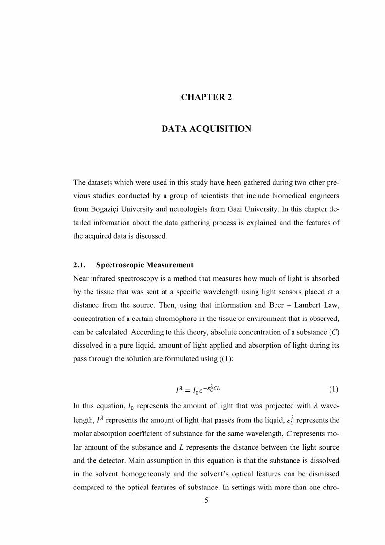
2.1. Spectroscopic Measurement

Near infrared spectroscopy is a method that measures how much of light is absorbed

by the tissue that was sent at a specific wavelength using light sensors placed at a

distance from the source. Then, using that information and Beer – Lambert Law,

concentration of a certain chromophore in the tissue or environment that is observed,

can be calculated. According to this theory, absolute concentration of a substance (C)

dissolved in a pure liquid, amount of light applied and absorption of light during its

pass through the solution are formulated using ((1):

(1)

In this equation, represents the amount of light that was projected with wave-

length, represents the amount of light that passes from the liquid, represents the

molar absorption coefficient of substance for the same wavelength, C represents mo-

lar amount of the substance and L represents the distance between the light source

and the detector. Main assumption in this equation is that the substance is dissolved

in the solvent homogeneously and the solvent’s optical features can be dismissed

compared to the optical features of substance. In settings with more than one chro-

6

mophore dissolved, the equation is modified as below, with and being molar

quantity of different chromophores:

[ (

) ] (2)

In this case, because there are two unknown parameters, a second measurement with

a different wavelength of light should be conducted and using these two equations,

separate amounts corresponding to the different chromophores can be calculated.

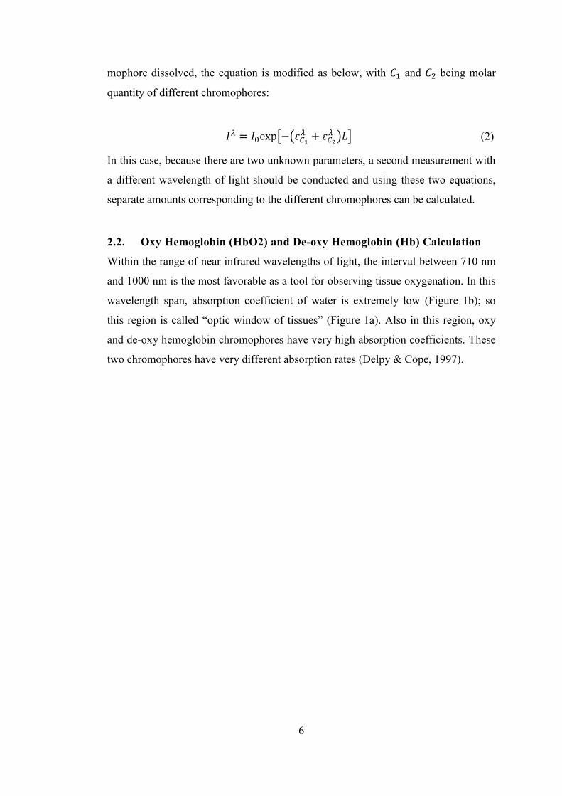
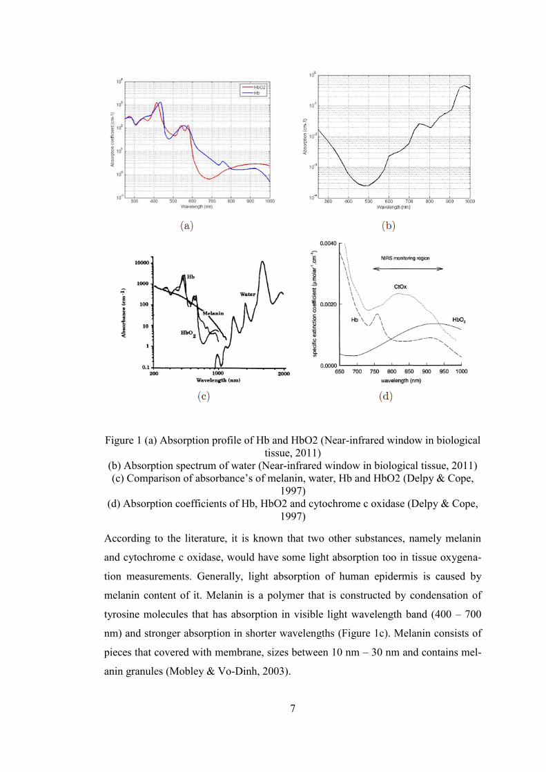
2.2. Oxy Hemoglobin (HbO2) and De-oxy Hemoglobin (Hb) Calculation

Within the range of near infrared wavelengths of light, the interval between 710 nm

and 1000 nm is the most favorable as a tool for observing tissue oxygenation. In this

wavelength span, absorption coefficient of water is extremely low (Figure 1b); so

this region is called “optic window of tissues” (Figure 1a). Also in this region, oxy

and de-oxy hemoglobin chromophores have very high absorption coefficients. These

two chromophores have very different absorption rates (Delpy & Cope, 1997).

7

Figure 1 (a) Absorption profile of Hb and HbO2 (Near-infrared window in biological

tissue, 2011)

(b) Absorption spectrum of water (Near-infrared window in biological tissue, 2011)

(c) Comparison of absorbance’s of melanin, water, Hb and HbO2 (Delpy & Cope,

1997)

(d) Absorption coefficients of Hb, HbO2 and cytochrome c oxidase (Delpy & Cope,

1997)

According to the literature, it is known that two other substances, namely melanin

and cytochrome c oxidase, would have some light absorption too in tissue oxygena-

tion measurements. Generally, light absorption of human epidermis is caused by

melanin content of it. Melanin is a polymer that is constructed by condensation of

tyrosine molecules that has absorption in visible light wavelength band (400 – 700

nm) and stronger absorption in shorter wavelengths (Figure 1c). Melanin consists of

pieces that covered with membrane, sizes between 10 nm – 30 nm and contains mel-

anin granules (Mobley & Vo-Dinh, 2003).

8

Cytochrome c oxidase is an enzyme that is used during cellular respiration. Mito-

chondria help oxygen to combine with hydrogen to build up water by giving an elec-

tron from cytochrome c oxidase to hydrogen in its membrane. Although that absorp-

tion coefficient of cytochrome c oxidase is higher than of those Hb and HbO2

(Figure 1d), for in vivo measurements, due to its low change rate of concentration

and low concentration, it has no effect (Richards-Kortum & Sevick-Muraca, 1996).

In order to calculate changes in concentration of Hb and HbO2, measurements of

light absorption conducted using two light sources with different wavelengths, can be

placed on equation below which is derived from Beer – Lambert Law (Chance,

1991) (Delpy D. T., et al., 1988) (Hoshi, 2003) (Hoshi, 2011) (Villringer & Chance,

1997).

{ }

(3)

In this equation; represents the change in ratio of light passed through to the

light projected for wavelength of ,

represents molar absorption coefficients

of different chromophores and represents the absolute change in molar

amounts of chromophores compared to the initial moment that the light was project-

ed. Since absorption coefficient of each chromophore for each wavelength of light, is

different, absorption measurements conducted with at least two light sources with

different wavelengths can result in calculation of change of Hb and HbO2 concentra-

tions as shown in the example equations below.

[ ]

(

) (4)

[ ]

(

) (5)

In these measurements, wavelengths of light that are going to be used can be selected

as and , since they should be selected above and below

the isosbestic point (specific wavelength at which two chemical species have the

9

same molar absorptivity) which is 800 nm (Figure 1a). A single distance measure

between single sensor and single light source is used in this equation.

2.3. Oxy and De-oxy Hemoglobin Measurement from Live Tissue

Blood diffusion and oxygenation of live tissue can be observed using two methods,

one is invasive and the other is non-invasive. In invasive method, amount of dis-

solved oxygen or its partial pressure (PO2) can be measured using a thin probe with

thickness of 250 µm, placed in the tissue. (Oxford Optronix, 2011)

Using non-invasive method, with light sources and sensors placed above the skin,

concentration of Hb and HbO2 contained in tissue below the skin is calculated.

Again, using an equation derived from Beer-Lambert Law, measured light data is

converted to concentration data. But, the tissue underneath the skin is not homoge-

nous as Beer-Lambert Law foresees. It is made up of several different layers. Each of

these layers has capillary vessels in them which would have independent changes in

Hb and HbO2 concentration from others. The light projected to such area, would pass

through some and would be reflected back from some. The light that is reflected back

carries data about [ ] and [ ] of all layers that it passed through. To cover

all these concerns, some changes are made on the Beer-Lambert Law given in (

(1)

) and this new law is called Modified Beer-Lambert Law. This modified law covers

these points:

1. Tissue being reflective besides being absorbent

2. Depending on the positions of light source and sensor, a new differential light

path length is suggested

3. Absorbance of chromophores in the area observed, being greater than the re-

flectivity of them. ( )

4. Changes caused by light reflection in the environment being rather too small

than of those caused by light absorption. ( )

10

Modified Beer-Lambert law which accounts for these points is given in ((6) (Delpy

D. T., et al., 1988) (Sayli, 2009) (Sayli, Aksel, & Akin, 2008).

( ) (6)

In this equation, represents the wavelength of light used, represents the opti-

cal density in this wavelength, represents the power of light sent to the tissue in

Watts, represents the power of light received back from the tissue in Watts, rep-

resents absorption coefficient specific to that wavelength in , C repre-

sents the absolute concentration of chromophore in environment in , r represents

the shortest path between light source and sensor in cm, represents differential

path length factor. Actually, is equal to divided by r. is added for the

geometry and reflection property of the area. The assumption of a change in concen-

tration of a chromophore is going to affect optical density is valid. These measure-

ments can be done with two light sources with different wavelengths and using equa-

tions in ((4) and ((5), concentration change of Hb and HbO2 can be calculated be-

tween light source and sensor.

2.4. Niroxcope

NIRS equipment that is used in both studies was developed in the Neuro-Optical

Imaging Laboratory of Biomedical Engineering Department of Boğaziçi University.

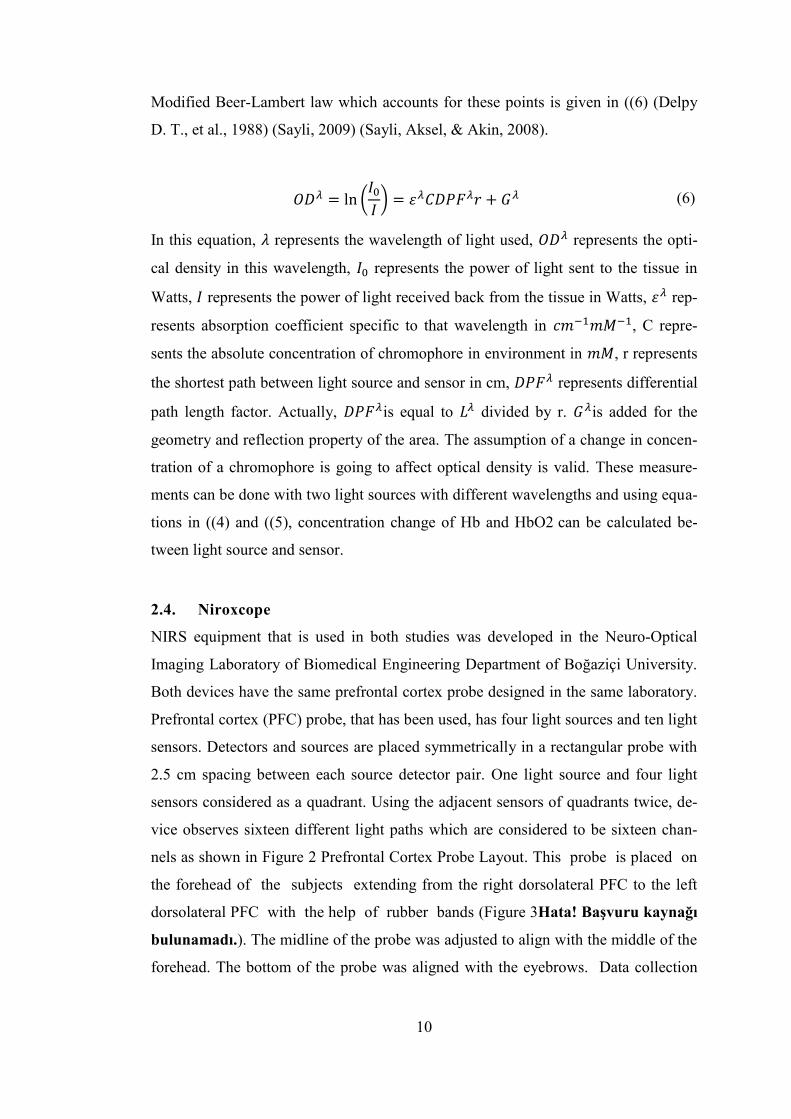
Both devices have the same prefrontal cortex probe designed in the same laboratory.

Prefrontal cortex (PFC) probe, that has been used, has four light sources and ten light

sensors. Detectors and sources are placed symmetrically in a rectangular probe with

2.5 cm spacing between each source detector pair. One light source and four light

sensors considered as a quadrant. Using the adjacent sensors of quadrants twice, de-

vice observes sixteen different light paths which are considered to be sixteen chan-

nels as shown in Figure 2 Prefrontal Cortex Probe Layout. This probe is placed on

the forehead of the subjects extending from the right dorsolateral PFC to the left

dorsolateral PFC with the help of rubber bands (Figure 3Hata! Başvuru kaynağı

bulunamadı.). The midline of the probe was adjusted to align with the middle of the

forehead. The bottom of the probe was aligned with the eyebrows. Data collection

11

started with the resting state and ended with resting state in order to observe

the baseline measurements.

S1 Light Sensor

LS1 Light Source Quadrant

Legend

C1 Light Path (Channel)

Q1

LS1

S1

S2 S4

S3

LS2

S6

S5

LS3

S8

S7

LS4

S10

S9

C1

C4

C3

C2

C5

C8

C7

C6

C9

C12

C11

C10

C13

C16

C15

C14

Q1 Q2 Q3 Q4

Figure 2 Prefrontal Cortex Probe Layout

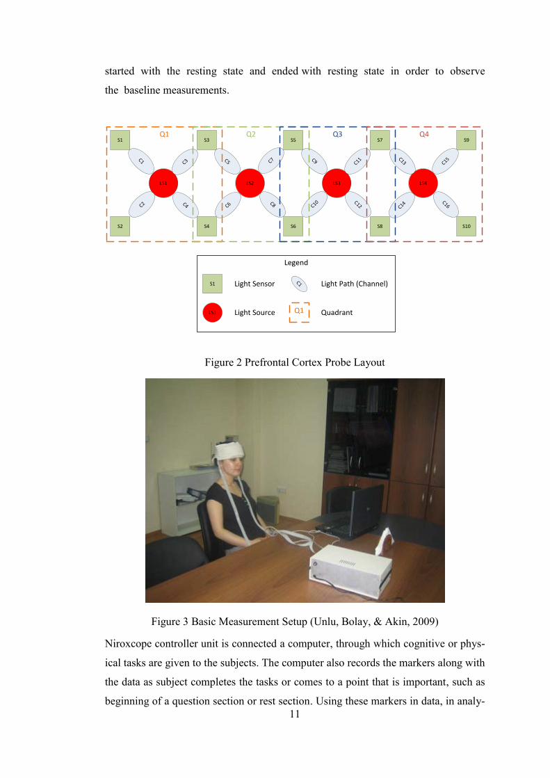
Figure 3 Basic Measurement Setup (Unlu, Bolay, & Akin, 2009)

Niroxcope controller unit is connected a computer, through which cognitive or phys-

ical tasks are given to the subjects. The computer also records the markers along with

the data as subject completes the tasks or comes to a point that is important, such as

beginning of a question section or rest section. Using these markers in data, in analy-

12

sis phase, sections of measurement (question sections, rest sections, breath hold sec-

tions etc.) can be separated. Data is recorded in a cyclic routine. It begins with first

quadrant in the probe and activates the light source of first wave length of first quad-

rant. Then records measurements acquired from the sensors of first quadrant. After

that, the second light source with second wavelength is activated and again meas-

urements of first quadrant’s sensors are recorded. After doing same routine for all

four quadrants, controller returns back to the beginning and continues with the first

quadrant again. A cycle of all four quadrants is completed in approximately 572 mil-

liseconds. Each cycle is represented as a row in data file with tab separated columns.

Each value in each cell in data file is the voltage measurement of light sensor varying

from 0 to 5 Volts.

After measurements are recorded to data files for each subject, these data files are

processed with a Matlab© based software developed by same group. This software

reads the data files and extracts marker information. After marker extraction, using

the Modified Beer-Lambert Law ((6), it converts the voltage data to HbO2, Hb and

blood volume data.

2.5. Dataset 1

First study was designed to investigate hemodynamic differences between mi-

graineur and healthy subjects during a mental arithmetic task. The task is expected to

create a cognitive burden and consequently result in a change in the blood flow in the

prefrontal cortex. Participants (5 healthy men, 11 healthy women, 4 migraineur men

and 12 migraineur women) were aged between 20 and 40 years with mean of

23.94±3.45, who had their college degree and were informed about the test procedure

before the experiment and consented. Participants who were in their menstrual peri-

od, had cardiovascular or neurologic or psychological problems, had experienced

migraine attack within previous 3 days from the experiment or had been using mi-

graine medication were kept exempt from the study. Subjects were requested to an-

swer as quickly as possible for mental arithmetic questions during three consequent

sessions which include different question groups derived from different levels. Ques-

tion sessions last for 60 seconds and had 60 seconds of rest periods in between (see

Figure 4 Timeline of first study).

13

Figure 4 Timeline of first study

Due to measurement errors such as a faulty sensor or wrong positioning of PFC

probe, there was some loss in data. Channel 15 of all data was faulty due to faulty

sensor 9 in PFC probe. Also data of 6 of migraineur subjects and 3 healthy subjects

were eliminated due to error. Total of 13 healthy and 10 migraineur data could be

used in classification trials. Reported results shows that, increase in mean values of

oxy-hemoglobin volume induced by the first level of questions in the regions of PFC

of significant 8 sensors are higher in healthy people in contrast with migraineurs

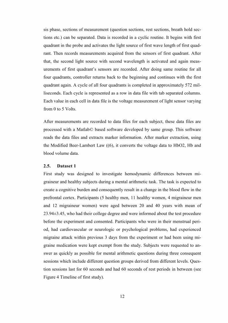
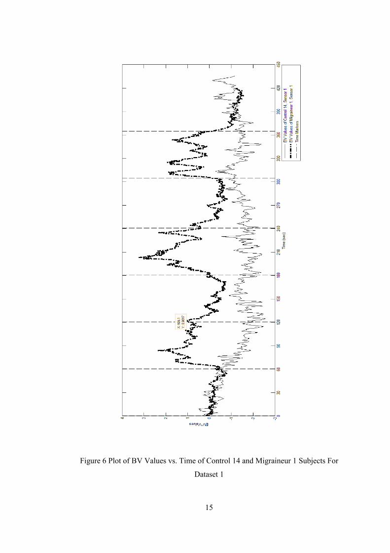
(Unlu, Bolay, & Akin, 2009). In Figure 5 Plot of HB Values vs. Time of Control 14

and Migraineur 1 Subjects For Dataset 1and Figure 6 Plot of BV Values vs. Time of

Control 14 and Migraineur 1 Subjects For Dataset 1 sample plots of BV and HB data

are shown. As their relative time markers are same along the study, both migraineur

and healthy plot sample can be shown on the same graph.

14

Figure 5 Plot of HB Values vs. Time of Control 14 and Migraineur 1 Subjects For

Dataset 1

15

Figure 6 Plot of BV Values vs. Time of Control 14 and Migraineur 1 Subjects For

Dataset 1

16

2.6. Dataset 2

Second study whose data was used seeks to observe whether there were any differ-

ences between migraineur and healthy hemodynamic metabolisms while conducting

a task which results in a physical change of PFC vascular system. Six participants

diagnosed with migraine without aura (five women with ages 29. 2 ± 9.0, one man,

age 39) according to IHS criteria and six healthy subjects (four women and two men,

with ages 26.3 ± 1.6) from the outpatient headache clinic. Participants with migraine

were not using any prophylactic medication and had not have any migraine attack in

three days period before the day that they participated in the experiment. Subjects

were positioned in supine position, and asked to breathe normally during rest peri-

ods. After an initial 60 seconds of rest, subjects were asked to exhale all the air and

hold their breaths for a minimum of 20 seconds as much as they can (usually 30 se-

conds). The procedure of breath hold was repeated four times, with a 90 seconds of

rest between each hold episode.

Figure 7 Approximate timeline for second study

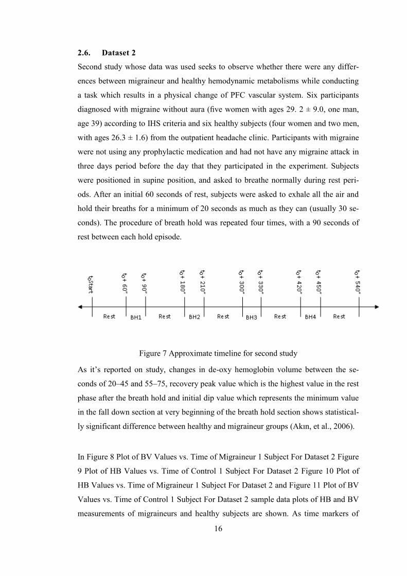
As it’s reported on study, changes in de-oxy hemoglobin volume between the se-

conds of 20–45 and 55–75, recovery peak value which is the highest value in the rest

phase after the breath hold and initial dip value which represents the minimum value

in the fall down section at very beginning of the breath hold section shows statistical-

ly significant difference between healthy and migraineur groups (Akın, et al., 2006).

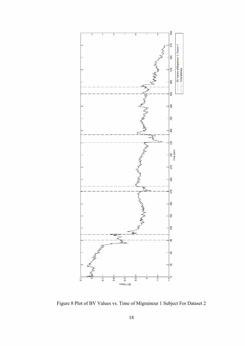
In Figure 8 Plot of BV Values vs. Time of Migraineur 1 Subject For Dataset 2 Figure

9 Plot of HB Values vs. Time of Control 1 Subject For Dataset 2 Figure 10 Plot of

HB Values vs. Time of Migraineur 1 Subject For Dataset 2 and Figure 11 Plot of BV

Values vs. Time of Control 1 Subject For Dataset 2 sample data plots of HB and BV

measurements of migraineurs and healthy subjects are shown. As time markers of

17

subjects are not same, migraineur and healthy data plots could not be shown on the

same graph.

18

Figure 8 Plot of BV Values vs. Time of Migraineur 1 Subject For Dataset 2

19

Figure 9 Plot of HB Values vs. Time of Control 1 Subject For Dataset 2

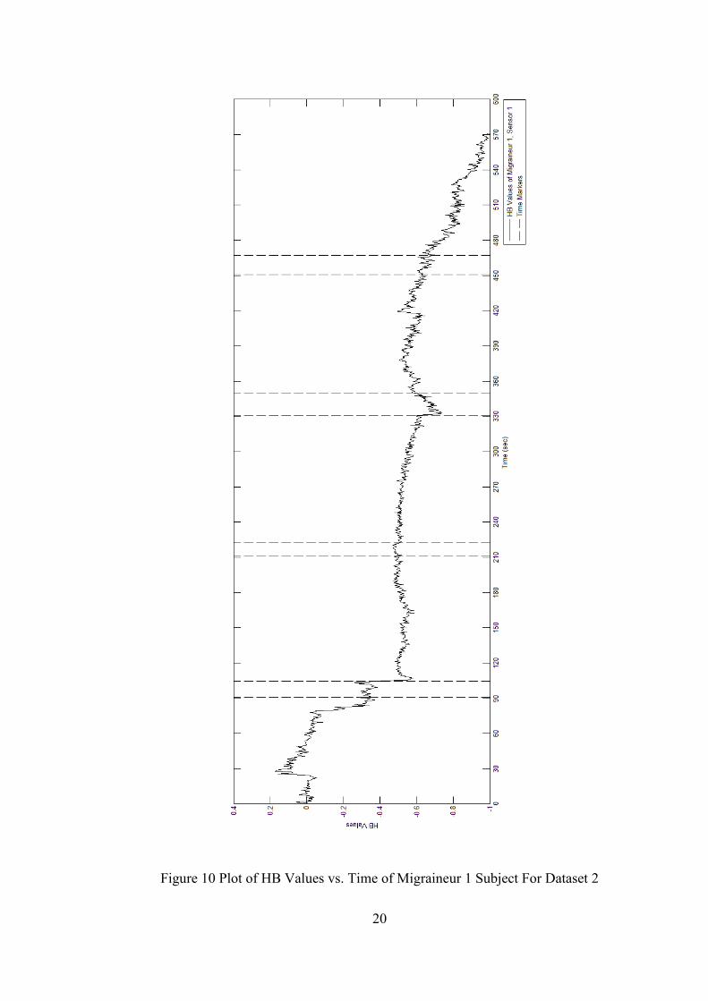
20

Figure 10 Plot of HB Values vs. Time of Migraineur 1 Subject For Dataset 2

21

Figure 11 Plot of BV Values vs. Time of Control 1 Subject For Dataset 2

22

CHAPTER 3

FEATURE EXTRACTION AND CLASSIFICATION

3.1. Feature Extraction

Both datasets have a time dependent, temporal nature so that a pre-classification task

of future extraction process should be conducted before using statistical classifiers

such as Naïve Bayes and clustering algorithms such as K-Nearest Neighbor.

In order to understand the physiological base of the experiments and their expected

consequences over the datasets measured, a neurologist was consulted as field expert.

According to the field expert; as the migraineurs are expected to be tired more than

healthy subjects, their de-oxy hemoglobin and blood volume levels are expected to

be higher at the end of the measuring approaches. Being tired means that, substances

that are produced during the work of neurons in PFC, are produced faster than the

vascular system can clean. Thus, more end-product substances such as de-oxy hemo-

globin, sodium and potassium are expected to pile up in vascular system of PFC and

surrounding tissue of migraineurs; because of different neurovascular coupling prop-

erty caused by the migraine disease. Also, it was suggested that, in addition to physi-

cal burdens to PFC, such as breath hold and head down maneuver, measurements of

BV and Hb during cognitive tasks could be discriminative for migraineurs too.

Taking these inputs in consideration, de-oxy hemoglobin and blood volume data

generated at the task sections which are closer to the end of measurement were in-

spected. To remove the time dependency, mean value for each question or breath

hold session and rest sessions before and after them are calculated for Hb and blood

volume (BV) data. Also differences between the mean value of a question or breath

23

hold session and the mean value of the rest session coming before it is also calculated

to see how much that session increased the observed property (Hb or BV).

For first study’s dataset, 3 mean values of Hb are calculated for each question ses-

sion, 3 mean values of BV are calculated for each question session, 3 mean differ-

ence values for differences between mean values of Hb in each question session and

the rest session coming before it and 3 mean difference values for differences be-

tween mean values of BV in each question session and the rest session coming be-

fore it. All these mean values are calculated for each 15 channels separately.

For the dataset collected in second study, 4 mean values of Hb are calculated for

each breath hold session, 4 mean values of BV are calculated for each breath hold

session, 4 mean difference values for differences between mean values of Hb in each

breath hold session and the rest session coming before it and 4 mean difference val-

ues for differences between mean values of BV in each breath hold session and the

rest session coming before it.

3.2. Classification

With features extracted from temporal datasets, a classification and a clustering algo-

rithm were utilized in classification task, namely Naïve Bayes (NB) and K Nearest

Neighbor (KNN). These algorithms were selected because minimum error rate nature

of NB. Also, as the labels of measurements in training and test sets were known, this

learning method is an example of supervised learning and NB is shown to be work-

ing very well in real world problems with supervised learning (Zhang, 2004). In clas-

sification trials, as both datasets are small in terms of number of subjects, separating

random training and test sets and doing n-fold trials was not viable. Instead, leave-

one-out method was implemented (Furey, et al., 2000). In each trial, one of the sub-

jects was left out and classification or clustering algorithm was trained with the re-

maining; then the measurement that was left out, used as test subject.

Our literature survey revealed that there are only a limited number of classification

studies that use oxy and de-oxy hemoglobin data acquired with fNIRS as input is

available. In 2006, Sitaram et al. (2007) reported findings of a classification trial us-

24

ing fNIRS data that was gathered from 5 healthy subjects during repeated right-hand

and left-hand motor imagery tasks. This data was fed into two different pattern clas-

sification methods namely Support Vector Machine (SVM) and Hidden Markov

Model (HMM). The study was conducted in order to investigate the possibility of a

brain computer interface (BCI) using NIRS measurements. But study was conducted

only using data from healthy subjects and data of subjects classified among each oth-

er. Aim of the classification was to differentiate right hand imagery from left hand

imagery data of the same subject. As a result, NIRS was found suitable for develop-

ment of an online BCI in consistency with pattern classification methods (Sitaram, et

al., 2007). As their dataset was big enough thanks to repeated measurements, it was

possible to use pattern classification methods such as HMM and SVM. Unfortunate-

ly, with small datasets such as dataset 1 and dataset 2, it is not possible to do so.

Naïve Bayes is a pattern classification technique that has been used since the very

beginning of classification trials which is based on Bayes’ Theorem. It considers

both a priori probability (P(wj), probability of w being an example of class j) and

likelihood (p(x|wj), probability of w being an example of class j depending on x fea-

ture) of a test subject belonging in to a class. According to Bayes’ rule;

(7)

Naïve Bayes classifier simply calculates posterior probabilities using prior probabili-

ties and a likelihood probability derived from the training set, and then assigns the

label of the class that has the biggest posterior probability, to the test subject. Likeli-

hood of a subject belonging to a class depending on a value of a feature is simply

calculated with the distribution function of that feature (Duda, Hart, & Stork, 2000).

It is known that features that are dependent to each other lower performance of Naïve

Bayes classifier. To make sure that, this problem is not affecting our case, we con-

sulted to the field expert who informed us that there is no evidence that the physical

locations that measurements were taken are dependent to each other. There is no pri-

or evidence that shows dependency between hemodynamic properties of regions in

25

prefrontal cortex. Thus, it is assumed that there are no dependency between features

in trials.

KNN classifier selects a class label for a test sample according to the label of the k

nearest neighbor of that test sample in feature space. The class that has higher num-

ber of neighbors to the test sample wins against others (Duda, Hart, & Stork, 2000).

As there are many features extracted from dataset, their importance in classification

is unknown except field expert information provided. In order to prevent errors

caused by “curse of dimensionality”, a dimension reduction algorithm, principal

component analysis (PCA) has been used and all of classifiers and feature sets have

been merged in trials with and without PCA. PCA is a method that investigates each

feature distribution provided in the training set and tries to find out the most correlat-

ed ones within the classes. Ordering features according to their correlation from high

to low, allows the user find out features’ importance for the classification task.

(Duda, Hart, & Stork, 2000)

For classification tasks, NB classifier and PCA software provided in statistics

toolbox library and KNN classifier provided in bioinformatics toolbox library, by

Matlab©, have been utilized. Both classifiers were used with default parameters as

there were no prior experiences with classification of NIRS data using these classifi-

ers and their most common application parameters were set as default. NB classifier

was used with Gaussian distribution and empirical prior probability estimation which

derives a priori probabilities from the training set. KNN classifier was used with Eu-

clidian distance measure and label of the nearest neighbor was selected as tie break-

er.

All classification trials were repeated in three different sessions in order to eliminate

the possibility of random error and results have been assured to be the same for all

trials. Predictions of classifiers in each trial were same with the other two.

After feature extraction, extracted feature sets were used both separately and together

in classification trials. For example, in classification of data set acquired from first

26

study, means of blood volume changes in question level 1 recorded from 15 channels

were fed to the classifiers as a single dataset. Also all these mean values of BV and

Hb in all question levels from 15 channels were merged as a dataset with 90 features

and classifiers were run on that dataset too. Same is done with dataset collected dur-

ing second study and mean difference values. Also, the k value of KNN classifier

was changed from 1 to 10 and for all these trials, each k value from 1 to 10 was tried.

For each feature set, the k value with best success ratio will be reported. In addition

to that, PCA was applied to all feature sets, and classifiers were tried with this da-

tasets too. All trials repeated for each number of features. For example, again with

the example above, PCA applied to the dataset data for 14 times each time reducing

it to 1 less feature 14 features to 1 and classification was tried 14 times. Results of

all these trials are going to be reported in this document.

In classification trials of both datasets,

for each subject’s data

for each feature set,

for each classifier (with and without PCA),

for each k value from 1 to 10

And for each number of features after PCA from 1 to 14

a trial has been completed.

For the dataset 1, 15 channels, 12 feature sets, 2 classifiers and 23 subjects are pre-

sent. A total of 91080 classification trials with different settings and/or different fea-

ture sets have been completed for three times. For dataset 2, 16 channels, 16 feature

sets, 2 classifiers and 12 subjects are present. A total of 67584 classification trials

with different settings and/or different feature sets have been completed for three

times.

27

CHAPTER 4

RESULTS AND COMPARISON OF TRIALS

As mentioned in previous chapter, more than 150 000 trials have been completed,

and for each dataset and each classification method, result and settings of the trial

with highest success ratio is reported. Number of features used after PCA and k value

for KNN of the trial with the best performance is reported for each classifier and fea-

ture set. The following metrics are calculated and presented:

True positive (TP, number of migraineur subjects classified as migraineur by

classifier),

False positive (FP, number of healthy subjects classified as migraineur by

classifier),

True negative (TN, number of healthy subjects classified as healthy by classi-

fier)

And false negative (FN, number of migraineur subjects classified as healthy

by classifier)

Sensitivity (ratio of correctly classified migraineurs to the total number of

migraineurs)

Specificity (ratio of correctly classified healthy to the subjects that are classi-

fied as healthy)

Success ratio values (ratio of correct classifications to the total number of

subjects) are reported below for each dataset and classifier.

Precision (ratio of correctly classified migraineurs to the subjects that are

classified as migraineurs).

28

Abbreviations used in result reports are;

NB for Naïve Bayes classifier

kNN for k-nearest neighbor classifier with k varying from 1 to 10

wPCA for with PCA applied

nF for n features used in trial.

For all result tables, cell with the maximum value for each column, is printed in red.

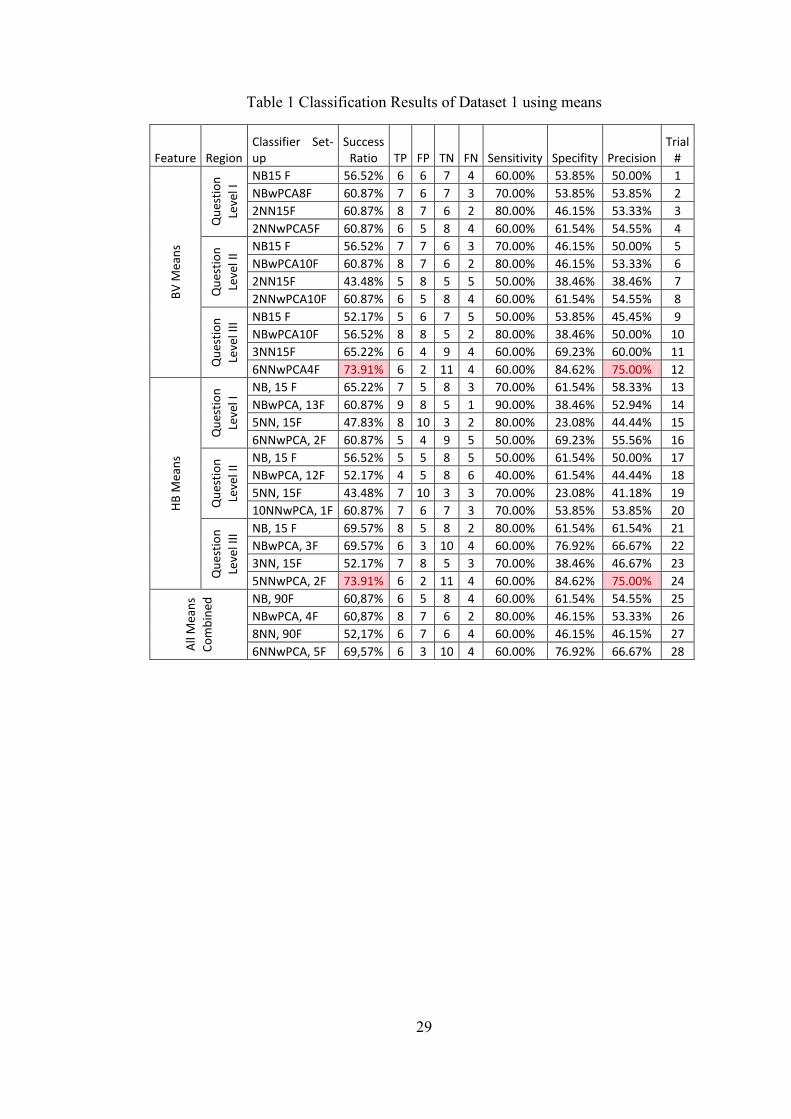
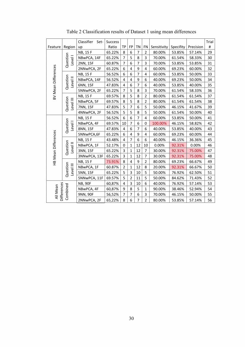
4.1. Classification Results of Dataset 1

Classification results of dataset 1 are summarized in Table 1 Classification Results of

Dataset 1 using means and Table 2. In these tables, calculated feature from original

dataset is given in “Feature” column, observed region of the experiment is given in

“Region” column, classifier, feature reduction method (if used), number of features

observed are given in “Classifier Setting” column, success ratio calculated as per-

centage of truly classified is given in “Success Ratio” column and true positive, false

positive, true negative and false negative values are given in the rest of the table.

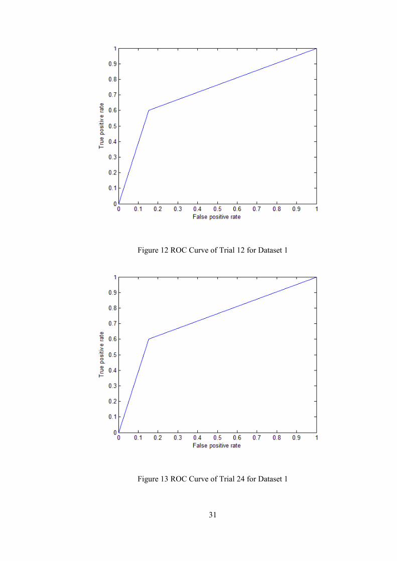
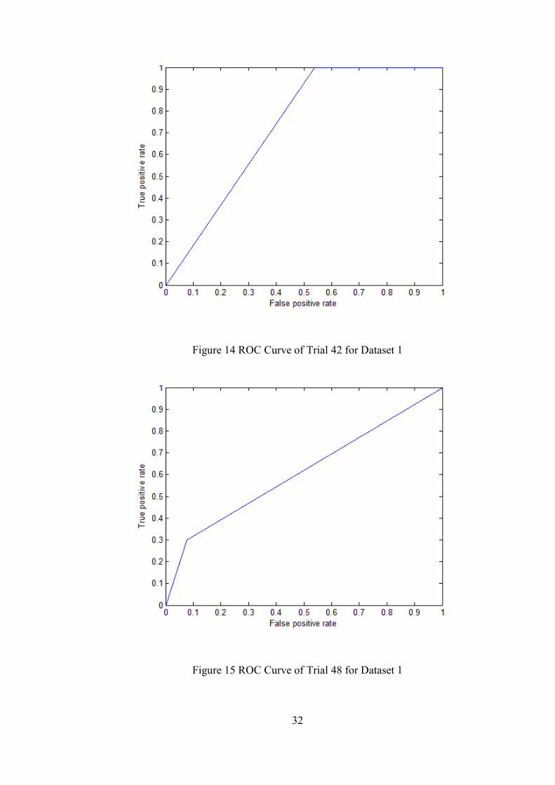
Highest success rate was found as 73.91% with features acquired from question level

III region of the experiment data. ROC curves of trials that have highest success ra-

tio, highest sensitivity and highest specificity values are given in Figure 12 ROC

Curve of Trial 12 for Dataset 1, Figure 13 ROC Curve of Trial 24 for Dataset 1 Fig-

ure 14 ROC Curve of Trial 42 for Dataset 1 and Figure 15 ROC Curve of Trial 48 for

Dataset 1.

29

Table 1 Classification Results of Dataset 1 using means

Feature Region Classifier Set-up

Success Ratio TP FP TN FN Sensitivity Specifity Precision

Trial #

BV

Mea

ns

Qu

esti

on

Leve

l I NB15 F 56.52% 6 6 7 4 60.00% 53.85% 50.00% 1

NBwPCA8F 60.87% 7 6 7 3 70.00% 53.85% 53.85% 2

2NN15F 60.87% 8 7 6 2 80.00% 46.15% 53.33% 3

2NNwPCA5F 60.87% 6 5 8 4 60.00% 61.54% 54.55% 4 Q

ues

tio

n

Leve

l II NB15 F 56.52% 7 7 6 3 70.00% 46.15% 50.00% 5

NBwPCA10F 60.87% 8 7 6 2 80.00% 46.15% 53.33% 6

2NN15F 43.48% 5 8 5 5 50.00% 38.46% 38.46% 7

2NNwPCA10F 60.87% 6 5 8 4 60.00% 61.54% 54.55% 8

Qu

esti

on

Leve

l III

NB15 F 52.17% 5 6 7 5 50.00% 53.85% 45.45% 9

NBwPCA10F 56.52% 8 8 5 2 80.00% 38.46% 50.00% 10

3NN15F 65.22% 6 4 9 4 60.00% 69.23% 60.00% 11

6NNwPCA4F 73.91% 6 2 11 4 60.00% 84.62% 75.00% 12

HB

Mea

ns

Qu

esti

on

Leve

l I NB, 15 F 65.22% 7 5 8 3 70.00% 61.54% 58.33% 13

NBwPCA, 13F 60.87% 9 8 5 1 90.00% 38.46% 52.94% 14

5NN, 15F 47.83% 8 10 3 2 80.00% 23.08% 44.44% 15

6NNwPCA, 2F 60.87% 5 4 9 5 50.00% 69.23% 55.56% 16

Qu

esti

on

Leve

l II NB, 15 F 56.52% 5 5 8 5 50.00% 61.54% 50.00% 17

NBwPCA, 12F 52.17% 4 5 8 6 40.00% 61.54% 44.44% 18

5NN, 15F 43.48% 7 10 3 3 70.00% 23.08% 41.18% 19

10NNwPCA, 1F 60.87% 7 6 7 3 70.00% 53.85% 53.85% 20

Qu

esti

on

Leve

l III

NB, 15 F 69.57% 8 5 8 2 80.00% 61.54% 61.54% 21

NBwPCA, 3F 69.57% 6 3 10 4 60.00% 76.92% 66.67% 22

3NN, 15F 52.17% 7 8 5 3 70.00% 38.46% 46.67% 23

5NNwPCA, 2F 73.91% 6 2 11 4 60.00% 84.62% 75.00% 24

All

Mea

ns

Co

mb

ined

NB, 90F 60,87% 6 5 8 4 60.00% 61.54% 54.55% 25

NBwPCA, 4F 60,87% 8 7 6 2 80.00% 46.15% 53.33% 26

8NN, 90F 52,17% 6 7 6 4 60.00% 46.15% 46.15% 27

6NNwPCA, 5F 69,57% 6 3 10 4 60.00% 76.92% 66.67% 28

30

Table 2 Classification results of Dataset 1 using mean differences

Feature Region Classifier Set-up

Success Ratio TP FP TN FN Sensitivity Specifity Precision

Trial #

BV

Mea

n D

iffe

ren

ces Qu

esti

on

Leve

l I NB, 15 F 65.22% 8 6 7 2 80.00% 53.85% 57.14% 29

NBwPCA, 14F 65.22% 7 5 8 3 70.00% 61.54% 58.33% 30

2NN, 15F 60.87% 7 6 7 3 70.00% 53.85% 53.85% 31

2NNwPCA, 2F 65.22% 6 4 9 4 60.00% 69.23% 60.00% 32 Q

ues

tio

n

Leve

l II NB, 15 F 56.52% 6 6 7 4 60.00% 53.85% 50.00% 33

NBwPCA, 14F 56.52% 4 4 9 6 40.00% 69.23% 50.00% 34

6NN, 15F 47.83% 4 6 7 6 40.00% 53.85% 40.00% 35

5NNwPCA, 2F 65.22% 7 5 8 3 70.00% 61.54% 58.33% 36

Qu

esti

on

Leve

l III

NB, 15 F 69.57% 8 5 8 2 80.00% 61.54% 61.54% 37

NBwPCA, 5F 69.57% 8 5 8 2 80.00% 61.54% 61.54% 38

7NN, 15F 47.83% 5 7 6 5 50.00% 46.15% 41.67% 39

4NNwPCA, 2F 56.52% 5 5 8 5 50.00% 61.54% 50.00% 40

HB

Mea

n D

iffe

ren

ces Qu

esti

on

Leve

l I NB, 15 F 56.52% 6 6 7 4 60.00% 53.85% 50.00% 41

NBwPCA, 4F 69.57% 10 7 6 0 100.00% 46.15% 58.82% 42

8NN, 15F 47.83% 4 6 7 6 40.00% 53.85% 40.00% 43

5NNwPCA,6F 65.22% 6 4 9 4 60.00% 69.23% 60.00% 44

Qu

esti

on

Leve

l II NB, 15 F 43.48% 4 7 6 6 40.00% 46.15% 36.36% 45

NBwPCA, 1F 52.17% 0 1 12 10 0.00% 92.31% 0.00% 46

3NN, 15F 65.22% 3 1 12 7 30.00% 92.31% 75.00% 47

3NNwPCA, 13F 65.22% 3 1 12 7 30.00% 92.31% 75.00% 48

Qu

esti

on

Leve

l III

NB, 15 F 73.91% 8 4 9 2 80.00% 69.23% 66.67% 49

NBwPCA, 1F 60.87% 2 1 12 8 20.00% 92.31% 66.67% 50

5NN, 15F 65.22% 5 3 10 5 50.00% 76.92% 62.50% 51

5NNwPCA, 11F 69.57% 5 2 11 5 50.00% 84.62% 71.43% 52

All

Mea

n

Dif

fere

nce

s

Co

mb

ined

NB, 90F 60,87% 4 3 10 6 40.00% 76.92% 57.14% 53

NBwPCA, 4F 60,87% 9 8 5 1 90.00% 38.46% 52.94% 54

9NN, 90F 56,52% 7 7 6 3 70.00% 46.15% 50.00% 55

2NNwPCA, 2F 65,22% 8 6 7 2 80.00% 53.85% 57.14% 56

31

Figure 12 ROC Curve of Trial 12 for Dataset 1


32



33

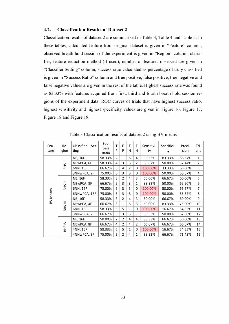
4.2. Classification Results of Dataset 2

Classification results of dataset 2 are summarized in Table 3, Table 4 and Table 5. In

these tables, calculated feature from original dataset is given in “Feature” column,

observed breath hold session of the experiment is given in “Region” column, classi-

fier, feature reduction method (if used), number of features observed are given in

“Classifier Setting” column, success ratio calculated as percentage of truly classified

is given in “Success Ratio” column and true positive, false positive, true negative and

false negative values are given in the rest of the table. Highest success rate was found

as 83.33% with features acquired from first, third and fourth breath hold session re-

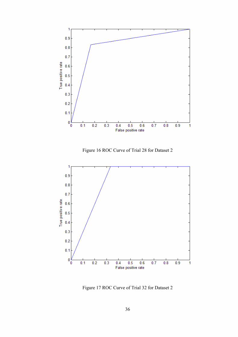
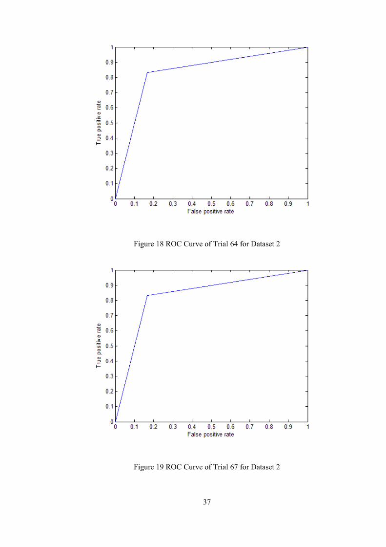
gions of the experiment data. ROC curves of trials that have highest success ratio,

highest sensitivity and highest specificity values are given in Figure 16, Figure 17,

Figure 18 and Figure 19.

Table 3 Classification results of dataset 2 using BV means

Fea-ture

Re-gion

Classifier Set-ting

Suc-cess Ratio

TP

FP

TN

FN

Sensitivi-ty

Specifici-ty

Preci-sion

Tri-al #

BV

Mea

ns

BH

S I

NB, 16F 58.33% 2 1 5 4 33.33% 83.33% 66.67% 1

NBwPCA, 6F 58.33% 4 3 3 2 66.67% 50.00% 57.14% 2

6NN, 16F 66.67% 6 4 2 0 100.00% 33.33% 60.00% 3

3NNwPCA, 2F 75.00% 6 3 3 0 100.00% 50.00% 66.67% 4

BH

S II

NB, 16F 58.33% 3 2 4 3 50.00% 66.67% 60.00% 5

NBwPCA, 8F 66.67% 5 3 3 1 83.33% 50.00% 62.50% 6

6NN, 16F 75.00% 6 3 3 0 100.00% 50.00% 66.67% 7

6NNwPCA, 16F 75.00% 6 3 3 0 100.00% 50.00% 66.67% 8

BH

S II

I

NB, 16F 58.33% 3 2 4 3 50.00% 66.67% 60.00% 9

NBwPCA, 4F 66.67% 3 1 5 3 50.00% 83.33% 75.00% 10

6NN, 16F 58.33% 6 5 1 0 100.00% 16.67% 54.55% 11

3NNwPCA, 2F 66.67% 5 3 3 1 83.33% 50.00% 62.50% 12

BH

S IV

NB, 16F 50.00% 2 2 4 4 33.33% 66.67% 50.00% 13

NBwPCA, 8F 66.67% 4 2 4 2 66.67% 66.67% 66.67% 14

4NN, 16F 58.33% 6 5 1 0 100.00% 16.67% 54.55% 15

4NNwPCA, 3F 75.00% 5 2 4 1 83.33% 66.67% 71.43% 16

34

Table 4 Classification results of dataset 2 using Hb means, all means combined and

all mean differences combined

Fea-ture

Re-gion

Classifier Set-ting

Suc-cess Ratio

TP

FP

TN

FN

Sensitivi-ty

Specifici-ty

Preci-sion

Tri-al #

Hb

Mea

ns

BH

S I

NB, 16F 58.33% 4 3 3 2 66.67% 50.00% 57.14% 17

NBwPCA, 8F 66.67% 5 3 3 1 83.33% 50.00% 62.50% 18

4NN, 16F 66.67% 6 4 2 0 100.00% 33.33% 60.00% 19

4NNwPCA, 16F 66.67% 6 4 2 0 100.00% 33.33% 60.00% 20

BH

S II

NB, 16F 50.00% 4 4 2 2 66.67% 33.33% 50.00% 21

NBwPCA, 2F 66.67% 4 2 4 2 66.67% 66.67% 66.67% 22

8NN, 16F 58.33% 5 4 2 1 83.33% 33.33% 55.56% 23

8NNwPCA, 8F 66.67% 6 4 2 0 100.00% 33.33% 60.00% 24

BH

S II

I

NB, 16F 58.33% 4 3 3 2 66.67% 50.00% 57.14% 25

NBwPCA, 9F 66.67% 3 1 5 3 50.00% 83.33% 75.00% 26

8NN, 16F 66.67% 6 4 2 0 100.00% 33.33% 60.00% 27

3NNwPCA, 1F 83.33% 5 1 5 1 83.33% 83.33% 83.33% 28

BH

S IV

NB, 16F 50.00% 3 3 3 3 50.00% 50.00% 50.00% 29

NBwPCA, 2F 66.67% 4 2 4 2 66.67% 66.67% 66.67% 30

6NN, 16F 66.67% 6 4 2 0 100.00% 33.33% 60.00% 31

2NNwPCA, 3F 83.33% 6 2 4 0 100.00% 66.67% 75.00% 32

All

Mea

ns

Co

m-

bin

ed

NB, 128F 66.67% 4 2 4 2 66.67% 66.67% 66.67% 33

NBwPCA, 8F 75.00% 6 3 3 0 100.00% 50.00% 66.67% 34

6NN, 128F 75.00% 6 3 3 0 100.00% 50.00% 66.67% 35

2NNwPCA, 128F

75.00% 6 3 3 0 100.00% 50.00% 66.67% 36

All

Mea

nd

Dif

fere

nce

s

Co

mb

ined

NB, 128F 66.67% 3 1 5 3 50.00% 83.33% 75.00% 69

NBwPCA, 8F 66.67% 5 3 3 1 83.33% 50.00% 62.50% 70

3NN, 128F 66.67% 6 4 2 0 100.00% 33.33% 60.00% 71

3NNwPCA, 3F 83.33% 5 1 5 1 83.33% 83.33% 83.33% 72

35

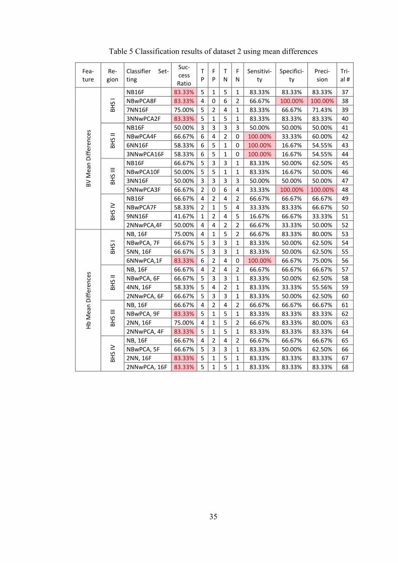
Table 5 Classification results of dataset 2 using mean differences

Fea-ture

Re-gion

Classifier Set-ting

Suc-cess Ratio

TP

FP

TN

FN

Sensitivi-ty

Specifici-ty

Preci-sion

Tri-al #

BV

Mea

n D

iffe

ren

ces

BH

S I

NB16F 83.33% 5 1 5 1 83.33% 83.33% 83.33% 37

NBwPCA8F 83.33% 4 0 6 2 66.67% 100.00% 100.00% 38

7NN16F 75.00% 5 2 4 1 83.33% 66.67% 71.43% 39

3NNwPCA2F 83.33% 5 1 5 1 83.33% 83.33% 83.33% 40 B

HS

II NB16F 50.00% 3 3 3 3 50.00% 50.00% 50.00% 41

NBwPCA4F 66.67% 6 4 2 0 100.00% 33.33% 60.00% 42

6NN16F 58.33% 6 5 1 0 100.00% 16.67% 54.55% 43

3NNwPCA16F 58.33% 6 5 1 0 100.00% 16.67% 54.55% 44

BH

S II

I

NB16F 66.67% 5 3 3 1 83.33% 50.00% 62.50% 45

NBwPCA10F 50.00% 5 5 1 1 83.33% 16.67% 50.00% 46

3NN16F 50.00% 3 3 3 3 50.00% 50.00% 50.00% 47

5NNwPCA3F 66.67% 2 0 6 4 33.33% 100.00% 100.00% 48

BH

S IV

NB16F 66.67% 4 2 4 2 66.67% 66.67% 66.67% 49

NBwPCA7F 58.33% 2 1 5 4 33.33% 83.33% 66.67% 50

9NN16F 41.67% 1 2 4 5 16.67% 66.67% 33.33% 51

2NNwPCA,4F 50.00% 4 4 2 2 66.67% 33.33% 50.00% 52

Hb

Mea

n D

iffe

ren

ces

BH

S I

NB, 16F 75.00% 4 1 5 2 66.67% 83.33% 80.00% 53

NBwPCA, 7F 66.67% 5 3 3 1 83.33% 50.00% 62.50% 54

5NN, 16F 66.67% 5 3 3 1 83.33% 50.00% 62.50% 55

6NNwPCA,1F 83.33% 6 2 4 0 100.00% 66.67% 75.00% 56

BH

S II

NB, 16F 66.67% 4 2 4 2 66.67% 66.67% 66.67% 57

NBwPCA, 6F 66.67% 5 3 3 1 83.33% 50.00% 62.50% 58

4NN, 16F 58.33% 5 4 2 1 83.33% 33.33% 55.56% 59

2NNwPCA, 6F 66.67% 5 3 3 1 83.33% 50.00% 62.50% 60

BH

S II

I

NB, 16F 66.67% 4 2 4 2 66.67% 66.67% 66.67% 61

NBwPCA, 9F 83.33% 5 1 5 1 83.33% 83.33% 83.33% 62

2NN, 16F 75.00% 4 1 5 2 66.67% 83.33% 80.00% 63

2NNwPCA, 4F 83.33% 5 1 5 1 83.33% 83.33% 83.33% 64

BH

S IV

NB, 16F 66.67% 4 2 4 2 66.67% 66.67% 66.67% 65

NBwPCA, 5F 66.67% 5 3 3 1 83.33% 50.00% 62.50% 66

2NN, 16F 83.33% 5 1 5 1 83.33% 83.33% 83.33% 67

2NNwPCA, 16F 83.33% 5 1 5 1 83.33% 83.33% 83.33% 68

36



37



38

Classification results are consistent with the information obtained from the field ex-

pert. Regions at the end of the experiment (third for the dataset 1 and fourth for the

dataset 2) are observed to be more significantly correlated within the groups. Thus,

classification trials using the features gathered from these regions have higher suc-

cess ratio than the trials with features extracted from the first and second regions of

the experiments.

4.3. Statistical Hypothesis Tests

In order to observe if the differences between the results are statistically significant,

statistical comparison tests should be conducted. As feature sets are extracted from

the same measurement dataset, all trials are statistically related. The ANOVA test is

a commonly used statistical method investigating if differences between more than

two related sample means are significantly different. In our case, as data is non-

parametric and binary, ANOVA’s non-parametric equivalent for binary data is

Cochran Q test (Looney, 1988). Cochran Q test was applied to the results gathered

from classification trials of both datasets separately to see whether trials succeeded

differently and also whether they classified the subjects differently, with null hypoth-

esis of there were no difference between classification trials. To calculate this statis-

tics, a table for performance of test trials and test subjects has been tabulated. In this

table columns include test trials and rows include test subjects. If a test trial predicted

the class of a subject, 1 is written as value of the cell in conjunction between row of

that subject and column of that test trial, else 0 is written. After table is constructed,

Cochran Q test statistics is calculated using the ((8). In this equation, Cj represents

the total of values in the column for the trial j, k represents number of classification

trials, Ri represents the total of values in the row i and n indicates number of test sub-

jects. If test calculated test statistic value is smaller than the (1 − α)-quintile of the

chi-squared distribution with k − 1 degrees of freedom, null hypothesis is accepted;

else it is rejected. (Alpar, 2006).

[ ∑

(∑ )

]

∑ ∑

(8)

For investigation of difference between two related samples with binary data, Mc

Nemar’s test is used (Dietterich, 1998) (Alpar, 2006). Also, to confirm results of

39

Cochran Q that there were no differences or to find out if there were differences,

which two trials were different, McNemar’s test was used, with null hypothesis of

there were no difference between subjects. To calculate Mc Nemar’s test statistics a

table with 2 rows and 2 columns is constructed, in first cell, number of test subjects

classified correctly by both methods (a) is written, in second cell, number of test sub-

jects that are classified correctly by first trial but not by the second (b) is written, in

third cell, the number of test subjects that are classified correctly by second trial but

not by the first (c) is written and to the last cell, number of test subjects that are clas-

sified wrong by both methods (d) is written. After the table creation, Mc Nemar’s

test statistics is calculated, with the ((9):

(9)

If test calculated test statistic value is smaller than the (1 − α)-quintile of the chi-

squared distribution with 1 degree of freedom, null hypothesis is accepted; else it is

rejected.

4.4. Statistical Inspection of Classification Results of Dataset 1

To apply Cochran Q analysis on classification results of dataset 1, test statistics cal-

culated using the ((8) is 34.53, smaller than the calculated chi-square distribution

statistics, 74. Thus null hypothesis is accepted; there was no statistically significant

difference in performances of trials with the confidence interval of 95%. All the trials

performed equally successful within the given dataset. But there were statistically

significant differences in predictions of classification trials for the subjects, again

with the confidence interval of 95%. Using the ((8), calculated Cochran Q statistic is

136.73 and greater than the 0.05-quintile of the chi-squared distribution with 55 de-

grees of freedom, 74. So, null hypothesis is rejected; there is statistically significant

difference between the predictions of trials for the test subjects. That means some of

the trials, labeled some of the subjects different than others.

To confirm the Cochran Q test results and find difference between the trials, pairwise

Mc Nemar’s tests are applied for the trials. Using ((9), Mc Nemar’s test statistic is

calculated for each trial pair. All of the calculated statistics using the performance

40

values of the trials were less than the 0.05-quintile of the chi-squared distribution

with 1 degree of freedom, which is 3.841. So all null hypothesis are accepted, there

were no differences in performance between trial pairs. In Cochran Q test conducted

using the predictions of trials, there was a significant difference in some of the trials.

To find out which pairs were different than each other, pairwise Mc Nemar’s tests

are conducted using the prediction data. Some of these Mc Nemar’s test statistics

were higher than the 0.05-quintile of the chi-squared distribution with 1 degree of

freedom, which is 3.841; consistent with Cochran Q test result. A total of 3080 Mc

Nemar’s tests are conducted for the performances.

As there was no significant difference between the performance measures of the tests

by the Cochran Q test, a success measure was created using the Mc Nemar’s test

results and success ratios of the test trials. Trials were inspected pairwise and for

each test pair, if their predictions were found statistically different from each other,

the trial with higher success ratio was given 1 point. As a result of this work, best

classification trial was found as the one done with blood volume means of the third

question level section as feature set and 6 nearest neighbor classifier after PCA with

4 features. Its predictions were different than 6 trials with lower success ratio and its

success ratio was 73.91%.

Consistent with the information gathered from the field expert, blood volume infor-

mation content of the regions at the end of the experiment regarding the classification

of migraineur and healthy is higher than the feature sets.

4.5. Statistical Inspection of Classification Results of Dataset 2

To apply Cochran Q analysis on classification results of dataset 2, test statistics cal-

culated using the ((8) is 46.82, smaller than the 0.05-quintile of the chi-squared dis-

tribution with 71 degrees of freedom, 93. Thus null hypothesis is accepted; there was

no statistically significant difference in performances of trials with the confidence

interval of 95%. All the trials performed equally successful within the given dataset.

But there were statistically significant differences in predictions of classification tri-

als for the subjects, again with the confidence interval of 95%. Using the ((8), calcu-

lated Cochran Q statistic is 153.74 and greater than the 0.05-quintile of the chi-

41

squared distribution with 71 degrees of freedom, 93. So, null hypothesis is rejected;

there is statistically significant difference between the predictions of trials for the test

subjects. That means some of the trials, labeled some of the subjects different than

others.

To confirm the Cochran Q test results and find difference between the trials, pairwise

Mc Nemar’s tests are applied for the trials. Using ((9), Mc Nemar’s test statistic is

calculated for each trial pair. All of the calculated statistics using the performance

values of the trials were less than the 0.05-quintile of the chi-squared distribution

with 1 degree of freedom, which is 3.841. So all null hypothesis are accepted, there

were no differences in performance between trial pairs. In Cochran Q test conducted

using the predictions of trials, there was a significant difference in some of the trials.

To find out which pairs were different than each other, pairwise Mc Nemar’s tests

are conducted using the prediction data. Some of these Mc Nemar’s test statistics

were higher than the 0.05-quintile of the chi-squared distribution with 1 degree of

freedom, which is 3.841; consistent with Cochran Q test result. A total of 5112 Mc

Nemar’s tests are conducted for the performances.

As there was no significant difference found between the performance measures of

the tests by the Cochran Q test, a success measure was created using the Mc Nemar’s

test results and success ratios of the test trials. Trials were inspected pairwise and for

each test pair, if their predictions were found statistically different from each other,

the trial with higher success ratio was given 1 point. As a result of this work, best

classification trial was found as the one done with de-oxy hemoglobin means of the

fourth breath hold section as feature set and 2 nearest neighbor classifier after PCA

with 3 features. Its predictions were different than 7 trials with lower success ratio

and its success ratio was 83.33%.

42

CHAPTER 5

CONCLUSIONS AND FUTURE WORK

5.1. Discussion

From the beginning of the study, there was a certain degree of uncertainty in which

features to extract and which classification methods to use as there were no previous

work on classification of migraineurs with neurovascular system data gathered dur-

ing cognitive or physical challenges using NIRS. This fog of unknown has been

eliminated in part thanks to the information supplied by field expert. After extracting

features in consistency with the information supplied by the field expert, extraction

methods were selected as a set of most commonly used supervised learning tech-

niques with data having unknown distribution.

Results gathered indicate significance of blood volume and de-oxy hemoglobin data

acquired in the last sessions of experiment, in classification of migraineur and

healthy from each other, in consistence with the reported expectations of the field

expert. As it was also suggested, data gathered during a cognitive task, mental arith-

metic, seems to be as successful as physical tasks.

As observed from the results of statistical tests, there is no significant difference be-

tween performance measures of the trials for both datasets. Thus, trial with better

success ratio, sensitivity and specificity would be considered as a better classification

method for migraine disease.

With dataset 1, best result seems to be gathered with the trial 49 which is conducted

with differences between de-oxy hemoglobin mean values of question level III and

43

the rest session before that and Naïve Bayes classifier. But, there are trials with high-

er specificity, with close success ratios to the success ratio of trial 49, such as trial 12

or trial 24. Those with higher sensitivity are expected to detect migraineurs better; on

the other hand, trials with better specificity would detect healthy subjects better

(Altman & Bland, 1994).

With dataset 2, the best results are shared among a number of trials. Trial numbers

28, 37, 40, 62, 64, 67, 68 and 72 all have the same success ratio, sensitivity, speci-

ficity and precision values of 83.33%. 5 of these trials were made using KNN after

PCA, 1 made using KNN, 1 made using Naïve Bayes and 1 made using Naïve Bayes

after PCA. 1 of the trials used Hb mean values of breath hold session III, 2 used dif-

ferences between means of blood volume values of breath hold session I and rest

session before that, 2 used differences between means of blood volume values of

breath hold session III and rest session before that, 2 used differences between means

of de-oxy hemoglobin values of breath hold session III and rest session before that

and 1 used all differences between mean values of blood volume and de-oxy hemo-

globin of all breath hold sessions and rest sessions before them. As error type I and

error type II of all these methods were shared with exact same subjects, it can be said

that, sources of these errors were measurements.

For trials with both datasets, feature sets that include all of the features extracted

combined, had lower performance than other trials. This may be a result of depend-

ency of BV and HB values as statistical methods such as Naïve Bayes and KNN.

Also, dependencies between channels of NIRS device are unknown and assumed to

be non-existent in this study. But this is certainly an issue that should be investigated

further.

44

5.2. Contributions

In this study, contributions can be listed as;

Physiological assumptions of field expert, namely regions closer to the end of

measurements being more discriminating than previous ones, were proven

right.

Statistical pattern classification methods were shown to be promising on clas-

sification problems of migraineur and healthy subjects using NIRS data

Both cognitive and physiological tasks are proven to be valuable for discrim-

inating migraineur from healthy subjects

As there is no particular test for migraine diagnosis, this method may be im-

proved further to be one.

5.3. Future Work

As reported in classification section, small in numbers-of-subjects datasets such as

dataset 1 and dataset 2 are not suitable for application of pattern classification meth-

ods such as HMM and SVM. Especially temporal classifiers such as HMM may con-

tribute to cases like this one. Temporal classification of NIRS data which is similar to

multi-channel electroencephalography or multi sourced audio data may be more suc-

cessful than statistical methods applied to data after feature extraction. During fea-

ture extraction, some of data is lost by functions like mean, maximum or minimum

because of the need of expressing a specific region of measurement with a single

value. Using temporal classifiers and feeding data to the classifier as is, may increase

classification performance as content of the supplied data is increased.

As the dataset sizes are too small, results of classification were not easy to interpret.

There is no certain way to find out error source in classifications, so to improve clas-

sification results by modifying classifier setups, these preliminary trials must be re-

peated with datasets having more subjects. After those results are generated, more

definitive comments would be possible to do about the classifier settings.

Also length of measurements in future experiments is recommended to be altered. As

suggested by the field expert, migraineurs are expected to get tired more and quicker

45

than healthy subjects, so effects of longer challenges should be investigated. For ex-

ample, in dataset 1, there are three levels of question and it is unknown if it would be

more discriminative to have a fourth level of question in measurements. Experiments

with three, four and five question settings (maybe longer) should be repeated and

results of those should be compared using statistical methods explained above.

Dataset 1 had deficiencies caused by measurement device. Having how much effect

would it have on classification results unknown, there is possibility of increase in

classification performance. So, a better checked equipment should be used with fur-

ther studies.

As all subjects were requested to do measurements only once, there could be no in-

spection about repeated measurements. Further experiments having repeated meas-

urements of the same subjects would not only increase amount of data but would also

help eliminating random error caused by daily effects that subjects’ are under such as

stress, pain, lack of sleep etc.

46

REFERENCES

Near-infrared window in biological tissue. (2011, September 2). December 14, 2011

tarihinde Wikipedia, The Free Encyclopedia:

http://en.wikipedia.org/wiki/Near-infrared_window_in_biological_tissue

adresinden alındı

Akın, A., Bilensoy, D., Emir, U., Gülsoy, M., Candansayar, S., & Bolay, H. (2006).

Cerebrovascular dynamics in patients with migraine: Near-infrared

spectroscopy study. Neuroscience Letters, 400(1-2), 86 - 91.

Alpar, R. (2006, September). Spor Bilimlerinde Uygulamalı İstatistik (3rd Edition

b.). Nobel Publishing and Distribution.

Altman, D. G., & Bland, J. M. (1994, June). Diagnostic tests 1: sensitivity and

specificit. British Medical Journal, 308, 1552.

Bolay, H., & Moskowitz, M. A. (2005). The neurobiology of migraine and

transformation of headache therapy. S. G. Waxman içinde, From

neuroscience to neurology (s. 107-123). Academic Press.

Chan, S.-t., Tam, Y., Lai, C.-y., Wu, H.-y., Lam, Y.-k., Wong, P.-n., & Kwong, K.

(2009). Transcranial Doppler study of cerebrovascular reactivity: Are

migraineurs more sensitive to breath-hold challenge? Brain Research,

1291(0), 53 - 59.

Chance, B. (1991). Optical Method. Annual Review of Biophysics and Biophysical

Chemistry, 20(1), 1-30.

47

Delpy, D. T., Cope, M., van der Zee, P., Arridge, S., Wray, S., & Wyatt, J. (1988).

Estimation of optical pathlength through tissue from direct time of flight

measurement. Physics in Medicine and Biology, 33(12), 1433.

Delpy, D., & Cope, M. (1997). Quantification in tissue near–infrared spectroscopy.

Philosophical Transactions of the Royal Society of London. Series B:

Biological Sciences, 352(1354), 649-659.

Dietterich, T. (1998, oct). Approximate Statistical Tests for Comparing Supervised

Classification Learning Algorithms. Neural Computation, 10(7), 1895--1923.

Duda, R., Hart, P., & Stork, D. (2000). Pattern Classification (2nd b.). Wiley.

Furey, T., Cristianini, N., Duffy, N., Bednarski, D., Schummer, M., & Haussler, D.

(2000). Support vector machine classification and validation of cancer tissue

samples using microarray expression data. Bioinformatics, 16, 906-914.

Hoshi, Y. (2003). Functional near-infrared optical imaging: Utility and limitations in

human brain mapping. Psychophysiology, 40(4), 511--520.

Hoshi, Y. (2005). FUNCTIONAL NEAR‐INFRARED SPECTROSCOPY:

POTENTIAL AND LIMITATIONS IN NEUROIMAGING STUDIES.

INTERNATIONAL REVIEW OF NEUROBIOLOGY, 237-266.

Hoshi, Y. (2011). Towards the next generation of near-infrared spectroscopy.

Philosophical Transactions of the Royal Society A: Mathematical,Physical

and Engineering Sciences, 369(1955), 4425-4439.

Liboni, W., Molinari, F., Allais, G., Mana, O., Negri, E., Grippi, G., . . . Bussone, G.

(2007). Why do we need NIRS in migraine? Neurological Sciences, 28,

S222-S224.

48

Looney, S. (1988). A statistical technique for comparing the accuracies of several

classifiers. Pattern Recognition Letters, 8(1), 5 - 9.

Mobley, J., & Vo-Dinh, T. (2003, mar). Optical Properties of Tissue. CRC Press.

Oxford Optronix. (2011). Tissue Vitality Monitoring > Dissolved Oxygen Tissue pO2

Monitors. January 02, 2012 tarihinde Oxford Optronix: http://www.oxford-

optronix.com/pO2monitors.htm adresinden alındı

Richards-Kortum, R., & Sevick-Muraca, E. (1996). QUANTITATIVE OPTICAL

SPECTROSCOPY FOR TISSUE DIAGNOSIS. Annual Review of Physical

Chemistry, 47(1), 555-606.

Sayli, O. (2009). Accuracy improvements of NIRS and investigation of muscle

oxidative metabolism. Istanbul, Turkey: Bogazici University.

Sayli, O., Burtecin Aksel, E., & Akin, A. (2008). Crosstalk and error analysis of fat

layer on continuous wave near-infrared spectroscopy measurements. Journal

of Biomedical Optics, 13(6), 064019.

Schroeter, M., Zysset, S., Kupka, T., Kruggel, F., & von Cramon, D. (2002). Near-

infrared spectroscopy can detect brain activity during a color–word matching

Stroop task in an event-related design. Human Brain Mapping, 17(1), 61--71.

Shinoura, N., & Yamada, R. (2005, jun). Decreased vasoreactivity to right cerebral

hemisphere pressure in migraine without aura: a near-infrared spectroscopy

study. Clin Neurophysiol, 116(6), 1280--1285.

Sitaram, R., Zhang, H., Guan, C., Thulasidas, M., Hoshi, Y., Ishikawa, A., . . .

Birbaumer, N. (2007). Temporal classification of multichannel near-infrared

spectroscopy signals of motor imagery for developing a brain�computer

interface. NeuroImage, 34(4), 1416 - 1427.

49

Thie, A., Carvajal-Lizano, M., Schlichting, U., Spitzer, K., & Kunze, K. (1992).

Multimodal tests of cerebrovascular reactivity in migraine: a transcranial

Doppler study. Journal of Neurology, 239, 338-342.

Unlu, E., Bolay, H., & Akin, A. (2009, may). Hemodynamic correlates of mental

arithmetic task in migraine. Biomedical Engineering Meeting, 2009.

BIYOMUT 2009. 14th National, (s. 1 -4).

Vernieri, F., Tibuzzi, F., Pasqualetti, P., Altamura, C., Palazzo, P., Rossini, P., &

Silvestrini, M. (2008). Increased cerebral vasomotor reactivity in migraine

with aura: an autoregulation disorder? A transcranial Doppler and near-

infrared spectroscopy study. Cephalalgia an international journal of

headache, 28(7), 689--695.

Villringer, A., & Chance, B. (1997). Non-invasive optical spectroscopy and imaging

of human brain function. Trends in Neurosciences, 20(10), 435 - 442.

Villringer, A., Planck, J., Hock, C., Schleinkofer, L., & Dirnagl, U. (1993). Near

infrared spectroscopy (NIRS): A new tool to study hemodynamic changes

during activation of brain function in human adults. Neuroscience Letters,

154(1-2), 101 - 104.

Voelz, V. A. (2006, August 30). Hypothesis Testing. 01 01, 2012 tarihinde Vincent

Voelz Personal Website:

http://www.stanford.edu/~vvoelz/lectures/hypotesting.pdf adresinden alındı

Wikipedia. (2012). Supervised learning. January 06, 2012 tarihinde Wikipedia:

http://en.wikipedia.org/wiki/Supervised_learning adresinden alındı

Zhang, H. (2004). The Optimality of Naive Bayes. FLAIRS Conference. AAAI Press.

50

Documents

A THESIS SUBMITTED TO THE GRADUATE SCHOOL OF …etd.lib.metu.edu.tr/upload/12614184/index.pdf · classification of migraineurs using functional near infrared spectroscopy data a thesis