A THESIS the Requirements for - TDL

SUPERVISORY OPTIMIZATION OF A FLUIDIZED

CATALYTIC CRACKING UNIT

by

ROBERT CHARLES ELLIS III, B.S.Ch.E.

A THESIS

IN

CHEMICAL ENGINEERING

Submitted to the Graduate Faculty of Texas Tech University in

Partial Fulfillment of the Requirements for

the Degree of

MASTER OF SCIENCE

IN

CHEMICAL ENGINEERING

Approved

Accepted

Dean of the Graduate/sihoo/

May, 1996

ACKNOWLEDGMENTS

I wish to express my appreciation to Dr. James B. Riggs for giving me the

opportunity to study at Texas Tech, for serving as my advisor, and for his interest in my

golf game. I would like to thank Dr. R. Russell Rhinehart for serving on my committee

and for his industrial slant on chemical engineering education. Appreciation is extended to

the industrial members of the Texas Tech Process Control Consortium for their financial

support and interest in our program. A special thanks to friend Dave Hoffman of DMC

Corporation for his insight on Cat Crackers, Canadian politics, and countless other topics.

This work would not have been possible without the input of my peers. Thank

you fellow group members: Unmesh, Vikram, Suhas, Scott F., Joe, John, Marshall, Himal,

Rohit, Scott H, Xuan, and Bala. You guys have very bright futures! A special thanks to

the members of the Indian Football League (IFL) for the Saturday afternoon games.

Remember: It is never too late to become Packer fans!

I would like to thank my family for their support. Thank you Amy, Juan, Elena

and Grace. I am sorry prairie dog town was not more memorable. Thank you Ginny,

Dave and Abbie for consoling me after those Packer versus Cowboy football games.

Finally, I would like to thank my parents: Elizabeth and Robert Ellis for their love

and support through the years. Mom: I know Dad would be proud. Lastly, I would like

to dedicate this work to my fiancee Jeannette; "Yes darling. Now we can leave

Lubbock!"

II

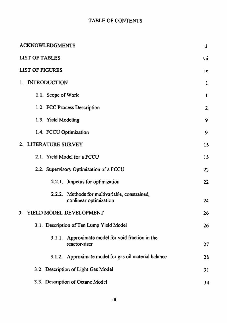
TABLE OF CONTENTS

ACKNOWLEDGMENTS ii

LIST OF TABLES vii

LIST OF FIGURES ix

1. INTRODUCTION 1

1.1. Scope of Work 1

1.2. FCC Process Description 2

1.3. Yield Modeling 9

1.4. FCCU Optimization 9

2. LITERATURE SURVEY 15

2.1. Yield Model for a FCCU 15

2.2. Supervisory Optimization of a FCCU 22

2.2.1. Impetus for optimization 22

2.2.2. Methods for multivariable, constrained,

nonlinear optimization 24

3. YIELD MODEL DEVELOPMENT 26

3.1. Description of Ten Lump Yield Model 26

3.1.1. Approximate model for void fi-action in the

reactor-riser 27

3.1.2. Approximate model for gas oil material balance 28

3.2. Description of Light Gas Model 31

3.3. Description of Octane Model 34 iii

3.4. Feed Characterization 35

4. FCCU OPTIMIZATION MODEL DEVELOPMENT 38

4.1. Process Analysis, Variable Definition, and Optimization

Criteria 38

4.2. Model Development 39

4.2.1. Approximate model for preheat fiimace 43

4.2.2. Approximate model for reactor-riser 45

4.2.3. Calculation of gas oil conversion 45

4.2.4. Approximate model for wet gas compressor

and main fiâctionator 46

4.2.5. Approximate model for the regenerator 48

4.2.6. Approximate models for estimation of carbon concentration on regenerated catalyst 50

4.2.7. Approximate models for estimation of carbon concentration on spent catalyst 51

4.2.8. Approximate model for lift and combustion air

blowers 52

4.2.9. Approximate model for catalyst inventories 56

4.2.10. Approximate model for regenerator pressure balance 57

4.2.11. Approximate model for regenerator catalyst 58 bed characteristics

4.2.12. Approximate model for the regenerator catalyst bed height 59

4.2.13. Approximate model for lift air calculations 60

4.3. Model Parameterization 61

\\

4.3.1. Description of adjustable parameter ^, 62

4.3.2. Description of adjustable parameter k^ 62

4.3.3. Parameterization often lump optimization

yield model 63

4.3.4. Description of adjustable parameter/r^2 ^^

4.3.5. Description of adjustable parameter A^^^^^ 64

4.4. Application of Optimization Technique 65

4.4.1. System constraints 65

4.4.2. Development of objective fiinction 68

4.4.3. Description of optimization routine 70

4.5. Model Sensitivity Analysis 70

5. MODEL VALIDATION 72

5.1. Yield Model Validation 72

5.1.1. Gasoline yield 73

5.1.2. Light gas yields 75

5.1.3. Coke yield 80

5.1.4. Octane value 80

5.2. FCCU Model Validation 80

5.3. Numerical Methods Validation 86

6. FCCU OPTIMIZATION 88

6.1. Description of Optimization Case Studies 88

6.1.1. Changes in product economics 88

6.1.2. Changes in gas oil feed quality 89

6.1.3. Effect of disturbances on FCCU processing 91

7. RESULTS AND DISCUSSION 94

7.1. Off-line Optimization Results 94

7.1.1. Off-line optimization results: Cases 1, 3, and 5 97

7.1.2. Off-line optimization results:

Cases 2, 4, and 6 99

7.2. Sensitivity Analysis Results 99

7.3. On-line Optimization Results 101

7.3.1. On-line optimization results: Test Case 7 103




8. CONCLUSIONS AND RECOMMENDATIONS 132

8.1. Conclusions 132

8.2. Recommendations 134

BIBLIOGRAPHY 136

APPENDICES

A. NOMENCLATURE 139

B. STEADY-STATE DATA 147

C. SUMMARY OF COMPUTER PROGRAMMING 156

VI

LIST OF TABLES

3.1 Kinetic and Thermodynamic Parameters Based on Arbel et al. (1993) 32

3.2 Gas Oil Feed Characterization 37

4.1 Process Variables used in the FCCU Optimization Model: Degrees of fi-eedom 40

4.2 Process Variables used in FCCU Optimization Model: Process Variables Determined using Newton's Method 41

4.3 Process Variables used in FCCU Optimization Model: Process Variables Determined Explicitly 42

4.4 Process Constraints used in Optimization Model 69

5.1 FCCU Optimization Validation Model: Test Run Descriptions 84

5.2 FCCU Optimization Validation Model: Sensitivity Gain Analysis 85

6.1 Product Prices for Three Modes of Operation Studied 90

6.2 Off-Line Optimization Matrix of Test Conditions 92

6.3 On-Line Optimization Matrix of Test Case Conditions 93

7.1 Summary of Off-line Optimization Results 95

7.2 Summary of Results from Sensitivity Analysis Study 100

B. 1 Steady-State Simulation Data used for the Development of Expression for Gas Oil Feed Conversion Gravity 27 147

B.2 Steady-State Simulation Data used for the Development of Expression for Gas Oil Feed Conversion Gravity 21 148

B.3 Correlation Data for Butane Based on Work by Gary and Handwerk(1984) 149

B.4 Correlation Data for Butylenes Based on Work by Gary and Handwerk(1984) 150

vii

B.5 Correlation Data for i-Butane Based on Work by Gary and Handwerk(1984) 151

B.6 Correlation Data for Propane Based on Work by Gary and Handwerk(1984) 152

B.7 Correlation Data for Propylene Based on Work by Gary and Handwerk(1984) 153

B.8 Correlation Data for Dry Gases Based on Work by Gary and Handwerk(1984) 154

B.9 Sample of Steady-State Data used for Cataslyst Inventory Correlations 155

Vlll

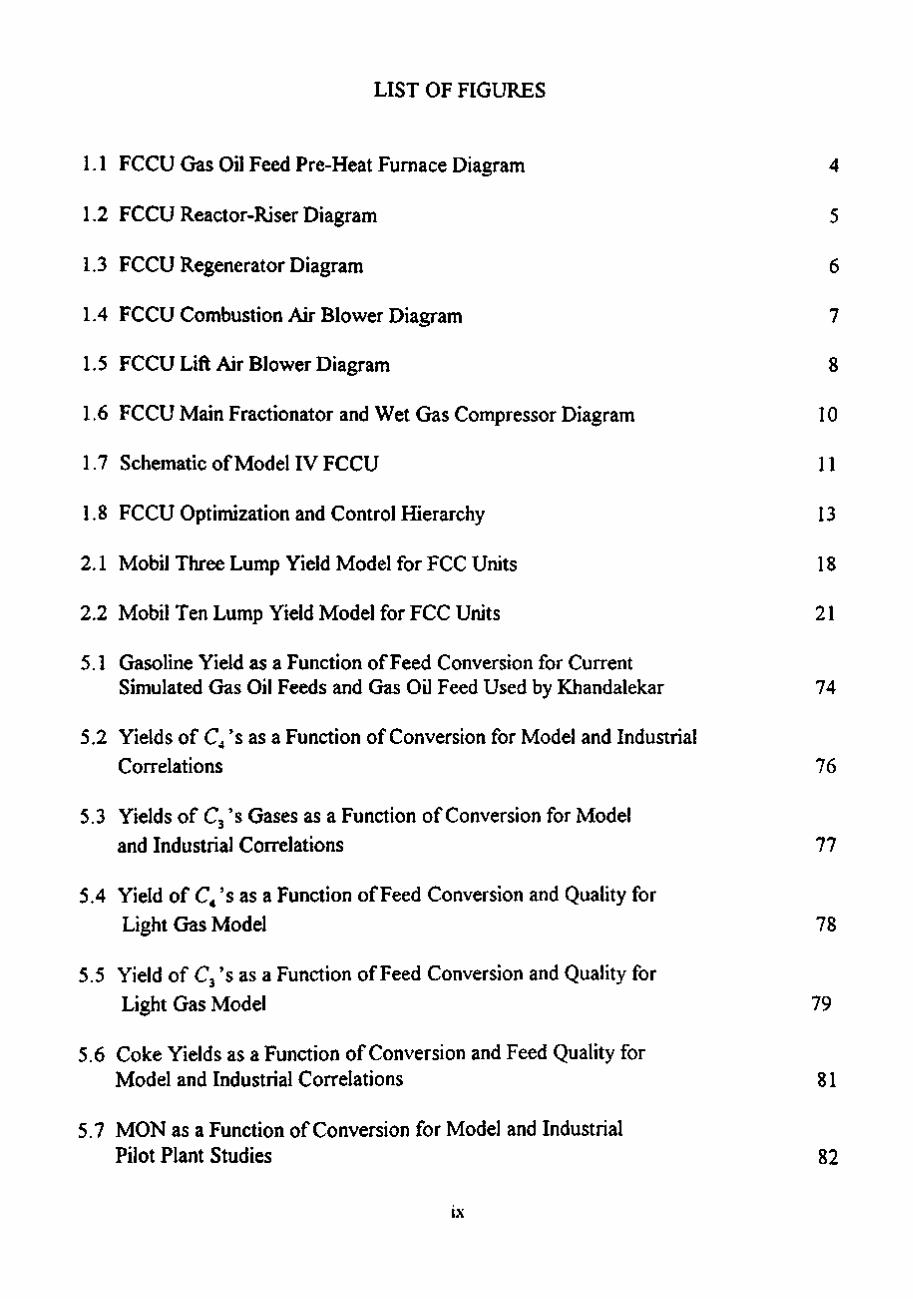
LIST OF FIGURES

1.1 FCCU Gras Oil Feed Pre-Heat Furnace Diagram 4

1.2 FCCU Reactor-Riser Diagram 5

1.3 FCCU Regenerator Diagram 6

1.4 FCCU Combustion Air Blower Diagram 7

1.5 FCCU Lift Air Blower Diagram 8

1.6 FCCU Main Fractionator and Wet Gas Compressor Diagram 10

1.7 Schematic of Model IV FCCU 11

1.8 FCCU Optimization and Control Hierarchy 13

2.1 Mobil Three Lump Yield Model for FCC Units 18

2.2 Mobil Ten Lump Yield Model for FCC Units 21

5.1 Gasoline Yield as a Function of Feed Conversion for Current Simulated Gas Oil Feeds and Gas Oil Feed Used by Khandalekar 74

5.2 Yields of Q 's as a Function of Conversion for Model and Industrial Correlations 76

5.3 Yields of C3 's Gases as a Function of Conversion for Model and Industrial Correlations 77

5.4 Yield of C4 's as a Function of Feed Conversion and Quality for

Light Gas Model 78

5.5 Yield of C3 's as a Function of Feed Conversion and Quality for

Light Gas Model 79

5.6 Coke Yields as a Function of Conversion and Feed Quality for Model and Industrial Correlations 81

5.7 MON as a Function of Conversion for Model and Industrial Pilot Plant Studies 82

ix

7.1 Regenerator Temperature for Test Case 7 104

7.2 Riser Temperature for Test Case 7 105

7.3 Gas Oil Feed Flow Rate for Test Case 7 106

7.4 Flue Gas Oxygen Concentration for Test Case 7 107

7.5 Percent Change in Objective Function for Test Case 7 108
















C. 1 Flow Diagram of Optimization Algorithm 159

CHAPTER 1

INTRODUCTION

The objective of a Fluidized Catalytic Cracking Unit (FCCU) is to convert high

molecular weight gas oils into more valuable hydrocarbon products in a safe, cost effective

manner. A few of the more valuable products include middle distillates, light olefins, and

gasoline. Since the FCCU is capable of converting large quantities of feed into more

valuable products in a matter of seconds, efficient operation of the FCCU is essential to

the economic health of a refinery. The FCC process poses a challenging control and

optimization problem since it is multivariable, nonlinear and encounters a variety of

process disturbances. In attempt to increase unit profitability, many refiners have replaced

conventional process control schemes with advanced multivariable systems. Having

reaped the economic benefits of advanced control schemes, many companies are

considering process optimization to fiirther increase FCCU profitability. Increased unit

profitability provides the impetus to develop a process optimization strategy for the FCCU

process.

1.1 Scope of Work

The primary objective of this work is to develop an on-line, supervisory optimizer for

a Model IV FCCU dynamic simulator controlled by a Process Model Based Controller

(PMBC). The purpose of the optimizer is to accept FCCU process measurements as input

and produce process variable setpoints to be used by the FCCU, which will maximize unit

profitability while honoring system constraints. The constrained optimizer will run

concurrently with the FCCU dynamic simulator.

To accomplish the primary objective a detailed yield model, which predicts the product

amounts and quality from the FCCU, will be developed. The yield model will be

implemented into the Model IV FCCU dynamic simulator developed by Khandalekar

(1993).

Operating scenarios based on the value of FCC products will be identified and used in

test cases. The effect of feed quality will be investigated by performing test runs with

feeds of different composition.

1.2 FCC Process Description

The FCC process consists of three sections:

1. Reactor,

2. Regenerator,

3. Main Fractionator.

The reactor of a FCCU consists of a feed riser line and a catalyst disengaging zone.

The riser section is a long vertical pipe which is partially contained in the reactor vessel.

After being heated to a temperature of 600-800 °F, the gas oil feed is injected into the

riser where it is mixed with hot catalyst (1200-1400 °F) from the regenerator. The

catalyst supplies the reaction sites and thermal energy required to carry out the

endothermic catalytic cracking reaction. The temperature of the product and catalyst as it

leaves the riser is approximately 900-1000°F. The residence time for the catalyst in the

riser is on the order of 2-10 seconds. The short residence time minimizes catalyst

deactivation due to coking and allows for better yields of valuable products. After the

catalyst and hydrocarbons exit the riser section the catalyst is removed from the

hydrocarbon stream in the disengaging zone of the reactor vessel. The hydrocarbon gas

stream is sent to the main fractionator for separation while the spent catalyst returns to the

regenerator where the coke produced during the cracking reaction is combusted.

Diagrams of the pre-heat fiimace, and reactor are shown in Figures 1.1-1.2.

In the regenerator, heated combustion air is mixed with the spent catalyst to burn off

the coke produced during the cracking process. Carbon dioxide, carbon monoxide, water,

and excess air are released from the regenerator as flue gas. Since the combustion of coke

from the catalyst is an exothermic reaction, the regenerated catalyst has increased thermal

energy which is required for the cracking reaction in the riser section. The temperatures

of the reactor and regenerator will remain stable if the thermal energy balance between the

two vessels is satisfied. Energy balance closure will be realized when the thermal energy

required to vaporize and crack the gas oil feed is equal to the thermal energy released

from the combustion of coke from the catalyst. The excess oxygen in the flue gas is

controlled to ensure complete and efficient combustion. Schematics of the regenerator,

lift, and combustion air blowers are shown in Figures 1.3-1.5.

The hydrocarbon products from the reactor are separated into various components in

the main fractionator. The product streams from the main fractionator include light gases

(CA and lighter), gasoline. Heavy Fuel Oil (HFO), Light Fuel Oil (LFO), cycle oil, and

fractionator bottoms. In the current study, HFO and cycle oils are lumped together as a

'T3

Gas Oil Feed

•N-

Pre—heat

Furnace

M V5

Gas Oil Feed

- ^ to Reactor

Furnace Fuel

Figure 1.1: FCCU Gas Oil Feed Pre-Heat Furnace Diagram

Regenerated Catalyst From Regenerator

To Fract ionator

Spent Catalyst to Regenerator Feed

Figure 1.2: FCCU Reactor-Riser Diagram

7. 02 Cone.

"Tcyc O ^ - - ^

Treg a

Lift Pipe

Lift Air

Cyclone

r\

M V14-

Stock Gas

Regeneroted Catalyst »• To Reactor

Combustion Air

Spent Catalyst From Reactor

Figure 1.3: FCCU Regenerator Diagram

Atmosphere

V6

0

CU) Connb. Air Blower

'F5

Vent

Ml

<s> P2 Combustion Air

to Regenerator

Figure 1.4: FCCU Combustion Air Blower Diagram

steam Vent

Atmosphere vaX

xo-Speed*/|:r

Contro '^ ' "

a

ya

\

Turbine Drive Lift Air Blower

P3

Spill Air

V9

Lift Air to Regenerator

Figure 1.5: FCCU Lift Air Blower Diagram

single product. A diagram of the main fractoantor and wet gas compressor is shown in

Figure 1.6. An overall diagram of the FCCU process is shown in Figure 1.7.

1.3. Yield Modeling

Prior to performing unit optimization a detailed product yield model must be

developed. A FCCU yield model predicts the amount of light gases, gasoline, LFO, and

HFO produced based on process conditions, feed and catalyst characteristics. Yield

models for a FCC vary in complexity from data correlations to molecular structure-based

models. Since the range of models is broad , the following criteria were used to determine

the degree of complexity required for FCC optimization purposes:

1. Model should be based on chemical engineering principles,

2. Model should be computationally efficient,

3. Model should accurately predict yields for LFO, gasoline and light gases for

different feed qualities and process conditions.

Based on these criteria, a kinetic lump model was selected to represent the yield of the

FCCU. The model is described in Chapter 3.

1.4. FCCU Optimization

The purpose of a supervisory optimizer is to generate control variable operating

targets which maximize profitability of the FCCU while honoring equipment and operating

constraints. For the purpose of this study, the supervisory optimizer is defined as a

computer program which analyzes the current operating conditions of a FCC simulation

V13

V I 2

i><l— V11 F11

•t4-T-0-

Vent

P5

Wet Gas

Main

Fract ionator

P7

f rom Reactor

t

To Vapor Recovery

Wet Gas

Comp.

Figure 1.6: FCCU Main Fractionator and Wet Gas Compressor Diagram

10

Main Fracsonator

Speed governor

Turt Q

Lift Air A Atm air Bbwer •

Atm air

Oownss'sam Separxors

Comtxjstion Air 6iow«r

Gas Oil

Spam casaVsT

Figure 1.7: Schematic of Model IV FCCU (McFarlane et al., 1987)

11

and determines what operating conditions would be required to maximize unit

profitability. The output from the optimizer are process setpoints which are given to the

PMBC constrained controller. The controller implements the optimal process setpoints

and drives the process towards the optimal conditions. Since process conditions change

over time, it is necessary to determine new optimal process setpoints periodically. Figure

1.8 shows the hierarchy of the process controller and optimizer.

The optimizer consists of an objective function, a FCCU model, and a nonlinear,

constrained, optimization problem solver.

The objective fiinction is a mathematical expression which describes the goal of the

optimization routine. For many optimization problems the objective is economic. In the

current study, the objective is to operate the process such that the slate of products

produced maximizes unit profitability.

The FCCU model consists of a series of equations which describe the FCC process.

The equations are derived from steady-state material, energy and momentum balances.

Correlations determined from steady-state process data or supplied in the literature are

also used in the optimization model development. Equations of state are used to describe

gases within the process.

To generate the optimal process setpoints described above, a computer algorithm

designed for constrained, nonlinear, optimization problems must be used. The algorithm

must be able to vary each degree of freedom while honoring all equipment and process

operating constraints, to determine the optimal values for each degree of freedom which

12

Economic and Feed Quality Informaion From Management

A

?

<

Supervisorv Optimization Aleorithm

* FCCU Optimization Model * Simplified Yield Model * SQP Optimization Algorithm * Model Parameterization

i /

Process-Model Based Constraint Controller

* Process Models * Constraint Control Models

J /

FCCU Dvnamic Simulation

* FCCU Dynamic Model * Detailed Yield Model

Q

f .

^

Figure 1.8: FCCU Optimization and Control Hierarchy

will guarantee maximum unit profitability. The Successive Quadratic Programming (SQP)

algorithm NPSOL was used in this study.

Since the equations used to model the FCC process are simplified, it is necessary to

include a feedback mechanism to adjust the model such that the model reflects the actual

process. This is accomplished by adjusting selected parameters used in the optimization

model each optimization interval. Minimizing process-model mismatch is essential to

ensure maximum unit profitability.

A typical process optimization cycle is shown below.

1. Process-model mismatch is reconciled by adjusting selected model parameters.

2. Process is at steady-state or "lined out" conditions.

3. Using pricing information supplied by management and process information from

the process, the supervisory optimizer generates optimal process setpoints.

4. Optimal setpoints are fed to the multivariable process controller.

5. Process controller drives the process to the optimal setpoint values.

In an industrial setting, the optimal process variable setpoints would be reviewed by

process operators prior to implementation. The process operator would be given the

choice of selecting or rejecting the new operating targets.

Benefits of supervisory optimization are not limited to improved unit profitability.

Ancillary benefits such as increased process knowledge in the area of constraint handling,

and the use of the optimizer off-line to study different economic and operating scenarios

are two benefits realized by companies who have installed supervisory optimizers.

14

CHAPTER 2

LITERATURE REVIEW

The focus of this work is to develop a detailed yield model for a FCCU process and a

supervisory optimization strategy to ensure maximum unit profitability. Since these two

objectives were considered consecutively, the literature review is divided as follows:

1. Yield modeling for a FCCU,

2. Supervisory optimization of a FCCU.

2.1 Yield model for a FCCU

The purpose of a yield model for a FCCU is to predict the broad range of

hydrocarbons produced during the cracking process based on process conditions, feed

quality and catalyst characteristics. The process knowledge obtained once an accurate

yield model is developed allows the optimization routine to set process conditions such

that the most valuable cracked products are produced. A successful FCCU optimization

routine requires a good yield model to work effectively.

Early attempts at modeling catalytic cracking processes only considered the

conversion of gas oil to products. Blanding (1953) developed the following expression to

predict percent volume conversion.

C kP

100.0-C WHSV (2-1)

15

where

C = percent volume conversion,

P = system pressure,

WHSV = weight -houriy space velocity, (lb oil/lb catalyst/hr),

k = cracking velocity constant.

Although it appears uncomplicated, Blanding's model requires extensive experimental data

to determine the value for the cracking velocity constant. Blanding recognized that the

cracking reaction rate was highly dependent on the catalyst fouling or coking, which varies

significantly for different feedstocks. These results are consistent with previous work

performed by Voorhies (1945).

Voorhies determined that the concentration of coke on the catalyst surface can be

represented by the following equation:

C, = ^ / ; (2-2)

where

K

m

= coking constant.

= coking constant.

t^ = contact time between catalyst and gas oil.

Jacob et al. (1976) reported that the value of constant m is approximately 0.25 and is a

function of catalyst type, while K is a function of the gas oil feed.

16

Reif et al. (1961) were among the first researchers to consider the molecular structure

of the gas oil feed when predicting product yields from a catalytic cracking process. By

measuring refractive index, specific gravity, ASTM distillation, kinematic viscosity,

percent basic nitrogen , and percent sulfijr of the gas oil feed, Reif was able to classify the

carbon types present in the molecules of the gas oil feed. These types of carbon atoms

included percentages of carbon atoms in naphthene rings, carbon atoms in paraffin chain

structures, carbon atoms in iso- and n-paraffins as side chains on naphthene rings, carbon

atoms in naphthenic rings condensed with aromatics, and carbon atoms in paraffinic chains

as aromatic rings and the associated aromatic-naphthenic structure. Reif developed

polynomial expressions which correlated these percentages of carbon types in the feed to

yields of gasoline, butane, butylene, propane, propylene, ethane and lighter gases to the

feed data. Correlations for coking, feed conversion and octane number were also

developed using the gas oil feed data. White (1969) developed similar correlations using

mass spectrometer data of the gas oil feed. Both of these modeling efforts were effective

in predicting product yields for a range of gas oil feeds but were correlative in nature.

By coupling reaction kinetics with an exponential catalyst decay function, Mobil

scientists Weekman and Nace (1970) developed a lumped species, kinetic-based model to

describe catalytic cracking. The three lump model predicts the yields of gasoline and light

gases using the reaction network shown in Figure 2.1. The differential material balances

for the gas oil and gasoline weight fractions are

^ = -0^(K,+K,)y; (2-3) at

17

Feed G C

Wt. % HFO, and Wt. % Gasoline Wt. % Coke and

1. Butylenes 2. Isobutane 3. Butane

LFO molecules

4. Propene 5. Propane 6. Gases <C2

T > 432°F Cj + < 432°F

( C, - C4, and Coke)

Figure 2.1: Mobil Three Lump Yield Model for FCC Units

18

y^ _ rh / { ^ , 1 ^ \ , . 2 /T^ t^ , .2

dt = ,{K,+K,)y]-^,K,yl (2-4)

-a.t. O. = e (2-5)

where

a. = catalyst decay velocity constant, hr"^,

O. = catalyst decay as a function of residence time,

K^ = gas oil to gasoline cracking rate constant, 1/s,

K^ = gas oil to C-lump cracking rate constant, 1/s,

K^ = gasoline to C-lump cracking rate constant, 1/s,

y^ = weight fraction of gas oil,

y^ = weight fraction of gasoline.

Nace (1974) showed that the three lump model did an excellent job predicting yields of

gasoline and light gases when virgin gas oil was used as feedstock. When increasing

amounts of previously cracked recycled material was introduced into the feed, the

model's predictive capabilities degraded. Aromatic compounds, which are prevalent in

previously cracked recycled material, needed to be taken into account when describing the

19

FCC feed. To predict yields from a broad range of feeds, the molecular structure of the

feed had to be identified more precisely.

Jacobs, Gross, and Voltz (1975) developed the ten lump model, which took into

account the molecular structure and chemistry of the gas oil feed to predict gasoline and

light gas yields, for a wide variety of feed streams. The reaction network for the ten lump

model is shown in Figure 2.2. The model incorporates the effect of nitrogen poisoning

and aromatic ring adsorption which deactivate the catalyst and reduce FCCU yields.

Arbel et al. (1995) presented an updated version of the original ten lump model which

provides a more detailed description of the reaction kinetics in the riser and regenerator.

The model allows for catalyst characterization based on laboratory data.

A drawback of the ten lump model is its inability to predict the yields of specific Hght

gas components. Plots which predict yields of light gases as a function of feed conversion

for gas oil feeds of different gravity were developed by Gary and Handwerk (1977).

Although correlative in nature, these graphs provide insight as to the effect of feed gravity

on light gas yields. Detailed reaction schemes for the production of light gases were

proposed by John and Wojciechowski (1975) and Corma et al. (1984). Both models

separated the light gas fraction into primary and secondary products. Oliveira and Biscaia

(1989) developed a model which combines components of the Mobil's ten lump model

with the light gas model proposed by Corma et al. To simplify the reaction network, the

primary and secondary gases as defined by Corma et al. (1984) are lumped as gas fractions

"Gas 1" and "Gas 2".

20

Lump Ph Nh Ash Arh PI Nl Asl Arl G C

Descrintion Wt. % Paraffinic molecules Wt. % Naphthenic molecules Wt, % Aromatic substituent molecules Wt. % Carbon atoms among aromatic rings Wt. % Paraffinic molecules Wt. % Naphthenic molecules Wt. % Aromatic substituent molecules Wt. % Carbon atoms among aromatic rings Wt. % Gasoline Wt. % Coke and

1. Butylenes 4. Propene 2. Isobutane 5. Propane 3. Butane 6. Gases < C2

Boiline range T > 648 °F T > 648 ^F T > 648 °F T > 648 °F

432 < T < 648 °F • 432 < T < 648 °F 432 < T < 648 °F 432 < T < 648°F

C5 + < 432°F

(C, - C^, and Coke)

Figure 2.2: Mobil Ten Lump Yield Model for FCC Units

21

2.2 Supervisory Optimization of a FCCU

The literature related to optimization of chemical and petroleum refining processes

can be separated into two sections.

i. Impetus for optimization,

ii. Methods for multivariable, constrained, nonlinear process optimization

2.2.1 Impetus for optimization

The driving force behind process optimization is to maximize profits from the process.

Additional benefits realized from process optimization include process knowledge and off

line design study capabilities.

Since the FCC process is complex and difficult to understand, process operators will

often run the process safely away from process constraints. This allows the process to

ride through unmeasured disturbances such as changes in ambient conditions or feedstock

quality. Lin (1993) describes this type of FCCU operation as "operating in the comfort

zone." Operating the unit in such a manner ensures process operation within specification

limits at the expense of lost economic opportunity. Maximum economic operation of a

FCCU requires the process to be pushed to the process constraints. By using a

supervisory optimizer and high speed computers, process data can be continually analyzed

and used to determine how the process should be pushed towards the operating optimum.

Dynamic Matrix Control Corporation (DMC) reported that the implementation of an

on-line optimization routine to a process will increase unit profitability by 3-5% (DMC

1992). Van Wijk and Pope (1993) of Shell Corporation reported a 10% increase in

22

process throughput and a 9% increase in gasoline production after supervisory

optimization was implemented on a Stanlow catalytic cracking unit. This increase in

production translated to a $1 MM per year profit for the catalytic cracking unit. Other

case studies of on-line optimization projects reported by Lauks, Vasbinder, Valkenburg,

and van Leeuwen (1993) include:

* a 5-10% increase in profit for a Chevron ethylene plant,

* a 1-3% increase in profit for a OMV Deutschalnd ethylene plant,

* a $3 MM/year increase in profits for a Star Enterprises crude unit.

The monetary benefits of a supervisory optimizer are well documented. Many companies

realize project payback in a matter of months (Hoffman, 1994).

An additional benefit of process optimization is the process knowledge obtained by

observing the performance of the optimized process. Information regarding constraint

handling and process bottle-neck identification can be gleaned by studying the optimal

process performance. Often the performance of the multivariable controller is enhanced

by the presence of a supervisory optimization routine. Van Wijk et al. (1993) reported

that implementation of a supervisory optimizer on a Shell corporation FCCU not only

succeeded in maximizing unit profitability but also steadied the process by handling

constraints more effectively.

23

2.2.2 Methods for multivariable, constrained, nonlinear optimization

The method used to solve an optimization problem depends on the nature of the

problem. Edgar and Himmelblau (1988) suggest that an appropriate optimization

algorithm should be chosen based on the following criteria:

1. the nature of the objective function,

2. the nature of the constraints,

3. the number of independent and dependent variables.

If the objective function and constraints are linear, optimization is usually accomplished

using linear programming techniques. Unfortunately most real worid processes are

inherently nonlinear and require special techniques to solve.

The following section reviews the different algorithms used to solve multivariable,

constrained, nonlinear process optimization problems and their characteristics. These

algorithms include Successive Linear Programming (SLP), Successive Quadratic

Programming (SQP), and Generalized Reduced Gradient (GRG) methods.

The SLP algorithm solves nonlinear optimization problems by linearizing the objective

fiinction and constraints at an individual estimate of the solution. An improved estimate of

the solution is generated by solving the linear programming problem. This cycle is

repeated until the problem converges to an optimum solution within a predetermined error

tolerance. Bodington and Randall (1979) used the SLP technique to handle nonlinearities

in Chevron's product blending program. Edgar and Himmelblau (1988) propose using

SLP techniques for large scale problems with few linear constraints. The SLP algorithm is

24

easy to implement, can handle a large number of variables and constraints, and converges

rapidly when optimum lies at the vertex of the constraints.

The SQP algorithm converts the nonlinear optimization problem into a quadratic

programming problem with linear constraints. SQP usually requires fewer iterations and

converges much faster to interior optimum points than the SLP algorithm. DMC has used

a variation of the SQP algorithm to solve numerous refinery optimization problems (DMC,

1990). The ability to handle large-scale problems efficiently makes the SQP algorithm

very powerful.

The GRG algorithm uses slack variables to convert inequality constraints into equality

constraints. The constraints are then used to reduce the dimensionality of the objective

function, thus converting the constrained problem to an unconstrained problem. Although

it can be difficult to implement, the GRG algorithm is very reliable and effective for both

vertex and nonvertex optimums (Riggs 1993). Commercially available software such as

GRG2 (Lasdon and Warren, 1986) and MINOS (Murtaugh and Sanders, 1978) has been

used successfully in refinery applications.

The software package NPSOL (Gill et al. 1986) was used to solve the FCCU

optimization problem. NPSOL uses a variation of the SQP algorithm to solve nonlinear,

constrained optimization problems. For a complete description of the NPSOL algorithm,

the reader is referred to the NPSOL User's Manual (Gill et al., 1986).

25

CHAPTER 3

YIELD MODEL DEVELOPMENT

In order to construct a supervisory optimizer for a FCCU a detailed yield model must

be used to predict the yield of hydrocarbon products based on process operating

conditions. As stated in Chapter 1, the model should be based on chemical engineering

principles, computationally efficient, and able to predict the yields of LFO, gasoline, and

light gases for different process conditions.

In this section, a description of the ten lump model, originally developed by Mobil, and

feed characterization will be offered. The light gas model, based on the work of Gary and

Handwerk (1983), will be described and implemented into the ten lump model.

3.1 Description of the Ten Lump Yield Model

The advantage of using the ten lump model (see Figure 2.2) for predicting

hydrocarbon yields from a FCCU is the ability to account for changes in kinetic rate

parameters due to feed quality changes. This model, first proposed by Jacob et al. (1974)

and Gross et al. (1976), coupled with the catalyst deactivation model developed by

Krambeck (1991), is used in this study. The model used to estimate the void fraction in

the riser is based on catalyst fluidization principles as described by Froment and Bischoff

(1990).

26

The FCC riser is modeled as a plug flow reactor with the assumptions listed below:

The model development assumes

1. Quasi steady-state conditions,

2. No slip between gas vapor and catalyst,

3. Adiabatic operations,

4. Constant temperature of gas and solid phases in the radial direction across the riser

diameter.

5. Constant physical properties,

6. No diffiisional limits.

3.1.1 Approximate model for void fraction in reactor riser

The fraction of the reactor riser which is not occupied by the catalyst is referred to as

the riser void fraction. The expressions shown below are developed by applying a force

balance from the bottom to the top of the riser. Since the Reynolds number of the catalyst

and vapor moving through the riser is greater than 1000 for a riser reactor (Froment and

Bischoff, 1991), the drag coefficient Cp remains constant at a value of 0.43.

£ = , V-^-l) (2.0)«,

^(0.3048)f;„

P.^ns

27

"^. = (0.3048)F,

fge

PcA,

u. -K4)(a^,)(g)(p,-^J

(3.0)p„C„

where

s = catalyst void fraction,

p^ - catalyst density, lb/ft ^,

Q = terminal velocity drag coefficient (C^ =0.43 if Reynolds number > 10^),

dj, - catalyst diameter, ft,

w, = superficial gas velocity, ft/s,

u - superficial catalyst velocity, ft/s.

u^ - catalyst terminal velocity, ft/s.

3.1.2 Approximate model for gas oil material balance

The material balance for the oil balance, based on the work of Jacob et al. (1976), and

Gross et al. (1976) is

f

dwt-

~dh T^r^Pc\ -\^

\

kwt. 1 +

V {\00)CORJ

f

\\ + k

1 ^ ^ -E - T - Z^-. ^^-' ^-.o exp(-d^) , (3-2)

Ah'' A-=l

^ r =

h A SO ns ns r v

F, oil

28

(.4) «i = c; ' coke »

where

(1- - ) ^ = catalyst deactivation function, (lb coke/lb catalyst) *

r^ = residence time in riser, s,

A= relative catalyst activity,

A^ = cross-sectional area of riser, ft^,

b = power in coking rate expression,

COR = catalyst to oil ratio, lb catalyst/lb oil,

E^ = activation energy of cracking catalyst of lump k, BTU/lb,

h = incremental vertical riser distance, ft,

^ris - height of riser, ft,

k^f^ = adsorption of heavy aromatics rate constant, wt^/lb catalyst,

k^Q = frequency factor for cracking reaction of lump k,

kfj = basic nitrogen adsorption coefficient, lb basic nitrogen/lb catalyst,

7 = riser temperature, °F,

wt^ = weight fraction basic nitrogen, lb basic nitrogen / lb catalyst.

Values for activation energies and frequency factors are summarized in Table 3.1.

The conversion of gas oil feed to products on a weight basis is defined as

Conv = M^tg +M't^Q. (3-3)

29

The coke material balance across the riser is based on prior work by Voorhies (1945),

Gross et al. (1976), Krambeck (1991), and Sapre and Lieb (1991).

dC ^^=r.Azb

dh vioo.oJ -E .(»-r)

K.^M-^)C,J' , (3-4)

where

y/ = feed coking tendency function,

E = activation energy for coke formation on catalyst, BTU/mole,

k^^ = frequency factor for coking rate.

The feed coking tendency term y/ is used to describe the quality of the feed. Gross et al.

(1976) describe the coking tendency function term as

y/ = 0.63 Ivv/, (0) + 0.291wt^ (0) + 0.113wt^ (0) + 2.225^/^ (0) + (3-5)

0.63 \wt^ (0) + 0.1 \wt^ (0) + \.415M>t, (0) + 0.0121wt^ (0),

where all weight fractions are evaluated before introduction into the riser.

The energy balance across the riser is based on work by Jacob et al. (1976).

dJ^

dh

F oil z F C +F C

dwt;

dh AH.

r.i ' (3-6)

at the bottom of the riser.

T. =

where

AH,, = heat of cracking reaction of lump /, BTU / Ibmole,

^H^ - heat of vaporization of gas oil feed, 150.0 BTU / lb. evp

30

Kinetic and heat of cracking parameters used in this study are based on work by Arbel et

al. (1995) and is summarized in Table 3.1.

3.2 Description of Light Gas Model

The purpose of the light gas model is to predict yields of n-butane, i-butane, butylenes,

propane, propene, and < C^ gases based on process conditions and feed quality, while

honoring the framework set by the ten lump model. Therefore,

^^x<i=^t^^+wt,^, (3-7)

where

w/,0 = weight fraction of light gases and coke produced, lb/lb feed,

^Koke - weight fraction of coke produced, lb coke/lb feed,

"M ig = weight fraction of light gas products, lb product/lb feed.

Expressions for the weight fractions of the light gases produced during the catalytic

cracking process were developed based on work by Gary and Handwerk (1984). The

expressions relate the light gas yields to volume-based conversion and feed gravity, while

honoring Equation (3-7). Using the modeling method described above, it was not

necessary to obtain highly proprietary kinetic parameter data for the formation of light

gases from the catalytic cracking of gas oil. A rigorous kinetic-based model was

attempted in this study with less than satisfactory results. The light gas model used

performed adequately when predicting product yields at different levels of conversion and

31

Table 3.1: Kinetic and Thermodynamic Parameters Based on Arbel et al.(1993).

Reactant

Lumps

HFO

HFO

HFO

LFO

LFO

Gasoline

Kinetic

Lump

Ph

Nh

Ash

Ash

Arh

Ph

Nh

Ash

Ph

Nh

Ash

Arh

PI

Nl

Asl

PI

Nl

Asl

Arl

G

Product

Lumps

LFO

Gasoline

Coke

Gasoline

Coke

Coke

Kinetic

Lump

PI

Nl

Asl

Arl

Arl

G

G

G

C

C

C

C

G

G

G

C

C

C

C

C

Activation

Energy

(Btu/mole)

16146

16146

16146

16146

16146

9920

9920

26153

15331

15331

31564

31564

9920

9920

26153

15331

15331

31564

31564

35171

Frequency

Factor

(1/s)

20.53

22.32

18.85

49.60

5.81

16.83

25.92

7837.74

15.26

28.90

27015.86

11556.90

7.30

20.24

2301.58

18.34

15.89

2867.04

788.21

19661.62

Heat of

Reaction

(Btu/lb)

25

25

25

25

25

65

65

65

225

225

225

225

40

40

40

200

200

200

200

160

32

feed quality, and was computationally efficient. A rigorous kinetic-based light gas model

would require actual FCCU process data.

Multiple regression techniques were used to develop the expressions shown below.

The data used for the regression analysis were taken from Gary and Handwerk (1984) and

are summarized in Appendix B.

For n-butane

^'^n-buune = ^ Pr,- butane

P feed

(0.037424Co«v^ - 0.06856/lP/ + 0.909615), (3-8)

for butylenes

^^butvle»e - ^ Pb utvlene

P feed

(0.1476Co«v^ - 0.06061 API - 1.69867) (3-9)

for i-butane

"^^î-buune = ^ Pi-bu tane

P feed

(O.lOlCortv^ - 0.098667^P/ - 4.20733), (3-10)

for propylene

propylene

r propylene

P feed

i^Z66EXP{0.0\956Conv;) + 016125API - 6.00875), (3-11)

for propane

propone propane

P feed

(0.360S9EXP{0.02655Conv^,)), :3-i2^

for < C, gases

wt^ =K îsi

Pfeed (0.366EXP(0.03332ConvJ- 0.3\0API + 7.13), (3-13)

where

p,. = liquid density of species i, lb/ft ^,

API = gas oil feed gravity,

K = light gas model scaling constant.

3.3 Description of Octane Model

Since the economic value of gasoline octane is driven by market forces and is very

volatile, it was highly desirable that the FCCU yield model predict an octane value for the

gasoline produced at different operating conditions. A rigorous model used to predict

octane value would require an extremely detailed molecular structure-based description of

the gas oil feed (Liguras and Allen, 1990; Quan and Jaffe, 1992) and a complete

understanding of the catalyst used for cracking. Since this type of modeling is beyond the

scope of the current work, computationally efficient expressions for the Motor Octane

Number (MON) and Research Octane Number (RON) were developed. Based on

information from the literature (Leuenberger, 1988), it was decided that the gasoline

octane number be a function of the riser temperature and conversion. The expression for

the gasoline MON is

MON = MON, +a,{T, - T,^,)+a,(Conv -COA7V,.,,^J, (3-14)

where

Conv^j^^^ = base value conversion weight fraction, 0.55,

MON = Motor Octane Number,

MON J, = base Motor Octane Number, 72.5,

RON = Research Octane Number,

7 = octane base temperature, 900 °F.

Coefficients a, and a^ were determined based on information from the literature

(Leuenberger, 1988; Hazeltine, Desai, 1993).

a, = 0.05 MON/°F,

^2 = 0.17MON/conversion.

The RON was determined using a correlation developed from literature data (Gary and

Handwerk, 1988).

RON = b,MON\b^, (3-15)

where

b^ = 1.2931 research octane/motor octane,

b^ = 12.06897 research octane.

3.4 Feed Characterization

To use the ten lump and light gas models shown above, it was necessary to describe

the gas oil feed in terms of the molecular weight, molecular species, and API gravity.

Feed characterization of FCCU feed streams is very complex and has been the subject of

current research (Liguras, 1992; Liguras et al., 1992). Using modern analytical chemistry

3D

equipment it is possible to identify thousands of different hydrocarbon species. Refiners

use many different measurements of feed properties in attempt to characterize the gas oil

feed. Since the emphasis of this work is to study FCCU optimization and control, and not

catalytic cracking chemistry, it was not necessary to develop or use a rigorous model for

feed characterization. The two gas oil feed streams considered in this study are described

in the literature (Froment and Bischoff, 1988; Nace et al., 1971). Since the mass

spectroscopy data provided in the literature were not specific with regard to the individual

weight fractions used by the ten lump model, the following assumptions were made when

determining the feed properties:

1. The molecular weights for the heavy and light lumps were 339.0 and 226.0

Ib/lbmole, respectively (Froment and Bischoff, 1988).

2. The lump weight fractions for Feed 2 were estimated using Assumption 1 above

and the mass spectroscopy data provided by Nace et al. (1971).

3. The API gravity for each feed was estimated using the calculated gas oil feed

molecular weight, boiling range, carbon-to-hydrogen ratio, and standard

correlations developed by Winn (1957).

Since feed characterization data is proprietary, the current feed characterizations could not

be benchmarked. However, for the current study, the most salient feature of the feed

characterization was that the two gas oil feeds studied were different. Table 3.2 is a

summary of the gas oil feed properties.

36

Table 3.2: Gas oil feed characterization where lumped species are given in weight fractions. The lumps are defined as shown in Figure 2.2.

Feed

API

27

21

Ph

0.17

0.17

Nh

0.20

0.25

Ash

0.24

0.26

Arh

0.12

0.26

PI

0.14

0.01

Nl

0.09

0.01

Asl

0.02

0.02

Ari

0.02

0.02

MW

310.0

332.0

API

27

21

37

CHAPTER 4

FCCU OPTIMIZATION MODEL DEVELOPMENT

Edgar and Himmelblau (1988) describe six general steps for analysis and solution of

optimization problems. A consolidation of these steps was used to develop the current

process optimization model and is summarized below:

1. Process analysis, variable definition and optimization criteria,

2. Model development,

3. Model parameterization,

4. Application of suitable optimization technique,

5. Description of sensitivity analysis.

The steps shown above were used to develop the current FCCU optimization model and

are described in the following sections.

The optimization model was used for off-line and on-line studies. Off-line studies

were accomplished using the FCCU optimization model, the optimization yield model and

the SQP optimization package NPSOL' ' (Gill et al., 1986). On-line optimization used the

optimization models described above and the FCCU dynamic simulator.

4.1 Process Analysis. Variable Definition, and Optimization Criteria

Before an accurate FCCU optimization model could be developed, it was necessary to

be well acquainted with the process. Open-loop testing and control results performed by

Khandalekar (1993) and McFariane et al. (1987) provided an excellent foundation for the

38

current study. Numerous simulation runs were performed to understand the effects of

disturbances and constraints on the process. Based on the knowledge gained from the

process study, it was determined that four independent variables, or degrees of freedom,

were required for process optimization. The regenerator temperature, riser temperature,

gas oil feed flow rate, and stack gas oxygen concentration were chosen as degrees of

freedom. It was desirable to use these variables as degrees of freedom since the previous

work on the FCCU simulator at Texas Tech University used these variables as

independent variable operating set points.

A list of the process variables which are used in the FCCU optimization model are

shown in Tables 4.1-4.3.

The remainder of this chapter is devoted to the development of the FCCU

optimization model and description of model implementation into the SQP optimization

algorithm.

4.2 Model Development

The FCCU model used for process optimization was developed using steady-state

phenomenological and empirical expressions. These expressions describe the following

subsections:

1. Firebox and preheat furnace,

2. Reactor,

3. Wet gas compressor,

4. Regenerator,

39

Table 4.1: Process variables used in the FCCU optimization model: Degrees of freedom.

Variable

T reg

Tr

F.,

0...

Variable Description

Regenerator temperature (°F)

Riser temperature (°F)

Gas oil feed flow rate (Ib/s)

% Oxygen in stack gas (mole %)

40

Table 4.2: Process variables used in the FCCU optimization model: Process variables determined using Newton's method.

Variable

F,

T,

T,

Fr,,

Fr

Px

P.


Furnace fuel flow rate (SCFM)

Gas oil feed temperature (°F)

Furnace firebox temperature (°F)

Catalyst flow rate (Ib/s)

Air flow rate to regenerator (Ib/s)

Wet gas compressor inlet pressure, (psia)

Combustion air blower suction pressure (psia)

41

Table 4.3: Process variables used in the FCCU optimization model: Process variables solved for explicitly.

Variable

p,

p.

sa

p.

p.

Crs,

c„

Ps

sucnjift

^ surgejift

L^

surge.comb

MON

RON


Reactor pressure (psia)

Regenerator pressure (psia)

Lift air turbine speed (RPM)

Lift air blower outlet pressure (psia)

Combustion air blower outlet pressure (psia)

Coke on regenerated catalyst (lb coke/lb cat.)

Coke on spent catalyst (lb coke/lb cat.)

Main fractionator pressure (psia)

Lift air inlet flow rate (SCFM)

Lift air blower surge flow (SCFM)

Catalyst level in standpipe (ft)

Combustion air surge flow (SCFM)

Motor octane number

Research octane number

42

5. Lift air blower,

6. Combustion air blower,

7. Catalyst inventories.

4.2.1 Approximate model for preheat furnace

The preheat furnace is used to heat the gas oil feed prior to entering the reactor-riser

section. The steady-state energy balance for the furnace firebox is

^ 5 =

r JTA \ ( a ^ T +

UA, KAH^J ^ \AH„J

FJ, (4-1) FU^ ^'-"-'FU-

where

(7;_7;)_(7^_7;) T =

In T -T

K.T,-TJ

a = firebox heat loss parameter, BTU/scf°F

Fj = firebox fuel flow rate, scfi s,

A H ^ = heat of combustion of firebox fuel, BTU/scf,

^LM - ôg "^^^^ temperature difference, °F,

7J = temperature of feed entering firebox, °F,

7 = temperature of firebox, °F,

UA^= firebox overall heat transfer coefficient, BTU/°F Is.

Equation (4-1) can be simplified by rewriting coefficient terms as constants a, and a^

Therefore,

43

^5=«l^ZJ^+«2^3- (4-2)

Parameters a, and AJ were calculated by Khandalekar (1993) using steady-state data

from the FCC process simulator.

The energy supplied to the gas oil feed from the firebox must ideally be the same as

the increase in sensible heat of the feed. Therefore,

F^,C^,„(T,-T,) = UAJ^, (4-3)

where

F^-i = feed flow rate, Ib/s,

^p,oii ~ h^^t capacity of gas oil feed, BTU/°F /lb,

7 = temperature of gas oil feed entering riser, °F.

Assuming constant oil heat capacity. Equation (4-3) can be rewritten as

FAT,-TO = a,T^, , (4-4)

where

UAj. ^ 3 = c

^P,oil

Parameter a^ was calculated by Khandalekar (1993) from steady-state FCC process

simulation data. Values for parameters a,, a^, and a^ are

a, = 0.02462 scC°F/s,

a 2 = l i 3 6 x l 0 - ' ° F " \

a, = 25.0 Ib/s.

44

4.2.2 Approximate model for reactor-riser

A macroscopic, steady-state energy balance was used to develop an approximate

model for the reactor-riser. The energy balance is shown in (4-5).

FrgcCp^Treg - T,) + F^„C^^,,(Tj. - T,) + F^^ConvAHcra^ = 0.0, (4-5)

where

^êrode = enthalpy ofcracking reaction, BTU/lb,

Cp^ = heat capacity of catalyst, 0.31 BTU/°F /lb,

Conv= conversion of gas oil,

F^^ = catalyst circulation rate, Ib/s,

7 = reactor temperature, °F ,

T^^g = regenerator temperature, °F.

4.2.3 Calculation of gas oil conversion

Gas oil conversion is estimated using the following expression developed by

Khandalekar (1993).

Conv = 1 =^ rr z , (4-6) (^, / ,-(^, / ,C07^)(e-='^-l)e-^^/^-) ' ^ ^

T;.^-(0.30) Jo + (0.70)r^.

Z = f C T +F C T

rgc ^ pc^reg ^ •* oil ^ poil -* 2

F C +F C rgc^pc •' oil^poil

where

45

COR = catalyst-to-oil ratio,

t^ = catalyst residence time in riser, s,

k^ = kinetic frequency factor, lb oil s/lb catalyst,

^2 = kinetic frequency factor, lb oil s/lb catalyst,

E^ = ratio of activation energy ofcracking reaction and gas constant, °F.

The parameters k^,k^, and E^ were evaluated by nonlinear regression using steady-state

FCC process simulation data. Values for /:. and E were held constant in the

optimization routine, while k^ was used as an adjustable parameter to compensate for

different feedstocks during on-line optimization. The values for k^ and E „ for all feeds

are

^2 = 6.4456, lb oil s/lb catalyst,

Ej,= 13732.96, °F.

4.2.4 Approximate models for wet gas compressor and main fractionator

The purpose of the wet gas compressor in the FCC process is to pressurize the light

gases to the operating pressure of the downstream vapor recovery unit. In this study the

main fractionator is not modeled in detail. Therefore, all gaseous products produced in

the riser are assumed to pass through the main fractionator to the wet gas compressor.

The wet gas compressor is modeled as a single-stage centrifugal compressor with a

constant speed motor. An operating curve described by McFariane et al. (1987) relates

polytropic head to volumetric suction flow.

46

The steady-state pressure balance around the compressor yields

^Vn= i ^M (4-7)

where

Fû=kuJPP(yn)4K-Pi, (4-8)

.*P(^n) = ^''''"'"''"''"^^ for V „ > 0 . 5 ,

fpp{V,,) = 0.3V,, for F„=<0.5,

Fv,, = flow through wet gas compressor suction valve, mole/s,

F,, = wet gas flow to vapor recovery unit, mole/s,

JPP(F\ 1) = nonlinear valve flow rate function, nlv(V,,),

P 5 = • reactor and fractionator pressure, psi,

P 7 = wet gas compressor suction pressure, psi,

F,j = wet gas compressor suction valve.

The performance equation for the wet gas compressor is

F^cn,^ = 11600.0 + Vl.366xlO'-0.1057^M^g' , (4-9)

Hwg = 182922.1(Crw'°''' - 1.0),

P Crw = -^,

P • ' 7

where

Crw= wet gas compressor ratio,

Hwg= wet gas compressor head, ft^ I min,

Fsucr,.wg ^ ^^^ g^s compressor inlet suction flow, ft^ I min.

47

The ideal gas law is used to obtain an expression for the gas molar flow rate through the

compressor.

520.0F P, P = IflLll J (4.10) '' (379.0)(60.0)(590.0)(14.7)

The pressure drop from the reactor to the main fractionator was estimated by McFariane

et al. (1987) as 9.5 psi. The expression relating the main fractionator pressure to the

reactor pressure is

P,=P,^t^l„„ (4-U)

where

^frac - pressure drop caused by main fractionator and piping, 9.5 psi,

P^ - reactor pressure, psi.

The wet gas compressor suction valve V,, was set to maximize throughput, subject to

preventing compressor surging. The valve value was set at 80% open.

4.2.5 Approximate model for the regenerator

Steady-state macroscopic energy and oxygen balances were used to develop

expressions to determine the regenerator temperature and excess oxygen in the flue gas.

Several assumptions were made in the development of the regenerator model.

1. The combustion of coke was modeled using the following reaction:

C + O2 -^CO^.

2. The depletion of oxygen across the regenerator bed was modeled as a plug flow

reactor.

48

3. The catalyst bed was assumed to be a well mixed CSTR; therefore, the

concentration of carbon on the catalyst was assumed constant throughout the

catalyst bed..

4. No reaction occurs in the dilute phase of the regenerator, above the catalyst bed.

These assumptions made it possible to obtain a tractable regenerator model at the expense

of process-model mismatch. Model parameterization described in Section 4.3 helped to

minimize this mismatch.

The steady-state energy balance for the regenerator is shown below.

-)Art„

(4-12)

F^C^,M - T„, ) + /vC,..„ (r„. - r„^ ) + - ^ ^ (1 - exp( J "' '"')AH,^. = 0.0

' =*»:-P(^^7S^)>

where

'B volume fraction of catalyst in regenerator,

C ^ = concentration of coke on catalyst, lb coke/lb catalyst,

F J. = total air flow rate to the regenerator, Ib/s,

k = rate expression for the depletion of oxygen, (lb coke) (s)/ft ^,

k^ = frequency factor for consumption of oxygen, (lb coke) (s)/ft ^,

O2 air = mole fraction of oxygen in air, mole oxygen/mole air,

T^.^ = temperature of air entering the regenerator, °F,

vs = superficial velocity in regenerator, ft/s,

49

^bed ^ height of catalyst bed in regenerator, ft,

AH^^ = heat of combustion of coke, BTU/lb coke.

The parameter k^^ ^^^ used as an adjustable parameter to minimize process model

mismatch

The steady-state oxygen balance for the regenerator is expressed by equating the

reduction in the number of moles of oxygen in the air with the number of moles consumed

in the coke combustion reaction.

; , FÂC,, -C^,) = F,(0.21-O, J , (4-13)

where ,

C, = conversion factor, 2.78,

O 2sg ^ oxygen concentration in flue gas, mole oxygen/mole air.

The conversion factor C, was determined assuming the composition of coke is CH and all

coke is converted to carbon dioxide. The value of C, was calculated from material

balance by Khandalekar (1993).

4.2.6 Approximate models for estimating carbon concentration on catalyst

Empirical expressions for the concentration of carbon on regenerated and spent

catalyst were developed by Cutler (1992) and Lee (1985), respectively.

An empirical expression for the concentration of carbon on regenerated catalyst as a

function of flue gas oxygen concentration and regenerator temperature was developed by

Cutler (1992).

50

^rtc = ^ rgcref (-77777; ^ \ ) e X p ( — ( - ) ) . l ^ ^^7

LM(x,y)= ^^^•^^,

In(-)

where

^reg.ref = carbon on catalyst reference, lb coke/lb catalyst,

E/R = ratio of activation energy to ideal gas constant, °F

LM = log mean function,

^2.ref - ^^^ g^s oxygen reference , moles oxygen/mole air,

T ^^gf. = regenerator temperature, K,

'^ reg,ref ^ rcgcncrator reference temperature, 944.5 K.

Steady-state reference parameters were determined using steady state simulation data and

nonlinear regression.

4.2.7 Approximate model for estimation of the concentration of carbon on spent catalyst

An empirical expression for the concentration of carbon on spent catalyst was

offered by Lee et al. (1985).

ke ^' Q . = C , , + J - , , (4-15)

C

where

k ^ = frequency factor for the formation of coke, (lb coke/lb catalyst) ^"^,

5 1

E(,f,/R = activation energy of coke formation reaction / gas constant, F°.

Parameter E^^p /R was determined using simulation data and nonlinear regression by

Khandalekar (1993). The parameter k^ was used as an adjustable parameter to minimize

process-model mismatch.

4.2.8 Approximate model for lift and combustion air blowers

Two centrifugal compressors supply air to the regenerator to combust the coke

from the spent catalyst, and to assist in spent catalyst circulation. The majority of the

regenerator air is supplied by the combustion air blower to the bottom of the regenerator

vessel. Air flow through the combustion air blower is controlled by a throttling valve on

the compressor inlet line. The lift air blower supplies air to the bottom of the lift pipe and

is controlled by manipulating a steam turbine which drives the blower.

The air flow rates from the combustion and lift air blowers were estimated using

steady-state simulation data.

F,=F,+F,, (4-16)

where

F^ = air flow rate from combustion air blower, Ib/s,

Fg = air flow rate from lift air blower, Ib/s.

Values for F^ and F^ were determined using steady-state simulation knowledge as shown

below. Given a value for Fj., the following rules were followed:

52

If Fj. is less than 58.94 Ib/s:

F, = 46.53 Ib/s,

F, =12.41 Ib/s.

If Fj. is greater than 58.94 Ib/s, and less than 66.07 Ib/s:

F^ = 46.53 Ib/s,

Fg = Fj - F^ Ib/s.

If Fj. is greater than 66.07 Ib/s:

Fg = 46.53 Ib/s,

Fy = Fj. - Fg Ib/s.

Using the ideal gas assumption and the steady-state material balance expression for

the combustion air blower, it was possible to relate the combustion air flow rate to the

combustion air suction pressure.

F . - F , =0.0, (4-17)

where

p ^ (520.0)(29.0)F,,„,,„„F,

' (379.0)(60.0)(r,,^+460.0)(14.7)-

Using (4-17) - (4-18), and the expression offered McFariane et al. (1987) (shown below in

(4-19), the combustion air blower discharge pressure was determined.

P,=i-^y+Prgb, (4-19)

where

53

F g - combustion air compressor throughput, Ib/s,

F 7 = combustion air flow to the regenerator, Ib/s,

^sucn.comb = combustlon air blower inlet suction flow, ft^,

^comb - combustion air blower discharge pipe flow resistance factor,

Xh/sl^psia ,

P , = combustion air blower suction pressure, psi, f . t

P 2 = combustion air blower discharge pressure, psi, ^ <(-

F fc = pressure at bottom of the regenerator, psi,

7 , = atmospheric temperature, °F.

A head capacity equation relating suction volume to discharge pressure was

provided by McFariane et al. (1987).

F^^,con^ = 45000.0 4- Vl.581xlO^-1.249xlO^F,^,^ (4-20)

^ .a ,e=14.7^ (4-21) -* 1

where

P base ~ combustion air blower base suction pressure, psi.

The lift air compressor was modeled as a single-stage centrifugal compressor

driven by a variable speed steam turbine with a speed control governor. Assuming steady-

state conditions, the air flow into and exiting the lift air blower is the same.

F,-Fg= 0.0

54

The steam turbine is controlled by manipulating the steam valve, V,,^ . The expression for

the lift air motor speed is

sa = sa^^^+V,^ (WOO). (4-22)

A linear expression for the steam valve position as a fiinction of the lift air flow rate was

determined from steady-state simulation data.

Vi-fl = (0.\2626)F, - 1.467172 , (4-23)

Using the ideal gas assumption, an expression for the lift air blower inlet suction flow rate

was developed.

P ^ (14.7)(379.0)(60.0)(r„,+460.0)

""•"" (520.0)(29.0)(P„„)(F,)

The lift air blower surge flow is expressed as a function of the discharge pressure.

^» ..„;« =5025+112. P3, (4-25)

where

F3 = lift air blower outlet pressure, psi.

The outlet pressure from the lift air blower is given as a function the lift air flow rate and

pressure at the bottom of the lift pipe.

Py = C-^ ) ' + n „ (4-26)

where

k,,^ = lift air blower discharge flow resistance factor, 5 Ib/syjpsi,

55

^bip - pressure at the bottom of the lift pipe, psi.

4.2.9 Approximate model for catalyst inventory in the regenerator, stand pipe, and reactor

Empirical expressions for the catalyst inventories in the regenerator, stand pipe and

reactor were developed using steady-state simulation data as a function of the total air

flow rate and regenerated catalyst flow rate. Using multiple linear regression and

simulation data shown in Appendix B, the expression for catalyst inventories in the

regenerator, stand pipe and reactor are

Wr„=h,+b,,F,+b„F^,, (4-27)

W^=h,+h,F,+b,,F^,, (4-28)

where

by = correlation coefficients,

W^ = weight of catalyst in reactor vessel, lb,

W^^g = weight of catalyst in regenerator, lb,

W = weight of catalyst in stand pipe, lb. sp

The values for the correlation coefficients used in equations (4-27) to (4-29). For the

catalyst inventory in the regenerator:

b,, =361613.4 lb,

56

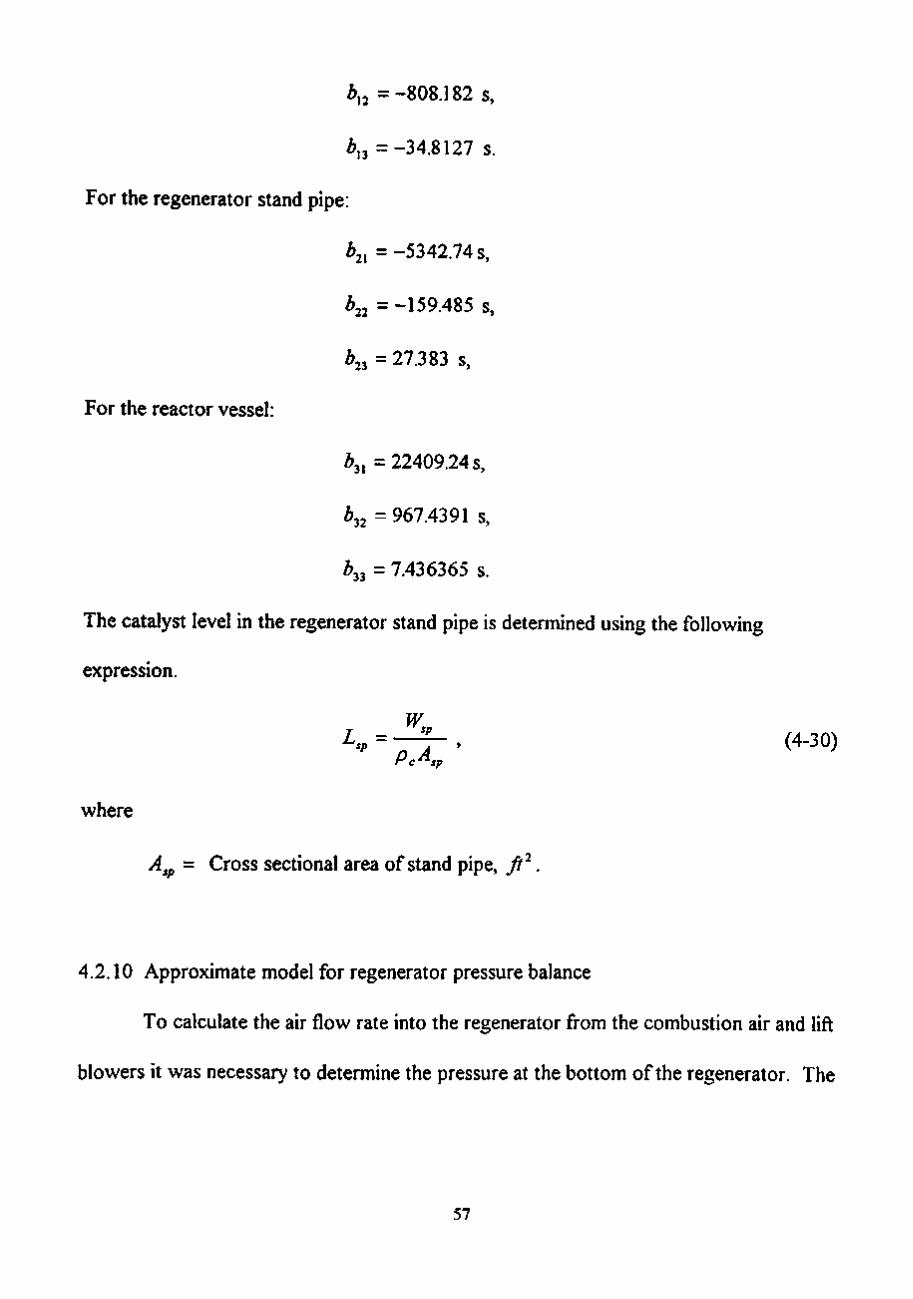
Z>,2 =-808.182 s,

b,^ =-34.8127 s.

For the regenerator stand pipe:

>2, =-5342.74 s,

Z>22 =-159.485 s,

>23 =27.383 s.

For the reactor vessel:

Z>3, = 22409.24 s,

Z>32 = 967.4391 s,

33 = 7.436365 s.

The catalyst level in the regenerator stand pipe is determined using the following

expression.

Lsp=—^. (4-30)

where

A^p = Cross sectional area of stand pipe, ft^.

4.2.10 Approximate model for regenerator pressure balance

To calculate the air flow rate into the regenerator from the combustion air and lift

blowers it was necessary to determine the pressure at the bottom of the regenerator. The

57

pressure was determined by performing a force balance across the regenerator catalyst

bed.

W Pr.b=P6+ , (4-31)

^ ' ' (144)(4.,)

Based on steady-state simulation data, a constant regenerator pressure was assumed in

the optimization model.

4.2.11 Approximate model for regenerator catalyst bed characteristics

The regenerator catalyst bed height and superficial gas velocity through the catalyst

bed were required to determine pressure terms in the lift pipe. Empirical expressions for

the superficial gas velocity, density of the catalyst in the dilute phase through the

regenerator catalyst bed and volume fraction of catalyst in the regenerator bed were

developed by McFariane et al. (1987).

y. = FA—^), (4-32) 8 reg

(520)(F,) P. = (379)(14.7)(7;,^+460)

(4-33)

1.904 + 0.363V5 - 0.048V5-,, , . _ .. e^ = min(l, max(f ^, Sj- + • )), (4-34)

2i . 'bed

P B =^-ê>

where

£^ = effective void fraction in regenerator dense phase bed,

58

Pg = density of gas in the regenerator, lb I ft^

The density of the catalyst in the dilute phase of the regenerator is a fiinction of the

superficial gas velocity through the regenerator.

/ ?= -0 .878+ 0.582v^ , (4-35)

where

p^ = density of catalyst in the dilute phase, lb I ft^.

4.2.12 Model for the regenerator catalyst bed height

An empirical model for the catalyst bed height in the regenerator was offered by

McFariane et al. (1987).

^bed = m i n ^ z_,(2.85 + 0.8v,+ '^reg P cdil-^reg"^ c\ reg eye

eye ^re.P reg H c,dense

w

Pc. dil 1-V r .dense y

(4-36)

Pcdense " Ppart (^ ^ / ) '

£, =0.332+0.06V, , • /

where

Sj. = apparent void fraction in the regenerator dense phase bed.

Pc dense = denslty of catalyst in the dense bed, lb I ft^,

part density of settled catalyst, lb I ft^,

z^ - height of cyclone inlet, 45 ft.

59

4.2.13 Approximate model for air lift calculations

Air from the lift air blower is used to assist the circulation of catalyst. By increasing

the flow rate of lift air, the density of the catalyst in the lift pipe decreases. This lowers

the head pressure and increases the catalyst through the spent catalyst return line.

The steady-state representation for the density of catalyst in the lift pipe is

rgc

^cat,lift'Îp + Pair.. - Pun = 0 0 , (4-37)

(29)F, otr.g F(r,,+460) '

F„ V air.lift

'ÎpPair.i

^catMft = max^ F

âir,lift ^slip ' rgc

ÎpP port

where

p^.^ = density of air at regenerator conditions, lb I ft^,

\ = cross-sectional area of lift pipe, ft..

sc temperature of spent catalyst entering the regenerator, °F,

V = velocity of air in lift pipe, ft/s. air.lift

cot,lift = velocity of catalyst in the lift pipe, fi^s.

^slip = slip velocity between air and catalyst, 2.2 ft/s.

60

The pressure at the bottom of the lift pipe is expressed as the sum of the regenerator

pressure, lift pipe head pressure, and weight of catalyst in the lift pipe. Therefore,

144.0 144

where

/7,, = height of lift pipe, 34 ft,

2,p = height of lift pipe discharge, 11 ft.

4.3 Model Parameterization

Benefits of FCCU optimization can only be realized if the FCCU optimization model

accurately describes the FCCU process. To minimize this process-model mismatch,

adjustable parameters, which are common to the process and optimization model and

whose exact values were not precisely known, were selected. Process-model mismatch

was minimized using the following parameters:

1. The frequency factor for the formation of gasoline (A:,) from (4-6),

2. The frequency factor for the formation of coke (kj from (4-1T),

3. The frequency factors for the cracking of gas oil from (3-2),

4. The frequency factor for the depletion of ox7gen (k^^) from (4-12),

5. The enthalpy of gas oil cracking, AH^^^^ .

Complete explanations for the development of the model parameters are shown below.

61

4.3.1 Description of adjustable parameter k^

The frequency factor for the formation of gasoline from gas oil (/:,) was used as an

adjustable parameter to ensure that the gas oil conversion predicted by the model

accurately predicted the gas oil feed conversion observed in the FCCU simulation. As

described in Section 4.2.3, steady-state simulation yield data were used to evaluate

parameters k^ and Ej, off-line. These parameters were valid for both feeds investigated.

The adjustable parameter /:, was used to compensate for the feed quality which was being

processed. Equation (4-6) was used to determine /:, on-line using simulation data. An

average parameter value was obtained by filtering the parameter value between

optimization cycles.

4.3.2 Description of adjustable parameter k^

Since it was not possible to measure the concentration of carbon on the regenerated

and spent catalyst, expressions developed by Cutler et al. (1992), and Lee (1985),

respectively. Equation (4-14) was used to estimate the carbon concentration on the

regeneration. By substituting the expression for the steady-state oxygen balance (4-13)

into the correlation used to predict the concentration of carbon on spent catalyst (4-15), it

was possible to determine the value of parameter k^ in terms of measurable process

variables. This expression is shown in equation (4-39).

62

r

k =

^F,(0.2\-O,,l\00.)^"^

\

2sg

C F ^\-^rgc J

^-^Vi^rjTregk) \

\LM{01\,O2^l\00))

0.4 \

V

/ cfr )

K,

J

(4-39)

where

K = Q^^ZA/(0.21,O,^,.^)exp(£77;.^,).

The parameter k^ was adjusted on-line to compensate for the coking characteristic of the

gas oil feed being processed. The parameter value was filtered prior to being used in the

optimization routine.

4.3.3 Parameterization of the ten lump optimization yield model

Process-model mismatch between the simulation product yields and the optimization

yield model was minimized by adjusting the frequency factors in the optimization yield

model. In order to reduce the dimensionality of the parameterization problem, the FCCU

products were group as HFO, LFO, gasoline and light gases. Six parameters were used to

adjust the frequency factors such that the yields predicted by the optimization yield model

were consistent with the simulation data. The frequency factors were multiplied by the

adjustable parameters. Filtered simulation yield data were used as parameterization

targets. The SQP optimization algorithm NPSOL™ (Gill et al., 1986) was used to

determine the adjusted frequency factors. The objective of the frequency factor

optimization problem was

Objfff ={AHFOy +(ALFOy +iAM't{9))- +(Aw?(10))\ (4-39)

63

mod '

where

AHFO= HFO,^-HFO^^,

ALFO= LFO „-LFO

Awt(9)= M>t{9),„-M>t{9)^^,

Awt(10)= M'K10)^^-M'/(10)„^,

where subscripts

sim= process simulation value,

mod= optimization yield model value.

The product of the yield model frequency factors and the six parameters were used to

adjust the ten lump optimization yield model frequency factors. This parameterization was

effected prior to each optimization cycle.

4.3.4 Development of adjustable parameter k^-^

The frequency factor for the depletion of oxygen in the coke combustion reaction in

the regenerator was used as an adjustable parameter to minimize process-model mismatch

in the macroscopic energy balance expression (4-12). The value of this parameter was

determined on-line. The parameter was filtered between optimization cycles.

4.3.5 Development of adjustable parameter AH^^^^

A macroscopic energy balance for the reactor riser was shown in expression (4-5).

The enthalpy of gas oil cracking, tJI^^^, was used as an adjustable parameter to

64

compensate for the quality of the gas oil feed. The parameter was evaluated on-line using

expression (4-5), and filtered between optimization cycles.

4.4 Application of Suitable Optimization Technique

The previous sections describe the steady state optimization model, and optimization

yield model for the FCCU. The current section describes how the SQP optimization

software package NPSOL^"^ (Gill et al., 1986) is used in conjunction with the process

models and FCCU system constraints. This section describes the FCCU constraints,

development of economic objective function, and a description of the optimization

solution method.

4.4.1 System constraints

System constraints encountered in the FCC process are classified as equipment and

operational constraints. Equipment constraints represent physical limitations which eflfect

FCC operation. Operational constraints are desired operating limits based on

environmental, safety or economic conditions. The following section lists the equipment

and operational constraints considered in this study.

The equipment constraints were divided into four areas:

1. Flows,

2. Compressor or blower limits,

3. Pressures,

4. Temperatures.

65

Maximum flow rates for the gas oil feed and preheat furnace fuel flow are considered

in this study. These constraints are

gas oil feed rate < 132.0 Ib/s,

fuel flow rate to preheat furnace < 39.5 Ib/s.

Constraints for the wet gas compressor, combustion and lift air blowers were

considered in this study. For the wet gas compressor and the blowers, the suction valves

must be between 0 to 100% open. For the lift air blower this corresponds to a blower

speed of

5000 < 5a < 6100 rpm.

Metallurgical pressure limits on the regenerator, fractionator, and reactor are given as

F, <39.7 psig,

P, < 39.7 psig,

P^ < 30.2 psig.

Metallurgical temperature limits for the regenerator, reactor riser, and firebox are

7;,^<1350°F,

T;, < 995 °F,

T; <I7OO °F,

respectively.

The operational constraints considered in this study were categorized into four groups:

1. Blower surge constraints.

66

2. Total combustion constraints,

3. Reactor / Regenerator pressure difference,

4. Regenerator stand pipe level constraint.

The surge point for the lift air blower is given as a fiinction of the discharge pressure.

^^^...y.= 5025.0+ (112.0)F3.

The lift air blower surge constraint is expressed as

P '^ P ^sucn.lift -^ ^surge,lift •

The surge point for the combustion air blower was defined as

^„ ..™»» =45100 SCFM.

The combustion air blower constraint was

F < F sucn,lift surge,hft '

To ensure total combustion of coke in the regenerator, the following constraints to the

flue gas oxygen concentration and regenerator temperature were used.

r,,^> 1265.0 °F,

02sg > 0.50%.

Since the driving force for catalyst flow is the pressure difference between the

regenerator and reactor, an operational constraint was applied to the pressure difference to

ensure catalyst flow. Therefore,

-5.0 < AF^ < 2.0 psi,

AF^ =Pe-P, psi.

67

An operational constraint was placed on the catalyst level in the regenerator stand pipe

to ensure catalyst flow to the reactor.

0.0 < F„ < 20.0 ft. sp

A summary of the process constraints is shown in Table 4.4.

4.4.2 Development of objective function

The objective function used in the optimization routine is expressed as

18

F{x)= Z(-PMO + P^f„-Pf...)iF^,), (4-39) 1=1,1*10-12

/ ^ = 2 ^ ^ ^ ± M ^ - 8 5 . 6 9 (4-40)

where

/ = octane value function, octane value, • / OV ' '

p. = value of lumped species i, $/lb,

p = value of gasoline octane value, $/lb/octane value,

wt(i) = weight fraction of species I.

The values for p. are based on the economic climate and are varied in this study. The

different pricing structures considered in this study are described in Chapter 6.

68

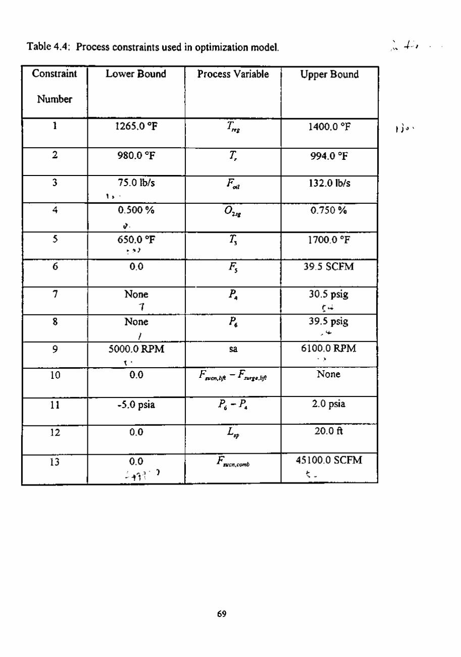
Table 4.4: Process constraints used in optimization model. .1 -/-

Constraint

Number

1

2

4

5

6

7

8

9

10

11

12

13

Lower Bound

1265.0 °F

980.0 °F

75.0 Ib/s y >

0.500 %

650.0 °F

0.0

None 1

None

/

5000.0 RPM

0.0

-5.0 psia

0.0

0.0

Process Variable

T reg

I

F..,

O^n

T,

F,

P,

P.

sa

F - F sucn,lift surge,lift

P,-P,

4,

P svcn.comb

Upper Bound

1400.0 °F

994.0 °F

132.0 Ib/s

0.750 %

1700.0 °F

39.5 SCFM

30.5 psig

39.5 psig

6100.0 RPM > >

None

2.0 psia

20.0 ft

45100.0 SCFM

ij'

69

4.4.3 Description of optimization routine

FCC optimization was affected using FCC subsection models developed in the

previous sections and the optimization variables. The decision variables 7 ^ , 7 , F^,,, and

02sg were set by the optimization software NPSOL''"' (Gill et al., 1986) each optimization

iteration until optimal values were obtained. Seven dependent process variables were

solved simultaneously using FCC subsection models and Newton's method. The

remainder process variables were determined explicitly. A summary of FCCU process

variables is shown in Tables 4.2-4.4. Appendix C provides a flow diagram of the FCCU

optimization algorithm.

4.5 Description of Sensitivitv Analysis

A sensitivity analysis was performed to determine the effect of parameter uncertainty

on the optimization routine. Since the model parameters previously discussed are used to

reconcile process-model mismatch and are adjusted on-line, these parameters have an

inherent uncertainty which may affect the optimal solution. Perturbations were introduced

to each of the parameters to study this effect. The following section describes the

sensitivity analysis used in this study.

The sensitivity analysis was performed off-line using the optimization model and the

SQP optimization software package NPSOL^M (Gill et al., 1986). An optimal base case

was defined to use as a benchmark. Increases and decreases in AH^^^^ , AH^^^„ /:,, and

k^ were introduced in separate off-line optimization runs and objective fijnction values

were compared to the optimal base case. By performing this study, it was possible to

70

estimate the effect of process-model mismatch on FCCU process optimization. The

results of this study are shown in Table 7.2 and are discussed in Chapter 7.

71

CHAPTER 5

MODEL VALIDATION

In any modeling exercise it is necessary to compare the model resuUs with process

data to ensure that the model describes the actual process. In absence of process data, the

developed model can be compared to other accepted models, correlations, or literature

values. This section is devoted to comparing the yield and FCCU optimization models to

actual FCCU data. Since FCCU process data is highly proprietary, the current yield

model will be compared to data obtained from the literature and other benchmarked

models. Yield profiles for the two feeds investigated are provided to demonstrate the

effect of feed quality on product yields. The FCCU optimization model will be compared

to steady state data generated by the dynamic FCCU simulation (Khandalekar, 1993).

Finally, the accuracy of the numerical methods used in this study are discussed to

demonstrate numerical method validation.

5.1 Yield Model Validation

The FCCU model consists of the ten lump and light gas models. In the absence of

actual process data, several different sources were used to verify the yield model. There

are inherent disadvantages to using this method for FCCU yield model validation. For

instance, there are different types of FCC units in operation. Units use different catalyst

types and processing equipment which give each FCCU its own yield characteristics. This

will lead to unit-to-unit variability. This phenomenon is most pronounced in the formation

72

of ethane, methane and hydrogen. Since these species are only formed by thermal

cracking, and each FCCU has different thermal cracking characteristics, wide ranges of

these species should be expected when analyzing data from many different units.

The results from yield model simulation runs were compared to literature data and

other yield models. Simulation yields of gasoline, C3 's, C^ 's, coke, and octane are

compared to literature values on the following pages. In the absence of Model IV FCCU

process data, general trends, rather than absolute yield values will be noted.

5.1.1 Gasoline yield

The ten lump model developed by Mobil has shown good correlation with

experimental and industrial data (Jacob et al., 1976). For the purpose of the current model

verification, the gasoline yields produced by the current ten lump model for two different

feeds were compared to the gasoline yield produced using a three lump model developed

by Lee (1987) and used by Khandalekar (1993). The three yield profiles shown in Figure

5.1 show the effect of feed conversion on gasoline yield. Since the catalyst type and feed

quality are critical variables in the determination of gasoline yield, an absolute comparison

often lump model yields to the Lee model yield is not recommended. However, it is

apparent that the current model has the same general characteristics as the model

developed by Lee (1987).

73

50 55 60 65 70 Conversion (wt%)

75 80 85

— API = 27 (Model) API = 21 (Model) - ^ Khandalekar (1993)

Figure 5.1: Gasoline Yield as a Function of Feed Conversion for Current Simulated Gas Oil Feeds and Gas Oil Feed used by Khandalekar (1993).

74

5.1.2 Light gas yields

Results from the current light gas yield model were compared to industrial data from

several FCC units which were provided in the literature. Figure 5.2 compares the current

C4 model to four different correlation's found in the literature. It is important to note the

disparity between each of the models. This difference between the models was expected

since light gas yields are functions of process properties which were not specified.

Catalyst type is an example of such a property. Based on this premise, the current model

provides a good representation of C4 yields as a function gas oil conversion.

Figure 5.3 compares the current model for the prediction of C3 gases as a fiinction of

gas oil feed conversion to an industrial correlation developed by Maples (1993). A

comparison of the correlations shows that the current model has a greater slope than the

industrial correlation. Because of the reasons stated above, differences in the current

model and the industrial correlation were expected. By plotting individual data points

which Maples (1993) used to develop the industrial correlation, it is evident that the

current model lies well within the scatter of the industrial data. Therefore, the current

model provides a reasonable representation of C3 gases yield as a fiinction of gas oil

conversion.

Figures 5.4-5.5 show the yields of each light gas species as a function of gas oil

conversion as predicted by the light gas model for two different feed qualities. These yield

profiles are instructive in illustrating the effect of feed quality on the individual light gas

species predicted by the model.

75

25

^^20

o en

0) > •

315

10

60 65 70 75 Conversion (vol.%)

80

— Current Model H Nelson, 1973 © Wachteletal., 1972 A Maples. 1993

Voorhies et al. 1964

Figure 5.2: Yields of C, Gases as a Function of Conversion for Model and Industrial

Correlations.

76

65 70 75 Conversion (vol.%)

80 85

Current Model — Maples, 1993 Sample of Data used by Maples, 1993

Figure 5.3: Yields of C^ Gases as a Function of Conversion for Model and Industrial

Correlations (Maples, 1993).

77

12

10 -

_ 8

o >

>-4 -r-

2 -

70 75 80 85 90 Conversion (vor/o)

I

^ ^

1— ~» •

o

_... •

1

1 r

V

-

o

n

V •

--o~-

—

n

1 1

V

o

—

•

V

® o

n

' 1 1 '

V — • - — •••

o

— —

•

1

V •

^ k

o

-

D •1

I (

•

«

•

V

- • Q -

n

• <

i 1

95 100

-»-nC4 - API=27 • nC4-API=21 • =C4 - API=27 V =C4-API=21 ® iC4-API=27 o iC4-API=21

Figure 5.4: Yield of C, 's as a Function of Feed Conversion and Quality for Light Gas

Model.

78

O

o

0 -

•

!

V

i h -

•

\—

V

— i

T V

- i '• \ - ^ \ i

70 75 80 85 90 Conversion (vol%)

95 100

=C3-API=27 n =C3-API=21 • nC3 - API=27 v nC3-API=21

Figure 5.5: Yields of C, 's as a Function of Feed Conversion and Quality for Light Gas

Model.

79

5.1.3 Coke yield

To verify the expression for coke yield shown in Equation (3-4), an industrial

correlation (Handwerk, 1984) and raw data (Maples, 1993) were compiled and compared

in Figure 5.6. The comparison shows that the model used in the current study displays the

same characteristics as the industrial data and predicts a coke yield profile which falls

within the scatter of the industrial data.

5.1.4 Octane value

The correlation developed to predict the MON value as a function of conversion and

riser temperature was compared to industrial data provided by Desai and Haseltine (1989)

and is shown in Figure 5.7. The current correlation was developed from information

found in the literature (Desai and Haseltine, 1989) and qualitatively validated by industrial

experts (Hofifrnan, 1994; Albus, 1994). Since octane value is strongly dependent on

catalyst activity and structure, and is proprietary, an absolute validation of the model

results to industrial data is difficult. However, the comparison is instructive in showing

that the model predicts the same trends that are seen in industrial FCC units and is

performs adequately for optimization purposes.

5.2 FCCU Optimization Model Validation

The FCCU optimization model was validated by performing a steady-state gain

analysis. This analysis compared the process gains generated by the process simulation to

80

0.1

0.08 --

^ 0.06 f i 0)

Q 0.04 ^

0.02 --

60 65 70 75 Conversion (vol.%)

80 85

API = 27 (Model) ^ API = 27 (Handwerk, 1984) Raw Data from Maples (1993)

Figure 5.6: Coke Yield as a Function of Conversion and reed Quality for Model and Industrial Correlations (Maples, 1993).

81

85

83

81

O

79 --

77 --

75

60 65 70 75 Conversion (wt.%)

80

Model Desai, Haseltine (1989)

Figure 5.7: MON as a Function of Conversion for Model and Industrial Pilot Plant Studies (Desai and Haseltine, 1989).

82

the process gains predicted by the FCCU optimization model. The analysis was

performed using the following method:

1. Perform four simulation runs using the controlled variable setpoints summarized in

Table 5.1. Record manipulated variable values.

2. Using the same controlled variable setpoints, obtain manipulated variable values

predicted by the FCCU optimization model. Record these values.

3. Determine the process gains for the steady-state simulation and FCCU optimization

model using Run 1 as the reference case.

4. Compare the gains as shown in Table 5.2.

The gain information shown in Table 5.2 is an indication of how well the FCCU

optimization model captured the steady-state characteristics observed in the actual process

simulation. As the cases with most steady-state gain analysis, the most important gains

are the diagonal elements. Each diagonal element considered the controlled variable, and

the manipulated variable which was adjusted to maintain the controlled variable setpoint.

These are the critical elements of Table 5.2

Table 5.2 shows that for the runs where the riser and regenerator temperature were

varied from the reference conditions, the signs of the gain were identical. The values of

the gains show better agreement for changes in the riser temperature than for changes in

the regenerator temperature, or flue gas oxygen concentration. For cases where the flue

gas oxygen concentration was changed from the reference conditions, the sign of the gains

did not agree in two of three elements. For the diagonal element there was sign

agreement. What is not indicated in Table 5.2 is that for changes in the flue gas oxygen

83

Table 5.1: FCCU Optimization Model Validation: Test Run Descriptions Feed API=27.

Run

Base

AT,

^Tr^

Ô^s,

Fo, Ib/s

115.0

115.0

115.0

115.0

T; °F

990.0

994.0

990.0

990.0

T °F reg

1264.29

1264.58

1261.87

1263.41

Trde-Air

0.780

0.7180

0.825

0.979

84

Table 5.2: FCCU Optimization Model Validation: Sensitivity Gain Analysis Feed API=27.

Ar, Simul.

AT^ Model

AT;^ Simul.

AT Model

AO^jg Simul.

AO^^ Model

APF

AF3

-0.510 ' ft'Is

-0.973 ' //'A

0.632 ^ ft'ls

1.621 ° ^

-0 055 ^^^ °/

+0.176 '"^^ °/ ft'ls

APV

rgc

0.0641 ° ^ Ib/s

0.0838 ° ^

-0.192 ^

-0.073 ^

0.008 '" ^ "'"

-0.035 '" ^ "/°

APV

AFj,

0 rr

0.871 ^

0.661 ^ 0 TT-

-1.001 ^

-1.194 ^

0 067 ^ ""''

Ib/s

85

concentration, insignificant changes in the catalyst flowrate and fiimace fijel flowrate were

observed. This tended to exaggerate the gain results for the off-diagonal elements.

The steady-state gain analysis was used to identify process-model mismatch, especially

in the regenerator modeling.

5.3 Numerical Methods Validation

The ten lump yield and steady state optimization models implemented in this study

used LSODE (Hindmarsh, 1985) to evaluate stiff differential equations, Newton's method

for the solution of a system of nonlinear equations, and NPSOL™ (Gill et al., 1986). The

integrity of the numerical methods used to model the original dynamic simulator were

validated by Khandalekar (1993).

Since the differential expressions used in the ten lump model were stiff, the software

package LSODE (Hindmarsh, 1985) was used to integrate the differential equations.

Significant improvements in model accuracy and computation time were realized by using

LSODE instead of the Runga-Kutta routine. The Runga-Kutta routine required a

maximum step size of 0.015 ft to integrate across the riser to achieve consistent solutions

for the product yields. Yield model integration using LSODE was approximately ten

times faster than yield model integration using the Runga-Kutta routine. An absolute error

tolerance of 1.0 x 10"^, and a relative error tolerance of 1.0 x 10" were required for

integration accuracy. For a complete description of the LSODE integration routine, the

reader is referred to the software documentation (Hindmarsh, 1985).

86

Newton's method was used to solve six nonlinear equations which described the

optimization model along with other process variables which are solved for explicitly. A

relative error of 1.0 x 10"^ was used to guarantee an accurate model solution. Since the

most current process variable values were used as initial guesses for Newton's method, a

tractable solution was found for each set of degree of freedom variables.

The SQP software package NPSOL™ (Gill et al., 1986) requires the user to provide a

driver program, which includes the system constraints, an objective fijnction, and an input

file. The input file contains several parameters which specify problem solution accuracy

and solution method. A description of the input parameter is provided in the NPSOL*™

software documentation (Gill et al., 1986).

Because of the computer memory limitations imposed by the MS-DOS operating

system, the simulation study was performed on a UNIX-based, 90 MHz Pentium personal

computer. The ratio of CPU-to-real time was approximately 0.70:1.00 for the process

simulation. For the majority of the on-line optimization cycles, optimal process setpoints

were determined in less than two minutes.

87

CHAPTER 6

FCCU OPTIMIZATION

As stated in the previous chapters, a successful FCCU optimization routine requires a

detailed yield model, an optimization model which accurately describes the FCCU

process, a method to parameterize the FCCU optimization model in order to minimize

process model mismatch, and a nonlinear, constrained optimization routine. Having

developed and implemented the items listed above, Chapter 6 is devoted to describing the

off-line and on-line test cases investigated in this study.

6.1 Description of Optimization Case Studies

The optimization scenarios investigated in this study were classified into the

following three areas:

1. Changes in product economics (off-line optimization),

2. Changes in gas oil feed quality (off-line optimization),

3. Effect of disturbances on the FCCU (on-line optimization).

The test cases considered in this study fall into one of the areas listed above and are

described in the following sections.

6.1.1 Changes in product economics

The value of FCCU products experience both predictably and unpredictable changes.

The most important predictable changes m product values are due to seasonal product

88

demand. During the summer months, the value of gasoline is at a premium. During the

winter months, LFO becomes more valuable since it is used as home heating fuel.

Unpredictable product value changes are very difficult to identify a priori. World politics

affecting crude oil prices, scarcity of light gas products used in the plastics industry, and

the unpredictable value of octane are examples of the changing economics of FCCU

products. Seasonal changes in product values were considered in Modes 1 and 2. Mode

3 considers the scenario where the light gas products are at a premium. Product prices

were taken from the literature (Desai et al., 1992) and private discussions with industrial

experts (Hoffinan, 1995). These modes are summarized below.

Mode 1: Gasoline Mode. Also referred to as medium severity or Summer mode.

Mode 2: LFO Mode. Also referred to as low severity or Winter mode.

Mode 3: Light Gas Mode. Light gas products such as propylene and ethylene

are most valuable. Also referred to as high severity mode.

A summary of the pricing schemes used in this study are summarized in Table 6.1.

6.1.2 Changes in gas oil feed quality

In this study, two different feed qualities were investigated. Feed 1 is a light, more

paraffinic feed which has an estimated API of 27. Feed 2 is a heavier feed with an

estimated API value of 21. The heavier feed processes differently than Feed 1 since it

deposits more coke on the catalyst. Table 3.1 shows a complete description of both

feeds. For off-line optimization, each of the modes described above were investigated for

both feeds.

89

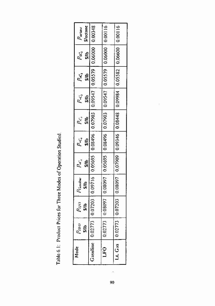
c

CO

o

o

H

(L>

O

NO

00

f^ ^

0 -c

/*! ^

^ £ CC 00

- ' ^ .Mk.

-^ 00

r " ^ <~N"" ri ^ 00

^ *T ._.

'O ;£ Ci, ^

V —

C^ 00

^ .. "2 -^

e O N

'

' S :£

!:> ^

' ^ -O

c£~ 00

ode

348

o o d o o o NO o d ON r--wo i/^

o d r-• ^

o d ro O ON r-o d vo OV "^ oo o d en ON VO wn O d o — r-OV O

d m O (N r-o d m r-r--fi o d

"o ;/:i

o

116

o o d o o o vo o d ON r-> i/^

wo O

d r-^ I/O Ov o d rn O OV r-o d NO OV -^ CO o d wo ON VO wo O d r OV o CO o d r Ov O CO o o

ro r-r r-i o d

O 15

116

o o d o o vo vo o d (N OO wo wo o d 'cr CO OV OV

o d CO ^ • ^

CO o d NO • ^

ro Ov o d Ov o ov

o d r ov O CO o d ro O Cl

r o d ro r-t^ Ol o d

;/3

6 •

90

6.1.3 Effect of disturbances on FCCU processing

Disturbances such as ambient and feed temperature changes have an effect on the

operation of the FCCU and on-line FCCU optimization. A drop in the ambient

temperature often allows an opportunity to process more gas oil. An ambient temperature

ramp was used to simulate daily temperature swings. Step changes in the gas oil feed

were introduced in another test case to study the effect of gas oil feed temperature on

FCCU optimization. On-line optimization test cases described in Tables 6.2 and 6.3 were

studied.

91

Table 6.2: Off-Line Optimization Matrix of Test Case Conditions.

Test Case

Case 1

Case 2

Case 3

Case 4

Case 5

Case 6

Operation Mode

Gasoline

Gasoline

LFO

LFO

Lt. Gas

Lt. Gas

Feed API

27

21

27

21

27

21

92

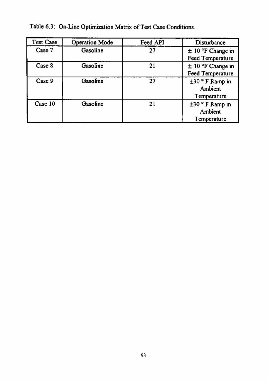
Table 6.3: On-Line Optimization Matrix of Test Case Conditions.

Test Case Case 7

Case 8

Case 9

Case 10

Operation Mode Gasoline

Gasoline

Gasoline

Gasoline

Feed API 27

21

27

21

Disturbance ± 10 °F Change in Feed Temperature ± 10 °F Change in Feed Temperature ±30 ° F Ramp in

Ambient Temperature

±30 ° F Ramp in Ambient

Temperature

93

CHAPTER 7

RESULTS AND DISCUSSION

In this work, a supervisory optimization routine was developed for a simulation of a

Model IV FCCU. The objective of the optimization routine was to supply process

variable setpoints to the nonlinear, multivariable controller that maximized unit

profitability while honoring all process constraints. A detailed yield model was used to

predict FCCU product yields based on process conditions, feed quality and ambient

conditions. To enhance the accuracy of the optimization setpoint predictions, process-

model mismatch was minimized by using adjustable parameters in the FCCU model. The

sensitivity of the optimization model to small changes in these adjustable parameters was

studied. The following section shows results from the off-line optimization studies, model

sensitivity analysis, and on-line optimization studies. Discussion of these results is also

provided.

7.1 Off-line Optimization Studies

Off-Hne optimization studies were accomplished using the FCCU optimization model,

ten lump yield optimization model, SQP constrained optimization algorithm NPSOL™

(Gill et al., 1986), and constant values for all the adjustable parameters. The purpose of

the off-line studies was to determine the relative increases in the optimization objective

fiinctions from predetermined base cases. The base cases shown in Table 7.1 used known

sub-optimal values for the regenerator temperature, riser temperature, gas oil

94

Table 7.1: Summary of Off-line Optimization Results: FCCU Optimization of Process from Arbitrary Setpoints. Constraints are defined in Table 4.1.

Case Study

API Mode

1.

2.

3.

4.

5.

6.

27 Gasoline

Base

21 Gasoline

Base

27 LFO

Base

21 LFO

Base

27 Lt. Gas

Base

21 Lt. Gas

Base

T °F reg ^

1265.0

1270.0

1265.0

1270.0

1265.0

1270.0

1265.0

1270.0

1265.0

1270.0

1265.0

1270.0

7;op

9 ^ . 0

994.0

990.6

990.0

993.0

994.0

990.5

990.0

993,9

994.0

990.5

990.0

F,,,lb/s

119.7

110.0

123.9

115.0

119.1

110.0

122.0

115.0

119.1

110.0

123.3

115.0

% ^ 2 . .

0.500

0.750

0.577

0.750

0.500

0.750

0.586

0.750

0.500

0.750

0.577

0.750

AObj.F

5.28 %

6.96 %

9.03 %

6.16%

8.57 %

6.56 %

Active

Constraints

1,2,4,5,9,13

2

1,9,10,13

1,2,4,5,9,13

2

1,9,10,13

1,2,4,5,9,13

2

1,9,10,13

95

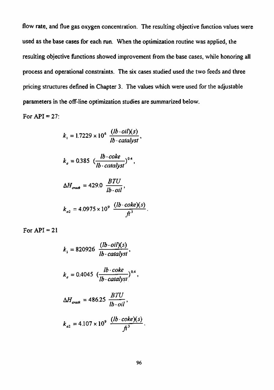
flow rate, and flue gas oxygen concentration. The resulting objective function values were

used as the base cases for each run. When the optimization routine was applied, the

resulting objective functions showed improvement from the base cases, while honoring all

process and operational constraints. The six cases studied used the two feeds and three

pricing structures defined in Chapter 3. The values which were used for the adjustable

parameters in the off-line optimization studies are summarized below.

For API = 27:

;^.= 1.7229x10- ^^^'-^^('\ lb • catalyst

^, = 0.385 ( "'•'°'" r . lb • catalyst

^cro^ = 429.0 BTU

lb • oil

9 {lb • coke)(s) k„, =4.0975x10

ft

For API = 21

(lb • oil)(s) k, =820926 ^^ ^ ,

lb' catalyst

lb coke 0 4

" lb-catalyst

BTU A ^ _ ^ = 486.25

"""^ Ib-otr

9 (lbcoke)(s) k , =4.107x10

ft

96

Frequency factors for the optimization yield model retained the values which are

summarized in Table 3.1. In all off-line optimization cases studied, improvements in unit

profitability were realized. Results from cases where the same feed was used showed

similar resuhs.

7.1.1. Off-line optimization results: Cases 1, 3, and 5

Off-line optimization Cases 1, 3, and 5 used a gas oil feed with an API gravity of 27.

The results of the optimization run showed an improvement in the optimization objective

function along with several active constraints. Riser temperature, regenerator

temperature, and flue gas oxygen concentration constraints were active along with the

firebox temperature constraint. The following paragraphs provide an explanation of the

off-line optimization results.

Setting the reactor temperature at its maximum allowable value had two beneficial

effects on the profitability of the FCCU. For the endothermic cracking reaction, increased

reactor temperature results in greater gas oil conversion. Since the octane value of the

gasoline produced in the FCCU is a function of conversion and reactor temperature, the

maximum reactor temperature also increased the octane value of the gasoline produced.

An increase of gasoline octane value results in a more valuable product.

Since the manipulated variable which directly controls the regenerator temperature is

the catalyst flow rate, one would expect that the regenerator temperature would be

minimized, as was observed in Cases 1,3, and 5. By increasing the catalyst flow rate, it

was possible to process more gas oil while maintaining medium severity conditions, which

97

are essential for gasoline production. Medium severity conditions refer to the catalyst-to-

oih;atio which maximizes the production of gasoline. A more rapid catalyst flow rate

removes energy from the regenerator, thus lowering the regenerator temperature.

The final major constraint encountered for Cases 1,3, and 5 was the firebox

temperature constraint. As stated in the previous paragraphs, it is beneficial to run the

FCCU at its maximum riser temperature. In order to maintain the maximum riser

temperature, energy must be supplied to the process to promote the endothermic cracking

reaction. This energy must come from the regenerated catalyst and the gas oil preheat

furnace. For Cases 1, 3, and 5, the gas oil feed used deposited a minimal amount of coke

on the catalyst during the cracking reaction. Since there was a relatively small amount of

coke on the spent catalyst, there was less coke to combust in the regenerator; therefore,

less energy could be liberated in the regenerator. The preheat furnace would be required

to add additional energy to the gas oil for the cracking reaction. The maximum amount of

energy which could be added to the gas oil feed was ensured by maximizing the preheat

furnace temperature until the temperature constraint was encountered.

The effect of pricing structure on the optimal process setpoints determined by the

optimization routine was not evident in Cases 1, 3, and 5. In each case, the production of

gasoline was maximized.

98

7.1.2. Off-line optimization results: Cases 2, 4, and 6

Cases 2, 4, and 6 used a gas oil feed which had a feed gravity of 21. The important

characteristic of this feed is that it deposits more coke on the catalyst during the cracking

reaction compared to the API=27 feed.

7.2 Sensitivitv Analvsis

The purpose of a sensitivity analysis was to determine the effect of model parameter

estimation error on the optimization algorithm performance. In this study, the percent

change in the calculated objective function caused by errors in parameter estimation was

determined. Off-line optimization was used in the sensitivity analysis study. Based on

process experience, worst case errors in parameter values were estimated and used in the

analysis. The sensitivity analysis was performed using the following method:

1. Perform a base case FCCU optimization using parameter values defined above

to obtain a reference objective function value.

2. Change the selected parameter using the optimizer model as shown in Table 7.2.

3. Perform off-line optimization using the optimizer model. Obtain the optimal

process setpoints predicted by the optimization algorithm.

4. Use the optimal setpoints obtained in Step 3 and perform optimization with the

original, error-free parameters.

5. Compare the objective function values obtained in Step 4 and Step 1.

The result obtained in Step 5 is a measurement of the lost economic opportunity caused by

model parameter uncertainty. Based on the results shown in Table 7.2, the

99

Table 7.2: Summary of Results from Sensitivity Analysis Study: The Effect of Parameter Uncertainty on Optimal Objective Value.

Change in Parameter

k^+1.5Vo

k^ -7.5 %

/:^+5.0%

k^.5.0Vo

AH^,^,+2.5%

^H^rack-2.5%

k^2 +5.0 %

k^2 -5.0%

T °F reg ^

1265.31

1265.31

1265.00

1265.00

1265.01

1265.0

1265.00

1265.00

rôp

994.00

993.95

992.6

994.00

993.97

994.00

992.60

994.00

Fî Ib/s

117.65

119.0

119.7

117.2

117.5

119.0

117.5

115.90

%o,.

0.500

0.500

0.500

0.500

0.500

0.500

0.500

0.500

A in Objf

-0.871 %

+0.00 %

-1.302%

-1.067%

-0.348 %

0.000 %

-2.482 %

-3.578%

100

optimization routine was most sensitive to inaccuracies in the frequency factor for the

depletion of oxygen reaction in the regenerator, k^^. One reason that inaccuracies in this

parameter have a marked effect on the optimization routine is that the parameter k^^

appears in an exponential term in the expression for the regenerator energy balance (see

expression 4-14). Since this term is always positive, small changes in the parameter will

always be amplified.

Another reason k^^ was a sensitive parameter was the quality of the regenerator

model. Simplifying modeling assumptions were made in the development of the

regenerator model. These assumptions included lumping of three reactions in the

combustion of coke from the spent catalyst into a single reaction, disregarding the dilute

phase above the catalyst bed, and modeling the gas flow through the regenerator as a plug

flow reactor. More accurate fluidized bed models, such as those described in Froment and

Bischoff (1990) and Levenspiel (1989), would provide a more accurate representation of

the regenerator. Using these models would also complicate the optimization algorithm

7.3 On-Line Optimization Studies

The on-line optimization studies considered the effect of process disturbances on the

FCCU process and optimization routine. Industrial FCC units encounter many process

disturbances which have a significant effect on the performance of the unit. To realize

optimal economic performance of a FCCU, at least two process constraints will be active.

The objective of the supervisory economic optimization routine is to consider the process

disturbances and determine if the process can be adjusted such that additional unit profits

101

can be realized. Often process disturbances will reduce the profitability of the FCCU. In

these cases, the supervisory optimization routine acts to minimize losses.

The current study considered two types of process disturbances:

1. Step Changes in the Feed Temperature Entering the Pre-heat Furnace,

2. Ambient Temperature Changes (30°F Ramp Change Over 3 Hours).

The study considered two feeds of different quality and used the Gasoline Mode pricing

structure. A summary of Test Cases is shown in Table 6.3. Results from the on-line

optimization study are shown below, along with a discussion of the optimization routine

performance.

The PMBC constraint controller used in this study was designed such that the gas oil

flow rate to the FCCU would always be maximized. This is important to remember when

reviewing the on-line optimization results. The on-line optimization routine only predicts

optimal setpoints and feeds them to the PMBC constraint controller. In reality, the

constraint controller reduces one of the degrees of freedom for process optimization: the

gas oil flow rate. When reviewing the gas oil flow rate optimization results, the actual gas

oil flow rate is always portrait. The gas oil flow rate predicted by the optimization

algorithm is also shown but is not used by the constraint controller. The gas oil flow rate

determined by the optimization algorithm should be close to the actual gas oil flow rate

value if the optimization model adequately describes the actual process.

102

7.3.1 On-line optimization studies: Test Case 7

For this case, the API=27 gas oil feed was processed in Gasoline Mode. Step changes

in the gas oil feed temperature were introduced at the following times:

1. For Simulation Time t < 10000 s, the Feed Temperature was 460 °F.

2. For Simulation Time 10000< t < 15000 s, the Feed Temperature was 450 °F.

3. For Simulation Time 15000< t < 20000 s, the Feed Temperature was 460 °F.

4. For Simulation Time t >20000 s, the Feed Temperature was 470 °F.

For all on-line cases studied, the process was initially operated at known sub-optimal

conditions. The first on-line optimization was performed at t=7600 s. The process

objective function value was determined on-line. The value of the sub-optimal objective

function prior to the first disturbance was used as the reference objective function value.

Figures 7.1-7.5 show the on-line optimization results when feed temperature

disturbances were considered. Figures 7.1 and 7.2 show that the optimization algorithm

suggested changes in the regenerator and riser temperature setpoints the first time the

optimization routine was called. The explanation behind these optimal setpoints is

described in the off-line optimization studies (see 7.1.1). Filtered setpoint values of 1265

°F for the regenerator, and 994 °F for the riser were fed to the PMBC controller. These

setpoints honored the respective temperature constraints. Recall that the minimum

regenerator temperature for complete combustion was 1265 °F, and the metallurgical

temperature limit on the riser was 995 °F. A one degree buffer for the maximum riser

temperature was used to ensure that temperature transients would not violate the riser

temperature constraint. The controller implemented these setpoints and pushed the

103

1275

- 1 2 7 0

"ro Q. E ^ 1265 f

2 I "ro I 0) I C ! (U j

2^1260 -OH

..-.

1255 3600 7200 10800 14400

Time (s) 18000 21600 25200

Regenerator Temperature — Optimal Setpoint

Fieure 7.1: Regenerator Temperature for Test Case 7: Disturbances at 10000, 15000, and 20000 seconds.

104

1005

1000 -

^ !

B 995 -ro U. 1

Q. -E o

a: ]

985 -

980 -3600 7200 10800 14400 18000 21600 25200

Time (s)

— Optimal Setpoint — Riser Temperature

Figure 7.2: Riser Temperature for Test Case 7: Disturbances at 10000, 15000, and 20000 seconds.

105

150

3600 7200 10800 14400 18000 Time (s)

21600 25200

Gas Oil Flow Rate — Optimal Value

Figure 7.3: Gas Oil Feed Flow Rate for Test Case 7: Disturbances at 10000, 15000, and 20000 seconds.

106

1.5

1.25 -

<D i O 1 ^ E, I i I ^0.75 V T

O 0.5 -<D _3 -I U- I

0.25 T

0 ^ ' ^ \ '• 1 • 1

3600 7200 10800 14400 18000 21600 25200 Time (s)

Flue Gas Oxygen Concentration — Optimal Setpoint

Figure 7.4: Flue Gas Oxygen Concentration for Test Case 7: Disturbances at 10000, 15000, and 20000 seconds.

107

8

0 ^ • (

3600 7200 10800 14400 Time (s)

18000 21600 25200

%Change in Objective Function

Figure 7.5: Percent Change in Objective Function for Test Case 7: Disturbances at 10000, 15000, and 20000 seconds.

108

process to the new operating temperatures. Subsequent optimizations held the

regenerator and riser temperatures at these optimal values regardless of feed temperature

disturbances.

The optimal gas oil flow rate prior to the first optimization run was set at 132 Ib/s.

After the first optimization cycle, the gas oil flow rate predicted by the optimizer was

approximately 115.0 Ib/s. Figure 7.3 shows the filtered implementation of the predicted

optimal gas oil flow rate. The actual gas oil flow rate as determined by the constraint

controller, after the initial optimization and prior to the first temperature disturbance, was

approximately 114.0 Ib/s. The predicted gas oil flow rate and the actual gas oil flow rate

were in agreement through subsequent optimizations for the remainder of the simulation.

Figure 7.4 shows the actual flue gas oxygen concentration and the optimal setpoint

predicted by the optimization algorithm. Throughout the entire simulation run, the

optimal flue gas oxygen setpoint was approximately 0.75 % even while encountering feed

temperature disturbances.

The effectiveness of on-line optimization is indicated in Figure 7.5: the percent change

in the objective fijnction value throughout the simulation run. Upon closer inspection of

Figure 7.5, the effect of the feed temperature disturbances can be seen. Prior to the first

optimization, the objective function value is at its reference value. After the first

optimization, a 5.0% change in the objective function was observed. The active

constraints after the process reached the new setpoints were the regenerator, riser, and

firebox furnace temperatures. At t= 10000 seconds, a -10 °F change in the feed

temperature was introduced. Since the preheat furnace was operating at its maximum

109

constraint prior to the temperature change, to maintain the riser temperature at 994 °F, the

gas oil feed rate had to be reduced. The dynamic response to the disturbance is apparent

in the actual gas oil feed rate and on-line objective fiinction value. The next optimization

cycle after the temperature disturbance, the predicted gas oil feed rate was reduced from

115.0 Ib/s to approximately 113.5 Ib/s. For this disturbance, the optimization model

recognized the disturbance and predicted a lower gas oil flow rate. Although it is not

perceptible from Figure 7.5, a -0.75% change in the on-line objective function was

observed. For disturbances at t=15000, and 20000 seconds, an increase in the feed

temperature was implemented. After each disturbance, additional gas oil processing

capability was predicted. An increase in feed temperature allowed the preheat furnace to

back off its constraint, while still maintaining the riser temperature at 994 °F.


Results from on-line optimization Test Case 8 are shown in Figures 7.6-7.10.

Temperature disturbances in the form of+10°F step changes were introduced into the feed

(feed quality of API=21) entering the preheat fijmace. When processing the API=21

gravity feed, the process encountered the maximum gas oil constraint (Constraint 3), and

the maximum catalyst flow rate constraint (Constraint 11). The feed conversion was

lower in the API= 21 feed when compared to the API=27 feed due to the higher amount

of aromatic compounds in the feed. The result of less gas oil feed conversion was less

energy required for the cracking reaction. Consequently, more gas oil feed could be

110

1275

^ 1 2 7 0 i a i 2 i Q- I

E i ^ 1265 7: o I To v_ 0)

c 0)1260 ,

CH !

- \ A ' /

1255 3600 7200 10800 14400

Time (s) 18000 21600 25200


Figure 7.6: Regenerator Temperature for Test Case 8: Disturbances at 10000, 15000, and 20000 seconds.

I l l

1005

1000 I

0)

B 995 T ro

E H 990 0) (A

985 +

980

3600

H V

-T *-

7200 10800 14400 Time (s)

18000 21600 25200

Optimal Setpoint — Riser Temperature

Figure 7.7: Riser Temperature for Test Case 8: Disturbances at 10000, 15000, and 20000 seconds.

112

150

140 T-

^ 1 3 0 ~ S "TO a: ^ 120 — o

O en 110 ro O

100 X

90 4— 3600 7200 10800 14400

Time (s) 18000 21600 25200


Figure 7.8: Gas Oil Feed Flow Rate for Test Case 8: Disturbances at 10000, 15000, and 20000 seconds.

113

1.5

1.25 r

2 1 ^

c Qi

510.75 X

O tn ro O 0.5 T 0)

U. 0.25

i\: l\ / V

iiv ^

0 + 3600 7200 10800 14400

Time (s) 18000 21600 25200


Figure 7.9: Flue Gas Oxygen Concentration for Test Case 8: Disturbances at 10000, 15000, and 20000 seconds.

114

10

r o . o c 3 u_ o >

o 03 ^ o _c « OJ c ro .c O V.O

r

8 - I

+

6 J

•'

4 T 1

' '

2 -

4

1)!) r '..''.'^V,A.\_..

0

3600 7200 10800 14400 Time (s)

18000 21600 25200


Figure 7.10: Percent Change in Objective Function for Test Case 8: Disturbances at 10000, 15000, and 20000 seconds.

115

processed. At 7600s, all of the responses show some ringing as the controller drives the

process to the optimal setpoints. To alleviate this ringing, the controller was detuned for

subsequent runs.

Figure 7.6 shows the regenerator temperature response during the on-line optimization

run when temperature disturbances were introduced into the gas oil feed entering the

preheat furnace. Initially, the regenerator setpoint was set at 1265 °F. After the first

optimization at 7600 s, the optimal regenerator setpoint was also 1265 °F. The optimal

regenerator setpoint remained at 1265 °F throughout the entire run. After the initial

temperature disturbance at t= 10000 s, the actual regenerator temperature value violated

the low temperature constraint of 1265 °F. The controller pushed the process variable

back towards 1265 °F for the remainder of the simulation

The riser temperature response for Test Case 8 is shown in Figure 7.7. The initial riser

temperature was set at 990 °F prior to the first optimization. After the first optimization

cycle (t=7600 s), the setpoint was filtered to its optimal value of 994 °F. The controller

pushed the riser temperature to 994 °F and held throughout the remainder of the

simulation run.

Figure 7.8 shows the response of the flue gas oxygen concentration for Test Case 8.

The optimal setpoint throughout the entire simulation was 0.75%. The actual oxygen

concentration showed ringing after the first optimization cycle, as the controller pushed

the process to the new optimal setpoints. The process variable ringing slowly subsided

after approximately 7600 s. As the simulation continued, the offset between the actual

oxygen concentration and the optimal setpoint was reduced.

116

The gas oil feed flow rate throughout the entire simulation run was constant at the

maximum gas oil feed flow rate constraint of 132 Ib/s as shown in Figure 7.9.

The percent change in the on-line objective function for Test Case 8 is shown in Figure

7.10. The average objective function value prior to the first optimization cycle was used

as a reference. After the first optimization cycle at t=7200 s, the on-line objective fijnction

value increased to approximately 6.5% of its original value. The fluctuations in the

objective function value after the first optimization cycle were caused by oscillations of the

flue gas oxygen value. It is important to note that constraints were being violated during

this transient period. Therefore, the peak in the objective function value at t=10800 s was

realized at the expense of constraint violation. Throughout the remainder of the

simulation, the objective function slowly decreased until it reached a constant value at

approximately 6.5% above the reference conditions. This corresponded to the regenerator

temperature and flue gas oxygen concentration approaching their respective optimal

setpoints, which were not in violation of process constraints.

In general, economic benefits were not realized in the face of the feed temperature

disturbances, since the gas oil feed was maximized throughout the entire simulation. A

small economic advantage may have been realized if the gas oil flow rate was reduced. A

reduction in the gas oil flow rate would create more severe cracking conditions, thus

increasing the yield of gasoline. This was not predicted by the optimization routine.

117


Test Case 9 studied the effect of ambient temperature changes on the performance of

the supervisory optimization routine. An ambient temperature ramp was implemented as

shown below:

1. For simulation time t < 10000 seconds, the ambient temperature was 75 °F,

2. For simulation time 10000< t < 20800 s, ambient temperature was

increased at a rate of 30 °F over the three hour period.

3. For simulation time 20800< t < 28800 s, the ambient temperature was

held constant at 105 °F.

4. For simulation time 28800< t < 39600 s, the ambient was reduced at a

rate of 30 °F over the three hour period.

Figures 7.11-7.15 show the on-line optimization results when the ambient temperature

disturbances were considered. Figures 7.11 and 7.12 show similar results that were

observed in previous optimization runs. The result of the first optimization cycle (at

t=7600 s) was to move the regenerator setpoint from 1270 °F to 1265 °F and the riser

temperature setpoint from 990 °F to 994 °F. The optimizer predicted these setpoint

changes for the same reasons described in 7.1.1. These optimal setpoint values were held

constant through ensuing optimization cycles throughout the entire run. The ambient

temperature disturbance had no affect on these optimal setpoints.

The optimizer predicted a gas oil flow rate of approximately 116 Ib/s after the first

optimization, as shown in Figure 7.13. The actual gas oil flow rate determined by the

constraint controller was approximately 115 Ib/s soon after the first optimization. During

118

1275

^ 1 2 7 0

"ro

Q. E ^ 1265

o "TO t _

a> c

11260

1255

3600 10800 18000 25200 Time (s)

32400 39600


Fieure 7.11: Regenerator Temperature for Test Case 9: Ambient Air Disturbances.

119

1005

^ 1 0 0 0

"TO

Qi

Q. 995 E o 0)

(5 990

985 3600 10800 18000 25200

Time (s) 32400 39600

Optimal Serpoint Riser Temperature

Figure 7.12: Riser Temperature for Test Case 9: Ambient Air Disturbances.

120

150

3600 10800 18000 25200 Time (s)

32400 39600

Gas Oil Flow Rate Optimal Setpoint

Figure 7.13: Gas Oil Feed Flow Rate for Test Case 9: Ambient Air Disturbances.

121

1.5 -

1.25 -

O

E 1 T

C

10.75 o ro O 0.5 o>

U.

0.25 T

3600 10800 18000 25200 Time (s)

32400 39600

Optimal Serpoint — Flue Gas Oxygen

Figure 7.14: Flue Gas Oxygen Concentration for Test Case 9: Ambient Air Disturbances.

122

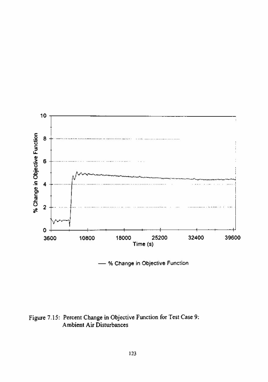
3600 10800 18000 25200 Time (s)

32400 39600

% Change in Objective Function

Figure 7.15: Percent Change in Objective Function for Test Case 9: Ambient Air Disturbances

123

the ambient temperature increase, the optimization routine predicted a 1.5 Ib/s increase in

the gas oil flow rate which was never realized by the actual gas oil flow rate. As the

ambient temperature decreased, the predicted gas oil flow rate returned to its pre-

disturbance value of approximately 116.0 Ib/s. This phenomenon was expected since the

combustion air blower was not constrained. An increase in the ambient air temperature

had the effect of adding thermal energy to the regenerator. In order to maintain the

regenerator temperature, the catalyst flow rate from the regenerator would have to

increase. Since the preheat furnace was constrained, the additional energy from the

catalyst helped to ease the firebox constraint condition. Consequently, additional gas oil

could be processed. The fact that the actual gas oil flow rate did not increase significantly

was due to the decrease in the flue gas oxygen setpoint. The decrease in the oxygen

setpoint was caused by modeling error and the sensitivity of the parameter used to

minimize process-model mismatch in the regenerator energy balance.

Figure 7.14 shows the response of the optimal flue gas oxygen setpoint and the

process variable value to the ambient air disturbance described above. The initial flue gas

oxygen setpoint was set at 0.75%, and retained the same value as a result of the initial

optimization. Ensuing optimization cycles predicted optimal setpoints which were less

than 0.75%. Since the combustion and lift air blower were not constrained, the optimal

value should have remained closer to the upper constraint value of 0.75% to process the

maximum amount of gas oil. Once again, this error can be attributed to the sensitivity of

the of the parameter used to minimize process-model mismatch in the regenerator energ>'

balance.

124

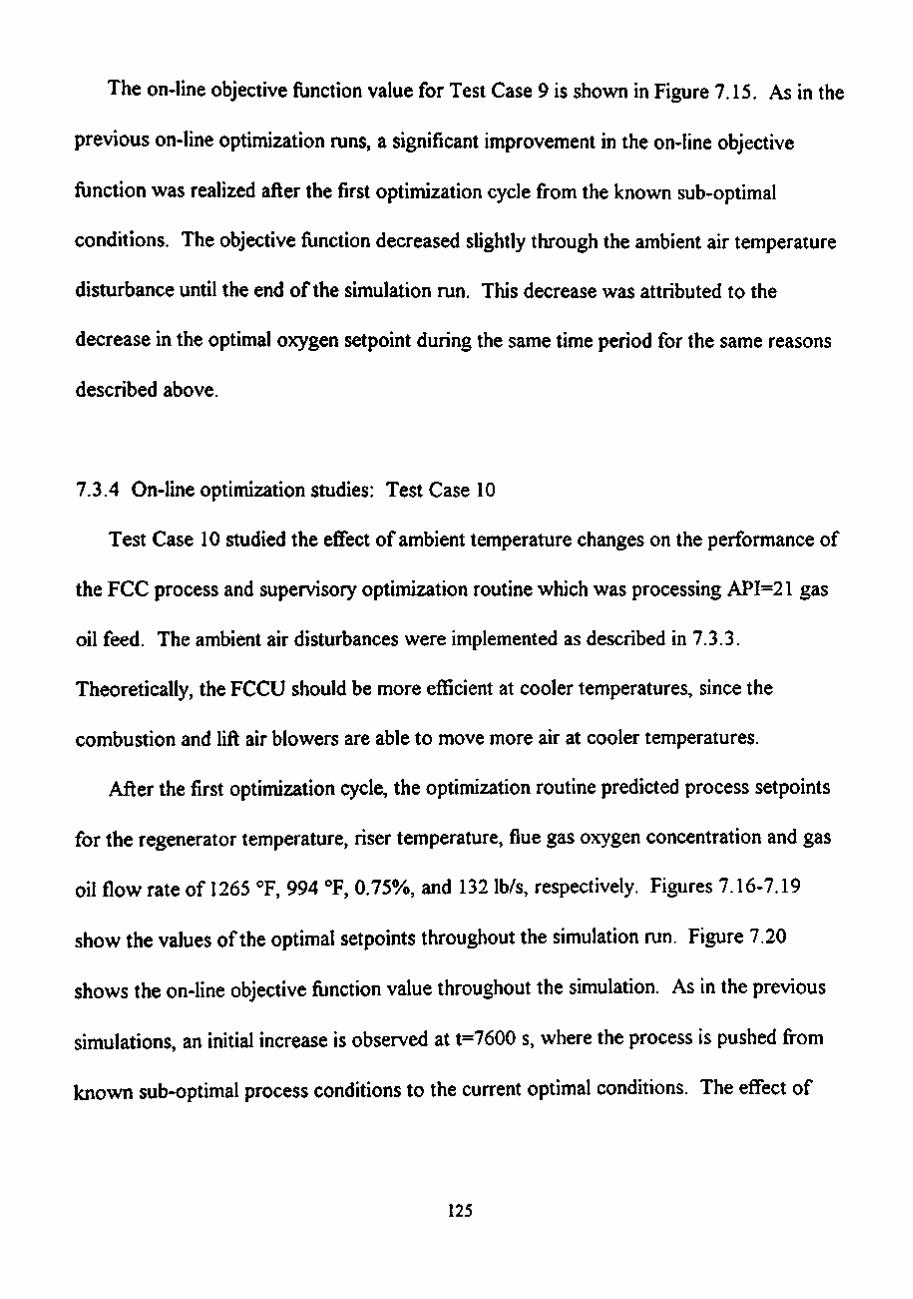
The on-line objective function value for Test Case 9 is shown in Figure 7.15. As in the

previous on-line optimization runs, a significant improvement in the on-line objective

function was realized after the first optimization cycle from the known sub-optimal

conditions. The objective fiinction decreased slightly through the ambient air temperature

disturbance until the end of the simulation run. This decrease was attributed to the

decrease in the optimal oxygen setpoint during the same time period for the same reasons

described above.


Test Case 10 studied the effect of ambient temperature changes on the performance of

the FCC process and supervisory optimization routine which was processing API=21 gas

oil feed. The ambient air disturbances were implemented as described in 7.3.3.

Theoretically, the FCCU should be more efficient at cooler temperatures, since the

combustion and lift air blowers are able to move more air at cooler temperatures.

After the first optimization cycle, the optimization routine predicted process setpoints

for the regenerator temperature, riser temperature, flue gas oxygen concentration and gas

oil flow rate of 1265 °F, 994 °F, 0.75%, and 132 Ib/s, respectively. Figures 7.16-7.19

show the values of the optimal setpoints throughout the simulation run. Figure 7.20

shows the on-line objective function value throughout the simulation. As in the previous

simulations, an initial increase is observed at t=7600 s, where the process is pushed from

known sub-optimal process conditions to the current optimal conditions. The effect of

125

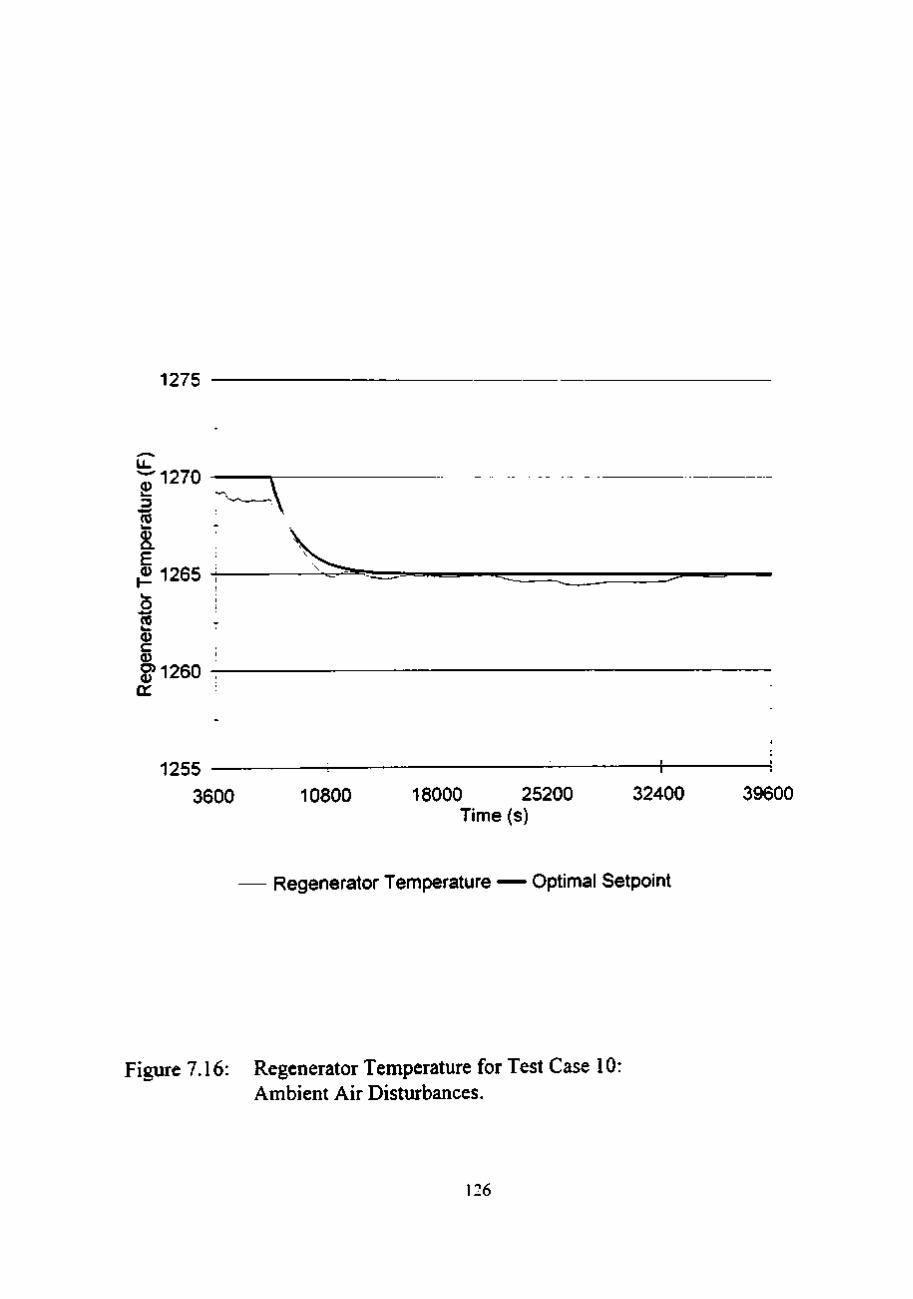
1275

- 1 2 7 0 I—

"TO

<D Q.

E ^ 1265 ^. o

"TO i—

c §^1260 Q:

^

1255 3600 10800 18000 25200

Time (s) 32400 39600


Figure 7.16: Regenerator Temperature for Test Case 10: Ambient Air Disturbances.

126

1005

1000

UL

0

3 995 ro CL

E 0)

0}

990

985

"v^

980 3600 10800 18000 25200

Time (s) 32400 39600

— Optimal Setpoint Riser Temperature

Figure 7.17: Riser Temperature for Test Case 10: Ambient Air Disturbances.

127

135

134

•S 133 ro a:

u. = 132 <n ro

O

131

130 3600 10800 18000 25200

Time (s) 32400 39600


Figure 7.18: Gas Oil Feed Flow Rate for Test Case 10: Ambient Air Disturbances.

128

1.5

1.25 — —

I '-c 5 0 75 ^-^-^ ^^^ -— TT^rr:=r. • -—••-•-•-" ^ - - ^ - r r ^ >% \J. I \J .. • ^^< —~ - - . . . ' —— X I

ro ! O 0.5 0)

L i - I

0.25

3600 10800 18000 25200 32400 39600 Time (s)


Figure 7.19: Flue Gas Oxygen Concentration for Test Case 10: Ambient Air Disturbances.

129

| 4

c

Ll_

0)

O •^2 0) O) c ro

x : O

3600 10800 18000 25200 Time (s)

32400 39600


Figure 7.20: Percent Change in Objective Function for Test Case 10: Ambient Air Disturbances.

130

increased ambient temperature can be seen by studying Figure 7.17. The optimization

routine predicted an increase in riser temperature setpoint during the ambient temperature

increase from 75 °F to 105 °F. After the ambient temperature reached a maximum value

of 105 °F (between 20800-28800 s), the optimization routine backed off the maximum

riser temperature constraint of 994 °F. By backing off this constraint, it was possible to

continue to process 132 Ib/s of gas oil feed. As the ambient temperature decreased from

105 °F to 75 °F, the optimization routine predicted optimal riser temperature setpoints

approaching 994 °F. Figure 7.20 shows the reduction in the on-line objective function

during the period of time when the ambient temperature was at a maximum, and the riser

temperature setpoint was less than 994 °F.

131

CHAPTER 8

CONCLUSIONS AND RECOMMENDATIONS

The main purpose of this work was to install a supervisory optimization routine to a

Model IV FCCU dynamic computer simulation. To accomplish this objective, it was

necessary to implement a detailed yield model to predict the range of products produced

by the FCCU. A steady-state FCCU model was developed to use with the nonlinear,

constrained SQP software package NPSOL' ' (Gill et al., 1986) to ensure maximum unit

profitability. To minimize mismatch between the FCC process and the optimization

model, model parameterization was implemented on-line. Different operating conditions

and product pricing structures were studied to demonstrate the effectiveness of the

supervisory optimization routine.

Off-line studies were performed to validate the yield and steady state optimization

models. Yield model validity was proved by comparing yield results to industrial data

found in the literature. FCCU steady state optimization model validation was

accomplished by comparing steady state simulation data with model results.

8.1 Conclusions

Based on the experience gained from this work, and discussions with industrial

experts, some conclusions can be drawn regarding the effectiveness of a supervisory unit

optimization routine. The following section describes a few areas which the control

engineer must be cognizant of when constructing a supervisory optimization routine.

132

As stated in previous sections, the performance of a supervisory optimization routine

is highly dependent on the quality of the model used to describe the process. In any

modeling project there is a trade-off between the model sophistication and computational

efficiency. For refinery optimization projects, such as optimization of a FCCU, it is

essential that rigorous models be developed for areas such as the regenerator, and yield

modeling. The resources invested in the development of accurate models are quickly

recouped, since small improvements in unit operation yield high economic benefits. In

summary, resources should be spent to develop high quality optimization models. With

the advent of high-speed computers, rigorous models can be solved in a time-efficient

manner.

This study considered only two parts of the entire optimization process as it is

performed in industry: parameterization and optimization. An example of an entire

optimization cycle is shown below.

1. Process steady-state identification.

2. Data reconciliation.

3. Model parameterization.

4. Economic optimization.

5. Review of optimal process conditions by process operators.

6. Implement optimal process variable targets

Each of these steps are essential for implementation of a successful supervisory

optimization routine. The most important step of the optimization cycle is Step 6.

Regardless of the level of modeling sophistication, it is very important that human element

133

is not removed from the optimization process. Often there are disturbances and objectives

which are not considered by the supervisory optimization routine. It is critical that the

process operator use information that the optimization routine is not aware of when

implementing process setpoints.

8.2 Recommendations

Many aspects of FCCU control and optimization were considered in this study.

However, there are still areas of modeling and optimization which could be studied.

These recommendations are listed below.

1. The effectiveness of process optimization is highly dependent on the quality of the

models used to simulate the process. In many cases, steady-state macroscopic

material and energy balances are adequate to capture the characteristics of the process.

Other situations call for more rigorous, distributed parameter models. In this study, it

was evident that the regenerator required a distributed parameter model to better

capture the behavior of the dense catalyst bed, the head space above the catalyst bed,

and the four reactions which occur in the regenerator. In fiiture process optimization

efforts, additional energy should be spent on constructing more rigorous models

where they are required.

2. The optimization techniques used in this study should be used for other processes.

The SQP algorithm NPSOL™ (Gill et al., 1986) is a very powerftil tool for solving

nonlinear, constrained optimization problems.

134

3. In this study, Newton's method was used solve the optimization model. The standard

method used in industry is open equation modeling. Open equation modeling, used

in conjunction with a SQP algorithm, allows for flexible modeling and a more robust

and efficient solution method. Model parameterization can be effected using the

same optimization model prior to each optimization cycle. Future modeling and

optimization work performed at Texas Tech should use open equation modeling.

Open equation modeling is critical for large refinery optimization problems.

4. The FCCU encounters countless disturbances. Future case studies could include

changes in upstream pressure from the vapor recovery unit, and the effect of catalyst

deactivation from metals in the gas oil feed.

5. Different product value scenarios should be investigated. For example, the value of

gasoline octane is quite dynamic, and is a function of conditions within and ex-ternal

to a particular refinery. This would be an interesting area for fiirther investigation.

6. The current multivariable process controller (PMBC) performs adequately for

processes that do not encounter multiple constraints. Intelligent constraint control for

complicated processes requires a model-predictive controller.

135

BIBLIOGRAPHY

Arbel A., Huang Z., Rinard I.H., Shinnar R., and Sapre A. Dynamics and Control of Fluidized Catalytic Crackers. 1. Modeling of the Current Generation of FCC's. Ind. Eng. Chem. Res. Vol. 34, pp 1228-1243, 1995.

Albus C , personal communications, October, 1994, Exxon Corporation, Lubbock, TX.

Blanding F.H. Reaction Rates in Catalytic Cracking of Petroleum. Ind. and Eng. Chem. Vol.45,No. 6, 1953.

Corma A., Juan J., Martos J., and, Soriano J.M. 8 ' Intemational Congress on Catalvsis (Berlin). Vol. E, pp 293-304, 1984.

Desai P.H., and Haseltine R.P., Advanced Catalyst Formulations Can Be Used to Boost Motor Octane Number of Gasoline, Oil and Gas Joumal, October 23, 1989, pp. 68-76.

[DMC] Corporation. Real-time Optimization and Control of Fluid Catalvtic Cracking Units, Cutler C, Houston, TX, 1990.

Froment G.F., and Bischoff K.B., Chemical Reactor Analvsis and Design, second edition, John Wiley and Sons, New York, NY, 1990, pp 576-584.

Gill P.E., Murray W., Saunders M.A., and, Wright M.H., Users Guide for NPSOL (version 4). A Fortran Package for Nonlinear Programming, Palo Alto, CA.

Hoffinan D., personal communications, October, 1994, [DMC] Corporation, Lubbock, TX.

Hindmarsh A.C., LSODE and LSODI, Two New Initial Value Ordinary Differential Equation Solvers. ACM SIGNUM Newsletter, 15, No. 15, 4 (1980), pp. 10-11,

136

Jacob S.M., Gross B., Voltz S.E., and Weekman Jr., V.W. A Lumping and Reaction Scheme for Catalytic Cracking. AIChE Joumal. Vol. 22, No. 4, pp. 701-713, July, 1976.

Jolin T.M., and Wojciehowski B.W. On Identifying the Primary and Secondary Products of Catalytic Cracking of Neutral Distillates. Joumal of Catalvsis. Vol. 37, pp. 240-250, 1975.

Lasdon L.S., and Warren A.D. A Survey of Nonlinear Programming Applications. Oper. Res. Vol. 28, No. 5, pp 34-50.

Levenspiel, O., The Chemical Reactor Omnibook, Oregon State Press, Corvallis, OR, 1989, Chapter 25.

Liguras D.K., Neurock M., Klein M.T., Stark S., Nigam A., Foley H.C., and Bischoff K.B., Monte Carlo Simulation of Complex Reactive Mixtures: A FCC Case Study, AIChE Symposium Series, Chuang K.C., Young G.W., Bensley R.M., editors, #291, volume 88, 1992.

Lin T.D.V. FCCU Advanced Control and Optimization. Hvdrocarbon Processing. Pages 107-114, April, 1993.

McFariane R.C., Reinemann R.C., Bartee J.F., and Georgakis C. Dynamic Simulator for Model rV Fluid Catalytic Cracking Unit. Computers and Chemical Engineering, Vol. 17, p 275, 1987

Maples R.E., Petroleum Refinery Process Economics, Penwell Publishing Company Tulsa, OK, 1993.

Murtaugh B.A., and Saunders M.A. Large-scale Linearly Constrained Optimization. Math. Program. Vol 14, pp 41-72.

Nace D.M., Voltz S.E., and Weekman, Jr., V.W. Application of a Kinetic Model for Catalytic Cracking: Effects of Charge Stocks. Ind. Eng. Chem. Process Develop., Vol. 10, No. 4, p 530-538,1971.

137

Nelson W.L., Yield Modeling, Oil and Gas Joumal, February 19, 1973, p. 86.

Reif H.E., Kress R.F., Smith J.S. How Feeds Effect Catalytic Cracking Yields. Petroleum Refiner. Vol. 40, No. 5, pp. 237-244, May, 1961.

Voorhies, A. Carbon Formation in Catalytic Cracking. Ind. and Eng. Chem. Vol. 37, pp. 318-322, 1945.

Voorhies A,, Jr., Kimberlin C.N., Jr., and Smith W.M., Oil and Gas Joumal, May 18, 1964, p. 108.

Wachtel S.J., Baillie L.A., Foster R.L., and Jacobs H.E., Oil and Gas Joumal, April 10, 1972, pp.104-107.

Weekman Jr., V.W., Nace D.M. Kinetics of Catalytic Selectivity in Fixed, Moving, and Fluid Bed Reactors. AIChE Joumal. Vol. 16, No.3, pp. 397-404, May, 1970.

White R.J. Effect of Feed Composition on Catalytic Cracking Yields. Oil and Gas Joumal, pp 112-116, May 20, 1968.

Winn F.W., Physical Properties by Nomogram, Petroleum Refmer, volume 36, no. 2, February, 1957, ppl57-159.

138

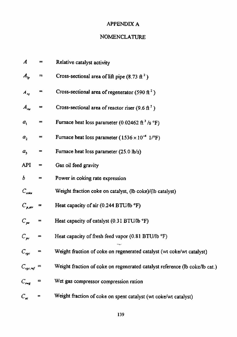
APPENDIX A

NOMENCLATURE

A = Relative catalyst activity

A,p = Cross-sectional area of lift pipe (8.73 ft ^)

A^^ = Cross-sectional area of regenerator (590 ft ^)

A^^ = Cross-sectional area of reactor riser (9.6 ft")

a, = Furnace heat loss parameter (0.02462 ft ^ /s °F)

^2 " Furnace heat loss parameter (1 .536x10^ 1/°F)

^3 = Furnace heat loss parameter (25.0 Ib/s)

API = Gas oil feed gravity

b = Power in coking rate expression

Q ^ Weight fraction coke on catalyst, (lb coke)/(lb catalyst)

C^^., = Heat capacity of air (0.244 BTU/lb °F)

C^, = Heat capacity of catalyst (0.31 BTU/lb °F)

C ^ = Heat capacity of fresh feed vapor (0.81 BTU/lb °F)

C^gc = Weight fraction of coke on regenerated catalyst (wt coke/wt catalyst)

^rgc.ref ~ Wclght fractlon of coke on regenerated catalyst reference (lb coke/lb cat.)

C^g = Wet gas compressor compression ration

Csc " Weight fraction of coke on spent catalyst (wt coke/wt catalyst)

139

c Wet gas production constant (0.0088438 Ibmol/lb feed °F)

C, = Wet gas production constant (0.00004 Ibmol/lb feed °F)

Conv = Weight fraction conversion of gas oil feed

Conv = Volume fraction conversion

Conv , ^^ = Base value conversion weight fracfion (0.55)

COR =

p.v

Catalyst-to-oil ratio (lb catalyst/lb gas oil feed)

Heat capacity of gas oil (0.81 BTU/lb oil)

C p.c

Heat capacity of catalyst (0.31 BTU/lb catalyst)

Activation energy for coke formation of catalyst (BTU/lb mole)

V

R

E F _

R

F,

F, oil

F svcn.lift

Activation energy of coke formation reaction (°F)

Activation energy for conversion of feed in three lump model ( F)

Activation energy ofcracking of lump k in ten lump yield model (BTU/lb)

Gas oil feed flow rate (Ib/s)

Air lift compressor inlet suction flow at base conditions (ICFM)

/ ,

/ ,

F,

F.

F.

PP

rgc

sucn.comb

sucn.lift

Octane value function used in objective function

Nonlinear valve flow rate function

Flow rate of regenerated catalyst (Ib/s)

Combustion air blower inlet suction flow (ICFM)

Lift air blower inlet suction flow (ICFM)

140

Fsucr^.wg = Wet gas compressor suction flow (ICFM)

Fsurge,cornb = Combustlon air blower surge flow (ICFM)

Fsurge,iift = Lift air blower surge flow (ICFM)

Fsurge.wg = Wet gas compressor surge flow (ICFM)

7V = Air flow rate into regenerator (Ib/s)

7\,, 1 = Flow through wet gas compressor suction valve (lb mole/s)

Fwg ^ Wet gas production in reactor (Ibmole/ s)

F5 = Flow of fuel to furnace (SCF/s)

Fg = Combustion air blower throughput (Ib/s)

F, = Combustion air flow to the regenerator (Ib/s)

Fg = Lift air flow to the regenerator (Ib/s)

Fj, = Wet gas flow to vapor recovery unit (lb mole/s)

hjp = Height of lift pipe (34 ft)

h^^ = Height of reactor riser (60 ft)

H^ = Wet gas compressor head

HFO = Weight fraction of heavy fiael oil (lump 1=1 to 4)

K = Light gas scaling constant

k = Frequency factor for conversion of feed in three lump model,

((lboil)(s)/lb cat)

k^f^ = Absorption of heavy aromatics rate constant (wt/lb catalyst)

141

cc

cp

comb

'lift

'N

k.O

'ol

11

12

L sp

Frequency factor for coking rate expression (lb coke/(lb cat.)(ft)(s))^''

Average ration of specific heats (1.39)

Combustion air blower discharge pipe flow resistance factor

(62.94 Ib/s psia)

Lift air blower discharge pipe flow resistance factor (5 Ib/s psia)

Basic nitrogen absorption coefficient (lbâsic Nitrogen, lb catalyst)

Frequency factor for cracking reaction of lump k ((lb oil)(s)/lb cat)

Frequency factor for the depletion of oxygen in the regenerator

((lb coke)(s)/ft')

Kinetic frequency factor for the formation of gasoline ((lb oil)(s)/lb cat.)

Combustion air blower vent valve flow rating (25 Ib/s psia)

Lift air blower vent valve flow rating (10 Ib/s psia)

Wet gas compressor suction valve flow rating (1.5 Ibmol/s psia)

Wet gas flare valve flow rating (0.5 Ibmol/s psia)

Level of calalyst in standpipe (ft)

LFO

MON

MONj

MW

O 2,ref

Weight fraction of Light Fuel Oil (lumps I = 5-8)

Motor Octane

Base Motor Octane Number (72.5)

Molecular weight (lb/lb mole)

Mole percent oxygen reference

142

Oj^g = Concentration of oxygen in regenerator stack gas (mole % )

Pî„ = Atmospheric pressure (14.7 psia)

Fbase ^ Combustion air blower base discharge pressure (psia)

Fbase,d ~ Lift air blower base discharge pressure (psia)

Pi,ip = Pressure at bottom of lift pipe (psi)

Pj = Product value used in the objecfive function ($/lb)

p^^ = Gasoline octane value used in objective function ($/octane value)

P^ = Pressure at bottom of reactor riser (psi)

P^j = Pressure at bottom of regenerator (psi)

P^^ = Discharge pressure of wet gas compressor to vapor recovery unit

(101 psia)

P^ = Combustion air blower suction pressure (psia)

P., = Combustion air blower discharge pressure (psia)

P3 = Lift air blower discharge pressure (psia)

P^ = Reactor pressure (psia)

F5 = Reactor fractionator pressure (psia)

Pg = Regenerator pressure (psia)

P.J = Wet gas compressor suction pressure (psia)

A , = Heat generatred from cracking (BTU/s)

p = Universal gas constant (10.73 ft psi/lbmol R)

143

R O N = Research Octane Number

sa = Actual speed of lift air blower (RPM)

' ' max = Maximum speed of the lift air blower (6100 RPM)

sa^.^ = Minimum speed of the lift air blower (5000 RPM)

sb = Base speed of the lift air blower (5950 RPM)

7 , = Temperature ofair entering regenerator (270 °F)

7 ,„ = Atmospheric temperature (75 °F)

7 = Octane base temperature (900 °F)

Tj^ = Furnace log mean temperature difference (°F)

7 = Temperature of reactor riser (°F)

7 ^ Average temperature in riser used in yield optimization model (°F)

T^^f = Basetemperatureofreactorriser energy balance (999 °F)

T^^g = Temperature of regenerator bed (°F)

^reg ref ^ Rcgcncrator reference temperature (944 k)

T; = Temperature of fresh feed entering furnace (°F)

T^ = Temperature of fresh feed entering reactor riser (°F)

7J = Furnace firebox temperature (°F)

UAf = Furnace overall heat transfer coefficient (25 BTU/s)

w = Superficial velocity of vapor in riser (ft/s)

w = Superficial velocity of catalyst in riser (fr/s)

144

w, - Terminal velocity of catalyst in riser (ft/s)

^cat,i,ft = Velocity of catalyst in the lift pipe (ft/s)

Vj.ji = Manipulated variable for llift air blower steam valve (0-1)

^s = Superficial velocity in regenerator (ft/s)

v,;, = Slip velocity (2.2 ft/s)

111 = Wet gas compressor suction valve position

^Koke "^ Weight fraction of coke produced

wt. = Weight fraction often lump species (lb/lb feed)

wt^^ = Weight fraction of light gas products

wtj^, = Weight fraction basic nitrogen (lb basic Nitrogen/lb catalyst)

W^ = Inventory of carbon in regenerator (lb)

W^^g = Inventory of catalyst in regenerator (lb)

W^^ = Inventory of catalyst in reactor riser (lb)

W^p = Inventory of catalyst in regenerator standpipe (lb)

= Height of cyclone inlet (45 ft)

Zjp = Height of lift pipe discharge ( l if t)

GREEK SYMBOLS

AH^^,^^ = Heat of combustion of coke (BTU/lb coke)

AH,,,,, = Heat of cracking (BTU/lb)

AHf, = Heat of combustion of fiimace fiiel (1000 BTU/SCF)

145

eye

AH,. = Heat ofcracking reaction oflumpi (BTU/lb mole)

^^/rae ^ Pressure drop across reactor main fractionator (9.5 psia)

AF^ = Pressure difference between regenerator and reactor (psi)

8 = Void fraction in riser

s^ = Effective void fraction in the regenerator dense phase bed

£j- = Apparent void fraction in the regenerator dense phase bed

pg = Volume fraction of catalyst in the regenerator

p, = Density of catalyst in the riser (lb/ft ^)

Pc dilute Density of catalyst in the dilute phase (lb/ft ^)

Pc dense "^ Dcnslty of catalyst in the dense bed (lb/ft ^)

p = Density of exit gas (Ibmol/ft ^ )

PJ.^ = Density of catalyst in lift pipe (lb/ft ^)

Pport = Settled density of catalyst (68 lb/ft' )

p = Average density of material in reactor riser (lb/ft )

p ^ = Vapor density at reactor riser conditions (0.57 lb/ft ^)

r„ = Residence time in riser (s)

(f, = Catalyst deactivation function (lb coke/lb catalyst)

^ = Feed coking tendency function

146

APPENDIX B

STEADY-STATE DATA

Table B.l: Steady-state simulation data used for the development of expression for gas oil feed conversion gravity API=27.

Run 1

2

3

4

5

6

7

8

9

10

Foil 120

120

120

120

120

120

120

120

120

120

Frgc 550.0

600.0

650.0

700.0

750.0

800.0

900.0

1000.0

1100.0

1200.0

Triser (ave.) 1007.1

1010.5

1013.5

1016.2

1018.7

1020.9

1024.8

1028.2

1031.0

1033.5

Conversion 0.5973

0.6266

0.6529

0.6765

0.6980

0.7174

0.7510

0.7792

0.8030

0.8232

147

Table B.2: Steady-state simulation data used for the development of expression for gas oil feed conversion gravity API=21.

Run

1

2

3

4

5

6

7

8

9

10

Foil

120

120

120

120

120

120

120

120

120

120

Frgc

850.0

900.0

950.0

1000.0

1100.0

1200.0

1300.0

1400.0

1700.0

2000.0

Triser (ave.)

1022.9

1024.9

1026.6

1028.2

1031.0

1033.7

1035.7

1037.6

1042.2

1045.6

Conversion

0.5475

0.5643

0.5820

0.5982

0.6270

0.6540

0.6774

0.6985

0.7501

0.7893

148

Table B.3: Correlation data for Butane based on work by Gary and Handwerk (1984).

Volume % Conversion

60

70

80

60

70

80

60

70

80

60

70

80

60

70

80

Feed API

19

19

19

21

21

21

23

23

23

25

25

25

27

27

27

Volume % Butane

1.80

2.20

2.6

1.70

2.10

2.50

1.60

2.00

2.40

1.46

1.83

2.20

1.32

1.66

1.99

149

Table B.4: Correlation data for Butylenes based on work by Gary and Handwerk (1984).

Volume % Conversion

60

70

80

60

70

80

60

70

80

60

70

80

60

70

80

Feed API

19

19

19

21

21

21

23

23

23

25

25

25

27

27

27

Volume % Butylenes

5.96

7.47

8.98

5.87

7.36

8.85

5.78

7.26

8.73

5.66

7.12

8.58

5.54

6.98

8.43

150

Table B.5: Correlation data for i-Butane based on work by Gary and Handwerk (1984).

Volume % Conversion

60

70

80

60

70

80

60

70

80

60

70

80

60

70

80

Feed API

19

19

19

21

21

21

23

23

23

25

25

25

27

27

27

Volume % i-Butane

3.84

4.74

5.64

3.98

4.93

5.89

4.12

5.13

6.14

4.26

5.33

6.39

4.41

5.53

6.65

151

Table B.6: Correlation data for Propane based on work by Gary and Handwerk (1984).

Volume % Conversion

60

70

80

60

70

80

60

70

80

60

70

80

60

70

80

Feed API

19

19

19

21

21

21

23

23

23

25

25

25

27

27

27

Volume % Propane

1.80

2.35

3.00

1.80

2.35

3.00

1.80

2.35

3.00

1.80

2.35

3.00

1.80

2.35

3.00

152

Table B.7: Correlation data for Propylene based on work by Gary and Handwerk (1984).

Volume % Conversion

60

70

80

60

70

80

60

70

80

60

70

80

60

70

80

Feed API

19

19

19

21

21

21

23

23

23

25

25

25

27

27

27

Volume % Propylene

3.40

3.90

4.80

3.80

4.60

5.60

4.40

5.20

6.40

4.60

5.60

7.20

5.00

6.00

7.60

153

Table B.8: Correlation data for < Cj'^ gases based on work by Gary and Handwerk (1984).

Volume Vo Conversion

60

70

80

60

70

80

60

70

80

60

70

80

60

70

80

Feed API

19

19

19

21

21

21

23

23

23

25

25

25

27

27

27

Weight % <C,'s

3.65

5.20

7.60

3.40

4.80

6.85

3.00

4.20

5.80

2.40

3.60

4.80

2.10

2.80

4.00

154

Table B.9: Sample of Steady State Data used for Catalyst Inventory Correlation.

FT

68 68 68 68 69 69 69 69 70 70 70 70 71 71 71 71 72 72 72 72 73 73 73 73 74 74 74 74

FRGC

600 650 675 700 600 650 675 700 650 700 725 750 675 700 725 750 675 700 725 750 675 700 725 750 675 700 725 750

WRIS

1526.9 1648.8 1709.4 1769.6 1527 1649 1709 1770 1649 1770 1830 1890 1709 1770 1829.9 1890 1710 1770 1830 1889 1710 1770 1830 1890 1710 1770 1830 1890

W R E G

285841 284014 282960 282069 284998 283147 282060 281161 282660 280717 279932 279291 281030 279876 279066 278378 280154 278980 278149 277443 279278 278085 277235 276510 278401 277191 276323 275582

WR

92570 93031 93423 93628 93593 94083 94514 94722 94696 95293 95377 95303 95795 96299 96415 96394 96835 97362 97503 97505 97872 98420 98583 98606 98904 99471 99656 99698

WSP

257.1 1622.8 2285.2 2978 77.7 1437 2094 2785 1313 2658 3359 4074 1843 2494 3188 3896 1678 2326 3016 3721 1519 2164 2850 3552 1363 2006 2689 3388

155

APPENDIX C

SUMMARY OF COMPUTER PROGRAMMING

A brief description of each subroutine created and used in the FCCU simulation

and optimizafion routines is offered below. For a complete description of the original

FCCU simulation, refer to Khandalekar (1993).

C l SubroutineYLDTEN

The ten lump FCC yield model used in the simulation is located in the subroutine

YLDTEN2. The subroutine contains twelve spatial differential equations which describe

the differential material balances of each lumped species, the differential formation of coke

on catalyst, and the differential energy balance. These differential equations are evaluated

using the integration package LSODE (Hindmarsh, 1980). Subroutines FEX, RISER,

LIGHTS, and OCTANE are called by YLDTEN2. These subroutines are only called by

the subroutine YLDTEN2.

C.2 Subroutine NPOPT

This subroutine is used as the driver program for the SQP software package

NPSOL"^^ (Gill, et al., 1986). The subroutine contains economic information on the

FCCU products, FCCU constraint information, and program parameters which are used in

the SQP routine. The economic objective fiinction is contained in two subroutines which

156

are called by the SQP routine. For more information regarding the software package

NPSOL' ' (Gill, et al., 1986) the reader is referred to the software documentation.

C.3 Subroutine NPPAR

This subroutine is used as the driver program for the SQP software package

NPSOL""^ (Gill et al., 1986). This subroutine contains information on the parameters used

to parameterize the ten lump optimization yield model YLDOPT, and program parameters

which are used in the SQP routine. The yield model objective function is contained in two

subroutines which are called by the SQP routine. For more information regarding the

software package NPSOL"™ (Gill et al., 1986) the reader is referred to the software

documentation.

C.4 Subroutine NEWOPT

The subroutine NEWOPT is the steady-state FCCU optimization model.

Newton's method is called from this subroutine to evaluate six nonlinear differential

equations. The Jacobian is calculated using numerical approximations. Twelve additional

FCCU variables were calculated explicitly in this subroutine. The expressions used in this

subroutine are describe in the main text of this thesis.

C 5 Subroutine YLDOPT

YLDOPT contains ten differential equations which are used to describe the

differential material balances for each kinetic lump in the ten lump model. This subroutine

157

assumes that the temperature and coke concentration on the catalyst are constant across

the riser. This subroutine is called by subroutines NPPAR for parameterization, and

NPOPT for economic optimization. Subroutines FEXO, LIGHTSO, RISERO, and

OCTANEO are called by the subroutine YLDOPT.

C.6 Subroutine YLDPAR

See description of YLDOPT.

158

FCCU Process S imu la t ion

1 Subrou t ine NPOPT

Call NPPAR ^,—

Call NPSOL

Return to FCCU S imu la t i on

with Opt ima l Se tpo in ts

r Subrou t ine NPPAR

i t Subrou t ine NPSOL

I f Subrou t ine YLDOPT

• S u b r o u t i n e N P S O L ^

I Subrou t ine NEWOPT

I Subrou t ine YLDOPT

Figure C l : Flow Diagram of Optimization Algorithm

159

PERMISSION TO COPY

In presenting this thesis in partial fulfillment of the

requirements for a master's degree at Texas Tech University or

Texas Tech University Health Sciences Center, I agree that the Library

and my major department shall make it freely available for research

purposes. Permission to copy this thesis for scholarly purposes may

be granted by the Director of the Library or my major professor. It

is understood that any copying or publication of this thesis for

financial gain shall not be allowed without my further written

permission and that any user may be liable for copyright infringement.

Agree (Permission is granted.)

Me,. M~ ^r^W C> , \^'\C

Student's Signature Date

Disagree (Permission is not granted.)

Student's Signature Date

Documents

A THESIS the Requirements for - TDL