Embed Size (px)
Citation preview
JOURNAL OF MULTIVARIATE ANALYSIS 8, l-29 (1978)
A Third-Order Optimum Property of the Maximum Likelihood
Estimator
J. PFANZAGL AND W. WEFELMEYER
Mathematisches Institut der Universitiit K&z, K&t, West Germany
Communicated by L. K. Schmetterer
Let 8’“’ denote the maximum likelihood estimator of a vector parameter, based on an i.i.d. sample of size n. The class of estimators 0’“’ + n-r q(P)), with q running through a class of sufficiently smooth functions, is essentially complete in the following sense: For any estimator T(“) there exists q such that the risk of B(“) + n-l q(V) exceeds the risk of T’“) by an amount of order o(n-‘) at most, simultaneously for all loss functions which are bounded, sym- metric, and neg-unimodal. If q* is chosen such that 0’“) + n-r q*(W) is un- biased up to o(n-I/*), then this estimator minimizes the risk up to an amount of order o(n-‘) in the class of all estimators which are unbiased up to ~(a-‘/~).
The results are obtained under the assumption that T(“) admits a stochastic expansion, and that either the distributions haveroughly speaking-densities with respect to the Lebesgue measure, or the loss functions are sufficiently smooth.
1. SUMMARY
Let PO I&, 8 E 8, with 6 C W be a parametrized family of probability
measures. The problem is to estimate 0 on the basis of n i.i.d. observations. It is well known that a m.1. (maximum likelihood) estimator P) for the sample size rz is as. (asymptotically) maximally concentrated about the true parameter value in the sense that for any other estimator PI,
~~ydq~(n) - e) E cl < ~,q~ye(fi) - e) E cl + o(no) (1.1)
for every measurable set C which is convex and symmetric about the origin. This was proved by Kaufman (1966, p. 157, Theorem 2.1) under the assump-
tion that the distribution of n’/“(P) - 0) under Pen converges to some limiting distribution locally uniformly in 0. Another proof of the same result was given by Hajek (1970, p. 328, Corollary 1).
Received June 15, 1977.
AMS 1970 subject classifications. Primary 62FlO; Secondary 62CO7, 62E20, 62F20. Key words and phrases. Asymptotic theory, Edgeworth-expansions, higher-order
efficiency, complete classes, maximum likelihood estimation, unbiasedness.
1 0047-259X/78/0081-0001$02.00/0
Copyright 0 1978 by Academic Press, Inc. All rights of reproduction in any form reserved.
2 PFANZAGL AND WEFELMEYER
In this paper we shall further investigate the differences between as. efficient estimators (i.e. between estimator-sequences Ten), n E N, for which equality holds in (1.1)).
For technical reasons we restrict our considerations to the class 2 of all as. efficient estimator-sequences admitting a stochastic expansion (3.1).
The first result: For any estimator-sequence Vn), n E N, in Z there exists a vector-valued function q: 0 + RP such that the Edgeworth-expansions of the distributions of n112(@n) + n-l q(tYn)) - 0) and &2(T(n) - 0) coincide up to ~(n-l/~). This function q is uniquely determined by the requirement that the two estimator-sequences have up to o(&/~) the same bias.
As a particular consequence of this result we have that the n-i/2-terms of the Edgeworth-expansions agree for any two estimator-sequences in 2 which are efficient and as. unbiased of order ~(n-l/~). In other words: First-order efficiency implies second-order efficiency1 for estimator-sequences in 2 which are as. unbiased of order ~(n-l/~).
This result on second-order efficiency still leaves us with the possibility that as. efficient estimator-sequences are incomparable if the n-l-terms of their Edgeworth-expansions are taken into account. Such apprehensions do not materialize if the estimators are compared on the basis of their concentration, Po~{?w(T(~) - e) E C}, on measurable sets C which are convex and symmetric about the origin, or more generally on the basis of their risk, Psn(L(n1/2(T(“) - e))), incurred under measurable loss functions L which are nonnegative, bounded, neg-unimodal and symmetric about the origin.
More specifically, our main result (Theorems 1, 1’) is that for any such loss function,
PoyL(d/2(e(n) + n-lq(ey - 8)))
< ~~y~(d/2p) - e))) + o(n-l).
Hence the class of estimator-sequences of the form 8rn) + n-lq(@)), n E N, with q sufficiently smooth, is as. essentially complete of order o(&) in 2.
If we eliminate the bias of the m.1. estimator (see Corollaries 1, l’), i.e. if we choose q* such that t9(n) + dq*(P)), 71 E N, is as. unbiased of order o(n-lj2), then this estimator-sequence is optimal in the class of all estimator-sequences in 2 which are as. unbiased of order o(+/~), in the following sense: It minimizes the risk up to o(n-l) with respect to all measurable loss functions which are nonnegative, bounded, neg-unimodal and symmetric about the origin.
* For properties related to the second term of the as. expansion of the covariance matrix of an estimator-sequence, C. R. Rao (1961, p. 538; 1962, p. 49; 1963, p. 200) coined the term “second-order efficiency.” This term is also used by J. K. Ghosh and K. Subramanyam (1974, p. 335). The as. expansion of the covariance matrix proceeds in powers of n-r, whereas the as. expansion of the distribution of a standardized estimator-sequence proceeds in powers of ~‘1~. Hence in our more general set-up it appears natural to use the term “third-order efficiency” for what corresponds to Rao’s “second-order efficiency.”
MAXIMUM LIKELIHOOD ESTIMATOR 3
A corresponding optimum property also holds for other estimators, e.g. the
Bayes estimators (see Remark 3.24). The results mentioned so far hold under a Cramer-type continuity condition
referring to the functions occurring in the stochastic expansion (3.1) of the estimator-sequence. Roughly speaking, this condition excludes discrete proba- bility measures. If we restrict our considerations to sufficiently smooth loss functions, then the Cramer-type continuity condition can be dispensed
with. Corresponding results for tests under the Cramer-type continuity condition
are presented in Pfanzagl and Wefelmeyer (1977, p. 11, Theorem 1, and p. 15, Theorem 2).
The notations are collected in Section 2; Section 3 presents the results. The
regularity conditions are formulated in Section 4. Section 5 contains technical lemmas two of which on symmetric and unimodal functions may be of inde- pendent interest. The proof of the main theorem is given in Section 6.
2. NOTATIONS
Let (X, J&‘) be a measurable space and Pe / &, tJ E 0, with open 0 C [WP, a family of p-measures (probability measures). Let Pe* 1 zZo2” denote the n-fold
independent product of identical components Pe I.&. Throughout, functions f: X x 0 * --f Iw are always assumed measurable in x
for each fixed 0 E 0. A function f will be called d$fere&zbZe if it is differentiable in 8 for every x E X; greek superindices denote derivatives with respect to
corresponding components of 8. In the following, we assume that unspecified functions f are standardized such that P,(f(., 0)): = sf(x, f?) P,(dx) = 0. Furthermore,
J<(Xl ,..., 4, 0) := n-112 f (fb~, 0) - qf(., 0))).
Let P I&’ be a p-measure, fi X+ R, and g: X-+ [wk with P(g) = 0 and positive definite covariance matrix I’ : = P(gg’). Then f / g denotes the regress&
residual with respect to P off on g:
f I g := f - P(f) - P(fg’) r-55
For typographical reasons we write p and p 1 g instead of fz and fG We shall use the following convention. If in an additive term an index occurs
at least twice, this means summation over all values of the index set. For a function G(u, o, 0) on [WP x UV x 0, parenthesized greek and roman
type superindices denote derivatives with respect to corresponding components
4 PFANZAGL AND WEFELMEYER
of u and v, respectively; nonparenthesized greek superindices denote derivatives with respect to corresponding components of 8, i.e.:
G(4 :=.&G, a
G(i) := SG, 2
Gv=$G. (I
Define
a dP, 1 d z.(.,e):=~(dP,/~)i,,.
For instance,
Finally, let
L&q = ptp(*, 0) I’(*, m
Lasy(e) = pdwt, 0.
L := &,8)~,8=1,..., 2, 9 A :=L-1, and A, := A,,P,
where A,, are the elements of (1. Wk denotes the Bore1 algebra of W, and gk the class of all convex sets in Wk.
$jk denotes the class of all functions h: W + [--I, I] admitting continuous partial derivatives up to the third order which are bounded by 1.
For a vector-valued function f: X -+ Rk let P *f 1 Wn denote the induced measure, defined by P* f (B) := P(f-lB), BE&?~.
v,r denotes the Lebesgue density of the multivariate normal distribution Nz with mean vector zero and covariance matrix 2.
2.1. DEFINITION. Let jJ be a class of measurable functions f: Rk -+ R.
A sequence pe w j &P 0 E 0, n E N, of families of signed measures is approximated , up to o(n-s/a), uniformly on 3 [and locally uniformly in 81, by a sequence vfr 1 ak, 6 E 8, 71 E N, of families of signed measures if uniformly for f E 5 [and locally uniformly for e E 91
p?‘(f) = l&f) + 0(,-q.
A class of sets in ak is identified with the corresponding class of indicator
functions.
2.2. DEFINITION. For a sequence of functions fn: X* x 8 + R, n E N,
MAXIMUM LIKELIHOOD ESTIMATOR 5
we write f+, = Z,,(s) if for every 6 E 8 there exist a neighborhood U, of 8 and a constant u > 0 such that uniformly for 8’ E U, and \I 0” - 8’ [I < n-llla log rz,
P;*{lfn(*, q > (log n>(i} = o(?z-~‘s).
The relationf, = g, + n-r&(~) is defined as nr(fn - g,) = Z,(S).
3. THE RESULTS
We consider estimator-sequences T @I: X” -+ KY’, 12 E N, admitting a stochastic expansion of the form
#(T(@ - 8) = x + d2Q1(x,f, *) + &Q,(Ti, f, j, *) + r3i2Zn(2) (3.1)
with f T= (fr ,..., fG)‘: X x 8 -+ R*, g = (gr ,..., g7)‘: X x 8 -+ II?, Qr: [WP x IF@ x 0 -+ R, Q2: W’ x W x IFi+ x 0 + R.
Whenever (3.1) is used, the following convention is understood. For 0 E 9, the components of (A(., e), f(+, 0), g(., 0)) are linearly independent
under P, . The components of f(*, 0) are PB-uncorrelated to h(*, e), and the components of g(., 8) are P,-uncorrelated to h(., 0) and f(., 0). Furthermore, f(*, 0) constitutes a base under P, for the regression residuals &s(., 0) - pdv~(., 4)) I w, a and g(; 0) constitutes a base under PO for (A?(-, 0) - R&?‘( -, 4)) I (W, 4, fc, 0)) and (.A% 0) - pdfi% 9) I (C 0 fc, 0 where a,fi,y = l,..., p, i = l,..., Q.
Let 2 [resp., %‘I denote the class of all estimator-sequences T(“), n E N, admitting a stochastic expansion (3.1) for which the following regularity con- ditions are fulfilled. The vector (X, f, g) fulfills Condition C. [This assumption is not required for estimator-sequences in %‘.I Furthermore, (h,f, g) fulfills Condition U4; its components fulfill Condition D. The functions Qr=, Qfi, QL , Qza fulfill Condition B for OL, p = l,..., p; i = l,..., p, [For 2’ in addition: Ql(O, et, 0) and Q&l ~1, w, 0) admit continuous partial derivatives up to the third order with respect to v and w which are bounded by polynomials, locally uniformly in e.]
3.2. DEFINITION. An estimator-sequence T(“): X” -+ [WP, n E N, is ~(n-“/~)- cmistmt if for (Y = l,..., p,
n1/2(TF) - e,) = Z,(S).
3.3. DEFINITION. An estimator-sequence 0(n): Xfl -+ I&‘, n E N, is us. m.Z. (asymptotically maximum likelihood) of order n-?Z,(s) if it is o(n-8/2)-consistent and if for a = l,...,p,
by-, e(n)) = d,(+
6 PFANZAGL AND WEFELMEYER
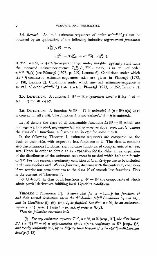
3.4. Remark. As. ml. estimator-sequences of order n-(S+1)/2Zn(s) can be obtained by an application of the following inductive improvement procedure:
T&j’ : = T[,nl,, + r~-l’~h( a, T&,).
If T@), n E N, is o(n-s/2)-consistent then under suitable regularity conditions the improved estimator-sequence T&(*, T(“)), n E N, is as. ml. of order B-(~+~)/~Z~(S) (see Pfanzagl (1973, p. 249, Lemma 6). Conditions under which o(n-8/2)-consistent estimator-sequences exist are given in Pfanzagl (1972, p. 190, Lemma 2). Conditions under which any m.1. estimator-sequence is as. ml. of order K@+~)/~Z~(S) are given in Pfanzagl (1973, p. 252, Lemma 7).
3.5. DEFINITION. A function h: W -+ Iw is symmetric about z if h(z + x) = h(.z - x) for all x E Iw”.
3.6. DEFINITION. A function h: W ---f Iw is unimodal if {x E (w”: h(x) > Y} is convex for all Y E R. The function h is neg-unimodal if --h is unimodal.
Let L3 denote the class of all measurable functions L: W + Iw which are nonnegative, bounded, neg-unimodal, and symmetric about zero. Let !S’ denote the class of all functions in !i! which are in c$jp for some c > 0.
In the following Theorem 1, estimator-sequences are compared on the basis of their risks with respect to loss functions in !& The class 2 contains also discontinuous functions, e.g. indicator functions of complements of convex sets. Hence in order to obtain an as. expansion for the risks, an as. expansion of the distribution of the estimator-sequences is needed which holds uniformly on VP. For this reason, a continuity condition of Cramer-type has to be included in the assumptions on%. We can, however, dispense with the continuity condition if we restrict our considerations to the class 2’ of smooth loss functions. This is the content of Theorem 1’.
Let D denote the class of all functions 4: Iwp -+ W the components of which admit partial derivatives fulfilling local Lipschitz conditions.
THEOREM 1 [Theorem 1’1. Assume that for (Y = l,...,p the functions l= and their partial derivatives up to the third-order fuljll Conditions L, and IWe , and let Conditions (i), (ii), (iii), I3 be ful$lled. Let W, II E N, be an estimator- sequence in 2 [resp. 2’1 which is as. m.l. of order n-V,(2).
Then the following assertions hold.
(i) For any estimator-sequence Ttn), n E N, in 2 [resp., 2’1, the distributzon POn c n1/2(T(“) - 0) is approximated up to o(n-l), unzformly on 59’ [resp., jjp] and locally unsformly in 8, by an Edgeworth-expansion of order o(n-I) with Lebesgue density (6.18).
MAXIMUM LIKELIHOOD ESTIMATOR 7
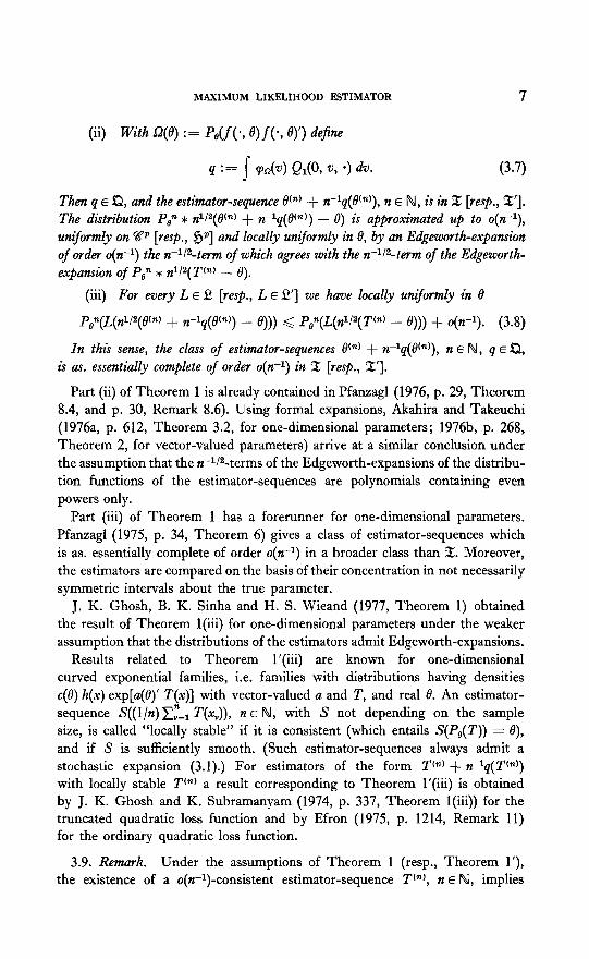
(ii) With Q(0) := P,(f(., e)f(*, 0)‘) define
(3.7)
Then q E 8, and the estimator-sequence 19 cn) + n-lq(O(“)), n E N, is in Z [resp., 211. The distribution POn * nllz(W + n-lq(fW) - 0) is approximated up to o(n-l), uniformly on %?’ [resp., !$I and locally uniformly in 0, by an Edgeworth-expansion of order o(n-I) the n-i/2-term of which agrees with the r1i2-term of the Edgeworth- expansion of Psn * n112( T(%) - 6).
(iii) For every L E !i? [resp., L E !i?‘] we have locally uniformly in t9
poyqnlye(~) + n-lq(W) - 6))) < Pen(L(n112(T(n) - 0))) + o(n-l). (3.8)
In this sense, the class of estimator-sequences W) + n-lq(W)), n E N, q E Q
is as. essentially complete of ordu o(n+) in 2 [resp., 2’1.
Part (ii) of Theorem 1 is already contained in Pfanzagl (1976, p. 29, Theorem 8.4, and p. 30, Remark 8.6). Using formal expansions, Akahira and Takeuchi (1976a, p. 612, Theorem 3.2, for one-dimensional parameters; 1976b, p. 268, Theorem 2, for vector-valued parameters) arrive at a similar conclusion under the assumption that the n-l12-terms of the Edgeworth-expansions of the distribu- tion functions of the estimator-sequences are polynomials containing even powers only.
Part (iii) of Theorem 1 has a forerunner for one-dimensional parameters. Pfanzagl (1975, p. 34, Theorem 6) gives a class of estimator-sequences which is as. essentially complete of order o(n-l) in a broader class than 2. Moreover, the estimators are compared on the basis of their concentration in not necessarily symmetric intervals about the true parameter.
J. K. Ghosh, B. K. Sinha and H. S. Wieand (1977, Theorem 1) obtained the result of Theorem l(iii) for one-dimensional parameters under the weaker assumption that the distributions of the estimators admit Edgeworth-expansions.
Results related to Theorem l’(iii) are known for one-dimensional curved exponential families, i.e. families with distributions having densities c(0) h(x) exp[a(e)’ T(x)] with vector-valued a and T, and real 0. An estimator- sequence S((l/n)& T(x,)), n E N, with S not depending on the sample size, is called “locally stable” if it is consistent (which entails S(P,(T)) = O), and if S is sufficiently smooth. (Such estimator-sequences always admit a stochastic expansion (3.1).) For estimators of the form T(n) + n-lq(T(n)) with locally stable Ten) a result corresponding to Theorem l’(iii) is obtained by J. K. Ghosh and K. Subramanyam (1974, p. 337, Theorem l(iii)) for the truncated quadratic loss function and by Efron (1975, p. 1214, Remark 11) for the ordinary quadratic loss function.
3.9. Remark. Under the assumptions of Theorem 1 (resp., Theorem l’), the existence of a o(n-l)-consistent estimator-sequence Ttn), n E N, implies
8 PFANZAGL AND WEFELMEYER
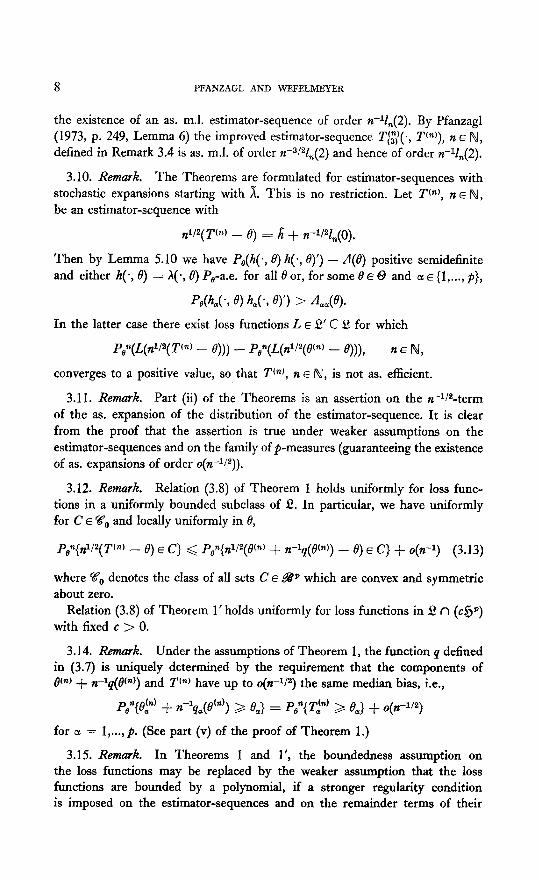
the existence of an as. m.1. estimator-sequence of order n-V,(2). By Pfanzagl (1973, p. 249, Lemma 6) the improved estimator-sequence T$(., T(n)), n E N, defined in Remark 3.4 is as. m.1. of order n-3/Z&(2) and hence of order n-V,(2).
3.10. Remmk. The Theorems are formulated for estimator-sequences with stochastic expansions starting with x. This is no restriction. Let T(e), it E N, be an estimator-sequence with
d&r(“) - e) = II + n-vzn(o)~
Then by Lemma 5.10 we have P,(h(., 0) A(,, 0)‘) - A(0) positive semidefinite and either A(*, 8) = A(., 6) PO- a.e. for all0or,forsome8EO and a~{1 ,..., $1,
pdkk, 8) kc, w b 4,(e).
In the latter case there exist loss functions L E 2 C S for which
P,n(L(dyr(n) - 8))) - PoyL(dqe(~) - e))), flEN/,
converges to a positive value, so that Fn), n E N, is not as. efficient.
3.11. Remark. Part (ii) of the Theorems is an assertion on the n-l12-term of the as. expansion of the distribution of the estimator-sequence. It is clear from the proof that the assertion is true under weaker assumptions on the estimator-sequences and on the family of p-measures (guaranteeing the existence of as. expansions of order ~(n-~‘“)).
3.12. Remark. Relation (3.8) of Th eorem 1 holds uniformly for loss func- tions in a uniformly bounded subclass of X!. In particular, we have uniformly for C E W,, and locally uniformly in 8,
~~yd/y~fn) - e) E cl < pgqaye(n) + +(ey - e) E cl + o(q (3.13)
where ‘ips denotes the class of all sets C E %?p which are convex and symmetric about zero.
Relation (3.8) of Theorem 1’ holds uniformly for loss functions in 2 n (c$jp) with fixed c > 0.
3.14. Remark. Under the assumptions of Theorem 1, the function 4 defined in (3.7) is uniquely determined by the requirement that the components of W + n-l&W) and Z’cn) have up to o(n-l/s) the same median bias, i.e.,
p,yep) + n-lqa(e(=J) 2 e,2 = 2yf~f) 3 e,) + o(lt-1’2)
for CL = l,...,p. (See part (v) of the proof of Theorem 1.)
3.15. Remark. In Theorems 1 and l’, the boundedness assumption on the loss functions may be replaced by the weaker assumption that the loss functions are bounded by a polynomial, if a stronger regularity condition is imposed on the estimator-sequences and on the remainder terms of their
MAXIMUM LIKELIHOOD ESTIMATOR 9
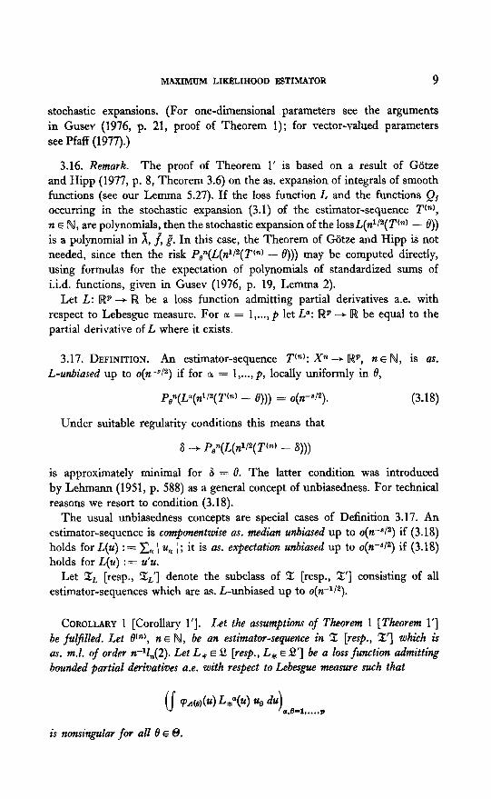
stochastic expansions. (For one-dimensional parameters see the arguments in Gusev (1976, p. 21, proof of Theorem 1); for vector-valued parameters see Pfaff (1977))
3.16. Remark. The proof of Theorem 1’ is based on a result of G&e and Hipp (1977, p. 8, Theorem 3.6) on the as. expansion of integrals of smooth functions (see our Lemma 5.27). If the loss function L and the functions Q, occurring in the stochastic expansion (3.1) of the estimator-sequence WI, n E N, are polynomials, then the stochastic expansion of the los~L(d~~(Z’~~) - 0)) is a polynomial in x, f, g”. In this case, the Theorem of G&e and Hipp is not needed, since then the risk PO”(L(n112(T (n) - 0))) may be computed directly, using formulas for the expectation of polynomials of standardized sums of i.i.d. functions, given in Gusev (1976, p. 19, Lemma 2).
Let L: iJ!p -+ [w be a loss function admitting partial derivatives a.e. with respect to Lebesgue measure. For OL = l,..., p let La: W + R be equal to the partial derivative of L where it exists.
3.17. DEFINITION. An estimator-sequence Ten): Xn + W, n E N, is us. L-unbiased up to o(n-“j2) if for cy = I,..., p, locally uniformly in e,
P&L~(nlyT(n) - e))) = o(n-812).
Under suitable regularity conditions this means that
(3.18)
6 -+ Pen(L(nyT(n) - 6)))
is approximately minimal for S = 0. The latter condition was introduced by Lehmann (1951, p. 588) as a general concept of unbiasedness. For technical reasons we resort to condition (3.18).
The usual unbiasedness concepts are special cases of Definition 3.17. An estimator-sequence is componentwise as. median unbiased up to o(n-“1”) if (3.18) holds for L(u) : = Cu 1 u, 1; it is as. expectation unbiased up to o(n-“j2) if (3.18) holds for L(u) := u’u.
Let Zt [resp., Z,‘] denote the subclass of Z [resp., S’] consisting of all estimator-sequences which are as. L-unbiased up to o(n-lj2).
COROLLARY 1 [Corollary 1’1. Let the assumptions of Theorem 1 [Theorem 1’1 be fulfilled. Let tY*), n E N, be an estimator-sequence in 2 [resp., 211 which is as. m.1. of order n-Y,(2). Let L* E (! [resp., L, E !Z] be a loss function admitting bounded partial derivatives a.e. with respect to Lebesgue measure such that
is nonsingular fm all e E 8.
10 PFANZAGL AND WJZFELMEYER
Then there exists q*: 0 3 E4’ such that tke estimator-sequence W + rlq*(W), n E N, is third-order eflcient in Z,., [resp., X;J. More precisely: O(@ + rlq*(@“)),
n E N, is in ZL, [resp., %;,I, and for every estimator-sequence T(“), n E IV, in
2,* [vesp., irt,] and every loss function L E l! [resp,, L E 9’1 we have locally uniformly in 6
P,fi(L(?W(P’ + n-lq*(W) - e))) < P&L(@(T(n) - e))) + o(n-‘).
3.19. Remark. Under the assumptions of Corollary 1 the correction for componentwise as. median unbiasedness up to ~(n-r/~) is
9a* : = AfJ4&?,%8 + ib%.vs)
- 4iwdtw~ast8LB.%* + -k&3.,.*)- (3.20)
For one-dimensional parameters the result for median unbiased estimators was given by Pfanzagl (1975, p. 37, Theorem 7).
3.21. Remark. Under the stronger regularity conditions mentioned in Remark 3.15 we obtain the result of the Corollaries for estimators which are as, expectation unbiased up to ~(n-l/~). The corresponding correction for the m.1. estimator is
4a* : = &4&&3,v,G + &3ms)* (3.22)
3.23. Remark. The risks of as. efficient estimator-sequences having the same bias up to ~(n-l/~) differ in the n-l-term only. If we compare such estimator- sequences on the basis of their risks, we find that the conclusion depends on the underlying loss function even if it is symmetric. Related to this is the fact that deficiency, too, depends on the particular loss function. In contrast to this, the optimality of the (corrected) m.1. estimator expressed in Corollaries 1, 1’ holds simultaneously for all loss functions in L! [resp., 2’1.
For multinomial families with one-dimensional parameter, C. R. Rao (1963, p. 205) states (without proof) the optimality with respect to the quadratic loss function of the m.1. estimator corrected for expectation unbiasedness in the class of estimators which are solutions of an estimating equation; Ponnapalli (1976, p. 44, Lemma 2) computes the relative deficiencies of (uncorrected) minimum discrepancy estimators on the basis of their variances and obtains (p. 47, Corollary) a condition under which the ml. estimator is optimal among such estimators.
For multinomial families with vector parameter, Robertson (1972, p. 140, Theorem 1) proves that the ml. estimator is optimal in the class of minimum discrepancy estimators in the sense that its covariance matrix differs from that of a minimum discrepancy estimator by a term np2c2N which depends on the minimum discrepancy estimator through c only. However, this is a reasonable optimum property only if the matrix N is positive semidefinite, a property not claimed by the author but hopefully true.
MAXIMUM LIKELIHOOD ESTIMATOR 11
For one-dimensional curved exponential families and the class of (corrected) locally stable estimators (cf. the bibliographical note following our Theorems), the optimality of the m.1. estimator corrected for expectation unbiasedness is obtained by J. K. Ghosh and K. Subramanyam (1974, p. 336, Theorem l(ii)) for the truncated quadratic loss function and by Efron (1975, p. 1209, Remark 2) for the ordinary quadratic loss function.
For multidimensional curved exponential families, J. K. Ghosh and K. Subramanyam (1974, p. 346, Remark (1)) state that the difference between the +-terms of the as. expansions of the covariance matrices of an arbitrary locally stable estimator and the m.1. estimator is positive semidefinite. As a consequence, the m.1. estimator is optimal if the comparison is based on the “generalized variance” (i.e. the determinant of the covariance matrix) of the estimator. This is proved in Ponnapalli (1977, Theorem 4.4). In the one- dimensional case, the comparison of generalized variances reduces to comparing risks with respect to the quadratic loss function. In the multidimensional case, however, the operational significance of this concept remains to be demonstrated.
3.24. Remark. It is easily seen from relation (6.19) and the ensuing dis- cussion that Theorems 1 and 1’ admit the following generalizations.
Let the assumptions of Theorem 1 [Theorem l’] be fulfilled. Let Ten), n E FY, be an estimator-sequence in Z [resp., 2’1 with the additional property that for some 4: @ -+ [WP and all 8 E @
(3.25)
where Qr denotes the n-l12-term of its stochastic expansion (3.1). (Notice that ~(8) = 0 if the estimator-sequence To’), n E N, is as. ml. of order n-l&(2).)
Then the estimator-sequence Ten) + n-l(q( T(“)) - p( T(“))), a E N, has the optimum property expressed in part (iii) of Theorem 1 [Theorem 1’1 for the corrected m.1. estimator-sequence Btn) + n-$(0(“)), n E N.
Moreover, the estimator-sequence Ten) + n-l(q*( T(“)) - p( Ttn))), n E NJ, is as. &-unbiased up to o(n-lj2) and optimal in the sense of Corollary 1 [Corollary 1’1.
We remark that (3.25) implies
T(n) = e(n) + n-lij + n-3i31n(2), (3.26)
hence $%) - .-qj(p)) = e(n) + n-34,p).
This is an immediate consequence of Lemma 5.12 on the “canonical representa- tion” of the stochastic expansion of an estimator-sequence.
The above result is of interest because many estimators related to Bayesian theory fulfill (3.25) and therefore have the optimum properties stated in Theorems 1 and 1’ and in Corollaries I and 1’ for the m.1. estimator. We shall
12 PFANZAGL AND WEFELMEYER
demonstrate this for the case of a one-dimensional parameter, where the necessary stochastic expansions are available in literature.
(i) Let d{;:, n E N, be a sequence of generalized Bayes estimators with respect to a homogeneous loss function of degree a and a prior measure with Lebesgue density W. Then by Gusev (1975, p. 484, Theorem 4; see also Strasser (1977b), p. 32, Theorem 4)
t# = 6’“’ + n-$q,!J+r) - &L;E2Llll(U + 1))
+ n-3’“4&(2).
(ii) For i = 2 resp., i = 3 let t{r;, n E N, be a sequence of modes (resp., medians) of the posterior density. Then by Gusev (1975, p. 476, Theorem 1) [resp., Strasser (1977b, p. 20, Theorem 2)]
t$ = d”’ + n-‘L;.11(7+) + n-“‘“l,(2), i = 2, 3.
The particular form of the stochastic expansions of the three estimator- sequences t#, n E N, discussed in (i) and (ii) has a further consequence: One can choose the prior density r such that these estimator-sequences are as. equivalent to any given estimator-sequence To’), n E N, with property (3.25) in the sense that
t($’ = T’“’ + n-3’3142). (3.27)
Hence, using one of the estimator-sequences t{$, n E N, an as. complete class of order o@z-~) can also be obtained by varying the prior density (instead of using varying correction terms). The prior density can in particular be chosen such that the pertinent estimator-sequence t[$, n E N, is as. equivalent in the sense of (3.27) to the m.1. estimator-sequence P), n E N, or such that t$, n E N, is as. median unbiased up to o(n-l12); see Strasser (1977b, p. 34, Theorem 5, and p. 24, Example 1).
The stochastic expansions given in (i) and (ii) yield immediately the following result: For each of the three estimator-sequences t{F/, n E N, there exists a locally bounded ci: 0 -+ R such that locally uniformly in 0
P@n{l t$ - e(n) 1 > c.(e) n-l} = o(~z-~). t I
(By (3.26) this holds, in fact, for all estimator-sequences with property (3.25).) For the Bayes estimator this result is proved in Strasser (1977a, p. 364, Theorem 4).
3.28. Remark. Define
MAXIMUM LIKELIHOOD ESTIMATOR 13
Then Corollaries 1 and 1’ remain true if in the definitions (3.20) and (3.22) of q* the symbols A, LB,r,B, LBsva are replaced by b, &Y,s, &YB, respectively. This modification is useful if the integrals L,,, , LB,vs are difficult to compute. For the proof, observe that this modification does not affect the stochastic expansion of P) + &~*(W), tl E N, up to terms of order n-V,(2). Hence by (6.19) it leaves the risks unchanged up to o(n-I).
Similarly, the improvement procedure defined in Remark 3.4 can be modified, replacing x, by &,es.
3.29. Remmk. The above results may also be applied to the problem of estimating a subvector, say 8, , of the unknown parameter ti = (0, , 6,). Let e(n) = (et;;, 8;;;): n E N, be as. m.1. of order n-V,(2). Then, under appropriate regularity conditions, e{;f:, 71 E N, is optimal in the sense of Theorems 1 and 1’ and Corollaries 1 and 1’ in the class of all estimator-sequences of 6, . (This follows easily from the fact that each estimator-sequence Tt,“, n E N, of 6, can be complemented to an estimator of the whole parameter (6, , es), e.g.
to G’TA hh w to which the theorems and corollaries apply.)
4. REGULARITY CONDITIONS
In this section we collect the regularity conditions which are needed for the proofs.
(i) Pe 1 J&‘, 0 E 0, are mutually absolutely continuous.
(ii) L; = 0 on 0.
(iii) L is positive definite on 0.
Conditions M, , L, , D refer to a function f: X x 0 + I&
CONDITION Ms . For every BE 0 there exists a neighborhood U, of B such that
SUP em(-, ew < 00. B’.B’EU.g
CONDITION L, . There exists a function k: X x 0 -+ Iw and for every 8 E 0 there exists a neighborhood U, of t9 such that
(a) jf(~, e') -f(x, em)1 < jj 8’ - 8” 11 k(x, e) for x E X and e’, 8" E u, .
(b) k fulfills Condition M, .
CONDITION D. For f(*, T)(#, 1 d)/(&‘@ I -QI) the order of integration with respect to Pe [ .& and differentiation with respect to T is interchangeable at 7 = 8 for every e E 0.
14 PFANZAGL AND WEFELMEYER
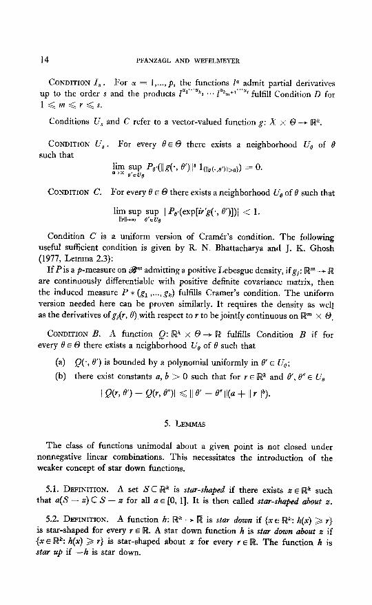
CONDITION I,. For cz = 1 ,...,p, the functions P admit partial derivatives up to the order s and the products 1”‘“‘““l ... loLkm+l”‘“’ fulfill Condition D for l<m<r<s.
Conditions U, and C refer to a vector-valued function g: X x 0 ---f W.
CONDITION U,. For every d E 0 there exists a neighborhood U, of 6 such that
lim SUP p&llg(-, e'>ll" l~b(.,~w>~)) = 0. a+m B'Eug
CONDITION C. For every 8 E 0 there exists a neighborhood U, of 8 such that
Condition C is a uniform version of Cram&s condition. The following useful sufficient condition is given by R. N. Bhattacharya and J. K. Ghosh (1977, Lemma 2.3):
If P is a p-measure on W” admitting a positive Lebesgue density, ifgj: [w” -+ [w are continuously differentiable with positive definite covariance matrix, then the induced measure P c (gI ,..., gk) fulfills Cramer’s condition. The uniform version needed here can be proven similarly. It requires the density as well as the derivatives of g,(r, 0) ,with respect to r to be jointly continuous on [w” x 0.
CONDITION B. A function Q: 88” x 0 x + 88 fulfills Condition B if for every 0 E 0 there exists a neighborhood lJ, of 0 such that
(a) Q(., 0’) is bounded by a polynomial uniformly in 8’ E Ue;
(b) there exist constants a, b > 0 such that for Y E W and 0’, 0” E U,
I Q@, 8’) - Q(c @‘)I < II 0’ - 8” II@ + II r II”>.
5. LEMMAS
The class of functions unimodal about a given point is not closed under nonnegative linear combinations. This necessitates the introduction of the weaker concept of star down functions.
5.1. DEFINITION. A set SC tRk is star-shaped if there exists z E I?%‘% such that a(S - z) C S - z for all a E [0, 11. It is then called stat-shaped about z.
5.2. DEFINITION. A function h: Iwk + R is star down if (x E W: h(x) > Y} is star-shaped for every Y E Iw. A star down function h is star down about x if (x E W: h(x) 3 r> is star-shaped about x for every T E Iw. The function h is star up if -h is star down.
MAXIMUM LIKELIHOOD ESTIMATOR 15
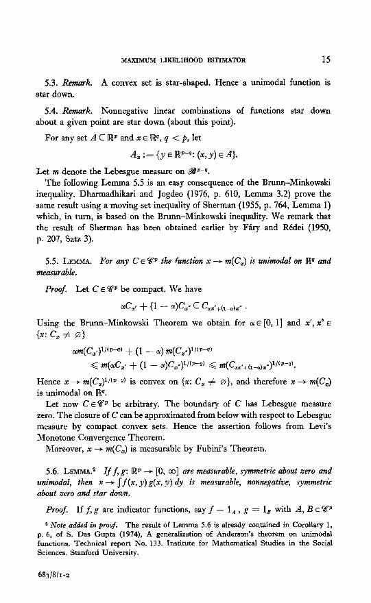
5.3. Remark. A convex set is star-shaped. Hence a unimodal function is star down.
5.4. Remrk. Nonnegative linear combinations of functions star down about a given point are star down (about this point).
For any set A C Iw’ and x E Iwq, 4 < p, let
A, := {y E W-Q: (x, y) E A).
Let m denote the Lebesgue measure on BP-Q. The following Lemma 5.5 is an easy consequence of the Brunn-Minkowski
inequality. Dharmadhikari and Jogdeo (1976, p. 610, Lemma 3.2) prove the same result using a moving set inequality of Sherman (1955, p. 764, Lemma 1) which, in turn, is based on the Brunn-Minkowski inequality. We remark that the result of Sherman has been obtained earlier by FBry and RCdei (1950, p. 207, Satz 3).
5.5. LEMMA. For any C E 23 the function x + m(C,) is unimodal on IW’J and measurable.
Proof. Let C E %P be compact. We have
&I!~ + (1 - 4G” c &!‘+(1-a)z” *
Using the Brunn-Minkowski Theorem we obtain for OL E [0, I] and x’, x” E lx: c, # a>
Olm(Ca~)l/(P-q) + (1 - a) m(C3ce)1/(P-q)
< rn(&,, + (1 - 0L)C,z~)11(P--9) < m(Carx,+(l-~~o”)ll(P-q).
Hence x + m(C.#I(p-‘J) is convex on (x: C, # ia>, and therefore x -+ m(C,) is unimodal on Iwq.
Let now C E%‘D be arbitrary. The boundary of C has Lebesgue measure zero. The closure of C can be approximated from below with respect to Lebesgue measure by compact convex sets. Hence the assertion follows from Levi’s Monotone Convergence Theorem.
Moreover, x -+ m(C,) is measurable by Fubini’s Theorem.
5.6. LEMMA.~ If f, g: [WV + [0, a] are measurable, symmetric about zero and unimodal, then x --+ sf (x, y) g(x, y) dy is measurable, nonnegative, symmetric about zero and star down.
Proof. If f, g are indicator functions, say f = lA , g = Is with A, B E W
2 Note added in proof. The result of Lemma 5.6 is already contained in Corollary 1, p. 6, of S. Das Gupta (1974), A generalization of Anderson’s theorem on unimodal functions. Technical report IVo. 133. Institute for Mathematical Studies in the Social Sciences. Stanford University.
683/8/r-2
I6 PFANZAGL AND WEFELMEYER
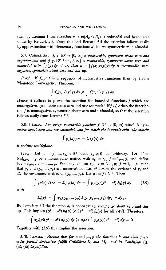
then by Lemma 1 the function x -+ m(A, n B,) is unimodal and hence star down by Remark 5.3. From this and Remark 5.4 the assertion follows easily by approximation with elementary functions which are symmetric and unimodal.
5.7. COROLLARY. Iffy Iwp --f [0, co] is measurable, symmetric about zero and neg-unimodal and if g: !W--q --f [0, co] is measurable, symmetric about zero and z&modal with sg(y) dy < 00, then x + sf(x, y) g(y) dr is measurable, non- negative, symmetric about zero and star up.
Proof. If fnf f is a sequence of nonnegative functions then by Levi’s Monotone Convergence Theorem,
j f&G Y) g(y) dY f j fc? Y> E(Y) dY*
Hence it suffices to prove the assertion for bounded functions f which are nonnegative, symmetric about zero and neg-unimodal. Iff < c then the function c - f is nonnegative, symmetric about zero and unimodal, so that the assertion follows easily from Lemma 5.6.
5.8. LEMMA. For every measurable function f: RP + [0, w) which is sym- metric about zero and neg-unimodal, and for which the integrals exist, the matrix
I E&>(xx’ - 2) f(x) dx
is positive semide$nite.
Proof. Let c = (ci ,..., cP)’ E 5P with c, # 0 be arbitrary. Let C =
(Cdi.*=l*....P be a nonsingular matrix with crj = cj , j = l,...,p, and define yi := cijxj , i = I,..., p. We may choose cii , i = 2 ,..., p; j = l,..., p, such that yr and (ys ,..., y,) are uncorrelated. Let u2 denote the variance of yr and 2s the covariance matrix of (ys ,..., yP). Let h := f 0 C-l. Then
s ~(4 c’W - 2:) cf(x) dx = j P~~(Y)(Y’ - ~“1 MY) 4 (5.9)
with
ho(y) := j F,Y&Y~ j..-, YA hb, y2 I..., ~9) 4, **- dyp .
By Corollary 5.7 the function h, is nonnegative, symmetric about zero and star up. This implies (y2 - u”) h,(y) > ( y2 - 9) h,,(u) for all y E U&‘. Therefore,
j R,~Y)(Y” - ~‘1 ho(~) dr 2 M4 j VQ(Y)(Y~ - 0”) dr = 0.
Together with (5.9) this implies the assertion.
5.10. LEMMA. Assume that for a = l,..., p the functions P and their first- order part&al akrivatives @I$11 C&itSms L, and M, , and let Conditions (i), (ii), (iii) be fulJlled.
MAXIMUM LIKRLIHOOD ESTIMATOR 17
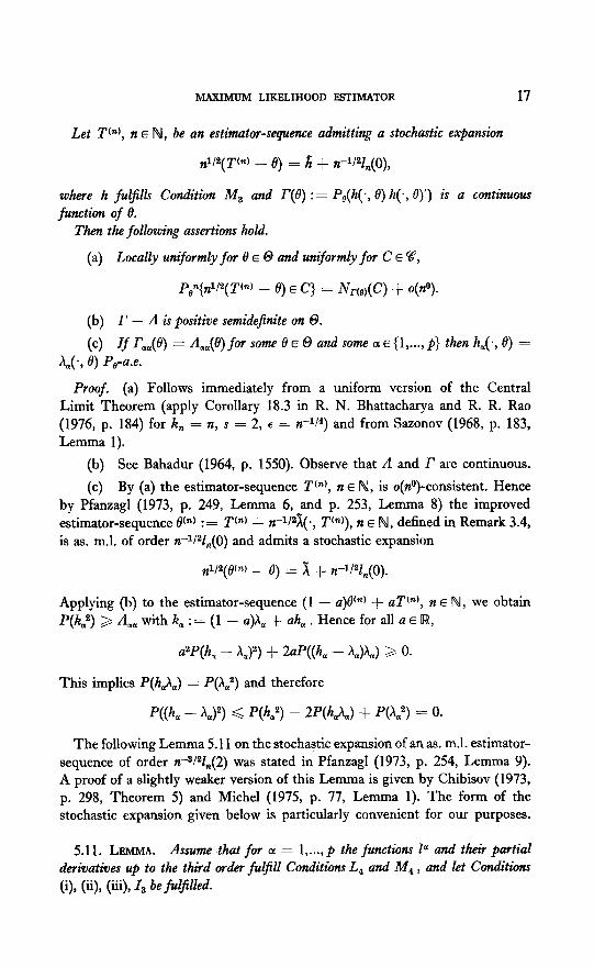
Let T(n), n E N, be an estimator-sequence admitting a stochastic expansion
@(T(n) - 6) = iE + n-lj2Zn(0),
where h fuZ&!s Condition M3 and r(e) := P,(h(., 0) h(., 0)‘) is a continuous fun&m of e.
Then the following assertions hold.
(a) Locally uniforms for tl E 0 and uniformly for C E V,
pe”(ni/2(T(n) - e) E c} = N,(,)(c) + O(?Z').
(b) r - A is positive semidejinite on 8.
(c) rf r,,(e) = f3,,(e) for ~0ttte e E 0 and SOL oL E (I,..., p> then h,(., e) = A,(-, e) P,-a.e.
Proof. (a) Follows immediately from a uniform version of the Central Limit Theorem (apply Corollary 183 in R. N. Bhattacharya and R. R. Rao (1976, p. 184) for R, = n, s = 2, E = n-1j4) and from Sazonov (1968, p. 183, Lemma 1).
(b) See Bahadur (1964, p. 1550). Ob serve that A and r are continuous.
(c) By (a) the estimator-sequence T(“), n E N, is o(nO)-consistent. Hence by Pfanzagl (1973, p. 249, Lemma 6, and p. 253, Lemma 8) the improved estimator-sequence W := T(“) + n-1/2X(., T(n)), n E N, defined in Remark 3.4, is as. m.1. of order n-1/2Zn(0) and admits a stochastic expansion
dP(iP) - e) = X + n-l121,(0).
Applying (b) to the estimator-sequence (1 - a)W + aTcn), n E N, we obtain P(K,2) > rl,, with K, := (1 - a)& + ah, . Hence for all a E Iw,
a2P(h, - Qz) + 2aP((h, - h,)h,) > 0.
This implies P(h,h,) = P(ha2) and therefore
P((h, - hJ2) < P(ha2) - 2P(h,h,) + P(l\.“) = 0.
The following Lemma 5.11 on the stochastic expansion of an as. m.1. estimator- sequence of order n-“/“Z,(2) was stated in Pfanzagl (1973, p. 254, Lemma 9). A proof of a slightly weaker version of this Lemma is given by Chibisov (1973, p. 298, Theorem 5) and Michel (1975, p. 77, Lemma 1). The form of the stochastic expansion given below is particularly convenient for our purposes.
5.11. LEMMA. Assume that for a = l,..., p the functions Ia and their partial derivatives up to the third order fulfill Conditions L, and M4 , and let Conditions (i), (ii), (iii), 1, be fuZj%ed.
18 PFANZAGL AND WEFELMEYER
(a) If W, n E k.4, is as. m.1. of order n-3/21,(2) then
nlla(p - e) = x + n--1/2[Tia(Xa 1 A) - &&P(P)]
+ n-'[XJJ.J~P(P') + gP(Pr))
- &l&iv 1 A) P@)
+ u&T I m6 I 4 + bu3(~8 I 41
+ n-3’21,(2).
(b) If W, n E N, is as. m.1. of order n-Y,,(2) then
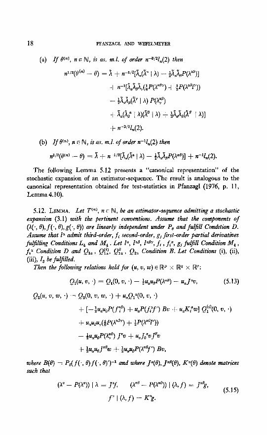
nii2(e(n) - e) = X + n-1/2[1&N 1 h) - &X,X,P(X~e)] + n-V,(2).
The following Lemma 5.12 presents a “canonical representation” of the stochastic expansion of an estimator-sequence. The result is analogous to the canonical representation obtained for test-statistics in Pfanzagl (1976, p. 11, Lemma 4.10).
5.12. LEMMA. Let T(“), n E N, be an estimator-sequence admitting a stochastic expansion (3.1) with the pertinent conventions. Assume that the components of
oh af c, 8, d., 4) are linearly independent under Pe and fulfill Cond&n D. Assume that 10 admit third-order, fi second-order, gj first-order partial derivatives fulfilling Conditions L, and Me . Let la, l0e, W’, fi , fia, gj fu@ll Condition Me , faoi Condition D and QIN , Qc, Q& , Qza. Condition B. Let Conditions (i), (ii), (iii), I3 be fuljlled.
Then the following relations hold for (u, v, w) E LV x FP x IF!':
Qdu, v, .) = Qdo, v, *) - Qu,ueP(h”s) + u,J”v, (5.13)
Q204 v, w, -1 = Q2(0, vu, w, +> + u,QiV, v, *I
+ [-&w,P(f5B) + Q(fe'f') Bv + u,Gwl Q:'(O, 0, a)
+ u,upu,(QP(X@‘) + $P(A”V))
- &ueP(X;*) J”v + ua Jo% Jew
+ &,ueJ”cw + &ueP(X=ef ‘) Bv,
where B(0) = P,( f (., 0) f (., 0)‘))l and where p(O), J”@(O), Ka(0) denote matrices such that
(A” - P(Y)) ] x = J% vs - m9 I (h f) = J.% (5.15)
f" I (kf) = q?.
MAXIMUM LIKELIHOOD ESTIMATOR 19
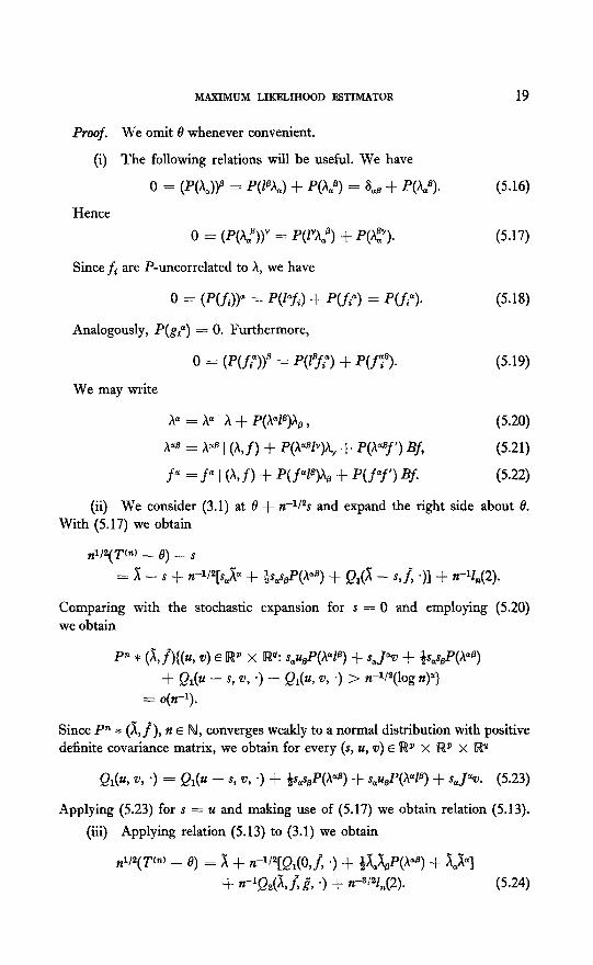
Proof. We omit 8 whenever convenient.
(i) The following relations will be useful. We have
0 = (P(A# = P(Z6i,) + P&q = 6, + P(x,e). (5.16)
Hence
0 = (P(A,s))’ = P(ZYh,B) + P(A?). (5.17)
Since fi are P-uncorrelated to X, we have
0 = (P(f# = P(Z”f) + P(fp) = P(fiy. (5.18)
Analogously, P&a) = 0. Furthermore,
0 = (P(f$y = P(Z8f,) + P(fi”). (5.19)
We may write
Xa = A” 1 h + P(xqA, , (5.20)
hug = P 1 (A, f) + P(A”V)h, + P(h”‘3f’) Bf, (5.21)
f” = f” I (hf) + P(f”Z”)b + P(f”f ‘) Bf. (5.22)
(ii) We consider (3.1) at 0 + n-14 and expand the right side about 0.
With (5.17) we obtain
&2(p) - lg) - s
= x - s + n-l/2[s,% + &.s~P(A”~) + Q&i - s,J, .)] + d,(2).
Comparing with the stochastic expansion for s = 0 and employing (5.20)
we obtain
P” * (X,J){(z4, v) E R” x w: sausP(A”ZB) + s, J”e) + +&P(A=B)
+ Ql(u - s, v, -) - Ql(u, v, .) > d2(log up}
= o(n-1).
Since Pn * (X, j), n E N, converges weakly to a normal distribution with positive definite covariance matrix, we obtain for every (s, u, v) E IwP x IR” X R’J
Q1(u, v, -) = Ql(u - s, v, -) + &as8P(X=f?) + sau6P(A=Z8) + s.J”v. (5.23)
Applying (5.23) f or s = u and making use of (5.17) we obtain relation (5.13).
(iii) Applying relation (5.13) to (3.1) we obtain
@(T(n) - 0) = x + n-‘l*[Ql(O,f, .) + B&&$‘(~~6) + kxal + n-lQ&, i g’, .) + r3W,(2). (5.24)
20 PFANZAGL AND WEFELMEYER
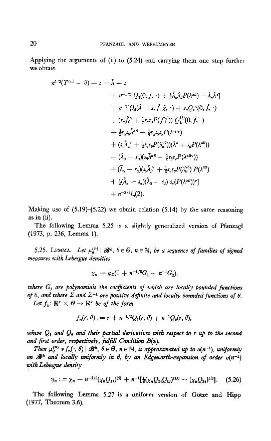
Applying the arguments of (ii) to (5.24) and carrying them one step further we obtain
n1/2(T’“) - 0) - s = i - s
Making use of (5.19)-(5.22) we obtain relation (5.14) by the same reasoning as in (ii).
The following Lemma 5.25 is a slightly generalized version of Pfanzagl (1973, p. 236, Lemma 1).
5.25. LEMMA. Let pr’ 1 Wk, 0 E 0, n E N, be a sequence of families of signed measures with Lebesgue densities
xn = v.r(l + c~/~G, + n-lG,),
where Gi are polynomials the coej&-nts of which are locally bounded functions of 8, and where Z and .I? are positive deJnite and locally bounded functions of 8.
Let fn: Rk x 0 -+ [Wk be of the form
fn(y, q := r + +‘2Q&, q + n-lQ&, q,
where QI and Q2 and theik partial derivatives with respect to T up to the second and jirst order, respectively, filfZ1 Condt’tzim B(a).
Then &‘) * f,,(., 0) 1 ak, B E 8, n E N, is approximated up to o(n-l), un;formly on SF and locally uniformly in B, by an Edgeworth-expans&m of order o(n-‘) with Lebesgue density
%I := xn - n-1/2(,ynQli)(“) + n-l[Q(x,QliQlr)(ij) - (xnlQa#)]. (5.26)
The following Lemma 5.27 is a uniform version of Gijtze and Hipp (1977, Theorem 3.6).
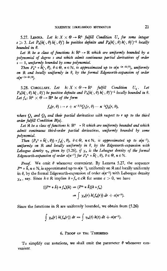
MAXIMUM LIKELIHOOD ESTIMATOR 21
5.27. LEMMA. Let h: X x 8 + Rk fulfill Condition U, for some integer s >, 3. Let Pe(h(., 0) h(., 19)‘) be positiwe definite and Pe(h(*, 6) h(*, e)‘)-l locully
bounded in 8. Let 53 be a class of functions k: lRk -+ R which are uniformly bounded by a
polynomial of degree s and which admit continuous partial derivatives of order s - 1, uniformly bounded by some polynomial.
Then Pen * h(., e), BE 0, n E N, is approximated up to o(n-(8-2)/2), uniformly on R and locally uniformly in 0, by the formal Edgeworth-expansion of order o(n-(S-2)/2 )*
5.28. COROLLARY. Let h: X x 0 + Rk fu&ll Condition U, . Let
Pi&(., 0) ht., ej’) b e P osi ive definite and Pe(h(., 0) h(., O)‘)-1 locally bounded in 0. t Let fn: Wk x 0 -+ lRk be of the form
fn(r, 0) :== r + n-1’2Q1(r, 0) + n-lQ,(r, 4,
where QI and Q2 and their partial derivatives with respect to Y up to the third order fulfill Condition B(a).
Let 53 be a class of functions k: Rk + R which are uniformly bounded and which admit continuous third-order partial derivatives, uniformly bounded by some polynomial.
Then (P,” * h(., e)) * fn(., e), e f 0, 12 E N, is approximated up to o(n-l), uniformly on R and locally uniformly in 8, by the Edgeworth-expansion with
Lebesgue density r],, given by (5.26), if xn is the Lebesgue density of the formal Edgeworth-expansion of order o(n-l) for POn * h(., e), 0 E 0, n E N.
Proof. We omit t9 whenever convenient. By Lemma 5.27, the sequence Pn or f;, n E IV, is approximated up to o(n-l), uniformly on R and locally uniformly in 0, by the formal Edgeworth-expansion of order o(n-I) with Lebesgue density
Xn 3 say, Since k E R implies k 0 fn E CR for some c > 0, we have
W’” * i) *fn>(h) = (P” * h)(k of,,)
= I x&) k(f,@)) dr + o(n-7.
Since the functions in 33 are uniformly bounded, we obtain from (5.26)
s x,,(r) k(f&)) dr = s G) k(t) dt + o(n-‘).
6. PROOF OF THE THEOREMS
To simplify our notations, we shall omit the parameter 8 whenever con- venient .
22 PFANZAGL AND WEFELMEYER
The proof of Theorem 2 is nearly identical to the proof of Theorem 1. The necessary modifications are indicated in square brackets.
Let fi denote a class of functions K: IIP x Iwq x Rr -+ Iw which are uniformly bounded and which admit continuous third order partial derivatives, uniformly bounded by some polynomial.
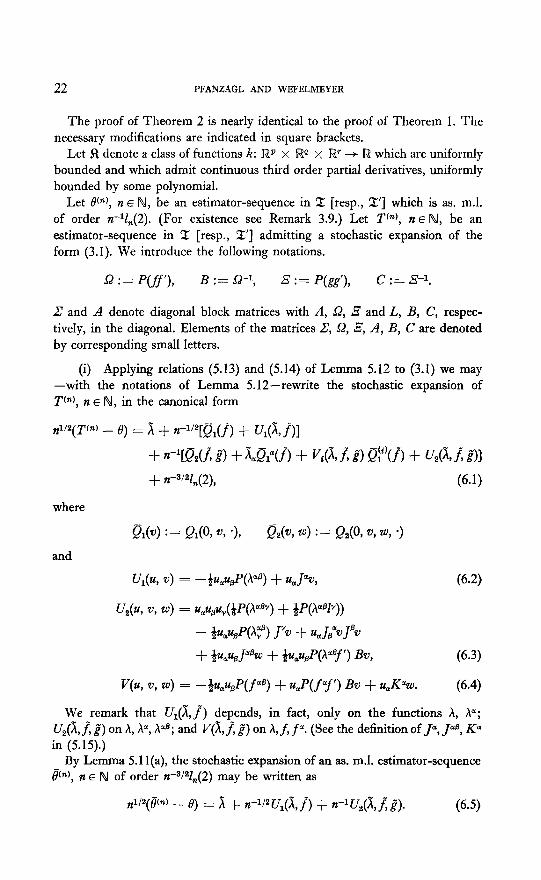
Let P), II E N, be an estimator-sequence in 2 [resp., 2’1 which is as. m.1. of order n-V,(2). (For existence see Remark 3.9.) Let T(“), n E N, be an estimator-sequence in Z [resp., 2’1 admitting a stochastic expansion of the form (3.1). We introduce the following notations.
sz := P(ff’), B := 52-l, B := Pk’>, c := E-1.
Z and A denote diagonal block matrices with A, Q, % and L, B, C, respec- tively, in the diagonal. Elements of the matrices C, 52, s, A, B, C are denoted by corresponding small letters.
(i) Applying relations (5.13) and (5.14) of Lemma 5.12 to (3.1) we may -with the notations of Lemma 5.12-rewrite the stochastic expansion of T(n), n E N, in the canonical form
.1’2(T’“’ - e> = x + n-1’2[(Jl(f) + U,(X,f)]
+ qQ2(J 2) + k&cJ> + K(JLL 8 lew> + u26i.i a1
+ n-W,(2), (6-l)
where
&l(W) := MO, w> .>, Q2h 4 := &2(O,w, *, -1
and
Ul(U, w) = -;ulyuBP(w) + u,Juw, 6.2)
U2(u, w, w) = u,u,,g&P(~“6y) + pyh”W)
- &u,~(h”;B) J’w + u, Ja”wJBv
+ +uau6J”Bw + &q@(Pf ‘> Bw, (6.3)
V(u, w, w) = -&usP(f”~) + uaP(f”f ‘) Be, + u,Kaw. (6.4)
We remark that U,(x,j) d p d e en s, in fact, only on the functions h, ha; U,(i, f, g”) on X, ha, P; and V(i,f, g”) on /\, f, f”. (See the definition of J”, J”s, Ku in (5.15).)
By Lemma 5.1 l(a), the stochastic expansion of an as. m.1. estimator-sequence 8(m), n E N of order n-3/2&(2) may be written as
n l 2 -(?I) - 8) = x + n-fWl(X,fl) + n-‘U2(X,J,g”). J (B (6.5)
MAXIMUM LIKRLIHOOD ESTIMATOR 23
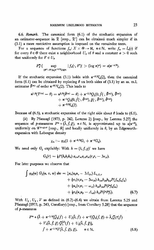
6.6. Remark. The canonical form (6.1) of the stochastic expansion of an estimator-sequence in 2 [resp., T] can be obtained much simpler if in (3.1) a more restrictive assumption is imposed on the remainder term.
For a sequence of functions fn: X x 0 --f R, n E N, write fn = l,(s) if for every ~9 E 0 there exist a neighborhood U, of 0 and a constant a > 0 such that uniformly for 8’ E U,
m ,,8”-B,,,<n-‘,aIogn I fn(., 01 > P% WI = oV2)* sup
If the stochastic expansion (3.1) holds with n-3/2&(2), then the canonical form (6.1) can be obtained by replacing 0 on both sides of (3.1) by an as. ml. estimator @) of order n-“l”Z,(2). This leads to
&“( T(n) - e) = dyB(n) - e) + n-l/2Q1(o,J(., 8y, 8(n))
+ n-lQ,(O,fl(*, 8cn’), g’(., @)), @‘) + n-3/31,(2).
Because of (6.5), a stochastic expansion of the right side about 6 leads to (6.1).
(ii) By Pfanzagl (1973, p. 242, Lemma 2) [resp., by Lemma 5.271 the sequence of p-measures Pn * (A, J, j), n E IV, is approximated up to o(n-l), uniformly on %p+q+F [resp., R] and locally uniformly in 8, by an Edgeworth- expansion with Lebesgue density
X7% := &l + .-1/2G, + +G,).
We need only Gi explicitly: With h = (A, f , g)’ we have
G(r) = BP(~Jh) aimrmaj4r8~t - 3~~).
For later purposes we observe that
1 n&4 W, 0, 4 dw = BUwv - 3&J Lx.~.v
+ &Jih% - 3w37c) Lrl+nbk?S(fmf,f9) + BG+~~ - 4 bh7Jwfkicfm) + +4(w, - 4,) @y~“~@fj). (6.7)
With Vi , U, , V as defined in (6.2)-(6.4) we obtain from Lemma 5.25 and Pfanzagl (1973, p. 243, Corollary) [resp., from Corollary 5.281 that the sequence of p-measures
24 PFANZAGL AND WEFELMEYER
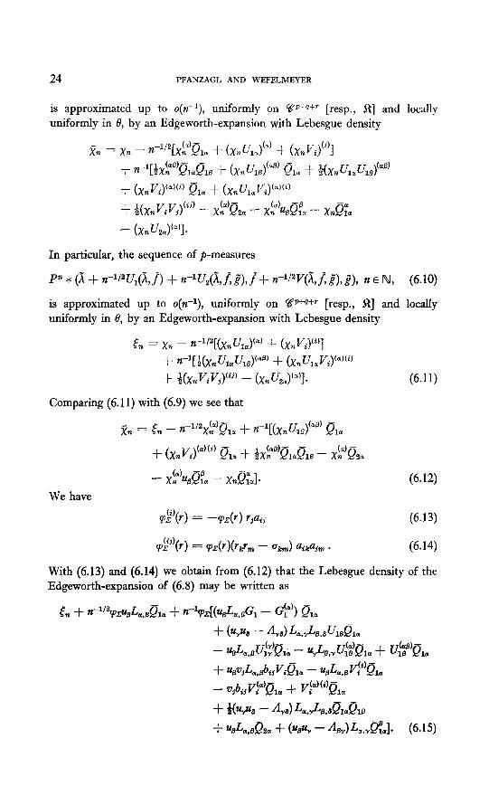
is approximated up to o(n-l), uniformly on ‘@+g+r [resp., 31 and locally uniformly in 8, by an Edgeworth-expansion with Lebesgue density
In particular, the sequence of p-measures
P” * (A + n-Wl(i;,j) + n-‘U,(&J;j),j+ n-‘/“V(X,xg),i), n E N, (6.10)
is approximated up to o(Y+), uniformly on %P+~+r [resp., R] and locally uniformly in 0, by an Edgeworth-expansion with Lebesgue density
62 = xn - +‘2[(xnUla)(=) + (XnVP] + n-y +(& u,, &#=B) + (xn u,, Vp)(i)
+ Q(& v,vp - (xn u2pq.
Comparing (6.11) with (6.9) we see that
(6.11)
We have
vg’(Y) = -vz(Y) YjUij (6.13)
y?‘(Y) = vz(Y)(Y,Y, - Ub) UikUjm s (6.14)
With (6.13) and (6.14) we obtain from (6.12) that the Lebesgue density of the Edgeworth-expansion of (6.8) may be written as
&a + ~-1’2~z~,&,,,~~~ + ~+R&.A,BG, - @)I 810
+ eve - 43 L.J&&B1u
- %L.JJ,‘:‘~lLT - Q$dJ~&x + u$s’pl.
+ U&qVjL, &.V-Q,, - IrsL, *vygj , t3 t
Ql. lol
- v,&, vj4& + vp f*) -
+ H%% - idI 4wAdIu?li3
+ ~&..~~2a + 0~~ - kJLw~~1. (6.15)
MAXIMUM LIKELIHOOD ESTIMATOR 25
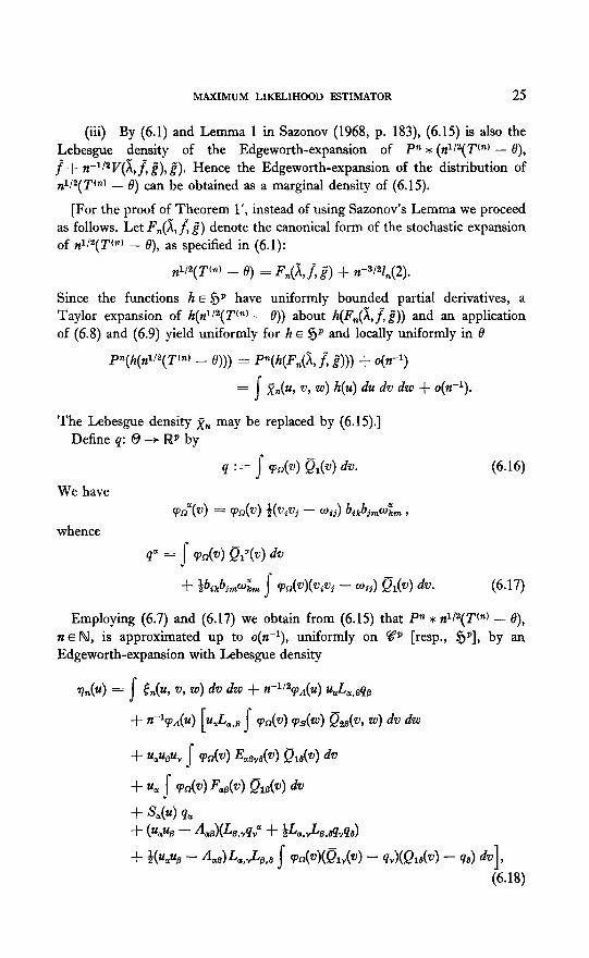
(iii) By (6.1) and L emma 1 in Sazonov (1968, p. 183), (6.15) is also the Lebesgue density of the Edgeworth-expansion of Pn * (n1/2(T(n) - e), fl+ n-1/2V(&f, f), 2). H ence the Edgeworth-expansion of the distribution of G-(P) - 19) can be obtained as a marginal density of (6.15).
[For the proof of Theorem l’, instead of using Sazonov’s Lemma we proceed as follows. Let F,(& f, g”) denote the canonical form of the stochastic expansion of r~l/~(P) - fI), as specified in (6.1):
d/2( T(n) - e) = F,(X,J, 2) + n-3/32,(2).
Since the functions h E SjP have uniformly bounded partial derivatives, a Taylor expansion of Iz(&~(T(“) - 0)) about h(F,(X,J g”)) and an application of (6.8) and (6.9) yield uniformly for h E $p and locally uniformly in 0
~yh(tv(~fn) - e))) = P~(Iz(F,(& f, 2))) + 0(12-l)
= s
&(u, v, w) h(u) du dv dw + o(n-l).
The Lebesgue density xn may be replaced by (6.15).] Define q: 0 -+ Iwr by
q := j- V&J> 8,(v) dv.
We have
whence
(6.16)
+ !&&&n I R&WW - 4 Sk4 dv. (6.17)
Employing (6.7) and (6.17) we obtain from (6.15) that Pn * n112(Vn) - e), n E N, is approximated up to o(n-l), uniformly on %P [resp., 3jp], by an Edgeworth-expansion with Lebesgue density
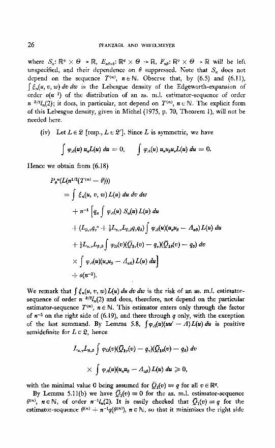
26 PFANZAGL AND WEFELMEYER
where S,: I!@ x 0 + IR, EtiBVs: UP x 0 -+ R, F,,: I@ x 0 + R will be left unspecified, and their dependence on 6 suppressed. Note that S, does not depend on the sequence Vn), n E N. Observe that, by (6.5) and (6.11), s [Ju, v, w) dv dw is the Lebesgue density of the Edgeworth-expansion of order o(n.‘) of the distribution of an as. ml. estimator-sequence of order ~-~l’Y,(2); it does, in particular, not depend on P), n E N. The explicit form of this Lebesgue density, given in Michel (1975, p. 70, Theorem l), will not be needed here.
(iv) Let L E 2 [resp., L E 2’1. Since L is symmetric, we have
Hence we obtain from (6.18)
We remark that s &( u, v, w)L(u) du dv dw is the risk of an as. ml. estimator- sequence of order n-“/“&(2) and d oes, therefore, not depend on the particular estimator-sequence Tf”), n E lV. This estimator enters only through the factor of n-l on the right side of (6.19), and there through 4 only, with the exception of the last summand. By Lemma 5.8, ~~A(~)(uu’ - A) L(u) du is positive semidelinite for L E f!, hence
with the minimal value 0 being assumed for &(v) E 4 for all v E IV. By Lemma 5.1 l(b) we have &(w) E 0 for the as. m.1. estimator-sequence
PI, n E N, of order n-V,(2). It is easily checked that $&(n) I 4 for the estimator-sequence LV) + n-l@(n)), n E fA, so that it minimizes the right side
MAXIMUM LIKELIHOOD ESTIMATOR 27
of (6.19). Furthermore, this estimator-sequence is in 2 [resp., 211. This proves parts (ii) and (iii) of the Theorems.
(v) With H, := {U E UP: U, < 0} we obtain under the assumptions of Theorem 1 from (6.18) for OL = l,...,p
= P,%{@) < 8,) - n--1’y27ry fl;yq, + o(?F2). (6.20)
Hence p is uniquely determined by the median bias of order n-1/2 of !P). This proves Remark 3.14.
ACKNOWLEDGMENTS
The authors wish to thank Mr. K. Michel who worked through earlier versions of the manuscript, and the Deutsche Forschungsgemeinschuft which enabled the cooperation with Mr. Michel by a grant.
Furthermore, the authors are obliged to Mr. F. G&e and Mr. C. Hipp for valuable suggestions in connection with the application of their result on the asymptotic expansion of integrals of smooth functions of sums of i.i.d. variables.
AKAHIRA, M., AND TAKEUCHI, K. (1976a). On the second-order asymptotic efficiencies of estimators. In Proceedings of the Third Japan-USSR Symposium on Probability Theory (G. Maruyama and J. V. Prokhorov, Eds.), pp. 604-638. Lecture Notes in Mathematics 550, Springer-Verlag, Berlin.
AKAHIRA, M., AND TAKEUCHI, K. (1976b). On the second-order asymptotic efficiency of estimators in multiparameter cases, Rep. Uniw. Electra-Comm. 26 261-269.
BAHAIXJR, R. R. (1964). On Fisher’s bound for asymptotic variances. Ann. Math. Statist. 35 1545-1552.
BHATTACHARYA, R. N., AND GHOSH, J. K. (1977). On the validity of the formal Edgeworth expansion. To appear.
BHATTACHARYA, R. N., AND RAO, R. R. (1976). Normal Approximation and Asymptotic Expansions. Wiley, New York.
CHIBISOV, D. M. (1973). An asymptotic expansion for a class of estimators containing maximum likelihood estimators. Theor. Probnbility Appl. 18 295-303.
DH~ADHIKARI, S. W., AND JOGDEO, K. (1976). Multivariate unimodality. Ann. Statist. 4 607-613.
EFRON, B. (1975). Defining the curvature of a statistical problem (with applications to second order efficiency), Ann. Statist. 3 1189-1242.
F&~Y, I., AND RjXnEI, L. (1950). Der zentralsymmetrische Kern und die zentralsymme- trische Htille von konvexen Klirpern. Math. Ann. 122 205-220.
28 PFANZAGL AND WEFELMEYER
GHOSH, J. K., SINHA, B. K., AND WIEAND, H. S. (1977). Second order efficiency of the MLE with respect to any bounded bowl-shaped loss function. To appear.
GHOSH, J. K., AND SUBRAMANYAM; K. (1974). Second-order efficiency of maximum likelihood estimators. Sankhyd Ser. A 36 325-358.
GBTZE, F., AND HIPP, C. (1977). Asymptotic expansions in the central limit theorem under moment conditions. Preprints in Statistics 25. University of Cologne, West Germany.
GUSEV, S. I. (1975). Asymptotic expansions associated with some statistical estimators in the smooth case I. Expansions of random variables. Theor. Probability Appl. 20 470-498.
GUSEV, S. I. (1976). Asymptotic expansions associated with some statistical estimators in the smooth case II. Expansions of moments and distributions. Theor. Probability Appl. 21 14-33.
HAJEK, J. (1970). A characterization of limiting distributions of regular estimates. 2. Wahrscheinlichkeitstheorie und verw. Geb. 14 323-330.
KAUFMAN, S. (1966). Asymptotic efficiency of the maximum likelihood estimator. Ann. Inst. Stat. Math. 18 155-178.
LEHMANN, E. L. (1951). A general concept of unbiasedness. Ann. Math. Statist. 22 587- 592.
MICHEL, R. (1975). An asymptotic expansion for the distribution of asymptotic maximum likelihood estimators of vector parameters. J. Multivariate Anal. 5 67-82.
PFAFF, TH. (1977). Existenz und asymptotische Entwicklungen der Momente mehr- dimensionaler maximum likelihood-Schiitzer, Inaugural-Dissertation, University of Cologne, West Germany.
PFANZAGL, J. (1972). Further results on asymptotic normality I. Metrika 18 174-198. PFANZAGL, J. (1973). Asymptotically optimum estimation and test procedures. In Proceed-
ings of the Prague Symposium on Asymptotic Statistics, Vol. 1 (J. Hdjek, Ed.), pp. 201- 272. Charles University, Prague.
PFANZAGL, J. (1975). On asymptotically complete classes. In Statistical Inference and Related Topics. Proceedings of the Summer Research Institute on Statistical Inference for Stochastic Processes, Vol. 2 (M. L. Puri, Ed.), pp. l-43. Academic Press, New York.
PFANZAGL, J. (1976). First-order efficiency implies second order efficiency, Preprints in Statistics 18. University of Cologne, West Germany. (To appear in the Hbjek Memorial Volume.)
PFANZAGL, J. AND WEFELMEYER, W. (1977). An asymptotically complete class of tests. Preprints in Statistics 24. University of Cologne, West Germany.
PONNAPALLI, R. (1976). Deficiencies of minimum discrepancy estimators. Canad. J. Statist. 4 33-50.
PONNAPALLI, R. (1977). Asymptotic expansions for dispersion matrices of efficient estimators. To appear.
R-40, C. R. (1961). Asymptotic efficiency and limiting information. Proc. Fourth Berkeley Symp. Math. Statist. Prob. I 531-545.
RAO, C. R. (1962). Efficient estimates and optimum inference procedures in large samples. J. Roy. Statist. Sot. Ser. B 24 46-72.
RAO, C. R. (1963). Criteria of estimation in large samples. Sarzkhyti Ser. A 25 189-206.
ROBERTSON, C. A. (1972). On minimum discrepancy estimators. Sankhya Ser. A 34 133-144.
SAZONOV, V. V. (1968). On the multi-dimensional central limit theorem. Sankhyn Ser. A 30 181-204.
MAXIMUM LIKELIHOOD ESTIMATOR 29
SHERMAN, S. (1955). A theorem on convex sets with applications. Arm. Math. Statist. 26 763-767.
STRASSW, H. (1977a). Improved bounds for equivalence of Bayes and maximum likelihood estimation. Tew. Veroj. Pn’men. 22 358-370.
STRM-SER, H. (1977b). Asymptotic expansions for Bayes procedures. In Recent Develop- ments in Statistics (J. R. Barra et aZ., Ed.), pp. 9-35. North-Holland, Amsterdam.