A Three-Scale Model of Spatio-Temporal Bursting

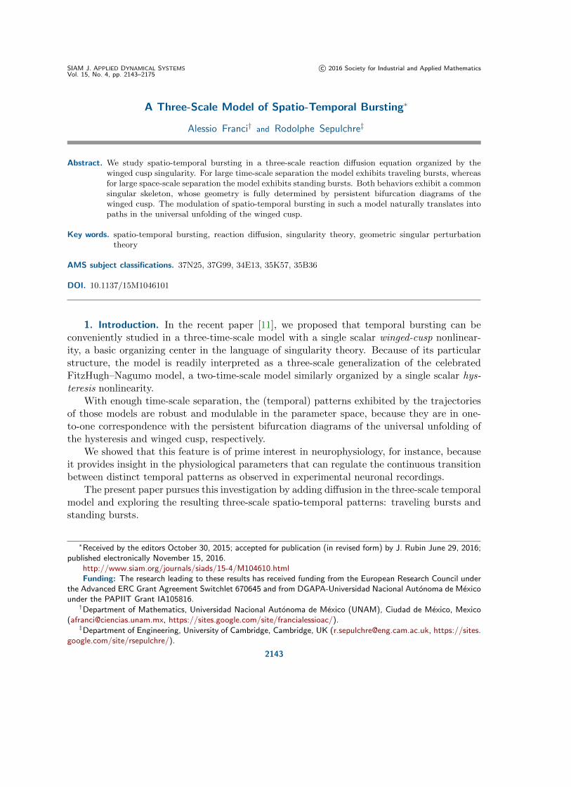
SIAM J. APPLIED DYNAMICAL SYSTEMS c© 2016 Society for Industrial and Applied MathematicsVol. 15, No. 4, pp. 2143–2175

A Three-Scale Model of Spatio-Temporal Bursting∗

Alessio Franci† and Rodolphe Sepulchre‡

Abstract. We study spatio-temporal bursting in a three-scale reaction diffusion equation organized by thewinged cusp singularity. For large time-scale separation the model exhibits traveling bursts, whereasfor large space-scale separation the model exhibits standing bursts. Both behaviors exhibit a commonsingular skeleton, whose geometry is fully determined by persistent bifurcation diagrams of thewinged cusp. The modulation of spatio-temporal bursting in such a model naturally translates intopaths in the universal unfolding of the winged cusp.

Key words. spatio-temporal bursting, reaction diffusion, singularity theory, geometric singular perturbationtheory

AMS subject classifications. 37N25, 37G99, 34E13, 35K57, 35B36

DOI. 10.1137/15M1046101

1. Introduction. In the recent paper [11], we proposed that temporal bursting can beconveniently studied in a three-time-scale model with a single scalar winged-cusp nonlinear-ity, a basic organizing center in the language of singularity theory. Because of its particularstructure, the model is readily interpreted as a three-scale generalization of the celebratedFitzHugh–Nagumo model, a two-time-scale model similarly organized by a single scalar hys-teresis nonlinearity.

With enough time-scale separation, the (temporal) patterns exhibited by the trajectoriesof those models are robust and modulable in the parameter space, because they are in one-to-one correspondence with the persistent bifurcation diagrams of the universal unfolding ofthe hysteresis and winged cusp, respectively.

We showed that this feature is of prime interest in neurophysiology, for instance, becauseit provides insight in the physiological parameters that can regulate the continuous transitionbetween distinct temporal patterns as observed in experimental neuronal recordings.

The present paper pursues this investigation by adding diffusion in the three-scale temporalmodel and exploring the resulting three-scale spatio-temporal patterns: traveling bursts andstanding bursts.

∗Received by the editors October 30, 2015; accepted for publication (in revised form) by J. Rubin June 29, 2016;published electronically November 15, 2016.

http://www.siam.org/journals/siads/15-4/M104610.htmlFunding: The research leading to these results has received funding from the European Research Council under

the Advanced ERC Grant Agreement Switchlet 670645 and from DGAPA-Universidad Nacional Autonoma de Mexicounder the PAPIIT Grant IA105816.†Department of Mathematics, Universidad Nacional Autonoma de Mexico (UNAM), Ciudad de Mexico, Mexico

([email protected], https://sites.google.com/site/francialessioac/).‡Department of Engineering, University of Cambridge, Cambridge, UK ([email protected], https://sites.

google.com/site/rsepulchre/).

2143

http://www.siam.org/journals/siads/15-4/M104610.html

mailto:[email protected]

https://sites.google.com/site/francialessioac/

mailto:[email protected]

https://sites.google.com/site/rsepulchre/

https://sites.google.com/site/rsepulchre/

2144 ALESSIO FRANCI AND RODOLPHE SEPULCHRE

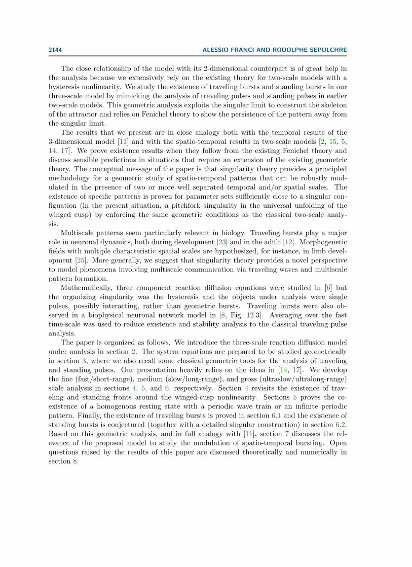
The close relationship of the model with its 2-dimensional counterpart is of great help inthe analysis because we extensively rely on the existing theory for two-scale models with ahysteresis nonlinearity. We study the existence of traveling bursts and standing bursts in ourthree-scale model by mimicking the analysis of traveling pulses and standing pulses in earliertwo-scale models. This geometric analysis exploits the singular limit to construct the skeletonof the attractor and relies on Fenichel theory to show the persistence of the pattern away fromthe singular limit.

The results that we present are in close analogy both with the temporal results of the3-dimensional model [11] and with the spatio-temporal results in two-scale models [2, 15, 5,14, 17]. We prove existence results when they follow from the existing Fenichel theory anddiscuss sensible predictions in situations that require an extension of the existing geometrictheory. The conceptual message of the paper is that singularity theory provides a principledmethodology for a geometric study of spatio-temporal patterns that can be robustly mod-ulated in the presence of two or more well separated temporal and/or spatial scales. Theexistence of specific patterns is proven for parameter sets sufficiently close to a singular con-figuation (in the present situation, a pitchfork singularity in the universal unfolding of thewinged cusp) by enforcing the same geometric conditions as the classical two-scale analy-sis.

Multiscale patterns seem particularly relevant in biology. Traveling bursts play a majorrole in neuronal dynamics, both during development [23] and in the adult [12]. Morphogeneticfields with multiple characteristic spatial scales are hypothesized, for instance, in limb devel-opment [25]. More generally, we suggest that singularity theory provides a novel perspectiveto model phenomena involving multiscale communication via traveling waves and multiscalepattern formation.

Mathematically, three component reaction diffusion equations were studied in [6] butthe organizing singularity was the hysteresis and the objects under analysis were singlepulses, possibly interacting, rather than geometric bursts. Traveling bursts were also ob-served in a biophysical neuronal network model in [8, Fig. 12.3]. Averaging over the fasttime-scale was used to reduce existence and stability analysis to the classical traveling pulseanalysis.

The paper is organized as follows. We introduce the three-scale reaction diffusion modelunder analysis in section 2. The system equations are prepared to be studied geometricallyin section 3, where we also recall some classical geometric tools for the analysis of travelingand standing pulses. Our presentation heavily relies on the ideas in [14, 17]. We developthe fine (fast/short-range), medium (slow/long-range), and gross (ultraslow/ultralong-range)scale analysis in sections 4, 5, and 6, respectively. Section 4 revisits the existence of trav-eling and standing fronts around the winged-cusp nonlinearity. Sections 5 proves the co-existence of a homogenous resting state with a periodic wave train or an infinite periodicpattern. Finally, the existence of traveling bursts is proved in section 6.1 and the existence ofstanding bursts is conjectured (together with a detailed singular construction) in section 6.2.Based on this geometric analysis, and in full analogy with [11], section 7 discusses the rel-evance of the proposed model to study the modulation of spatio-temporal bursting. Openquestions raised by the results of this paper are discussed theoretically and numerically insection 8.

A THREE-SCALE MODEL OF SPATIO-TEMPORAL BURSTING 2145

2. A three-scale reaction diffusion model. The paper studies spatio-temporal burstingin the reaction diffusion model

τuut = Duuxx + gwcusp(u, λ+ w,α+ z, β, γ),(1a)

τwwt = Dwwxx + u− w,(1b)

τzzt = Dzzxx + u− z,(1c)

where τu, τw, τz > 0, Du > 0, and Dw, Dz ≥ 0. The function

gwcusp(u, λ, α, β, γ) = −u3 − λ2 − α+ βu+ γuλ

is a universal unfolding of the winged cusp −u3 − λ2. We regard (1) as a one-componentreaction diffusion model organized by the winged-cusp singularity and with (spatio-temporal)adaptation variables w and z.

The fundamental hypothesis of model (1) is a hierarchy of scales between the “master”variable u and the adaptation variables w and z. This hierarchy of scales is consistent withthe hierarchy between the state variable (u), the bifurcation parameter (λ), and unfoldingparameters (α, β, γ) in singularity theory applied to bifurcation problems [13]. The variable waccounts for variations of the bifurcation parameter while the variable z accounts for variationsof the unfolding parameter α. The fine-grain dynamics is organized by a single nonlinearity,with distinct behaviors depending on the bifurcation parameter and unfolding parameters.The medium-grain dynamics model (linear) adaptation of the bifurcation parameter to thequasi-steady-state of the fine-grain behavior. The gross-grain dynamics models (linear) adap-tation of unfolding parameters to the quasi-steady-state behavior of the fine and mediumgrains.

We study separately the role of a time-scale separation

(2) 0 <τuτz

=: εus �τuτw

=: εs � 1,

which leads to traveling burst waves, and the role of space-scale separation

(3)

√Dz

Du=: δ−1

ul �√Dw

Du=: δ−1

l � 1,

which leads to standing burst waves.The proposed model extends earlier work in two directions:• In the absence of diffusion, model (1) reduces to the bursting model analyzed in [11].

The results in [11] underlie the importance of a persistent bifurcation diagram in theuniversal unfolding of the winged cusp, the mirrored hysteresis (class 2 of the persistentbifurcation diagram of the winged cusp listed in [13, p. 208])), as a key nonlinearity forobtaining robust three-time-scale bursting as ultraslow adaptation around a slow-fastphase portrait with coexistence of a stable fixed point and a stable limit cycle [10].• When the winged-cusp nonlinearity is replaced by an universal unfolding of the hys-

teresis singularity,ghy(u, λ, β) = −x3 + λ+ βx,


then (1) reduces to a FitzHugh–Nagumo-type model, which is the fundamental two-scale model of excitability [9], exhibiting traveling pulses under a time-scale separation[2, 15] and standing pulses under a space-scale separation [5, 17].

3. Methodology.

3.1. Reduction to singularly perturbed ODEs. Using the traveling wave anszatz (u,w, z)( x√

Du+ c t

τu), traveling and standing waves of (1) satisfy the ODE

u′ = vu ,(4a)

v′u = cvu − gwcusp(u, λ+ w,α+ z, β, γ) ,(4b)

w′ = vw ,(4c)

v′w = cδ2l

εsvw + δ2

l (w − u) ,(4d)

z′ = vz ,(4e)

v′z = cδ2ul

εusvz + δ2

ul(z − u) .(4f)

For Dw, Dz 6= 0, we set c = 0 and use the change of variables vw 7→ vwδl, vz 7→ vz

δulto study

the existence of standing waves satisfying the ODE

u′ = vu ,(5a)

v′u = −gwcusp(u, λ+ w,α+ z, β, γ) ,(5b)

w′ = δlvw ,(5c)

v′w = δl(w − u) ,(5d)

z′ = δulvz ,(5e)

v′z = δul(z − u) .(5f)

To study traveling waves, we start by multiplying both sides of (4d) and (4f) by εscδ2l

andεuscδ2ul

, respectively,

u′ = vu ,

v′u = cvu − gwcusp(u, λ+ w,α+ z, β, γ) ,

w′ = vw ,εscδ2l

v′w = vw +εsc

(w − u) ,

z′ = vz ,εuscδ2ul

v′z = vz +εusc

(z − u) .


In the limit εscδ2l, εuscδ2ul→ 0, we obtain

u′ = vu ,(6a)

v′u = cvu − gwcusp(u, λ+ w,α+ z, β, γ) ,(6b)

w′ =εsc

(u− w) ,(6c)

z′ =εusc

(u− z) .(6d)

Note that if Dw = Dz = 0, that is, the two adaptation variable do not diffuse, then εscδ2l, εuscδ2ul

=

0, because in this case δl = δul = +∞. The persistence of the limit εscδ2l, εuscδ2ul→ 0 for Dw, Dz 6= 0

will not be addressed in the present paper but we verify it numerically in section 8.2.1.

3.2. The geometry of traveling and standing pulses. For future reference, we brieflyrecall here the geometric construction of traveling and standing pulses in two-scale reactiondiffusion equations. Our exposition is based on [14, sections 4.2, 4.5, and 5.3] for the travelingcase and [17, sections 4 and 5], [5, section 2] for the standing case.

Let ghy(u, λ, β) = −u3 + βu + λ be an universal unfolding of the hysteresis singularity.The two-scale reaction diffusion model

τuut = Duuxx + ghy(u, λ+ w, β),(7a)

τwwt = Dwwxx + u− w,(7b)

exhibits traveling pulses under time-scale separation (2) and standing pulses under space-scaleseparation (3). The traveling pulse is constructed geometrically for Dw = 0 using the travelingwave ansatz. The standing pulse is constructed geometrically in the traveling wave ansatzwith c = 0. For large time-scale separation and large space-scale separation the two reductionslead to the singularly perturbed ODEs

u′ = vu ,(8a)

v′u = cvu − ghy(u, λ+ w, β),(8b)

w′ =εsc

(u− w) ,(8c)

c′ = 0 ,(8d)

(traveling)

u′ = vu ,(9a)

v′u = −ghy(u, λ+ w, β),(9b)

w′ = δlvw ,(9c)

v′w = δl(w − u) .(9d)

(standing)

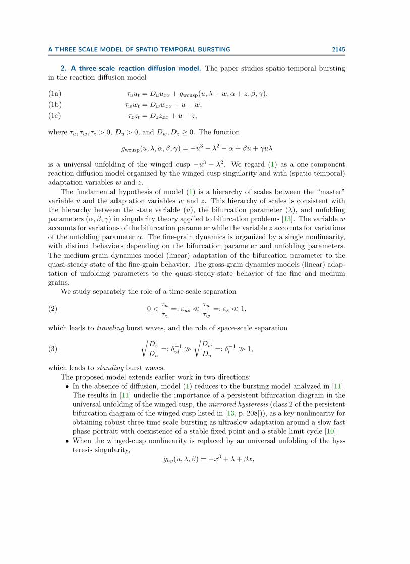
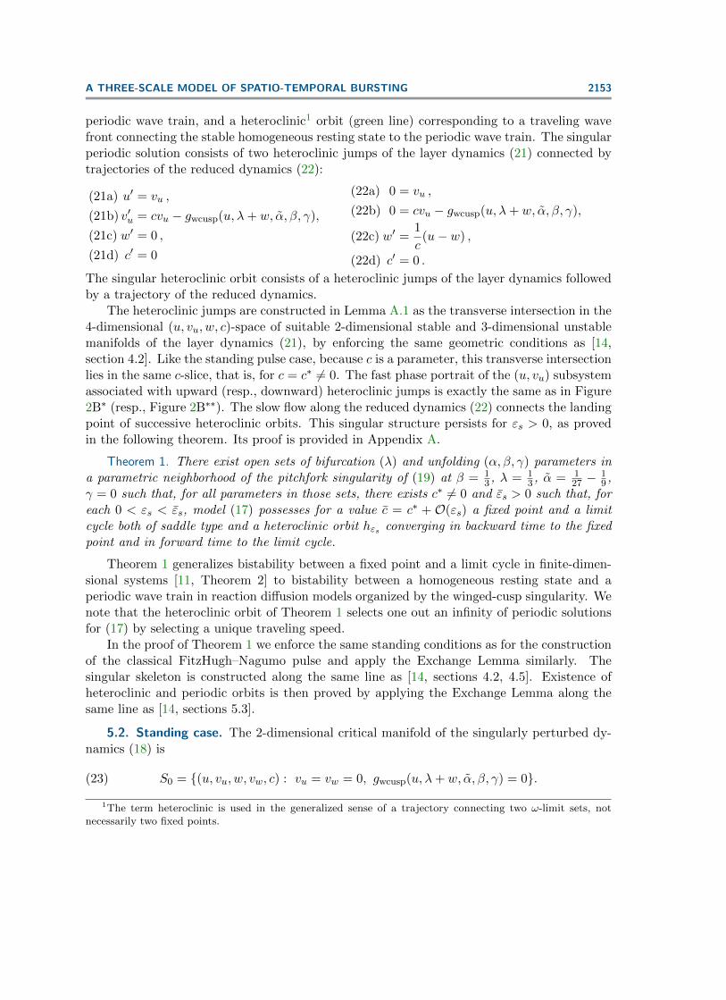
The dummy dynamics of the wave speed parameter c in the traveling case is needed forthe singular perturbation construction. Under the same geometric conditions as [14, sec-tion 4.2]—traveling case—and [5, section 1]—standing case—the singular skeleton of (8) and(9) is sketched in Figure 1. Geometrically, traveling and standing pulses share the samesingular skeleton provided by their hysteretic critical manifold

S0 = {(u, vu, w, c) : vu = 0, ghy(u, λ+ w, β) = 0}(traveling),

S0 = {(u, vu, w, vw) : vu = vw = 0, ghy(u, λ+ w, β) = 0}(standing).


u

w w

Traveling pulseu

Standing pulse

w

u

vw

w

u

vw

*

*

**

**

(u ,u )rest rest

(u ,u )rest rest

S0 S0

Figure 1. Geometry of traveling and standing pulses in reaction diffusion model with a cubic nonlinearity.Stable homogeneous resting states are depicted as black dots. The critical manifold S0 is depicted as the thickblack line. The thin black line is the nullcline of the slow variable w (traveling case) or vw (standing case).Trajectories of the layer dynamics (10) and (13) are drawn with double arrows. Trajectories of the reduceddynamics (11) and (12) are drawn with single arrows.

Both traveling and standing pulses are constructed as homoclinic orbits obtained as per-turbations of the singular homoclinic orbits sketeched in Figure 1.

The singular homoclinic orbit associated with the traveling pulse begins with a first jumpfrom steady state to the excited along the (fast) layer dynamics

u′ = vu ,(10a)

v′u = cvu − ghy(u, λ+ w, β) ,(10b)

w′ = 0 ,(10c)

c′ = 0 .(10d)

This jump is a heteroclinic orbit of (10) constructed as the transverse intersection in the4-dimensional (u, vu, w, c)-space of suitable 2-dimensional stable and 3-dimensional unstablemanifolds (see [14, section 4.5] for details). Because c is a parameter, this transverse inter-section lies in the same c-slice, that is, for c = c∗ 6= 0. The phase portrait of the (u, vu)subsystem at the heteroclinic connection is the same as Figure 2B∗∗. The slow motion insidethe 1-dimensional c = c∗-slice of the upper branch of the critical manifold is ruled by thereduced dynamics

0 = vu ,(11a)

0 = cvu − ghy(u, λ+ w, β) ,(11b)

w′ =1

c(u− w) ,(11c)

c′ = 0, c = c∗ .(11d)


u

vu

u

vu

u

Traveling frontsu

Standing fronts

vu

u

u

λ~

A)

B)

*

**

* ** ***

****

**

*** ***w w

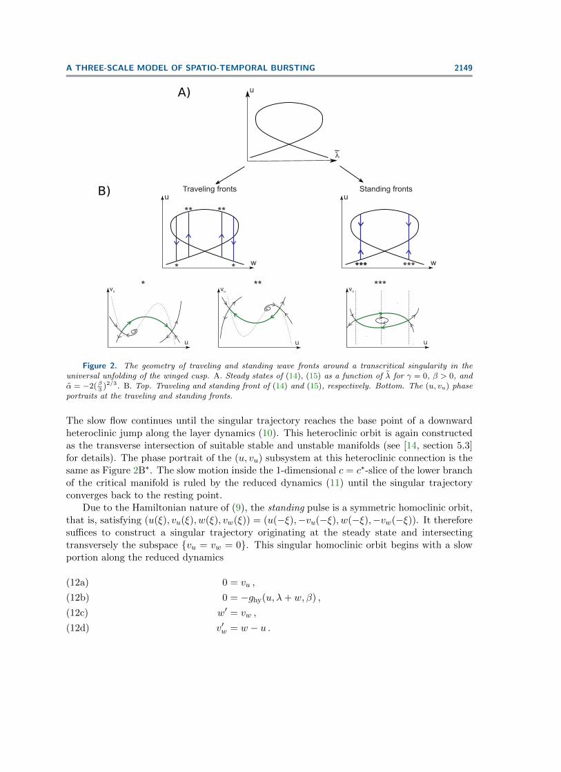
Figure 2. The geometry of traveling and standing wave fronts around a transcritical singularity in theuniversal unfolding of the winged cusp. A. Steady states of (14), (15) as a function of λ for γ = 0, β > 0, andα = −2(β

3)2/3. B. Top. Traveling and standing front of (14) and (15), respectively. Bottom. The (u, vu) phase

portraits at the traveling and standing fronts.

The slow flow continues until the singular trajectory reaches the base point of a downwardheteroclinic jump along the layer dynamics (10). This heteroclinic orbit is again constructedas the transverse intersection of suitable stable and unstable manifolds (see [14, section 5.3]for details). The phase portrait of the (u, vu) subsystem at this heteroclinic connection is thesame as Figure 2B∗. The slow motion inside the 1-dimensional c = c∗-slice of the lower branchof the critical manifold is ruled by the reduced dynamics (11) until the singular trajectoryconverges back to the resting point.

Due to the Hamiltonian nature of (9), the standing pulse is a symmetric homoclinic orbit,that is, satisfying (u(ξ), vu(ξ), w(ξ), vw(ξ)) = (u(−ξ),−vu(−ξ), w(−ξ),−vw(−ξ)). It thereforesuffices to construct a singular trajectory originating at the steady state and intersectingtransversely the subspace {vu = vw = 0}. This singular homoclinic orbit begins with a slowportion along the reduced dynamics

0 = vu ,(12a)

0 = −ghy(u, λ+ w, β) ,(12b)

w′ = vw ,(12c)

v′w = w − u .(12d)


Because v′w > 0 on the right of the steady state, vw and, therefore, also w, increase until thetrajectory reaches the base point of a heteroclinic trajectory along the layer dynamics

u′ = vu ,(13a)

v′u = −ghy(u, λ+ w, β) ,(13b)

w′ = 0,(13c)

v′w = 0.(13d)

Existence of this heteroclinic orbit easily follows from the Hamiltonian nature of the layer dy-namics. The fact that it can be constructed as the transverse intersection in the 4-dimensional(u, vu, w, vw)-space of suitable 2-dimensional stable and 3-dimensional unstable manifolds isproved by imposing the geometric conditions in [5, section 1]. At the heteroclinic jump thetrajectory jumps to the upper branch of the critical manifold. There, the trajectory is carriedtransversely across {vu = vw = 0} by the reduced flow (12). Again, transversality, in particu-lar the fact that the trajectory remains bounded away from the fold singularity of the criticalmanifold, is proved by imposing the geometric conditions in [5, section 1]. The other half ofthe trajectory is constructed by symmetry.

Persistence of the singular homoclinic orbits associated with both the traveling and stand-ing pulse follows by the Exchange Lemma [16]. Roughly speaking, the Exchange Lemma allowsus to track, for ε > 0, the invariant (stable and unstable) manifolds involved in the construc-tion of the singular orbits and, in particular, to ensure that the same transverse intersectionspersist away from the singular limit and for ε sufficiently small.

Application of the Exchange Lemma in the construction of the classical traveling andstanding pulse requires that the homoclinic trajectory solely shadows a normally hyperbolicpart of the critical manifold. In the traveling case, this property is enforced by the fact thatthe homogeneous resting state is far from the fold singularity (note that the property mayfail to hold when the resting state is close to the fold singularity or when ε becomes too large[3]). In the standing case it is enforced by the geometric assumptions in [5, section 1]. Wewill enforce the same property in the construction of our traveling and standing bursts byenforcing similar geometric conditions as the classical traveling and standing pulse.

4. Fine-scale analysis: Bistability and connecting fronts. For εs = εus = 0 and δl =δul = 0, models (6) and (5) reduce to one-scale behaviors describing the fine-grain dynamics:

u′ = vu ,(14a)

v′u = cvu − gwcusp(u, λ, α, β, γ)(14b)

(traveling),

u′ = vu ,(15a)

v′u = −gwcusp(u, λ, α, β, γ)(15b)

(standing),

where λ, α, c, w, and z are now fixed parameters.In both models, the steady-states

(16) {(u, vu) : vu = 0, gwcusp(u, λ, α, β, γ) = 0}

are determined by the universal unfolding of the winged cusp, as the bifurcation and unfoldingparameters vary. For γ = 0, β > 0, and α = −2(β3 )2/3, the steady-state curve possesses a


transcritical singularity for λ = 0, where two mirror-symmetric hysteretic branches merge, assketched in Figure 2A.

Away from the transcritical singularity, both hysteretic branches possess the same quali-tative geometry as the classical cubic critical manifold in Figure 1. In particular, they exhibitbistability between up and down homogeneous steady states of the associated scalar reactiondiffusion equation. Both in the traveling and standing case, there exist connecting heteroclinicorbits between the up and down steady-state branches (Figure 2B), which correspond to trav-eling or standing wave fronts of the associated reaction diffusion equation. In the travelingcase, there are four c-dependent values of the bifurcation parameter λ for which the modelposses a heteroclinic orbit: two upward heteroclinic orbits and two downward heteroclinicorbits. In the standing case, there are two values of the bifurcation parameter λ for which themodel possesses both a downward and an upward heteroclinic orbit. The phase portraits ofthe fast heteroclinic jumps are sketched in the insets.

Existence of these heteroclinic orbits follows exactly from the theory in [14, section 4.5] forthe traveling case and in [17, section 4] for the standing case. They all persist to parametervariations, in particular, to unfolding of the transcritical singularity. We omit here a detailedproof but the key derivations are recalled in Lemma A.1 for the traveling case and in LemmaB.1 for the standing case.

5. Medium-scale analysis: Bistability between homogeneous and periodic states. Tomodel slow adaptation of the bifurcation parameter λ, we unfreeze the slow variable w andstudy coexistence of a resting state (corresponding to a stable homogeneous resting state inthe original PDE) and a limit cycle (corresponding to a periodic wave train or an infiniteperiodic patter in the original PDE) in the models:

u′ = vu ,(17a)

v′u = cvu − gwcusp(u, λ+ w, α, β, γ),(17b)

w′ =εsc

(u− w) ,(17c)

c′ = 0(17d)

(traveling),

u′ = vu ,(18a)

v′u = −gwcusp(u, λ+ w, α, β, γ),(18b)

w′ = δlvw ,(18c)

v′w = δl(w − u)(18d)

(standing),

for εs and δl sufficiently small, respectively. This bistability is the generalization of bistabilitybetween the homogeneous rest and excited states in the two-scale scenario.

For future reference, we make the following preliminary observation. The homogeneousresting state equation of (17) and (18) is

(19) F (u, λ, α, β, γ) := −u3 − (λ+ u)2 + βu− γ(λ+ u)u− α = 0

and is easily shown to be again a universal unfolding of the winged cusp around uwcusp := 13 ,

λwcusp := 0, αwcusp := − 127 , βwcusp := −1

3 , γwcusp := −2.

5.1. Traveling case. The 2-dimensional critical manifold of the singularly perturbed dy-namics (17) is

(20) S0 = {(u, vu, w, c) : vu = 0, gwcusp(u, λ+ w, α, β, γ) = 0}.


u

w

Traveling Standing

(u ,u )rest rest

(u ,u )rest rest

u

w

u

w

vw

A) B1)

B2)

S0

S0

S0

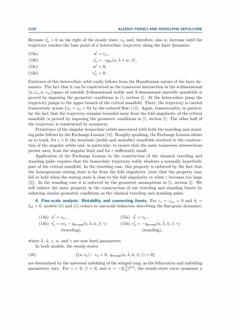
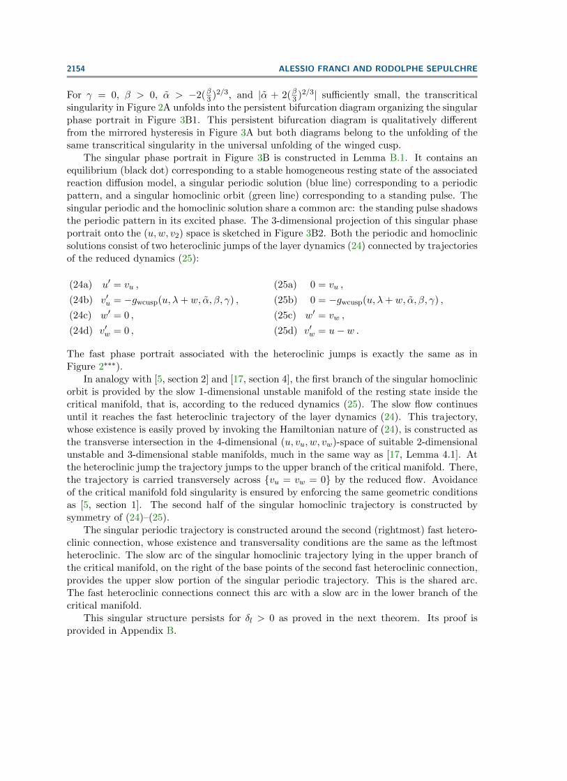
Figure 3. A. Bistability between a homogeneous steady state and a periodic wave train in the singular limitand in the traveling wave ansatz. The two objects are connected by a traveling front. The homogeneous restingstate is depicted as a black dot, the singular heteroclinic orbit corresponding to the traveling front as a greenoriented line, and the singular periodic orbit corresponding to the periodic wave train as a blue oriented line.One arrow indicates slow portions along the reduced dynamics (22), two arrows fast portions along the layerdynamics (21). B. Bistability between a homogeneous steady state and an infinite periodic pattern in the singularlimit and in the standing wave ansatz. There is also a (single) standing pulse solution that shadows the periodicpattern. The homogeneous resting state is depicted as a black dot, the singular periodic orbit correspondingto the infinite periodic pattern as a blue oriented line, and the singular homoclinic orbit corresponding to thestanding pulse as a green oriented line. One arrow indicates slow portions along the reduced dynamics (25),two arrows fast portions along the layer dynamics (24).

For γ = 0, β > 0, and α < −2(β3 )2/3 the transcritical singularity in Figure 2A unfoldsinto the mirrored hysteresis persistent bifurcation diagram introduced in [11, section 2.3] andorganizing the singular phase portrait in Figure 3A. This algebraic curve is a template forrest-spike bistability in ODEs [10, Theorem 2]. Here we show that it is also a template toconstruct a wavefront between homogeneous resting and a periodic wave train.

The singular phase portrait of (17) in Figure 3A is constructed in Lemma A.1. It existsfor a precise value c = c∗ derived along the same line as [14, section 4.2]. It contains anequilibrium (black dot) corresponding to a stable homogeneous resting state of the associatedreaction diffusion model, a singular periodic solution (blue line) corresponding to a traveling


periodic wave train, and a heteroclinic1 orbit (green line) corresponding to a traveling wavefront connecting the stable homogeneous resting state to the periodic wave train. The singularperiodic solution consists of two heteroclinic jumps of the layer dynamics (21) connected bytrajectories of the reduced dynamics (22):

u′ = vu ,(21a)

v′u = cvu − gwcusp(u, λ+ w, α, β, γ),(21b)

w′ = 0 ,(21c)

c′ = 0(21d)

0 = vu ,(22a)

0 = cvu − gwcusp(u, λ+ w, α, β, γ),(22b)

w′ =1

c(u− w) ,(22c)

c′ = 0 .(22d)

The singular heteroclinic orbit consists of a heteroclinic jumps of the layer dynamics followedby a trajectory of the reduced dynamics.

The heteroclinic jumps are constructed in Lemma A.1 as the transverse intersection in the4-dimensional (u, vu, w, c)-space of suitable 2-dimensional stable and 3-dimensional unstablemanifolds of the layer dynamics (21), by enforcing the same geometric conditions as [14,section 4.2]. Like the standing pulse case, because c is a parameter, this transverse intersectionlies in the same c-slice, that is, for c = c∗ 6= 0. The fast phase portrait of the (u, vu) subsystemassociated with upward (resp., downward) heteroclinic jumps is exactly the same as in Figure2B∗ (resp., Figure 2B∗∗). The slow flow along the reduced dynamics (22) connects the landingpoint of successive heteroclinic orbits. This singular structure persists for εs > 0, as provedin the following theorem. Its proof is provided in Appendix A.

Theorem 1. There exist open sets of bifurcation (λ) and unfolding (α, β, γ) parameters ina parametric neighborhood of the pitchfork singularity of (19) at β = 1

3 , λ = 13 , α = 1

27 −19 ,

γ = 0 such that, for all parameters in those sets, there exists c∗ 6= 0 and εs > 0 such that, foreach 0 < εs < εs, model (17) possesses for a value c = c∗ + O(εs) a fixed point and a limitcycle both of saddle type and a heteroclinic orbit hεs converging in backward time to the fixedpoint and in forward time to the limit cycle.

Theorem 1 generalizes bistability between a fixed point and a limit cycle in finite-dimen-sional systems [11, Theorem 2] to bistability between a homogeneous resting state and aperiodic wave train in reaction diffusion models organized by the winged-cusp singularity. Wenote that the heteroclinic orbit of Theorem 1 selects one out an infinity of periodic solutionsfor (17) by selecting a unique traveling speed.

In the proof of Theorem 1 we enforce the same standing conditions as for the constructionof the classical FitzHugh–Nagumo pulse and apply the Exchange Lemma similarly. Thesingular skeleton is constructed along the same line as [14, sections 4.2, 4.5]. Existence ofheteroclinic and periodic orbits is then proved by applying the Exchange Lemma along thesame line as [14, sections 5.3].

5.2. Standing case. The 2-dimensional critical manifold of the singularly perturbed dy-namics (18) is

(23) S0 = {(u, vu, w, vw, c) : vu = vw = 0, gwcusp(u, λ+ w, α, β, γ) = 0}.

1The term heteroclinic is used in the generalized sense of a trajectory connecting two ω-limit sets, notnecessarily two fixed points.


For γ = 0, β > 0, α > −2(β3 )2/3, and |α + 2(β3 )2/3| sufficiently small, the transcriticalsingularity in Figure 2A unfolds into the persistent bifurcation diagram organizing the singularphase portrait in Figure 3B1. This persistent bifurcation diagram is qualitatively differentfrom the mirrored hysteresis in Figure 3A but both diagrams belong to the unfolding of thesame transcritical singularity in the universal unfolding of the winged cusp.

The singular phase portrait in Figure 3B is constructed in Lemma B.1. It contains anequilibrium (black dot) corresponding to a stable homogeneous resting state of the associatedreaction diffusion model, a singular periodic solution (blue line) corresponding to a periodicpattern, and a singular homoclinic orbit (green line) corresponding to a standing pulse. Thesingular periodic and the homoclinic solution share a common arc: the standing pulse shadowsthe periodic pattern in its excited phase. The 3-dimensional projection of this singular phaseportrait onto the (u,w, v2) space is sketched in Figure 3B2. Both the periodic and homoclinicsolutions consist of two heteroclinic jumps of the layer dynamics (24) connected by trajectoriesof the reduced dynamics (25):

u′ = vu ,(24a)

v′u = −gwcusp(u, λ+ w, α, β, γ) ,(24b)

w′ = 0 ,(24c)

v′w = 0 ,(24d)

0 = vu ,(25a)

0 = −gwcusp(u, λ+ w, α, β, γ) ,(25b)

w′ = vw ,(25c)

v′w = u− w .(25d)

The fast phase portrait associated with the heteroclinic jumps is exactly the same as inFigure 2∗∗∗).

In analogy with [5, section 2] and [17, section 4], the first branch of the singular homoclinicorbit is provided by the slow 1-dimensional unstable manifold of the resting state inside thecritical manifold, that is, according to the reduced dynamics (25). The slow flow continuesuntil it reaches the fast heteroclinic trajectory of the layer dynamics (24). This trajectory,whose existence is easily proved by invoking the Hamiltonian nature of (24), is constructed asthe transverse intersection in the 4-dimensional (u, vu, w, vw)-space of suitable 2-dimensionalunstable and 3-dimensional stable manifolds, much in the same way as [17, Lemma 4.1]. Atthe heteroclinic jump the trajectory jumps to the upper branch of the critical manifold. There,the trajectory is carried transversely across {vu = vw = 0} by the reduced flow. Avoidanceof the critical manifold fold singularity is ensured by enforcing the same geometric conditionsas [5, section 1]. The second half of the singular homoclinic trajectory is constructed bysymmetry of (24)–(25).

The singular periodic trajectory is constructed around the second (rightmost) fast hetero-clinic connection, whose existence and transversality conditions are the same as the leftmostheteroclinic. The slow arc of the singular homoclinic trajectory lying in the upper branch ofthe critical manifold, on the right of the base points of the second fast heteroclinic connection,provides the upper slow portion of the singular periodic trajectory. This is the shared arc.The fast heteroclinic connections connect this arc with a slow arc in the lower branch of thecritical manifold.

This singular structure persists for δl > 0 as proved in the next theorem. Its proof isprovided in Appendix B.


Theorem 2. There exist open sets of bifurcation (λ) and unfolding (α, β, γ) parameters in aparametric neighborhood of the pitchfork singularity of (19) at β = 1

3 , λ = 13 , α = 1

27−19 , γ = 0

such that, for all parameters in those sets, there exists δl > 0 such that, for all 0 < δl < δl,model (18) possesses a homoclinic trajectory and a limit cycle that are O(δl)-close to eachother together with their unstable manifolds in a neighborhood of the point (umax, 0, wmax, 0),where w reaches its (unique) maximum along the singular homoclinic trajectory.

Theorem 2 characterizes bistability between a homogeneous resting state and a periodicpattern in reaction diffusion models organized by the winged-cusp singularity. We note thatthe homoclinic orbit singles out a privileged periodic pattern in model (18) out of an infinityof them.

In the proof of Theorem 2 we enforce the same conditions as the construction of thestanding pulse and use the Exchange Lemma similarly. The singular skeleton is constructedby enforcing the same assumptions as [5, section 2]. The existence of the homoclinic andperiodic orbits is proved along the same lines as [17, sections 4 and 5].

6. Gross scale analysis: Traveling and standing bursts.

6.1. Traveling bursts. Very much like traveling pulses are homoclinic orbits of the sin-gularly perturbed dynamics (8), traveling bursts are constructed as homoclinic orbits of thesingularly perturbed dynamics (6). We start by constructing the singular limit εs → 0 of thishomoclinic orbit under the assumption that εus = εusεs with 0 < εus � 1. The layer (26) andreduced (27) dynamics then read

u′ = v ,(26a)

v′ = cv −gwcusp(u, λ+ w,α+ z, β, γ),(26b)

w′ = 0 ,(26c)

z′ = 0 ,(26d)

c′ = 0 ,(26e)

0 = v ,(27a)

0 = cv −gwcusp(u, λ+ w,α+ z, β, γ),(27b)

w′ =1

c(u− w) ,(27c)

z′ =εusc

(u− z) ,(27d)

c′ = 0 .(27e)

The associated critical manifold is

(28) S0 := {(u, v, w, z, c) : v = 0, gwcusp(u, λ+ w,α+ z, β, γ) = 0}.

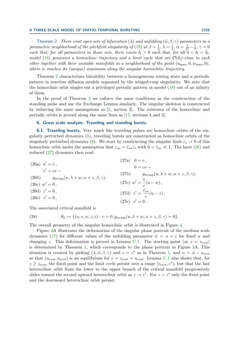
The overall geometry of the singular homoclinic orbit is illustrated in Figure 4.Figure 4A illustrates the deformation of the singular phase portrait of the medium scale

dynamics (17) for different values of the unfolding parameter α = α + z for fixed α andchanging z. This deformation is proved in Lemma C.1. The starting point (at z = zrest)is determined by Theorem 1, which corresponds to the phase portrait in Figure 3A. Thissituation is created by picking (λ, α, β, γ) and c = c∗ as in Theorem 1, and α = α − urestso that (urest, urest) is an equilibrium for z = zrest = urest. Lemma C.1 also shows that, forz ≥ zrest, the fixed point and the limit cycle persist over a range [zrest, z

∗), but that the fastheteroclinic orbit from the lower to the upper branch of the critical manifold progressivelyslides toward the second upward heteroclinic orbit as z → z∗. For z > z∗ only the fixed pointand the downward heteroclinic orbit persist.


z

u

w

z

(urest,urest,urest)S0

z *

zrest=urest

A)

B)

(urest,urest)

Figure 4. Geometric construction of traveling bursts. A. Deformation of the slow-fast phase portrait of (17)for different values of α = α+ z for fixed α and different values of z. Notation as in Figure 3. B. Projection ofthe singular homoclinic orbit corresponding to the traveling burst solution (in red) onto the (u,w, z) space. Onearrow indicates slow portions along the layer dynamics (27), two arrows fast portions along the layer dynamics(26). Base and landing points of the fast heteroclinic connections lie along the blue lines.

The singular homoclinic orbit is constructed by gluing together the z-slices of Figure 4Ain the range [zrest, z

∗ + θ] for small θ > 0, as illustrated in Figure 4B. As for the travelingpulse, a first heteroclinic jump brings the orbit from rest to the excited state. As z increasesin the ultraslow scale, the slow flow governed by (27) brings the trajectory to the base pointof the next fast heteroclinic jump. The alternation of slow flows and fast heteroclinic jumps,along the family of singular limit cycles, continues until z > z∗. The orbit then relaxes backto rest along the lower branch of the critical manifold.

The following theorem proves the existence of a homoclinic orbit that tracks the singularhomoclinic orbit away from the singular limit. Its proof is provided in Appendix C.


Theorem 3. There exist open sets of bifurcation (λ) and unfolding (α, β, γ) parameters ina parametric neighborhood of the pitchfork singularity of (19) at β = 1

3 , λ = 13 , α = 1

27 −19 ,

γ = 0 such that, for all parameters in those sets, there exists c∗ 6= 0 such that for almostall εus > 0 sufficiently small and c = c∗, the singular limit (26)–(27) possesses a transversesingular homoclinic orbit as sketched in Figure 4. Furthermore, model (6) possesses for εs > 0sufficiently small a homoclinic orbit near the transverse singular homoclinic orbit.

The proof of Theorem 3 is a direct application of the Exchange Lemma, more precisely, ofthe theorem in [16, section 4], which applies the Exchange Lemma to persistence of singularhomoclinic orbits like the one in Figure 4. The presence of a third scale governed by εus or,equivalently, by εus is solely exploited to enforce the transversality conditions required by theapplication of the Exchange Lemma to (8) via the singular limit (26)–(27). Genericity in εusarises by imposing some of these transversality conditions.

Nongeneric values of εus include spike-adding bifurcations in which the number of spikesper burst in the singular homoclinic solution changes: for εus sufficiently large there is onlyone spike per burst because the slow flow brings z above z∗ after just one jump; for decreasingεus the number of jumps necessary to bring z above z∗ increases monotonically and so doesthe number of spikes per burst. Spike-adding bifurcations and the rich dynamics they bringare well known in the purely temporal saddle-homoclinic bursting setting (see, e.g., [20, 22]).

6.2. Standing bursts. In analogy with the standing pulses of (9), the standing bursts ofthe singularly perturbed dynamics (5) are symmetric homoclinic orbits, that is, they satisfy

(u(ξ), vu(ξ), w(ξ), vw(ξ), z(ξ), vz(ξ)) = (u(−ξ),−vu(−ξ), w(−ξ),−vw(−ξ), z(−ξ),−vz(−ξ)).

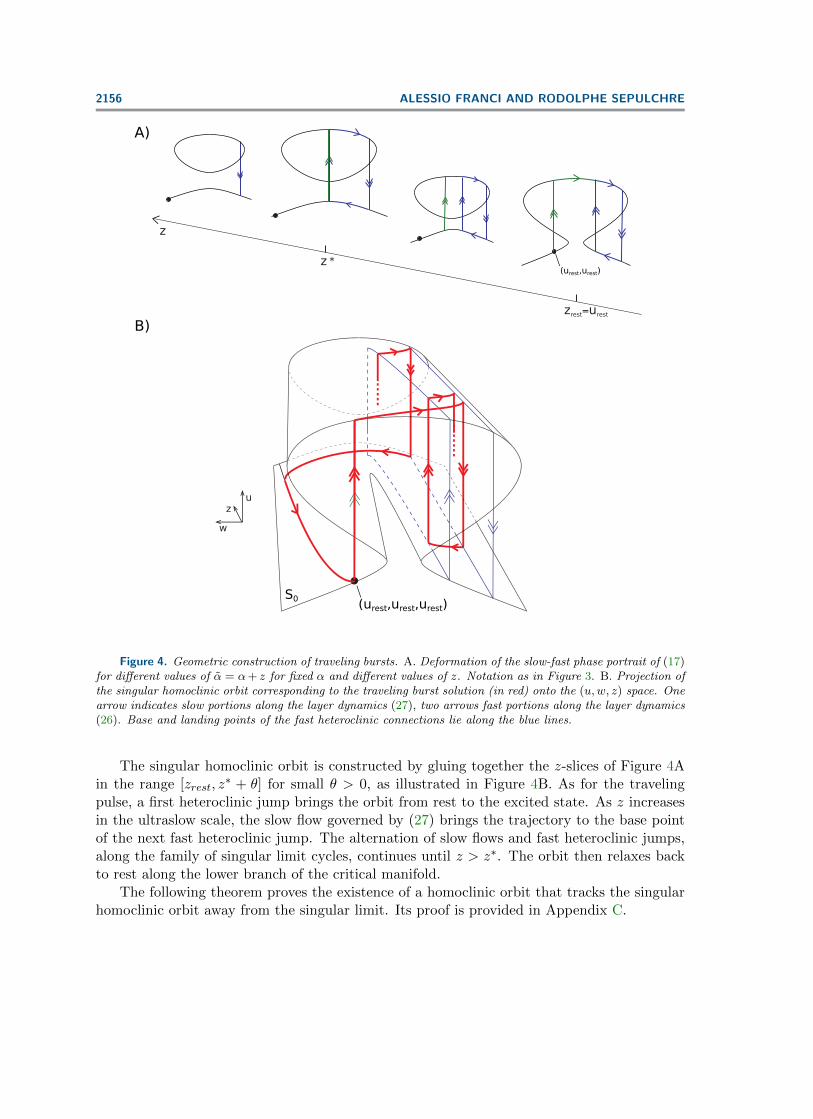
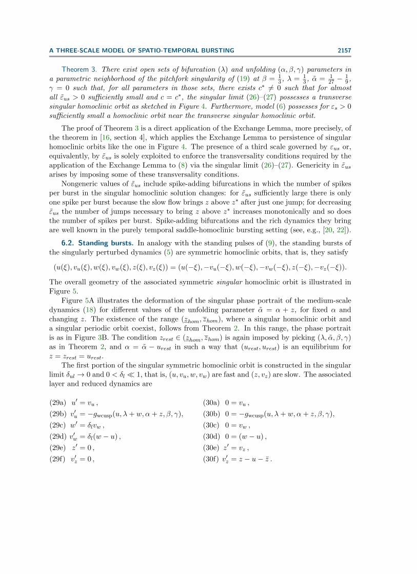
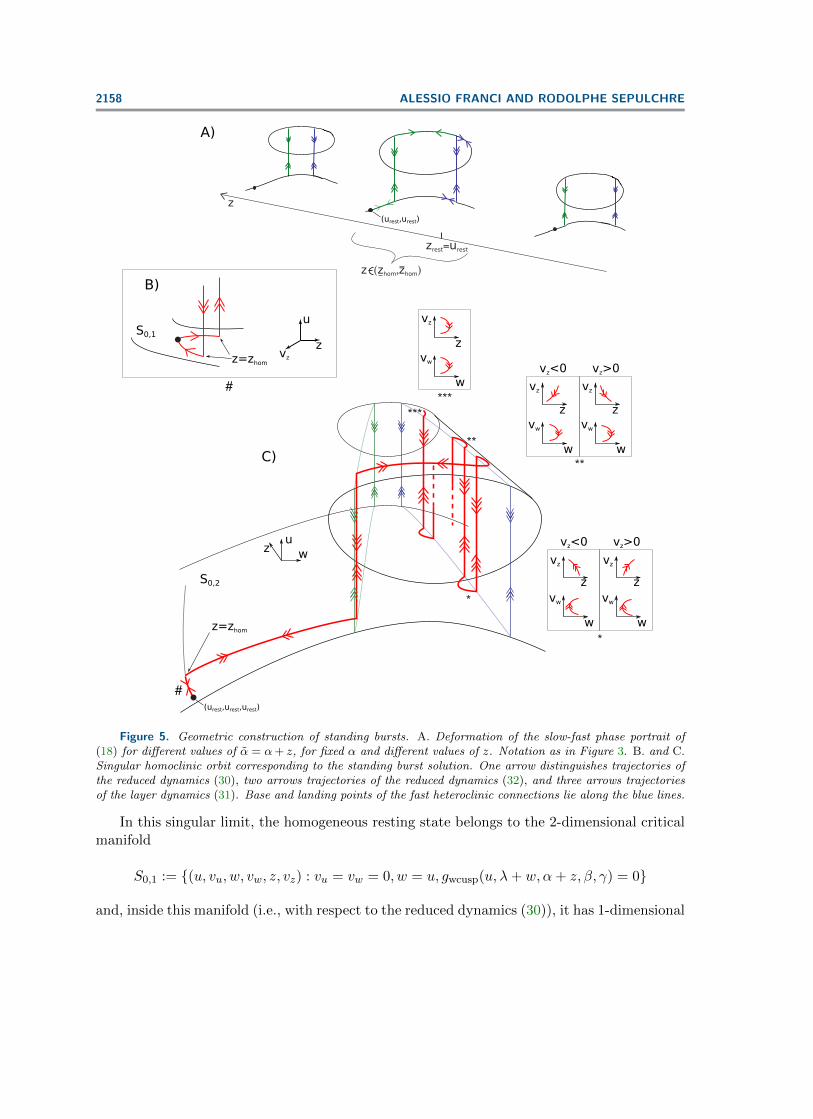
The overall geometry of the associated symmetric singular homoclinic orbit is illustrated inFigure 5.

Figure 5A illustrates the deformation of the singular phase portrait of the medium-scaledynamics (18) for different values of the unfolding parameter α = α + z, for fixed α andchanging z. The existence of the range (zhom, zhom), where a singular homoclinic orbit anda singular periodic orbit coexist, follows from Theorem 2. In this range, the phase portraitis as in Figure 3B. The condition zrest ∈ (zhom, zhom) is again imposed by picking (λ, α, β, γ)as in Theorem 2, and α = α − urest in such a way that (urest, urest) is an equilibrium forz = zrest = urest.

The first portion of the singular symmetric homoclinic orbit is constructed in the singularlimit δul → 0 and 0 < δl � 1, that is, (u, vu, w, vw) are fast and (z, vz) are slow. The associatedlayer and reduced dynamics are

u′ = vu ,(29a)

v′u = −gwcusp(u, λ+ w,α+ z, β, γ),(29b)

w′ = δlvw ,(29c)

v′w = δl(w − u) ,(29d)

z′ = 0 ,(29e)

v′z = 0 ,(29f)

0 = vu ,(30a)

0 = −gwcusp(u, λ+ w,α+ z, β, γ),(30b)

0 = vw ,(30c)

0 = (w − u) ,(30d)

z′ = vz ,(30e)

v′z = z − u− z .(30f)


z (zhom,zhom)

z

A)

vz

z

u

B)

wu

z vz<0

C)

zrest=urest

w

vw

vz>0

w

vw

vz<0

w

vw

vz>0

w

vw

z

w

vw

vz

*

*

**

**

******

z=zhom

z=zhom

#

#

z

vz

z

vz

z

vz

z

vz

(urest,urest)

S0,1

S0,2

(urest,urest,urest)

Figure 5. Geometric construction of standing bursts. A. Deformation of the slow-fast phase portrait of(18) for different values of α = α+ z, for fixed α and different values of z. Notation as in Figure 3. B. and C.Singular homoclinic orbit corresponding to the standing burst solution. One arrow distinguishes trajectories ofthe reduced dynamics (30), two arrows trajectories of the reduced dynamics (32), and three arrows trajectoriesof the layer dynamics (31). Base and landing points of the fast heteroclinic connections lie along the blue lines.

In this singular limit, the homogeneous resting state belongs to the 2-dimensional criticalmanifold

S0,1 := {(u, vu, w, vw, z, vz) : vu = vw = 0, w = u, gwcusp(u, λ+ w,α+ z, β, γ) = 0}

and, inside this manifold (i.e., with respect to the reduced dynamics (30)), it has 1-dimensional


stable and unstable manifolds (Figure 5B). The unstable manifold provides the first portionof the singular homoclinic orbit. Note that, in this singular limit, both u and w are atquasi-steady-state in this regime.

The reduced and layer dynamics (29) and (30) are not appropriate to describe the oscil-latory part of the pattern because there only (u, vu) are at their quasi-steady-state (exceptduring fast heteroclinic jumps). To construct the oscillatory part of the pattern we considerthe singular limit δl → 0, δul = δlδul with 0 < δul � 1, that is, (u, vu) are fast and (w, vw, z, vz)are slow. In this new singular limit, the layer and reduced dynamics are

u′ = vu ,(31a)

v′u = −gwcusp(u, λ+ w,α+ z, β, γ),(31b)

w′ = 0 ,(31c)

v′w = 0 ,(31d)

z′ = 0 ,(31e)

v′z = 0 ,(31f)

0 = vu ,(32a)

0 = −gwcusp(u, λ+ w,α+ z, β, γ),(32b)

w′ = vw ,(32c)

v′w = w − u ,(32d)

z′ = δulvz ,(32e)

v′z = δul(z − u− z) .(32f)

The 4-dimensional critical manifold is the set

S0,2 := {(u, vu, w, vw, z, vz) : vu = 0, gwcusp(u, λ+ w,α+ z, β, γ) = 0}.

The oscillatory part of the standing burst solution (Figure 5C) is composed by trajectoriesof the reduced dynamics (32) connected by heteroclinic jumps of the layer dynamics (31).Projections of the slow orbits onto the (w, vw, z, vz)-space are drawn in the insets markedwith stars. As z ultraslowly increases, the trajectory shadows the family of singular periodicorbits. For δul sufficiently small, this ensures that the slow portions also cross the subspace{vw = 0} transversely. The last slow orbit crosses transversely the subspace {vw = vz = 0},which makes the singular trajectory symmetric, in view of the fact that vu is identically zeroon the critical manifold.

The quasi-steady-state part of the standing burst, ruled by (30), connects to the oscillatorypart of the standing burst, ruled by (31), (32), at a value zhom, where the singular trajectoryleaves the quasi-steady branch. Let W u

q.s.s be the (3-dimensional) manifold obtained by theunion of the (2-dimensional) unstable manifolds of the fixed points of the layer dynamics (29)lying on the quasi-steady-state branch. Then zhom can be found by tracking W u

q.s.s along(31), (32) and imposing its (0-dimensional) transverse intersection with the (3-dimensional){vu = vw = vz = 0} subspace, much in the same way as [17, Lemma 4.2].

The overall singular homoclinic orbit is constructed by patching two pieces correspondingto the two different singular limits. In contrast to traveling bursts, a proof of its persistenceaway from the singular limit(s) does not follow as an immediate application of the ExchangeLemma. However, due to transversality, its persistence is highly plausible, leading to thefollowing conjecture.

Conjecture 1. There exist open sets of bifurcation (λ) and unfolding (α, β, γ) parametersin a parametric neighborhood of the pitchfork singularity of (19) at β = 1

3 , λ = 13 , α = 1

27 −19 ,


u

w

Slow-fast phase portrait

(u ,u )rest rest

u

w(u ,u )rest rest

with ultraslow adaptation

spaceti

me

space

tim

e

λ ,α

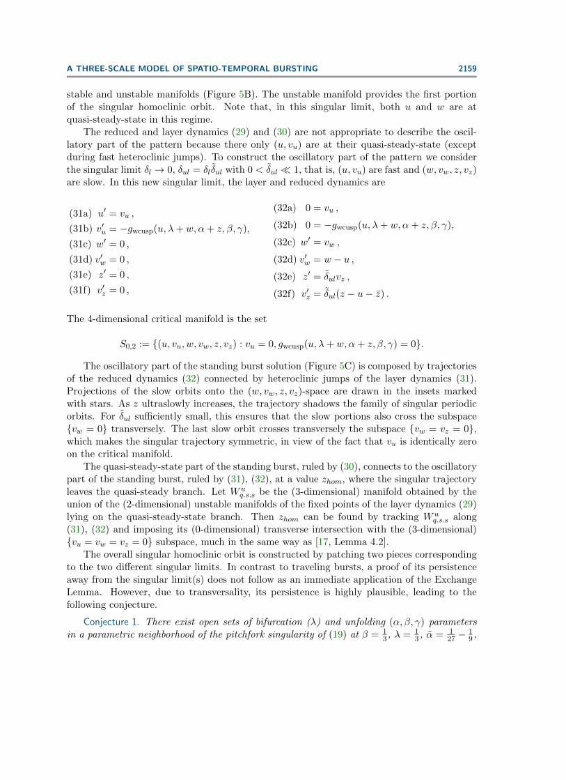
Figure 6. Parameters for traveling burst (left plot) are the same as in Figure 8. Parameters for travelingpulse (right plot) are the same as traveling bursts except λ = λPF (β) + 0.15 and α = αPF (β) + 0.4.

γ = 0 such that, for all parameters in those sets and almost all δul > 0 sufficiently small,the double singular limit (29)–(30), (31)–(32) possesses a transverse singular homoclinic orbitas sketched in Figure 5. Furthermore, model (5) possesses for δl > 0 sufficiently small ahomoclinic orbit near the transverse singular homoclinic orbit.

7. Modulation of spatio-temporal bursting. A main motivation in [11] to study a modelorganized by the winged-cusp singularity is that it provides a principled way to analyze the de-formation of bursting patterns as parameter paths in the universal unfolding of the singularity.The same geometric picture generalizes to spatio-temporal behaviors.

By changing the value of the bifurcation parameter λ and of the unfolding parameterα the traveling burst pattern predicted by Theorem 3 deforms to a classical traveling pulse(Figure 6). This is easily understood in terms of the geometry of the singular limit of theslow-fast subsystem. In particular, in the parameter region where there is no bistability in theslow-fast system, we recover the geometry of the FitzHugh–Nagumo model, as the ultraslowvariable barely affects the traveling pulse.

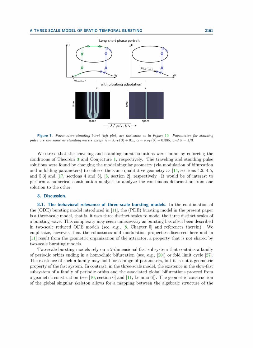
The same result holds for the deformation of standing bursts into standing pulses. Bychanging the value of the bifurcation parameter λ and of the unfolding parameters α and β,the standing burst pattern predicted by Conjecture 1 is changed into a classical standing pulse(Figure 7). Again, inspection of the geometry of the singular limit of the short-long rangesubsystem reveals the qualitative analogy with the geometry of the classical standing pulsesolution and the presence of the ultralong-range variable barely affects the standing pulsesolution.


(u ,u )rest rest

u

w

Long-short phase portrait

with ultralong adaptation

(u ,u )rest rest

u

w

space

tim

e

space

tim

e

λ ,α ,β

Figure 7. Parameters standing burst (left plot) are the same as in Figure 10. Parameters for standingpulse are the same as standing bursts except λ = λPF (β) + 0.1, α = αPF (β) + 0.385, and β = 1/3.

We stress that the traveling and standing bursts solutions were found by enforcing theconditions of Theorem 3 and Conjecture 1, respectively. The traveling and standing pulsesolutions were found by changing the model singular geometry (via modulation of bifurcationand unfolding parameters) to enforce the same qualitative geometry as [14, sections 4.2, 4.5,and 5.3] and [17, sections 4 and 5], [5, section 2], respectively. It would be of interest toperform a numerical continuation analysis to analyze the continuous deformation from onesolution to the other.

8. Discussion.

8.1. The behavioral relevance of three-scale bursting models. In the continuation ofthe (ODE) bursting model introduced in [11], the (PDE) bursting model in the present paperis a three-scale model, that is, it uses three distinct scales to model the three distinct scales ofa bursting wave. This complexity may seem unnecessary as bursting has often been describedin two-scale reduced ODE models (see, e.g., [8, Chapter 5] and references therein). Weemphasize, however, that the robustness and modulation properties discussed here and in[11] result from the geometric organization of the attractor, a property that is not shared bytwo-scale bursting models.

Two-scale bursting models rely on a 2-dimensional fast subsystem that contains a familyof periodic orbits ending in a homoclinic bifurcation (see, e.g., [20]) or fold limit cycle [27].The existence of such a family may hold for a range of parameters, but it is not a geometricproperty of the fast system. In contrast, in the three-scale model, the existence in the slow-fastsubsystem of a family of periodic orbits and the associated global bifurcations proceed froma geometric construction (see [10, section 6] and [11, Lemma 6]). The geometric constructionof the global singular skeleton allows for a mapping between the algebraic structure of the


universal unfolding of the organizing singularity and the observed dynamical behavior. Inother words, close to the three-time-scale singular limit, the observed dynamical behavior isfully determined by the algebraic property of the organizing center. Such a mapping does notexist in two-time-scale bursting models.

The mapping between the algebraic structure and the dynamical behavior is key to arigorous study of modulation of three-scale spatio-temporal patterns in terms of paths in theuniversal unfolding of the organizing singularity. The physiological relevance of this analysisin the purely temporal case is illustrated in [11, section 3] and [7]. We anticipate a similarpotential for the three scale model of the present paper in the analysis of spatio-temporalpattern formation.

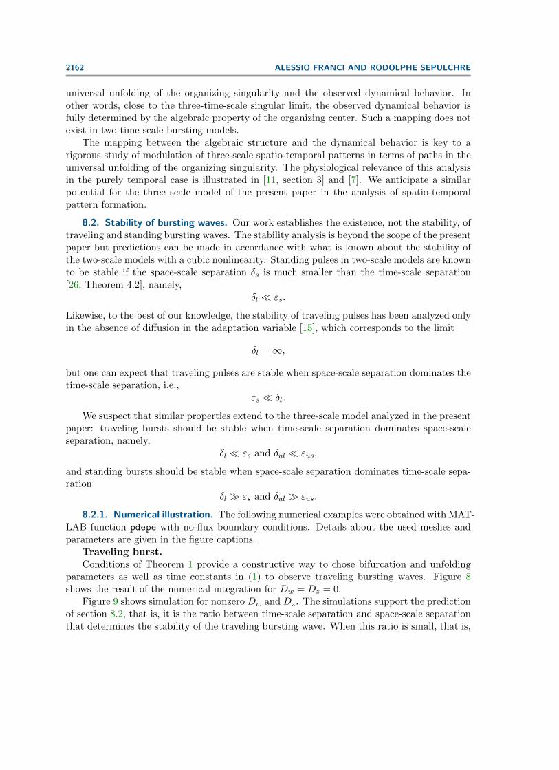
8.2. Stability of bursting waves. Our work establishes the existence, not the stability, oftraveling and standing bursting waves. The stability analysis is beyond the scope of the presentpaper but predictions can be made in accordance with what is known about the stability ofthe two-scale models with a cubic nonlinearity. Standing pulses in two-scale models are knownto be stable if the space-scale separation δs is much smaller than the time-scale separation[26, Theorem 4.2], namely,

δl � εs.

Likewise, to the best of our knowledge, the stability of traveling pulses has been analyzed onlyin the absence of diffusion in the adaptation variable [15], which corresponds to the limit

δl =∞,

but one can expect that traveling pulses are stable when space-scale separation dominates thetime-scale separation, i.e.,

εs � δl.

We suspect that similar properties extend to the three-scale model analyzed in the presentpaper: traveling bursts should be stable when time-scale separation dominates space-scaleseparation, namely,

δl � εs and δul � εus,

and standing bursts should be stable when space-scale separation dominates time-scale sepa-ration

δl � εs and δul � εus.

8.2.1. Numerical illustration. The following numerical examples were obtained with MAT-LAB function pdepe with no-flux boundary conditions. Details about the used meshes andparameters are given in the figure captions.

Traveling burst.Conditions of Theorem 1 provide a constructive way to chose bifurcation and unfolding

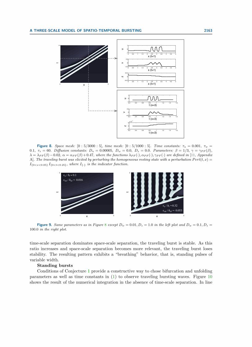
parameters as well as time constants in (1) to observe traveling bursting waves. Figure 8shows the result of the numerical integration for Dw = Dz = 0.

Figure 9 shows simulation for nonzero Dw and Dz. The simulations support the predictionof section 8.2, that is, it is the ratio between time-scale separation and space-scale separationthat determines the stability of the traveling bursting wave. When this ratio is small, that is,


0 0.5 1 1.5 2 2.5 3 3.5 4 4.5 5−1

0

1

x (t=1)

u

0 0.5 1 1.5 2 2.5 3 3.5 4 4.5 5−0.5

0

0.5

x (t=1)

v

0 0.5 1 1.5 2 2.5 3 3.5 4 4.5 5−0.01

0

0.01

x (t=1)

z

0.2 0.4 0.6 0.8 1 1.2 1.4 1.6−1

0

1

t (x=3)

u

0.2 0.4 0.6 0.8 1 1.2 1.4 1.6−0.5

0

0.5

t (x=3)

v

0.2 0.4 0.6 0.8 1 1.2 1.4 1.6−5

0

5x 10

−3

t (x=3)

z

0 5

1.5

x

t

Figure 8. Space mesh: [0 : 5/3000 : 5], time mesh: [0 : 5/1000 : 5]. Time constants: τu = 0.001, τw =0.1, τz = 60. Diffusion constants: Du = 0.00005, Dw = 0.0, Dz = 0.0. Parameters: β = 1/3, γ = γPF (β),λ = λPF (β)−0.02, α = αPF (β)+ 0.47, where the functions λPF (·), αPF (·), γPF (·) are defined in [11, AppendixA]. The traveling burst was elicited by perturbing the homogeneous resting state with a perturbation Pert(t, x) =I{0<x<0.05} I{0<t<0.25}, where I{·} is the indicator function.

0 5

2

x

t

0 5

2

x

t

εs / δl = 0.1

εus / δul ~ 0.016

εs / δl ~0.32

εus / δul ~ 0.053

Figure 9. Same parameters as in Figure 8 except Dw = 0.01, Dz = 1.0 in the left plot and Dw = 0.1, Dz =100.0 in the right plot.

time-scale separation dominates space-scale separation, the traveling burst is stable. As thisratio increases and space-scale separation becomes more relevant, the traveling burst losesstability. The resulting pattern exhibits a “breathing” behavior, that is, standing pulses ofvariable width.

Standing burstsConditions of Conjecture 1 provide a constructive way to chose bifurcation and unfolding

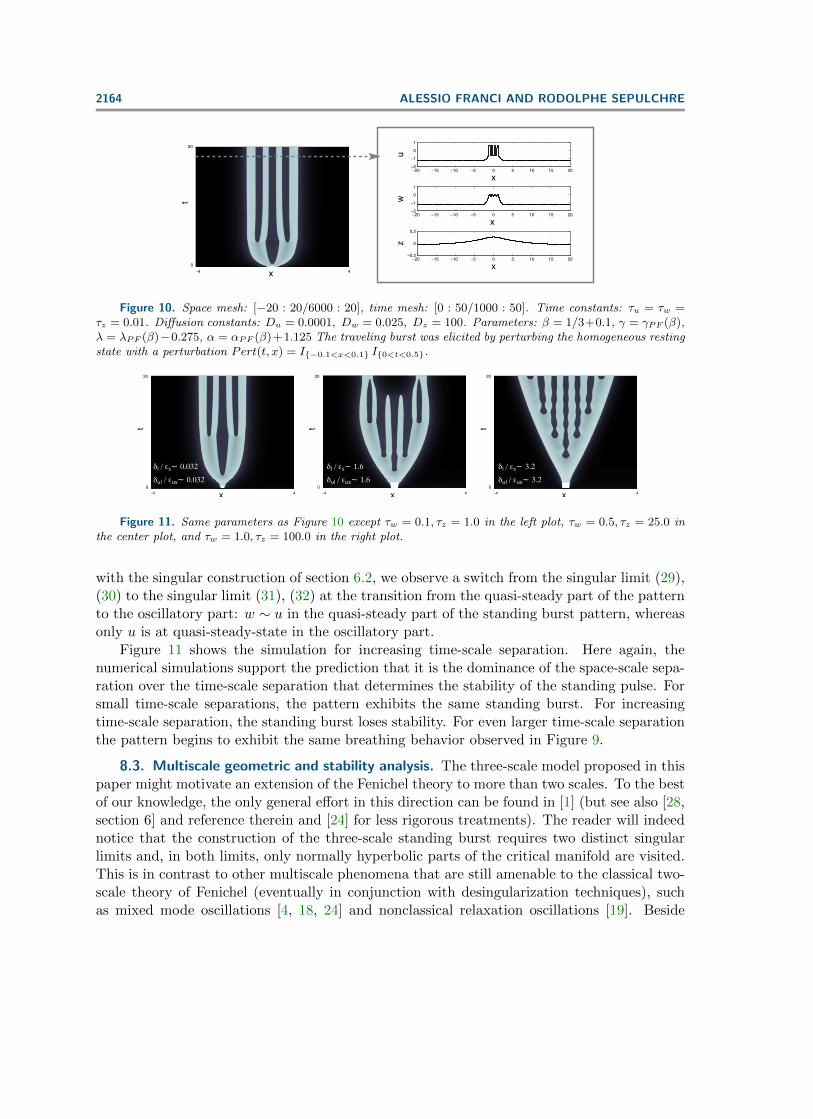
parameters as well as time constants in (1) to observe traveling bursting waves. Figure 10shows the result of the numerical integration in the absence of time-scale separation. In line


-4 4

50

x

t

0

−20 −15 −10 −5 0 5 10 15 20−2

−1

0

1

x

u

−20 −15 −10 −5 0 5 10 15 20−2

−1

0

1

x

w

−20 −15 −10 −5 0 5 10 15 20−0.2

0

0.2

x

z

Figure 10. Space mesh: [−20 : 20/6000 : 20], time mesh: [0 : 50/1000 : 50]. Time constants: τu = τw =τz = 0.01. Diffusion constants: Du = 0.0001, Dw = 0.025, Dz = 100. Parameters: β = 1/3+0.1, γ = γPF (β),λ = λPF (β)−0.275, α = αPF (β)+1.125 The traveling burst was elicited by perturbing the homogeneous restingstate with a perturbation Pert(t, x) = I{−0.1<x<0.1} I{0<t<0.5}.

-4 4

20

x

t

0

-4 4

20

x

t

0

-4 4

20

x

t0

δl / εs~ 0.032

δul / εus~ 0.032

δl / εs~ 1.6

δul / εus~ 1.6

δl / εs~ 3.2

δul / εus~ 3.2

Figure 11. Same parameters as Figure 10 except τw = 0.1, τz = 1.0 in the left plot, τw = 0.5, τz = 25.0 inthe center plot, and τw = 1.0, τz = 100.0 in the right plot.

with the singular construction of section 6.2, we observe a switch from the singular limit (29),(30) to the singular limit (31), (32) at the transition from the quasi-steady part of the patternto the oscillatory part: w ∼ u in the quasi-steady part of the standing burst pattern, whereasonly u is at quasi-steady-state in the oscillatory part.

Figure 11 shows the simulation for increasing time-scale separation. Here again, thenumerical simulations support the prediction that it is the dominance of the space-scale sepa-ration over the time-scale separation that determines the stability of the standing pulse. Forsmall time-scale separations, the pattern exhibits the same standing burst. For increasingtime-scale separation, the standing burst loses stability. For even larger time-scale separationthe pattern begins to exhibit the same breathing behavior observed in Figure 9.

8.3. Multiscale geometric and stability analysis. The three-scale model proposed in thispaper might motivate an extension of the Fenichel theory to more than two scales. To the bestof our knowledge, the only general effort in this direction can be found in [1] (but see also [28,section 6] and reference therein and [24] for less rigorous treatments). The reader will indeednotice that the construction of the three-scale standing burst requires two distinct singularlimits and, in both limits, only normally hyperbolic parts of the critical manifold are visited.This is in contrast to other multiscale phenomena that are still amenable to the classical two-scale theory of Fenichel (eventually in conjunction with desingularization techniques), suchas mixed mode oscillations [4, 18, 24] and nonclassical relaxation oscillations [19]. Beside


desingularization, the analysis in those reference is, in spirit, similar to the traveling burstanalysis of the present paper, in particular, in terms of conditions imposed on the time-scaleratios that allow us to reduce the analysis to a two-scale singularly perturbed dynamics.The extension of the Exchange Lemma to general multiscale singularly perturbed dynamicalsystems seems of particular relevance.

Also the problem of stability of the constructed multiscale spatio-temporal pattern shouldbe addressed carefully and more rigorously. The Evan’s function technique was successfullyapplied in the two-scale scenario both for traveling [15] and standing [17] pulses. An extensionto the three-scale scenario might be natural.

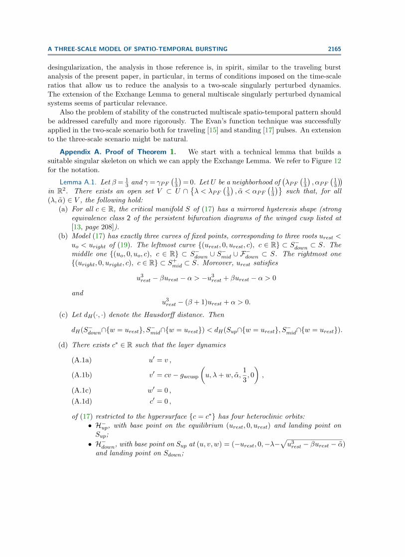
Appendix A. Proof of Theorem 1. We start with a technical lemma that builds asuitable singular skeleton on which we can apply the Exchange Lemma. We refer to Figure 12for the notation.

Lemma A.1. Let β = 13 and γ = γPF

(13

)= 0. Let U be a neighborhood of

(λPF

(13

), αPF

(13

))in R2. There exists an open set V ⊂ U ∩

{λ < λPF

(13

), α < αPF

(13

)}such that, for all

(λ, α) ∈ V , the following hold:(a) For all c ∈ R, the critical manifold S of (17) has a mirrored hysteresis shape (strong

equivalence class 2 of the persistent bifurcation diagrams of the winged cusp listed at[13, page 208]).

(b) Model (17) has exactly three curves of fixed points, corresponding to three roots urest <uo < uright of (19). The leftmost curve {(urest, 0, urest, c), c ∈ R} ⊂ S−down ⊂ S. Themiddle one {(uo, 0, uo, c), c ∈ R} ⊂ S−down ∪ S

−mid ∪ F

−down ⊂ S. The rightmost one

{(uright, 0, uright, c), c ∈ R} ⊂ S+mid ⊂ S. Moreover, urest satisfies

u3rest − βurest − α > −u3

rest + βurest − α > 0

andu3rest − (β + 1)urest + α > 0.

(c) Let dH(·, ·) denote the Hausdorff distance. Then

dH(S−down∩{w = urest}, S−mid∩{w = urest}) < dH(Sup∩{w = urest}, S−mid∩{w = urest}).

(d) There exists c∗ ∈ R such that the layer dynamics

u′ = v ,(A.1a)

v′ = cv − gwcusp

(u, λ+ w, α,

1

3, 0

),(A.1b)

w′ = 0 ,(A.1c)

c′ = 0 ,(A.1d)

of (17) restricted to the hypersurface {c = c∗} has four heteroclinic orbits:• H−up, with base point on the equilibrium (urest, 0, urest) and landing point onSup;

• H−down, with base point on Sup at (u, v, w) = (−urest, 0,−λ−√u3rest − βurest − α)

and landing point on Sdown;


λ=λPF(1/3)

~

~

L2

L > L1 2

α=αPF(1/3)

α<αPF(1/3)λ<λPF(1/3)

(u0,u0)

(urest,urest)

(uright,uright)

u

wvu

B)A)Sup

Fup Hup

Hup

Hdown

Sdown

Smid

L1

Fup

Hdown

SmidFdown

Sdown

~

~

Figure 12. Geometric construction of the singular phase portrait in Figure 3A. Left: critical manifoldand fixed points at the pitchfork singularity (gray) and for λ and α satisfying the conditions of Lemma A.1(black). Right: heteroclinic orbits of the layer dynamics and the different invariant manifolds involved in

their construction. F+/−down and F+/−

up denotes the fourfold singularities in the mirrored hysteresis persistent

bifurcation diagram. S+/−down, S

+/−mid , and Sup are the disconnected open submanifold of S, such that F+/−

down ∪F+/−up ∪ S+/−

mid ∪ Sup = S. L1 and L2 denote the distances dH(Sup ∩ {w = urest}, S−mid ∩ {w = urest}) anddH(S−down ∩ {w = urest}, S−mid ∩ {w = urest}), respectively.

• H+up and H+

down, which are obtained by symmetry of the layer dynamics withrespect to the hypersurface {w = −λ}.

Let Sup and S+down be compact, connected, normally hyperbolic submanifolds of Sup

and S+down, respectively, that contain all the base and landing points of the hetero-

clinic orbits. Then H−up is obtained as the transverse intersection (in the (u, v, w, c)space) of the 2-dimensional unstable manifold W u

rest of the curve of fixed points{(urest, 0, urest, c), c near c∗} with the 3-dimensional stable manifold W s(Sup). Theheteroclinic orbits H−down, H

+up, H+

down are obtained as the transverse intersection (inthe (u, v, w, c) space) of the 2-dimensional unstable manifold W u(Sbase|c=c∗) of the in-variant manifold Sbase containing the base points restricted to the hypersurface {c = c∗}with the 3-dimensional stable manifold W s(Sland) of the invariant manifold Sland con-taining the landing points.

Proof of Lemma A.1. Points (a), (b), and (c) follow from phase plane analysis (Figure12) quantitatively supported by the inspection of transition varieties and persistent bifurca-tion diagrams of the critical manifold (gwcusp(u, λ, α, β, γ) = 0) and fixed point (19) equa-tions of (17), both cubic universal unfolding of the winged cusp, near the singularity at(u, λ, α, β, γ) = (−1

3 ,13 ,−

227 ,

13 , 0). This singularity is transcritical for the critical manifold

equation and pitchfork for the fixed point equation. For the algebraic expressions of the tran-sition and bifurcation varieties, see [13, p. 206] for the critical manifold equation and [11] forthe fixed point equation.

To prove (d) we use existing results on the FitzHugh–Nagumo traveling pulse equation[14, sections 4.2 and 5.3]. Points (a)–(c) imply that there exists a diagonal diffeomorphismfrom a neighborhood of the hypersurface {w = urest} to a neighborhood of the hypersurface{w = 0}, which is the identity on v and is affine in u, and which maps the layer dynamics(A.1) to the layer dynamics of the FitzHugh–Nagumo traveling pulse equation [14, (4.2)] with


parameter 0 < a < 1/2 given by

a =dH(S−down ∩ {w = urest}, S−mid ∩ {w = urest})dH(Sup ∩ {w = urest}, S−down ∩ {w = urest})

.

Explicitly, the diffeomorphism is given by

(A.2)

uvwc

7→

Cu+ urestv

−√w − u3

rest + βurest − α− λc

,

where C is a scaling factor such that u = 1 is the largest of the three roots of the transformedlayer dynamics fixed point equation computed at w = 0, that is, −(Cu + urest)

3 + 13(Cu +

urest) − (urest + λ)2 − α = 0. The smallest root is by construction at u = 0 and, by (c),the middle root is u = a with 0 < a < 1/2. Because by (b) −u3

rest + βurest − α > 0, thediffeomorphism is well defined.

We now invoke the fact that (A.2) is diagonal, its affine dependence on u, and the fact thatit is the identity on v and c. By the chain rule, these properties imply that the differentialforms that we use to track invariant manifolds of (A.1) and their intersections are givenby linear scaling of the same computations as in the classical FitzHugh–Nagumo equation[14, section 4.5]. As for the classical FitzHugh–Nagumo equation, we conclude the existenceof c∗ 6= 0 such that (A.1) possesses for c = c∗ the heteroclinic orbit H−up satisfying thetransversality conditions of point (d).

Existence of the heteroclinic orbits H−down, H+up, and H+

down, and their transversality prop-erties follow again from local equivalence of (A.1) with the layer dynamics of the FitzHugh–Nagumo traveling pulse equation [14, (4.2)] and by following the same construction as in [14,section 5.3].

To prove the theorem, we track the 2-dimensional unstable manifold W urest of the curve

of fixed points {(urest, 0, urest, c), c near c∗}, that is, we follow the mapping of a germ ofW urest through the flow associated with (17). For εs > 0 and sufficiently small, let Sup,εs and

S+down,εs

be the slow manifolds obtained as Fenichel perturbations of Sup and S+down, respec-

tively. Thanks to Lemma A.1(d), we can apply [16, Lemma 4.1] and the Exchange Lemma andfollow the same arguments as the last two paragraphs of the proof of the Theorem in [16, sec-tion 4] to conclude the following: W u

rest intersects W s(Sup,εs) transversely along H−up; between

H−up and H+down it lies O(εs)-close to Sup. It leaves Sup along H+

down intersecting W s(S+down,εs

)

transversely. Between H+down and H+

up it lies O(εs)-close to S+down; finally, it leaves S+

down

along H+up, again, intersecting W s(Sup,εs) transversely. We can continue to track the for-

ward mapping of W urest through the flow associated with (17) to conclude that it intersects

W s(Sup,εs) and W s(S+down,εs

) transversely infinitely many times. Since c is a parameter, all the(1-dimensional) transverse intersections are in the same {c = c}-slice for some c = c∗+O(εs).We claim that the trajectory containing all the transverse intersections, call it hεs , is theheteroclinic trajectory corresponding to the traveling front.

It remains to show that, in the same {c = c}-slice, there also exists a periodic solution `εsof (17) and that hεs ⊂ W s(`εs). To this aim, we track the 2-dimensional unstable manifold


W u(Sup,εs |c=c). By the Exchange Lemma, W u(Sup,εs |c=c) and W urest are O(εs)-C

1 close toeach other at the heteroclinic jump H+

down. It follows that, for εs sufficiently small, alsoW u(Sup,εs |c=c) comes back (under the flow associated with (17)) in a neighborhood of Suptransversely intersecting W s(Sup,ε) inside {c = c}. It follows that the 1-dimensional transverse(in the (u, v, w, c) space) intersection W u(Sup,εs |c=c)∩T W s(Sup,εs) defines a periodic orbit `εsof (17) in the slice c = c. Because W s(`εs) = W s(Sup,εs |c=c) and hεs ⊂ W s(Sup,εs |c=c), thestatement is proved for β = 1/3 and γ = 0. For β 6= 1/3, γ 6= 0, the theorem follows fromthe persistence of all the transverse intersections used in the construction to arbitrary C1

perturbations.

Appendix B. Proof of Theorem 2. We use two technical lemmas to build a suitablesingular skeleton on which we can apply the Exchange Lemma.

Lemma B.1. Let β = 13 and γ = γPF (1

3) = 0. For all α ∈ [αPF (1/3), 0) and all λ ∈ R, thelayer dynamics of (18),

u′ = vu ,(B.1a)

v′u = −gwcusp

(u, λ+ w, α,

1

3, 0

),(B.1b)

possess two heteroclinic orbits at w = wh1(α) and two heteroclinic orbits at w = wh2(α) withwh1(α) = −λ −

√−α < −λ < −λ +

√−α = wh2(α). For α = 0, model (B.1) possesses two

heteroclinic orbits at w = −λ.

Proof of Lemma B.1. For w = wh1(α) or w = wh2(α), (B.1) reduces to

u′ = vu ,

v′u = −u3 +u

3,

which is Hamiltonian, has three fixed point at vu = 0 and u = − 1√3, 0, 1√

3, and satisfies

∫ 1√3

− 1√3

(−u3 +

u

3

)du = 0.

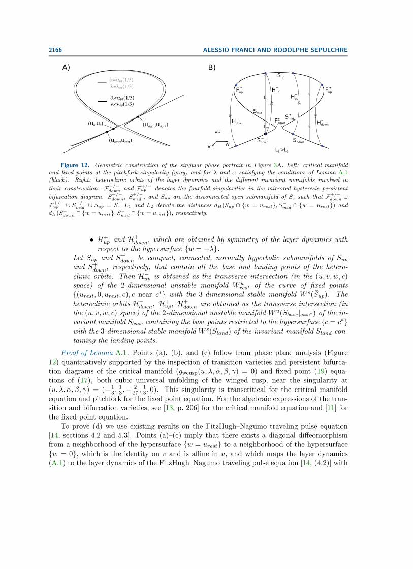
The notation in the next lemma is defined in Figure 13.

Lemma B.2. Let β = 13 and γ = γPF (1

3) = 0. There exist a neighborhood U of (λ, α) =

(1/√

3, 0) and an open set V ⊂ U ∩ {λ < 1/√

3, α < 0}, such that, for all (λ, α) ∈ V thefollowing hold:

(a) The critical manifold of model (18) belongs to class 3 of the persistent bifurcationdiagrams of the winged cusp [13, p. 208]. Let wfold be the w-coordinate of the rightfold of the critical manifold. Let u = udown(w) be the function such that the lowerbranch of the critical manifold C− = {(u, vu, w, vw) = (udown(w), 0, w, 0)} and uup(w)the function such that the upper branch of the critical manifold between the two foldsingularities C+ = {(u, vu, w, vw) = (uup(w), 0, w, 0)}.

(b) Model (18) has a unique fixed point at (wrest, 0, wrest, 0) with wrest < −λ.


λ=1/31/2

~

~

α=0

α<0λ<1/31/2

(wrest,wrest)

B)A)

-λwh1 wh2

wh1 wh2wrest

C+

wvw

u

vw,h1vw,h2

-vw,h2-vw,h1

C-

(umax,0,wmax,0)

~

~

Figure 13. Geometric construction of the singular phase portrait in Figure 3B.

(c) The following inequalities hold:∫ wh1

wrest

(udown(s)− s

)ds+

∫ wfold

wh1

(uup(s)− s

)ds > 0 ,(B.2a) ∫ wh1

wrest

(udown(s)− s

)ds+

∫ wh2

wh1

(uup(s)− s

)ds < 0 .(B.2b)

Proof of Lemma B.2. Points (a), (b) follow from phase plane analysis (Figure 13) quan-titatively supported by the inspection of transition varieties and persistent bifurcation dia-grams of the critical manifold (gwcusp(u, λ, α, β, γ) = 0) and fixed point (19) equations of (17),both cubic universal unfolding of the winged cusp, near the singularity at (u, λ, α, β, γ) =(xPF (1

3), λPF (13), αPF (1

3), 1/3, γPF (13)) = (−1

3 ,13 ,−

227 ,

13 , 0). This singularity is transcritical

for the critical manifold equation and pitchfork for the fixed point equation. For the algebraicexpressions of the transition and bifurcation varieties; see [13, p. 206] for the critical manifoldequation and [11] for the fixed point equation.

Point (c). Because∫ wfoldwh1

(uup(s) − s)ds > 0 and wrest = wh1 for (λ, α) = (1/√

3, 0), it

follows that (B.2a) is satisfied for (λ, α) = (1/√

3, 0). By continuity of the integral operator,the same holds true for (λ, α) sufficiently close to (1/

√3, 0).

To prove the second inequality, observe that∫ wh1wrest

(udown(s)− s)ds < 0 and wh1 = wh2 for

λ < 1/√

3 and α = 0. Therefore (B.2b) is satisfied for λ < 1/√

3 and α = 0. By continuity,the same holds for (λ, α) sufficiently close to (1/

√3, 0).

The existence of the homoclinic orbit now follow exactly as [17, sections 4 and 5]. The twomodels indeed share the exact same geometry (compare Figure 13 right and [17, Figure 4]).The sole difference is the absence of a fixed point on C+. This only changes the constructionof the slow portion of the singular homoclinic orbit on C+. Construction of this portion herefollows the same line as in [5, pp. 238 and 239].

The same construction is used for the periodic orbit. The only difference is that the initialslow portion is now defined as the slow trajectory passing through the point (wh2 , vw,h2)


instead as the unstable manifold of the fixed point. Then, all the results of [17, sections 4 and5] still hold.

The fact that the homoclinic and singular periodic orbits are O(δl)-close to each other nearthe point (umax, 0, wmax, 0), where w reaches its maximum along the homoclinic trajectoryfollows from the fact that, near C+, the homoclinic and the periodic orbits are perturbationsof, and henceO(δl)-close to, the same invariant manifold; likewise, for their stable and unstablemanifolds.

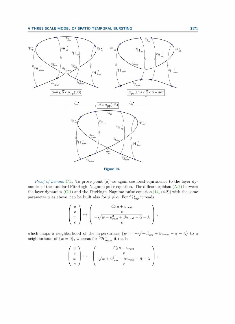
Appendix C. Proof of Theorem 3. We refer the reader to Figure 14 for the notationused in the following lemma.

Lemma C.1. Let β = 13 and γ = γPF (1

3) = 0. Let V ⊂ R2 and c∗ 6= 0 be defined as in thestatement of Lemma A.1. For all (λ, α) ∈ V , the following hold true:

(a) There exists ∆α∗ > 0 and δ > 0 such that, for all α ∈ [α−δ,∆α∗), the layer dynamics

u′ = v ,(C.1a)

v′ = cv − gwcusp

(u, λ+ w, α,

1

3, 0

),(C.1b)

w′ = 0 ,(C.1c)

c′ = 0(C.1d)

of (17) restricted to the hypersurface {c = c∗} has four heteroclinic orbits αH+/−up/down

that are all obtained as the transverse intersections (in the (u, v, w, c) space) of the 2-dimensional unstable manifold W u(αSbase|c=c∗) of the invariant manifold αSbase, wherethe base point lies restricted to the hypersurface {c = c∗} with the 3-dimensional stablemanifold W s(αSland) of the invariant manifold αSland where the landing point lies.2

(b) For α = α+ ∆α∗ the two heteroclinic orbits αH+/−up merge in a fast heteroclinic jump

H0up. This heteroclinic lies in the hypersurface {w = −λ} and is obtained as the

nontransverse intersection W u(αSdown|c=c∗) ∩W s(αSup).

(c) The two downward heteroclinic jumps αH+/−down persist for α ∈ [α+ ∆α∗, α+ ∆α∗ + δ)

and with the same transversality properties as in (a).(d) For all α ∈ [α, α + ∆α∗), let αwup <α wdown be the w-coordinate of the hetero-

clinic αH+up and αH+

down, respectively. There exists C > 0 such that, for all α ∈[α, αPF (1/3)],∫ αwdown

αwup

(u|αS+down− (α− α))dw +

∫ αwdown

αwup

(u|αSup − (α− α))dw > C

and, for all α ∈ (αPF (1/3), α+ ∆α∗),∫ αwdown

αwup

(u|αSdown − (α− α))dw +

∫ αwdown

αwup

(u|αSup − (α− α))dw > C.

2As in Lemma A.1, the overline means a compact, connected, normally hyperbolic submanifold of therelative manifold that contains all the base and landing points of the heteroclinic orbits.


αSdown

αSmidαSmid

αSdown

αSup

αF down

αF upupαF αHup

αH up

αHdown

αH down

~

~

~

~

~

~

~

~

~

~

~

~

αSdown

αSmid

αSup

αF upupαF αHup

αH up

αHdown

αH down

~

~

~

~

~

~

~

~

~

αSdown

αSmid

αSmid

αSdown

αSup

αF upup

αF αHup

αH up

αHdown

αH down

~

~

~

~

~

~

~

~

~

~

~

TC

α−δ < α < α (1/3)~PF α (1/3) < α < α + Δα∗~

PF

α = α (1/3)~PF

α~ α~

Figure 14.

Proof of Lemma C.1. To prove point (a) we again use local equivalence to the layer dy-namics of the standard FitzHugh–Nagumo pulse equation. The diffeomorphism (A.2) betweenthe layer dynamics (C.1) and the FitzHugh–Nagumo pulse equation [14, (4.2)] with the sameparameter a as above, can be built also for α 6= α. For αH−up it reads

uvwc

7→

Cαu+ urestv

−√w − u3

rest + βurest − α− λc

,

which maps a neighborhood of the hypersurface {w = −√−u3

rest + βurest − α − λ} to aneighborhood of {w = 0}, whereas for αH−down it reads

uvwc

7→ −

Cαu− urestv√

w + u3rest − βurest − α− λ

c

,


which maps a neighborhood of the hypersurface {w = −√u3rest − βurest − α− λ} to a neigh-

borhood of {w = 0}. For αH+up/down we use symmetry with respect to the hypersurface

{w = −λ}. The w-coordinate of the heteroclinics αH−up and αH−down are given by αw−up =

−√−u3

rest + βurest − α − λ and αw−down = −√u3rest − βurest − α − λ, respectively. Their

mirrors with respect to the hypersurface {w = −λ} are αw+up =

√−u3

rest + βurest − α − λand αw−down =

√u3rest − βurest − α − λ. Existence of the four heteroclinic orbits and their

transversality conditions then follows as in [14, section 5.3].The value ∆α∗ of point (b) is computed by imposing −u3

rest + βurest − α−∆α∗ = 0. Asα→ α + ∆α∗, the two heteroclinics αH−up and αH−up converge to each other in the Hausdorff

distance, because limα→α+∆α∗αw−up = limα→α+∆α∗

αw+up = −λ. For α = α+ ∆α∗, the map

uv−λc

7→

Cu+ urestv0c

maps the layer dynamics (C.1) restricted to the hypersurface {w = −λ} to the traveling waveproblem [14, (4.10)] with the same parameter a as above. With the same computation as[14, section 4.5], we conclude the existence of the heteroclinic H0

up in the same hypersurface

{c = c∗} as αH+/−up/down, α ∈ [α, α + ∆α). The nontransversality condition follows by the

fact that transversality is not compatible with a (local) change in the number of transverseintersections.

By Lemma A.1(b), we have u3rest−βurest > −u3

rest +βurest. This in turn implies that the

outer heteroclinics H+/−down persist and with the same properties as in (a) for α = α+ ∆α∗ and,

by continuity, also for α+ ∆α∗ < α < α+ ∆α∗ + δ, which proves (c).To prove point (d), we start by noticing that, by antysimmetry in u of the layer dynamics

(A.1), for all α ∈ [α, αPF (13)],∫ αwdown

αwup

u|αS+down

dw = −∫ αwdown

αwup

u|αSupdw

and, for all α ∈ (αPF (13), α+ ∆α∗),∫ αwdown

αwup

u|αSdowndw = −∫ αwdown

αwup

u|αSupdw.

The proof of (d) therefore reduces to showing that −urest−(α−α) > 0 for all α ∈ [α, α+∆α∗).It suffices to prove this for α = α + ∆α∗. By (b), ∆α∗ = −u3

rest + βurest − α, so we have toprove that u3

rest − (β + 1)urest + α > 0, which was proved in Lemma A.1(b).

A straightforward corollary of Lemma C.1, obtained by replacing α by α + z, is thatthe singular (εs = 0) phase portrait of (6) is as depicted in Figure 4. Let T denote the(2-dimensional) critical manifold of (6). Slices zT ⊂ T at z ∈ [zrest − δ, z∗ + δ] are given byembedding in R5 the critical manifold of (C.1) for α = α + z. For each z ∈ [zrest − δ, z∗ + δ]


we denote with zT+/−down/up the embedding of αS

+/−up/down, α = α + z, defined as in Figure 14

and, similarly, with zT+/−down/up the embedding of αS

+/−up/down. For each z ∈ [zrest − δ, z∗ + δ] we

denote with zH+/−up/down and zH0

up the embedding of αH+/−up/down and αH0

up, where they exist.

This singular phase portrait provides a skeleton for the application of the theorem in [16,section 4]. In particular, we can build a singular homoclinic trajectory from the resting point

to itself consisting of finitely many jumps along the family of heteroclinic orbits zH+/−up/down

of the layer dynamics of (26) connected slow trajectories of the reduced dynamics (27). This

trajectory was sketched in Figure 4. Transversality properties of αH+/−up/down will translate into

the needed transversality condition [16, (4.2) and (4.3)].For the existence of the singular homoclinic trajectory, we invoke Lemma C.1(d). It implies

that for εus > 0 and as long as z < z∗, the z-coordinate of two successive jumps down and oftwo successive jumps up is strictly uniformly monotonically increasing by an amount boundedfrom below by Cεus. After the last jump down the trajectory might cross the hypersurface{w = −λ} at z = z∗, which would break the transversality required by the Exchange Lemma.However, by smooth dependence of trajectories on the model parameters [21, Theorem D.5],this behavior is not generic in εus > 0, which explains the genericity condition in the statementof the theorem. The trajectory then converges toward the quasi-steady-state of the slow-fastsubsystem (6a)–(6c) and then to rest.

We now verify the two transversality conditions [16, (4.2) and (4.3)]. Let

T 0 :=⋃

z∈[−δ,αPF ( 13

)−α]

(zT−down ∪zT+

down) ∪⋃

z∈(αPF ( 13

)−α,∆α∗+δ]

zTdown

and

T 1 :=z⋃

z∈[−δ,∆α∗+δ]

Tup,

that is, T 0 and T 1 are compact, connected, normally hyperbolic (for the layer dynamics (26))submanifolds of the critical manifold T that contains all the base and landing points of the

heteroclinic orbits zH+/−up/down, in particular, T 0 contains base points of upward heteroclinic

and landing points of downward heteroclinic, and vice versa for T 1.To verify [16, (4.2)], we have to prove that, in the layer dynamics (26), the first hetero-

clinic jump of the singular homoclinic trajectory, along zrestH−up, is obtained as the transverseintersection W u

rest ∩T W s(T 1), where W urest is the 2-dimensional unstable manifold of the line

of fixed points {(urest, 0, urest, c, 0), c near c∗}, whereas W s(T 1) is 4-dimensional. Note thatW urest ⊂ {z = zrest} and that W s(T 1) ∩ {z = zrest} = W s(Sup), where Sup is defined as in

Lemma A.1. It follows by Lemma A.1(d) that W urest ∩T W s(T 1) inside {z = zrest}. Since the

full space only adds the z-direction, W urest ∩T W s(T 1), which verifies [16, (4.2)] for (6).

Next, we verify [16, (4.3)] for all successive jumps. We write the condition explicitly forthe first jump down along zH+

down for some z > zrest. Computations for other jumps aresimilar and therefore omitted. We have to verify that W u(T 1|sing.orbit) ∩T W s(T 0). First,we note that the singular homoclininc trajectory is in the hypersurface {c = c∗}. Second,as εus → 0, the slow motion after the first jump up converges in the Hausdorff distance


to the hypersurface {z = zrest}, that is, limεus→0 T1|sing.orbit = T 1|c=c∗,z=zrest , where the

limit is again in the Hausdorff distance. Since W u(T 1|c=c∗,z=zrest) ⊂ {z = zrest}, reasoningas above we can invoke Lemma A.1(d) to conclude that W u(T 1|c=c∗,z=0) ∩T W s(T 0) insidethe subspace {z = zrest} and, therefore, by adding the z-dimension, in the whole space.Because W u(T 1|sing.orbit) is also O(εus)-close to W u(T 1|c=c∗,z=zrest) for εus sufficiently small,also W u(T 1|sing.orbit) ∩T W s(T 0).

We can now apply the theorem in [16, section 4] to conclude that, for εs > 0 sufficientlysmall, there exists a unique homoclinic solution of (6), which proves the statement of thetheorem for β = 1/3 and γ = 0. For β 6= 1/3 and γ 6= 0, the statement follows from thepersistence of transverse intersections to arbitrary C1 perturbations. �

REFERENCES

[1] P. Cardin, P. da Silva, and M. Teixeira, Three time scale singular perturbation problems and nons-mooth dynamical systems, Quart. Appl. Math., 72 (2014), pp. 673–687.

[2] G. A. Carpenter, A geometric approach to singular perturbation problems with applications to nerveimpulse equations, J. Differential Equations, 23 (1977), pp. 335–367.

[3] P. Carter and B. Sandstede, Fast pulses with oscillatory tails in the Fitzhugh–Nagumo system, SIAMJ. Math. Anal., 47 (2015), pp. 3393–3441.

[4] M. Desroches, J. Guckenheimer, B. Krauskopf, C. Kuehn, H. M. Osinga, and M. Wechsel-berger, Mixed-mode oscillations with multiple time scales, SIAM Rev., 54 (2012), pp. 211–288.

[5] J. D. Dockery, Existence of standing pulse solutions for an excitable activator-inhibitory system, J.Dynam. Differential Equations, 4 (1992), pp. 231–257.

[6] A. Doelman, P. Van Heijster, and T. J. Kaper, Pulse dynamics in a three-component system:Existence analysis, J. Dynam. Differential Equations, 21 (2009), pp. 73–115.

[7] G. Drion, A. Franci, R. Dethier, and J. Sepulchre, Dynamic input conductances shape neuronalspiking, Eneuro, 2 (2015), e0031, doi:10.1523/ENEURO.0031-14.2015.

[8] G. B. Ermentrout and D. H. Terman, Mathematical Foundations of Neuroscience, Interdiscip. Appl.Math. 35, Springer, New York, 2010.

[9] R. FitzHugh, Impulses and physiological states in theoretical models of nerve membrane, Biophys. J., 1(1961), pp. 445–466.

[10] A. Franci, G. Drion, and R. Sepulchre, An organizing center in a planar model of neuronal excitabil-ity, SIAM J. Appl. Dyn. Syst., 11 (2012), pp. 1698–1722.

[11] A. Franci, G. Drion, and R. Sepulchre, Modeling the modulation of neuronal bursting: A singularitytheory approach, SIAM J. Appl. Dyn. Syst., 13 (2014), pp. 798–829.

[12] D. Golomb and Y. Amitai, Propagating neuronal discharges in neocortical slices: Computational andexperimental study, J. Neurophys., 78 (1997), pp. 1199–1211.

[13] M. Golubitsky and D. G. Schaeffer, Singularities and groups in bifurcation theory, Appl. Math. Sci.51, Springer, New York, 1985.

[14] C. Jones, Geometric singular perturbation theory, in Dynamical Systems, Springer Lecture Notes inMath. 1609, Springer, Berlin, 1995, pp. 44–120.

[15] C. K. R. T. Jones, Stability of the travelling wave solution of the Fitzhugh-Nagumo system, Trans. Amer.Math. Soc., 286 (1984), pp. 431–469.

[16] C. K. R. T. Jones and N. Kopell, Tracking invariant manifolds with differential forms in singularlyperturbed systems, J. Differential Equations, 108 (1994), pp. 64–88.

[17] C. K. R. T. Jones and J. E. Rubin, Existence of standing pulse solutions to an inhomogeneous reaction–diffusion system, J. Dynam. Differential Equations, 10 (1998), pp. 1–35.

[18] M. Krupa, N. Popovic, and N. Kopell, Mixed-mode oscillations in three time-scale systems: A pro-totypical example, SIAM J. Appl. Dyn. Syst., 7 (2008), pp. 361–420.

[19] C. Kuehn and P. Szmolyan, Multiscale geometry of the Olsen model and non-classical relaxation oscil-lations, J. Nonlinear Sci., 25 (2015), pp. 583–629.

http://dx.doi.org/10.1523/ENEURO.0031-14.2015


[20] E. Lee and D. Terman, Uniqueness and stability of periodic bursting solutions, J. Differential Equations,158 (1999), pp. 48–78.

[21] J. M. Lee, Introduction to Smooth Manifolds, 2nd ed., Grad. Texts In Math., Springer, New York, 2013.[22] D. Linaro, A. Champneys, M. Desroches, and M. Storace, Codimension-two homoclinic bifurca-

tions underlying spike adding in the Hindmarsh–Rose burster, SIAM J. Appl. Dyn. Syst., 11 (2012),pp. 939–962.

[23] E. Maeda, H. P. Robinson, and A. Kawana, The mechanisms of generation and propagation ofsynchronized bursting in developing networks of cortical neurons, J. Neurosci., 15 (1995), pp. 6834–6845.

[24] P. Nan, Y. Wang, V. Kirk, and J. E. Rubin, Understanding and distinguishing three-time-scaleoscillations: Case study in a coupled Morris–Lecar system, SIAM J. Appl. Dyn. Syst., 14 (2015),pp. 1518–1557.

[25] S. A. Newman and H. L. Frisch, Dynamics of skeletal pattern formation in developing chick limb,Science, 205 (1979), pp. 662–668.

[26] J. E. Rubin, Stability, bifurcations and edge oscillations in standing pulse solutions to an inhomogeneousreaction-diffusion system, Proc. Roy. Soc. Edinburgh Sect. A, 129 (1999), pp. 1033–1079.

[27] J. Su, J. Rubin, and D. Terman, Effects of noise on elliptic bursters, Nonlinearity, 17 (2003), pp. 133–157.

[28] T. Vo, R. Bertram, and M. Wechselberger, Multiple geometric viewpoints of mixed mode dynamicsassociated with pseudo-plateau bursting, SIAM J. Appl. Dyn. Syst., 12 (2013), pp. 789–830.

Documents

A Three-Scale Model of Spatio-Temporal Bursting