A Time-dependent SIR model for COVID-19 with Undetectable

THE LATEST VERSION WILL BE PLACED ON HTTP://GIBBS1.EE.NTHU.EDU.TW/A TIME DEPENDENT SIR MODEL FOR COVID 19.PDF 1

A Time-dependent SIR model for COVID-19 withUndetectable Infected Persons

Yi-Cheng Chen∗, Ping-En Lu†, Graduate Student Member, IEEE, Cheng-Shang Chang‡, Fellow, IEEE, andTzu-Hsuan Liu§

Institute of Communications EngineeringNational Tsing Hua UniversityHsinchu 30013, Taiwan, R.O.C.

Email: ∗[email protected], †[email protected], ‡[email protected],§[email protected]

The latest version will be placed on this link:http://gibbs1.ee.nthu.edu.tw/A TIME DEPENDENT SIR MODEL FOR COVID 19.PDF

Abstract—In this paper, we conduct mathematical and nu-merical analyses to address the following important questionsfor COVID-19: (Q1) Is it possible to contain COVID-19? (Q2)If COVID-19 can be contained, when will be the peak of theepidemic, and when will it end? (Q3) How do the asymptomaticinfections affect the spread of disease? (Q4) If COVID-19 cannotbe contained, what is the ratio of the population that needs to beinfected in order to achieve herd immunity? (Q5) How effectiveare the social distancing approaches? (Q6) If COVID-19 cannotbe contained, what is the ratio of the population infected inthe long run? For (Q1) and (Q2), we propose a time-dependentsusceptible-infected-recovered (SIR) model that tracks two timeseries: (i) the transmission rate at time t and (ii) the recoveringrate at time t. Such an approach is not only more adaptive thantraditional static SIR models, but also more robust than directestimation methods. Using the data provided by the NationalHealth Commission of the People’s Republic of China (NHC) [1],we show that the one-day prediction errors for the numbers ofconfirmed cases are almost less than 3%. Also, the turning point,defined as the day that the transmission rate is less than therecovering rate, is predicted to be Feb. 17, 2020. After that day,the basic reproduction number, known as the R0 value at time t,is less than 1. In that case, the total number of confirmed cases ispredicted to be around 80, 000 cases in China under our model.For (Q3), we extend our SIR model by considering two types ofinfected persons: detectable infected persons and undetectableinfected persons. Whether there is an outbreak in such a modelis characterized by the spectral radius of a 2× 2 matrix that isclosely related to the basic reproduction number R0. We plot thephase transition diagram of an outbreak and show that there areseveral countries, including South Korea, Italy, and Iran, that areon the verge of COVID-19 outbreaks on Mar. 2, 2020. For (Q4),we show that herd immunity can be achieved after at least 1− 1

R0fraction of individuals being infected and recovered from COVID-19. For (Q5) and (Q6), we analyze the independent cascade (IC)model for disease propagation in a random network specified bya degree distribution. By relating the propagation probabilitiesin the IC model to the transmission rates and recovering ratesin the SIR model, we show two approaches of social distancingthat can lead to a reduction of R0.

Index Terms—COVID-19, SARS-CoV-2, 2019-nCoV, Coron-avirus, Time-dependent SIR model, asymptomatic infection, herdimmunity, superspreader, independent cascade, social distancing.

I. INTRODUCTION

At the beginning of December 2019, the first COVID-19victim was diagnosed with the coronavirus in Wuhan, China.In the following weeks, the disease spread widely in Chinamainland and other countries, which causes global panic.The virus has been named “SARS-CoV-2,” and the disease itcauses has been named “coronavirus disease 2019 (abbreviated“COVID-19”). There have been 80, 151 people infected by thedisease and 2, 943 deaths until Mar. 2, 2020 according to theofficial statement by the Chinese government. To block thespread of the virus, there are some strategies such as city-wide lockdown, traffic halt, community management, socialdistancing, and propaganda of health education knowledge thathave been adopted by the governments of China and othercountries in the world.

Unlike the Severe Acute Respiratory Syndrome (SARS)and other infectious diseases, one problematic characteristicof COVID-19 is that there are asymptomatic infections (whohave very mild symptoms). Those asymptomatic infections areunaware of their contagious ability, and thus get more peopleinfected. The transmission rate can increase dramatically inthis circumstance. According to the recent report from WHO[2], only 87.9% of COVID-19 patients have a fever, and 67.7%of them have a dry cough. If we use body temperature as ameans to detect COVID-19 infected cases, then more than 10%of infected persons cannot be detected.

Due to the recent development of the epidemic, we areinterested in addressing the following important questions forCOVID-19:

(Q1) Is it possible to contain COVID-19? Are the com-monly used measures, such as city-wide lockdown,traffic halt, community management, and propagandaof health education knowledge, effective in contain-ing COVID-19?

(Q2) If COVID-19 can be contained, when will be thepeak of the epidemic, and when will it end?

(Q3) How do the asymptomatic infections affect thespread of disease?

HTTP://GIBBS1.EE.NTHU.EDU.TW/A_TIME_DEPENDENT_SIR_MODEL_FOR_COVID_19.PDF

http://gibbs1.ee.nthu.edu.tw/A_TIME_DEPENDENT_SIR_MODEL_FOR_COVID_19.PDF


(Q4) If COVID-19 cannot be contained, what is the ratioof the population that needs to be infected in orderto achieve herd immunity?

(Q5) How effective are the social distancing approaches,such as reduction of interpersonal contacts and can-celing mass gatherings in controlling COVID-19?

(Q6) If COVID-19 cannot be contained, what is the ratioof the population infected in the long run?

For (Q1), we analyze the cases in China and aim to predicthow the virus spreads in this paper. Specifically, we proposeusing a time-dependent susceptible-infected-recovered (SIR)model to analyze and predict the number of infected personsand the number of recovered persons (including deaths). In thetraditional SIR model, it has two time-invariant variables: thetransmission rate β and the recovering rate γ. The transmissionrate β means that each individual has on average β contactswith randomly chosen others per unit time. On the other hand,the recovering rate γ indicates that individuals in the infectedstate get recovered or die at a fixed average rate γ. Thetraditional SIR model neglects the time-varying property of βand γ, and it is too simple to precisely and effectively predictthe trend of the disease. Therefore, we propose using a time-dependent SIR model, where both the transmission rate β andthe recovering rate γ are functions of time t. Our idea is to usemachine learning methods to track the transmission rate β(t)and the recovering rate γ(t), and then use them to predict thenumber of the infected persons and the number of recoveredpersons at a certain time t in the future. Our time-dependentSIR model can dynamically adjust the crucial parameters, suchas β(t) and γ(t), to adapt accordingly to the change of controlpolicies, which differs from the existing SIR and SEIR modelsin the literature, e.g., [3], [4], [5], [6], and [7]. For example, weobserve that city-wide lockdown can lower the transmissionrate substantially from our model. Most data-driven and curve-fitting methods for the prediction of COVID-19, e.g., [8], [9],and [10] seem to track data perfectly; however, they are lackof physical insights of the spread of the disease. Moreover,they are very sensitive to the sudden change in the definitionof confirmed cases on Feb. 12, 2020 in the Hubei province. Onthe other hand, our time-dependent SIR model can examinethe epidemic control policy of the Chinese government andprovide reasonable explanations. Using the data provided bythe National Health Commission of the People’s Republic ofChina (NHC) [1], we show that the one-day prediction errorsfor the numbers of confirmed cases are almost less than 3%except for Feb. 12, 2020, which is unpredictable due to thechange of the definition of confirmed cases.

For (Q2), the basic reproduction number R0, defined asthe number of additional infections by an infected personbefore it recovers, is one of the commonly used metrics tocheck whether the disease will become an outbreak. In theclassical SIR model, R0 is simply β/γ as an infected persontakes (on average) 1/γ days to recover, and during that periodtime, it will be in contact with (on average) β persons. Inour time-dependent SIR model, the basic reproduction numberR0(t) is a function of time, and it is defined as β(t)/γ(t). IfR0(t) > 1, the disease will spread exponentially and infects

a certain fraction of the total population. On the contrary, thedisease will eventually be contained. Therefore, by observingthe change of R0(t) with respect to time or even predictR0(t) in the future, we can check whether certain epidemiccontrol policies are effective or not. Using the data providedby the National Health Commission of the People’s Republicof China (NHC) [1], we show that the turning point (peak),defined as the day that the basic reproduction number is lessthan 1, is predicted to be Feb. 17, 2020. Moreover, the diseasein China will end in about 6 weeks after its peak in our(deterministic) model if the current contagious disease controlpolicies are maintained in China. In that case, the total numberof confirmed cases is predicted to be around 80, 000 cases inChina under our (deterministic) model.

For (Q3), we extend our SIR model to include two typesof infected persons: detectable infected persons (type I) andundetectable infected persons (type II). With probability w1

(resp. w2), an infected person is of type I (resp. II), wherew1 + w2 = 1. Type I (resp. II) infected persons have thetransmission rate β1 (resp. β2) and the recovering rate γ1 (resp.γ2). The basic reproduction number in this model is

R0 = w1β1γ1

+ w2β2γ2. (1)

In practice, type I infected persons have a lower transmissionrate than that of type II infected persons (as type I infectedpersons can be isolated). For such a model, whether the diseaseis controllable is characterized by the spectral radius of a2 × 2 matrix. If the spectral radius of that matrix is largerthan 1, then there is an outbreak. On the other hand, if itis smaller than 1, then there is no outbreak. One interestingresult is that the spectral radius of that matrix is larger (resp.smaller) than 1 if the basic reproduction number R0 in (1) islarger (resp. smaller) than 1. The curve that has the spectralradius equal to 1 is known as the percolation threshold curvein a phase transition diagram [11]. Using the historical datafrom Jan. 22, 2020 to Mar. 2, 2020 from the GitHub ofJohns Hopkins University [12], we extend our study to someother countries, including Japan, Singapore, South Korea, Italy,and Iran. Our numerical results show that there are severalcountries, including South Korea, Italy, and Iran, that are abovethe percolation threshold curve, and they are on the verge ofCOVID-19 outbreaks on Mar. 2, 2020.

The British prime minister, Boris Johnson, once suggestedhaving a sufficiently high fraction of individuals infected byCOVID-19 and recovered from the disease to achieve herdimmunity. To address the question in (Q4), we argue thatherd immunity corresponds to the reduction of the numberof susceptible persons in the SIR model, and herd immunitycan be achieved after at least 1 − 1

R0fraction of individuals

being infected and recovered from the COVID-19.For (Q5), we consider two commonly used approaches

for social distancing: (i) allowing every person to keep itsinterpersonal contacts up to a fraction of its normal contacts,and (ii) canceling mass gatherings. For the analysis of socialdistancing, we have to take the social network (and its networkstructure) into account. For this, we consider the independentcascade (IC) model for disease propagation in a random



network specified by a degree distribution pk, k = 0, 1, 2, . . ..The IC model has been widely used for the study of theinfluence maximization problem in viral marketing (see, e.g.,[13]). In the IC model, an infected node can transmit thedisease to a neighboring susceptible node (through an edge)with a certain propagation probability. Repeatedly continuingthe propagation, we have a subgraph that contains the set ofinfected nodes in the long run. By relating the propagationprobabilities in the IC model to the transmission rates andrecovering rates in the SIR model, we show two results forsocial distancing: (i) for the social distancing approach thatallows every person to keep its interpersonal contacts up to(on average) a fraction a of its normal contacts, the basicreproduction number is reduced by a factor of a2, and (ii) forthe social distancing approach that cancels mass gatherings byremoving nodes with the number of edges larger than or equalto k0, the basic reproduction number is reduced by a factor of∑k0−2

k=0 kqk∑∞k=0 kqk

, where qk is the excess degree distribution of pk.

For (Q6), there is a piece of solid evidence for an outbreak inthe State of New York when Andrew Cuomo, the governor ofNew York State, said on Apr. 23, 2020, that 13.9% of a groupof 3, 000 people tested positive for COVID-19 antibodies.In the SIR model with a stationary transmission rate and astationary recovering rate, it is well-known (see, e.g., [11]) thatthe ratio of the population infected in the long run, denotedby r, can be computed from the fixed point equation:

1− r = e−R0r. (2)

However, the SIR model does not take the network structureinto account. To see the effect of the degree distributionto the ratio of the population infected in the long run, weconsider the IC model for disease propagation in a randomnetwork generated by the configuration model with the degreedistribution pk, k = 0, 1, 2, . . .. We show that if R0 > 1,then a certain proportion of the population will be infected.Moreover, the ratio of the population infected in the long runcan also be computed from a fixed point equation. When thedegree distribution is a Poisson degree distribution, it reducesto (2). Our numerical results show that (2) is a conservativeestimate of the ratio of the population infected in the long runin comparison with real networks that have power-law degreedistributions.

In Table I, we provide a list of notations that are used inthis paper.

The rest of the paper is organized as follows: In Section II,we propose the time-dependent SIR model. We then extend themodel to the SIR model with undetectable infected personsin Section III. In Section IV, we consider the independentcascade model for disease propagation in a random networkspecified by a degree distribution. In Section V, we conductseveral numerical experiments to illustrate the effectiveness ofour models. In Section VI, we put forward some discussionsand suggestions to control COVID-19. The paper is concludedin Section VII.

Table I: List of notations

Notation DescriptionA The 2× 2 transition matrix in the SIR modela the fraction of reduced normal contacts in social distancingaj The jth coefficient of the first FIR filterα1 The first regulation parameter in the ridge regressionα2 The second regulation parameter in the ridge regressionbk The kth coefficient of the second FIR filterβ The (stationary) transmission rateβ(t) The transmission rate at time tβ(t) The estimated/predicted transmission rate at time tβ1 The transmission rate of type I infected personsβ2 The transmission rate of type II infected personsC The normalization constant of a power-law degree

distributionc The average degree

g0(z) The moment generating function of the degreedistribution pk

g1(z) The moment generating function of the excessdegree distribution qk

γ The (stationary) recovering rateγ(t) The recovering rate at time tγ(t) The estimated/predicted recovering rate at time tγ1 The recovering rate of type I infected personsγ2 The recovering rate of type II infected personsh The probability that a randomly selected person is

susceptiblen The total populationφ The average propagation probabilityφ1 The propagation probability of type I infected personsφ2 The propagation probability of type II infected personspk The degree distributionqk The excess degree distributionR0 The basic reproduction numberR0(t) The basic reproduction number at time tR0(t) The estimated/predicted basic reproduction number

at time tR(t) The number of recovered persons at time tR(t) The estimated/predicted number of recovered persons

at time tr The ratio of the population infected in the long run

S(t) The number of susceptible persons at time ts The reduction factor due to social distancingT The period of a historical datasetu1 The probability that the size of the infected tree of a type I

node is finite via a specific one of its neighborsu2 The probability that the size of the infected tree of a type II

node is finite via a specific one of its neighborsv The infected probability of one end node of a randomly

selected edgeW The prediction windoww1 The probability that an infected person is of type Iw2 The probability that an infected person is of type IIX(t) The number of infected persons at time tX(t) The estimated/predicted number of infected persons

at time t

II. THE TIME-DEPENDENT SIR MODEL

A. Susceptible-infected-recovered (SIR) Model

In the typical mathematical model of infectious disease, oneoften simplify the virus-host interaction and the evolution ofan epidemic into a few basic disease states. One of the simplestepidemic model, known as the susceptible-infected-recovered(SIR) model [11], includes three states: the susceptible state,the infected state, and the recovered state. An individual inthe susceptible state is one who does not have the disease attime t yet, but may be infected if one is in contact with aperson infected with the disease. The infected state refers to



an individual who has a disease at time t and may infect asusceptible individual potentially (if they come into contactwith each other). The recovered state refers to an individualwho is either recovered or dead from the disease and is nolonger contagious at time t. Also, a recovered individual willnot be back to the susceptible state anymore. The reason forthe number of deaths is counted in the recovered state is that,from an epidemiological point of view, this is basically thesame thing, regardless of whether recovery or death does nothave much impact on the spread of the disease. As such, theycan be effectively eliminated from the potential host of thedisease [14]. Denote by S(t), X(t) and R(t) the numbers ofsusceptible persons, infected persons, and recovered personsat time t. Summing up the above SIR model, we believe it isvery similar to the COVID-19 outbreak, and we will adopt theSIR model as our basic model in this paper.

In the traditional SIR model, it has two time-invariantvariables: the transmission rate β and the recovering rateγ. The transmission rate β means that each individual hason average β contacts with randomly chosen others per unittime. On the other hand, the recovering rate γ indicates thatindividuals in the infected state get recovered or die at a fixedaverage rate γ. The traditional SIR model neglects the time-varying property of β and γ. This assumption is too simpleto precisely and effectively predict the trend of the disease.Therefore, we propose the time-dependent SIR model, whereboth the transmission rate β and the recovering rate γ arefunctions of time t. Such a time-dependent SIR model is muchbetter to track the disease spread, control, and predict thefuture trend.

B. Differential Equations for the Time-dependent SIR Model

For the traditional SIR model, the three variables S(t), X(t)and R(t) are governed by the following differential equations(see, e.g., the book [11]):

dS(t)

dt=−βS(t)X(t)

n,

dX(t)

dt=βS(t)X(t)

n− γX(t),

dR(t)

dt= γX(t).

We note thatS(t) +X(t) +R(t) = n, (3)

where n is the total population. Let β(t) and γ(t) be trans-mission rate and recovering rate at time t. Replacing β and γby β(t) and γ(t) in the differential equations above yields

dS(t)

dt=−β(t)S(t)X(t)

n, (4)

dX(t)

dt=β(t)S(t)X(t)

n− γ(t)X(t), (5)

dR(t)

dt= γ(t)X(t). (6)

The three variables S(t), X(t) and R(t) still satisfy (3).Now we briefly explain the intuition of these three equa-

tions. Equation (4) describes the difference of the number of

susceptible persons S(t) at time t. If we assume the total popu-lation is n, then the probability that a randomly chosen personis in the susceptible state is S(t)/n. Hence, an individual in theinfected state will contact (on average) β(t)S(t)/n people inthe susceptible state per unit time, which implies the numberof newly infected persons is β(t)S(t)X(t)/n (as there areX(t) people in the infected state at time t). On the contrary,the number of people in the susceptible state will decreaseby β(t)S(t)X(t)/n. Additionally, as every individual in theinfected state will recover with rate γ(t), there are (on average)γ(t)X(t) people recovered at time t. This is shown in (6) thatillustrates the difference of R(t) at time t. Since three variablesS(t), X(t) and R(t) still satisfy (3), we have

dX(t)

dt= −(dS(t)

dt+dR(t)

dt),

which is the number of people changing from the susceptiblestate to the infected state minus the number of people changingfrom the infected state to the recovered state (see (5)).

C. Discrete Time Time-dependent SIR Model

Due to the COVID-19 data is updated in days [1], we revisethe differential equations in (4), (5), and (6) into discrete timedifference equations:

S(t+ 1)− S(t) = −β(t)S(t)X(t)

n, (7)

X(t+ 1)−X(t) =β(t)S(t)X(t)

n− γ(t)X(t), (8)

R(t+ 1)−R(t) = γ(t)X(t). (9)

Again, the three variables S(t), X(t) and R(t) still satisfy (3).In the beginning of the disease spread, the number of

confirmed cases is very low, and most of the population arein the susceptible state. Hence, for our analysis of the initialstage of COVID-19, we assume {S(t) ≈ n, t ≥ 0}, andfurther simplify (8) as follows:

X(t+ 1)−X(t) = β(t)X(t)− γ(t)X(t). (10)

From the difference equations above, one can easily deriveβ(t) and γ(t) of each day. From (9), we have

γ(t) =R(t+ 1)−R(t)

X(t). (11)

Using (9) in (10) yields

β(t) =[X(t+ 1)−X(t)] + [R(t+ 1)−R(t)]

X(t). (12)

Given the historical data from a certain period{X(t), R(t), 0 ≤ t ≤ T − 1}, we can measure thecorresponding {β(t), γ(t), 0 ≤ t ≤ T − 2} by using (11)and (12). With the above information, we can use machinelearning methods to predict the time varying transmissionrates and recovering rates.



D. Tracking Transmission Rate β(t) and Recovering Rate γ(t)by Ridge Regression

In this subsection, we track and predict β(t) and γ(t) bythe commonly used Finite Impulse Response (FIR) filtersin linear systems. Denote by β(t) and γ(t) the predictedtransmission rate and recovering rate. From the FIR filters,they are predicted as follows:

β(t) = a1β(t− 1) + a2β(t− 2) + · · ·+ aJβ(t− J) + a0

=

J∑j=1

ajβ(t− j) + a0, (13)

γ(t) = b1γ(t− 1) + b2γ(t− 2) + · · ·+ bKγ(t−K) + b0

=

K∑k=1

bkγ(t− k) + b0, (14)

where J and K are the orders of the two FIR filters (0 <J,K < T − 2), aj , j = 0, 1, . . . , J , and bk, k = 0, 1, . . . ,Kare the coefficients of the impulse responses of these two FIRfilters.

There are several widely used machine learning methods forthe estimation of the coefficients of the impulse response ofan FIR filter, e.g., ordinary least squares (OLS), regularizedleast squares (i.e., ridge regression), and partial least squares(PLS) [15]. In this paper, we choose the ridge regression asour estimation method that solves the following optimizationproblem:

minaj

T−2∑t=J

(β(t)− β(t))2 + α1

J∑j=0

a2j , (15)

minbk

T−2∑t=K

(γ(t)− γ(t))2 + α2

K∑k=0

b2k, (16)

where α1 and α2 are the regularization parameters.

E. Tracking the Number of Infected Persons X(t) and theNumber of Recovered Persons R(t) of the Time-dependent SIRModel

In this subsection, we show how we use the two FIRfilters to track and predict the number of infected persons andthe number of recovered persons in the time-dependent SIRmodel. Given a period of historical data {X(t), R(t), 0 ≤t ≤ T − 1}, we first measure {β(t), γ(t), 0 ≤ t ≤ T − 2}by (11) and (12). Then we solve the ridge regression (withthe objective functions in (15) and (16) and the constraintsin (13) and (14)) to learn the coefficients of the FIR filters,i.e., aj , j = 0, 1, . . . , J and bk, k = 0, 1, . . . ,K. Once welearn these coefficients, we can predict β(t) and γ(t) at timet = T − 1 by the trained ridge regression in (13) and (14).

Denote by X(t) (resp. R(t)) the predicted number ofinfected (resp. recovered) persons at time t. To predict X(t)and R(t) at time t = T , we simply replace β(t) and γ(t) byβ(t) and γ(t) in (9) and (10). This leads to

X(T ) =(1 + β(T − 1)− γ(T − 1)

)X(T − 1), (17)

R(T ) = R(T − 1) + γ(T − 1)X(T − 1). (18)

To predict X(t) and R(t) for t > T , we estimate β(t) andγ(t) by using (13) and (14). Similar to those in (17) and (18),we predict X(t) and R(t) as follows:

X(t+ 1) =(1 + β(t)− γ(t)

)X(t), t ≥ T, (19)

R(t+ 1) = R(t) + γ(t)X(t), t ≥ T. (20)

The detailed steps of our tracking/predicting method areoutlined in Algorithm 1.

ALGORITHM 1: Tracking Discrete Time Time-dependent SIR ModelInput: {X(t), R(t), 0 ≤ t ≤ T − 1}, Regularization

parameters α1 and α2, Order of FIR filters Jand K, Prediction window W .

Output: {β(t), γ(t), 0 ≤ t ≤ T − 2},{β(t), γ(t), t ≥ T − 1}, and{X(t), R(t), t ≥ T}.

1: Measure {β(t), γ(t), 0 ≤ t ≤ T − 2} using (12) and(11) respectively.

2: Train the ridge regression using (15) and (16).3: Estimate β(T − 1) and γ(T − 1) by (13) and (14)

respectively.4: Estimate the number of infected persons X(T ) and

recovered persons R(T ) on the next day T using (17)and (18) respectively.

5: while T ≤ t ≤ T +W do6: Estimate β(t) and γ(t) in (13) and (14) respectively.7: Predict X(t+ 1) and R(t+ 1) using (19) and (20)

respectively.8: end while

We note that this deterministic epidemic model is basedon the mean-field approximation for X(t) and R(t). Suchan approximation is a result of the law of large numbers.Therefore, when X(t) and R(t) are relatively small, the mean-field approximation may not be as accurate as expected. Inthose cases, one might have to resort to stochastic epidemicmodels, such as Markov chains.

III. THE SIR MODEL WITH UNDETECTABLE INFECTEDPERSONS

According to the recent report from WHO [2], only 87.9%of COVID-19 patients have a fever, and 67.7% of them havea dry cough. This means there exist asymptomatic infections.Recent studies in [7] and [16] also pointed out the existenceof the asymptomatic carriers of COVID-19. Those people areunaware of their contagious ability, and thus get more peopleinfected. The transmission rate can increase dramatically inthis circumstance.

To take the undetectable infected persons into account, wepropose the SIR model with undetectable infected persons inthis section. We assume that there are two types of infectedpersons. The individuals who are detectable (with obvioussymptoms) are categorized as type I infected persons, andthe asymptomatic individuals who are undetectable are cate-gorized as type II infected persons. For an infected individual,



it has probability w1 to be type I and probability w2 to be typeII, where w1 + w2 = 1. Besides, those two types of infectedpersons have different transmission rates and recovering rates,depending on whether they are under treatment or isolationor not. We denote β1(t) and γ1(t) as the transmission rateand the recovering rate of type I at time t. Similarly, β2(t)and γ2(t) are the transmission rate and the recovering rate fortype II at time t.

A. The Governing Equations for the SIR Model with Unde-tectable Infected Persons

Now we derive the governing equations for the SIR modelwith two types of infected persons. Let X1(t) (resp. X2(t)) bethe number of type I (resp. type II) infected persons at timet. Similar to the derivation of (8), (9) in Subsection II-C, weassume that {S(t) ≈ n, t ≥ 0} in the initial stage of theepidemic and split X(t) into two types of infected persons.We have the following difference equations:

X1(t+ 1)−X1(t) = β1X1(t)w1 + β2X2(t)w1

−γ1X1(t), (21)X2(t+ 1)−X2(t) = β1X1(t)w2 + β2X2(t)w2

−γ2X2(t), (22)R(t+ 1)−R(t) = γ1X1(t) + γ2X2(t), (23)

where β1, β2, γ1, and γ2 are constants. It is noteworthy thatthose constants can also be time-dependent as we have inSection II. However, in this section, we set them as constants tofocus on the effect of undetectable infected persons. Rewriting(21) and (22) in the matrix form yields the following matrixequation:[X1(t+ 1)X2(t+ 1)

]=

[1 + β1w1 − γ1 β2w1

β1w2 1 + β2w2 − γ2

] [X1(t)X2(t)

],

where w2 = 1 − w1. Let A be the transition matrix of theabove system equations, i.e.,

A =

[1 + β1w1 − γ1 β2w1

β1w2 1 + β2w2 − γ2

]. (24)

It is well-known (from linear algebra) such a system isstable if the spectral radius (the largest absolute value of theeigenvalue) of A is less than 1. In other words, X1(t+1) andX2(t + 1) will converge gradually to finite constants when tgoes to infinity. In that case, there will not be an outbreak. Onthe contrary, if the spectral radius is greater than 1, there willbe an outbreak, and the number of infected persons will growexponentially with respect to time t (at the rate of the spectralradius).

B. The Basic Reproduction Number

To further examine the stability condition of such a system,we let

R0 = w1β1γ1

+ w2β2γ2. (25)

Note that R0 is simply the basic reproduction number of anewly infected person as an infected person can further infecton average β1/γ1 (resp. β2/γ2) persons if it is of type I (resp.

type II) and that happens with probability w1 (resp. w2). Inthe following theorem, we show that there is no outbreak ifR0 < 1 and there is an outbreak if R0 > 1. Thus, R0 in (25)is known as the percolation threshold for an outbreak in sucha model [11].

Theorem 1. If R0 < 1, then the spectral radius of A in (24)is less than 1 and there is no outbreak of the epidemic. On theother hand, if R0 > 1, then the spectral radius of A in (24)is larger than 1 and there is an outbreak of the epidemic.

Proof. (Theorem 1)First, we note that γ1 and γ2 are recovering rates and they

cannot be larger than 1 in the discrete-time setting, i.e., ittakes at least one day for an infected person to recover. Thus,the matrix A is a positive matrix (with all its elements beingpositive). It then follows from the Perron-Frobenius theoremthat the spectral radius of the matrix is the larger eigenvalueof the 2× 2 matrix.

Now we find the larger eigenvalue of the matrix A. Let Ibe the 2× 2 identify matrix and

A = A− I. (26)

Then

A =

[β1w1 − γ1 β2w1

β1w2 β2w2 − γ2

]. (27)

Letz1 = β1w1 − γ1 + β2w2 − γ2, (28)

andz2 = β1w1γ2 + β2w2γ1 − γ1γ2. (29)

It is straightforward to show that the two eigenvalues of A are

λ1 =1

2(z1 +

√z21 + 4z2), (30)

andλ2 =

1

2(z1 −

√z21 + 4z2). (31)

Note that λ1 ≥ λ2. In view of (26), the larger eigenvalue ofthe transition matrix A is 1 + λ1.

If R0 < 1, we know that z2 < 0, w1β1

γ1< 1, and w2

β2

γ2< 1.

Thus, we have from (28) that z1 < 0. In view of (30), weconclude that

λ1 <1

2(z1 + |z1|) = 0.

This shows that 1 + λ1 < 1 and the spectral radius of A isless than 1.

On the other hand, if R0 > 1, then z2 > 0 and we havefrom (30) that

λ1 >1

2(z1 + |z1|) ≥ 0.

This shows that 1 + λ1 > 1 and the spectral radius of A islarger than 1.

The relation between the system parameters and the phasetransition will be shown in Subsection V-G.



C. Herd Immunity

Herd immunity is one way to resist the spread of a con-tagious disease if a sufficiently high fraction of individualsare immune to the disease, especially through vaccination.One interesting strategy, once suggested by Boris Johnson, theBritish prime minister, is to have a sufficiently high fractionof individuals infected by COVID-19 and recovered from thedisease to achieve herd immunity. The question is, what will bethe fraction of individuals that need to be infected to achieveherd immunity for COVID-19.

To address such a question, we note that herd immunitycorresponds to the reduction of the number of susceptiblepersons in the SIR model. In our previous analysis, we allassume that every person is susceptible to COVID-19 at theearly stage and thus S(t)/n ≈ 1. For the analysis of herdimmunity, we assume that there is a probability h that arandomly chosen person is susceptible at time t. This isequivalent to that 1 − h fraction of individuals are immuneto the disease. Under such an assumption, we then have

S(t)

n≈ h. (32)

In view of the difference equation for X(t) in (8), we canrewrite (21)-(23) to derive the governing equations for herdimmunity as follows:

X1(t+ 1)−X1(t) = β1X1(t)hw1 + β2X2(t)hw1

−γ1X1(t), (33)X2(t+ 1)−X2(t) = β1X1(t)hw2 + β2X2(t)hw2

−γ2X2(t), (34)R(t+ 1)−R(t) = γ1X1(t) + γ2X2(t). (35)

In comparison with the original governing equations in (21)-(23), the only difference is the change of the transmission rateof type I (resp. type II) from β1 to β1h (resp. from β2 to β2h).Thus, herd immunity effectively reduces the transmission ratesby a factor of h. As a direct consequence of Theorem 1, wehave the following corollary.

Corollary 2. For a contagious disease modeled by our SIRmodel with two types of infected persons that has R0 in (25)greater than 1, herd immunity can be achieved after at least1 − h∗ fraction of individuals being infected and recoveredfrom the contagious disease, where

h∗ =1

R0.

IV. THE INDEPENDENT CASCADE (IC) MODEL FORDISEASE PROPAGATION IN NETWORKS

Our analysis in the previous section does not consider howthe structure of a social network affects the propagation of adisease. There are other widely used policies, such as socialdistancing, that could not be modeled by our SIR modelwith undetectable infected persons in Section III. To take thenetwork structure into account, in this section, we considerthe independent cascade (IC) model for disease propagation.The IC model was previously studied by Kempe, Kleinberg,and Tardos in [13] for the influence maximization problem in

viral marketing. In the IC model, there is a social networkmodeled by a graph G = (V,E), where V is the set of nodes,and E is the set of edges. An infected node can transmit thedisease to a neighboring susceptible node (through an edge)with a certain propagation probability. As there are two typesof infected persons in our model, we denote by φ1 (resp.φ2) the propagation probability that a type I (resp. type II)infected node transmits the disease to an (immediate) neighborof the infected node. Once a neighboring node is infected, itbecomes a type I (type II) infected node with probability w1

(resp. w2) and it can continue the propagation of the diseaseto its neighbors. Continuing the propagation, we thus forma subgraph of G that contains the set of infected nodes inthe long run. Call such a subgraph the infected subgraph.One interesting question is how one controls the spread ofthe disease so that the total number of nodes in the infectedsubgraph remains small even when the total number of nodesis very large.

A. The Infected Tree in the Configuration Model

The exact network structure, i.e., the adjacency matrix ofthe network G, is in general very difficult to obtain for a largepopulation. However, it might be possible to learn some char-acteristics of the network, in particular, the degree distributionof the nodes. The configuration model (see, e.g., the book[11]) is one family of random networks that are specified bydegree distributions of nodes. A randomly selected node insuch a random network has degree k with probability pk. Theedges of a node are randomly connected to the edges of theother nodes. As the edge connections are random, the infectedsubgraph appears to be a tree (with high probability) if onefollows an edge of an infected node to propagate the diseaseto the other nodes in such a network. The tree assumptionis one of the most important properties of the configurationmodel. Another crucial property of the configuration model isthe excess degree distribution. The probability that one finds anode with degree k+1 along an edge connected to that nodeis

qk =(k + 1)pk+1∑∞`=0(`+ 1)p`+1

. (36)

Thus, excluding the edge coming to the node, there are still kedges that can propagate the disease. This is also the reasonwhy qk is called the excess degree distribution. Note thatthe excess distribution qk is in general different from thedegree distribution pk. They are the same when pk is thePoisson degree distribution. In that case, the configurationmodel reduces to the famous Erdos-Renyi random graph.

As the infected subgraph is a tree in the configurationmodel, we are interested to know whether the size of theinfected tree is finite. We say that there is no outbreak if thesize of the infected tree of an infected node is finite withprobability 1. Let u1 (resp. u2) be the probability that the sizeof the infected tree of a type I (resp. type II) node is finite viaa specific one of its neighbors. Then,

u1 = 1− φ1 + φ1

∞∑k=0

(w1qkuk1 + w2qku

k2), (37)



u2 = 1− φ2 + φ2

∞∑k=0

(w1qkuk1 + w2qku

k2). (38)

To see the intuition of (37), we note that either the neighboris infected or not infected. It is not infected with probability1− φ1. On the other hand, it is infected with probability φ1.Then with probability w1 (resp. w2), the infected neighbor isof type I (reps. type II). Also, with probability qk, the neighborhas additional k edges to transmit the disease. From the treeassumption, the probability that these k edges all have finiteinfected trees is uk1 (resp. uk2) if the infected neighbor is oftype I (reps. type II). The equation in (38) follows from asimilar argument.

Let

g1(z) =

∞∑k=0

qkzk (39)

be the moment generating function of the excess degreedistribution. Then we can simplify (37) and (38) as follows:

u1 = 1− φ1 + φ1w1g1(u1) + φ1w2g1(u2), (40)u2 = 1− φ2 + φ2w1g1(u1) + φ2w2g1(u2). (41)

From (40) and (41), we can solve u1 and u2 by startingfrom u

(0)1 = u

(0)2 = 0 and

u(m+1)1 = 1− φ1 + φ1w1g1(u

(m)1 ) + φ1w2g1(u

(m)2 ), (42)

u(m+1)2 = 1− φ2 + φ2w1g1(u

(m)1 ) + φ2w2g1(u

(m)2 ). (43)

It is easy to show (by induction) that u(m+1)1 ≥ u

(m)1 and

u(m+1)2 ≥ u

(m)2 . Thus, they converge to some fixed point

solution u∗1 and u∗2 of (40) and (41).

B. Connections to the Previous SIR Model

Now we show the connections to the SIR model in SectionIII by specifying the propagation probabilities φ1 and φ2.

Suppose that one end of a randomly selected edge is a typeI node. Then this type I node will infect β1/γ1 persons onaverage from the SIR model in Section III. Since the averageexcess degree is

∑∞k=0 kqk = g′1(1), the average number of

neighbors infected by this type I node is φ1g′1(1). In order fora type I node to infect the same average number of nodes inthe SIR model in Section III, we have

φ1 =β1/γ1g′1(1)

. (44)

Similarly for φ2, we have

φ2 =β2/γ2g′1(1)

. (45)

With the propagation probabilities φ1 and φ2 specified in(44) and (45), we have the following stability result.

Theorem 3. For the IC model (for disease propagation) ina random network constructed by the configuration model,suppose that the propagation probabilities φ1 and φ2 arespecified in (44) and (45). Then the size of the infected tree isfinite with probability 1 if

R0 = w1β1γ1

+ w2β2γ2

< 1.

Under such a condition, there is no outbreak.

Proof. (Theorem 3)Let u = (u1, u2)

T and e = (1, 1)T . It suffices to showthat u = e is the unique solution for the system of equationsin (40) and (41) if R0 < 1. We prove this by contradiction.Suppose that there is a solution of (40) and (41) that eitheru1 < 1 or u2 < 1 when R0 < 1.

Since the moment generating function in (39) is a convexfunction, we have from the first order Taylor’s expansion forg1(u1) and g1(u2) that

g1(u1) ≥ g1(1) + (u1 − 1)g′1(1), (46)g1(u2) ≥ g1(1) + (u2 − 1)g′1(1). (47)

Note that g1(1) =∑∞k=0 qk = 1. Replacing (46) and (47) into

(40) and (41), we have

u1 ≥ 1 + φ1g′1(1)(w1u1 + w2u2 − 1), (48)

u2 ≥ 1 + φ2g′1(1)(w1u1 + w2u2 − 1). (49)

Writing these two equations in the matrix form yields[u1u2

]≥[φ1g′1(1)w1 φ1g

′1(1)w2

φ2g′1(1)w1 φ2g

′1(1)w2

] [u1u2

]+

[1− φ1g′1(1)1− φ2g′1(1)

].

This can be further simplified by using (44) and (45). Thus,we have

[u1u2

]≥[w1β1/γ1 w2β1/γ1w1β2/γ2 w2β2/γ2

] [u1u2

]+

[1− β1/γ11− β2/γ2

]. (50)

Let

B =

[w1β1/γ1 w2β1/γ1w1β2/γ2 w2β2/γ2

], (51)

and

z =

[1− β1/γ11− β2/γ2

]. (52)

We now rewrite (50) in the following matrix form:

u ≥ Bu+ z. (53)

It is straightforward to see that the two eigenvalues of B are

λ1 = 0, and λ2 = w1β1γ1

+ w2β2γ2

= R0.

Moreover, the eigenvector corresponding to the eigenvalue R0

is

v = (β1γ1,β2γ2

)T .

Recursively expanding (53) for m times yields

u ≥ Bm+1u+ (I+B+ . . .+Bm)z

= Bm+1u+ e+Rm0 v. (54)

Since R0 < 1, both Bm+1u and Rm0 v converge to the zerovectors as m→∞. Letting m→∞ in (54) yields u ≥ e. Thiscontradicts to the assumption that either u1 < 1 or u2 < 1.



C. Social Distancing

Social distancing is an effective way to slow down thespread of a contagious disease. One common approach of so-cial distancing is to allow every person to keep its interpersonalcontacts up to (on average) a fraction a of its normal contacts(see, e.g., [17], [18]). In our IC model, this corresponds tothat every node randomly disconnects one of its edges withprobability 1− a.

As in the previous subsection, we let u1 (resp. u2) be theprobability that the size of the infected tree of a type I (resp.type II) node is finite via a specific one of its neighbors. Then,

u1 = 1− a2φ1 + a2φ1

∞∑k=0

(w1qkuk1 + w2qku

k2), (55)

u2 = 1− a2φ2 + a2φ2

∞∑k=0

(w1qkuk1 + w2qku

k2). (56)

To see (55), note that a neighboring node of an infected nodecan be infected only if (i) the edge connecting these twonodes is not removed (with probability a2), and (ii) the diseasepropagates through the edge (with the propagation probabilityφ1). This happens with probability a2φ1. Then with probabilityw1 (resp. w2), the infected neighbor is of type I (reps. typeII). Also, with probability qk, the neighbor has additional kedges to transmit the disease. From the tree assumption, theprobability that these k edges all have finite infected trees isuk1 (resp. uk2) if the infected neighbor is of type I (reps. typeII). The equation in (56) follows from a similar argument.

In comparison with the two equations in (37) and (38),we conclude that this approach of social distancing reducesthe propagation probabilities φ1 and φ2 to a2φ1 and a2φ2,respectively. As a direct consequence of Theorem 3, we havethe following corollary.

Corollary 4. Suppose that a social distancing approachallows every person to keep its interpersonal contacts up to (onaverage) a fraction a of its normal contacts. For the IC model(for disease propagation) in a random network constructed bythe configuration model, the size of the infected tree is finitewith probability 1 if

a2R0 < 1. (57)


Another commonly used approach of social distancing iscanceling mass gatherings. Such an approach aims to eliminatethe effect of “superspreaders” who have lots of interpersonalcontacts. For this, we consider a disease control parameter k0and remove nodes with the number of edges larger than orequal to k0 in our IC model. Analogous to the derivation of(37) and (38), we have

u1 = 1− φ1 + φ1

∞∑k=k0−1

qk

+φ1

k0−2∑k=0

qk(w1uk1 + w2u

k2), (58)

u2 = 1− φ2 + φ2

∞∑k=k0−1

qk

+φ2

k0−2∑k=0

qk(w1uk1 + w2u

k2). (59)

To see (58), we note that a type I infected person only infectsa finite number of persons along an edge if (i) the disease doesnot propagate through the edge (with probability 1− φ1), (ii)the disease propagates through the edge and the neighboringnode is removed (with probability φ1

∑∞k=k0−1 qk), and (iii)

the disease propagates through the edge and the neighboringnode only infects a finite number of persons (with probabilityφ1∑k0−2k=0 qk(w1u

k1+w2u

k2)). The argument for (59) is similar.

Analogous to the stability result of Theorem 3, we have thefollowing stability result for a social distancing approach thatcancels mass gatherings.

Theorem 5. Consider a social distancing approach thatcancels mass gatherings by removing nodes with the numberof edges larger than or equal to k0. For the IC model(for disease propagation) in a random network constructedby the configuration model, suppose that the propagationprobabilities φ1 and φ2 are specified in (44) and (45). Thenthe size of the infected tree is finite with probability 1 if(∑k0−2


)R0 < 1. (60)


Proof. (Theorem 5)As in the proof of Theorem 3, we let u = (u1, u2)

T ande = (1, 1)T . It suffices to show that u = e is the uniquesolution for the system of equations in (58) and (59) if theinequality in (60) is satisfied. We prove this by contradiction.Suppose that there is a solution of (58) and (59) that eitheru1 < 1 or u2 < 1 when the inequality in (60) is satisfied.

Since f(u) = uk is a convex function for u ≥ 0 and k ≥ 0,we have uk ≥ 1 + (u − 1)k. It then follows from (58) and(59) that

u1 ≥ 1− φ1 + φ1

∞∑k=k0−1

qk + φ1

k0−2∑k=0

qk

+φ1

k0−2∑k=0

kqk(w1u1 + w2u2 − 1), (61)

u2 ≥ 1− φ2 + φ2

∞∑k=k0−1

qk + φ2

k0−2∑k=0

qk

+φ2

k0−2∑k=0

kqk(w1u1 + w2u2 − 1). (62)

Writing these two equations in the matrix form and using (44)and (45) yields[

u1u2

]≥ (

k0−2∑k=0

kqk)

[φ1w1 φ1w2

φ2w1 φ2w2

] [u1u2

]

+

[1− φ1(

∑k0−2k=0 kqk)

1− φ2(∑k0−2k=0 kqk)

]



=

(

k0−2∑k=0

kqk)

g′1(1)B

[u1u2

]+

1−

(

k0−2∑k=0

kqk)

g′1(1)

β1γ1

1−(

k0−2∑k=0

kqk)

g′1(1)

β2γ2

, (63)

where B is the matrix in (51). Note that g′1(1) =∑∞k=0 kqk

is simply the expected excess degree. Following the sameargument as that in Theorem 3, one can easily show thatu1 ≥ 1 and u2 ≥ 1 when the inequality in (60) is satisfied.This contradicts to the assumption that either u1 < 1 oru2 < 1.

Unfortunately, it is difficult to obtain an explicit expressionfor k0 to prevent an outbreak in (60). For this, we will resortto numerical computations in the next section.

D. The Ratio of the Population Infected in the Long Run

Andrew Cuomo, the governor of New York State, said onApr. 23, 2020, that 13.9% of a group of 3, 000 people testedpositive for COVID-19 antibodies. It is even higher in the Cityof New York. Such a test implies that a certain proportion ofthe population in the State of New York were infected (andrecovered), and that is a piece of solid evidence for an outbreakin the State of New York. In all our previous studies, we havebeen focusing on how to prevent an outbreak. If the diseasecannot be contained, we ask the question of what is the ratioof the population infected in the long run.

For the SIR model, the ratio of the population infected inthe long run, denoted by r, is defined as

r = limt→∞

R(t)

n.

If the SIR model has the stationary transmission rate β andthe stationary recovering rate γ, then the basic reproductionnumber R0 is simply β/γ. It is well-known (see, e.g., [11])that r in the stationary SIR model satisfies the fixed pointequation:

1− r = e−R0r. (64)

As discussed in the previous section, the SIR model does nottake the network structure into account. To see the effect of thedegree distribution to the ratio of the population infected in thelong run, we consider the IC model for disease propagation ina random network generated by the configuration model withthe degree distribution pk, k = 0, 1, 2, . . .. In Theorem 3, wealready showed that there is no outbreak if R0 = w1

β1

γ1+

w2β2

γ2< 1. In this subsection, we will show that if R0 > 1,

then a certain proportion of the population will be infected.This is stated in the following theorem.

Theorem 6. For the IC model (for disease propagation) ina random network constructed by the configuration model,suppose that the propagation probabilities φ1 and φ2 arespecified in (44) and (45). Let g0(z) =

∑∞k=0 pkz

k (resp.

g1(z) =∑∞k=0 qkz

k) be the moment generating function ofthe degree distribution (resp. excess degree distribution). If

R0 = w1β1γ1

+ w2β2γ2

> 1,

then there is a nonzero probability r that a randomly selectednode is infected in the long run (after the propagation of thedisease in the IC model). The probability r can be computedby the following equation:

r = 1− g0(1− v + v(1− φ)), (65)

whereφ = w1φ1 + w2φ2. (66)

and v is the probability that one end node of a randomlyselected edge is infected by one of its neighbors that is not onthe other end of the selected edge. Moreover, the probabilityv is the unique solution in (0, 1] of the following fixed pointequation:

1− v = g1(1− v + v(1− φ)). (67)

Proof. (Theorem 6)We first show (67). Using (66), we can rewrite (67) as

follows:

1−v =

∞∑k=0

qk

(1−v+v(w1(1−φ1)+w2(1−φ2))

)k. (68)

To explain (68), let us consider a node, say node x, that ison one end of a randomly selected edge (see Figure 1 for anillustration). Excluding the neighbor on the other end of therandomly selected edge, we call the remaining neighbors of xits excess neighbors (like the excess degree distribution). Theprobability 1 − v on the left-hand side of (68) is simply theprobability that node x is not infected by one of its excessneighbors. Suppose that there are k excess neighbors of x.An excess neighbor of x, say node y, is on the other end ofan edge and it is not infected with probability v. If node yis not infected, then y cannot infect x. On the other hand,if y is infected, then with probability w1 (resp. w2) y is oftype I (resp. II) and it does not infect x with the probability1−φ1 (resp. 1−φ2). Thus, the probability that node x is notinfected from node y is 1− v+ v(w1(1− φ1) +w2(1− φ2)).As there are k (excess) neighbors, node x is not infected is(1−v+v(w1(1−φ1)+w2(1−φ2))

)kfrom the tree assumption

(in the configuration model). Since the probability that thereare k excess neighbors of node x is qk, averaging over theexcess degree distribution yields (68).

Similarly, we have

1− r =∞∑k=0

pk

(1− v + v(w1(1− φ1) + w2(1− φ2))

)k= g0(1− v + v(1− φ)). (69)

This then leads to (65).With φ1 and φ2 being specified in (44) and (45) and R0 in

(1), we have

φ =R0

g′1(1). (70)



Figure 1: An illustration of the derivation of (68). Node x ison one end of a randomly selected edge, and node y is an(excess) neighbor of x. Here the number of excess neighborsk is 4.

To find r, we need to solve v from the fixed point equationin (67). For this, we let v = 1−v and rewrite (67) as follows:

v = g1(v + (1− v)(1− φ)). (71)

Since g1(1) = 1 and g1(u) is a convex function,

g1(u) ≥ g1(1) + (u− 1)g′1(1) = 1 + (u− 1)g′1(1).

Analogous to the argument in the proofs of Theorem 3 andTheorem 5, it is easy to see from (70) and (71) that v = 1 (andthus v = 0) if R0 ≤ 1. Moreover, there is a unique v < 1 (andthus v > 0) for the fixed point equation in (71) if R0 > 1.Such a solution can be solved iteratively by using the initialvalue 0 for v as described in (42).

In particular, for the ER model, the degree distribution pkis the Poisson degree distribution with mean c, i.e.,

pk =e−cck

k!.

The excess degree distribution of the Poisson degree distribu-tion is the same as the degree distribution, i.e., qk = pk. Inthis case, we have r = v and r is the unique solution in (0, 1]of the fixed point equation

1− r = e−R0r, (72)

when R0 > 1. This is exactly the same as (64) for theSIR model with the stationary transmission rate β and thestationary recovering rate γ. The fixed point equation in (72)has a very intuitive explanation. The left-hand side is theprobability that a randomly selected node is not infected, whilethe right-hand side is the probability that an infected nodedoes not infect any of its neighbors as the degree distributionis Poisson.

V. NUMERICAL RESULTS

A. Dataset

In this section, we analyze and predict the trend of COVID-19 by using our time-dependent SIR model in Section II andthe SIR model with undetectable infected persons in SectionIII. For our analysis and prediction of COVID-19, we collectour dataset from the National Health Commission of the

People’s Republic of China (NHC) daily Outbreak Notification[1]. NHC announces the data as of 24:00 the day before.We collect the number of confirmed cases, the number ofrecovered persons, and the number of deaths from Jan. 15,2020 to Mar. 2, 2020 as our dataset. The confirmed caseis defined as the individual with positive real-time reversetranscription polymerase chain reaction (rRT-PCR) result. Itis worth noting that in the Hubei province, the definition ofthe confirmed case has been relaxed to the clinical featuressince Feb. 12, 2020, while the other provinces use the samedefinition as before.

B. Parameter Setup

For our time-dependent SIR model, we set the orders of theFIR filters for predicting β(t) and γ(t) as 3, i.e., J = K = 3.The stopping criteria of the model is set to X(t) ≤ 0. Sincethe numbers of infected persons before Jan. 27, 2020 are toosmall to exhibit a clear trend (which may contain noises), weonly use the data after Jan. 27, 2020 as our training data forpredicting β(t) and γ(t).

We use the scikit-learn library [19] (a third-party library ofPython 3) to compute the ridge regression. The regularizationparameters of predicting β(t) and γ(t) are set to 0.03 and 10−6

respectively. Since the transmission rate β(t) is nonnegative,we set it to 0 if it is less than 0. Then, we use Algorithm 1to predict the trend of COVID-19.

C. Time Evolution of the Time-dependent SIR Model

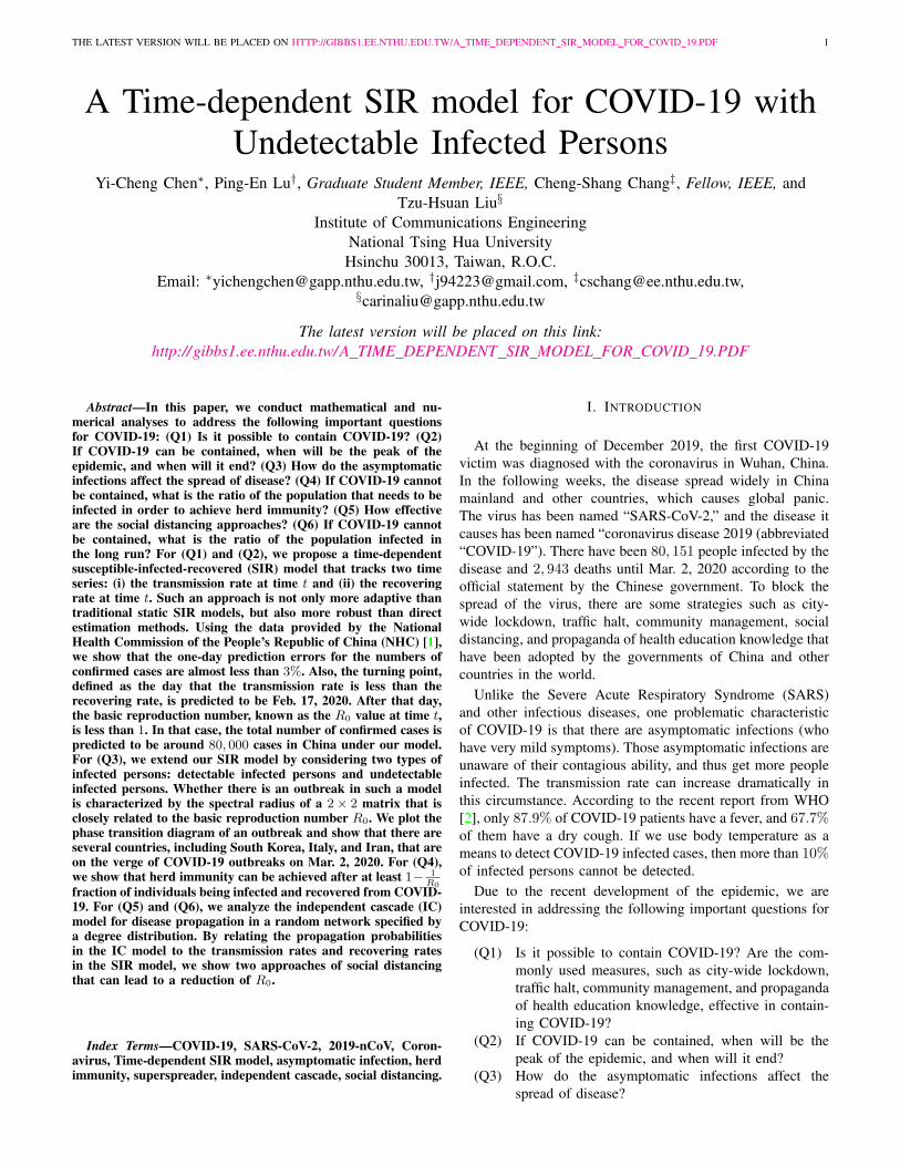
In Figure 2, we show the time evolution of the numberof infected persons and the number of recovered persons.The circle-marked solid curves are the real historical databy Mar. 2, 2020, and the star-marked dashed curves are ourprediction results for the future. The prediction results implythat the disease will end in 6 weeks, and the number of thetotal confirmed cases would be roughly 80, 000 if the Chinesegovernment remains their control policy, such as city-widelockdown and suspension of works and classes.

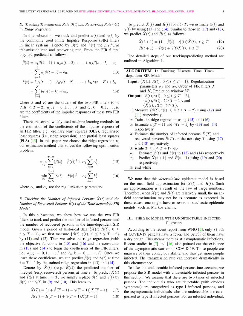
In Figure 3, we show the measured β(t) and γ(t) from thereal historical data. We can see that β(t) decreases dramati-cally, and γ(t) increases slightly. This is a direct result of theChinese government that tries to suppress the transmission rateβ(t) by city-wide lockdown and traffic halt. On the other hand,due to the lack of effective drugs and vaccines for COVID-19,the recovering rate γ(t) grows relatively slowly. Additionally,there is a definition change of the confirmed case on Feb. 12,2020 that makes the data related to Feb. 11, 2020 have noreference value. We mark these data points for β(t) and γ(t)with the gray dashed curve.

In an epidemic model, one crucial question is whether thedisease can be contained and the epidemic will end, or whetherthere will be a pandemic that infects a certain fraction of thetotal population n. To answer this, one commonly used metricis the basic reproduction number R0 that is defined as theaverage number of additional infections by an infected personbefore it recovers. In the classical SIR model, R0 is simplyβ/γ as an infected person takes (on average) 1/γ days torecover, and during that period time, it will be in contact with



��

��

��

��

��

��

��

��

��

��

��

��

��

��

�

��

��

��

��

��

��

��

��

� ��

��X(t)

X(t)R(t)

R(t)

Figure 2: Time evolution of the time-dependent SIR modelof the COVID-19. The circle-marked solid curve with darkorange (resp. green) color is the real number of infectedpersons X(t) (resp. recovered persons R(t)), the star-markeddashed curve with light orange (resp. green) color is thepredicted number of infected persons X(t) (resp. recoveredR(t) persons).

��

��

��

��

��

��

��

��

��

��

��

��

��

��

��

��

��

��

��

��

��

��

��

��

��

�� β�� γ

Figure 3: Measured transmission rate β(t) and recoveringrate γ(t) of the COVID-19 from Jan. 15, 2020 to Feb. 19,2020. The two curves are measured according to (12) and(11) respectively.

(on average) β persons. In our time-dependent SIR model,the basic reproduction number R0(t) is a function of time,and it is defined as β(t)/γ(t). If R0(t) > 1, the disease willspread exponentially and infects a certain fraction of the totalpopulation n. On the contrary, the disease will eventually becontained. Therefore, by observing the change of R0(t) withrespect to time or even predicting R0(t) in the future, we cancheck whether certain epidemic control policies are effectiveor not.

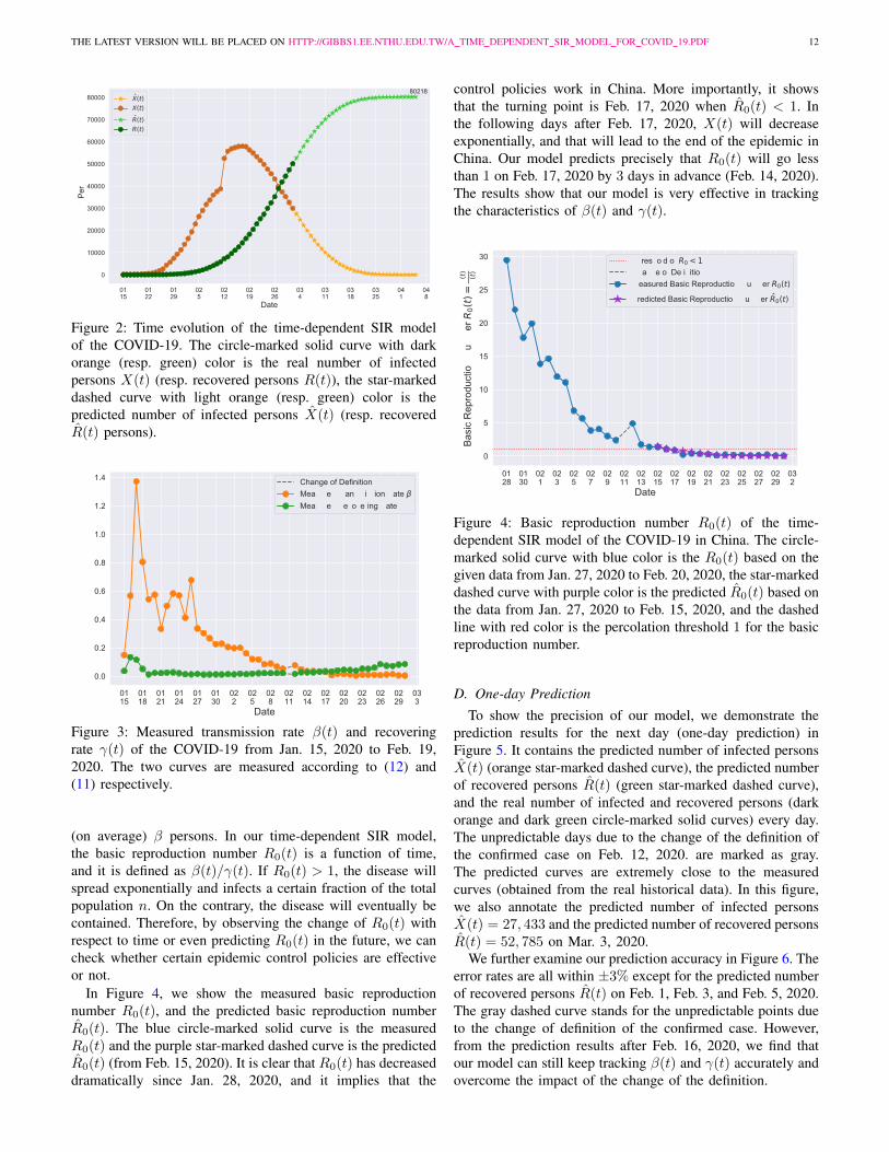
In Figure 4, we show the measured basic reproductionnumber R0(t), and the predicted basic reproduction numberR0(t). The blue circle-marked solid curve is the measuredR0(t) and the purple star-marked dashed curve is the predictedR0(t) (from Feb. 15, 2020). It is clear that R0(t) has decreaseddramatically since Jan. 28, 2020, and it implies that the

control policies work in China. More importantly, it showsthat the turning point is Feb. 17, 2020 when R0(t) < 1. Inthe following days after Feb. 17, 2020, X(t) will decreaseexponentially, and that will lead to the end of the epidemic inChina. Our model predicts precisely that R0(t) will go lessthan 1 on Feb. 17, 2020 by 3 days in advance (Feb. 14, 2020).The results show that our model is very effective in trackingthe characteristics of β(t) and γ(t).

��

��

��

��

��

��

��

��

��

��

��

��

��

��

��

��

��

��

��!�

�

�

��

��

��

��

��

� ��

��"

�!�� "�

��R

0(t)=

β(t)

γ(t)

�� R0<1��!�� "�� "�!�� "��R0(t)��!�� "�!�� "�� R0(t)

Figure 4: Basic reproduction number R0(t) of the time-dependent SIR model of the COVID-19 in China. The circle-marked solid curve with blue color is the R0(t) based on thegiven data from Jan. 27, 2020 to Feb. 20, 2020, the star-markeddashed curve with purple color is the predicted R0(t) based onthe data from Jan. 27, 2020 to Feb. 15, 2020, and the dashedline with red color is the percolation threshold 1 for the basicreproduction number.

D. One-day PredictionTo show the precision of our model, we demonstrate the

prediction results for the next day (one-day prediction) inFigure 5. It contains the predicted number of infected personsX(t) (orange star-marked dashed curve), the predicted numberof recovered persons R(t) (green star-marked dashed curve),and the real number of infected and recovered persons (darkorange and dark green circle-marked solid curves) every day.The unpredictable days due to the change of the definition ofthe confirmed case on Feb. 12, 2020. are marked as gray.The predicted curves are extremely close to the measuredcurves (obtained from the real historical data). In this figure,we also annotate the predicted number of infected personsX(t) = 27, 433 and the predicted number of recovered personsR(t) = 52, 785 on Mar. 3, 2020.

We further examine our prediction accuracy in Figure 6. Theerror rates are all within ±3% except for the predicted numberof recovered persons R(t) on Feb. 1, Feb. 3, and Feb. 5, 2020.The gray dashed curve stands for the unpredictable points dueto the change of definition of the confirmed case. However,from the prediction results after Feb. 16, 2020, we find thatour model can still keep tracking β(t) and γ(t) accurately andovercome the impact of the change of the definition.



��

��

��

��

��

��

��

��

��

��

��

��

��

��

��

��

��

��

�

��

��

��

��

��

��

��

��

��

��X(t)X(t)

R(t)R(t)

��

Figure 5: One-day prediction for the number of infected andrecovered persons. The unpredictable points due to the changeof definition of the confirmed case are marked as gray. Thecircle-marked solid curve with dark orange (resp. green) coloris the real number of infected persons X(t) (resp. recoveredpersons R(t)), the star-marked dashed curve with light orange(resp. green) color is the predicted number of infected personsX(t) (resp. recovered persons R(t)).

��

��

��

��

��

��

��

��

��

��

��

��

��

��

��

��

��

��%��%��%��%��%�%��%�%�%%�%��%��%��%��%

��

��

��%�

�� !��

Figure 6: Errors of the one-day prediction of the number ofinfected and recovered persons. The unpredictable points dueto the change of definition of the confirmed case on Feb. 12,2020 are marked as the gray dash curve.

E. Connections to the Wuhan City Lockdown

In this subsection, we show the connections between theepidemic prevention policies issued by the Chinese govern-ment and the historical data of the time-varying transmissionrates.

As shown in Figure 3, the disease has been graduallycontrolled in China as time goes on. Excluding the smallnumber of cases (X(t) < 500) before Jan. 21, 2020 (thatcauses the curve to fluctuate a lot), it is notable that β(t)increases gradually then drops dramatically during Jan. 23,2020 to Jan. 28, 2020, and it reaches the peak point on Jan.26, 2020, which coincides with the trends of the moving out inWuhan during the Chunyun (Spring Festival travel season) [20]

in Figure 7. Especially, the emigration trend is almost the sameas the β(t) during Jan. 20, 2020 to Jan. 25, 2020. We speculatethat people rushed into the public transportation system whenthe announcement of the Wuhan city lockdown was out, whichsignificantly increases the contact among people and speeds upthe spread of the virus. As a result of that, the transmissionrate β(t) increases substantially. As pointed out in Zhong’sstudy [21], the median of the incubation period of COVID-19is 3 days among 1099 valid confirmed cases, which makes theemigration trend aligns with β(t) if the extra 3 days are takeninto account. Finally, the disease is gradually getting undercontrol after the lockdown. The basic reproduction numberR0(t) is less than 1, i.e., β(t) < γ(t) since Feb. 17, 2020.

Figure 7: Trends of moving out during the Chunyun (SpringFestival travel season) in Wuhan city. The vertical axisrepresents the ratio between the number of people leavingthe city and the resident population in Wuhan. The orangecurve shows the ratio in 2019, while the blue curve showsthe ratio in 2020. We redraw this figure by our-self fromhttps://qianxi.baidu.com/ [20].

F. Basic Reproduction Numbers of Several Other Countries

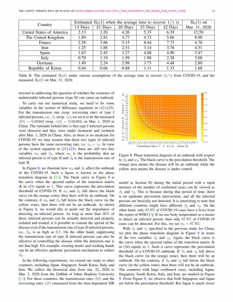
In addition to the dataset for China, we also measure thebasic reproduction number R0(t) on Mar. 31, 2020 for severalcountries from the datasets in [12]. This is shown in the lastcolumn of Table II. As the data for the cumulative numbers ofrecovered persons for these countries are noisy, we also showthe estimated R0(t) under various assumptions of the averagetime to recover 1/γ. The R0(t) values for the five countries,including United States of America, the United Kingdom,France, Iran, and Spain are very high. On the other hand, itseems that Italy is gaining control of the spread of the diseaseafter the Italian government announces the lockdown andforbids the gatherings of people on Mar. 10, 2020. Also, bothGermany and Republic of Korea are capable of controlling thespread of the disease.

G. The Effects of Type II Infected Persons

In this subsection, we show how undetectable (type II)infected persons affect the epidemic. In particular, we are in-


https://qianxi.baidu.com/


Country Estimated R0(t) when the average time to recover 1/γ is R0(t) onMar. 31, 202014 Days 21 Days 28 Days 35 Days 42 Days

United States of America 2.13 3.20 4.26 5.33 6.39 12.59The United Kingdom 1.89 2.83 3.77 4.72 5.66 8.90

France 2.58 3.86 5.15 6.44 7.73 4.76Iran 1.25 1.88 2.51 3.14 3.76 4.51

Spain 1.63 2.45 3.27 4.08 4.90 3.47Italy 0.79 1.19 1.59 1.98 2.38 3.08

Germany 1.49 2.24 2.98 3.73 4.48 2.80Republic of Korea 0.44 0.66 0.88 1.11 1.33 1.68

Table II: The estimated R0(t) under various assumptions of the average time to recover (1/γ) from COVID-19, and themeasured R0(t) on Mar. 31, 2020.

terested in addressing the question of whether the existence ofundetectable infected persons (type II) can cause an outbreak.

To carry out our numerical study, we need to fix somevariables in the system of difference equations in (21)-(23).For the transmission rate (resp. recovering rate) of type Iinfected persons, i.e., β1 (resp. γ1), we set it to be the measuredβ(t) = 0.00383 (resp. γ(t) = 0.08493) on Mar. 1, 2020 inChina. The rationale behind this is that type I infected personswere detected and they were under treatment and isolationafter Mar. 1, 2020 in China. Also, as there is no medicine forCOVID-19, we may assume that these two types of infectedpersons have the same recovering rate, i.e, γ2 = γ1. In viewof the system equation in (21)-(23), there are still two freevariables w2 and β2, where w2 is the probability that aninfected person is of type II and β2 is the transmission rate oftype II.

In Figure 8, we illustrate how w2 and β2 affect the outbreakof the COVID-19. Such a figure is known as the phasetransition diagram in [11]. The black curve in Figure 8 isthe curve when the spectral radius of the transition matrixA in (24) equals to 1. This curve represents the percolationthreshold of COVID-19. If w2 and β2 fall above the blackcurve (in the orange zone), then there will be an outbreak. Onthe contrary, if w2 and β2 fall below the black curve (in theyellow zone), then there will not be an outbreak. As shownin Figure 8, we would like to point out the importance ofdetecting an infected person. As long as more than 90% ofthose infected persons can be actually detected and properlyisolated and treated, it is possible to contain the spread of thedisease even if the transmission rate of type II infected persons,i.e., β2, is as high as 0.7. On the other hand, suppressingthe transmission rate of type II infected persons can also beeffective in controlling the disease while the detection rate isnot that high. For example, wearing masks and washing handscan be an effective epidemic prevention mechanism to reduceβ2.

In the following experiments, we extend our study to othercountries, including Japan, Singapore, South Korea, Italy, andIran. We collect the historical data from Jan. 22, 2020 toMar. 2, 2020 from the GitHub of Johns Hopkins University[12]. For these countries, the transmission rates β(t) and therecovering rates γ(t) (measured from the time-dependent SIR

��

��

��

��

��

��

��

��

��

��

��

��

��

��

��

��

��

��

��

��

��

�� !�� β2�

��

��

��

��

��

��

��

��

��

��

��

��

!� �

� ��

��

� ��

��

��

��

!��

��w

2�

��

��

��

��

��

��

��

��

��

Figure 8: Phase transition diagram of an outbreak with respectto β2 and w2. The black curve is the percolation threshold. Theorange area means the disease will be an outbreak while theyellow area means the disease is under control.

model in Section II) during the initial period with a rapidincrease of the number of confirmed cases can be viewed asβ2 and γ2. This is because during that period of time, thereis no epidemic prevention intervention, and all the infectedpersons are basically not detected. It is interesting to note thatdifferent countries might have different β2 and γ2. On theother hand, only 87.9% of COVID-19 cases have a fever fromthe report of WHO [2]. If we use body temperature as a meansto detect an infected person, then only 87.9% of COVID-19cases can be detected. For this, we set w1 = 87.9%.

With β1 and γ1 specified in the previous study for China,we plot the phase transition diagram in Figure 9 in termsof the two variables β2 and γ2. Again, the black curve isthe curve when the spectral radius of the transition matrix Ain (24) equals to 1. Such a curve represents the percolationthreshold of a COVID-19 outbreak. If β2 and γ2 fall abovethe black curve (in the orange zone), then there will be anoutbreak. On the contrary, if β2 and γ2 fall below the blackcurve (in the yellow zone), then there will not be an outbreak.The countries with large confirmed cases, including Japan,Singapore, South Korea, Italy, and Iran, are marked in Figure9. From Figure 9, we observe that both Singapore and Japanare below the percolation threshold. But Japan is much closer



to the percolation threshold. On the other hand, both SouthKorea and Italy are above the percolation threshold, and theyare on the verge of a potential outbreak on Mar. 2, 2020.These two countries must implement epidemic preventionpolicies urgently. Not surprisingly, on Mar. 10, 2020, theItalian government announces the lockdown and forbids thegatherings of people. It is worth mentioning that there are twomarks for Iran in the Figure. The one above the percolationthreshold is the one without adding the number of deaths intothe number of recovered persons. The other one below thepercolation threshold is the one that adds the number of deathsinto the number of recovered persons. For some unknownreason, the death rate in Iran is higher than the other countries.The high death rate seems to prevent an outbreak in Iran.

��

��

��

��

��

��

��

��

��

��

��

��

��

��

��

��

��

��

��

��

��

�#� $��$$�! �#�%��!��)"�� %��"�#$! $��β2�

��

��!'�#� ��#�%��!��

)"�� %��

�"�#$! $��γ

2�

�!&%��!#��

��"�

�� "!#�

�%��)

�#� �(��%�$�

�#� �(�!��%�$�

��

��

��

��

��

��

��

��

��

Figure 9: Phase transition diagram of an outbreak with respectto β2 and γ2. The black curve is the percolation threshold. Theorange area means the disease will be an outbreak, while theyellow area means the disease is under control.

H. The Effects of Social Distancing

In this subsection, we show the numerical results of thesocial distancing approach that cancels mass gatherings byremoving nodes with the number of edges larger than orequal to k0. As shown in Theorem 5, the basic reproduction

number is reduced by a factor of∑k0−2k=0 kqk∑∞k=0 kqk

, where qk is

the excess degree distribution of pk. For this experiment, weuse the dataset collected by [22] from Facebook. This datasetrepresents the verified Facebook page (with blue checkmark)networks of the artist category. The blue checkmark meansFacebook has confirmed that an account is the authenticpresence of the public figure, celebrity, or global brand itrepresents. Each node in the network represents the page,and edges between two nodes are mutual likes among them.This dataset is composed of 50, 515 nodes and 819, 306 edges.Some other properties are listed as follow: mean degree 32.4,max degree 1, 469, diameter 11, and clustering coefficient0.053. In Figure 10, we show the log-log plots of the degreedistribution and the excess degree distribution of this dataset.The degree distribution appears to be a (truncated) Paretodistribution with the exponent 1.69 (the slope in the figure).

��

��

��

��

��

��

��

��

��

� ��

��

��

��

�� Pk�� qk

Figure 10: The degree distribution and the excess degreedistribution of the Facebook dataset.

In Figure 11, we plot the reduction ratio∑k0−2


asa function of k0. The ratio is between 0 and 1, and it ismonotonically increasing in k0. Using the R0 values (on Mar.31, 2020) in the last column of Table II, we also show thatthe minimum k0s to prevent an outbreak in Italy, U.S., andSouth Korea are 63, 195, and 435, respectively; moreover, theaffected fraction of tail distributions are 13.1%, 2.2%, and0.4%, respectively. In particular, if canceling mass gatheringis the only measure used for controlling COVID-19 in the U.S.with the R0 value of 12.59 on Mar. 31, 2020, then one canprevent an outbreak by “removing” all the nodes with degreeslarger than or equal to 63 (in the Facebook dataset), and theremoval might affect 13.1% of the nodes in the Facebookdataset.

� �� k0

��

��

��

��

��

��

��

��

��

� ��

�� "��! ��

Figure 11: The reduction ratio∑k0−2


as a function of k0.The minimum k0s to prevent an outbreak in Italy, U.S., andSouth Korea are 63, 195, and 435, respectively.

I. The Ratio of the Population Infected in the Long Run

In this subsection, we show the numerical results of theratio of the population infected in the long run in Subsection



IV-D. As shown in Theorem 6, if R0 > 1, then there is anonzero probability r that a randomly selected node is infectedin the long run. In Figure 12, we plot the infected probabilityr as a function of R0 for various degree distributions. For thisnumerical experiment, we use the same Facebook dataset inthe previous subsection. Note that the mean degree and themean excess degree of this Facebook dataset are 32.4 and155.6, respectively. We also generate three random networks:two from the Erdos-Renyi (ER) model [23] with the meandegrees c = 32 and c = 155, and one from the Barabasi-Albert (BA) model [24] with the mean degree c = 32. Thenumbers of nodes are all set to 50, 000. The degree distributionof the BA model (generated by using the linear preferentialattachment rule) is known to follow the asymptotic power-lawdistribution with pk ≈ k−3 for large k’s. The mean excessdegree of the BA model is 84.05.

From Figure 12, one can see that there is an outbreak whenR0 > 1. The probability r is increasing in R0. Also, as shownin this figure, the two curves of the two ER models (evenwith different mean degrees) overlap with each other. Thatmeans that r is independent of the mean degree when thedegree distribution is Poisson (as shown in (72) at the end ofSubsection IV-D).

On interesting observation is that the infected probability rof the ER model is larger than the infected probabilities ofthe other networks with the power-law degree distributions,i.e., the Facebook dataset and the BA model. This is becausewe relate the propagation probability φ by R0/g

′1(1) in (70)

(to ensure that the average number of additional infections byan infected person in the IC model is the same as that in theSIR model). Thus, a network with a large mean excess degreeg′1(1) has a low propagation probability φ (when R0 is fixed).That leads to a smaller ratio of the population infected in thelong run. To explain this further, we note that the probabilityof having a super spreader (a node with a very large degree) ina network with a power-law degree distribution is higher thanthat of the ER model. A super spreader is capable of infectinga large number of its first neighbors. However, the neighbors ofa super spreader tend to have relatively low degrees (contacts)than that of a super spreader. As such, it makes the diseasemore difficult to spread further in the IC model. On the otherhand, the probability of having a super spreader in the ERmodel is exponentially small. Since the infected subgraphappears to be a tree (if one follows an edge of an infectednode to propagate the disease to the other nodes in the ICmodel), the disease may spread slowly in the early stage ofthe epidemic in the ER model than that in the BA model.However, if R0 > 1, the disease may continue to propagatein the ER model to a larger fraction of the total population inthe long run. For example, when R0 = 3, the percentage ofinfected persons is more than 90% in the ER model.

VI. DISCUSSIONS AND SUGGESTIONS

As of Mar. 2, 2020, it seems that COVID-19 has beengradually controlled in China since the prevention policies,such as city-wide lockdown was issued in China in Jan. 2020.Although the policies such as traffic halt, small community

0.5 1.0 1.5 2.0 2.5 3.0R0

0.0

0.2

0.4

0.6

0.8

r

ER model with c= 155ER model with c= 32BA modelFacebook dataset

Figure 12: The probability r that a randomly selected node isinfected in the long run as a function of R0 for various degreedistributions.

management, and city-wide lockdown can effectively reducethe transmission rates β1 and β2; however, these relativelyextreme policies not only restrict the right of personal freedombut also affect the normal operation of society. These extremepolicies forced several companies and factories to halt produc-tion, which impacts all sectors of the economy. Therefore, tostrike a balance between the prevention of disease and ensuringthe normal operation of society is crucial, and it is importantto suggest the so-called “optimal” control policies.

For this, we would like to put forward some discussions andsuggestions for controlling the spread of COVID-19 based onthe observation made from the results of our system models.From our results in Theorem 1, Corollary 2, Theorem 3,Corollary 4, and Theorem 5, we know that there is no outbreakfor a disease if

h · s · (w1β1γ1

+ w2β2γ2

) < 1, (73)

where h is the herd immunity reduction factor in Corollary 2when 1−h fraction of individuals are immune to the disease,s is the social distancing reduction factor in Corollary 4 orTheorem 5, w1 (resp. w2) is the probability that an infectedperson can (resp. cannot) be detected, and β1 and γ1 (resp.β2 and γ2) are the transmission rate and the recovering rateof an infected person who can (resp. cannot) be detected. ForCOVID-19, β1 ≤ β2 and γ1 ≥ γ2 as an infected person, oncedetected, can be treated (to shorten the recovery time) andisolated (to reduce the transmission rate). As w1 +w2 = 1, itis thus preferable to have a much larger w1 than w2.

To prevent an outbreak, one should minimize the value onthe left-hand side of (73). Here we discuss several approachesfor that.

1. Increasing the recovering rate γ1: the most effective wayto increase γ1 is to find anti-virus drugs; however, it takestime. Hence, we should focus on the other approaches tocontrol the spread of the disease in this stage.

2. Reducing the herd immunity reduction factor h: the mosteffective way for this is to find vaccines to reduce thefraction of susceptible persons. Once again, it takes time,



and we should focus on the other approaches to controlthe spread of the disease in this stage.

3. Decreasing the transmission rate β1: once an infectedperson is detected, it should be isolated to avoid extrainfection on society and lower the transmission rateβ1. Quarantine of the persons who are suspected to bein contact with infected persons could also lower thetransmission rates β1 and β2.

4. Increasing the detection probability w1 (and thus reducingw2): mass testing can certainly increase w1. In fact,South Korea did an outstanding job of drive-thru testing.If mass testing is not possible due to the limitation ofmedical resources, then measuring body temperature canalso be an effective alternative, as 87.9% of the confirmedcases of COVID-19 have a fever. In addition to this,one can also track the travel history, occupation, contact,and cluster (TOCC) of the confirmed cases to narrowthe range of the possible sources. These sources mightcontain asymptomatic infected persons, and testing theclose contacts of these possible sources can thus increasew1 by detecting asymptomatic infected persons.

5. Decreasing the transmission rate β2: propaganda of healtheducation knowledge can reduce the transmission rate β2substantially. For example, wearing masks in public andenclosed space, washing hands, avoiding touching yourmouth, eyes, and nose are good ways to not only pro-tect ourselves from being infected by the asymptomaticinfected persons but also avoid infecting others.

6. Reducing the social distancing reduction factor s: asshown in Corollary 4 and Theorem 5, there are twopractical approaches that can reduce the social distancingreduction factor s: (i) allowing every person to keepits interpersonal contacts up to a fraction of its normalcontacts, and (ii) canceling mass gatherings.

VII. CONCLUSION AND FUTURE WORK

In this paper, we conducted mathematical and numericalanalyses for COVID-19. Our time-dependent SIR model is notonly more adaptive than traditional static SIR models, but alsomore robust than direct estimation methods. Our numericalresults show that one-day prediction errors for the number ofinfected persons X(t) and the number of recovered personsR(t) are within (almost) 3% for the dataset collected fromthe National Health Commission of the People’s Republic ofChina (NHC) [1]. Moreover, we are capable of tracking thecharacteristics of the transmission rate β(t) and the recoveringrate γ(t) with respect to time t, and precisely predict the futuretrend of the COVID-19 outbreak in China.

To address the impact of asymptomatic infections inCOVID-19, we extended our SIR model by considering twotypes of infected persons: detectable infected persons andundetectable infected persons. Whether there is an outbreakin such a model is characterized by the spectral radius of a2 × 2 matrix that is closely related to the basic reproductionnumber R0. In addition to our numerical analysis for China,we further extended our study to other countries, includingJapan, Singapore, South Korea, Italy, and Iran.

To understand the effects of social distancing approaches,including the reduction of interpersonal contacts and cancelingmass gatherings, we analyzed the IC model for disease propa-gation in the configuration model. By relating the propagationprobabilities in the IC model to the transmission rates andrecovering rates in the SIR model, we showed these socialdistancing approaches can lead to a reduction of R0.

Last but not least, based on the experimental results, somediscussions and suggestions on epidemic prevention are pro-posed from the perspective of our models. In the future, wewould like to extend our deterministic SIR model by usingstochastic models, such as the non-homogeneous Markovchain, to further improve the precision of the prediction results.

REFERENCES

[1] “Outbreak notification,” Jan 2020. [Online]. Available: http://www.nhc.gov.cn/xcs/yqtb/list gzbd.shtml

[2] “Coronavirus disease (covid-19) outbreak,” Jan 2020. [Online]. Avail-able: https://www.who.int/emergencies/diseases/novel-coronavirus-2019

[3] I. Nesteruk, “Statistics based predictions of coronavirus 2019-ncovspreading in mainland china,” MedRxiv, 2020.

[4] Y. Chen, J. Cheng, Y. Jiang, and K. Liu, “A time delay dynamicalmodel for outbreak of 2019-ncov and the parameter identification,” arXivpreprint arXiv:2002.00418, 2020.

[5] L. Peng, W. Yang, D. Zhang, C. Zhuge, and L. Hong, “Epidemicanalysis of covid-19 in china by dynamical modeling,” arXiv preprintarXiv:2002.06563, 2020.

[6] T. Zhou, Q. Liu, Z. Yang, J. Liao, K. Yang, W. Bai, X. Lu, and W. Zhang,“Preliminary prediction of the basic reproduction number of the wuhannovel coronavirus 2019-ncov,” Journal of Evidence-Based Medicine,2020.

[7] B. F. Maier and D. Brockmann, “Effective containment explains sub-exponential growth in confirmed cases of recent covid-19 outbreak inmainland china,” arXiv preprint arXiv:2002.07572, 2020.

[8] S. Zhao, Q. Lin, J. Ran, S. S. Musa, G. Yang, W. Wang, Y. Lou, D. Gao,L. Yang, D. He et al., “Preliminary estimation of the basic reproductionnumber of novel coronavirus (2019-ncov) in china, from 2019 to 2020:A data-driven analysis in the early phase of the outbreak,” InternationalJournal of Infectious Diseases, 2020.

[9] T. Zeng, Y. Zhang, Z. Li, X. Liu, and B. Qiu, “Predictions of 2019-ncov transmission ending via comprehensive methods,” arXiv preprintarXiv:2002.04945, 2020.

[10] Z. Hu, Q. Ge, L. Jin, and M. Xiong, “Artificial intelligence forecastingof covid-19 in china,” arXiv preprint arXiv:2002.07112, 2020.

[11] M. Newman, Networks: An Introduction. Oxford University Press,2010.

[12] CSSEGISandData and J. H. University, “Covid-19,” Feb 2020. [Online].Available: https://github.com/CSSEGISandData/COVID-19

[13] D. Kempe, J. Kleinberg, and E. Tardos, “Maximizing the spread ofinfluence through a social network,” in Proceedings of the ninth ACMSIGKDD international conference on Knowledge discovery and datamining. ACM, 2003, pp. 137–146.

[14] A. Y. Ng, A. X. Zheng, and M. I. Jordan, “Stable algorithms for linkanalysis,” in Proceedings of the 24th annual international ACM SIGIRconference on Research and development in information retrieval, 2001,pp. 258–266.

[15] B. S. Dayal and J. F. MacGregor, “Identification of finite impulseresponse models: methods and robustness issues,” Industrial & engi-neering chemistry research, vol. 35, no. 11, pp. 4078–4090, 1996.

[16] T. Ganyani, C. Kremer, D. Chen, A. Torneri, C. Faes, J. Wallinga,and N. Hens, “Estimating the generation interval for covid-19 basedon symptom onset data,” medRxiv, 2020.

[17] C.-J. Chen, Epidemiology: Principles and Methods. Linking PublishingCompany, 1999.

[18] N. G. Becker, Modeling to inform infectious disease control. CRCPress, 2015, vol. 74.

[19] F. Pedregosa, G. Varoquaux, A. Gramfort, V. Michel, B. Thirion,O. Grisel, M. Blondel, P. Prettenhofer, R. Weiss, V. Dubourg, J. Vander-plas, A. Passos, D. Cournapeau, M. Brucher, M. Perrot, and E. Duch-esnay, “Scikit-learn: Machine learning in Python,” Journal of MachineLearning Research, vol. 12, pp. 2825–2830, 2011.


http://www.nhc.gov.cn/xcs/yqtb/list_gzbd.shtml

http://www.nhc.gov.cn/xcs/yqtb/list_gzbd.shtml

https://www.who.int/emergencies/diseases/novel-coronavirus-2019

https://github.com/CSSEGISandData/COVID-19


[20] “Real-time big data report of covid-19 outbreak.” [Online]. Available:https://voice.baidu.com/act/newpneumonia/newpneumonia

[21] W.-J. Guan, Z.-Y. Ni, Y. Hu, W.-H. Liang, C.-Q. Ou, J.-X. He, L. Liu,H. Shan, C.-L. Lei, D. S. Hui et al., “Clinical characteristics of 2019novel coronavirus infection in china,” medRxiv, 2020.

[22] B. Rozemberczki, R. Davies, R. Sarkar, and C. Sutton, “Gemsec:Graph embedding with self clustering,” in Proceedings of the 2019IEEE/ACM International Conference on Advances in Social NetworksAnalysis and Mining 2019. ACM, 2019, pp. 65–72. [Online]. Available:https://snap.stanford.edu/data/gemsec-Facebook.html

[23] P. Erdos, “On random graphs,” Publicationes mathematicae, vol. 6, pp.290–297, 1959.

[24] A.-L. Barabasi and R. Albert, “Emergence of scaling in random net-works,” science, vol. 286, no. 5439, pp. 509–512, 1999.

Yi-Cheng Chen received his B.S. degree in electri-cal engineering from National Taiwan University ofScience and Technology, Taipei, Taiwan (R.O.C.), in2018. He is currently pursuing the M.S. degree in theInstitute of Communications engineering, NationalTsing-Hua University, Hsinchu, Taiwan (R.O.C.).

Ping-En Lu (GS’17) received his B.S. degree incommunication engineering from the Yuan Ze Uni-versity, Taoyuan, Taiwan (R.O.C.), in 2015. He iscurrently pursuing the Ph.D. degree in the Insti-tute of Communications Engineering, National TsingHua University, Hsinchu, Taiwan (R.O.C.). He wonthe ACM Multimedia 2017 Social Media Prediction(SMP) Challenge with his team in 2017. His researchinterest is in network science, efficient clusteringalgorithms, network embedding, and deep learningalgorithms. He is an IEEE Graduate Student Mem-

ber.

Cheng-Shang Chang (S’85-M’86-M’89-SM’93-F’04) received the B.S. degree from National TaiwanUniversity, Taipei, Taiwan, in 1983, and the M.S.and Ph.D. degrees from Columbia University, NewYork, NY, USA, in 1986 and 1989, respectively, allin electrical engineering.

From 1989 to 1993, he was employed as aResearch Staff Member with the IBM Thomas J.Watson Research Center, Yorktown Heights, NY,USA. Since 1993, he has been with the Departmentof Electrical Engineering, National Tsing Hua Uni-

versity, Taiwan, where he is a Tsing Hua Distinguished Chair Professor. He isthe author of the book Performance Guarantees in Communication Networks(Springer, 2000) and the coauthor of the book Principles, Architectures andMathematical Theory of High Performance Packet Switches (Ministry ofEducation, R.O.C., 2006). His current research interests are concerned withnetwork science, big data analytics, mathematical modeling of the Internet,and high-speed switching.

Dr. Chang served as an Editor for Operations Research from 1992 to1999, an Editor for the IEEE/ACM TRANSACTIONS ON NETWORKING from2007 to 2009, and an Editor for the IEEE TRANSACTIONS ON NETWORKSCIENCE AND ENGINEERING from 2014 to 2017. He is currently serving asan Editor-at-Large for the IEEE/ACM TRANSACTIONS ON NETWORKING.He is a member of IFIP Working Group 7.3. He received an IBM OutstandingInnovation Award in 1992, an IBM Faculty Partnership Award in 2001, andOutstanding Research Awards from the National Science Council, Taiwan, in1998, 2000, and 2002, respectively. He also received Outstanding TeachingAwards from both the College of EECS and the university itself in 2003. Hewas appointed as the first Y. Z. Hsu Scientific Chair Professor in 2002. Hereceived the Merit NSC Research Fellow Award from the National ScienceCouncil, R.O.C. in 2011. He also received the Academic Award in 2011and the National Chair Professorship in 2017 from the Ministry of Education,R.O.C. He is the recipient of the 2017 IEEE INFOCOM Achievement Award.

Tzu-Hsuan Liu received the B.S. degree in com-munication engineering from National Central Uni-versity, Taoyuan, Taiwan (R.O.C.), in 2018. She iscurrently pursuing the M.S. degree in the Institute ofCommunications Engineering, National Tsing HuaUniversity, Hsinchu, Taiwan (R.O.C.). Her researchinterest is in 5G wireless communication.


https://voice.baidu.com/act/newpneumonia/newpneumonia

https://snap.stanford.edu/data/gemsec-Facebook.html

Documents

A Time-dependent SIR model for COVID-19 with Undetectable