Embed Size (px)
Citation preview
1
A Total Cost of Ownership Model for Low Temperature PEM Fuel Cells in Combined Heat and Power and Backup Power Applications Nadir Saggiorato, Max Wei, Timothy Lipman1, Ahmad Mayyas1, Shuk Han Chan2, Hanna Breunig, Thomas McKone, Paul Beattie3, Patricia Chong3, Whitney G. Colella4, Brian D. James4
Environmental Energy Technologies Division Updated November 2016
1University of California, Berkeley, Transportation Sustainability Research Center, Berkeley, California 2University of California, Berkeley, Laboratory for Manufacturing and Sustainability, Department of Mechanical Engineering, Berkeley, California 3Ballard Power Systems 4Strategic Analysis, Inc. (SA), Energy Services Division, 4075 Wilson Blvd., Suite 200, Arlington VA 22203
This work was supported by the U.S. Department of Energy, Office of Energy Efficiency and Renewable Energy (EERE) Fuel Cells Technologies Office (FCTO) under Lawrence Berkeley National Laboratory Contract No. DE-AC02-05CH11231
ERNEST ORLANDO LAWRENCE
BERKELEY NATIONAL LABORATORY
2
DISCLAIMER
This document was prepared as an account of work sponsored by the United States Government. While this document is believed to contain correct information, neither the United States Government nor any agency thereof, nor The Regents of the University of California, nor any of their employees, makes any warranty, express or implied, or assumes any legal responsibility for the accuracy, completeness, or usefulness of any information, apparatus, product, or process disclosed, or represents that its use would not infringe privately owned rights. Reference herein to any specific commercial product, process, or service by its trade name, trademark, manufacturer, or otherwise, does not necessarily constitute or imply its endorsement, recommendation, or favoring by the United States Government or any agency thereof, or The Regents of the University of California. The views and opinions of authors expressed herein do not necessarily state or reflect those of the United States Government or any agency thereof, or The Regents of the University of California. Ernest Orlando Lawrence Berkeley National Laboratory is an equal opportunity employer.

3
ACKNOWLEDGEMENTS
The authors gratefully acknowledge the U.S. Department of Energy, Office of Energy Efficiency and Renewable Energy (EERE) Fuel Cells Technologies Office (FCTO) for their funding and support of this work. The authors would like to express their sincere thanks to Mickey Oros from Altergy Power Systems, Bob Sandbank from Eurotech, Mark Miller from Coating Tech Services, Geoff Melicharek and Nicole Fenton from ConQuip, Inc., and Charlene Chang from Richest Group (Shanghai, China) for their assistance and valuable inputs.
4
Executive Summary
A total cost of ownership model (TCO) is described for emerging applications in stationary fuel cell systems. Low temperature proton exchange membrane (LT PEM) systems for use in combined heat and power applications from 1 to 250 kilowatts-electric (kWe1) and backup power applications from 1 to 50 kWe are considered. The total cost of ownership framework expands the direct manufacturing cost modeling framework of other studies to include operational costs and life-cycle impact assessment of possible ancillary financial benefits during operation and at end-of-life. These include credits for reduced emissions of global warming gases such as carbon dioxide (CO2) and methane (CH4), reductions in environmental and health externalities, and end-of-life recycling. This report is an updated revision to the earlier 2014 LBNL report [1]. System designs and functional specifications for LT PEM fuel cell systems for back-up power and co-generation applications were developed across the range of system power levels above. Bottom-up cost estimates were made based on currently installed fuel cell systems for balance of plant (BOP) costs, and detailed evaluation of design-for-manufacturing-and-assembly2 (DFMA) costs was carried out to estimate the direct manufacturing costs for key fuel cell stack components. The costs of the fuel processor subsystem are also based on an earlier DFMA analysis [2]. The development of high throughput, automated processes achieving high yield are estimated to push the direct manufacturing cost per kWe for the fuel cell stack to nearly $200/kWe at high production volumes. Overall direct system costs including corporate markups and installation costs are about $2300/kWe ($1900/kWe) for 10kW (1000kW) CHP systems at 50,000 systems per year, and about $1100/kWe for 10kWe backup power systems at 50,000 systems per year. The updated values for system costs are within 10% of the 2014 report, but this overall similar cost result is derived from lower estimated stack costs and higher balance of plant costs. At high production volume, material costs dominate the cost of fuel cell stack manufacturing. Based on these stack costs, we find that BOP costs (including the fuel processor) dominate overall system direct costs for CHP systems and are thus a key area for further cost reduction. For CHP systems at low power, the fuel processing subsystem is the largest cost contributor of total non-stack costs. At high power, the electrical power subsystem is the dominant cost contributor. Life-cycle or use-phase modeling and life cycle impact assessment (LCIA) were carried out for regions in the U.S. with high-carbon intensity electricity from the grid. In other regions, TCO costs of fuel cell CHP systems relative to grid power exceed prevailing commercial power rates at the system sizes and production volumes studied here. Including total cost of ownership credits can give a net positive cash flow in Minneapolis and Chicago for fuel cell CHP systems in small hotels. We find this to be true for a static grid with unchanging grid emission factors, and also for a cleaner grid out to 2030 subject to federal regulations such as the EPA’s Clean Power Plan. TCO costs for fuel cell CHP systems are dependent on several factors such as the cost of natural gas, utility tariff structure, amount of waste heat utilization, carbon intensity of displaced electricity and conventional heating, carbon price, and valuation of health and environmental externalities. Quantification of externality damages to the environment and public health utilized earlier environmental impact assessment work and datasets available at LBNL. Overall, this type of total cost of ownership analysis quantification is important to identify key opportunities for direct cost reduction, to fully value the costs and benefits of fuel cell systems in stationary applications, and to provide a more comprehensive context for future potential policies.
1 In this report, units of kWe stand for net kW electrical power unless otherwise noted. 2 DFMA is a registered trademark of Boothroyd, Dewhurst, Inc. and is the combination of the design of manufacturing processes and design of assembly processes for ease of manufacturing and assembly and cost reduction.
5
Table of Contents
1 Introduction ..................................................................................................................... 12 1.1 Stationary fuel cell systems .................................................................................................. 12 1.2 Technical Targets and Technical Barriers ............................................................................... 13 1.3 Emerging applications .......................................................................................................... 13 1.4 Total Cost of Ownership Modeling ........................................................................................ 14
1.4.1 Other FC applications................................................................................................................. 15
2 System Design and Functional Specifications ..................................................................... 16 2.1 CHP System Design............................................................................................................... 16 2.2 CHP Functional Specifications ............................................................................................... 16 2.3 System and component lifetimes .......................................................................................... 18
3 Costing Approach and Considerations ............................................................................... 20 3.1 DFMA Costing Model Approach ............................................................................................ 20 3.2 Parameters for Manufacturing Cost Analysis ......................................................................... 24 3.3 Building considerations ........................................................................................................ 26 3.4 Yield considerations ............................................................................................................. 26 3.5 Scrap considerations ............................................................................................................ 26
4 DFMA Manufacturing Cost Analysis for CHP applications................................................... 27 4.1 Catalyst Coated Membrane (CCM) ........................................................................................ 27
4.1.1 CCM manufacturing process cost analysis ................................................................................ 29 4.1.2 CCM Manufacturing line process parameters ........................................................................... 33 4.1.3 CCM cost summary .................................................................................................................... 45 4.1.4 CCM manufacturing costs compared to LBNL cost results ........................................................ 47 4.1.5 CCM cost sensitivity ................................................................................................................... 48
4.2 Gas Diffusion Layer (GDL) ..................................................................................................... 51 4.2.1 GDL cost summary ..................................................................................................................... 52
4.3 MEA Frame/Seal .................................................................................................................. 53 4.3.1 MEA Frame/Seal cost summary ................................................................................................. 54
4.4 Carbon bipolar plates ........................................................................................................... 56 4.4.1 Carbon plates cost summary ..................................................................................................... 57
4.5 Stack assembly..................................................................................................................... 59 4.5.1 Stack assembly cost summary ................................................................................................... 60
4.6 CHP PEMFC stack manufacturing cost results ........................................................................ 61 4.7 Cost results comparison ....................................................................................................... 65
4.7.1 SA cost study .............................................................................................................................. 66 4.7.2 LBNL 2014 cost study ................................................................................................................. 66
4.8 Sensitivity analysis ............................................................................................................... 67
5 Balance Of Plant and System Costs .................................................................................... 73 5.1 Balance of plant results ........................................................................................................ 73 5.2 Fuel Cell System Direct Manufacturing Costs and Installed Cost Results ................................. 77 5.3 CHP Target Costs .................................................................................................................. 79
6 DFMA Manufacturing Cost Analysis for Backup Power Application .................................... 81 6.1 Introduction ......................................................................................................................... 81
6.1.1 Advantages of FC Backup Power ............................................................................................... 81 6.1.2 Fuel cell backup power system design ...................................................................................... 83
6.2 Catalyst Coated Membrane (CCM) ........................................................................................ 84 6.3 Metal bipolar plates ............................................................................................................. 86
6.3.1 Process flow description ............................................................................................................ 87
6
6.3.2 Metal plates Properties ............................................................................................................. 89 6.3.3 Metal plates cost summary ....................................................................................................... 92 6.3.4 Metal Bipolar Plate Cost Sensitivity ........................................................................................... 97 6.3.5 High speed Bipolar plates manufacturing................................................................................ 100 6.3.6 Pre-coated SS cost summary ................................................................................................... 103 6.3.7 High-Speed Considerations ...................................................................................................... 105 6.3.8 Pre-coated stainless steel manufactured in-house ................................................................. 106 6.3.9 Make vs. Buy Analysis for Metal Plates ................................................................................... 113
6.4 Stack assembly cost summary ............................................................................................ 115 6.5 GDL cost summary ............................................................................................................. 115 6.6 Frame-seal cost summary ................................................................................................... 116 6.7 Backup PEMFC stack manufacturing cost results ................................................................. 117 6.8 Backup PEMFC System Results ........................................................................................... 121 6.9 Cost Targets for Backup power system ............................................................................... 124
6.9.1 NREL 2014 Study ...................................................................................................................... 124 6.9.2 5kW backup cost model........................................................................................................... 127 6.9.3 Annual Production Volumes .................................................................................................... 128 6.9.4 Cost comparison with Reported Prices .................................................................................... 129
7 Life Cycle Impact Assessment .......................................................................................... 130 7.1 Regional Emissions Factors for CO2 and Criteria Pollutant Emission Rates ............................ 130 7.2 Updated Marginal Benefits of Abatement Valuation ........................................................... 132 7.3 Estimating a Cleaner Grid in 2030 ....................................................................................... 133 7.4 LCIA for the 2016-2030 Time Period .................................................................................... 134 7.5 LT PEM CHP in small hotels in Chicago and Minneapolis, 2016-2030 .................................... 135
8 Appendix ........................................................................................................................ 142 References ………………………………………………………………………………………………………………………………………..............125
7
List of Figures
Figure 1-1 Research and modeling approach. ........................................................................................................................................ 15 Figure 2-1 System design for CHP system using reformate fuel from LBNL ............................................................................ 16 Figure 3-1 Generalized roll-up steps for total system cost from LBNL ....................................................................................... 20 Figure 4-1 Platinum price trend over the last decade. ........................................................................................................................ 27 Figure 4-2 Nafion® membrane price ......................................................................................................................................................... 28 Figure 4-3 Nafion® Ionomer price from SA [3] ..................................................................................................................................... 29 Figure 4-4 CCM manufacturing process as in Wei et al. 2014. ........................................................................................................ 30 Figure 4-5 Slot die working principle ......................................................................................................................................................... 33 Figure 4-6 Patch coated membrane [12]................................................................................................................................................... 33 Figure 4-7 CCM percentage cost breakdown for 1kW system......................................................................................................... 46 Figure 4-8 CCM percentage cost breakdown for 100kW system ................................................................................................... 47 Figure 4-9 CCM manufacturing cost comparison .................................................................................................................................. 48 Figure 4-10 CCM sensitivity for 100kW and 100 systems/year ..................................................................................................... 49 Figure 4-11 CCM sensitivity for 100kW and 1000 systems/year .................................................................................................. 49 Figure 4-12 CCM sensitivity for 100kW and 10000 systems/year ............................................................................................... 50 Figure 4-13 CCM sensitivity for 100kW and 50000 systems/year ............................................................................................... 50 Figure 4-14 CCM sensitivity for 10kW and 100 systems/year ....................................................................................................... 51 Figure 4-15 GDL cost breakdown for 10kW system ............................................................................................................................ 52 Figure 4-16 GDL cost breakdown for 100kW system ......................................................................................................................... 52 Figure 4-17 Bordered or framed MEA from LBNL ................................................................................................................................ 54 Figure 4-18 MEA process flow from LBNL ............................................................................................................................................... 54 Figure 4-19 Percentage cost breakdown for MEA frame, for 10kW system ............................................................................. 55 Figure 4-20 Percentage cost breakdown for MEA frame, for 100kW system .......................................................................... 55 Figure 4-21 Carbon bipolar plate from LBNL ......................................................................................................................................... 56 Figure 4-22 Carbon bipolar plate process line. ...................................................................................................................................... 57 Figure 4-23 Percentage cost breakdown for carbon bipolar plate, for 10kW system .......................................................... 57 Figure 4-24 Percentage cost breakdown for carbon bipolar plate, for 100kW system ....................................................... 58 Figure 4-25 Carbon plate cost comparison ($/plate) .......................................................................................................................... 59 Figure 4-26 Assembly process line from LBNL ...................................................................................................................................... 59 Figure 4-27 Stack assembly cost vs. production volume expressed in ($/kW). ...................................................................... 61 Figure 4-28 Stack manufacturing cost variation with annual production rate in ($/kW).................................................. 62 Figure 4-29 Stack manufacturing cost variation with system size in ($/kW) .......................................................................... 62 Figure 4-30 PEMFC Stack cost as a function of annual production volume (systems/yr) for 10kW system ............. 63 Figure 4-31 PEMFC Stack cost as a function of annual production volume (systems/yr) for 100kW system .......... 63 Figure 4-32 Breakdown of the stack cost in a stack components level for 10kW system .................................................. 64 Figure 4-33 Breakdown of the stack cost in a stack components level for 100kW system ................................................ 64 Figure 4-34 Disaggregation of stack cost by relative percentage of components cost for 10 kW system ................... 65 Figure 4-35 Disaggregation of stack cost by relative percentage of components cost for 100 kW system ................ 65 Figure 4-36 100kW CHP stack cost comparison to SA 2012 [2]..................................................................................................... 66 Figure 4-37 100kW CHP stack cost comparison to LBNL 2014. ..................................................................................................... 66 Figure 4-38 Sensitivity analysis for 100kW CHP system at 100 systems/year. ...................................................................... 67 Figure 4-39 Sensitivity analysis for 100kW CHP system at 1.000 systems/year. .................................................................. 68 Figure 4-40 Sensitivity analysis for 100kW CHP system at 10.000 systems/year. ............................................................... 68 Figure 4-41 Sensitivity analysis for 100kW CHP system at 50.000 systems/year. ............................................................... 69 Figure 4-42 Percentage cost deviation due to material cost sensitivity for 10kW system ................................................. 69 Figure 4-43 Percentage cost deviation due to capital cost sensitivity for 10kW system .................................................... 70 Figure 4-44. 100kW (10,000 units/year) direct manufacturing stack cost vs. yield ............................................................ 70 Figure 4-45. 100kW (10,000 units/year) Stack Cost vs. Yield, Cost with Markp .................................................................... 71 Figure 4-46 100kW (10,000 units/year) direct manufacturing stack cost vs. yield (without Pt recycle)................... 71 Figure 4-47. 100kW (10,000 units/year) Stack Cost vs. Yield, Cost with Markp (without Pt recycle) ......................... 72
8
Figure 5-1 Subsystem cost breakdown of 10kW CHP system with reformate fuel ............................................................... 75 Figure 5-2 Subsystem cost breakdown of 100kW CHP system with reformate fuel ............................................................. 76 Figure 5-3 BOP cost volume results for CHP system with reformate fuel.................................................................................. 76 Figure 5-4 Overall System cost results for CHP systems with reformate fuel for 10kW systems ................................... 78 Figure 5-5 Overall System cost results for CHP systems with reformate fuel for 100kW systems ................................ 78 Figure 5-6 Percentage of overall system costs for BOP and fuel stack for 10kW CHP systems ....................................... 79 Figure 5-7 Percentage of overall system costs for BOP and fuel stack for 100kW CHP systems ..................................... 79 Figure 5-8 Installed cost for 100kW CHP system, 1.000 systems per year ............................................................................... 80 Figure 5-9 Installed cost for 100kW CHP system, 50.000 systems per year............................................................................. 80 Figure 6-1 Cost comparison between a battery and a fuel cell [21] ............................................................................................. 82 Figure 6-2 Backup power system design. ................................................................................................................................................. 84 Figure 6-3 Interfacial coating resistance from patent [24] ............................................................................................................... 86 Figure 6-4 Relative percentage costs for 10kW Backup power from LBNL .............................................................................. 87 Figure 6-5 Metal bipolar plates process line ........................................................................................................................................... 88 Figure 6-6 Percentage cost breakdown for metal bipolar plate, for 10kW system ............................................................... 93 Figure 6-7 Percentage cost breakdown for metal bipolar plate, for 50kW system ............................................................... 94 Figure 6-8 BPP cost comparison in term of $/plate ............................................................................................................................. 95 Figure 6-9 BPP cost comparison in term of $/kW ................................................................................................................................ 95 Figure 6-10 Discount rate comparison ...................................................................................................................................................... 96 Figure 6-11 Different stainless steel 316L prices comparison ........................................................................................................ 97 Figure 6-12 Metal plate sensitivity for 50kW and 100 systems/year.......................................................................................... 98 Figure 6-13 Metal plate sensitivity for 50kW and 1000 systems/year ....................................................................................... 98 Figure 6-14 Metal plate sensitivity for 50kW and 1000 systems/year ....................................................................................... 99 Figure 6-15 Metal plate sensitivity for 50kW and 1000 systems/year ....................................................................................... 99 Figure 6-16 Comparison between typical process and alternative process from Sandvik [27] ................................... 100 Figure 6-17 High velocity formed patterns [27] ................................................................................................................................. 101 Figure 6-18 Pre-coated SS price trend over quantity ....................................................................................................................... 101 Figure 6-19 CrN fractions over total metal plate cost ...................................................................................................................... 102 Figure 6-20 Percentage cost breakdown for GLC pre-coated metal plate, for 1kW system ........................................... 104 Figure 6-21 Percentage cost breakdown for GLC pre-coated metal plate, for 10kW system ......................................... 104 Figure 6-22 Percentage cost breakdown for GLC pre-coated metal plate, for 50kW system ......................................... 104 Figure 6-23 Metal plate cost $/plate comparison between CrN batch PVD and GLC pre-coated ................................. 105 Figure 6-24 High-speed BPP cost comparison .................................................................................................................................... 106 Figure 6-25 Roll to roll coating process line from Sandvik ............................................................................................................ 107 Figure 6-26 Roll to roll deposition [28] .................................................................................................................................................. 108 Figure 6-27 CrN batch PVD and R2R CrN pre-coated SS metal plate cost ($/BPP) comparison ................................. 110 Figure 6-28 CrN batch pvd and R2R CrN pre-coated SS & high-speed metal plate cost ($/BPP) comparison ...... 111 Figure 6-29 Comparison between purchased and manufactured in-house precoated SS ............................................... 111 Figure 6-30 Metal plate cost ($/BPP) comparison at high production volume .................................................................... 112 Figure 6-31 Metal plate cost ($/kW) comparison at high production volume ..................................................................... 113 Figure 6-32 Uncoated versus buy metal plate cost comparison .................................................................................................. 114 Figure 6-33 R2R precoated SS and high-speed stamping versus buy metal plate cost comparison ........................... 114 Figure 6-34 Stack manufacturing cost variation with annual production rate in ($/kW)............................................... 118 Figure 6-35 Stack manufacturing cost variation with system size in ($/kW) ....................................................................... 118 Figure 6-36 Stack cost as a function of annual production volume (systems/yr) for 10kW system .......................... 119 Figure 6-37 Stack cost as a function of annual production volume (systems/yr) for 50kW system .......................... 119 Figure 6-38 Breakdown of the stack cost in a stack components level for 10kW system ............................................... 120 Figure 6-39 Breakdown of the stack cost in a stack components level for 50kW system ............................................... 120 Figure 6-40 Percentage breakdown of stack components cost to overall stack cost for 10kW system .................... 121 Figure 6-41 Percentage breakdown of stack components cost to overall stack cost for 50kW system .................... 121 Figure 6-42 Overall System cost results for BU systems with direct hydrogen for 10kW system ............................... 122 Figure 6-43 Overall System cost results for BU systems with direct hydrogen for 50kW system ............................... 123 Figure 6-44 Percentage of overall system costs for BOP and fuel stack for 10kW BU systems .................................... 123
9
Figure 6-45 Percentage of overall system costs for BOP and fuel stack for 50kW BU systems .................................... 124 Figure 6-46 Fuel cell deployment from NREL [30] ............................................................................................................................ 124 Figure 6-47 Percentage breakdown of fuel cel backup power system capacities from NREL [30] ............................. 125 Figure 6-48 Backup FC cost breakdownd for different run time scenarious from NREL ................................................ 125 Figure 6-49 Breakdown of hydrogen storage and fuel cell capital costs from NREL ......................................................... 126 Figure 6-50 Backup power systems per vendor over years 2013-15 ...................................................................................... 128 Figure 7-1. (a) NERC subregions; (b) NERC marginal emissions factors; (c) eGRID subregions; (d) eGRID non-
baseload output emission rates.................................................................................................................................................................. 131 Figure 7-2. Emission rates for eGRID subregions vs NERC-level marginal emission rates. ............................................ 132 Figure 7-3 . Updated marginal benefits of abatement valuation from APEEP model to AP2 model and updated
from NERC to eGRID subregion emission factors .............................................................................................................................. 133 Figure 7-4. Notional cash flow for the case of a 50kW fuel cell CHP system for a small hotel in Chicago with (a) no
externality valuation; (b) externality valuation with fixed marginal emission factors and (c) with externality
valuation and lower grid emission factors. ........................................................................................................................................... 136 Figure 7-5 Notional cash flow for the case of a 50kW fuel cell CHP system for a small hotel in Minneapolis with
(a) no externality valuation; (b) externality valuation with fixed marginal emission factors and (c) with
externality valuation and lower grid emission factors. ................................................................................................................... 137 Figure 7-6. Notional cash flow for the case of a 10kW fuel cell CHP system for a small hotel in Chicago with (a) no
externality valuation; (b) externality valuation with fixed marginal emission factors and (c) with externality
valuation and lower grid emission factors. ........................................................................................................................................... 138 Figure 7-7 . Notional cash flow for the case of a 10kW fuel cell CHP system for a small hotel in Minneapolis with
(a) no valuation; (b) externality valuation with fixed marginal emission factors and (c) with externality valuation
and lower grid emission factors. ................................................................................................................................................................ 139 Figure 8-1 Material cost comparison ....................................................................................................................................................... 142 Figure 8-2 Process yield comparison ....................................................................................................................................................... 143 Figure 8-3 Nafion® membrane cost comparison ............................................................................................................................... 143 Figure 8-4 Platinum cost comparison ..................................................................................................................................................... 144 Figure 8-5 Labor cost comparison ............................................................................................................................................................ 144 Figure 8-6 Capital cost comparison .......................................................................................................................................................... 145 Figure 8-7 Operational cost comparison ................................................................................................................................................ 145 Figure 8-8 Building cost comparison ....................................................................................................................................................... 146 Figure 8-9 Scrap/Recycle cost comparison .......................................................................................................................................... 146 Figure 8-10 CCM cost comparison with Pt price unchanged ........................................................................................................ 148
10
List of tables Table 1-1. Application space for this work. CHP and backup power are studied at various production volumes
and system sizes. .................................................................................................................................................................................................. 13 Table 1-2 DOE Multiyear plan system equipment cost targets ....................................................................................................... 13 Table 2-1 Functional specifications for 1, 10, 50 kW CHP fuel cell system operating on reformate fuel..................... 17 Table 2-2 Functional specifications for 100 and 250 kW CHP fuel cell system operating on reformate fuel ............ 17 Table 2-3 Specifications for PEM CHP system ........................................................................................................................................ 18 Table 3-1 Mathematical formulas for cost components calculation from LBNL ..................................................................... 23 Table 3-2 Manufacturing cost shared parameters ................................................................................................................................ 24 Table 3-3 Updated interest rate indices .................................................................................................................................................... 25 Table 4-1 Cathode ink constituents based on U.S. Patent 20090169950 ................................................................................... 28 Table 4-2 CCM manufacturing process parameters assumptions. ................................................................................................ 32 Table 4-3 Web width assumptions .............................................................................................................................................................. 34 Table 4-4 Line speed assumptions ............................................................................................................................................................... 34 Table 4-5 Slot die capital costs. ..................................................................................................................................................................... 36 Table 4-6 Slot die coating cost summary .................................................................................................................................................. 37 Table 4-7 Principal catalyst ink constituents .......................................................................................................................................... 38 Table 4-8 Wet catalyst thickness .................................................................................................................................................................. 39 Table 4-9 Infrared oven capital costs ......................................................................................................................................................... 39 Table 4-10 Infrared oven cost summary ................................................................................................................................................... 39 Table 4-11 Slurry volume/cell for the cathode ...................................................................................................................................... 40 Table 4-12 Mixing and pumping capital costs ........................................................................................................................................ 41 Table 4-13 Mixing and pumping costing summary .............................................................................................................................. 41 Table 4-14 Quality control unit configurations from LBNL .............................................................................................................. 42 Table 4-15 Quality control unit capital costs from LBNL .................................................................................................................. 42 Table 4-16 Number of quality systems per line ..................................................................................................................................... 42 Table 4-17 Quality control system cost summary ................................................................................................................................ 43 Table 4-18 Wind and unwind tensioners cost summary ................................................................................................................... 44 Table 4-19 Wind and unwind tensioners cost summary ................................................................................................................... 44 Table 4-20 CCM manufacturing cost results ($/kW) ........................................................................................................................... 45 Table 4-21 CCM cost breakdown for 1kW system ................................................................................................................................ 45 Table 4-22 CCM cost breakdown for 100kW system ........................................................................................................................... 46 Table 4-23 CCM manufacturing cost comparison ................................................................................................................................. 47 Table 4-25 GDL Design parameters ............................................................................................................................................................. 52 Table 4-26 GDL cost results for 10kW system ........................................................................................................................................ 53 Table 4-27 GDL cost results for 100kW system ..................................................................................................................................... 53 Table 4-28 Cost breakdown for MEA frame, for 10kW system ....................................................................................................... 55 Table 4-29 Cost breakdown for MEA frame, for 100kW system .................................................................................................... 56 Table 4-30 Carbon bipolar plate bill of materials from LBNL ......................................................................................................... 57 Table 4-31 Cost breakdown for carbon bipolar plate, for 10kW system .................................................................................... 58 Table 4-32 Cost breakdown for carbon bipolar plate. for 100kW system ................................................................................. 58 Table 4-33 Assembly line configurations from LBNL .......................................................................................................................... 60 Table 4-34 Cost breakdown for stack Assembly , for 10kW system ............................................................................................. 60 Table 4-35 Cost breakdown for stack Assembly , for 100kW system .......................................................................................... 60 Table 4-36 CHP PEMFC stack manufacturing costs.............................................................................................................................. 61 Table 5-1 BOP subsystem costs of CHP system with reformate fuel (10kW, 100kW) for 1000 systems/year......... 74 Table 5-2 Summary of BOP cost for CHP system with reformate fuel ......................................................................................... 77 Table 5-3 Summary of BOP percent cost changes in for CHP systems compared to LBNL 2014. ................................... 77 Table 6-1 CHP and Backup PEMFC general parameters comparison .......................................................................................... 84 Table 6-2 CHP and Backup PEMFC functional specifications comparison................................................................................. 85 Table 6-5 CCM cost results for 1kW system ........................................................................................................................................... 85
11
Table 6-4 CCM cost results for 10kW system......................................................................................................................................... 85 Table 6-5 CCM cost results for 50kW system......................................................................................................................................... 85 Table 6-6 Metal bipolar plates line configurations .............................................................................................................................. 89 Table 6-7 Metal bipolar plates bill of materials .................................................................................................................................... 89 Table 6-8 BPP Cost model changes .............................................................................................................................................................. 90 Table 6-9 BPP process parameters comparison .................................................................................................................................... 91 Table 6-10 Metal plates cost analysis ......................................................................................................................................................... 91 Table 6-11 Metal plate cost summary for 1kW system ...................................................................................................................... 92 Table 6-12 Metal plate cost summary for 10kW system .................................................................................................................... 92 Table 6-13 Metal plate cost summary for 50kW system .................................................................................................................... 93 Table 6-14 Metal plates cost comparison in terms of $/plate and $/kW ................................................................................... 94 Table 6-15 Discount rate comparison cost results ............................................................................................................................... 96 Table 6-16 SS 316L price comparison cost results ............................................................................................................................... 97 Table 6-17 GLC-coated SS quotes from Sandvik ................................................................................................................................. 102 Table 6-18 GLC pre-coated Metal plate cost summary for 1kW system ................................................................................. 103 Table 6-19 GLC pre-coated Metal plate cost summary for 10kW system ............................................................................... 103 Table 6-20 GLC pre-coated Metal plate cost summary for 50kW system. .............................................................................. 103 Table 6-21 metal plate cost comparison between CrN batch PVD and GLC pre-coated ................................................... 105 Table 6-22 high-speed BPP cost comparison ....................................................................................................................................... 106 Table 6-23 Roll to roll deposition line configurations ..................................................................................................................... 108 Table 6-24. Metal plate with precoated SS manufactured in-house cost analysis for a 50kW backup system. ..... 108 Table 6-25 CrN batch pvd and R2R CrN pre-coated SS metal plate cost ($/BPP) comparison .................................... 110 Table 6-26 CrN batch pvd and R2R CrN pre-coated SS & high-speed metal plate cost ($/BPP) comparison ........ 110 Table 6-27 Metal plate cost ($/BPP) comparison at high production volume ...................................................................... 112 Table 6-28 metal plate cost ($/kW) comparison at high production volume ....................................................................... 113 Table 6-29 Metal bipolar plate quotes from Borit ............................................................................................................................. 113 Table 6-30 Stack assembly cost results for 1kW system ................................................................................................................ 115 Table 6-31 Stack assembly cost results for 10kW system .............................................................................................................. 115 Table 6-32 Stack assembly cost results for 50kW system .............................................................................................................. 115 Table 6-33 GDL cost results for 1kW system ....................................................................................................................................... 116 Table 6-34 GDL cost results for 10kW system ..................................................................................................................................... 116 Table 6-35 GDL cost results for 50kW system ..................................................................................................................................... 116 Table 6-36 Frame-seal cost results for 1kW system ......................................................................................................................... 116 Table 6-37 Frame-seal cost results for 10kW system ...................................................................................................................... 117 Table 6-38 Frame-seal cost results for 50kW system ...................................................................................................................... 117 Table 6-39 Stack manufacturing cost results ....................................................................................................................................... 117 Table 6-40 Summary of BOP cost for backup system. ...................................................................................................................... 122 Table 6-41 Summary of backup system costs ...................................................................................................................................... 122 Table 6-42 5kW FC Backup Power systems from NREL ................................................................................................................. 126 Table 6-43 Functional parameters of a 5kW fuel cell backup system....................................................................................... 127 Table 6-44 5kW Backup power system cost components .............................................................................................................. 127 Table 6-45 Total number of backup power systems from DOE and Industry ....................................................................... 128 Table 6-46 Average number of backup power systems per year................................................................................................ 128 Table 6-47 Estimated direct cost difference for reported backup power systems vs. LBNL modeled cost. ............ 129 Table 7-1. Estimated Clean Power Plan and other regulatory impacts for six representative regions .................... 134 Table 7-2. Social Cost of CO2, 2015-2050 (2014$ per tonne) ...................................................................................................... 135 Table 8-1 CCM cost results with Pt price unchanged ....................................................................................................................... 147
12
1 Introduction
1.1 Stationary fuel cell systems
Stationary fuel cells have various advantages compared to conventional power sources, with high
electrical efficiency and extremely low criteria pollutants (if fed with hydrocarbons) or even zero
emissions (if fed with pure hydrogen). If fuel cells become widely available they could displace fossil-
fuel powered plants and improve public health outcomes due to the reduction of air pollutants such as
fine particulate matter from coal-fired plants, and they might also displace nuclear plants and avert the
disposal issues associated with nuclear waste.
Existing and emerging applications include primary and backup power, combined heat and power
(CHP), materials handling equipment applications such as forklifts and palette trucks (MHE), and
auxiliary power applications.
Despite this, stationary fuel cell systems are not deployed in high volumes today because of high initial
capital costs and lack of familiarity with hydrogen as a fuel source, although MHE and backup power
systems deployments are in the thousands.
In the last years the Department of Energy (DOE) has commissioned several cost analysis studies for
fuel cell systems for both automotive [3,4] and non-automotive systems [5,6]. While many cost studies
and cost projections as a function of manufacturing volume have been done for automotive fuel cell
systems, fewer cost studies have been done for stationary fuel cells.
The limited studies available have primarily focused on the manufacturing costs associated with fuel
cell system production. This project expands the scope and modeling capability from existing direct
manufacturing cost modeling in order to quantify more fully the broader economic benefits of fuel cell
systems by taking into account life cycle assessment, air pollutant impacts and policy incentives. The
full value of fuel cell systems cannot be captured without considering the full range of Total Cost of
Ownership (TCO) factors. TCO modeling becomes important in a carbon-constrained economy and in a
context where health and environmental impacts are increasingly valued.
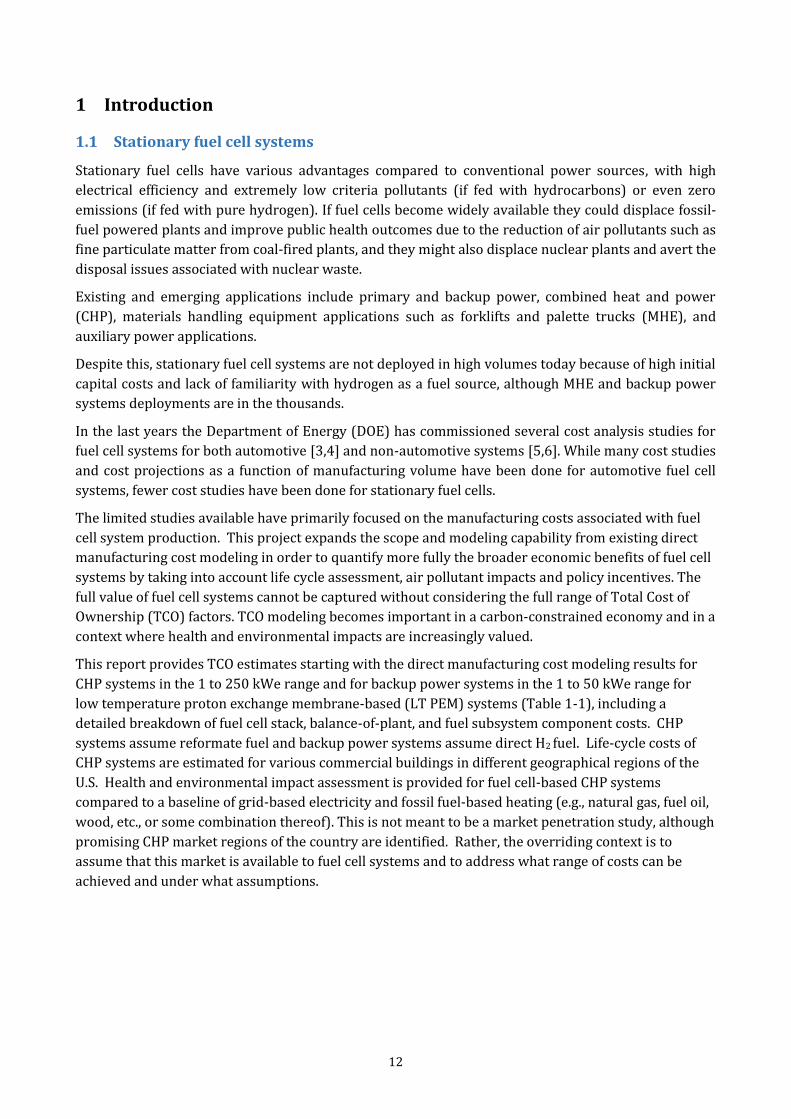
This report provides TCO estimates starting with the direct manufacturing cost modeling results for
CHP systems in the 1 to 250 kWe range and for backup power systems in the 1 to 50 kWe range for
low temperature proton exchange membrane-based (LT PEM) systems (Table 1-1), including a
detailed breakdown of fuel cell stack, balance-of-plant, and fuel subsystem component costs. CHP
systems assume reformate fuel and backup power systems assume direct H2 fuel. Life-cycle costs of
CHP systems are estimated for various commercial buildings in different geographical regions of the
U.S. Health and environmental impact assessment is provided for fuel cell-based CHP systems
compared to a baseline of grid-based electricity and fossil fuel-based heating (e.g., natural gas, fuel oil,
wood, etc., or some combination thereof). This is not meant to be a market penetration study, although
promising CHP market regions of the country are identified. Rather, the overriding context is to
assume that this market is available to fuel cell systems and to address what range of costs can be
achieved and under what assumptions.
13
Table 1-1. Application space for this work. CHP and backup power are studied at various production volumes
and system sizes.
Detailed cost studies provide the basis for estimating cost sensitivities to stack components, materials,
and balance-of-plant components and identify key cost component limiters such as platinum loading.
Other key outputs of this effort are manufacturing cost sensitivities as a function of system size and
annual manufacturing volume. Such studies can help to validate DOE fuel cell system cost targets or
highlight key requirements for DOE targets to be met. Insights gained from this study can be applied
toward the development of lower cost, higher volume-manufacturing processes that can meet DOE
combined heat and power system equipment cost targets.
1.2 Technical Targets and Technical Barriers
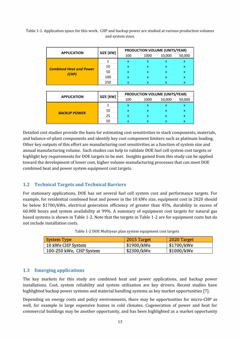
For stationary applications, DOE has set several fuel cell system cost and performance targets. For
example, for residential combined heat and power in the 10 kWe size, equipment cost in 2020 should
be below $1700/kWe, electrical generation efficiency of greater than 45%, durability in excess of
60.000 hours and system availability at 99%. A summary of equipment cost targets for natural gas
based systems is shown in Table 1-2. Note that the targets in Table 1-2 are for equipment costs but do
not include installation costs.
Table 1-2 DOE Multiyear plan system equipment cost targets
1.3 Emerging applications
The key markets for this study are combined heat and power applications, and backup power
installations. Cost, system reliability and system utilization are key drivers. Recent studies have
highlighted backup power systems and material handling systems as key market opportunities [7].
Depending on energy costs and policy environments, there may be opportunities for micro-CHP as
well, for example in large expensive homes in cold climates. Cogeneration of power and heat for
commercial buildings may be another opportunity, and has been highlighted as a market opportunity
100 1000 10,000 50,000
1 x x x x
10 x x x x
50 x x x x
100 x x x x
250 x x x x
APPLICATION SIZE [KW]PRODUCTION VOLUME (UNITS/YEAR)
Combined Heat and Power
(CHP)
100 1000 10,000 50,000
1 x x x x
10 x x x x
25 x x x x
50 x x x x
APPLICATION SIZE [KW]PRODUCTION VOLUME (UNITS/YEAR)
BACKUP POWER
14
for California commercial buildings [6].
Internationally, stationary fuel cell systems are enjoying an increase in interest with programs in
Japan, South Korea and Germany but all markets are still at a cost disadvantage compared to
incumbent technologies. Japan has supported residential fuel cell systems of 0.7-1kWe for co-
generation with generous subsidies, and the recent nuclear reactor accident in Fukishima has
prompted consideration of a range of hydrogen powered systems as alternatives to nuclear energy.
1.4 Total Cost of Ownership Modeling
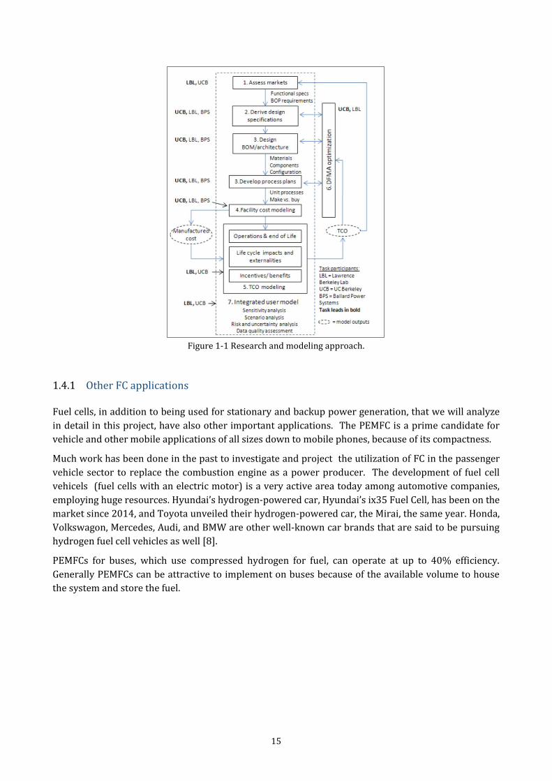
This work estimates the total cost of ownership (TCO) for emerging fuel cell systems manufactured for
stationary applications. The TCO model includes manufacturing costs, operations and end of life
disposition, life cycle impacts, and externality costs and benefits. Other software tools employed
include commercially available Boothroyd Dewhurst DFMA software, existing LCA database tools, and
LBNL exposure and health impact models. The overall research and modeling approach is shown in
Figure 1-1.
The approach for direct manufacturing costs is to utilize Design for Manufacturing and Assembly
(DFMA) techniques to generate system design, materials and manufacturing flow for lowest
manufacturing cost and total cost of ownership. System designs and component costs are developed
and refined based on the following: (1) existing cost studies where applicable; (2) literature and
patent sources; (3) industry and national laboratory advisors.
Life-cycle or use-phase cost modeling utilizes existing characterization of commercial building
electricity and heating demand by geographical region. Life cycle impact assessment (LCIA) is focused
on use-phase impacts from energy use, carbon emissions and pollutant emissions—specifically on
particulate matter (PM) emissions since PM is the dominant contributor to life-cycle health impacts.
Health impact from PM is characterized using existing health impact models available at LBNL. Life-
cycle impact assessment is characterized as a function of fuel cell system adoption by building type
and geographic location. This approach allows the quantification of externalities (e.g. CO2 and
particulate matter) for FC system market adoption in various regions of the U.S.
15
Figure 1-1 Research and modeling approach.
1.4.1 Other FC applications Fuel cells, in addition to being used for stationary and backup power generation, that we will analyze
in detail in this project, have also other important applications. The PEMFC is a prime candidate for
vehicle and other mobile applications of all sizes down to mobile phones, because of its compactness.
Much work has been done in the past to investigate and project the utilization of FC in the passenger
vehicle sector to replace the combustion engine as a power producer. The development of fuel cell
vehicels (fuel cells with an electric motor) is a very active area today among automotive companies,
employing huge resources. Hyundai’s hydrogen-powered car, Hyundai’s ix35 Fuel Cell, has been on the
market since 2014, and Toyota unveiled their hydrogen-powered car, the Mirai, the same year. Honda,
Volkswagon, Mercedes, Audi, and BMW are other well-known car brands that are said to be pursuing
hydrogen fuel cell vehicles as well [8].
PEMFCs for buses, which use compressed hydrogen for fuel, can operate at up to 40% efficiency.
Generally PEMFCs can be attractive to implement on buses because of the available volume to house
the system and store the fuel.
16
2 System Design and Functional Specifications
For this project LTPEM FC system design and functional specifications have been developed for a
range of systems sizes including CHP systems with reformate fuel in the range of 1-250 kW, and
backup power systems from 1kW to 50 kW utilizing direct H2 fuel. These data come from available
data in literature, from industrial specification sheets and from industry advisor inputs.
2.1 CHP System Design
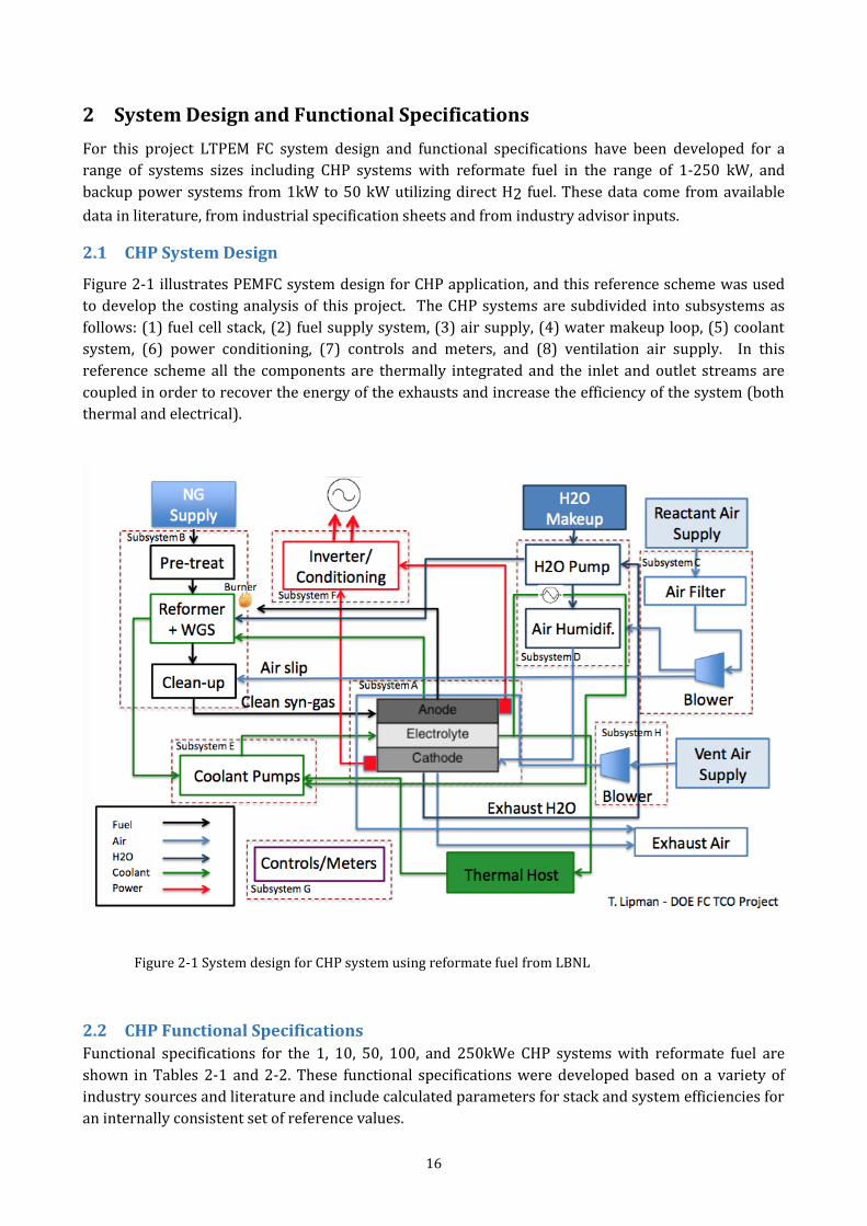
Figure 2-1 illustrates PEMFC system design for CHP application, and this reference scheme was used
to develop the costing analysis of this project. The CHP systems are subdivided into subsystems as
follows: (1) fuel cell stack, (2) fuel supply system, (3) air supply, (4) water makeup loop, (5) coolant
system, (6) power conditioning, (7) controls and meters, and (8) ventilation air supply. In this
reference scheme all the components are thermally integrated and the inlet and outlet streams are
coupled in order to recover the energy of the exhausts and increase the efficiency of the system (both
thermal and electrical).
Figure 2-1 System design for CHP system using reformate fuel from LBNL
2.2 CHP Functional Specifications
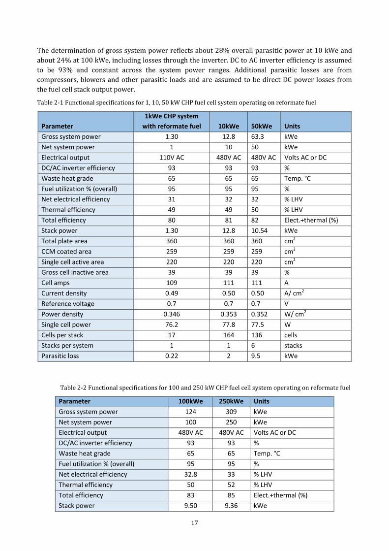
Functional specifications for the 1, 10, 50, 100, and 250kWe CHP systems with reformate fuel are
shown in Tables 2-1 and 2-2. These functional specifications were developed based on a variety of
industry sources and literature and include calculated parameters for stack and system efficiencies for
an internally consistent set of reference values.
17
The determination of gross system power reflects about 28% overall parasitic power at 10 kWe and
about 24% at 100 kWe, including losses through the inverter. DC to AC inverter efficiency is assumed
to be 93% and constant across the system power ranges. Additional parasitic losses are from
compressors, blowers and other parasitic loads and are assumed to be direct DC power losses from
the fuel cell stack output power.
Table 2-1 Functional specifications for 1, 10, 50 kW CHP fuel cell system operating on reformate fuel
Parameter
1kWe CHP system
with reformate fuel 10kWe
50kWe Units
Gross system power 1.30 12.8 63.3 kWe
Net system power 1 10 50 kWe
Electrical output 110V AC 480V AC 480V AC Volts AC or DC
DC/AC inverter efficiency 93 93 93 %
Waste heat grade 65 65 65 Temp. °C
Fuel utilization % (overall) 95 95 95 %
Net electrical efficiency 31 32 32 % LHV
Thermal efficiency 49 49 50 % LHV
Total efficiency 80 81 82 Elect.+thermal (%)
Stack power 1.30 12.8 10.54 kWe
Total plate area 360 360 360 cm2
CCM coated area 259 259 259 cm2
Single cell active area 220 220 220 cm2
Gross cell inactive area 39 39 39 %
Cell amps 109 111 111 A
Current density 0.49 0.50 0.50 A/ cm2
Reference voltage 0.7 0.7 0.7 V
Power density 0.346 0.353 0.352 W/ cm2
Single cell power 76.2 77.8 77.5 W
Cells per stack 17 164 136 cells
Stacks per system 1 1 6 stacks
Parasitic loss 0.22 2 9.5 kWe
Table 2-2 Functional specifications for 100 and 250 kW CHP fuel cell system operating on reformate fuel
Parameter 100kWe 250kWe Units
Gross system power 124 309 kWe
Net system power 100 250 kWe
Electrical output 480V AC 480V AC Volts AC or DC
DC/AC inverter efficiency 93 93 %
Waste heat grade 65 65 Temp. °C
Fuel utilization % (overall) 95 95 %
Net electrical efficiency 32.8 33 % LHV
Thermal efficiency 50 52 % LHV
Total efficiency 83 85 Elect.+thermal (%)
Stack power 9.50 9.36 kWe
18
Total plate area 360 360 cm2
CCM coated area 259 259 cm2
Single cell active area 220 220 cm2
Gross cell inactive area 39 39 %
Cell amps 111 111.4 A
Current density 0.51 0.51 A/ cm2
Reference voltage 0.7 0.7 V
Power density 0.354 0.354 W/ cm2
Single cell power 77.9 78 W
Cells per stack 122 120 cells
Stacks per system 13 33 stacks
Parasitic loss 16.0 40 kWe
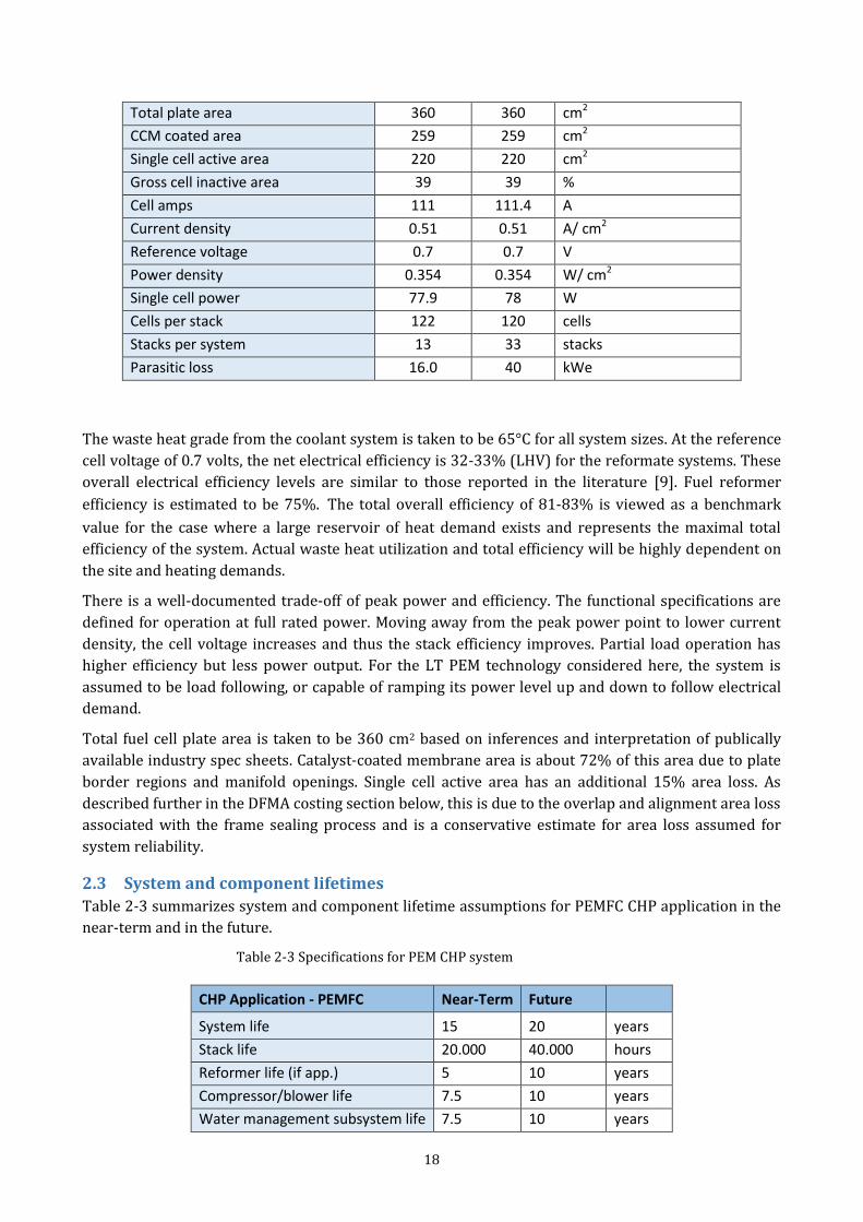
The waste heat grade from the coolant system is taken to be 65°C for all system sizes. At the reference
cell voltage of 0.7 volts, the net electrical efficiency is 32-33% (LHV) for the reformate systems. These
overall electrical efficiency levels are similar to those reported in the literature [9]. Fuel reformer
efficiency is estimated to be 75%.The total overall efficiency of 81-83% is viewed as a benchmark
value for the case where a large reservoir of heat demand exists and represents the maximal total
efficiency of the system. Actual waste heat utilization and total efficiency will be highly dependent on
the site and heating demands.
There is a well-documented trade-off of peak power and efficiency. The functional specifications are
defined for operation at full rated power. Moving away from the peak power point to lower current
density, the cell voltage increases and thus the stack efficiency improves. Partial load operation has
higher efficiency but less power output. For the LT PEM technology considered here, the system is
assumed to be load following, or capable of ramping its power level up and down to follow electrical
demand.
Total fuel cell plate area is taken to be 360 cm2 based on inferences and interpretation of publically
available industry spec sheets. Catalyst-coated membrane area is about 72% of this area due to plate
border regions and manifold openings. Single cell active area has an additional 15% area loss. As
described further in the DFMA costing section below, this is due to the overlap and alignment area loss
associated with the frame sealing process and is a conservative estimate for area loss assumed for
system reliability.
2.3 System and component lifetimes
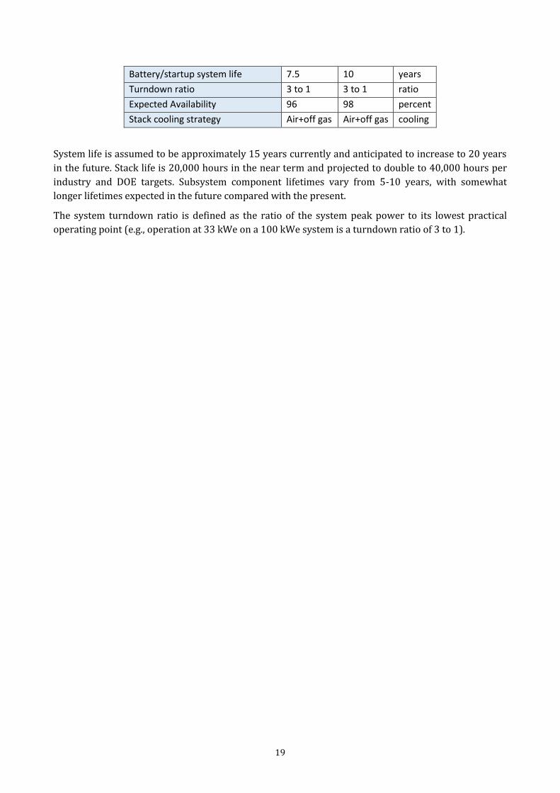
Table 2-3 summarizes system and component lifetime assumptions for PEMFC CHP application in the
near-term and in the future.
Table 2-3 Specifications for PEM CHP system
CHP Application - PEMFC Near-Term Future
System life 15 20 years
Stack life 20.000 40.000 hours
Reformer life (if app.) 5 10 years
Compressor/blower life 7.5 10 years
Water management subsystem life 7.5 10 years
19
Battery/startup system life 7.5 10 years
Turndown ratio 3 to 1 3 to 1 ratio
Expected Availability 96 98 percent
Stack cooling strategy Air+off gas Air+off gas cooling
System life is assumed to be approximately 15 years currently and anticipated to increase to 20 years
in the future. Stack life is 20,000 hours in the near term and projected to double to 40,000 hours per
industry and DOE targets. Subsystem component lifetimes vary from 5-10 years, with somewhat
longer lifetimes expected in the future compared with the present.
The system turndown ratio is defined as the ratio of the system peak power to its lowest practical
operating point (e.g., operation at 33 kWe on a 100 kWe system is a turndown ratio of 3 to 1).
20
3 Costing Approach and Considerations
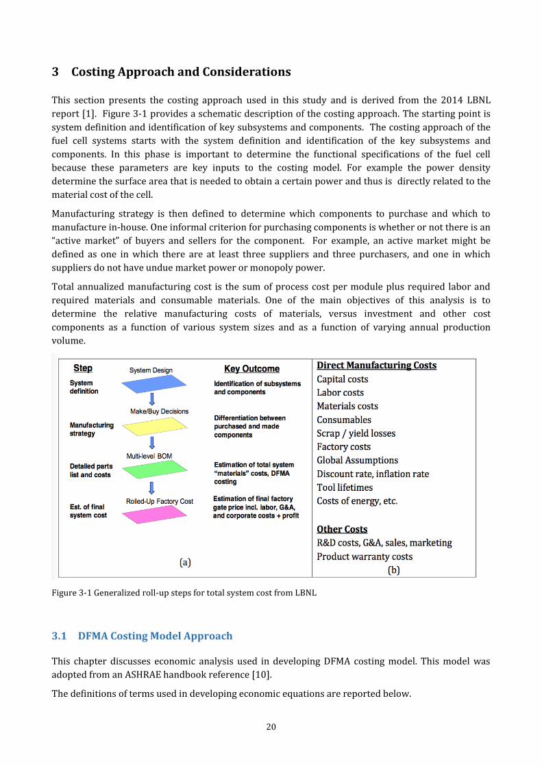
This section presents the costing approach used in this study and is derived from the 2014 LBNL
report [1]. Figure 3-1 provides a schematic description of the costing approach. The starting point is
system definition and identification of key subsystems and components. The costing approach of the
fuel cell systems starts with the system definition and identification of the key subsystems and
components. In this phase is important to determine the functional specifications of the fuel cell
because these parameters are key inputs to the costing model. For example the power density
determine the surface area that is needed to obtain a certain power and thus is directly related to the
material cost of the cell.
Manufacturing strategy is then defined to determine which components to purchase and which to
manufacture in-house. One informal criterion for purchasing components is whether or not there is an
“active market” of buyers and sellers for the component. For example, an active market might be
defined as one in which there are at least three suppliers and three purchasers, and one in which
suppliers do not have undue market power or monopoly power.
Total annualized manufacturing cost is the sum of process cost per module plus required labor and
required materials and consumable materials. One of the main objectives of this analysis is to
determine the relative manufacturing costs of materials, versus investment and other cost
components as a function of various system sizes and as a function of varying annual production
volume.
Figure 3-1 Generalized roll-up steps for total system cost from LBNL
3.1 DFMA Costing Model Approach
This chapter discusses economic analysis used in developing DFMA costing model. This model was
adopted from an ASHRAE handbook reference [10].
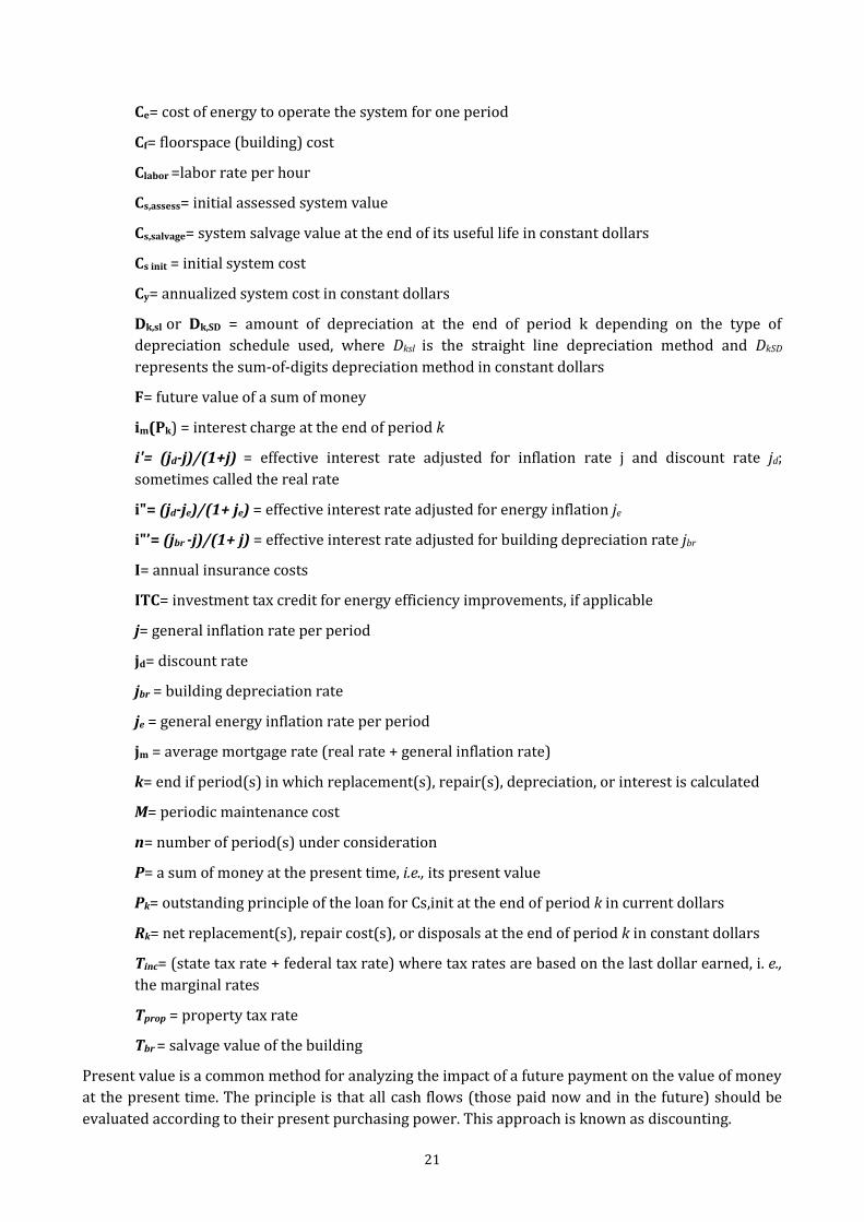
The definitions of terms used in developing economic equations are reported below.
21
Ce= cost of energy to operate the system for one period
Cf= floorspace (building) cost
Clabor =labor rate per hour
Cs,assess= initial assessed system value
Cs,salvage= system salvage value at the end of its useful life in constant dollars
Cs init = initial system cost
Cy= annualized system cost in constant dollars
Dk,sl or Dk,SD = amount of depreciation at the end of period k depending on the type of
depreciation schedule used, where Dksl is the straight line depreciation method and DkSD
represents the sum-of-digits depreciation method in constant dollars
F= future value of a sum of money
im(Pk) = interest charge at the end of period k
i'= (jd-j)/(1+j) = effective interest rate adjusted for inflation rate j and discount rate jd;
sometimes called the real rate
i"= (jd-je)/(1+ je) = effective interest rate adjusted for energy inflation je
i"’= (jbr -j)/(1+ j) = effective interest rate adjusted for building depreciation rate jbr
I= annual insurance costs
ITC= investment tax credit for energy efficiency improvements, if applicable
j= general inflation rate per period
jd= discount rate
jbr = building depreciation rate
je = general energy inflation rate per period
jm = average mortgage rate (real rate + general inflation rate)
k= end if period(s) in which replacement(s), repair(s), depreciation, or interest is calculated
M= periodic maintenance cost
n= number of period(s) under consideration
P= a sum of money at the present time, i.e., its present value
Pk= outstanding principle of the loan for Cs,init at the end of period k in current dollars
Rk= net replacement(s), repair cost(s), or disposals at the end of period k in constant dollars
Tinc= (state tax rate + federal tax rate) where tax rates are based on the last dollar earned, i. e.,
the marginal rates
Tprop = property tax rate
Tbr = salvage value of the building
Present value is a common method for analyzing the impact of a future payment on the value of money
at the present time. The principle is that all cash flows (those paid now and in the future) should be
evaluated according to their present purchasing power. This approach is known as discounting.
22
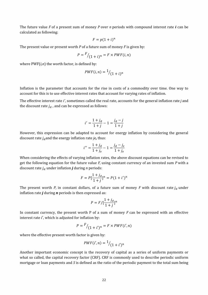
The future value F of a present sum of money P over n periods with compound interest rate i can be
calculated as following:
𝐹 = 𝑝(1 + 𝑖)𝑛
The present value or present worth P of a future sum of money F is given by:
𝑃 = 𝐹(1 + 𝑖)𝑛⁄ = 𝐹 × 𝑃𝑊𝐹(𝑖, 𝑛)
where PWF(i,n) the worth factor, is defined by:
𝑃𝑊𝐹(𝑖, 𝑛) = 1(1 + 𝑖)𝑛⁄
Inflation is the parameter that accounts for the rise in costs of a commodity over time. One way to
account for this is to use effective interest rates that account for varying rates of inflation.
The effective interest rate i', sometimes called the real rate, accounts for the general inflation rate j and
the discount rate 𝑗𝑑 , and can be expressed as follows:
𝑖′ =1 + 𝑗𝑑
1 + 𝑗− 1 =
𝑗𝑑 − 𝑗
1 + 𝑗
However, this expression can be adapted to account for energy inflation by considering the general
discount rate 𝑗𝑑and the energy inflation rate je, thus:
𝑖′′ =1 + 𝑗𝑑
1 + 𝑗𝑒− 1 =
𝑗𝑑 − 𝑗𝑒
1 + 𝑗𝑒
When considering the effects of varying inflation rates, the above discount equations can be revised to
get the following equation for the future value F, using constant currency of an invested sum P with a
discount rate 𝑗𝑑 under inflation j during n periods:
𝐹 = 𝑃[1 + 𝑗𝑑
1 + 𝑗]𝑛 = 𝑃(1 + 𝑖′)𝑛
The present worth P, in constant dollars, of a future sum of money F with discount rate 𝑗𝑑 under
inflation rate j during n periods is then expressed as:
𝑃 = 𝐹/[1 + 𝑗𝑑
1 + 𝑗]𝑛
In constant currency, the present worth P of a sum of money F can be expressed with an effective
interest rate 𝑖′, which is adjusted for inflation by:
𝑃 = 𝐹(1 + 𝑖′)𝑛⁄ = 𝐹 × 𝑃𝑊𝐹(𝑖′, 𝑛)
where the effective present worth factor is given by:
𝑃𝑊𝐹(𝑖′, 𝑛) = 1(1 + 𝑖′)𝑛⁄
Another important economic concept is the recovery of capital as a series of uniform payments or
what so called, the capital recovery factor (CRF). CRF is commonly used to describe periodic uniform
mortgage or loan payments and S is defined as the ratio of the periodic payment to the total sum being
23
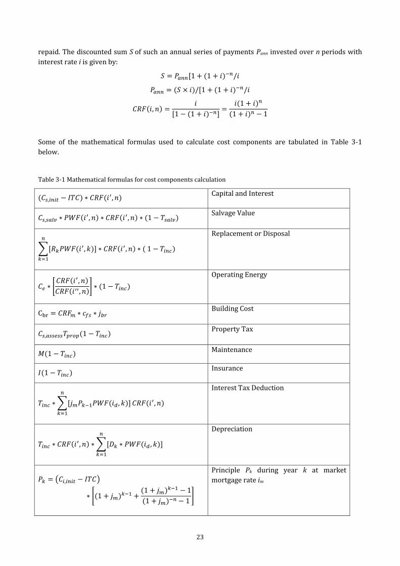
repaid. The discounted sum S of such an annual series of payments Pann invested over n periods with
interest rate i is given by:
𝑆 = 𝑃𝑎𝑛𝑛[1 + (1 + 𝑖)−𝑛/𝑖
𝑃𝑎𝑛𝑛 = (𝑆 × 𝑖)/[1 + (1 + 𝑖)−𝑛/𝑖
𝐶𝑅𝐹(𝑖, 𝑛) =𝑖
[1 − (1 + 𝑖)−𝑛]=
𝑖(1 + 𝑖)𝑛
(1 + 𝑖)𝑛 − 1
Some of the mathematical formulas used to calculate cost components are tabulated in Table 3-1
below.
Table 3-1 Mathematical formulas for cost components calculation
(𝐶𝑠,𝑖𝑛𝑖𝑡 − 𝐼𝑇𝐶) ∗ 𝐶𝑅𝐹(𝑖′, 𝑛) Capital and Interest
𝐶𝑠,𝑠𝑎𝑙𝑣 ∗ 𝑃𝑊𝐹(𝑖′, 𝑛) ∗ 𝐶𝑅𝐹(𝑖′, 𝑛) ∗ (1 − 𝑇𝑠𝑎𝑙𝑣) Salvage Value
∑[𝑅𝑘𝑃𝑊𝐹(𝑖′, 𝑘)]
𝑛
𝑘=1
∗ 𝐶𝑅𝐹(𝑖′, 𝑛) ∗ ( 1 − 𝑇𝑖𝑛𝑐)
Replacement or Disposal
𝐶𝑒 ∗ [𝐶𝑅𝐹(𝑖′, 𝑛)
𝐶𝑅𝐹(𝑖′′, 𝑛)] ∗ (1 − 𝑇𝑖𝑛𝑐)
Operating Energy
Cbr = 𝐶𝑅𝐹𝑚 ∗ 𝑐𝑓𝑠 ∗ 𝑗𝑏𝑟 Building Cost
𝐶𝑠,𝑎𝑠𝑠𝑒𝑠𝑠𝑇𝑝𝑟𝑜𝑝(1 − 𝑇𝑖𝑛𝑐) Property Tax
𝑀(1 − 𝑇𝑖𝑛𝑐) Maintenance
𝐼(1 − 𝑇𝑖𝑛𝑐) Insurance
𝑇𝑖𝑛𝑐 ∗ ∑[𝑗𝑚𝑃𝑘−1𝑃𝑊𝐹(𝑖𝑑 , 𝑘)]
𝑛
𝑘=1
𝐶𝑅𝐹(𝑖′, 𝑛)
Interest Tax Deduction
𝑇𝑖𝑛𝑐 ∗ 𝐶𝑅𝐹(𝑖′, 𝑛) ∗ ∑[𝐷𝑘 ∗ 𝑃𝑊𝐹(𝑖𝑑 , 𝑘)]
𝑛
𝑘=1
Depreciation
𝑃𝑘 = (𝐶𝑖,𝑖𝑛𝑖𝑡 − 𝐼𝑇𝐶)
∗ [(1 + 𝑗𝑚)𝑘−1 +(1 + 𝑗𝑚)𝑘−1 − 1
(1 + 𝑗𝑚)−𝑛 − 1]
Principle Pk during year k at market
mortgage rate im
24
3.2 Parameters for Manufacturing Cost Analysis
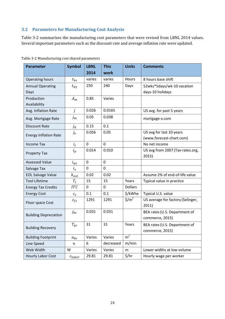
Table 3-2 summarizes the manufacturing cost parameters that were revised from LBNL 2014 values.
Several important parameters such as the discount rate and average inflation rate were updated.
Table 3-2 Manufacturing cost shared parameters
Parameter Symbol LBNL
2014
This
work
Units Comments
Operating hours 𝑡ℎ𝑠 varies varies Hours 8 hours base shift
Annual Operating
Days
𝑡𝑑𝑦 250 240 Days 52wks*5days/wk-10 vacation
days-10 holidays
Production
Availability
𝐴𝑚 0.85 Varies
Avg. Inflation Rate 𝑗 0.026 0.0165 US avg. for past 5 years
Avg. Mortgage Rate 𝑗𝑚 0.05 0.038 mortgage-x.com
Discount Rate 𝑗𝑑 0.15 0.1
Energy Inflation Rate 𝑗𝑒 0.056 0.05 US avg for last 10 years
(www.forecast-chart.com)
Income Tax 𝑖𝑖 0 0 No net income
Property Tax 𝑖𝑝 0.014 0.010 US avg from 2007 (Tax-rates.org,
2015)
Assessed Value 𝑖𝑎𝑣 0 0
Salvage Tax 𝑖𝑠 0 0
EOL Salvage Value 𝑘𝑒𝑜𝑙 0.02 0.02 Assume 2% of end-of-life value
Tool Lifetime 𝑇𝑡 15 15 Years Typical value in practice
Energy Tax Credits 𝐼𝑇𝐶 0 0 Dollars
Energy Cost 𝑐𝑒 0.1 0.1 $/kWhe Typical U.S. value
Floor space Cost 𝑐𝑓𝑠 1291 1291 $/m2 US average for factory (Selinger,
2011)
Building Depreciation 𝑗𝑏𝑟 0.031 0.031 BEA rates (U.S. Department of
commerce, 2015)
Building Recovery 𝑇𝑏𝑟 31 31 Years BEA rates (U.S. Department of
commerce, 2015)
Building Footprint 𝑎𝑏𝑟 Varies Varies m2
Line Speed vl 6 decreased m/min
Web Width W Varies Varies m Lower widths at low volume
Hourly Labor Cost 𝑐𝑙𝑎𝑏𝑜𝑟 29.81 29.81 $/hr Hourly wage per worker
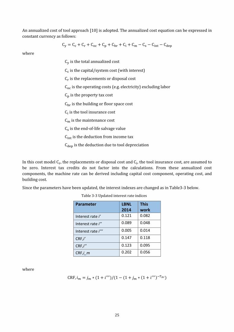
25
An annualized cost of tool approach [10] is adopted. The annualized cost equation can be expressed in
constant currency as follows:
Cy = Cc + Cr + Coc + Cp + Cbr + Ci + Cm − Cs − Cint − Cdep
where
Cy is the total annualized cost
Cc is the capital/system cost (with interest)
Cr is the replacements or disposal cost
Coc is the operating costs (e.g. electricity) excluding labor
Cp is the property tax cost
Cbr is the building or floor space cost
Ci is the tool insurance cost
Cm is the maintenance cost
Cs is the end-of-life salvage value
Cint is the deduction from income tax
Cdep is the deduction due to tool depreciation
In this cost model Cr, the replacements or disposal cost and Ci, the tool insurance cost, are assumed to
be zero. Interest tax credits do not factor into the calculations. From these annualized cost
components, the machine rate can be derived including capital cost component, operating cost, and
building cost.
Since the parameters have been updated, the interest indexes are changed as in Table3-3 below.
Table 3-3 Updated interest rate indices
Parameter LBNL 2014
This work
Interest rate i’ 0.121 0.082
Interest rate i’’ 0.089 0.048
Interest rate i’’’ 0.005 0.014
CRF,i’ 0.147 0.118
CRF,i’’ 0.123 0.095
CRF,i_m 0.202 0.056
where
CRF, 𝑖𝑚 = 𝑗𝑚 ∗ (1 + 𝑖′′′)/(1 − (1 + 𝑗𝑚 ∗ (1 + 𝑖′′′)−𝑇𝑏𝑟)
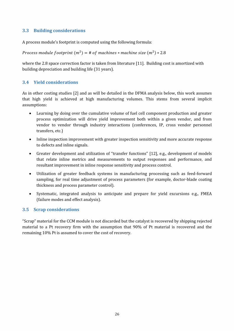
26
3.3 Building considerations
A process module’s footprint is computed using the following formula:
𝑃𝑟𝑜𝑐𝑒𝑠𝑠 𝑚𝑜𝑑𝑢𝑙𝑒 𝑓𝑜𝑜𝑡𝑝𝑟𝑖𝑛𝑡 (𝑚2) = # 𝑜𝑓 𝑚𝑎𝑐ℎ𝑖𝑛𝑒𝑠 ∗ 𝑚𝑎𝑐ℎ𝑖𝑛𝑒 𝑠𝑖𝑧𝑒 (𝑚2) ∗ 2.8
where the 2.8 space correction factor is taken from literature [11]. Building cost is amortized with
building depreciation and building life (31 years).
3.4 Yield considerations
As in other costing studies [2] and as will be detailed in the DFMA analysis below, this work assumes
that high yield is achieved at high manufacturing volumes. This stems from several implicit
assumptions:
Learning by doing over the cumulative volume of fuel cell component production and greater
process optimization will drive yield improvement both within a given vendor, and from
vendor to vendor through industry interactions (conferences, IP, cross vendor personnel
transfers, etc.)
Inline inspection improvement with greater inspection sensitivity and more accurate response
to defects and inline signals.
Greater development and utilization of “transfer functions” [12], e.g., development of models
that relate inline metrics and measurements to output responses and performance, and
resultant improvement in inline response sensitivity and process control.
Utilization of greater feedback systems in manufacturing processing such as feed-forward
sampling, for real time adjustment of process parameters (for example, doctor-blade coating
thickness and process parameter control).
Systematic, integrated analysis to anticipate and prepare for yield excursions e.g., FMEA
(failure modes and effect analysis).
3.5 Scrap considerations
“Scrap” material for the CCM module is not discarded but the catalyst is recovered by shipping rejected
material to a Pt recovery firm with the assumption that 90% of Pt material is recovered and the
remaining 10% Pt is assumed to cover the cost of recovery.
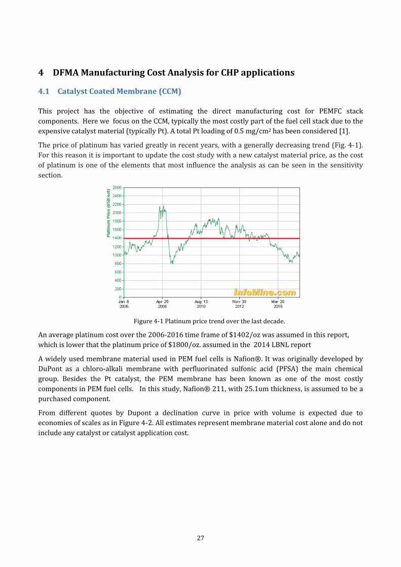
27
4 DFMA Manufacturing Cost Analysis for CHP applications
4.1 Catalyst Coated Membrane (CCM)
This project has the objective of estimating the direct manufacturing cost for PEMFC stack
components. Here we focus on the CCM, typically the most costly part of the fuel cell stack due to the
expensive catalyst material (typically Pt). A total Pt loading of 0.5 mg/cm2 has been considered [1].
The price of platinum has varied greatly in recent years, with a generally decreasing trend (Fig. 4-1).
For this reason it is important to update the cost study with a new catalyst material price, as the cost
of platinum is one of the elements that most influence the analysis as can be seen in the sensitivity
section.
Figure 4-1 Platinum price trend over the last decade.
An average platinum cost over the 2006-2016 time frame of $1402/oz was assumed in this report,
which is lower that the platinum price of $1800/oz. assumed in the 2014 LBNL report
A widely used membrane material used in PEM fuel cells is Nafion®. It was originally developed by
DuPont as a chloro‐alkali membrane with perfluorinated sulfonic acid (PFSA) the main chemical
group. Besides the Pt catalyst, the PEM membrane has been known as one of the most costly
components in PEM fuel cells. In this study, Nafion® 211, with 25.1um thickness, is assumed to be a
purchased component.
From different quotes by Dupont a declination curve in price with volume is expected due to
economies of scales as in Figure 4-2. All estimates represent membrane material cost alone and do not
include any catalyst or catalyst application cost.
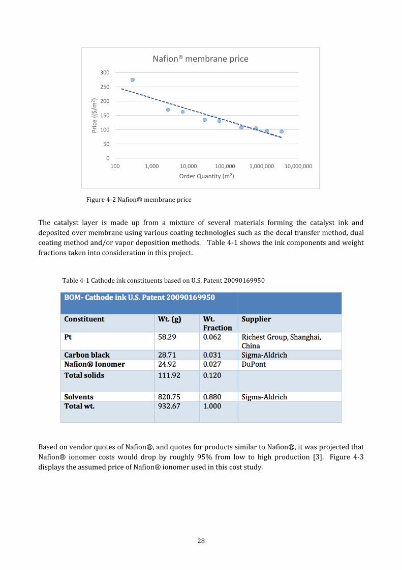
28
Figure 4-2 Nafion® membrane price
The catalyst layer is made up from a mixture of several materials forming the catalyst ink and
deposited over membrane using various coating technologies such as the decal transfer method, dual
coating method and/or vapor deposition methods. Table 4-1 shows the ink components and weight
fractions taken into consideration in this project.
Table 4-1 Cathode ink constituents based on U.S. Patent 20090169950
Based on vendor quotes of Nafion®, and quotes for products similar to Nafion®, it was projected that
Nafion® ionomer costs would drop by roughly 95% from low to high production [3]. Figure 4-3
displays the assumed price of Nafion® ionomer used in this cost study.
0
50
100
150
200
250
300
100 1,000 10,000 100,000 1,000,000 10,000,000
Pri
ce (
($/m
2 )
Order Quantity (m2)
Nafion® membrane price
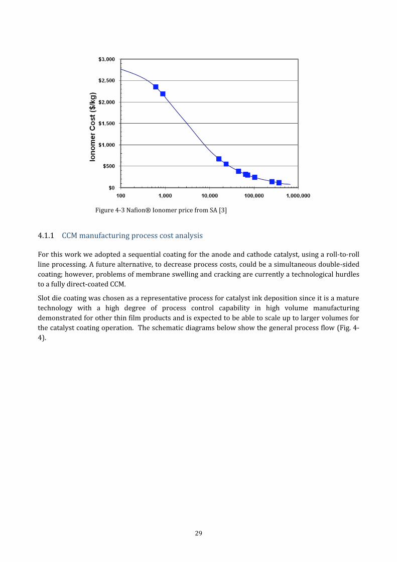
29
Figure 4-3 Nafion® Ionomer price from SA [3]
4.1.1 CCM manufacturing process cost analysis For this work we adopted a sequential coating for the anode and cathode catalyst, using a roll-to-roll
line processing. A future alternative, to decrease process costs, could be a simultaneous double-sided
coating; however, problems of membrane swelling and cracking are currently a technological hurdles
to a fully direct-coated CCM.
Slot die coating was chosen as a representative process for catalyst ink deposition since it is a mature
technology with a high degree of process control capability in high volume manufacturing
demonstrated for other thin film products and is expected to be able to scale up to larger volumes for
the catalyst coating operation. The schematic diagrams below show the general process flow (Fig. 4-
4).
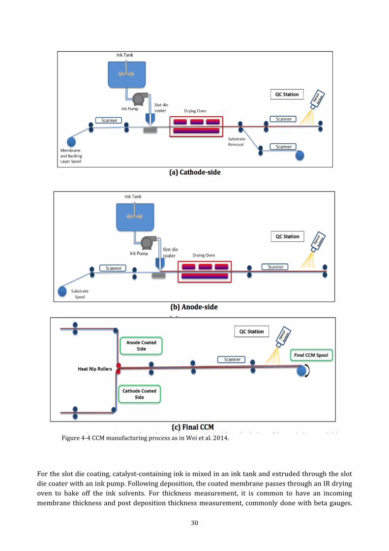
30
Figure 4-4 CCM manufacturing process as in Wei et al. 2014.
For the slot die coating, catalyst-containing ink is mixed in an ink tank and extruded through the slot
die coater with an ink pump. Following deposition, the coated membrane passes through an IR drying
oven to bake off the ink solvents. For thickness measurement, it is common to have an incoming
membrane thickness and post deposition thickness measurement, commonly done with beta gauges.
31
The overall deposition area is enclosed in a clean room environment at Class 1000 to control for
contaminants and particles. An inspection is done after each deposition and thermal treatment pass.
4.1.1.1 CCM Manufacturing line process parameters
Ideally, the equipment should run at its required rate and make good quality products. In practice,
downtime occurs or substandard-quality products are made. These losses, caused by machine
malfunctioning and process errors and defects, can be divided into []:
• Down time losses: when the machine should run, but stands unutilized. Most common down‐time
losses happen when a malfunction arises, or unplanned maintenance tasks must be done in addition to
the major planned upgrades or set-up/start-up activities.
• Speed losses: the equipment is running, but it is not running at its maximum designed speed. Most
common speed losses happen when equipment speed decrease but is not at zero. These losses can
arise from equipment malfunctioning, small technical imperfections, such as stuck packaging or
because of the start-up of the equipment related to a maintenance task, setup issues or a stop for
organizational reasons.
• Quality losses: the equipment is producing products that do not fully meet the specified quality
requirements. Most common quality losses occur because equipment, in the time between start-up
and completely stable operation, yields products that do not conform to quality demand. They may
occure due to incorrect functioning of the machine or because process parameters are not tuned to
optimal processing conditions.
These losses can be considered using three different measurable components [19]:
1. Availability, the percentage of time that equipment is available to run during the total possible
planned production up-time
2. Line Performance, the measure of how well the machine runs within target operating times.
3. Process Yield, the measure of the number of parts that meet specification compared to how
many were produced
Process yield and line availability are both functions of annual production volume since level of
automation and number of manufacturing lines increase with volume. Under these assumptions, line
availability is assumed to be 80% and process yield to be 85% at low volumes (<100.000 units/year).
At the highest volumes (>10.000.000 units/year), line availability and process yield are estimated to
be 95%. For volumes between 100.000 and 10.000.000 units/year, the process parameters are found
through exponential interpolation.
Line performance is assumed to be 89% for manual configuration and 95% for semi automatic and
automatic configurations [14]. The process parameters are shown in Table 4-2.
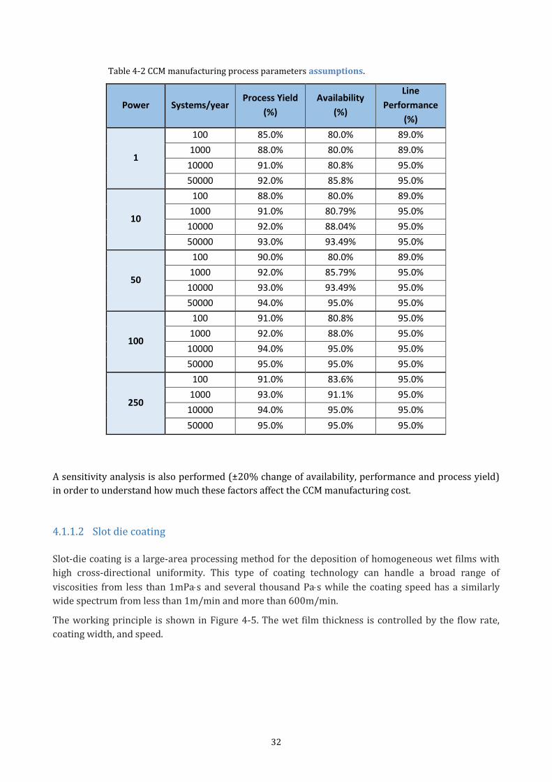
32
Table 4-2 CCM manufacturing process parameters assumptions.
Power Systems/year Process Yield
(%)
Availability
(%)
Line
Performance
(%)
1
100 85.0% 80.0% 89.0%
1000 88.0% 80.0% 89.0%
10000 91.0% 80.8% 95.0%
50000 92.0% 85.8% 95.0%
10
100 88.0% 80.0% 89.0%
1000 91.0% 80.79% 95.0%
10000 92.0% 88.04% 95.0%
50000 93.0% 93.49% 95.0%
50
100 90.0% 80.0% 89.0%
1000 92.0% 85.79% 95.0%
10000 93.0% 93.49% 95.0%
50000 94.0% 95.0% 95.0%
100
100 91.0% 80.8% 95.0%
1000 92.0% 88.0% 95.0%
10000 94.0% 95.0% 95.0%
50000 95.0% 95.0% 95.0%
250
100 91.0% 83.6% 95.0%
1000 93.0% 91.1% 95.0%
10000 94.0% 95.0% 95.0%
50000 95.0% 95.0% 95.0%
A sensitivity analysis is also performed (±20% change of availability, performance and process yield)
in order to understand how much these factors affect the CCM manufacturing cost.
4.1.1.2 Slot die coating
Slot-die coating is a large-area processing method for the deposition of homogeneous wet films with
high cross-directional uniformity. This type of coating technology can handle a broad range of
viscosities from less than 1mPas and several thousand Pas while the coating speed has a similarly
wide spectrum from less than 1m/min and more than 600m/min.
The working principle is shown in Figure 4-5. The wet film thickness is controlled by the flow rate,
coating width, and speed.
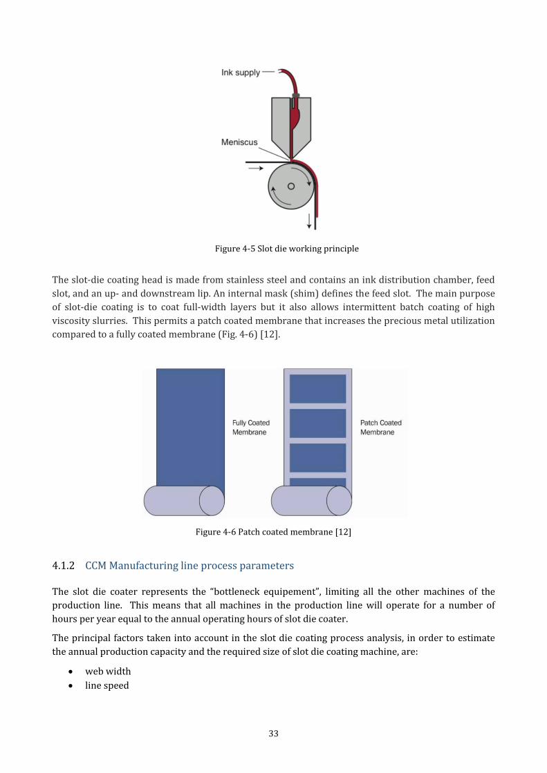
33
Figure 4-5 Slot die working principle
The slot-die coating head is made from stainless steel and contains an ink distribution chamber, feed
slot, and an up- and downstream lip. An internal mask (shim) defines the feed slot. The main purpose
of slot-die coating is to coat full-width layers but it also allows intermittent batch coating of high
viscosity slurries. This permits a patch coated membrane that increases the precious metal utilization
compared to a fully coated membrane (Fig. 4-6) [12].
Figure 4-6 Patch coated membrane [12]
4.1.2 CCM Manufacturing line process parameters The slot die coater represents the “bottleneck equipement”, limiting all the other machines of the
production line. This means that all machines in the production line will operate for a number of
hours per year equal to the annual operating hours of slot die coater.
The principal factors taken into account in the slot die coating process analysis, in order to estimate
the annual production capacity and the required size of slot die coating machine, are:
web width
line speed
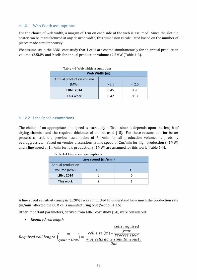
34
4.1.2.1 Web Width assumptions
For the choice of web width, a margin of 1cm on each side of the web is assumed. Since the slot die
coater can be manufactured at any desired width, this dimension is calculated based on the number of
pieces made simultaneously.
We assume, as in the LBNL cost study that 4 cells are coated simultaneously for an annual production
volume <2.5MW and 9 cells for annual production volume >2.5MW (Table 4-3).
Table 4-3 Web width assumptions
Web Width (m)
Annual production volume
(MW) > 2.5 < 2.5
LBNL 2014 0.45 0.90
This work 0.42 0.92
4.1.2.2 Line Speed assumptions
The choice of an appropriate line speed is extremely difficult since it depends upon the length of
drying chamber and the required thickness of the ink used [15]. For these reasons and for better
process control, the previous assumption of 6m/min for all production volumes is probably
overaggressive. Based on vendor discussions, a line speed of 2m/min for high production (>1MW)
and a line speed of 1m/min for low production (<1MW) are assumed for this work (Table 4-4).
Table 4-4 Line speed assumptions
Line speed (m/min)
Annual production
volume (MW) > 1 < 1
LBNL 2014 6 6
This work 2 1
A line speed sensitivity analysis (±20%) was conducted to understand how much the production rate
(m/min) affected the CCM cells manufacturing cost (Section 4.1.5).
Other important parameters, derived from LBNL cost study [14], were considered:
Required roll length
𝑅𝑒𝑞𝑢𝑖𝑟𝑒𝑑 𝑟𝑜𝑙𝑙 𝑙𝑒𝑛𝑔𝑡ℎ (𝑚
𝑦𝑒𝑎𝑟 ∗ 𝑙𝑖𝑛𝑒) =
𝑐𝑒𝑙𝑙 𝑠𝑖𝑧𝑒 (𝑚) ∗
𝑐𝑒𝑙𝑙𝑠 𝑟𝑒𝑞𝑢𝑖𝑟𝑒𝑑𝑦𝑒𝑎𝑟
𝑃𝑟𝑜𝑐𝑒𝑠𝑠 𝑌𝑖𝑒𝑙𝑑# 𝑜𝑓 𝑐𝑒𝑙𝑙𝑠 𝑑𝑜𝑛𝑒 𝑠𝑖𝑚𝑢𝑙𝑡𝑎𝑛𝑒𝑜𝑢𝑠𝑙𝑦
𝑙𝑖𝑛𝑒
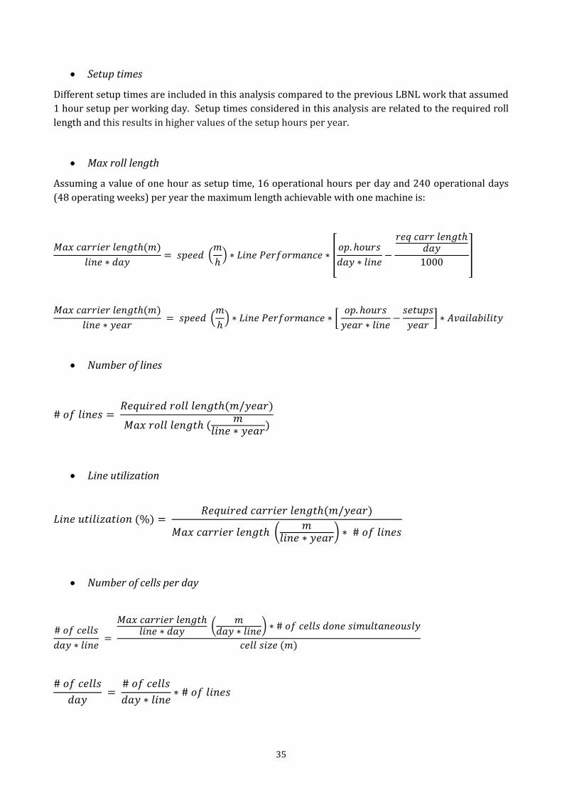
35
Setup times
Different setup times are included in this analysis compared to the previous LBNL work that assumed
1 hour setup per working day. Setup times considered in this analysis are related to the required roll
length and this results in higher values of the setup hours per year.
Max roll length
Assuming a value of one hour as setup time, 16 operational hours per day and 240 operational days
(48 operating weeks) per year the maximum length achievable with one machine is:
𝑀𝑎𝑥 𝑐𝑎𝑟𝑟𝑖𝑒𝑟 𝑙𝑒𝑛𝑔𝑡ℎ(𝑚)
𝑙𝑖𝑛𝑒 ∗ 𝑑𝑎𝑦= 𝑠𝑝𝑒𝑒𝑑 (
𝑚
ℎ) ∗ 𝐿𝑖𝑛𝑒 𝑃𝑒𝑟𝑓𝑜𝑟𝑚𝑎𝑛𝑐𝑒 ∗ [
𝑜𝑝. ℎ𝑜𝑢𝑟𝑠
𝑑𝑎𝑦 ∗ 𝑙𝑖𝑛𝑒−
𝑟𝑒𝑞 𝑐𝑎𝑟𝑟 𝑙𝑒𝑛𝑔𝑡ℎ𝑑𝑎𝑦
1000]
𝑀𝑎𝑥 𝑐𝑎𝑟𝑟𝑖𝑒𝑟 𝑙𝑒𝑛𝑔𝑡ℎ(𝑚)
𝑙𝑖𝑛𝑒 ∗ 𝑦𝑒𝑎𝑟 = 𝑠𝑝𝑒𝑒𝑑 (
𝑚
ℎ) ∗ 𝐿𝑖𝑛𝑒 𝑃𝑒𝑟𝑓𝑜𝑟𝑚𝑎𝑛𝑐𝑒 ∗ [
𝑜𝑝. ℎ𝑜𝑢𝑟𝑠
𝑦𝑒𝑎𝑟 ∗ 𝑙𝑖𝑛𝑒−
𝑠𝑒𝑡𝑢𝑝𝑠
𝑦𝑒𝑎𝑟] ∗ 𝐴𝑣𝑎𝑖𝑙𝑎𝑏𝑖𝑙𝑖𝑡𝑦
Number of lines
# 𝑜𝑓 𝑙𝑖𝑛𝑒𝑠 = 𝑅𝑒𝑞𝑢𝑖𝑟𝑒𝑑 𝑟𝑜𝑙𝑙 𝑙𝑒𝑛𝑔𝑡ℎ(𝑚/𝑦𝑒𝑎𝑟)
𝑀𝑎𝑥 𝑟𝑜𝑙𝑙 𝑙𝑒𝑛𝑔𝑡ℎ (𝑚
𝑙𝑖𝑛𝑒 ∗ 𝑦𝑒𝑎𝑟)
Line utilization
𝐿𝑖𝑛𝑒 𝑢𝑡𝑖𝑙𝑖𝑧𝑎𝑡𝑖𝑜𝑛 (%) = 𝑅𝑒𝑞𝑢𝑖𝑟𝑒𝑑 𝑐𝑎𝑟𝑟𝑖𝑒𝑟 𝑙𝑒𝑛𝑔𝑡ℎ(𝑚/𝑦𝑒𝑎𝑟)
𝑀𝑎𝑥 𝑐𝑎𝑟𝑟𝑖𝑒𝑟 𝑙𝑒𝑛𝑔𝑡ℎ (𝑚
𝑙𝑖𝑛𝑒 ∗ 𝑦𝑒𝑎𝑟) ∗ # 𝑜𝑓 𝑙𝑖𝑛𝑒𝑠
Number of cells per day
# 𝑜𝑓 𝑐𝑒𝑙𝑙𝑠
𝑑𝑎𝑦 ∗ 𝑙𝑖𝑛𝑒 =
𝑀𝑎𝑥 𝑐𝑎𝑟𝑟𝑖𝑒𝑟 𝑙𝑒𝑛𝑔𝑡ℎ𝑙𝑖𝑛𝑒 ∗ 𝑑𝑎𝑦
(𝑚
𝑑𝑎𝑦 ∗ 𝑙𝑖𝑛𝑒) ∗ # 𝑜𝑓 𝑐𝑒𝑙𝑙𝑠 𝑑𝑜𝑛𝑒 𝑠𝑖𝑚𝑢𝑙𝑡𝑎𝑛𝑒𝑜𝑢𝑠𝑙𝑦
𝑐𝑒𝑙𝑙 𝑠𝑖𝑧𝑒 (𝑚)
# 𝑜𝑓 𝑐𝑒𝑙𝑙𝑠
𝑑𝑎𝑦 =
# 𝑜𝑓 𝑐𝑒𝑙𝑙𝑠
𝑑𝑎𝑦 ∗ 𝑙𝑖𝑛𝑒∗ # 𝑜𝑓 𝑙𝑖𝑛𝑒𝑠
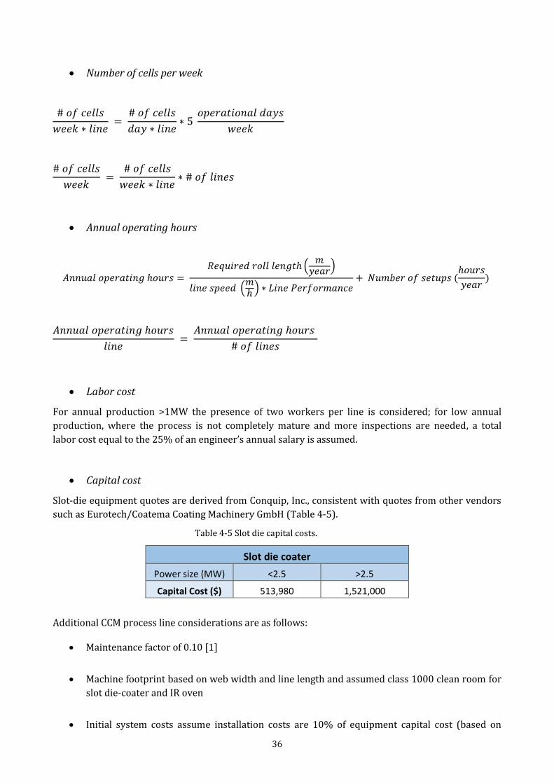
36
Number of cells per week
# 𝑜𝑓 𝑐𝑒𝑙𝑙𝑠
𝑤𝑒𝑒𝑘 ∗ 𝑙𝑖𝑛𝑒 =
# 𝑜𝑓 𝑐𝑒𝑙𝑙𝑠
𝑑𝑎𝑦 ∗ 𝑙𝑖𝑛𝑒∗ 5
𝑜𝑝𝑒𝑟𝑎𝑡𝑖𝑜𝑛𝑎𝑙 𝑑𝑎𝑦𝑠
𝑤𝑒𝑒𝑘
# 𝑜𝑓 𝑐𝑒𝑙𝑙𝑠
𝑤𝑒𝑒𝑘 =
# 𝑜𝑓 𝑐𝑒𝑙𝑙𝑠
𝑤𝑒𝑒𝑘 ∗ 𝑙𝑖𝑛𝑒∗ # 𝑜𝑓 𝑙𝑖𝑛𝑒𝑠
Annual operating hours
𝐴𝑛𝑛𝑢𝑎𝑙 𝑜𝑝𝑒𝑟𝑎𝑡𝑖𝑛𝑔 ℎ𝑜𝑢𝑟𝑠 = 𝑅𝑒𝑞𝑢𝑖𝑟𝑒𝑑 𝑟𝑜𝑙𝑙 𝑙𝑒𝑛𝑔𝑡ℎ (
𝑚𝑦𝑒𝑎𝑟)
𝑙𝑖𝑛𝑒 𝑠𝑝𝑒𝑒𝑑 (𝑚ℎ
) ∗ 𝐿𝑖𝑛𝑒 𝑃𝑒𝑟𝑓𝑜𝑟𝑚𝑎𝑛𝑐𝑒+ 𝑁𝑢𝑚𝑏𝑒𝑟 𝑜𝑓 𝑠𝑒𝑡𝑢𝑝𝑠 (
ℎ𝑜𝑢𝑟𝑠
𝑦𝑒𝑎𝑟)
𝐴𝑛𝑛𝑢𝑎𝑙 𝑜𝑝𝑒𝑟𝑎𝑡𝑖𝑛𝑔 ℎ𝑜𝑢𝑟𝑠
𝑙𝑖𝑛𝑒 =
𝐴𝑛𝑛𝑢𝑎𝑙 𝑜𝑝𝑒𝑟𝑎𝑡𝑖𝑛𝑔 ℎ𝑜𝑢𝑟𝑠
# 𝑜𝑓 𝑙𝑖𝑛𝑒𝑠
Labor cost
For annual production >1MW the presence of two workers per line is considered; for low annual
production, where the process is not completely mature and more inspections are needed, a total
labor cost equal to the 25% of an engineer’s annual salary is assumed.
Capital cost
Slot-die equipment quotes are derived from Conquip, Inc., consistent with quotes from other vendors
such as Eurotech/Coatema Coating Machinery GmbH (Table 4-5).
Table 4-5 Slot die capital costs.
Slot die coater
Power size (MW) <2.5 >2.5
Capital Cost ($) 513,980 1,521,000
Additional CCM process line considerations are as follows:
Maintenance factor of 0.10 [1]
Machine footprint based on web width and line length and assumed class 1000 clean room for
slot die-coater and IR oven
Initial system costs assume installation costs are 10% of equipment capital cost (based on
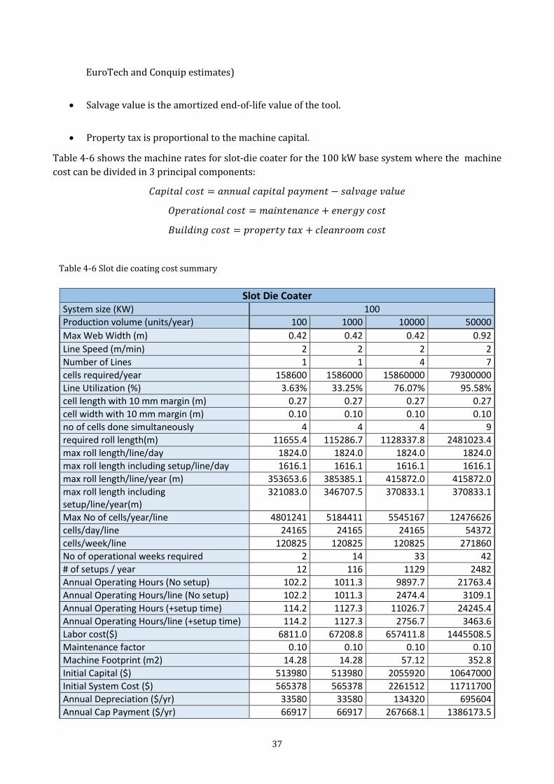
37
EuroTech and Conquip estimates)
Salvage value is the amortized end-of-life value of the tool.
Property tax is proportional to the machine capital.
Table 4-6 shows the machine rates for slot-die coater for the 100 kW base system where the machine
cost can be divided in 3 principal components:
𝐶𝑎𝑝𝑖𝑡𝑎𝑙 𝑐𝑜𝑠𝑡 = 𝑎𝑛𝑛𝑢𝑎𝑙 𝑐𝑎𝑝𝑖𝑡𝑎𝑙 𝑝𝑎𝑦𝑚𝑒𝑛𝑡 − 𝑠𝑎𝑙𝑣𝑎𝑔𝑒 𝑣𝑎𝑙𝑢𝑒
𝑂𝑝𝑒𝑟𝑎𝑡𝑖𝑜𝑛𝑎𝑙 𝑐𝑜𝑠𝑡 = 𝑚𝑎𝑖𝑛𝑡𝑒𝑛𝑎𝑛𝑐𝑒 + 𝑒𝑛𝑒𝑟𝑔𝑦 𝑐𝑜𝑠𝑡
𝐵𝑢𝑖𝑙𝑑𝑖𝑛𝑔 𝑐𝑜𝑠𝑡 = 𝑝𝑟𝑜𝑝𝑒𝑟𝑡𝑦 𝑡𝑎𝑥 + 𝑐𝑙𝑒𝑎𝑛𝑟𝑜𝑜𝑚 𝑐𝑜𝑠𝑡
Table 4-6 Slot die coating cost summary
Slot Die Coater
System size (KW) 100
Production volume (units/year) 100 1000 10000 50000
Max Web Width (m) 0.42 0.42 0.42 0.92
Line Speed (m/min) 2 2 2 2
Number of Lines 1 1 4 7
cells required/year 158600 1586000 15860000 79300000
Line Utilization (%) 3.63% 33.25% 76.07% 95.58%
cell length with 10 mm margin (m) 0.27 0.27 0.27 0.27
cell width with 10 mm margin (m) 0.10 0.10 0.10 0.10
no of cells done simultaneously 4 4 4 9
required roll length(m) 11655.4 115286.7 1128337.8 2481023.4
max roll length/line/day 1824.0 1824.0 1824.0 1824.0
max roll length including setup/line/day 1616.1 1616.1 1616.1 1616.1
max roll length/line/year (m) 353653.6 385385.1 415872.0 415872.0
max roll length including setup/line/year(m)
321083.0 346707.5 370833.1 370833.1
Max No of cells/year/line 4801241 5184411 5545167 12476626
cells/day/line 24165 24165 24165 54372
cells/week/line 120825 120825 120825 271860
No of operational weeks required 2 14 33 42
# of setups / year 12 116 1129 2482
Annual Operating Hours (No setup) 102.2 1011.3 9897.7 21763.4
Annual Operating Hours/line (No setup) 102.2 1011.3 2474.4 3109.1
Annual Operating Hours (+setup time) 114.2 1127.3 11026.7 24245.4
Annual Operating Hours/line (+setup time) 114.2 1127.3 2756.7 3463.6
Labor cost($) 6811.0 67208.8 657411.8 1445508.5
Maintenance factor 0.10 0.10 0.10 0.10
Machine Footprint (m2) 14.28 14.28 57.12 352.8
Initial Capital ($) 513980 513980 2055920 10647000
Initial System Cost ($) 565378 565378 2261512 11711700
Annual Depreciation ($/yr) 33580 33580 134320 695604
Annual Cap Payment ($/yr) 66917 66917 267668.1 1386173.5
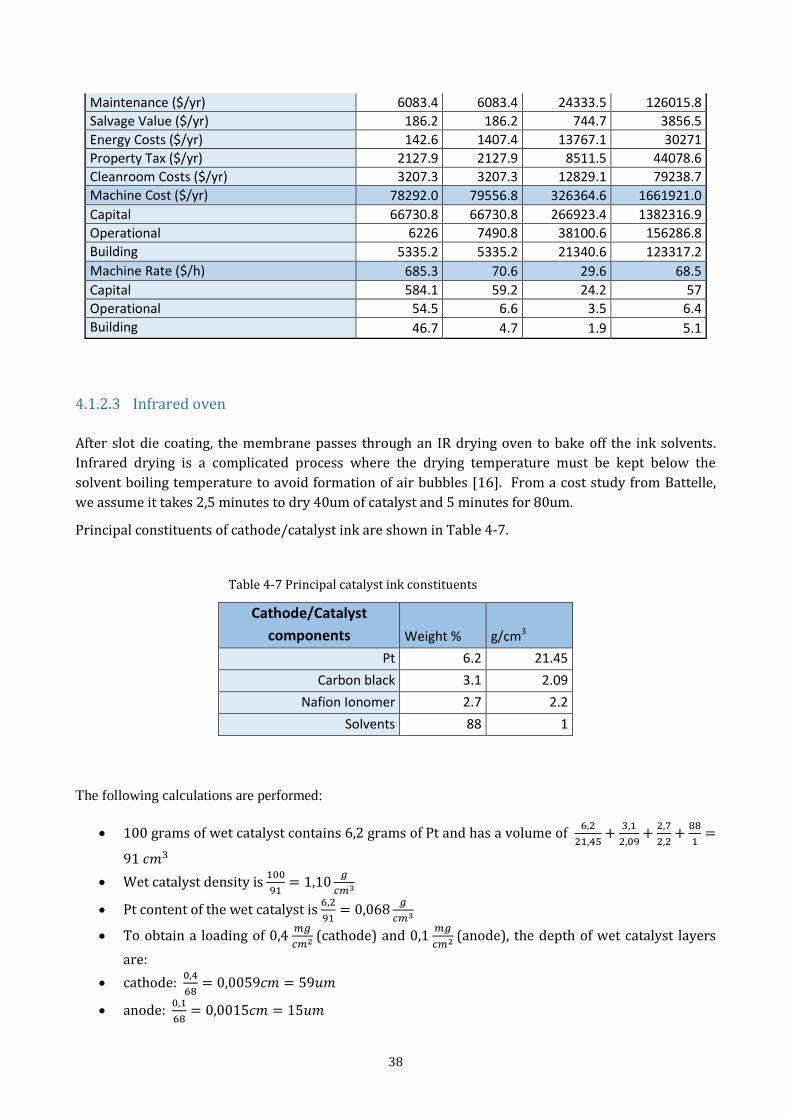
38
Maintenance ($/yr) 6083.4 6083.4 24333.5 126015.8
Salvage Value ($/yr) 186.2 186.2 744.7 3856.5
Energy Costs ($/yr) 142.6 1407.4 13767.1 30271
Property Tax ($/yr) 2127.9 2127.9 8511.5 44078.6
Cleanroom Costs ($/yr) 3207.3 3207.3 12829.1 79238.7
Machine Cost ($/yr) 78292.0 79556.8 326364.6 1661921.0
Capital 66730.8 66730.8 266923.4 1382316.9
Operational 6226 7490.8 38100.6 156286.8
Building 5335.2 5335.2 21340.6 123317.2
Machine Rate ($/h) 685.3 70.6 29.6 68.5
Capital 584.1 59.2 24.2 57
Operational 54.5 6.6 3.5 6.4
Building 46.7 4.7 1.9 5.1
4.1.2.3 Infrared oven
After slot die coating, the membrane passes through an IR drying oven to bake off the ink solvents.
Infrared drying is a complicated process where the drying temperature must be kept below the
solvent boiling temperature to avoid formation of air bubbles [16]. From a cost study from Battelle,
we assume it takes 2,5 minutes to dry 40um of catalyst and 5 minutes for 80um.
Principal constituents of cathode/catalyst ink are shown in Table 4-7.
Table 4-7 Principal catalyst ink constituents
Cathode/Catalyst
components Weight % g/cm3
Pt 6.2 21.45
Carbon black 3.1 2.09
Nafion Ionomer 2.7 2.2
Solvents 88 1
The following calculations are performed:
100 grams of wet catalyst contains 6,2 grams of Pt and has a volume of 6,2
21,45+
3,1
2,09+
2,7
2,2+
88
1=
91 𝑐𝑚3
Wet catalyst density is 100
91= 1,10
𝑔
𝑐𝑚3
Pt content of the wet catalyst is 6,2
91= 0,068
𝑔
𝑐𝑚3
To obtain a loading of 0,4 𝑚𝑔
𝑐𝑚2 (cathode) and 0,1 𝑚𝑔
𝑐𝑚2 (anode), the depth of wet catalyst layers
are:
cathode: 0,4
68= 0,0059𝑐𝑚 = 59𝑢𝑚
anode: 0,1
68= 0,0015𝑐𝑚 = 15𝑢𝑚
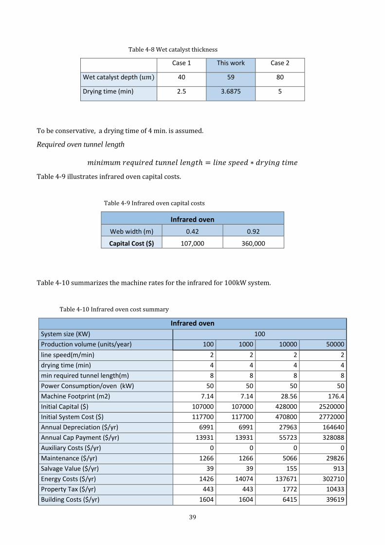
39
Table 4-8 Wet catalyst thickness
Case 1 This work Case 2
Wet catalyst depth (𝑢𝑚) 40 59 80
Drying time (min) 2.5 3.6875 5
To be conservative, a drying time of 4 min. is assumed.
Required oven tunnel length
𝑚𝑖𝑛𝑖𝑚𝑢𝑚 𝑟𝑒𝑞𝑢𝑖𝑟𝑒𝑑 𝑡𝑢𝑛𝑛𝑒𝑙 𝑙𝑒𝑛𝑔𝑡ℎ = 𝑙𝑖𝑛𝑒 𝑠𝑝𝑒𝑒𝑑 ∗ 𝑑𝑟𝑦𝑖𝑛𝑔 𝑡𝑖𝑚𝑒
Table 4-9 illustrates infrared oven capital costs.
Table 4-9 Infrared oven capital costs
Infrared oven
Web width (m) 0.42 0.92
Capital Cost ($) 107,000 360,000
Table 4-10 summarizes the machine rates for the infrared for 100kW system.
Table 4-10 Infrared oven cost summary
Infrared oven
System size (KW) 100
Production volume (units/year) 100 1000 10000 50000
line speed(m/min) 2 2 2 2
drying time (min) 4 4 4 4
min required tunnel length(m) 8 8 8 8
Power Consumption/oven (kW) 50 50 50 50
Machine Footprint (m2) 7.14 7.14 28.56 176.4
Initial Capital ($) 107000 107000 428000 2520000
Initial System Cost ($) 117700 117700 470800 2772000
Annual Depreciation ($/yr) 6991 6991 27963 164640
Annual Cap Payment ($/yr) 13931 13931 55723 328088
Auxiliary Costs ($/yr) 0 0 0 0
Maintenance ($/yr) 1266 1266 5066 29826
Salvage Value ($/yr) 39 39 155 913
Energy Costs ($/yr) 1426 14074 137671 302710
Property Tax ($/yr) 443 443 1772 10433
Building Costs ($/yr) 1604 1604 6415 39619
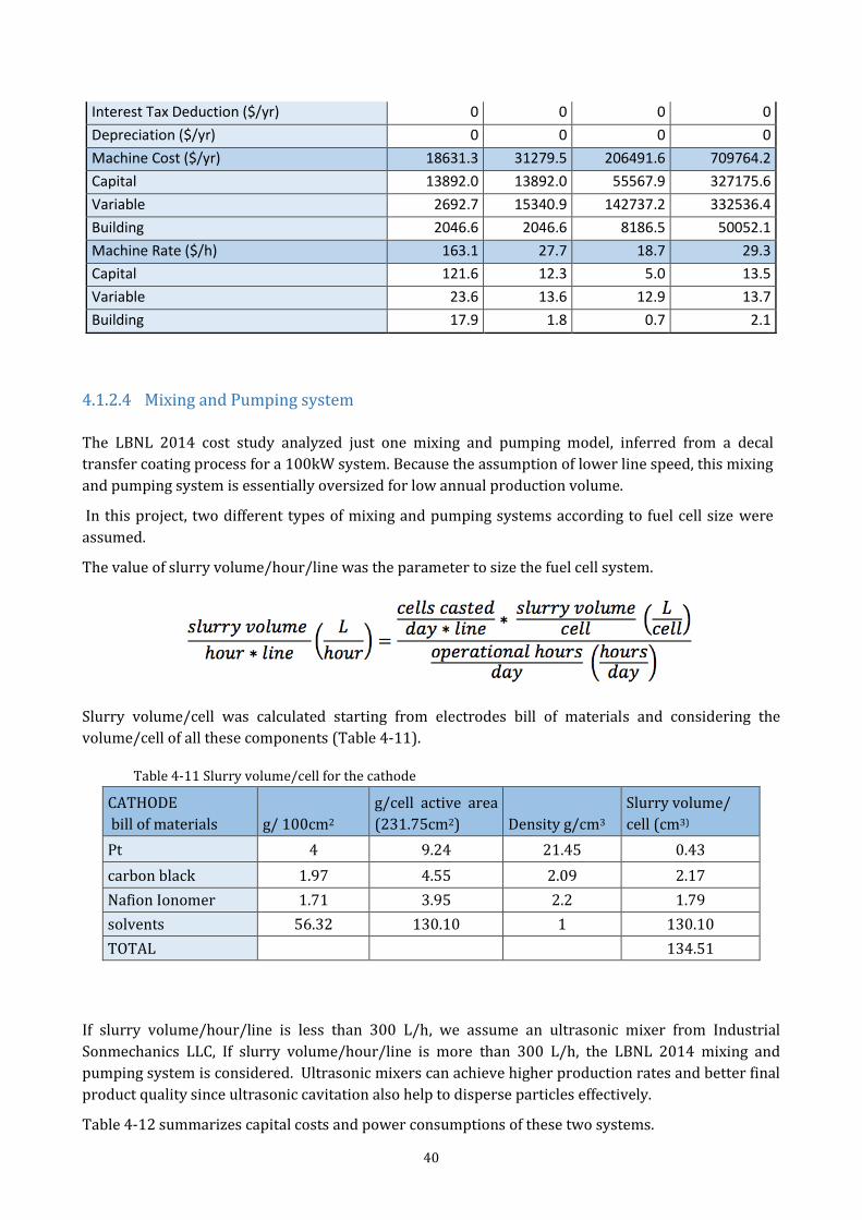
40
Interest Tax Deduction ($/yr) 0 0 0 0
Depreciation ($/yr) 0 0 0 0
Machine Cost ($/yr) 18631.3 31279.5 206491.6 709764.2
Capital 13892.0 13892.0 55567.9 327175.6
Variable 2692.7 15340.9 142737.2 332536.4
Building 2046.6 2046.6 8186.5 50052.1
Machine Rate ($/h) 163.1 27.7 18.7 29.3
Capital 121.6 12.3 5.0 13.5
Variable 23.6 13.6 12.9 13.7
Building 17.9 1.8 0.7 2.1
4.1.2.4 Mixing and Pumping system
The LBNL 2014 cost study analyzed just one mixing and pumping model, inferred from a decal
transfer coating process for a 100kW system. Because the assumption of lower line speed, this mixing
and pumping system is essentially oversized for low annual production volume.
In this project, two different types of mixing and pumping systems according to fuel cell size were
assumed.
The value of slurry volume/hour/line was the parameter to size the fuel cell system.
Slurry volume/cell was calculated starting from electrodes bill of materials and considering the
volume/cell of all these components (Table 4-11).
Table 4-11 Slurry volume/cell for the cathode
CATHODE
bill of materials g/ 100cm2
g/cell active area
(231.75cm2) Density g/cm3
Slurry volume/
cell (cm3)
Pt 4 9.24 21.45 0.43
carbon black 1.97 4.55 2.09 2.17
Nafion Ionomer 1.71 3.95 2.2 1.79
solvents 56.32 130.10 1 130.10
TOTAL
134.51
If slurry volume/hour/line is less than 300 L/h, we assume an ultrasonic mixer from Industrial
Sonmechanics LLC, If slurry volume/hour/line is more than 300 L/h, the LBNL 2014 mixing and
pumping system is considered. Ultrasonic mixers can achieve higher production rates and better final
product quality since ultrasonic cavitation also help to disperse particles effectively.
Table 4-12 summarizes capital costs and power consumptions of these two systems.
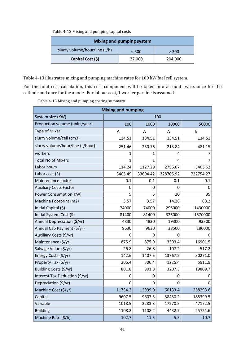
41
Table 4-12 Mixing and pumping capital costs
Mixing and pumping system
slurry volume/hour/line (L/h) < 300 > 300
Capital Cost ($) 37,000 204,000
Table 4-13 illustrates mixing and pumping machine rates for 100 kW fuel cell system.
For the total cost calculation, this cost component will be taken into account twice, once for the
cathode and once for the anode. For labour cost, 1 worker per line is assumed.
Table 4-13 Mixing and pumping costing summary
Mixing and pumping
System size (KW) 100
Production volume (units/year) 100 1000 10000 50000
Type of Mixer A A A B
slurry volume/cell (cm3) 134.51 134.51 134.51 134.51
slurry volume/hour/line (L/hour) 251.46 230.76 213.84 481.15
workers 1 1 4 7
Total No of Mixers 1 1 4 7
Labor hours 114.24 1127.29 2756.67 3463.62
Labor cost ($) 3405.49 33604.42 328705.92 722754.27
Maintenance factor 0.1 0.1 0.1 0.1
Auxiliary Costs Factor 0 0 0 0
Power Consumption(KW) 5 5 20 35
Machine Footprint (m2) 3.57 3.57 14.28 88.2
Initial Capital ($) 74000 74000 296000 1430000
Initial System Cost ($) 81400 81400 326000 1570000
Annual Depreciation ($/yr) 4830 4830 19300 93300
Annual Cap Payment ($/yr) 9630 9630 38500 186000
Auxiliary Costs ($/yr) 0 0 0 0
Maintenance ($/yr) 875.9 875.9 3503.4 16901.5
Salvage Value ($/yr) 26.8 26.8 107.2 517.2
Energy Costs ($/yr) 142.6 1407.5 13767.2 30271.0
Property Tax ($/yr) 306.4 306.4 1225.4 5911.9
Building Costs ($/yr) 801.8 801.8 3207.3 19809.7
Interest Tax Deduction ($/yr) 0 0 0 0
Depreciation ($/yr) 0 0 0 0
Machine Cost ($/yr) 11734.2 12999.0 60133.4 258293.6
Capital 9607.5 9607.5 38430.2 185399.5
Variable 1018.5 2283.3 17270.5 47172.5
Building 1108.2 1108.2 4432.7 25721.6
Machine Rate ($/h) 102.7 11.5 5.5 10.7
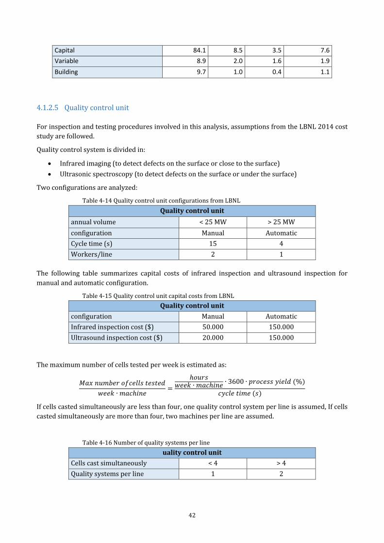
42
Capital 84.1 8.5 3.5 7.6
Variable 8.9 2.0 1.6 1.9
Building 9.7 1.0 0.4 1.1
4.1.2.5 Quality control unit
For inspection and testing procedures involved in this analysis, assumptions from the LBNL 2014 cost
study are followed.
Quality control system is divided in:
Infrared imaging (to detect defects on the surface or close to the surface)
Ultrasonic spectroscopy (to detect defects on the surface or under the surface)
Two configurations are analyzed:
Table 4-14 Quality control unit configurations from LBNL
Quality control unit
annual volume < 25 MW > 25 MW
configuration Manual Automatic
Cycle time (s) 15 4
Workers/line 2 1
The following table summarizes capital costs of infrared inspection and ultrasound inspection for
manual and automatic configuration.
Table 4-15 Quality control unit capital costs from LBNL
Quality control unit
configuration Manual Automatic
Infrared inspection cost ($) 50.000 150.000
Ultrasound inspection cost ($) 20.000 150.000
The maximum number of cells tested per week is estimated as:
𝑀𝑎𝑥 𝑛𝑢𝑚𝑏𝑒𝑟 𝑜𝑓𝑐𝑒𝑙𝑙𝑠 𝑡𝑒𝑠𝑡𝑒𝑑
𝑤𝑒𝑒𝑘 ∙ 𝑚𝑎𝑐ℎ𝑖𝑛𝑒=
ℎ𝑜𝑢𝑟𝑠𝑤𝑒𝑒𝑘 ∙ 𝑚𝑎𝑐ℎ𝑖𝑛𝑒
∙ 3600 ∙ 𝑝𝑟𝑜𝑐𝑒𝑠𝑠 𝑦𝑖𝑒𝑙𝑑 (%)
𝑐𝑦𝑐𝑙𝑒 𝑡𝑖𝑚𝑒 (𝑠)
If cells casted simultaneously are less than four, one quality control system per line is assumed, If cells
casted simultaneously are more than four, two machines per line are assumed.
Table 4-16 Number of quality systems per line
uality control unit
Cells cast simultaneously < 4 > 4
Quality systems per line 1 2
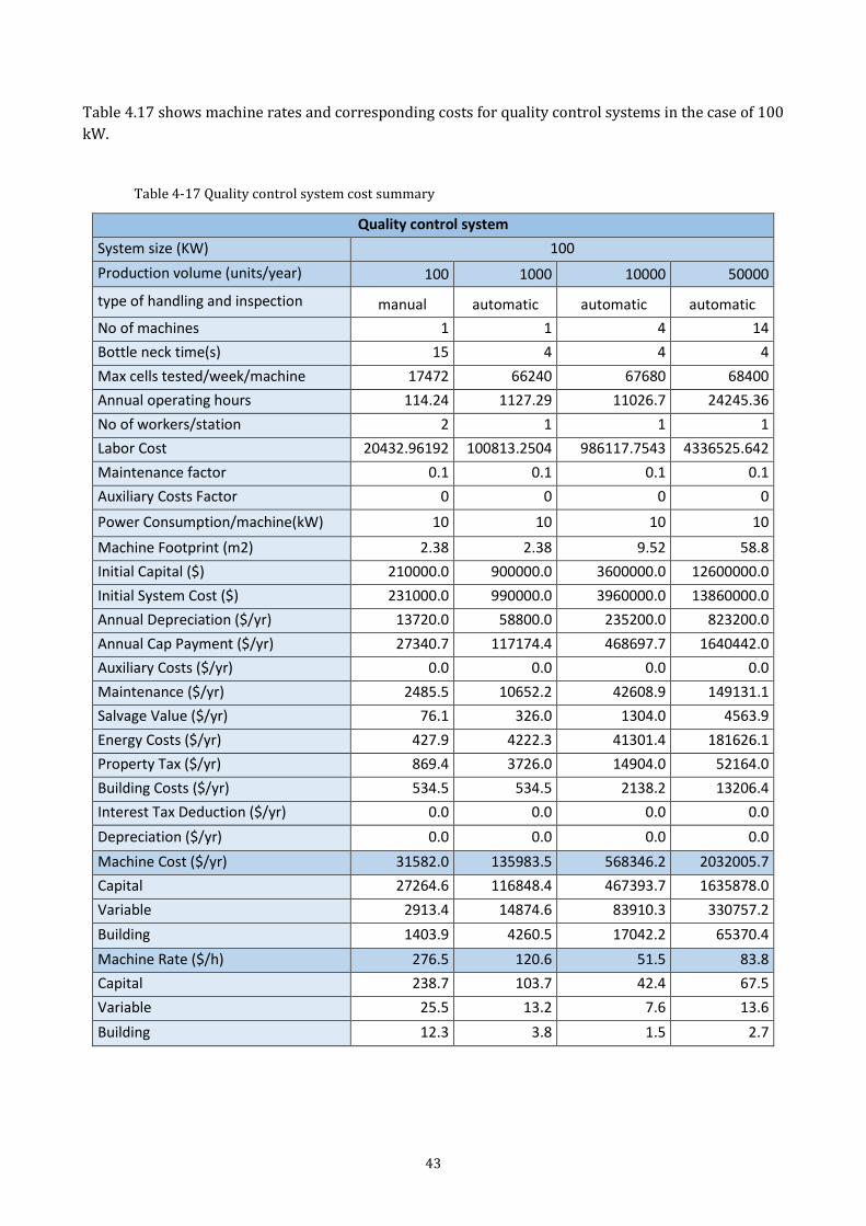
43
Table 4.17 shows machine rates and corresponding costs for quality control systems in the case of 100
kW.
Table 4-17 Quality control system cost summary
Quality control system
System size (KW) 100
Production volume (units/year) 100 1000 10000 50000
type of handling and inspection manual automatic automatic automatic
No of machines 1 1 4 14
Bottle neck time(s) 15 4 4 4
Max cells tested/week/machine 17472 66240 67680 68400
Annual operating hours 114.24 1127.29 11026.7 24245.36
No of workers/station 2 1 1 1
Labor Cost 20432.96192 100813.2504 986117.7543 4336525.642
Maintenance factor 0.1 0.1 0.1 0.1
Auxiliary Costs Factor 0 0 0 0
Power Consumption/machine(kW) 10 10 10 10
Machine Footprint (m2) 2.38 2.38 9.52 58.8
Initial Capital ($) 210000.0 900000.0 3600000.0 12600000.0
Initial System Cost ($) 231000.0 990000.0 3960000.0 13860000.0
Annual Depreciation ($/yr) 13720.0 58800.0 235200.0 823200.0
Annual Cap Payment ($/yr) 27340.7 117174.4 468697.7 1640442.0
Auxiliary Costs ($/yr) 0.0 0.0 0.0 0.0
Maintenance ($/yr) 2485.5 10652.2 42608.9 149131.1
Salvage Value ($/yr) 76.1 326.0 1304.0 4563.9
Energy Costs ($/yr) 427.9 4222.3 41301.4 181626.1
Property Tax ($/yr) 869.4 3726.0 14904.0 52164.0
Building Costs ($/yr) 534.5 534.5 2138.2 13206.4
Interest Tax Deduction ($/yr) 0.0 0.0 0.0 0.0
Depreciation ($/yr) 0.0 0.0 0.0 0.0
Machine Cost ($/yr) 31582.0 135983.5 568346.2 2032005.7
Capital 27264.6 116848.4 467393.7 1635878.0
Variable 2913.4 14874.6 83910.3 330757.2
Building 1403.9 4260.5 17042.2 65370.4
Machine Rate ($/h) 276.5 120.6 51.5 83.8
Capital 238.7 103.7 42.4 67.5
Variable 25.5 13.2 7.6 13.6
Building 12.3 3.8 1.5 2.7
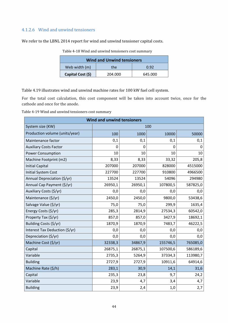
44
4.1.2.6 Wind and unwind tensioners
We refer to the LBNL 2014 report for wind and unwind tensioner capital costs.
Table 4-18 Wind and unwind tensioners cost summary
Wind and Unwind tensioners
Web width (m) the 0.92
Capital Cost ($) 204.000 645.000
Table 4.19 illustrates wind and unwind machine rates for 100 kW fuel cell system.
For the total cost calculation, this cost component will be taken into account twice, once for the
cathode and once for the anode.
Table 4-19 Wind and unwind tensioners cost summary
Wind and unwind tensioners
System size (KW) 100
Production volume (units/year) 100 1000 10000 50000
Maintenance factor 0,1 0,1 0,1 0,1
Auxiliary Costs Factor 0 0 0 0
Power Consumption 10 10 10 10
Machine Footprint (m2) 8,33 8,33 33,32 205,8
Initial Capital 207000 207000 828000 4515000
Initial System Cost 227700 227700 910800 4966500
Annual Depreciation ($/yr) 13524 13524 54096 294980
Annual Cap Payment ($/yr) 26950,1 26950,1 107800,5 587825,0
Auxiliary Costs ($/yr) 0,0 0,0 0,0 0,0
Maintenance ($/yr) 2450,0 2450,0 9800,0 53438,6
Salvage Value ($/yr) 75,0 75,0 299,9 1635,4
Energy Costs ($/yr) 285,3 2814,9 27534,3 60542,0
Property Tax ($/yr) 857,0 857,0 3427,9 18692,1
Building Costs ($/yr) 1870,9 1870,9 7483,7 46222,5
Interest Tax Deduction ($/yr) 0,0 0,0 0,0 0,0
Depreciation ($/yr) 0,0 0,0 0,0 0,0
Machine Cost ($/yr) 32338,3 34867,9 155746,5 765085,0
Capital 26875,1 26875,1 107500,6 586189,6
Variable 2735,3 5264,9 37334,3 113980,7
Building 2727,9 2727,9 10911,6 64914,6
Machine Rate ($/h) 283,1 30,9 14,1 31,6
Capital 235,3 23,8 9,7 24,2
Variable 23,9 4,7 3,4 4,7
Building 23,9 2,4 1,0 2,7
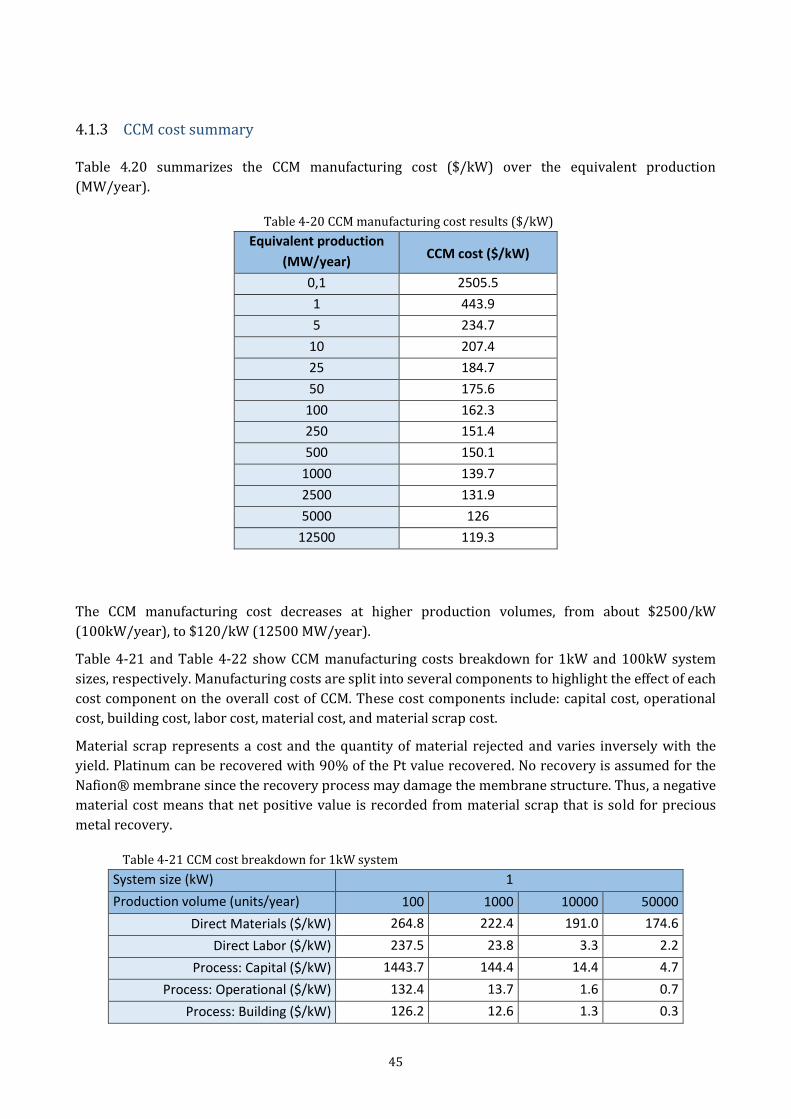
45
4.1.3 CCM cost summary Table 4.20 summarizes the CCM manufacturing cost ($/kW) over the equivalent production
(MW/year).
Table 4-20 CCM manufacturing cost results ($/kW)
Equivalent production
(MW/year) CCM cost ($/kW)
0,1 2505.5
1 443.9
5 234.7
10 207.4
25 184.7
50 175.6
100 162.3
250 151.4
500 150.1
1000 139.7
2500 131.9
5000 126
12500 119.3
The CCM manufacturing cost decreases at higher production volumes, from about $2500/kW
(100kW/year), to $120/kW (12500 MW/year).
Table 4-21 and Table 4-22 show CCM manufacturing costs breakdown for 1kW and 100kW system
sizes, respectively. Manufacturing costs are split into several components to highlight the effect of each
cost component on the overall cost of CCM. These cost components include: capital cost, operational
cost, building cost, labor cost, material cost, and material scrap cost.
Material scrap represents a cost and the quantity of material rejected and varies inversely with the
yield. Platinum can be recovered with 90% of the Pt value recovered. No recovery is assumed for the
Nafion® membrane since the recovery process may damage the membrane structure. Thus, a negative
material cost means that net positive value is recorded from material scrap that is sold for precious
metal recovery.
Table 4-21 CCM cost breakdown for 1kW system
System size (kW) 1
Production volume (units/year) 100 1000 10000 50000
Direct Materials ($/kW) 264.8 222.4 191.0 174.6
Direct Labor ($/kW) 237.5 23.8 3.3 2.2
Process: Capital ($/kW) 1443.7 144.4 14.4 4.7
Process: Operational ($/kW) 132.4 13.7 1.6 0.7
Process: Building ($/kW) 126.2 12.6 1.3 0.3
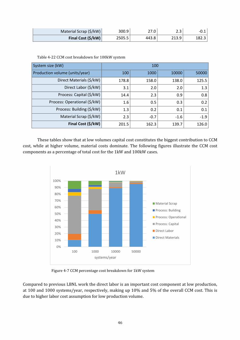
46
Material Scrap ($/kW) 300.9 27.0 2.3 -0.1
Final Cost ($/kW) 2505.5 443.8 213.9 182.3
Table 4-22 CCM cost breakdown for 100kW system
System size (kW) 100
Production volume (units/year) 100 1000 10000 50000
Direct Materials ($/kW) 178.8 158.0 138.0 125.5
Direct Labor ($/kW) 3.1 2.0 2.0 1.3
Process: Capital ($/kW) 14.4 2.3 0.9 0.8
Process: Operational ($/kW) 1.6 0.5 0.3 0.2
Process: Building ($/kW) 1.3 0.2 0.1 0.1
Material Scrap ($/kW) 2.3 -0.7 -1.6 -1.9
Final Cost ($/kW) 201.5 162.3 139.7 126.0
These tables show that at low volumes capital cost constitutes the biggest contribution to CCM
cost, while at higher volume, material costs dominate. The following figures illustrate the CCM cost
components as a percentage of total cost for the 1kW and 100kW cases.
Figure 4-7 CCM percentage cost breakdown for 1kW system
Compared to previous LBNL work the direct labor is an important cost component at low production,
at 100 and 1000 systems/year, respectively, making up 10% and 5% of the overall CCM cost. This is
due to higher labor cost assumption for low production volume.
0%
10%
20%
30%
40%
50%
60%
70%
80%
90%
100%
100 1000 10000 50000
systems/year
1kW
Material Scrap
Process: Building
Process: Operational
Process: Capital
Direct Labor
Direct Materials
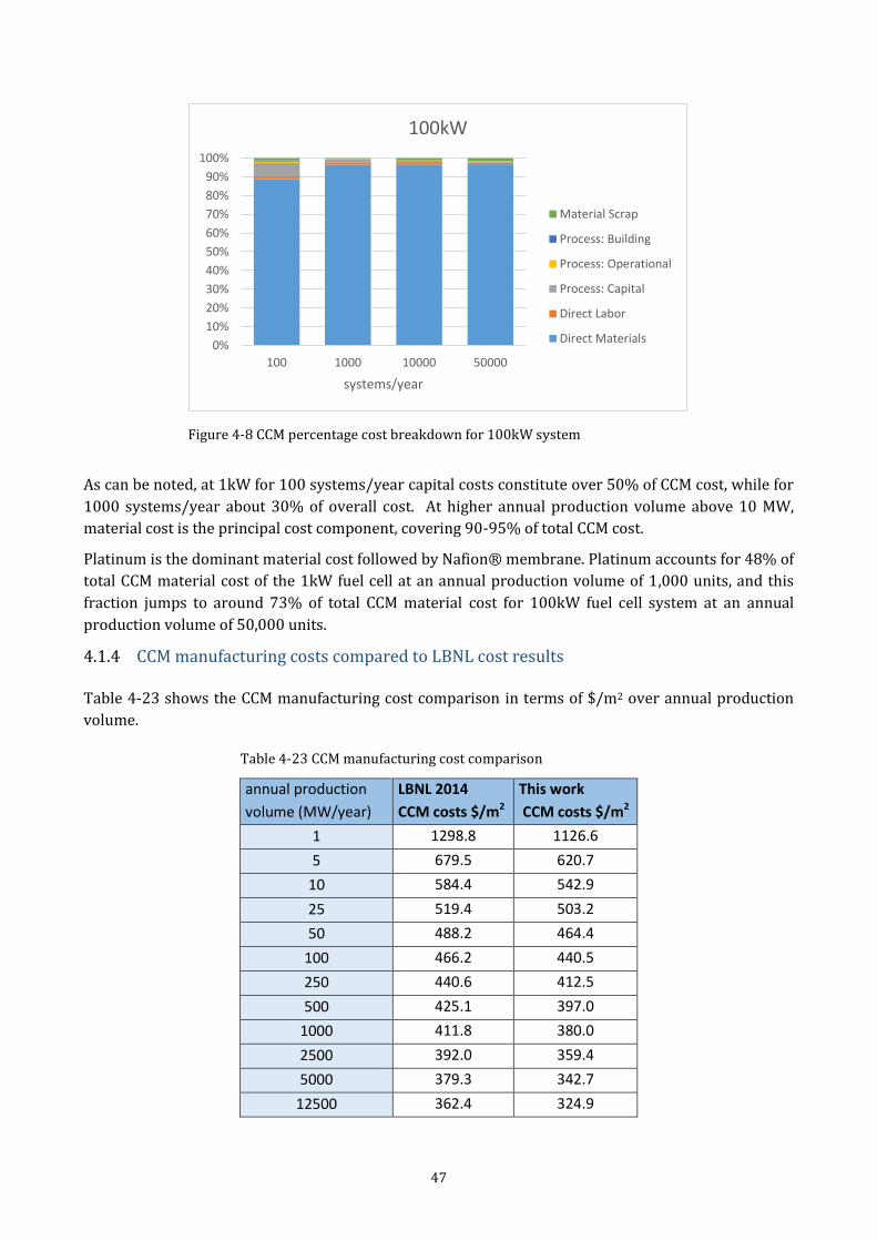
47
Figure 4-8 CCM percentage cost breakdown for 100kW system
As can be noted, at 1kW for 100 systems/year capital costs constitute over 50% of CCM cost, while for
1000 systems/year about 30% of overall cost. At higher annual production volume above 10 MW,
material cost is the principal cost component, covering 90-95% of total CCM cost.
Platinum is the dominant material cost followed by Nafion® membrane. Platinum accounts for 48% of
total CCM material cost of the 1kW fuel cell at an annual production volume of 1,000 units, and this
fraction jumps to around 73% of total CCM material cost for 100kW fuel cell system at an annual
production volume of 50,000 units.
4.1.4 CCM manufacturing costs compared to LBNL cost results Table 4-23 shows the CCM manufacturing cost comparison in terms of $/m2 over annual production
volume.
Table 4-23 CCM manufacturing cost comparison
annual production
volume (MW/year)
LBNL 2014
CCM costs $/m2
This work
CCM costs $/m2
1 1298.8 1126.6
5 679.5 620.7
10 584.4 542.9
25 519.4 503.2
50 488.2 464.4
100 466.2 440.5
250 440.6 412.5
500 425.1 397.0
1000 411.8 380.0
2500 392.0 359.4
5000 379.3 342.7
12500 362.4 324.9
0%
10%
20%
30%
40%
50%
60%
70%
80%
90%
100%
100 1000 10000 50000
systems/year
100kW
Material Scrap
Process: Building
Process: Operational
Process: Capital
Direct Labor
Direct Materials
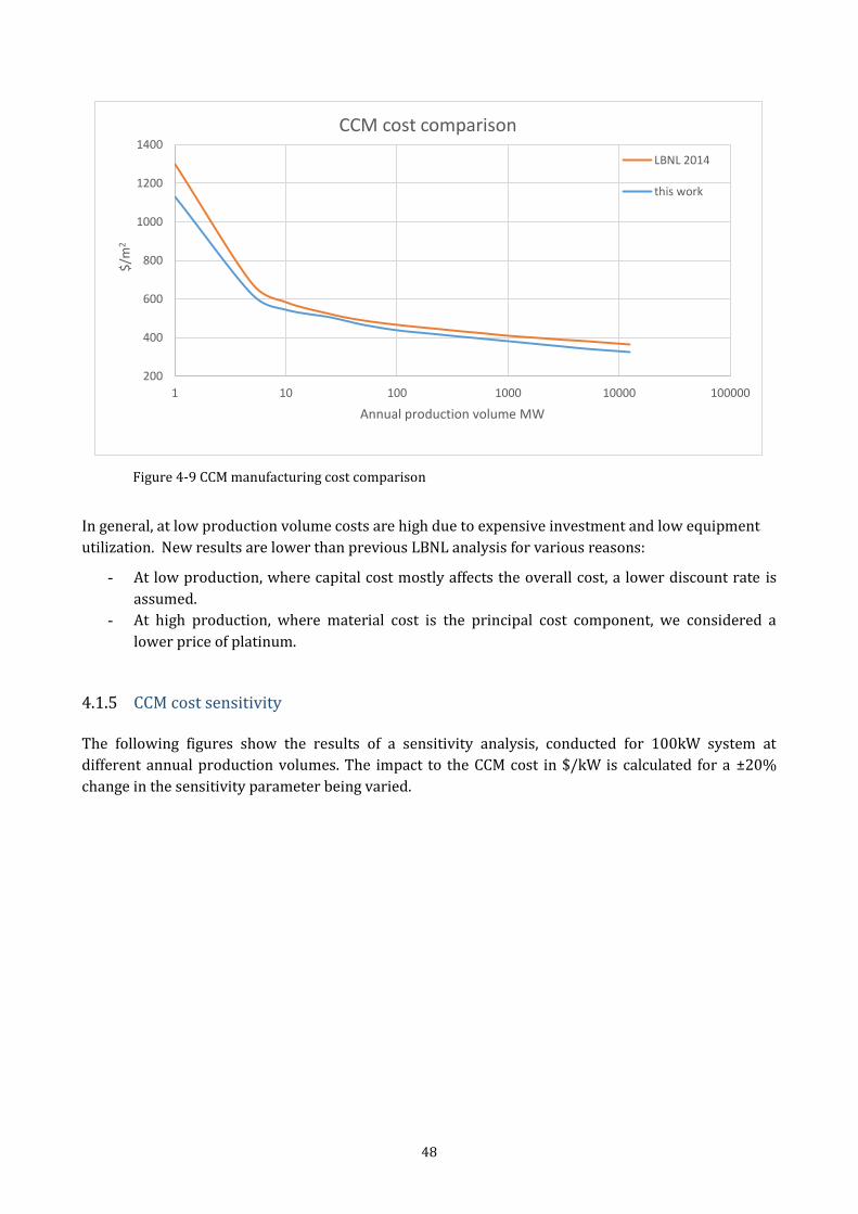
48
Figure 4-9 CCM manufacturing cost comparison
In general, at low production volume costs are high due to expensive investment and low equipment
utilization. New results are lower than previous LBNL analysis for various reasons:
- At low production, where capital cost mostly affects the overall cost, a lower discount rate is
assumed.
- At high production, where material cost is the principal cost component, we considered a
lower price of platinum.
4.1.5 CCM cost sensitivity The following figures show the results of a sensitivity analysis, conducted for 100kW system at
different annual production volumes. The impact to the CCM cost in $/kW is calculated for a ±20%
change in the sensitivity parameter being varied.
200
400
600
800
1000
1200
1400
1 10 100 1000 10000 100000
$/m
2
Annual production volume MW
CCM cost comparison
LBNL 2014
this work
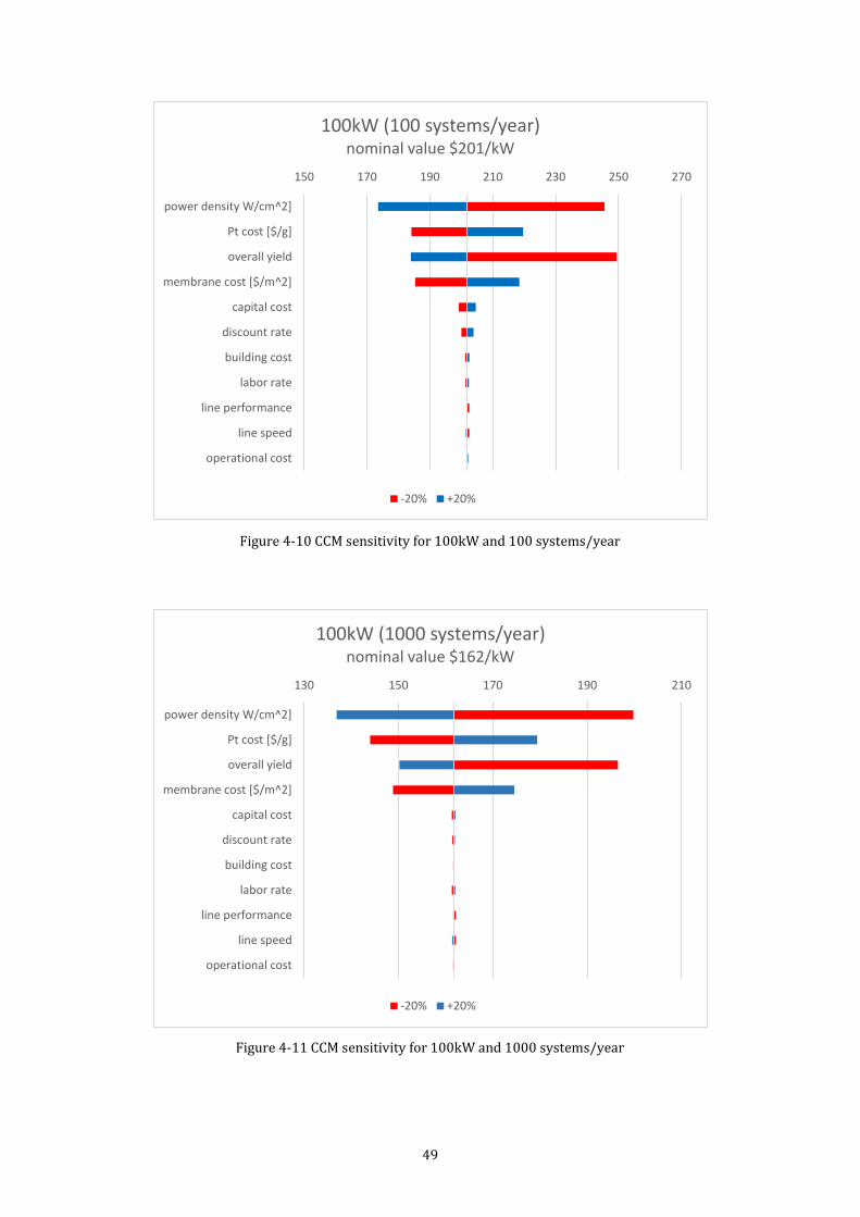
49
Figure 4-10 CCM sensitivity for 100kW and 100 systems/year
Figure 4-11 CCM sensitivity for 100kW and 1000 systems/year
150 170 190 210 230 250 270
power density W/cm^2]
Pt cost [$/g]
overall yield
membrane cost [$/m^2]
capital cost
discount rate
building cost
labor rate
line performance
line speed
operational cost
100kW (100 systems/year) nominal value $201/kW
-20% +20%
130 150 170 190 210
power density W/cm^2]
Pt cost [$/g]
overall yield
membrane cost [$/m^2]
capital cost
discount rate
building cost
labor rate
line performance
line speed
operational cost
100kW (1000 systems/year) nominal value $162/kW
-20% +20%
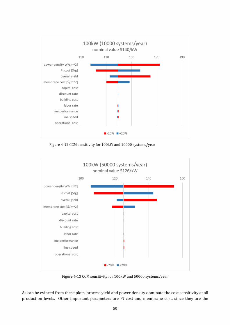
50
Figure 4-12 CCM sensitivity for 100kW and 10000 systems/year
Figure 4-13 CCM sensitivity for 100kW and 50000 systems/year
As can be evinced from these plots, process yield and power density dominate the cost sensitivity at all
production levels. Other important parameters are Pt cost and membrane cost, since they are the
110 130 150 170 190
power density W/cm^2]
Pt cost [$/g]
overall yield
membrane cost [$/m^2]
capital cost
discount rate
building cost
labor rate
line performance
line speed
operational cost
100kW (10000 systems/year) nominal value $140/kW
-20% +20%
100 120 140 160
power density W/cm^2]
Pt cost [$/g]
overall yield
membrane cost [$/m^2]
capital cost
discount rate
building cost
labor rate
line performance
line speed
operational cost
100kW (50000 systems/year) nominal value $126/kW
-20% +20%
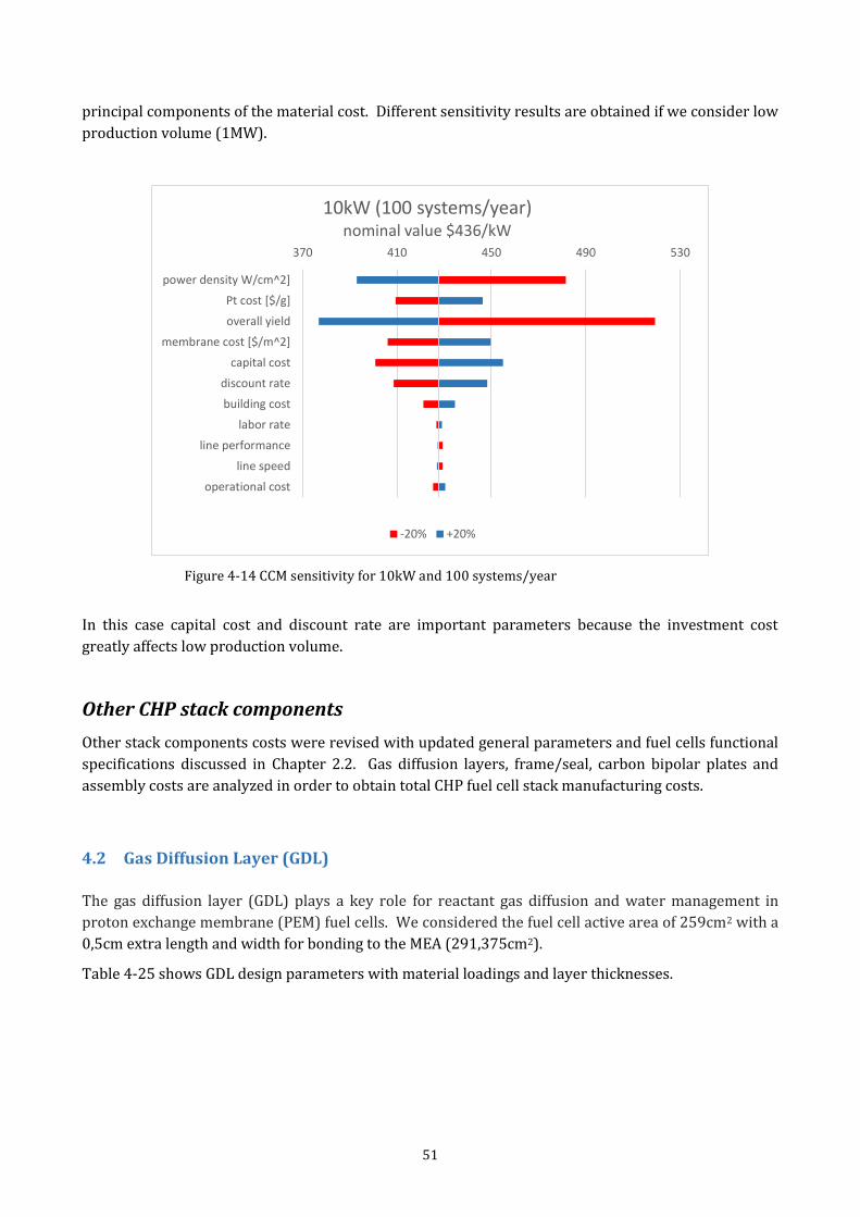
51
principal components of the material cost. Different sensitivity results are obtained if we consider low
production volume (1MW).
Figure 4-14 CCM sensitivity for 10kW and 100 systems/year
In this case capital cost and discount rate are important parameters because the investment cost
greatly affects low production volume.
Other CHP stack components
Other stack components costs were revised with updated general parameters and fuel cells functional
specifications discussed in Chapter 2.2. Gas diffusion layers, frame/seal, carbon bipolar plates and
assembly costs are analyzed in order to obtain total CHP fuel cell stack manufacturing costs.
4.2 Gas Diffusion Layer (GDL)
The gas diffusion layer (GDL) plays a key role for reactant gas diffusion and water management in
proton exchange membrane (PEM) fuel cells. We considered the fuel cell active area of 259cm2 with a
0,5cm extra length and width for bonding to the MEA (291,375cm2).
Table 4-25 shows GDL design parameters with material loadings and layer thicknesses.
370 410 450 490 530
power density W/cm^2]
Pt cost [$/g]
overall yield
membrane cost [$/m^2]
capital cost
discount rate
building cost
labor rate
line performance
line speed
operational cost
10kW (100 systems/year) nominal value $436/kW
-20% +20%
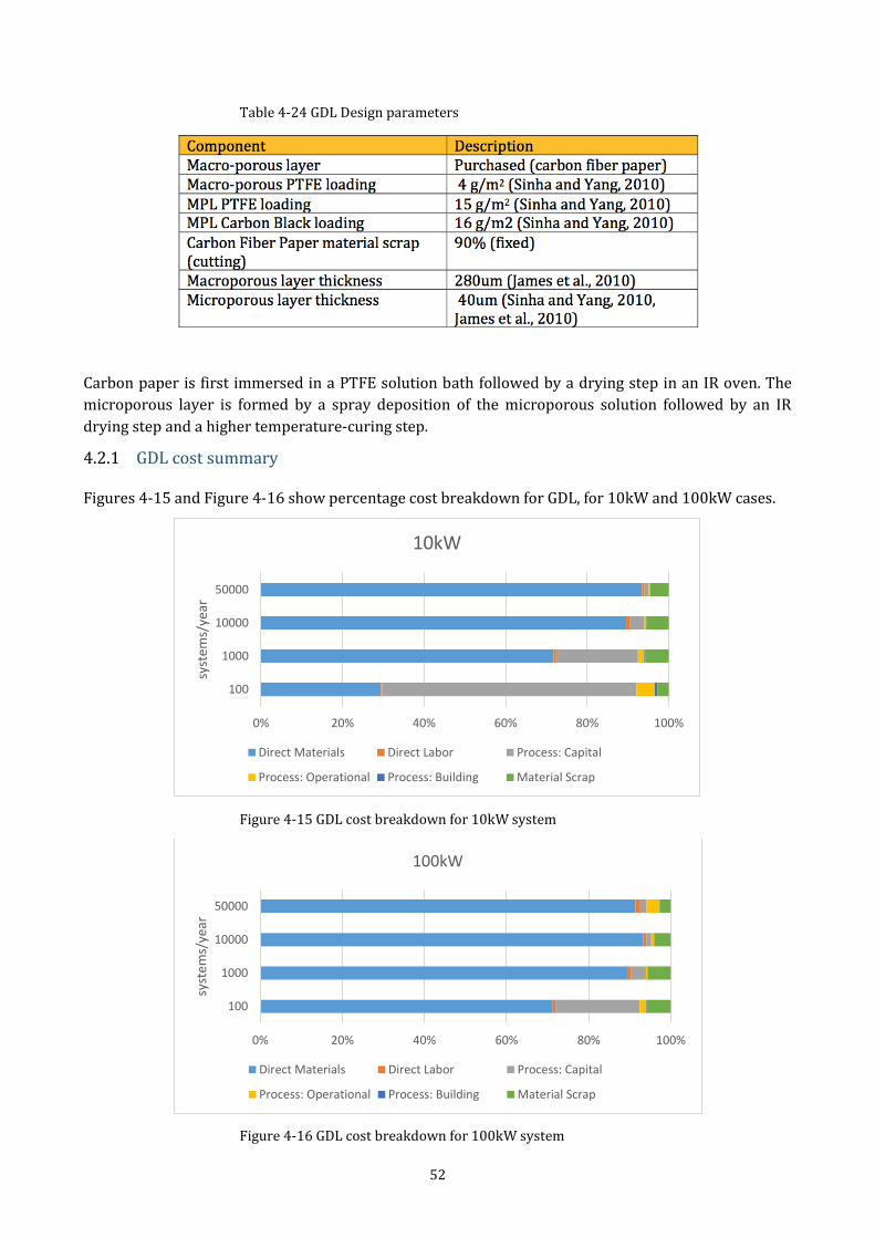
52
Table 4-24 GDL Design parameters
Carbon paper is first immersed in a PTFE solution bath followed by a drying step in an IR oven. The
microporous layer is formed by a spray deposition of the microporous solution followed by an IR
drying step and a higher temperature-curing step.
4.2.1 GDL cost summary
Figures 4-15 and Figure 4-16 show percentage cost breakdown for GDL, for 10kW and 100kW cases.
Figure 4-15 GDL cost breakdown for 10kW system
Figure 4-16 GDL cost breakdown for 100kW system
0% 20% 40% 60% 80% 100%
100
1000
10000
50000
syst
ems/
year
10kW
Direct Materials Direct Labor Process: Capital
Process: Operational Process: Building Material Scrap
0% 20% 40% 60% 80% 100%
100
1000
10000
50000
syst
ems/
year
100kW
Direct Materials Direct Labor Process: Capital
Process: Operational Process: Building Material Scrap
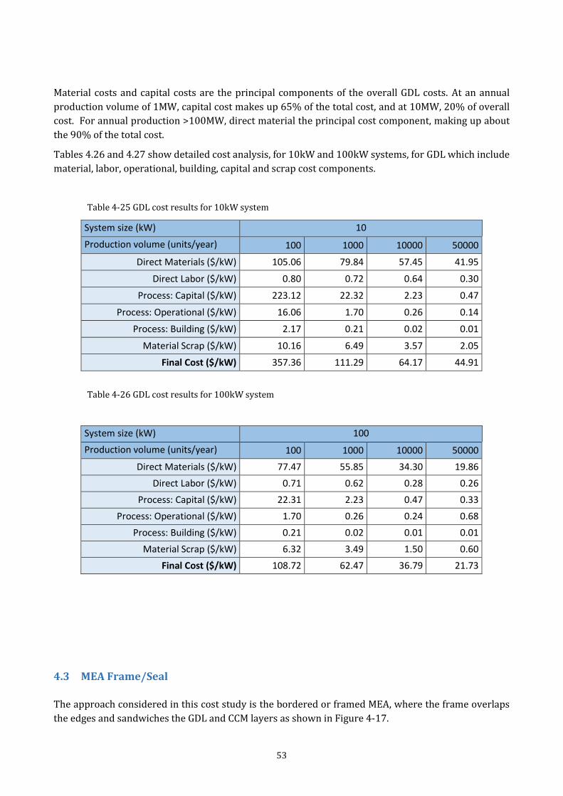
53
Material costs and capital costs are the principal components of the overall GDL costs. At an annual
production volume of 1MW, capital cost makes up 65% of the total cost, and at 10MW, 20% of overall
cost. For annual production >100MW, direct material the principal cost component, making up about
the 90% of the total cost.
Tables 4.26 and 4.27 show detailed cost analysis, for 10kW and 100kW systems, for GDL which include
material, labor, operational, building, capital and scrap cost components.
Table 4-25 GDL cost results for 10kW system
System size (kW) 10
Production volume (units/year) 100 1000 10000 50000
Direct Materials ($/kW) 105.06 79.84 57.45 41.95
Direct Labor ($/kW) 0.80 0.72 0.64 0.30
Process: Capital ($/kW) 223.12 22.32 2.23 0.47
Process: Operational ($/kW) 16.06 1.70 0.26 0.14
Process: Building ($/kW) 2.17 0.21 0.02 0.01
Material Scrap ($/kW) 10.16 6.49 3.57 2.05
Final Cost ($/kW) 357.36 111.29 64.17 44.91
Table 4-26 GDL cost results for 100kW system
System size (kW) 100
Production volume (units/year) 100 1000 10000 50000
Direct Materials ($/kW) 77.47 55.85 34.30 19.86
Direct Labor ($/kW) 0.71 0.62 0.28 0.26
Process: Capital ($/kW) 22.31 2.23 0.47 0.33
Process: Operational ($/kW) 1.70 0.26 0.24 0.68
Process: Building ($/kW) 0.21 0.02 0.01 0.01
Material Scrap ($/kW) 6.32 3.49 1.50 0.60
Final Cost ($/kW) 108.72 62.47 36.79 21.73
4.3 MEA Frame/Seal
The approach considered in this cost study is the bordered or framed MEA, where the frame overlaps
the edges and sandwiches the GDL and CCM layers as shown in Figure 4-17.
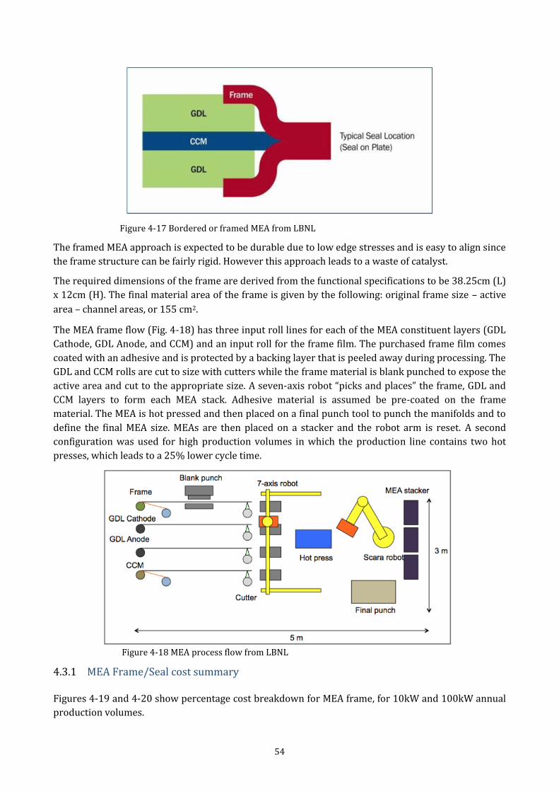
54
Figure 4-17 Bordered or framed MEA from LBNL
The framed MEA approach is expected to be durable due to low edge stresses and is easy to align since
the frame structure can be fairly rigid. However this approach leads to a waste of catalyst.
The required dimensions of the frame are derived from the functional specifications to be 38.25cm (L)
x 12cm (H). The final material area of the frame is given by the following: original frame size – active
area – channel areas, or 155 cm2.
The MEA frame flow (Fig. 4-18) has three input roll lines for each of the MEA constituent layers (GDL
Cathode, GDL Anode, and CCM) and an input roll for the frame film. The purchased frame film comes
coated with an adhesive and is protected by a backing layer that is peeled away during processing. The
GDL and CCM rolls are cut to size with cutters while the frame material is blank punched to expose the
active area and cut to the appropriate size. A seven-axis robot “picks and places” the frame, GDL and
CCM layers to form each MEA stack. Adhesive material is assumed be pre-coated on the frame
material. The MEA is hot pressed and then placed on a final punch tool to punch the manifolds and to
define the final MEA size. MEAs are then placed on a stacker and the robot arm is reset. A second
configuration was used for high production volumes in which the production line contains two hot
presses, which leads to a 25% lower cycle time.
Figure 4-18 MEA process flow from LBNL
4.3.1 MEA Frame/Seal cost summary Figures 4-19 and 4-20 show percentage cost breakdown for MEA frame, for 10kW and 100kW annual
production volumes.
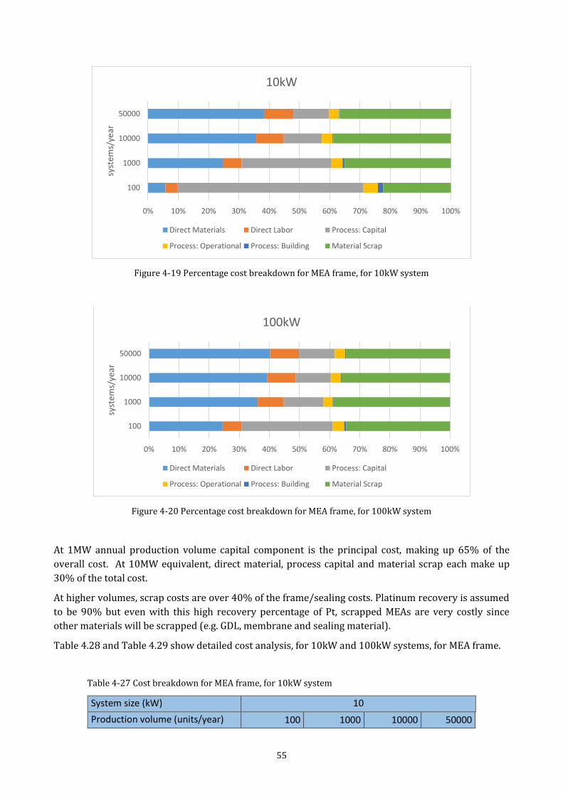
55
Figure 4-19 Percentage cost breakdown for MEA frame, for 10kW system
Figure 4-20 Percentage cost breakdown for MEA frame, for 100kW system
At 1MW annual production volume capital component is the principal cost, making up 65% of the
overall cost. At 10MW equivalent, direct material, process capital and material scrap each make up
30% of the total cost.
At higher volumes, scrap costs are over 40% of the frame/sealing costs. Platinum recovery is assumed
to be 90% but even with this high recovery percentage of Pt, scrapped MEAs are very costly since
other materials will be scrapped (e.g. GDL, membrane and sealing material).
Table 4.28 and Table 4.29 show detailed cost analysis, for 10kW and 100kW systems, for MEA frame.
Table 4-27 Cost breakdown for MEA frame, for 10kW system
System size (kW) 10
Production volume (units/year) 100 1000 10000 50000
0% 10% 20% 30% 40% 50% 60% 70% 80% 90% 100%
100
1000
10000
50000sy
stem
s/ye
ar
10kW
Direct Materials Direct Labor Process: Capital
Process: Operational Process: Building Material Scrap
0% 10% 20% 30% 40% 50% 60% 70% 80% 90% 100%
100
1000
10000
50000
syst
ems/
year
100kW
Direct Materials Direct Labor Process: Capital
Process: Operational Process: Building Material Scrap
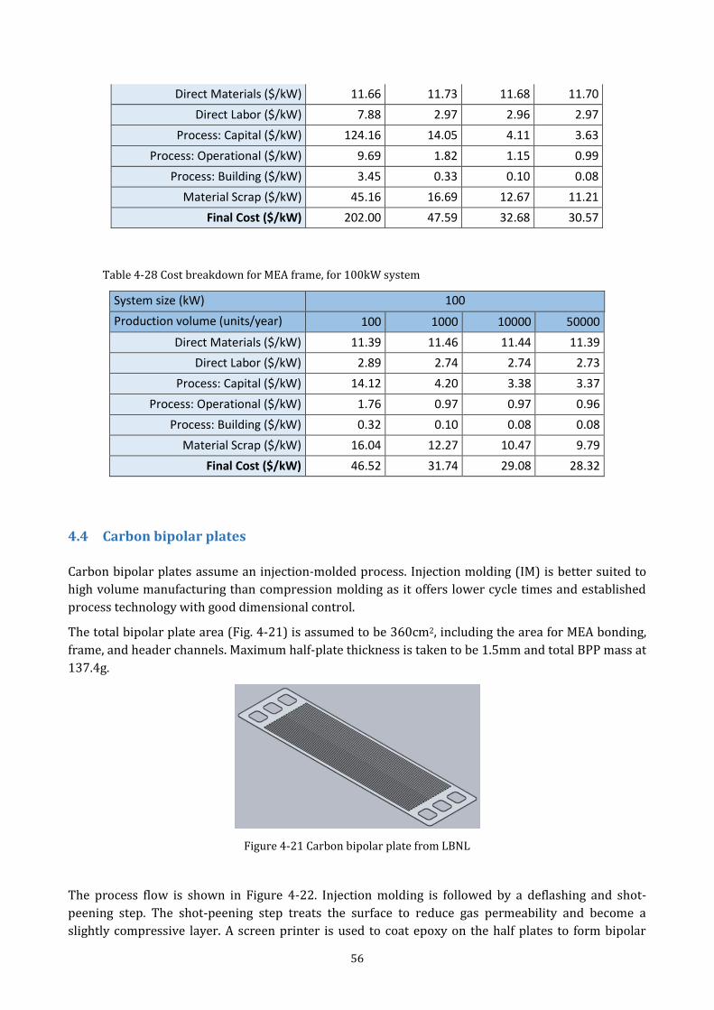
56
Direct Materials ($/kW) 11.66 11.73 11.68 11.70
Direct Labor ($/kW) 7.88 2.97 2.96 2.97
Process: Capital ($/kW) 124.16 14.05 4.11 3.63
Process: Operational ($/kW) 9.69 1.82 1.15 0.99
Process: Building ($/kW) 3.45 0.33 0.10 0.08
Material Scrap ($/kW) 45.16 16.69 12.67 11.21
Final Cost ($/kW) 202.00 47.59 32.68 30.57
Table 4-28 Cost breakdown for MEA frame, for 100kW system
System size (kW) 100
Production volume (units/year) 100 1000 10000 50000
Direct Materials ($/kW) 11.39 11.46 11.44 11.39
Direct Labor ($/kW) 2.89 2.74 2.74 2.73
Process: Capital ($/kW) 14.12 4.20 3.38 3.37
Process: Operational ($/kW) 1.76 0.97 0.97 0.96
Process: Building ($/kW) 0.32 0.10 0.08 0.08
Material Scrap ($/kW) 16.04 12.27 10.47 9.79
Final Cost ($/kW) 46.52 31.74 29.08 28.32
4.4 Carbon bipolar plates
Carbon bipolar plates assume an injection-molded process. Injection molding (IM) is better suited to
high volume manufacturing than compression molding as it offers lower cycle times and established
process technology with good dimensional control.
The total bipolar plate area (Fig. 4-21) is assumed to be 360cm2, including the area for MEA bonding,
frame, and header channels. Maximum half-plate thickness is taken to be 1.5mm and total BPP mass at
137.4g.
Figure 4-21 Carbon bipolar plate from LBNL
The process flow is shown in Figure 4-22. Injection molding is followed by a deflashing and shot-
peening step. The shot-peening step treats the surface to reduce gas permeability and become a
slightly compressive layer. A screen printer is used to coat epoxy on the half plates to form bipolar
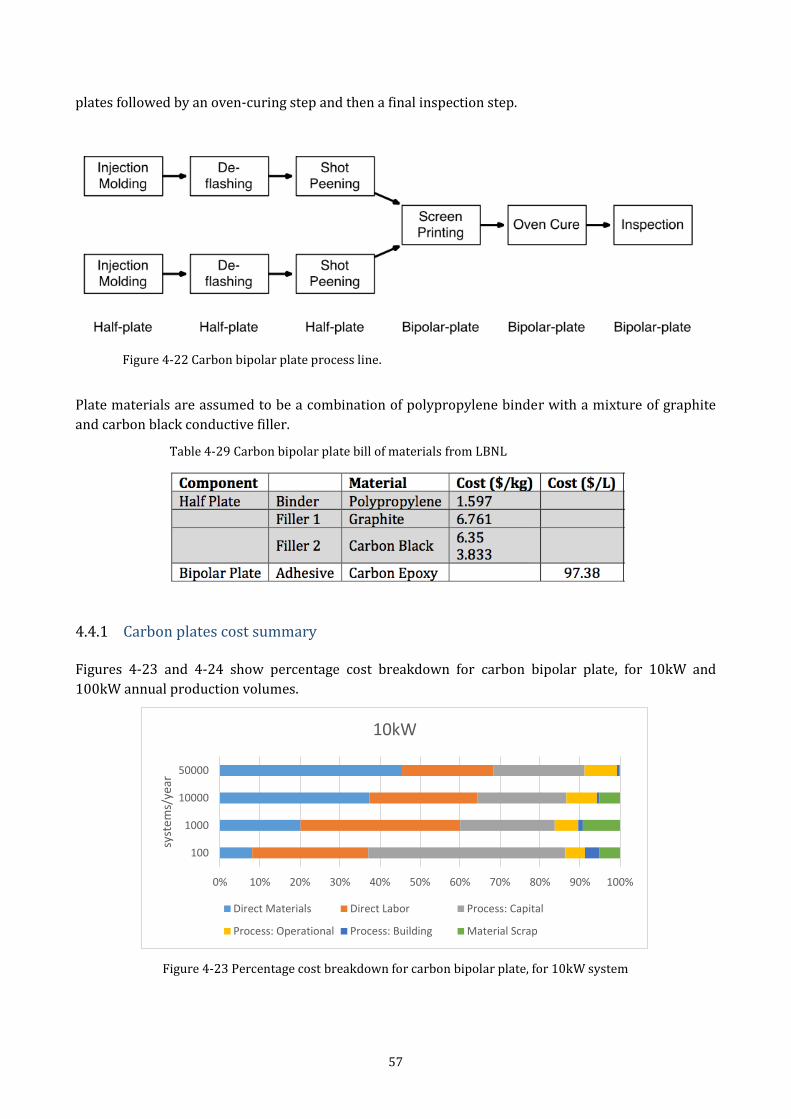
57
plates followed by an oven-curing step and then a final inspection step.
Figure 4-22 Carbon bipolar plate process line.
Plate materials are assumed to be a combination of polypropylene binder with a mixture of graphite
and carbon black conductive filler.
Table 4-29 Carbon bipolar plate bill of materials from LBNL
4.4.1 Carbon plates cost summary Figures 4-23 and 4-24 show percentage cost breakdown for carbon bipolar plate, for 10kW and
100kW annual production volumes.
Figure 4-23 Percentage cost breakdown for carbon bipolar plate, for 10kW system
0% 10% 20% 30% 40% 50% 60% 70% 80% 90% 100%
100
1000
10000
50000
syst
ems/
year
10kW
Direct Materials Direct Labor Process: Capital
Process: Operational Process: Building Material Scrap
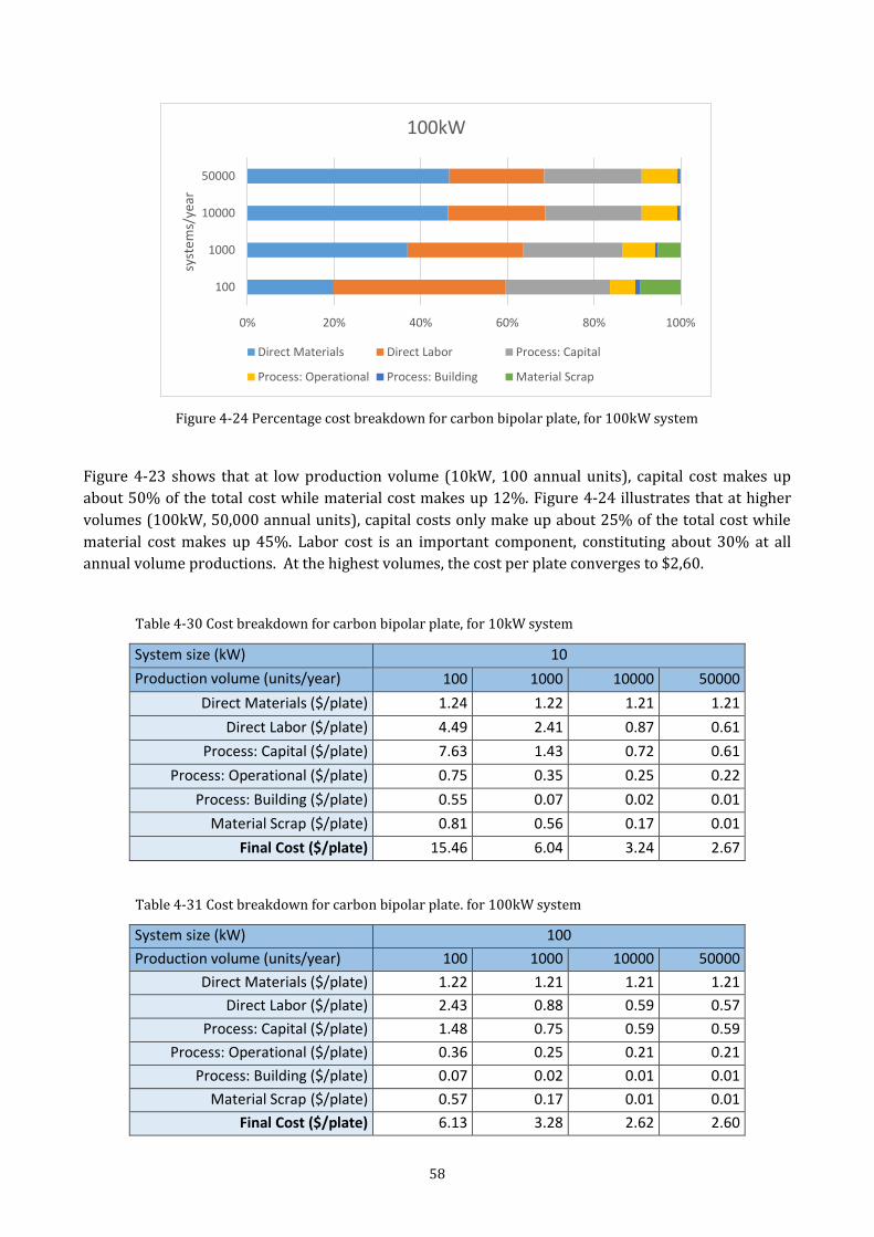
58
Figure 4-24 Percentage cost breakdown for carbon bipolar plate, for 100kW system
Figure 4-23 shows that at low production volume (10kW, 100 annual units), capital cost makes up
about 50% of the total cost while material cost makes up 12%. Figure 4-24 illustrates that at higher
volumes (100kW, 50,000 annual units), capital costs only make up about 25% of the total cost while
material cost makes up 45%. Labor cost is an important component, constituting about 30% at all
annual volume productions. At the highest volumes, the cost per plate converges to $2,60.
Table 4-30 Cost breakdown for carbon bipolar plate, for 10kW system
System size (kW) 10
Production volume (units/year) 100 1000 10000 50000
Direct Materials ($/plate) 1.24 1.22 1.21 1.21
Direct Labor ($/plate) 4.49 2.41 0.87 0.61
Process: Capital ($/plate) 7.63 1.43 0.72 0.61
Process: Operational ($/plate) 0.75 0.35 0.25 0.22
Process: Building ($/plate) 0.55 0.07 0.02 0.01
Material Scrap ($/plate) 0.81 0.56 0.17 0.01
Final Cost ($/plate) 15.46 6.04 3.24 2.67
Table 4-31 Cost breakdown for carbon bipolar plate. for 100kW system
System size (kW) 100
Production volume (units/year) 100 1000 10000 50000
Direct Materials ($/plate) 1.22 1.21 1.21 1.21
Direct Labor ($/plate) 2.43 0.88 0.59 0.57
Process: Capital ($/plate) 1.48 0.75 0.59 0.59
Process: Operational ($/plate) 0.36 0.25 0.21 0.21
Process: Building ($/plate) 0.07 0.02 0.01 0.01
Material Scrap ($/plate) 0.57 0.17 0.01 0.01
Final Cost ($/plate) 6.13 3.28 2.62 2.60
0% 20% 40% 60% 80% 100%
100
1000
10000
50000sy
stem
s/ye
ar
100kW
Direct Materials Direct Labor Process: Capital
Process: Operational Process: Building Material Scrap
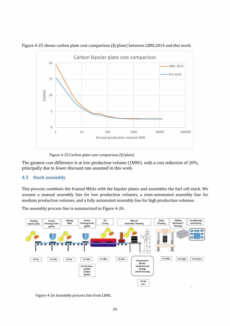
59
Figure 4-25 shows carbon plate cost comparison ($/plate) between LBNL2014 and this work.
Figure 4-25 Carbon plate cost comparison ($/plate)
The greatest cost difference is at low production volume (1MW), with a cost reduction of 20%,
principally due to lower discount rate assumed in this work.
4.5 Stack assembly
This process combines the framed MEAs with the bipolar plates and assembles the fuel cell stack. We
assume a manual assembly line for low production volumes, a semi-automated assembly line for
medium production volumes, and a fully automated assembly line for high production volumes.
The assembly process line is summarized in Figure 4-26.
Figure 4-26 Assembly process line from LBNL
0
5
10
15
20
1 10 100 1000 10000 100000
$/p
late
Annual production volume MW
Carbon bipolar plate cost comparison
LBNL 2014
this work
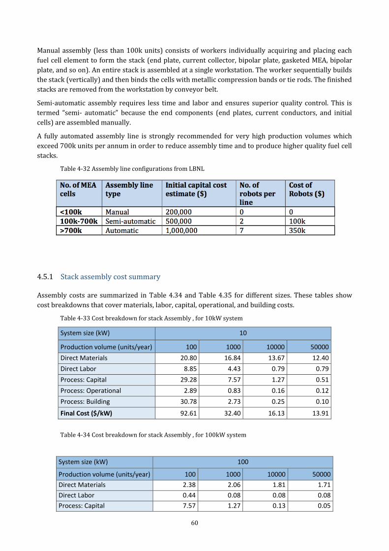
60
Manual assembly (less than 100k units) consists of workers individually acquiring and placing each
fuel cell element to form the stack (end plate, current collector, bipolar plate, gasketed MEA, bipolar
plate, and so on). An entire stack is assembled at a single workstation. The worker sequentially builds
the stack (vertically) and then binds the cells with metallic compression bands or tie rods. The finished
stacks are removed from the workstation by conveyor belt.
Semi‐automatic assembly requires less time and labor and ensures superior quality control. This is
termed “semi‐ automatic” because the end components (end plates, current conductors, and initial
cells) are assembled manually.
A fully automated assembly line is strongly recommended for very high production volumes which
exceed 700k units per annum in order to reduce assembly time and to produce higher quality fuel cell
stacks.
Table 4-32 Assembly line configurations from LBNL
4.5.1 Stack assembly cost summary Assembly costs are summarized in Table 4.34 and Table 4.35 for different sizes. These tables show
cost breakdowns that cover materials, labor, capital, operational, and building costs.
Table 4-33 Cost breakdown for stack Assembly , for 10kW system
System size (kW) 10
Production volume (units/year) 100 1000 10000 50000
Direct Materials 20.80 16.84 13.67 12.40
Direct Labor 8.85 4.43 0.79 0.79
Process: Capital 29.28 7.57 1.27 0.51
Process: Operational 2.89 0.83 0.16 0.12
Process: Building 30.78 2.73 0.25 0.10
Final Cost ($/kW) 92.61 32.40 16.13 13.91
Table 4-34 Cost breakdown for stack Assembly , for 100kW system
System size (kW) 100
Production volume (units/year) 100 1000 10000 50000
Direct Materials 2.38 2.06 1.81 1.71
Direct Labor 0.44 0.08 0.08 0.08
Process: Capital 7.57 1.27 0.13 0.05
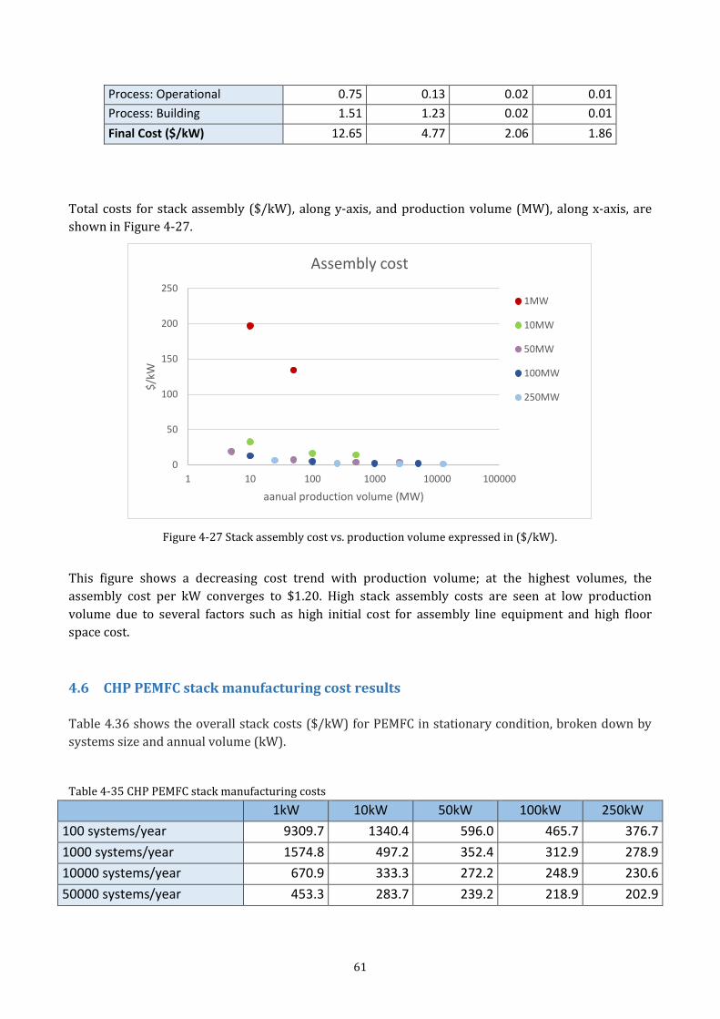
61
Process: Operational 0.75 0.13 0.02 0.01
Process: Building 1.51 1.23 0.02 0.01
Final Cost ($/kW) 12.65 4.77 2.06 1.86
Total costs for stack assembly ($/kW), along y-axis, and production volume (MW), along x-axis, are
shown in Figure 4-27.
Figure 4-27 Stack assembly cost vs. production volume expressed in ($/kW).
This figure shows a decreasing cost trend with production volume; at the highest volumes, the
assembly cost per kW converges to $1.20. High stack assembly costs are seen at low production
volume due to several factors such as high initial cost for assembly line equipment and high floor
space cost.
4.6 CHP PEMFC stack manufacturing cost results
Table 4.36 shows the overall stack costs ($/kW) for PEMFC in stationary condition, broken down by
systems size and annual volume (kW).
Table 4-35 CHP PEMFC stack manufacturing costs
1kW 10kW 50kW 100kW 250kW
100 systems/year 9309.7 1340.4 596.0 465.7 376.7
1000 systems/year 1574.8 497.2 352.4 312.9 278.9
10000 systems/year 670.9 333.3 272.2 248.9 230.6
50000 systems/year 453.3 283.7 239.2 218.9 202.9
0
50
100
150
200
250
1 10 100 1000 10000 100000
$/k
W
aanual production volume (MW)
Assembly cost
1MW
10MW
50MW
100MW
250MW
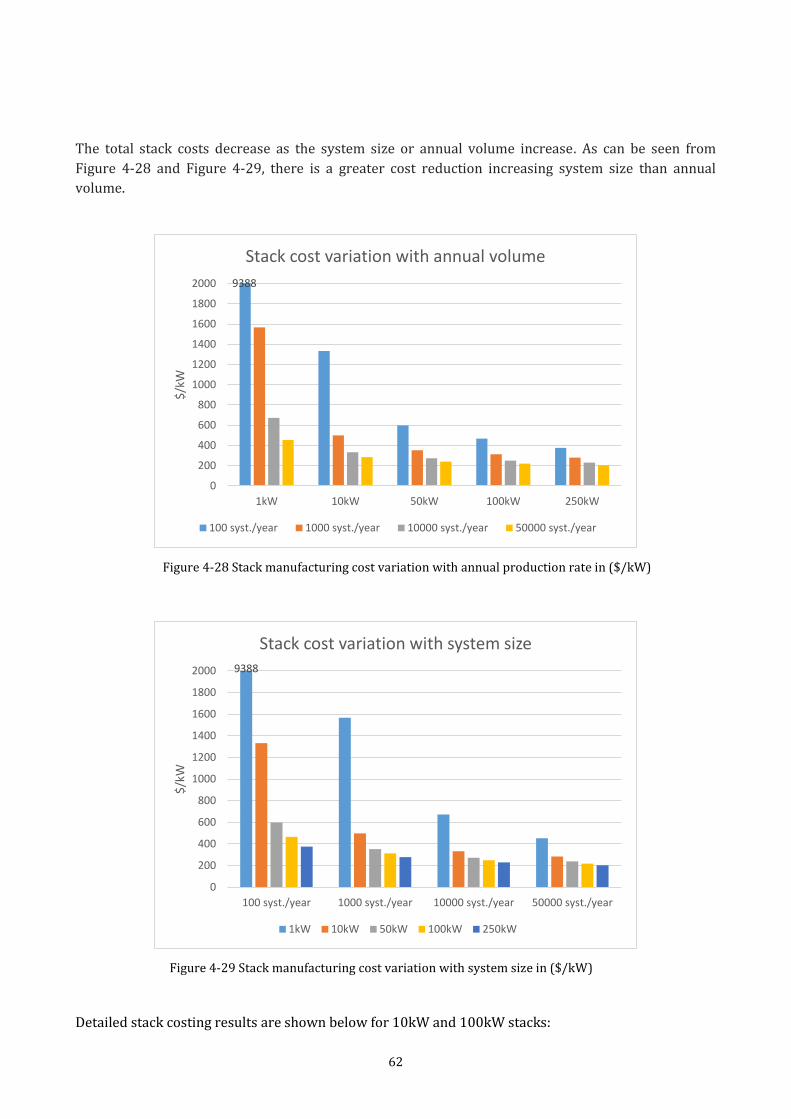
62
The total stack costs decrease as the system size or annual volume increase. As can be seen from
Figure 4-28 and Figure 4-29, there is a greater cost reduction increasing system size than annual
volume.
Figure 4-28 Stack manufacturing cost variation with annual production rate in ($/kW)
Figure 4-29 Stack manufacturing cost variation with system size in ($/kW)
Detailed stack costing results are shown below for 10kW and 100kW stacks:
9388
0
200
400
600
800
1000
1200
1400
1600
1800
2000
1kW 10kW 50kW 100kW 250kW
$/k
W
Stack cost variation with annual volume
100 syst./year 1000 syst./year 10000 syst./year 50000 syst./year
9388
0
200
400
600
800
1000
1200
1400
1600
1800
2000
100 syst./year 1000 syst./year 10000 syst./year 50000 syst./year
$/k
W
Stack cost variation with system size
1kW 10kW 50kW 100kW 250kW
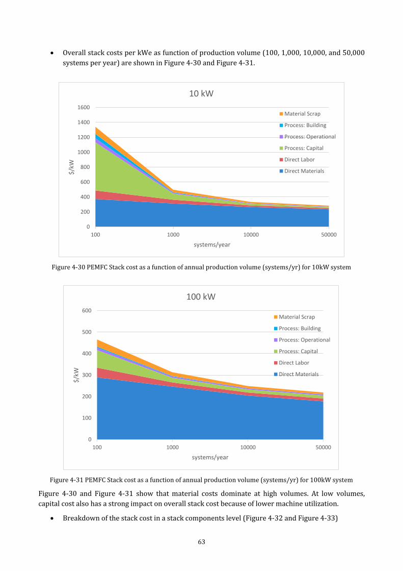
63
Overall stack costs per kWe as function of production volume (100, 1,000, 10,000, and 50,000
systems per year) are shown in Figure 4-30 and Figure 4-31.
Figure 4-30 PEMFC Stack cost as a function of annual production volume (systems/yr) for 10kW system
Figure 4-31 PEMFC Stack cost as a function of annual production volume (systems/yr) for 100kW system
Figure 4-30 and Figure 4-31 show that material costs dominate at high volumes. At low volumes,
capital cost also has a strong impact on overall stack cost because of lower machine utilization.
Breakdown of the stack cost in a stack components level (Figure 4-32 and Figure 4-33)
0
200
400
600
800
1000
1200
1400
1600
100 1000 10000 50000
$/k
W
systems/year
10 kW
Material Scrap
Process: Building
Process: Operational
Process: Capital
Direct Labor
Direct Materials
0
100
200
300
400
500
600
100 1000 10000 50000
$/k
W
systems/year
100 kW
Material Scrap
Process: Building
Process: Operational
Process: Capital
Direct Labor
Direct Materials
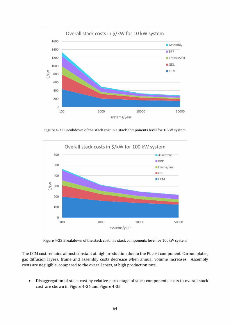
64
Figure 4-32 Breakdown of the stack cost in a stack components level for 10kW system
Figure 4-33 Breakdown of the stack cost in a stack components level for 100kW system
The CCM cost remains almost constant at high production due to the Pt cost component. Carbon plates,
gas diffusion layers, frame and assembly costs decrease when annual volume increases. Assembly
costs are negligible, compared to the overall costs, at high production rate.
Disaggregation of stack cost by relative percentage of stack components costs to overall stack
cost are shown in Figure 4-34 and Figure 4-35.
0
200
400
600
800
1000
1200
1400
1600
100 1000 10000 50000
$/k
W
systems/year
Overall stack costs in $/kW for 10 kW system
Assembly
BPP
Frame/Seal
GDL
CCM
0
100
200
300
400
500
600
100 1000 10000 50000
$/k
W
systems/year
Overall stack costs in $/kW for 100 kW system
Assembly
BPP
Frame/Seal
GDL
CCM
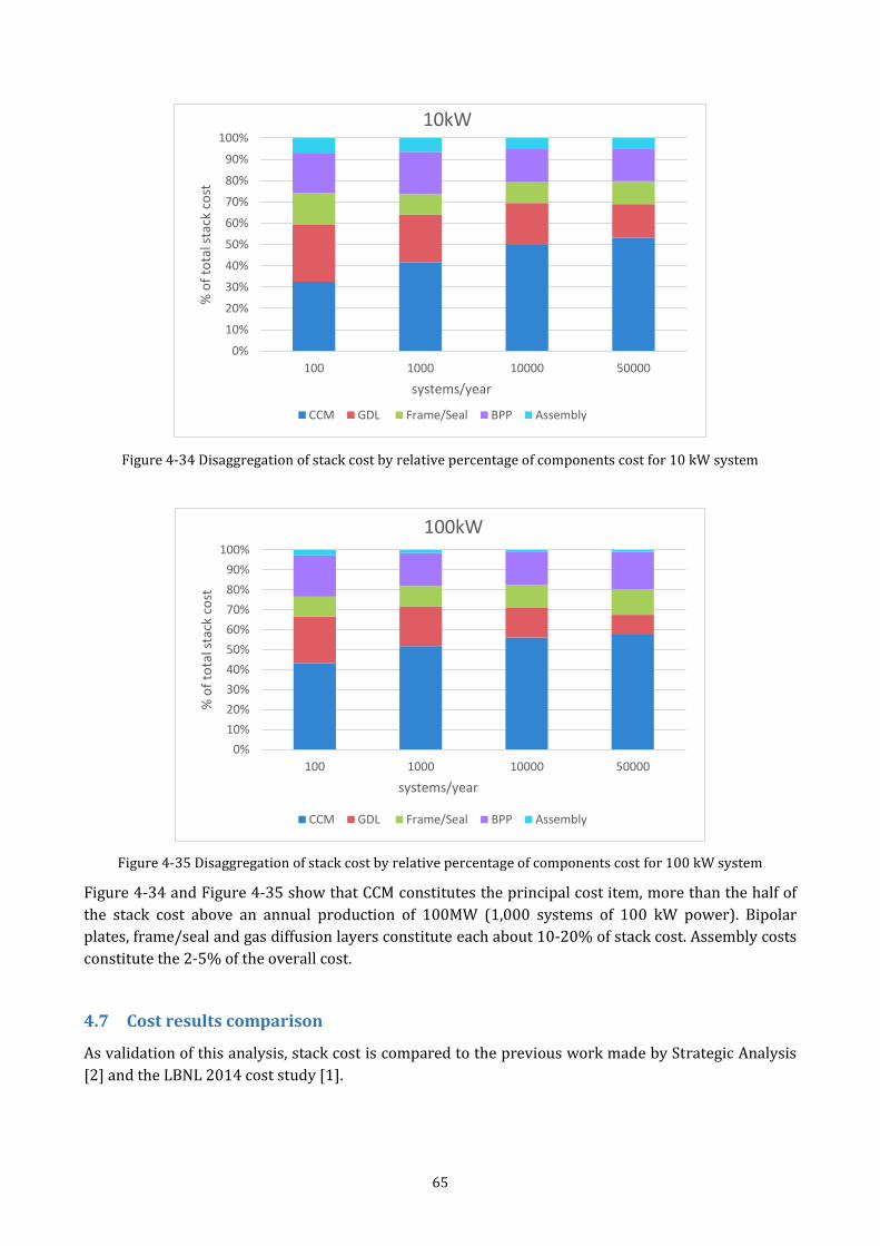
65
Figure 4-34 Disaggregation of stack cost by relative percentage of components cost for 10 kW system
Figure 4-35 Disaggregation of stack cost by relative percentage of components cost for 100 kW system
Figure 4-34 and Figure 4-35 show that CCM constitutes the principal cost item, more than the half of
the stack cost above an annual production of 100MW (1,000 systems of 100 kW power). Bipolar
plates, frame/seal and gas diffusion layers constitute each about 10-20% of stack cost. Assembly costs
constitute the 2-5% of the overall cost.
4.7 Cost results comparison
As validation of this analysis, stack cost is compared to the previous work made by Strategic Analysis
[2] and the LBNL 2014 cost study [1].
0%
10%
20%
30%
40%
50%
60%
70%
80%
90%
100%
100 1000 10000 50000
% o
f to
tal s
tack
co
st
systems/year
10kW
CCM GDL Frame/Seal BPP Assembly
0%
10%
20%
30%
40%
50%
60%
70%
80%
90%
100%
100 1000 10000 50000
% o
f to
tal s
tack
co
st
systems/year
100kW
CCM GDL Frame/Seal BPP Assembly
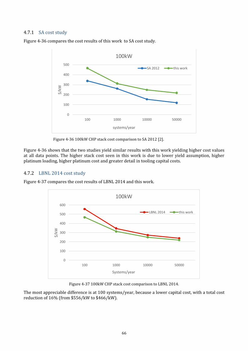
66
4.7.1 SA cost study
Figure 4-36 compares the cost results of this work to SA cost study.
Figure 4-36 100kW CHP stack cost comparison to SA 2012 [2].
Figure 4-36 shows that the two studies yield similar results with this work yielding higher cost values at all data points. The higher stack cost seen in this work is due to lower yield assumption, higher platinum loading, higher platinum cost and greater detail in tooling capital costs.
4.7.2 LBNL 2014 cost study
Figure 4-37 compares the cost results of LBNL 2014 and this work.
Figure 4-37 100kW CHP stack cost comparison to LBNL 2014.
The most appreciable difference is at 100 systems/year, because a lower capital cost, with a total cost reduction of 16% (from $556/kW to $466/kW).
0
100
200
300
400
500
100 1000 10000 50000
$/k
W
systems/year
100kW
SA 2012 this work
0
100
200
300
400
500
600
100 1000 10000 50000
$/k
W
Systems/year
100kW
LBNL 2014 this work
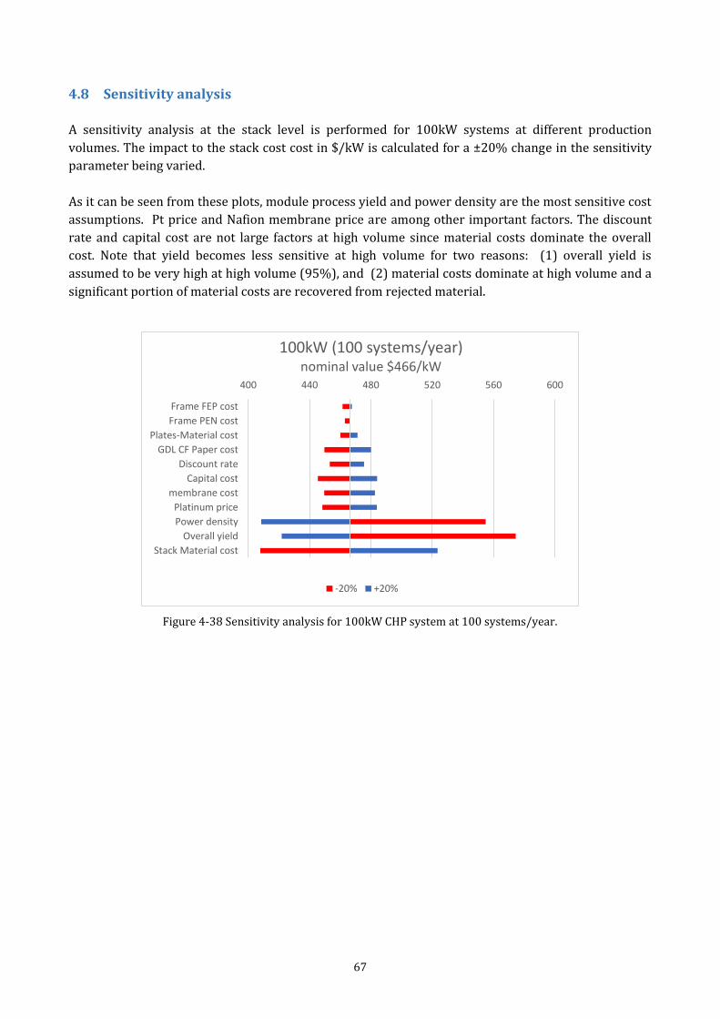
67
4.8 Sensitivity analysis
A sensitivity analysis at the stack level is performed for 100kW systems at different production
volumes. The impact to the stack cost cost in $/kW is calculated for a ±20% change in the sensitivity
parameter being varied.
As it can be seen from these plots, module process yield and power density are the most sensitive cost
assumptions. Pt price and Nafion membrane price are among other important factors. The discount
rate and capital cost are not large factors at high volume since material costs dominate the overall
cost. Note that yield becomes less sensitive at high volume for two reasons: (1) overall yield is
assumed to be very high at high volume (95%), and (2) material costs dominate at high volume and a
significant portion of material costs are recovered from rejected material.
Figure 4-38 Sensitivity analysis for 100kW CHP system at 100 systems/year.
400 440 480 520 560 600
Frame FEP cost
Frame PEN cost
Plates-Material cost
GDL CF Paper cost
Discount rate
Capital cost
membrane cost
Platinum price
Power density
Overall yield
Stack Material cost
100kW (100 systems/year) nominal value $466/kW
-20% +20%
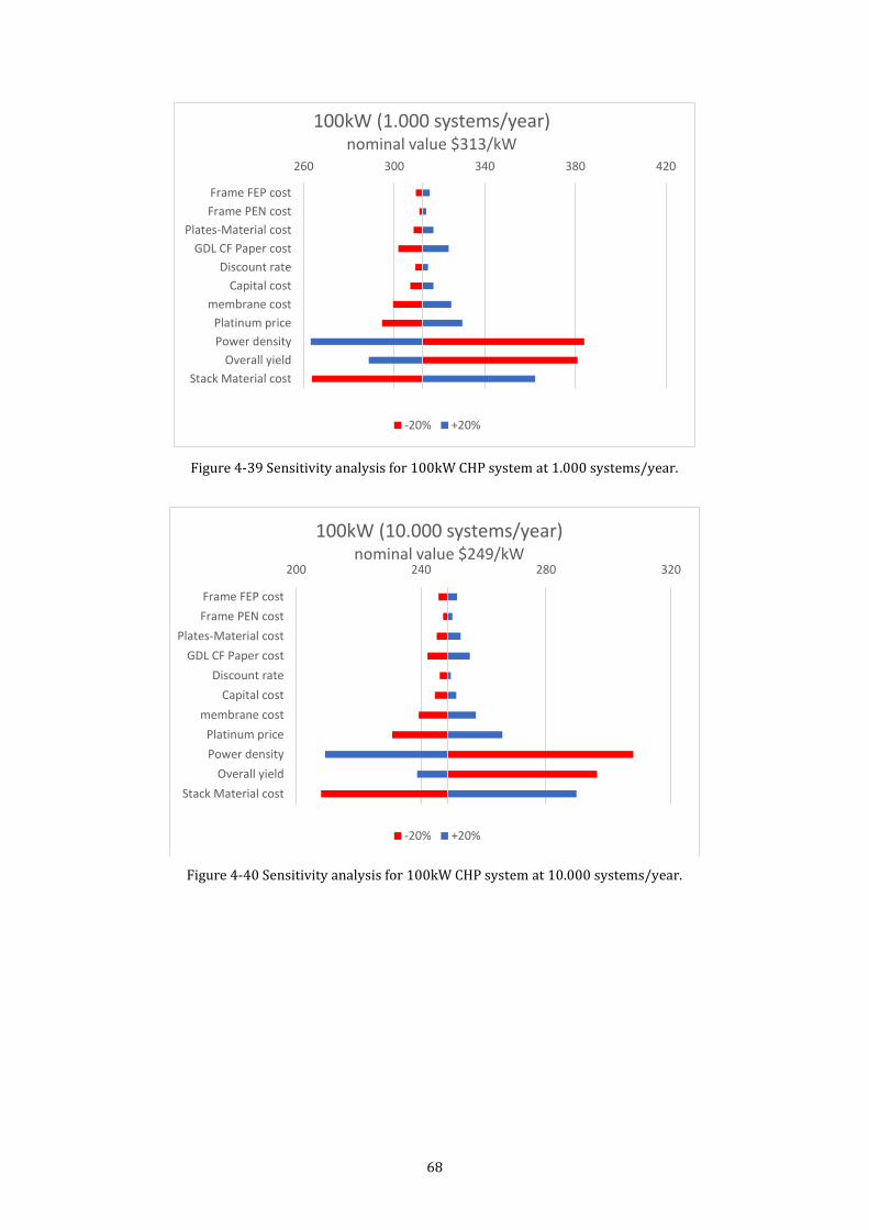
68
Figure 4-39 Sensitivity analysis for 100kW CHP system at 1.000 systems/year.
Figure 4-40 Sensitivity analysis for 100kW CHP system at 10.000 systems/year.
260 300 340 380 420
Frame FEP cost
Frame PEN cost
Plates-Material cost
GDL CF Paper cost
Discount rate
Capital cost
membrane cost
Platinum price
Power density
Overall yield
Stack Material cost
100kW (1.000 systems/year) nominal value $313/kW
-20% +20%
200 240 280 320
Frame FEP cost
Frame PEN cost
Plates-Material cost
GDL CF Paper cost
Discount rate
Capital cost
membrane cost
Platinum price
Power density
Overall yield
Stack Material cost
100kW (10.000 systems/year) nominal value $249/kW
-20% +20%
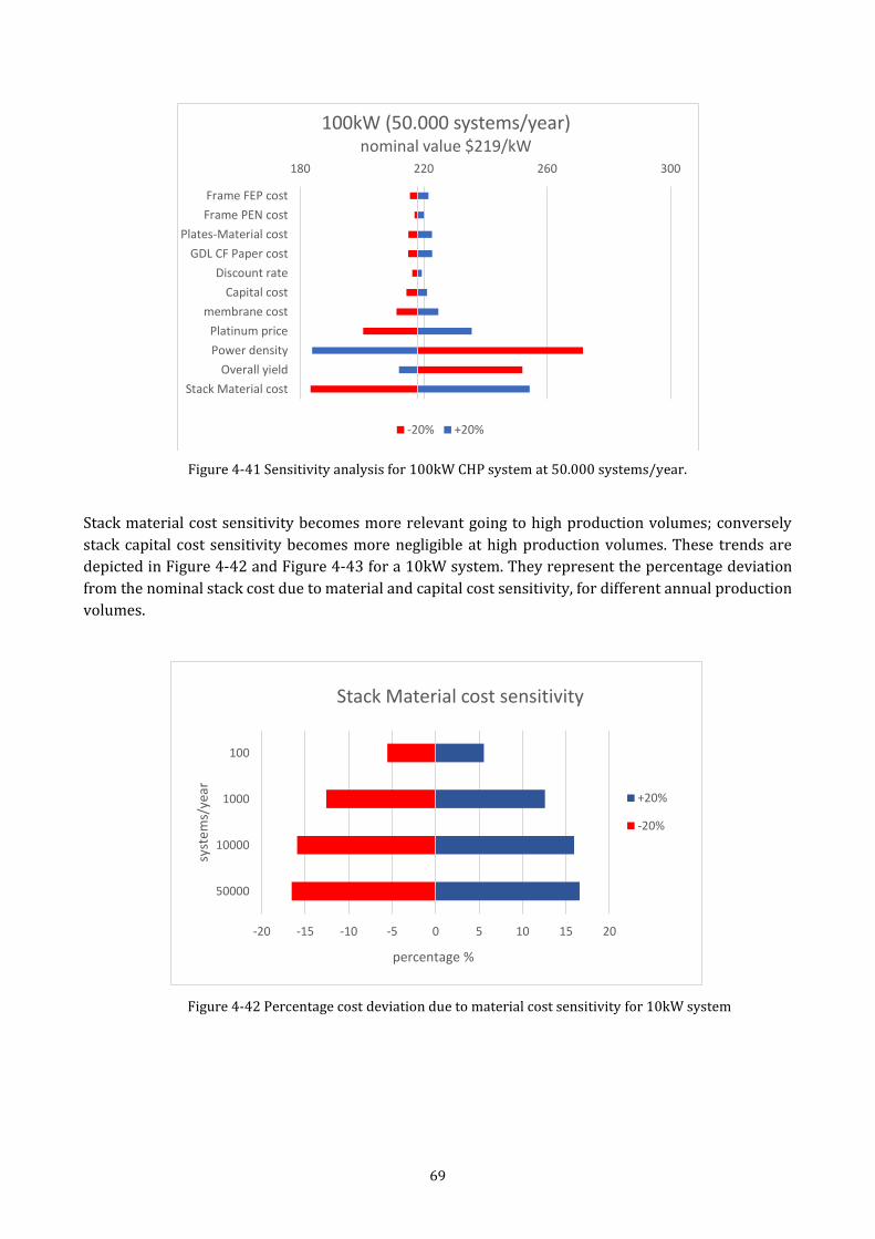
69
Figure 4-41 Sensitivity analysis for 100kW CHP system at 50.000 systems/year.
Stack material cost sensitivity becomes more relevant going to high production volumes; conversely
stack capital cost sensitivity becomes more negligible at high production volumes. These trends are
depicted in Figure 4-42 and Figure 4-43 for a 10kW system. They represent the percentage deviation
from the nominal stack cost due to material and capital cost sensitivity, for different annual production
volumes.
Figure 4-42 Percentage cost deviation due to material cost sensitivity for 10kW system
180 220 260 300
Frame FEP cost
Frame PEN cost
Plates-Material cost
GDL CF Paper cost
Discount rate
Capital cost
membrane cost
Platinum price
Power density
Overall yield
Stack Material cost
100kW (50.000 systems/year) nominal value $219/kW
-20% +20%
-20 -15 -10 -5 0 5 10 15 20
100
1000
10000
50000
percentage %
syst
ems/
year
Stack Material cost sensitivity
+20%
-20%
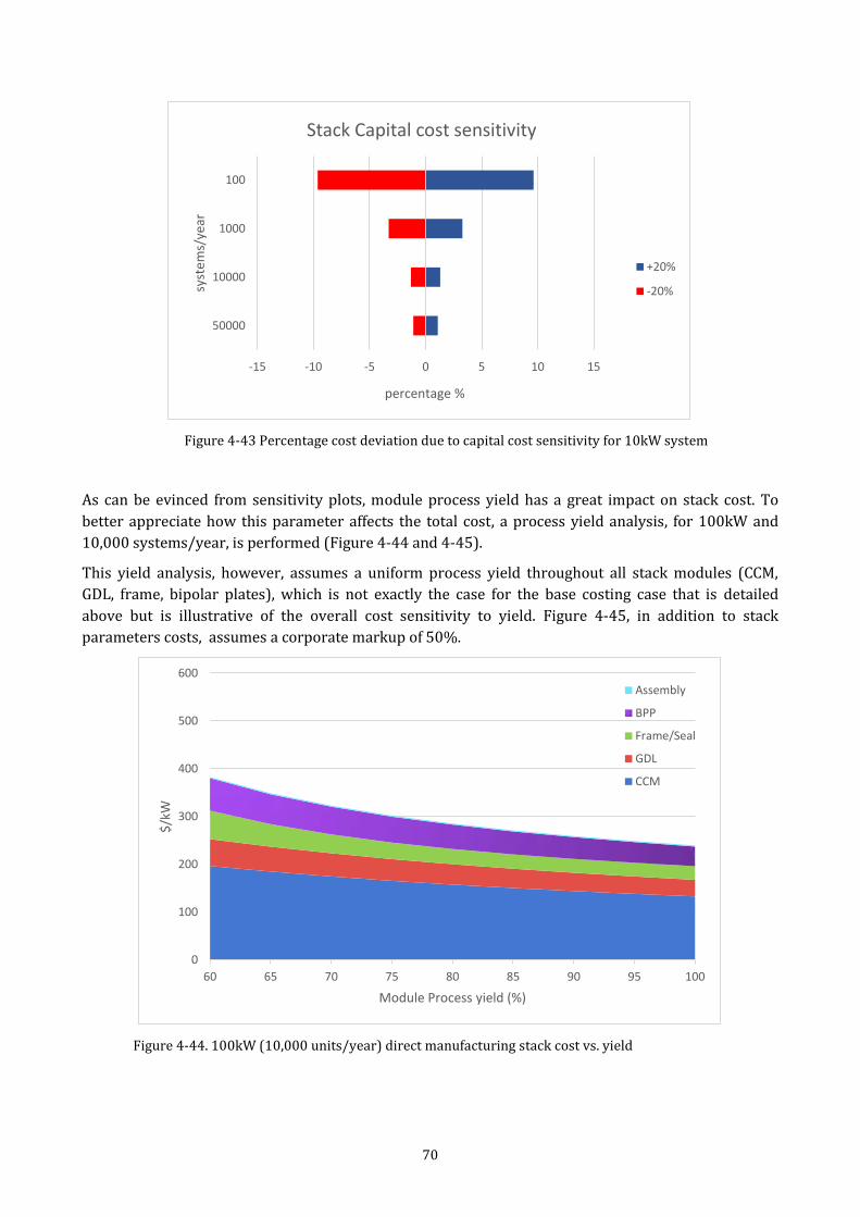
70
Figure 4-43 Percentage cost deviation due to capital cost sensitivity for 10kW system
As can be evinced from sensitivity plots, module process yield has a great impact on stack cost. To
better appreciate how this parameter affects the total cost, a process yield analysis, for 100kW and
10,000 systems/year, is performed (Figure 4-44 and 4-45).
This yield analysis, however, assumes a uniform process yield throughout all stack modules (CCM,
GDL, frame, bipolar plates), which is not exactly the case for the base costing case that is detailed
above but is illustrative of the overall cost sensitivity to yield. Figure 4-45, in addition to stack
parameters costs, assumes a corporate markup of 50%.
Figure 4-44. 100kW (10,000 units/year) direct manufacturing stack cost vs. yield
-15 -10 -5 0 5 10 15
100
1000
10000
50000
percentage %
syst
ems/
year
Stack Capital cost sensitivity
+20%
-20%
0
100
200
300
400
500
600
60 65 70 75 80 85 90 95 100
$/k
W
Module Process yield (%)
Assembly
BPP
Frame/Seal
GDL
CCM
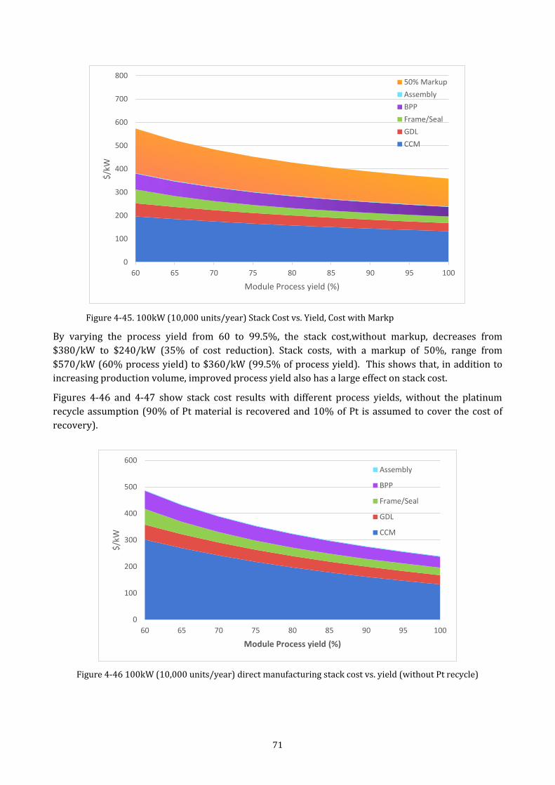
71
Figure 4-45. 100kW (10,000 units/year) Stack Cost vs. Yield, Cost with Markp
By varying the process yield from 60 to 99.5%, the stack cost,without markup, decreases from
$380/kW to $240/kW (35% of cost reduction). Stack costs, with a markup of 50%, range from
$570/kW (60% process yield) to $360/kW (99.5% of process yield). This shows that, in addition to
increasing production volume, improved process yield also has a large effect on stack cost.
Figures 4-46 and 4-47 show stack cost results with different process yields, without the platinum
recycle assumption (90% of Pt material is recovered and 10% of Pt is assumed to cover the cost of
recovery).
Figure 4-46 100kW (10,000 units/year) direct manufacturing stack cost vs. yield (without Pt recycle)
0
100
200
300
400
500
600
700
800
60 65 70 75 80 85 90 95 100
$/k
W
Module Process yield (%)
50% Markup
Assembly
BPP
Frame/Seal
GDL
CCM
0
100
200
300
400
500
600
60 65 70 75 80 85 90 95 100
$/k
W
Module Process yield (%)
Assembly
BPP
Frame/Seal
GDL
CCM
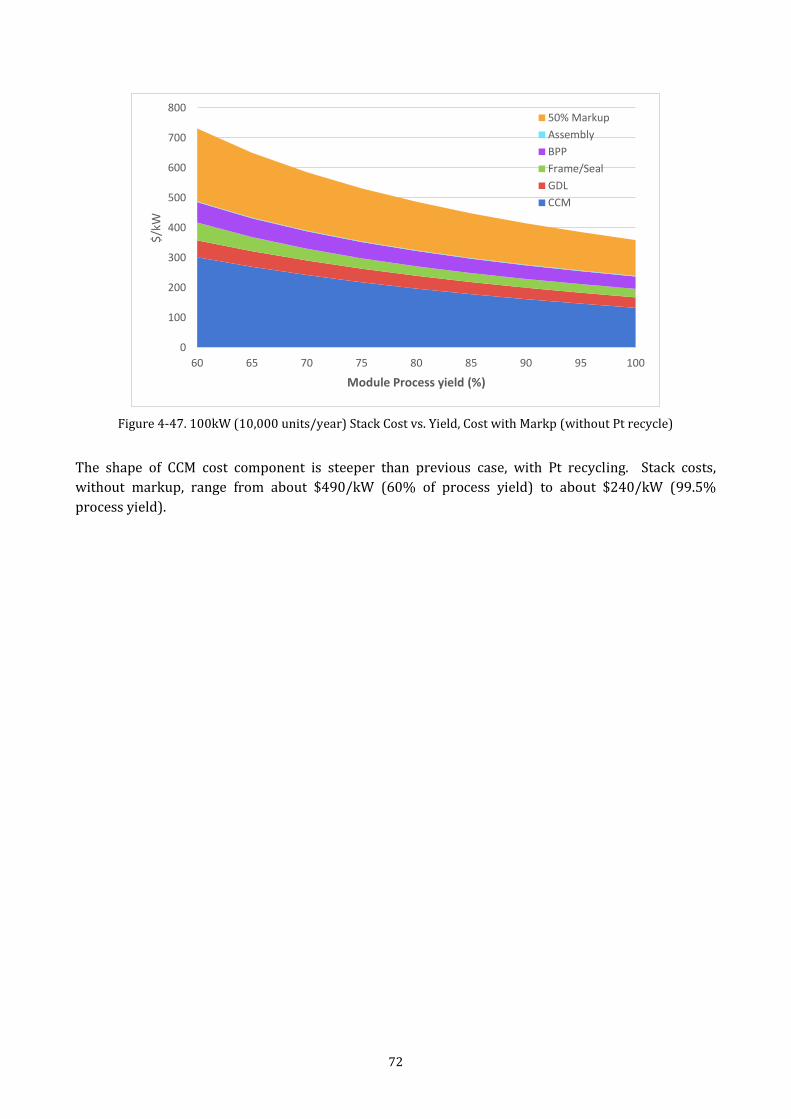
72
Figure 4-47. 100kW (10,000 units/year) Stack Cost vs. Yield, Cost with Markp (without Pt recycle)
The shape of CCM cost component is steeper than previous case, with Pt recycling. Stack costs,
without markup, range from about $490/kW (60% of process yield) to about $240/kW (99.5%
process yield).
0
100
200
300
400
500
600
700
800
60 65 70 75 80 85 90 95 100
$/k
W
Module Process yield (%)
50% Markup
Assembly
BPP
Frame/Seal
GDL
CCM
73
5 Balance Of Plant and System Costs
This chapter analyzes the balance of plant of a PEMFC system and compares the total system cost to
DOE targets. The fuel cell system (FCS) consists primarily of the fuel cell stack and the balance of plant
(BOP) components. The BOP includes items such as valves, compressors, pumps, wiring, piping,
meters, controls etc. that are associated with the complete operation of the fuel cell system.
Six major areas make up the BOP and are listed below:
- Fuel Processing Subsystem
The fuel processing subsystem consists of a fuel processor for producing hydrogen fuel from natural
gas. The fuel processing subsystem is comprised of components associated with the operation of the
fuel reformer, which includes parts such as sensors, controls, filters, pumps, and valves.
- Air Subsystem
The air subsystem consists of components associated with oxidant delivery to the fuel cell stack. Major
components in this subsystem are storage tanks, compressor, motor, piping, and manifolds.
- Coolant and Humidification Subsystems
The coolant subsystem consists of components associated with water management in the FCS,
including humidification of membranes. These include: tank, pump motor, piping and external cooling
motor.
- Power Subsystem
The power subsystem contains components required for powering the system and conditioning the
output power. The system includes: inverter, transistor, transformer, power supply, relays, switches,
fuses, resistors, Human Machine Interface (HMI), amplifiers, and cables.
- Controls and Meters Subsystem
This controls and meters subsystem contains system controls-related components for system
operation and equipment monitoring. This subsystem includes items such as the variable frequency
drive (VFD), sensors, meters, and virtual private network (VPN) system.
- Miscellaneous Subsystem
The miscellaneous subsystem comprises external items outside of the stack that provides support,
structure, and protection for the FCS. These items include: tubing, enclosure, fasteners, fire/safety
panels, and labor.
- Thermal management
The thermal management consists of the heat exchangers, for for water heating and space heating, and
the condenser.
5.1 Balance of plant results
Table 5-1 displays the component breakdown of BOP subsystem costs for the 10kW and 100kW CHP
system with reformate fuel at production volume of 1.000 systems per year. For the 100kW CHP
system, the external cooling motor dominates the coolant subsystem, accounting for approximately
half of the subsystem cost. The cost of the power subsystem is dominated by the power inverter, which
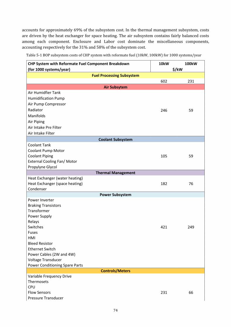
74
accounts for approximately 69% of the subsystem cost. In the thermal management subsystem, costs
are driven by the heat exchanger for space heating. The air subsystem contains fairly balanced costs
among each component. Enclosure and Labor cost dominate the miscellaneous components,
accounting respectively for the 31% and 58% of the subsystem cost.
Table 5-1 BOP subsystem costs of CHP system with reformate fuel (10kW, 100kW) for 1000 systems/year
CHP System with Reformate Fuel Component Breakdown 10kW 100kW
(for 1000 systems/year) $/kW
Fuel Processing Subsystem
602 231
Air Subsytem
Air Humidfier Tank
Humidification Pump
Air Pump Compressor
Radiator 246 59
Manifolds
Air Piping
Air Intake Pre Filter
Air Intake Filter
Coolant Subsystem
Coolant Tank
Coolant Pump Motor
Coolant Piping 105 59 External Cooling Fan/ Motor
Propylyne Glycol
Thermal Management
Heat Exchanger (water heating)
Heat Exchanger (space heating) 182 76 Condenser
Power Subsystem Power Inverter
Braking Transistors
Transformer
Power Supply
Relays
Switches 421 249 Fuses
HMI
Bleed Resistor
Ethernet Switch
Power Cables (2W and 4W)
Voltage Transducer
Power Conditioning Spare Parts
Controls/Meters
Variable Frequency Drive
Thermosets
CPU
Flow Sensors 231 66
Pressure Transducer
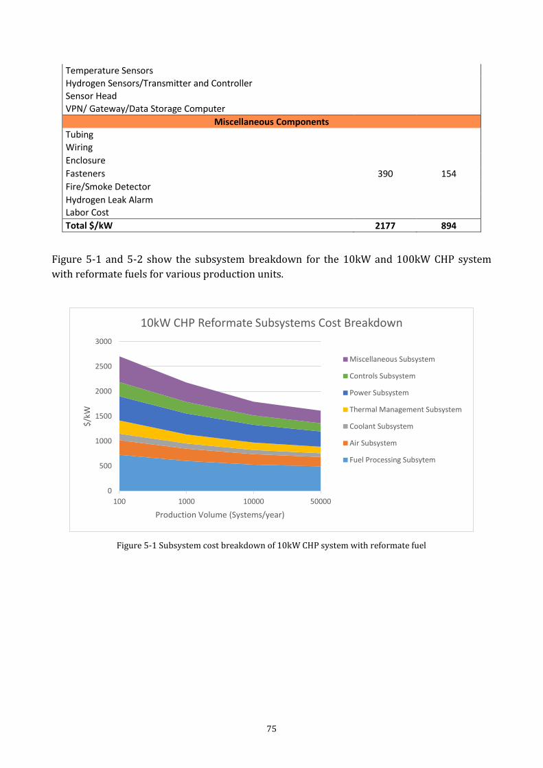
75
Temperature Sensors
Hydrogen Sensors/Transmitter and Controller
Sensor Head
VPN/ Gateway/Data Storage Computer
Miscellaneous Components
Tubing
Wiring
Enclosure
Fasteners 390 154
Fire/Smoke Detector
Hydrogen Leak Alarm
Labor Cost
Total $/kW 2177 894
Figure 5-1 and 5-2 show the subsystem breakdown for the 10kW and 100kW CHP system
with reformate fuels for various production units.
Figure 5-1 Subsystem cost breakdown of 10kW CHP system with reformate fuel
0
500
1000
1500
2000
2500
3000
100 1000 10000 50000
$/k
W
Production Volume (Systems/year)
10kW CHP Reformate Subsystems Cost Breakdown
Miscellaneous Subsystem
Controls Subsystem
Power Subsystem
Thermal Management Subsystem
Coolant Subsystem
Air Subsystem
Fuel Processing Subsytem
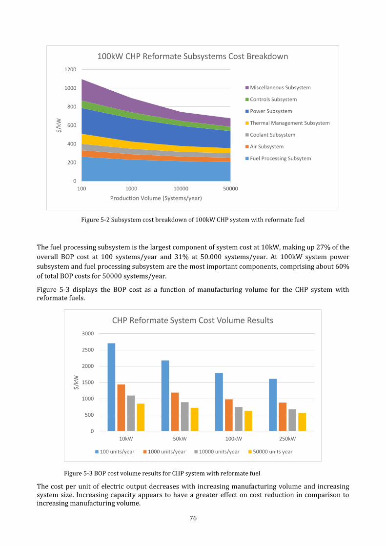
76
Figure 5-2 Subsystem cost breakdown of 100kW CHP system with reformate fuel
The fuel processing subsystem is the largest component of system cost at 10kW, making up 27% of the
overall BOP cost at 100 systems/year and 31% at 50.000 systems/year. At 100kW system power
subsystem and fuel processing subsystem are the most important components, comprising about 60%
of total BOP costs for 50000 systems/year.
Figure 5-3 displays the BOP cost as a function of manufacturing volume for the CHP system with reformate fuels.
Figure 5-3 BOP cost volume results for CHP system with reformate fuel
The cost per unit of electric output decreases with increasing manufacturing volume and increasing system size. Increasing capacity appears to have a greater effect on cost reduction in comparison to increasing manufacturing volume.
0
200
400
600
800
1000
1200
100 1000 10000 50000
$/k
W
Production Volume (Systems/year)
100kW CHP Reformate Subsystems Cost Breakdown
Miscellaneous Subsystem
Controls Subsystem
Power Subsystem
Thermal Management Subsystem
Coolant Subsystem
Air Subsystem
Fuel Processing Subsytem
0
500
1000
1500
2000
2500
3000
10kW 50kW 100kW 250kW
$/k
W
CHP Reformate System Cost Volume Results
100 units/year 1000 units/year 10000 units/year 50000 units year
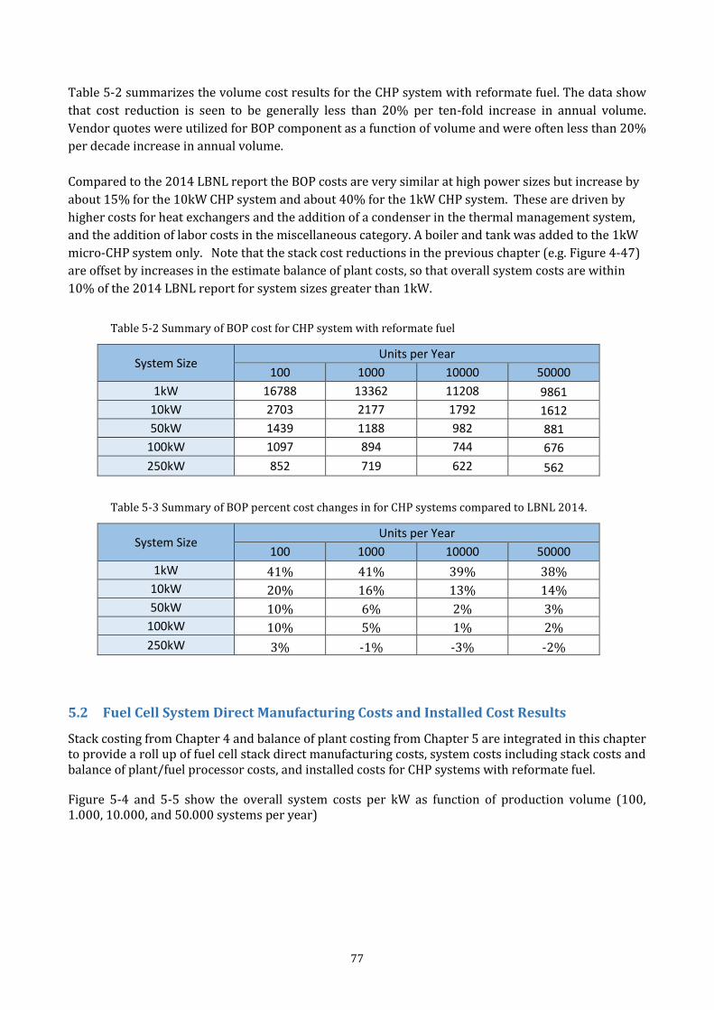
77
Table 5-2 summarizes the volume cost results for the CHP system with reformate fuel. The data show
that cost reduction is seen to be generally less than 20% per ten-fold increase in annual volume.
Vendor quotes were utilized for BOP component as a function of volume and were often less than 20%
per decade increase in annual volume.
Compared to the 2014 LBNL report the BOP costs are very similar at high power sizes but increase by
about 15% for the 10kW CHP system and about 40% for the 1kW CHP system. These are driven by
higher costs for heat exchangers and the addition of a condenser in the thermal management system,
and the addition of labor costs in the miscellaneous category. A boiler and tank was added to the 1kW
micro-CHP system only. Note that the stack cost reductions in the previous chapter (e.g. Figure 4-47)
are offset by increases in the estimate balance of plant costs, so that overall system costs are within
10% of the 2014 LBNL report for system sizes greater than 1kW.
Table 5-2 Summary of BOP cost for CHP system with reformate fuel
System Size Units per Year
100 1000 10000 50000
1kW 16788 13362 11208 9861
10kW 2703 2177 1792 1612
50kW 1439 1188 982 881
100kW 1097 894 744 676
250kW 852 719 622 562
Table 5-3 Summary of BOP percent cost changes in for CHP systems compared to LBNL 2014.
System Size Units per Year
100 1000 10000 50000
1kW 41% 41% 39% 38%
10kW 20% 16% 13% 14%
50kW 10% 6% 2% 3%
100kW 10% 5% 1% 2%
250kW 3% -1% -3% -2%
5.2 Fuel Cell System Direct Manufacturing Costs and Installed Cost Results
Stack costing from Chapter 4 and balance of plant costing from Chapter 5 are integrated in this chapter to provide a roll up of fuel cell stack direct manufacturing costs, system costs including stack costs and balance of plant/fuel processor costs, and installed costs for CHP systems with reformate fuel.
Figure 5-4 and 5-5 show the overall system costs per kW as function of production volume (100, 1.000, 10.000, and 50.000 systems per year)
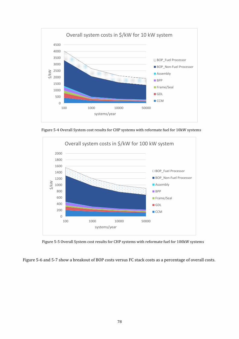
78
Figure 5-4 Overall System cost results for CHP systems with reformate fuel for 10kW systems
Figure 5-5 Overall System cost results for CHP systems with reformate fuel for 100kW systems
Figure 5-6 and 5-7 show a breakout of BOP costs versus FC stack costs as a percentage of overall costs.
0
500
1000
1500
2000
2500
3000
3500
4000
4500
100 1000 10000 50000
$/k
W
systems/year
Overall system costs in $/kW for 10 kW system
BOP_Fuel Processor
BOP_Non-Fuel Processor
Assembly
BPP
Frame/Seal
GDL
CCM
0
200
400
600
800
1000
1200
1400
1600
1800
2000
100 1000 10000 50000
$/k
W
systems/year
Overall system costs in $/kW for 100 kW system
BOP_Fuel Processor
BOP_Non-Fuel Processor
Assembly
BPP
Frame/Seal
GDL
CCM
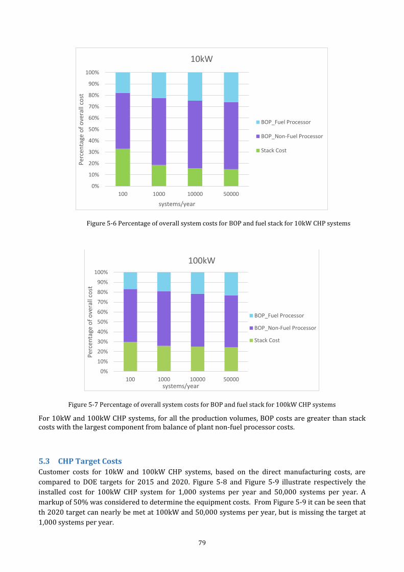
79
Figure 5-6 Percentage of overall system costs for BOP and fuel stack for 10kW CHP systems
Figure 5-7 Percentage of overall system costs for BOP and fuel stack for 100kW CHP systems
For 10kW and 100kW CHP systems, for all the production volumes, BOP costs are greater than stack costs with the largest component from balance of plant non-fuel processor costs.
5.3 CHP Target Costs
Customer costs for 10kW and 100kW CHP systems, based on the direct manufacturing costs, are
compared to DOE targets for 2015 and 2020. Figure 5-8 and Figure 5-9 illustrate respectively the
installed cost for 100kW CHP system for 1,000 systems per year and 50,000 systems per year. A
markup of 50% was considered to determine the equipment costs. From Figure 5-9 it can be seen that
th 2020 target can nearly be met at 100kW and 50,000 systems per year, but is missing the target at
1,000 systems per year.
0%
10%
20%
30%
40%
50%
60%
70%
80%
90%
100%
100 1000 10000 50000
Per
cen
tage
of
ove
rall
cost
systems/year
10kW
BOP_Fuel Processor
BOP_Non-Fuel Processor
Stack Cost
0%
10%
20%
30%
40%
50%
60%
70%
80%
90%
100%
100 1000 10000 50000
Per
cen
tage
of
ove
rall
cost
systems/year
100kW
BOP_Fuel Processor
BOP_Non-Fuel Processor
Stack Cost
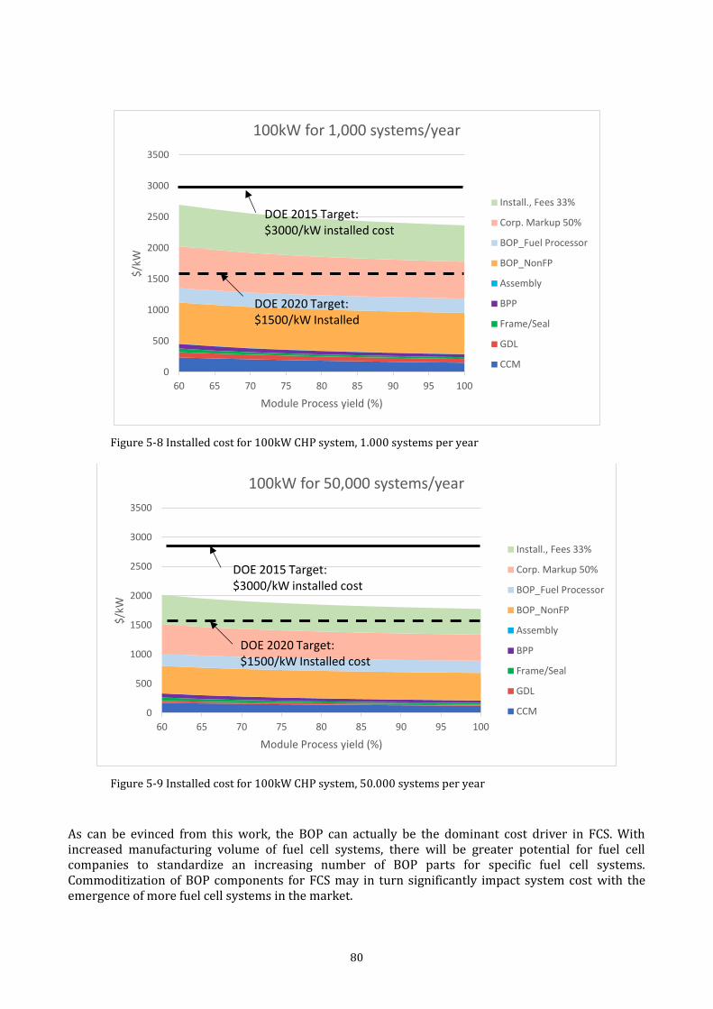
80
Figure 5-8 Installed cost for 100kW CHP system, 1.000 systems per year
Figure 5-9 Installed cost for 100kW CHP system, 50.000 systems per year
As can be evinced from this work, the BOP can actually be the dominant cost driver in FCS. With increased manufacturing volume of fuel cell systems, there will be greater potential for fuel cell companies to standardize an increasing number of BOP parts for specific fuel cell systems. Commoditization of BOP components for FCS may in turn significantly impact system cost with the emergence of more fuel cell systems in the market.
0
500
1000
1500
2000
2500
3000
3500
60 65 70 75 80 85 90 95 100
$/k
W
Module Process yield (%)
100kW for 1,000 systems/year
Install., Fees 33%
Corp. Markup 50%
BOP_Fuel Processor
BOP_NonFP
Assembly
BPP
Frame/Seal
GDL
CCM
DOE 2015 Target: $3000/kW installed cost
DOE 2020 Target: $1500/kW Installed
0
500
1000
1500
2000
2500
3000
3500
60 65 70 75 80 85 90 95 100
$/k
W
Module Process yield (%)
100kW for 50,000 systems/year
Install., Fees 33%
Corp. Markup 50%
BOP_Fuel Processor
BOP_NonFP
Assembly
BPP
Frame/Seal
GDL
CCM
DOE 2015 Target: $3000/kW installed cost
DOE 2020 Target: $1500/kW Installed cost
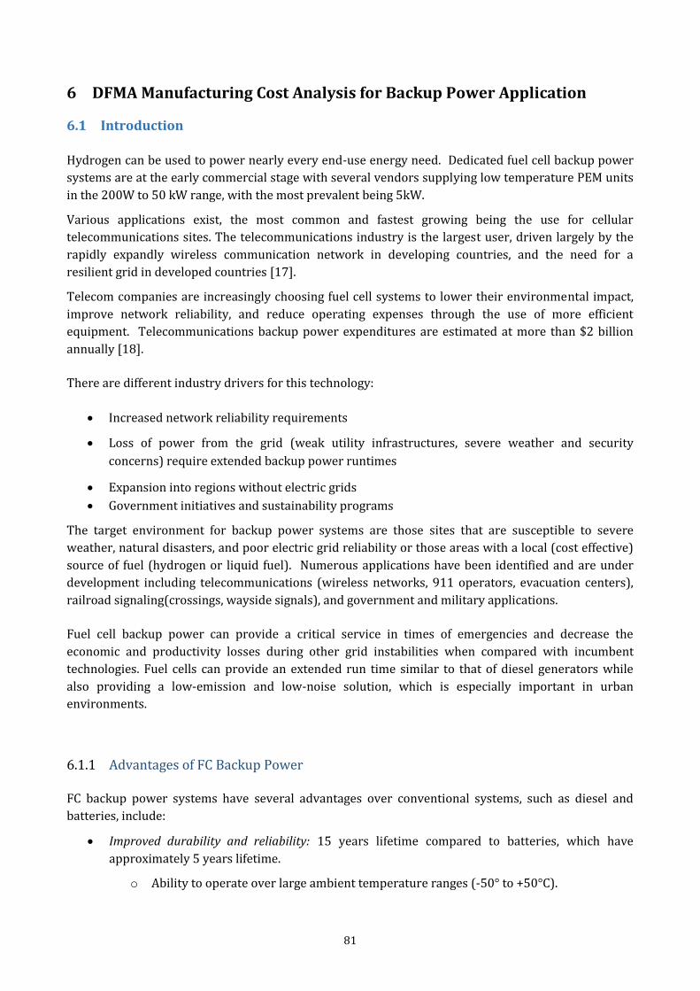
81
6 DFMA Manufacturing Cost Analysis for Backup Power Application
6.1 Introduction
Hydrogen can be used to power nearly every end-use energy need. Dedicated fuel cell backup power
systems are at the early commercial stage with several vendors supplying low temperature PEM units
in the 200W to 50 kW range, with the most prevalent being 5kW.
Various applications exist, the most common and fastest growing being the use for cellular
telecommunications sites. The telecommunications industry is the largest user, driven largely by the
rapidly expandly wireless communication network in developing countries, and the need for a
resilient grid in developed countries [17].
Telecom companies are increasingly choosing fuel cell systems to lower their environmental impact,
improve network reliability, and reduce operating expenses through the use of more efficient
equipment. Telecommunications backup power expenditures are estimated at more than $2 billion
annually [18].
There are different industry drivers for this technology:
Increased network reliability requirements
Loss of power from the grid (weak utility infrastructures, severe weather and security
concerns) require extended backup power runtimes
Expansion into regions without electric grids
Government initiatives and sustainability programs
The target environment for backup power systems are those sites that are susceptible to severe
weather, natural disasters, and poor electric grid reliability or those areas with a local (cost effective)
source of fuel (hydrogen or liquid fuel). Numerous applications have been identified and are under
development including telecommunications (wireless networks, 911 operators, evacuation centers),
railroad signaling(crossings, wayside signals), and government and military applications.
Fuel cell backup power can provide a critical service in times of emergencies and decrease the
economic and productivity losses during other grid instabilities when compared with incumbent
technologies. Fuel cells can provide an extended run time similar to that of diesel generators while
also providing a low-emission and low-noise solution, which is especially important in urban
environments.
6.1.1 Advantages of FC Backup Power
FC backup power systems have several advantages over conventional systems, such as diesel and
batteries, include:
Improved durability and reliability: 15 years lifetime compared to batteries, which have
approximately 5 years lifetime.
o Ability to operate over large ambient temperature ranges (-50° to +50°C).
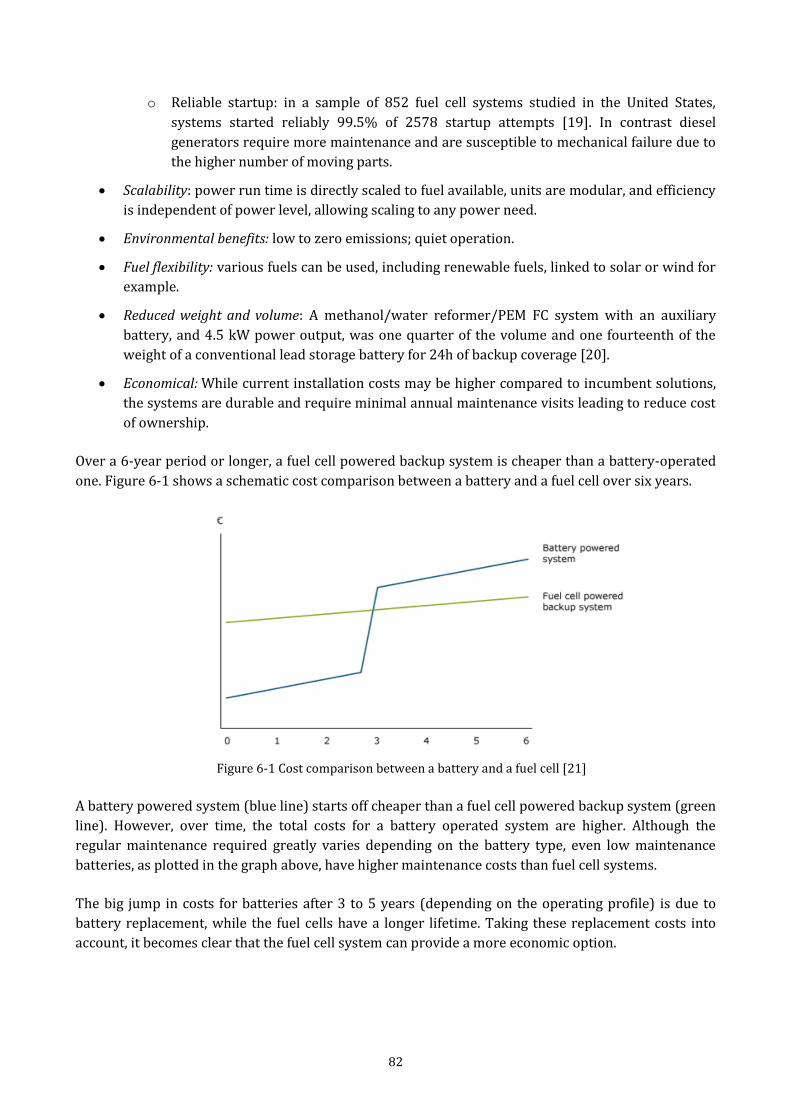
82
o Reliable startup: in a sample of 852 fuel cell systems studied in the United States,
systems started reliably 99.5% of 2578 startup attempts [19]. In contrast diesel
generators require more maintenance and are susceptible to mechanical failure due to
the higher number of moving parts.
Scalability: power run time is directly scaled to fuel available, units are modular, and efficiency
is independent of power level, allowing scaling to any power need.
Environmental benefits: low to zero emissions; quiet operation.
Fuel flexibility: various fuels can be used, including renewable fuels, linked to solar or wind for
example.
Reduced weight and volume: A methanol/water reformer/PEM FC system with an auxiliary
battery, and 4.5 kW power output, was one quarter of the volume and one fourteenth of the
weight of a conventional lead storage battery for 24h of backup coverage [20].
Economical: While current installation costs may be higher compared to incumbent solutions,
the systems are durable and require minimal annual maintenance visits leading to reduce cost
of ownership.
Over a 6-year period or longer, a fuel cell powered backup system is cheaper than a battery-operated
one. Figure 6-1 shows a schematic cost comparison between a battery and a fuel cell over six years.
Figure 6-1 Cost comparison between a battery and a fuel cell [21]
A battery powered system (blue line) starts off cheaper than a fuel cell powered backup system (green
line). However, over time, the total costs for a battery operated system are higher. Although the
regular maintenance required greatly varies depending on the battery type, even low maintenance
batteries, as plotted in the graph above, have higher maintenance costs than fuel cell systems.
The big jump in costs for batteries after 3 to 5 years (depending on the operating profile) is due to
battery replacement, while the fuel cells have a longer lifetime. Taking these replacement costs into
account, it becomes clear that the fuel cell system can provide a more economic option.

83
6.1.2 Fuel cell backup power system design The fuel cell backup power plant consists of three major components:
Hydrogen Storage Fuel Cell Stack Battery/Capacitor
Hydrogen Storage
Fuel cell installations are typically fueled by a six-pack of compressed hydrogen storage containers.
These containers each hold either 139 scf (standard cubic foot) or 261 scf of hydrogen at a pressure of
2,400 psi and a weight of 137 lbs. They have the combined capacity to power a fuel cell for 24–96
hours [22]
Fuel Cell Stack
A single fuel cell will not provide the required power for most applications. Therefore, multiple fuel
cells, referred to as a stack, are linked together in a fuel cell power plant to meet the required power
demand.
Battery/Capacitor
Fuel cell power plants used for backup power typically require a DC storage device to provide
immediate power while the fuel cell powers up. PEM fuel cells power up quickly, but there is still a
short period of time that requires the use of a battery or capacitor to supply power.
Telecommunications installations with backup fuel cell power often incorporate fuel cells and
batteries. As the system voltage changes, rectifiers or controllers switch between the primary power
source and the backup power sources.
In the absence of grid power or another primary alternating current (AC) power source, the fuel cells,
or a combination of fuel cells and batteries, provide direct current (DC) power to run the equipment.
The fuel cells have internal batteries that provide temporary “bridge” power until the fuel cell reaches
peak power production and takes over the load. When the primary power source is restored, the fuel
cells shut down, and the load is returned to the primary source.
Figure 6-2 shows a fuel cell backup power system design.
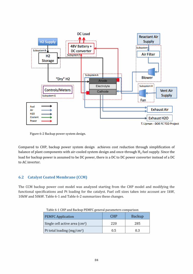
84
Figure 6-2 Backup power system design.
Compared to CHP, backup power system design achieves cost reduction through simplification of
balance of plant components with air-cooled system design and once-through H2 fuel supply. Since the
load for backup power is assumed to be DC power, there is a DC to DC power converter instead of a DC
to AC inverter.
6.2 Catalyst Coated Membrane (CCM)
The CCM backup power cost model was analyzed starting from the CHP model and modifying the
functional specifications and Pt loading for the catalyst. Fuel cell sizes taken into account are 1kW,
10kW and 50kW. Table 6-1 and Table 6-2 summarizes these changes.
Table 6-1 CHP and Backup PEMFC general parameters comparison
PEMFC Application CHP Backup
Single cell active area (cm2) 220 285
Pt total loading (mg/cm2) 0.5 0.3
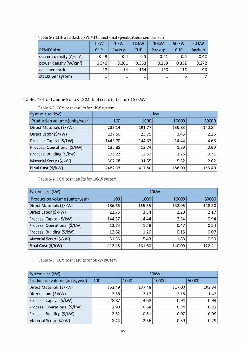
85
Table 6-2 CHP and Backup PEMFC functional specifications comparison
PEMFC size
1 kW
CHP
1 kW
Backup
10 kW
CHP
10kW
Backup
50 kW
CHP
50 kW
Backup
current density (A/cm2) 0.49 0.4 0.5 0.41 0.5 0.42
power density (W/cm2) 0.346 0.261 0.353 0.269 0.352 0.272
cells per stack 17 14 164 136 136 96
stacks per system 1 1 1 1 6 7
Tables 6-3, 6-4 and 6-5 show CCM final costs in terms of $/kW.
Table 6-3 CCM cost results for 1kW system
System size (kW) 1kW
Production volume (units/year) 100 1000 10000 50000
Direct Materials ($/kW) 235.14 191.77 159.83 142.84
Direct Labor ($/kW) 237.50 23.75 3.45 2.26
Process: Capital ($/kW) 1443.70 144.37 14.44 4.68
Process: Operational ($/kW) 132.38 13.74 1.59 0.69
Process: Building ($/kW) 126.22 12.62 1.26 0.31
Material Scrap ($/kW) 307.08 31.55 5.52 2.62
Final Cost ($/kW) 2482.03 417.80 186.09 153.40
Table 6-4 CCM cost results for 10kW system
Table 6-5 CCM cost results for 50kW system
System size (kW) 10kW
Production volume (units/year) 100 1000 10000 50000
Direct Materials ($/kW) 186.66 155.55 132.96 118.30
Direct Labor ($/kW) 23.75 3.34 2.20 2.17
Process: Capital ($/kW) 144.37 14.44 2.34 0.94
Process: Operational ($/kW) 13.73 1.58 0.47 0.34
Process: Building ($/kW) 12.62 1.26 0.15 0.07
Material Scrap ($/kW) 31.35 5.43 1.88 0.59
Final Cost ($/kW) 412.48 181.60 140.00 122.41
System size (kW) 50kW
Production volume (units/year) 100 1000 10000 50000
Direct Materials ($/kW) 162.49 137.48 117.00 103.34
Direct Labor ($/kW) 3.36 2.17 2.15 1.42
Process: Capital ($/kW) 28.87 4.68 0.94 0.94
Process: Operational ($/kW) 2.90 0.68 0.34 0.22
Process: Building ($/kW) 2.52 0.31 0.07 0.09
Material Scrap ($/kW) 8.44 2.56 0.59 -0.29
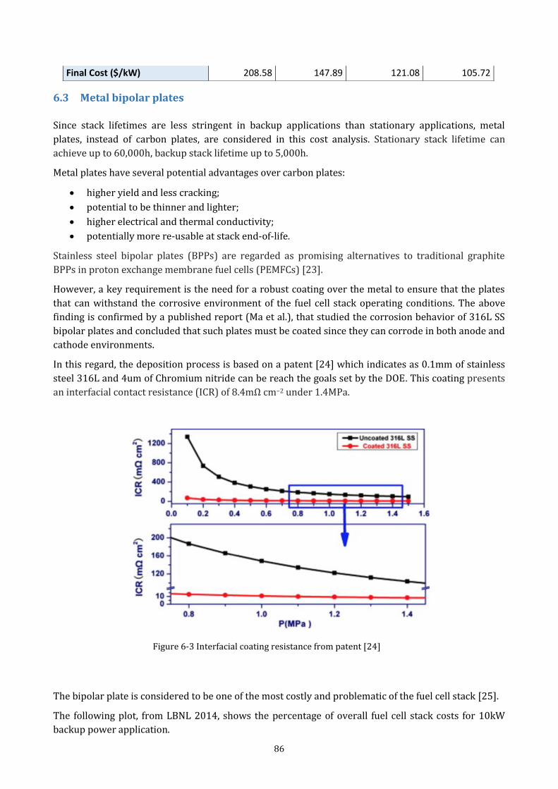
86
6.3 Metal bipolar plates
Since stack lifetimes are less stringent in backup applications than stationary applications, metal
plates, instead of carbon plates, are considered in this cost analysis. Stationary stack lifetime can
achieve up to 60,000h, backup stack lifetime up to 5,000h.
Metal plates have several potential advantages over carbon plates:
higher yield and less cracking;
potential to be thinner and lighter;
higher electrical and thermal conductivity;
potentially more re-usable at stack end-of-life.
Stainless steel bipolar plates (BPPs) are regarded as promising alternatives to traditional graphite
BPPs in proton exchange membrane fuel cells (PEMFCs) [23].
However, a key requirement is the need for a robust coating over the metal to ensure that the plates
that can withstand the corrosive environment of the fuel cell stack operating conditions. The above
finding is confirmed by a published report (Ma et al.), that studied the corrosion behavior of 316L SS
bipolar plates and concluded that such plates must be coated since they can corrode in both anode and
cathode environments.
In this regard, the deposition process is based on a patent [24] which indicates as 0.1mm of stainless
steel 316L and 4um of Chromium nitride can be reach the goals set by the DOE. This coating presents
an interfacial contact resistance (ICR) of 8.4mΩ cm−2 under 1.4MPa.
Figure 6-3 Interfacial coating resistance from patent [24]
The bipolar plate is considered to be one of the most costly and problematic of the fuel cell stack [25].
The following plot, from LBNL 2014, shows the percentage of overall fuel cell stack costs for 10kW
backup power application.
Final Cost ($/kW) 208.58 147.89 121.08 105.72
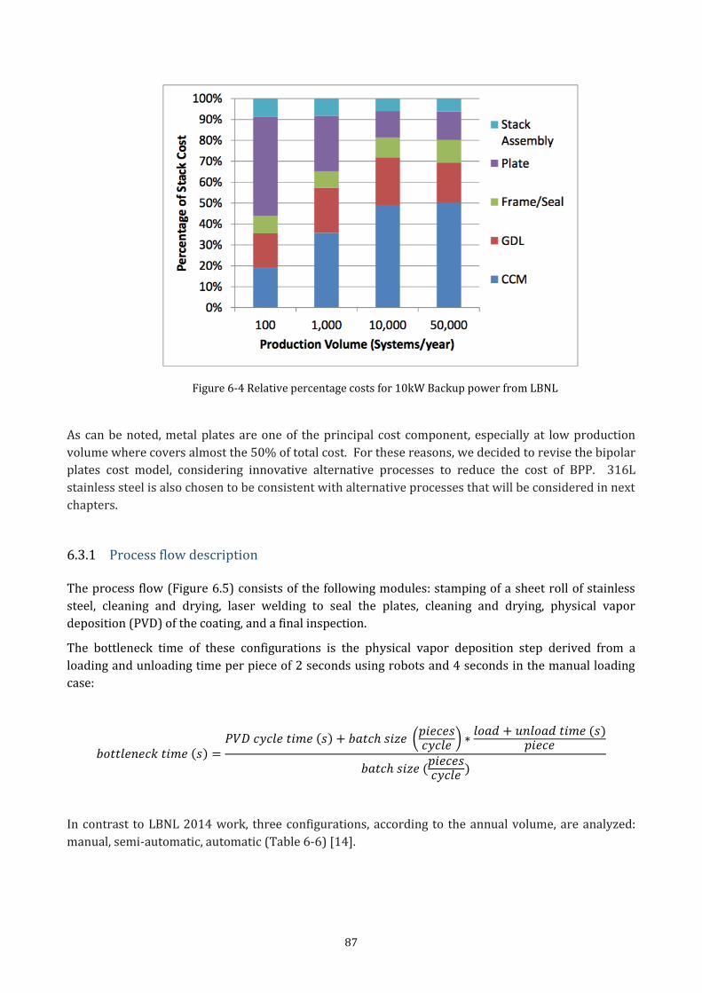
87
Figure 6-4 Relative percentage costs for 10kW Backup power from LBNL
As can be noted, metal plates are one of the principal cost component, especially at low production
volume where covers almost the 50% of total cost. For these reasons, we decided to revise the bipolar
plates cost model, considering innovative alternative processes to reduce the cost of BPP. 316L
stainless steel is also chosen to be consistent with alternative processes that will be considered in next
chapters.
6.3.1 Process flow description The process flow (Figure 6.5) consists of the following modules: stamping of a sheet roll of stainless
steel, cleaning and drying, laser welding to seal the plates, cleaning and drying, physical vapor
deposition (PVD) of the coating, and a final inspection.
The bottleneck time of these configurations is the physical vapor deposition step derived from a
loading and unloading time per piece of 2 seconds using robots and 4 seconds in the manual loading
case:
𝑏𝑜𝑡𝑡𝑙𝑒𝑛𝑒𝑐𝑘 𝑡𝑖𝑚𝑒 (𝑠) =𝑃𝑉𝐷 𝑐𝑦𝑐𝑙𝑒 𝑡𝑖𝑚𝑒 (𝑠) + 𝑏𝑎𝑡𝑐ℎ 𝑠𝑖𝑧𝑒 (
𝑝𝑖𝑒𝑐𝑒𝑠𝑐𝑦𝑐𝑙𝑒
) ∗𝑙𝑜𝑎𝑑 + 𝑢𝑛𝑙𝑜𝑎𝑑 𝑡𝑖𝑚𝑒 (𝑠)
𝑝𝑖𝑒𝑐𝑒
𝑏𝑎𝑡𝑐ℎ 𝑠𝑖𝑧𝑒 (𝑝𝑖𝑒𝑐𝑒𝑠𝑐𝑦𝑐𝑙𝑒
)
In contrast to LBNL 2014 work, three configurations, according to the annual volume, are analyzed:
manual, semi-automatic, automatic (Table 6-6) [14].
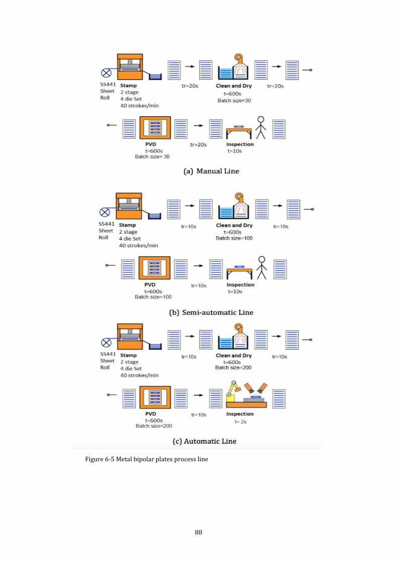
88
Figure 6-5 Metal bipolar plates process line
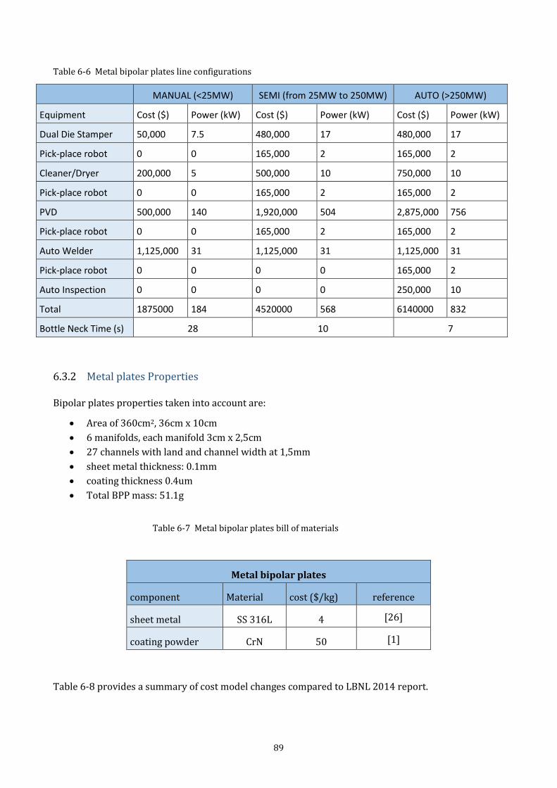
89
Table 6-6 Metal bipolar plates line configurations
MANUAL (<25MW) SEMI (from 25MW to 250MW) AUTO (>250MW)
Equipment Cost ($) Power (kW) Cost ($) Power (kW) Cost ($) Power (kW)
Dual Die Stamper 50,000 7.5 480,000 17 480,000 17
Pick-place robot 0 0 165,000 2 165,000 2
Cleaner/Dryer 200,000 5 500,000 10 750,000 10
Pick-place robot 0 0 165,000 2 165,000 2
PVD 500,000 140 1,920,000 504 2,875,000 756
Pick-place robot 0 0 165,000 2 165,000 2
Auto Welder 1,125,000 31 1,125,000 31 1,125,000 31
Pick-place robot 0 0 0 0 165,000 2
Auto Inspection 0 0 0 0 250,000 10
Total 1875000 184 4520000 568 6140000 832
Bottle Neck Time (s) 28 10 7
6.3.2 Metal plates Properties Bipolar plates properties taken into account are:
Area of 360cm2, 36cm x 10cm
6 manifolds, each manifold 3cm x 2,5cm
27 channels with land and channel width at 1,5mm
sheet metal thickness: 0.1mm
coating thickness 0.4um
Total BPP mass: 51.1g
Table 6-7 Metal bipolar plates bill of materials
Metal bipolar plates
component Material cost ($/kg) reference
sheet metal SS 316L 4 [26]
coating powder CrN 50 [1]
Table 6-8 provides a summary of cost model changes compared to LBNL 2014 report.
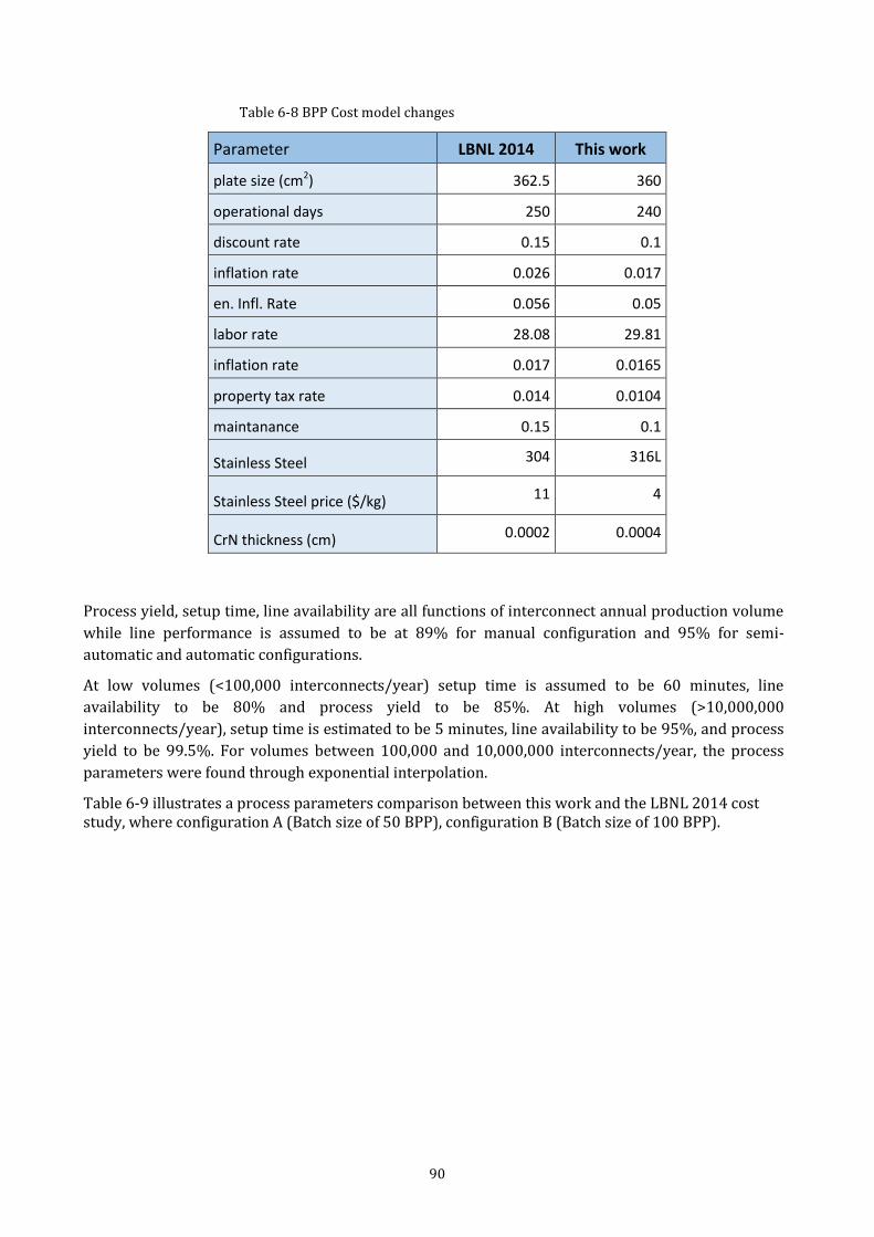
90
Table 6-8 BPP Cost model changes
Parameter LBNL 2014 This work
plate size (cm2) 362.5 360
operational days 250 240
discount rate 0.15 0.1
inflation rate 0.026 0.017
en. Infl. Rate 0.056 0.05
labor rate 28.08 29.81
inflation rate 0.017 0.0165
property tax rate 0.014 0.0104
maintanance 0.15 0.1
Stainless Steel 304 316L
Stainless Steel price ($/kg) 11 4
CrN thickness (cm) 0.0002 0.0004
Process yield, setup time, line availability are all functions of interconnect annual production volume
while line performance is assumed to be at 89% for manual configuration and 95% for semi-
automatic and automatic configurations.
At low volumes (<100,000 interconnects/year) setup time is assumed to be 60 minutes, line
availability to be 80% and process yield to be 85%. At high volumes (>10,000,000
interconnects/year), setup time is estimated to be 5 minutes, line availability to be 95%, and process
yield to be 99.5%. For volumes between 100,000 and 10,000,000 interconnects/year, the process
parameters were found through exponential interpolation.
Table 6-9 illustrates a process parameters comparison between this work and the LBNL 2014 cost study, where configuration A (Batch size of 50 BPP), configuration B (Batch size of 100 BPP).
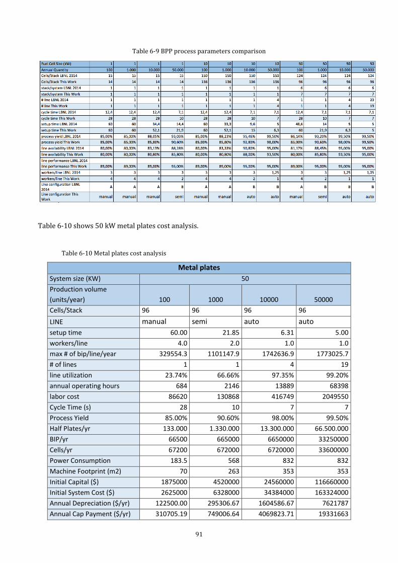
91
Table 6-9 BPP process parameters comparison
Table 6-10 shows 50 kW metal plates cost analysis.
Table 6-10 Metal plates cost analysis
Metal plates
System size (KW) 50
Production volume
(units/year) 100 1000 10000 50000
Cells/Stack 96 96 96 96
LINE manual semi auto auto
setup time 60.00 21.85 6.31 5.00
workers/line 4.0 2.0 1.0 1.0
max # of bip/line/year 329554.3 1101147.9 1742636.9 1773025.7
# of lines 1 1 4 19
line utilization 23.74% 66.66% 97.35% 99.20%
annual operating hours 684 2146 13889 68398
labor cost 86620 130868 416749 2049550
Cycle Time (s) 28 10 7 7
Process Yield 85.00% 90.60% 98.00% 99.50%
Half Plates/yr 133.000 1.330.000 13.300.000 66.500.000
BIP/yr 66500 665000 6650000 33250000
Cells/yr 67200 672000 6720000 33600000
Power Consumption 183.5 568 832 832
Machine Footprint (m2) 70 263 353 353
Initial Capital ($) 1875000 4520000 24560000 116660000
Initial System Cost ($) 2625000 6328000 34384000 163324000
Annual Depreciation ($/yr) 122500.00 295306.67 1604586.67 7621787
Annual Cap Payment ($/yr) 310705.19 749006.64 4069823.71 19331663
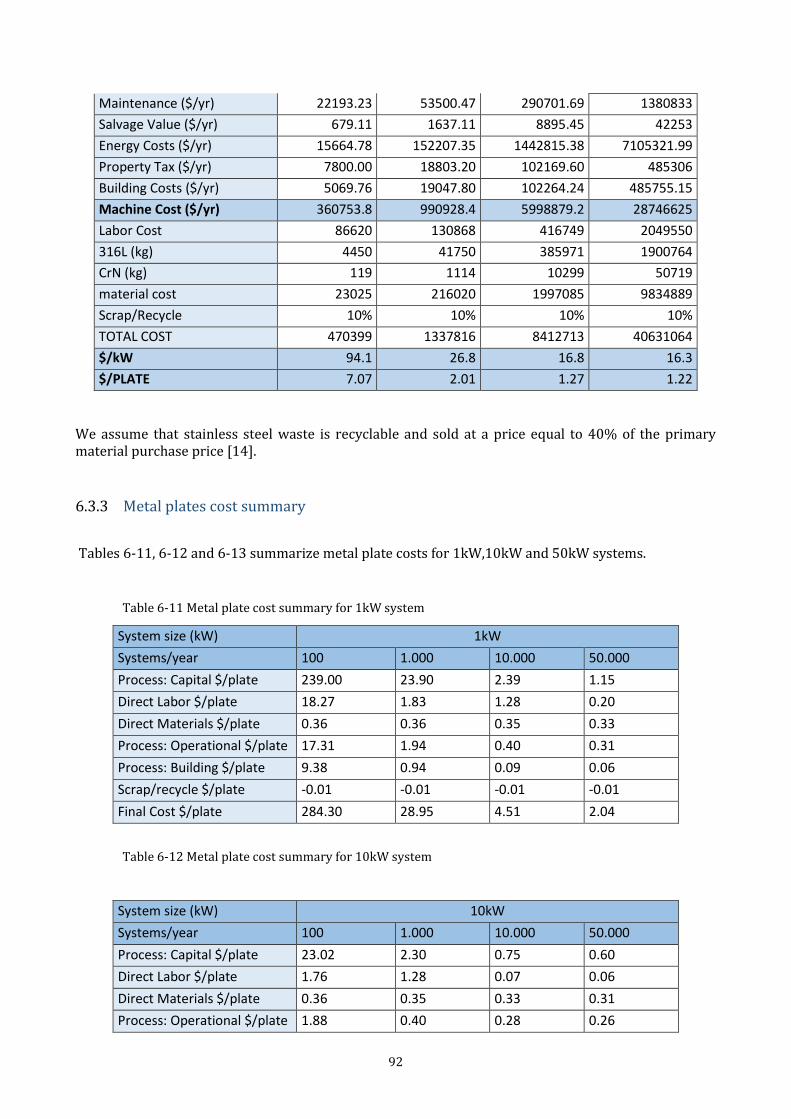
92
Maintenance ($/yr) 22193.23 53500.47 290701.69 1380833
Salvage Value ($/yr) 679.11 1637.11 8895.45 42253
Energy Costs ($/yr) 15664.78 152207.35 1442815.38 7105321.99
Property Tax ($/yr) 7800.00 18803.20 102169.60 485306
Building Costs ($/yr) 5069.76 19047.80 102264.24 485755.15
Machine Cost ($/yr) 360753.8 990928.4 5998879.2 28746625
Labor Cost 86620 130868 416749 2049550
316L (kg) 4450 41750 385971 1900764
CrN (kg) 119 1114 10299 50719
material cost 23025 216020 1997085 9834889
Scrap/Recycle 10% 10% 10% 10%
TOTAL COST 470399 1337816 8412713 40631064
$/kW 94.1 26.8 16.8 16.3
$/PLATE 7.07 2.01 1.27 1.22
We assume that stainless steel waste is recyclable and sold at a price equal to 40% of the primary material purchase price [14].
6.3.3 Metal plates cost summary
Tables 6-11, 6-12 and 6-13 summarize metal plate costs for 1kW,10kW and 50kW systems.
Table 6-11 Metal plate cost summary for 1kW system
System size (kW) 1kW
Systems/year 100 1.000 10.000 50.000
Process: Capital $/plate 239.00 23.90 2.39 1.15
Direct Labor $/plate 18.27 1.83 1.28 0.20
Direct Materials $/plate 0.36 0.36 0.35 0.33
Process: Operational $/plate 17.31 1.94 0.40 0.31
Process: Building $/plate 9.38 0.94 0.09 0.06
Scrap/recycle $/plate -0.01 -0.01 -0.01 -0.01
Final Cost $/plate 284.30 28.95 4.51 2.04
Table 6-12 Metal plate cost summary for 10kW system
System size (kW) 10kW
Systems/year 100 1.000 10.000 50.000
Process: Capital $/plate 23.02 2.30 0.75 0.60
Direct Labor $/plate 1.76 1.28 0.07 0.06
Direct Materials $/plate 0.36 0.35 0.33 0.31
Process: Operational $/plate 1.88 0.40 0.28 0.26
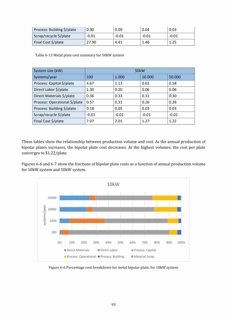
93
Process: Building $/plate 0.90 0.09 0.04 0.03
Scrap/recycle $/plate -0.01 -0.01 -0.01 -0.01
Final Cost $/plate 27.90 4.41 1.46 1.25
Table 6-13 Metal plate cost summary for 50kW system
System size (kW) 50kW
Systems/year 100 1.000 10.000 50.000
Process: Capital $/plate 4.67 1.13 0.61 0.58
Direct Labor $/plate 1.30 0.20 0.06 0.06
Direct Materials $/plate 0.36 0.33 0.31 0.30
Process: Operational $/plate 0.57 0.31 0.26 0.26
Process: Building $/plate 0.18 0.05 0.03 0.03
Scrap/recycle $/plate -0.01 -0.01 -0.01 -0.01
Final Cost $/plate 7.07 2.01 1.27 1.22
These tables show the relationship between production volume and cost. As the annual production of
bipolar plates increases, the bipolar plate cost decreases. At the highest volumes, the cost per plate
converges to $1.22/plate.
Figures 6-6 and 6-7 show the fractions of bipolar plate costs as a function of annual production volume
for 10kW system and 50kW system.
Figure 6-6 Percentage cost breakdown for metal bipolar plate, for 10kW system
0% 10% 20% 30% 40% 50% 60% 70% 80% 90% 100%
100
1000
10000
50000
syst
ems/
year
10kW
Direct Materials Direct Labor Process: Capital
Process: Operational Process: Building Material Scrap
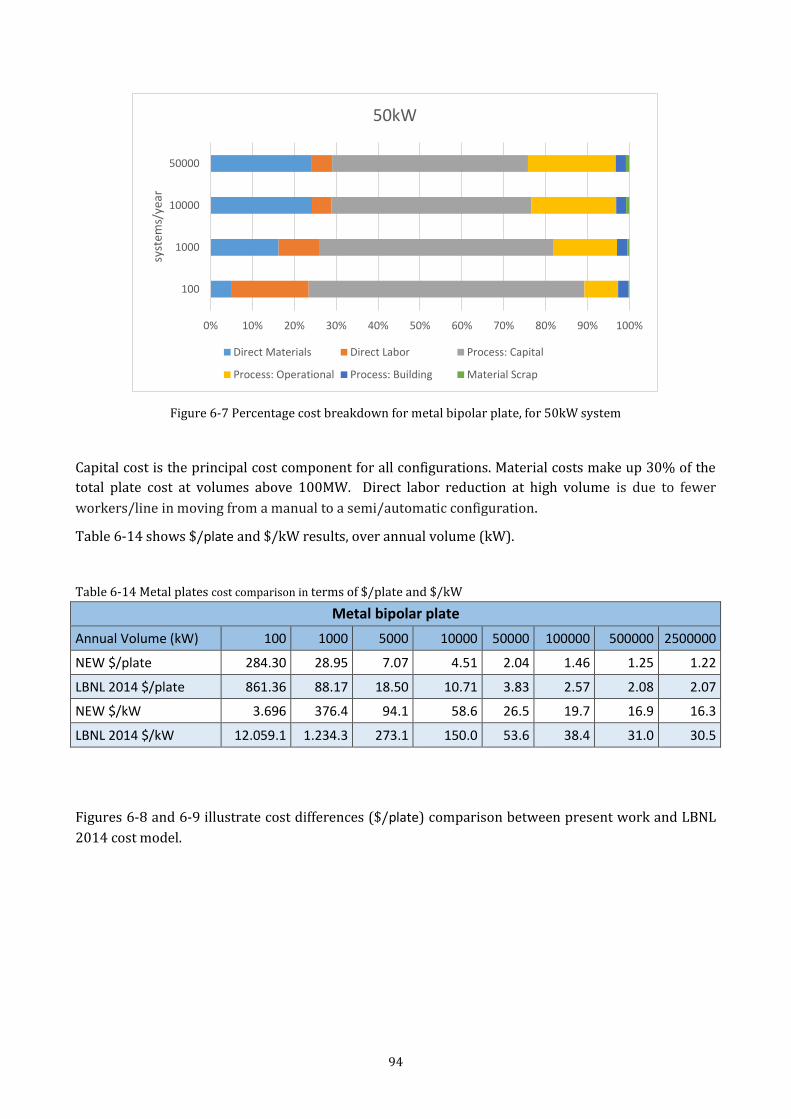
94
Figure 6-7 Percentage cost breakdown for metal bipolar plate, for 50kW system
Capital cost is the principal cost component for all configurations. Material costs make up 30% of the
total plate cost at volumes above 100MW. Direct labor reduction at high volume is due to fewer
workers/line in moving from a manual to a semi/automatic configuration.
Table 6-14 shows $/plate and $/kW results, over annual volume (kW).
Table 6-14 Metal plates cost comparison in terms of $/plate and $/kW
Metal bipolar plate
Annual Volume (kW) 100 1000 5000 10000 50000 100000 500000 2500000
NEW $/plate 284.30 28.95 7.07 4.51 2.04 1.46 1.25 1.22
LBNL 2014 $/plate 861.36 88.17 18.50 10.71 3.83 2.57 2.08 2.07
NEW $/kW 3.696 376.4 94.1 58.6 26.5 19.7 16.9 16.3
LBNL 2014 $/kW 12.059.1 1.234.3 273.1 150.0 53.6 38.4 31.0 30.5
Figures 6-8 and 6-9 illustrate cost differences ($/plate) comparison between present work and LBNL
2014 cost model.
0% 10% 20% 30% 40% 50% 60% 70% 80% 90% 100%
100
1000
10000
50000sy
stem
s/ye
ar
50kW
Direct Materials Direct Labor Process: Capital
Process: Operational Process: Building Material Scrap
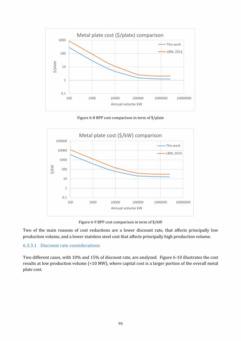
95
Figure 6-8 BPP cost comparison in term of $/plate
Figure 6-9 BPP cost comparison in term of $/kW
Two of the main reasons of cost reductions are a lower discount rate, that affects principally low
production volume, and a lower stainless steel cost that affects principally high production volume.
6.3.3.1 Discount rate considerations
Two different cases, with 10% and 15% of discount rate, are analyzed. Figure 6-10 illustrates the cost
results at low production volume (<10 MW), where capital cost is a larger portion of the overall metal
plate cost.
0.1
1
10
100
1000
100 1000 10000 100000 1000000 10000000
$/p
late
Annual volume kW
Metal plate cost ($/plate) comparison
This work
LBNL 2014
0.1
1
10
100
1000
10000
100000
100 1000 10000 100000 1000000 10000000
$/k
W
Annual volume kW
Metal plate cost ($/kW) comparison
This work
LBNL 2014
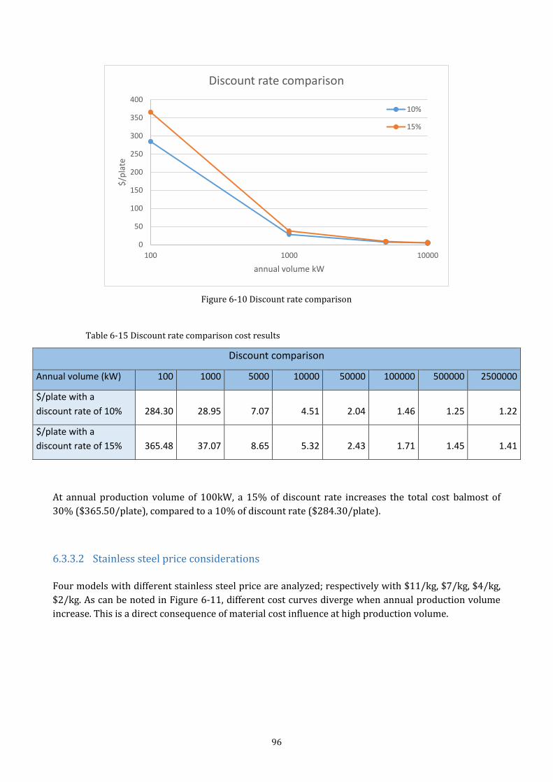
96
Figure 6-10 Discount rate comparison
Table 6-15 Discount rate comparison cost results
Discount comparison
Annual volume (kW) 100 1000 5000 10000 50000 100000 500000 2500000
$/plate with a
discount rate of 10% 284.30 28.95 7.07 4.51 2.04 1.46 1.25 1.22
$/plate with a
discount rate of 15% 365.48 37.07 8.65 5.32 2.43 1.71 1.45 1.41
At annual production volume of 100kW, a 15% of discount rate increases the total cost balmost of
30% ($365.50/plate), compared to a 10% of discount rate ($284.30/plate).
6.3.3.2 Stainless steel price considerations
Four models with different stainless steel price are analyzed; respectively with $11/kg, $7/kg, $4/kg,
$2/kg. As can be noted in Figure 6-11, different cost curves diverge when annual production volume
increase. This is a direct consequence of material cost influence at high production volume.
0
50
100
150
200
250
300
350
400
100 1000 10000
$/p
late
annual volume kW
Discount rate comparison
10%
15%
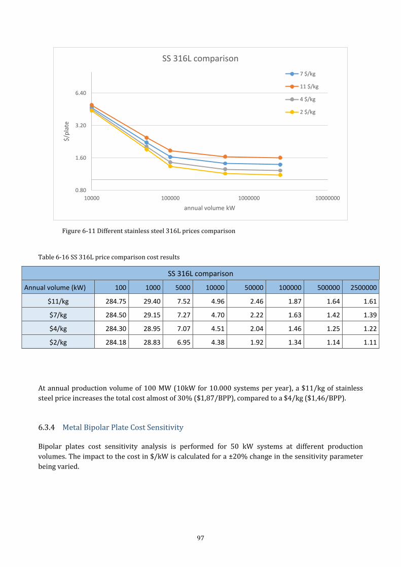
97
Figure 6-11 Different stainless steel 316L prices comparison
Table 6-16 SS 316L price comparison cost results
SS 316L comparison
Annual volume (kW) 100 1000 5000 10000 50000 100000 500000 2500000
$11/kg 284.75 29.40 7.52 4.96 2.46 1.87 1.64 1.61
$7/kg 284.50 29.15 7.27 4.70 2.22 1.63 1.42 1.39
$4/kg 284.30 28.95 7.07 4.51 2.04 1.46 1.25 1.22
$2/kg 284.18 28.83 6.95 4.38 1.92 1.34 1.14 1.11
At annual production volume of 100 MW (10kW for 10.000 systems per year), a $11/kg of stainless
steel price increases the total cost almost of 30% ($1,87/BPP), compared to a $4/kg ($1,46/BPP).
6.3.4 Metal Bipolar Plate Cost Sensitivity Bipolar plates cost sensitivity analysis is performed for 50 kW systems at different production
volumes. The impact to the cost in $/kW is calculated for a ±20% change in the sensitivity parameter
being varied.
0.80
1.60
3.20
6.40
10000 100000 1000000 10000000
$/p
late
annual volume kW
SS 316L comparison
7 $/kg
11 $/kg
4 $/kg
2 $/kg
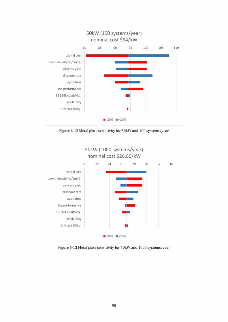
98
Figure 6-12 Metal plate sensitivity for 50kW and 100 systems/year
Figure 6-13 Metal plate sensitivity for 50kW and 1000 systems/year
80 85 90 95 100 105 110
capital cost
power density W/cm^2]
process yield
discount rate
cycle time
line performance
SS 316L cost($/kg)
availability
CrN cost ($/kg)
50kW (100 systems/year) nominal cost $94/kW
-20% +20%
20 22 24 26 28 30 32 34
capital cost
power density W/cm^2]
process yield
discount rate
cycle time
line performance
SS 316L cost($/kg)
availability
CrN cost ($/kg)
50kW (1000 systems/year) nominal cost $26.80/kW
-20% +20%
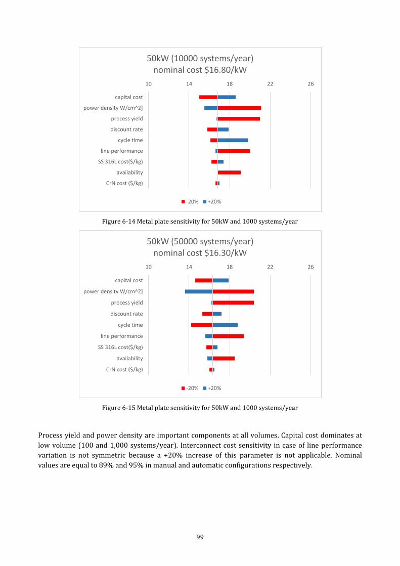
99
Figure 6-14 Metal plate sensitivity for 50kW and 1000 systems/year
Figure 6-15 Metal plate sensitivity for 50kW and 1000 systems/year
Process yield and power density are important components at all volumes. Capital cost dominates at
low volume (100 and 1,000 systems/year). Interconnect cost sensitivity in case of line performance
variation is not symmetric because a +20% increase of this parameter is not applicable. Nominal
values are equal to 89% and 95% in manual and automatic configurations respectively.
10 14 18 22 26
capital cost
power density W/cm^2]
process yield
discount rate
cycle time
line performance
SS 316L cost($/kg)
availability
CrN cost ($/kg)
50kW (10000 systems/year) nominal cost $16.80/kW
-20% +20%
10 14 18 22 26
capital cost
power density W/cm^2]
process yield
discount rate
cycle time
line performance
SS 316L cost($/kg)
availability
CrN cost ($/kg)
50kW (50000 systems/year) nominal cost $16.30/kW
-20% +20%
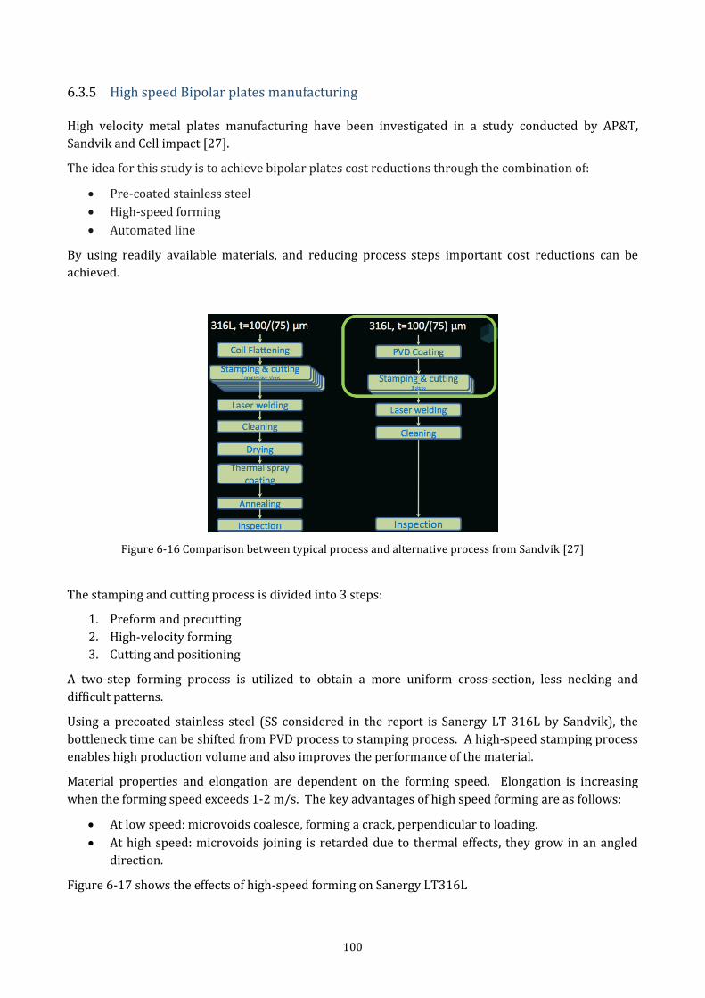
100
6.3.5 High speed Bipolar plates manufacturing High velocity metal plates manufacturing have been investigated in a study conducted by AP&T,
Sandvik and Cell impact [27].
The idea for this study is to achieve bipolar plates cost reductions through the combination of:
Pre-coated stainless steel
High-speed forming
Automated line
By using readily available materials, and reducing process steps important cost reductions can be
achieved.
Figure 6-16 Comparison between typical process and alternative process from Sandvik [27]
The stamping and cutting process is divided into 3 steps:
1. Preform and precutting
2. High-velocity forming
3. Cutting and positioning
A two-step forming process is utilized to obtain a more uniform cross-section, less necking and
difficult patterns.
Using a precoated stainless steel (SS considered in the report is Sanergy LT 316L by Sandvik), the
bottleneck time can be shifted from PVD process to stamping process. A high-speed stamping process
enables high production volume and also improves the performance of the material.
Material properties and elongation are dependent on the forming speed. Elongation is increasing
when the forming speed exceeds 1-2 m/s. The key advantages of high speed forming are as follows:
At low speed: microvoids coalesce, forming a crack, perpendicular to loading.
At high speed: microvoids joining is retarded due to thermal effects, they grow in an angled
direction.
Figure 6-17 shows the effects of high-speed forming on Sanergy LT316L
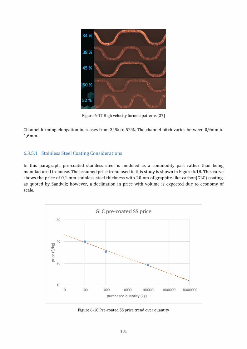
101
Figure 6-17 High velocity formed patterns [27]
Channel forming elongation increases from 34% to 52%. The channel pitch varies between 0,9mm to
1,6mm.
6.3.5.1 Stainless Steel Coating Considerations
In this paragraph, pre-coated stainless steel is modeled as a commodity part rather than being
manufactured in-house. The assumed price trend used in this study is shown in Figure 6.18. This curve
shows the price of 0,1 mm stainless steel thickness with 20 nm of graphite-like-carbon(GLC) coating,
as quoted by Sandvik; however, a declination in price with volume is expected due to economy of
scale.
Figure 6-18 Pre-coated SS price trend over quantity
10
20
40
80
10 100 1000 10000 100000 1000000 10000000
pri
ce (
$/k
g)
purchased quantity (kg)
GLC pre-coated SS price
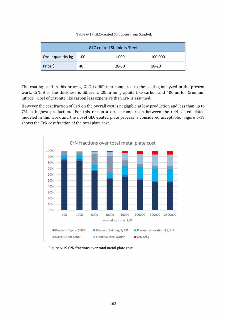
102
Table 6-17 GLC-coated SS quotes from Sandvik
GLC coated Stainless Steel
Order quantity kg 100 1.000 100.000
Price $ 40 28-30 18-20
The coating used in this process, GLC, is different compared to the coating analyzed in the present
work, CrN. Also the thickness is different, 20nm for graphite like carbon and 400nm for Cromium
nitride. Cost of graphite like carbon less expensive than CrN is assumed.
However the cost fraction of CrN on the overall cost is negligible at low production and less than up to
7% at highest production. For this reason a direct comparison between the CrN-coated plated
modeled in this work and the novel GLC-coated plate process is considered acceptable. Figure 6-19
shows the CrN cost fraction of the total plate cost.
Figure 6-19 CrN fractions over total metal plate cost
0%
10%
20%
30%
40%
50%
60%
70%
80%
90%
100%
100 1000 5000 10000 50000 100000 500000 2500000
annual volume kW
CrN fractions over total metal plate cost
Process: Capital $/BIP Process: Building $/BIP Process: Operational $/BIP
Direct Labor $/BIP stainless steel $/BPP CrN $/kg
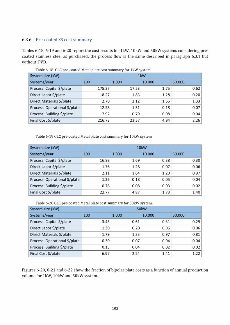
103
6.3.6 Pre-coated SS cost summary Tables 6-18, 6-19 and 6-20 report the cost results for 1kW, 10kW and 50kW systems considering pre-
coated stainless steel as purchased; the process flow is the same described in paragraph 6.3.1 but
without PVD.
Table 6-18 GLC pre-coated Metal plate cost summary for 1kW system
System size (kW) 1kW
Systems/year 100 1.000 10.000 50.000
Process: Capital $/plate 175.27 17.53 1.75 0.62
Direct Labor $/plate 18.27 1.83 1.28 0.20
Direct Materials $/plate 2.70 2.12 1.65 1.33
Process: Operational $/plate 12.58 1.31 0.18 0.07
Process: Building $/plate 7.92 0.79 0.08 0.04
Final Cost $/plate 216.73 23.57 4.94 2.26
Table 6-19 GLC pre-coated Metal plate cost summary for 10kW system
System size (kW) 10kW
Systems/year 100 1.000 10.000 50.000
Process: Capital $/plate 16.88 1.69 0.38 0.30
Direct Labor $/plate 1.76 1.28 0.07 0.06
Direct Materials $/plate 2.11 1.64 1.20 0.97
Process: Operational $/plate 1.26 0.18 0.05 0.04
Process: Building $/plate 0.76 0.08 0.03 0.02
Final Cost $/plate 22.77 4.87 1.73 1.40
Table 6-20 GLC pre-coated Metal plate cost summary for 50kW system.
System size (kW) 50kW
Systems/year 100 1.000 10.000 50.000
Process: Capital $/plate 3.43 0.61 0.31 0.29
Direct Labor $/plate 1.30 0.20 0.06 0.06
Direct Materials $/plate 1.79 1.33 0.97 0.81
Process: Operational $/plate 0.30 0.07 0.04 0.04
Process: Building $/plate 0.15 0.04 0.02 0.02
Final Cost $/plate 6.97 2.24 1.41 1.22
Figures 6-20, 6-21 and 6-22 show the fraction of bipolar plate costs as a function of annual production
volume for 1kW, 10kW and 50kW system.
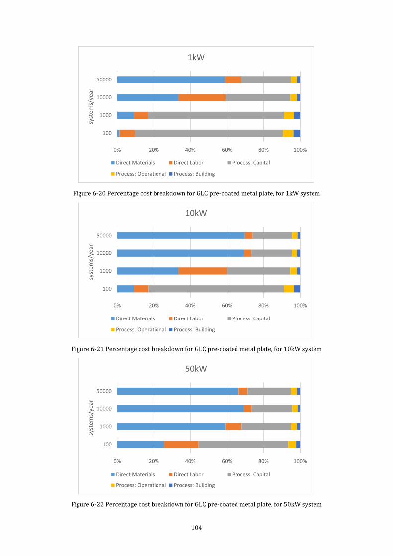
104
Figure 6-20 Percentage cost breakdown for GLC pre-coated metal plate, for 1kW system
Figure 6-21 Percentage cost breakdown for GLC pre-coated metal plate, for 10kW system
Figure 6-22 Percentage cost breakdown for GLC pre-coated metal plate, for 50kW system
0% 20% 40% 60% 80% 100%
100
1000
10000
50000
syst
ems/
year
1kW
Direct Materials Direct Labor Process: Capital
Process: Operational Process: Building
0% 20% 40% 60% 80% 100%
100
1000
10000
50000
syst
ems/
year
10kW
Direct Materials Direct Labor Process: Capital
Process: Operational Process: Building
0% 20% 40% 60% 80% 100%
100
1000
10000
50000
syst
ems/
year
50kW
Direct Materials Direct Labor Process: Capital
Process: Operational Process: Building
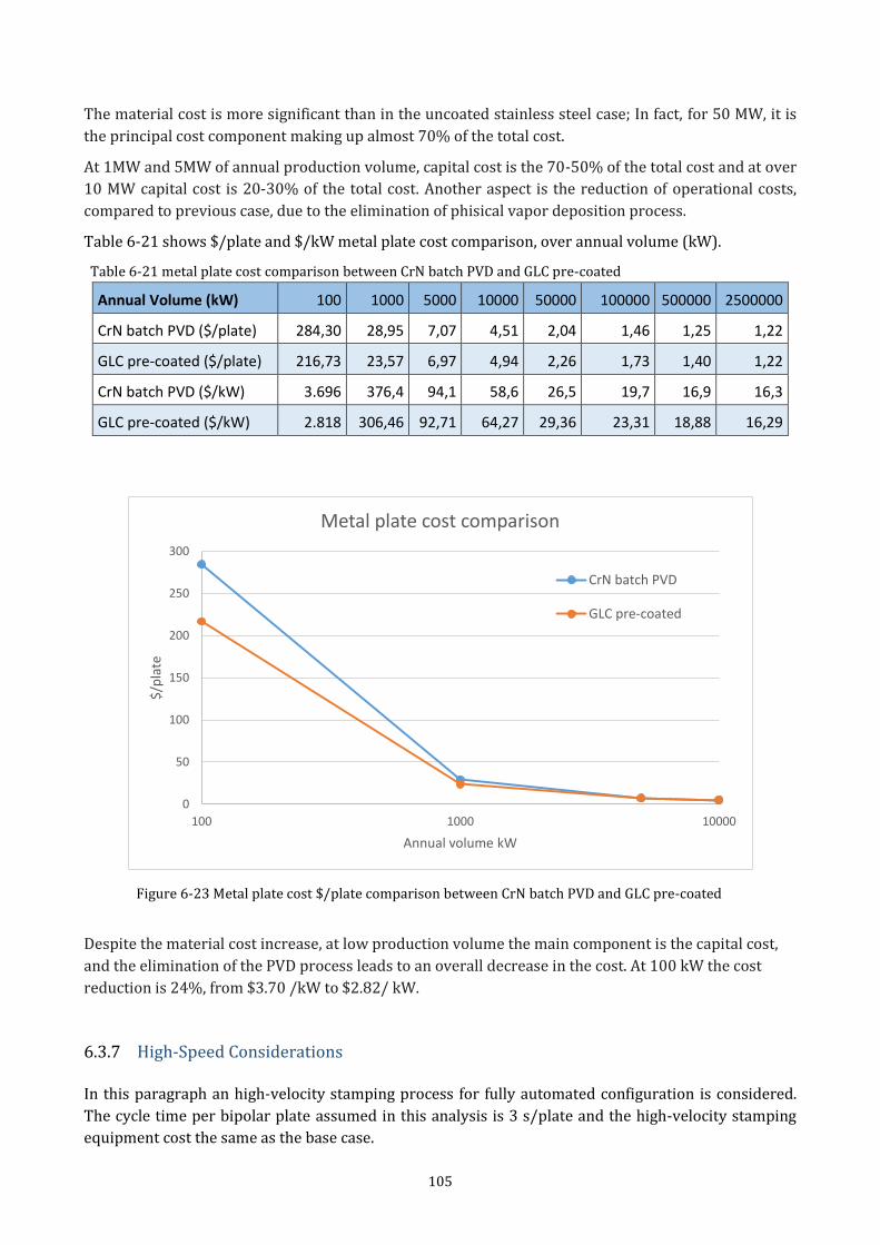
105
The material cost is more significant than in the uncoated stainless steel case; In fact, for 50 MW, it is
the principal cost component making up almost 70% of the total cost.
At 1MW and 5MW of annual production volume, capital cost is the 70-50% of the total cost and at over
10 MW capital cost is 20-30% of the total cost. Another aspect is the reduction of operational costs,
compared to previous case, due to the elimination of phisical vapor deposition process.
Table 6-21 shows $/plate and $/kW metal plate cost comparison, over annual volume (kW).
Table 6-21 metal plate cost comparison between CrN batch PVD and GLC pre-coated
Annual Volume (kW) 100 1000 5000 10000 50000 100000 500000 2500000
CrN batch PVD ($/plate) 284,30 28,95 7,07 4,51 2,04 1,46 1,25 1,22
GLC pre-coated ($/plate) 216,73 23,57 6,97 4,94 2,26 1,73 1,40 1,22
CrN batch PVD ($/kW) 3.696 376,4 94,1 58,6 26,5 19,7 16,9 16,3
GLC pre-coated ($/kW) 2.818 306,46 92,71 64,27 29,36 23,31 18,88 16,29
Figure 6-23 Metal plate cost $/plate comparison between CrN batch PVD and GLC pre-coated
Despite the material cost increase, at low production volume the main component is the capital cost,
and the elimination of the PVD process leads to an overall decrease in the cost. At 100 kW the cost
reduction is 24%, from $3.70 /kW to $2.82/ kW.
6.3.7 High-Speed Considerations In this paragraph an high-velocity stamping process for fully automated configuration is considered.
The cycle time per bipolar plate assumed in this analysis is 3 s/plate and the high-velocity stamping
equipment cost the same as the base case.
0
50
100
150
200
250
300
100 1000 10000
$/p
late
Annual volume kW
Metal plate cost comparison
CrN batch PVD
GLC pre-coated
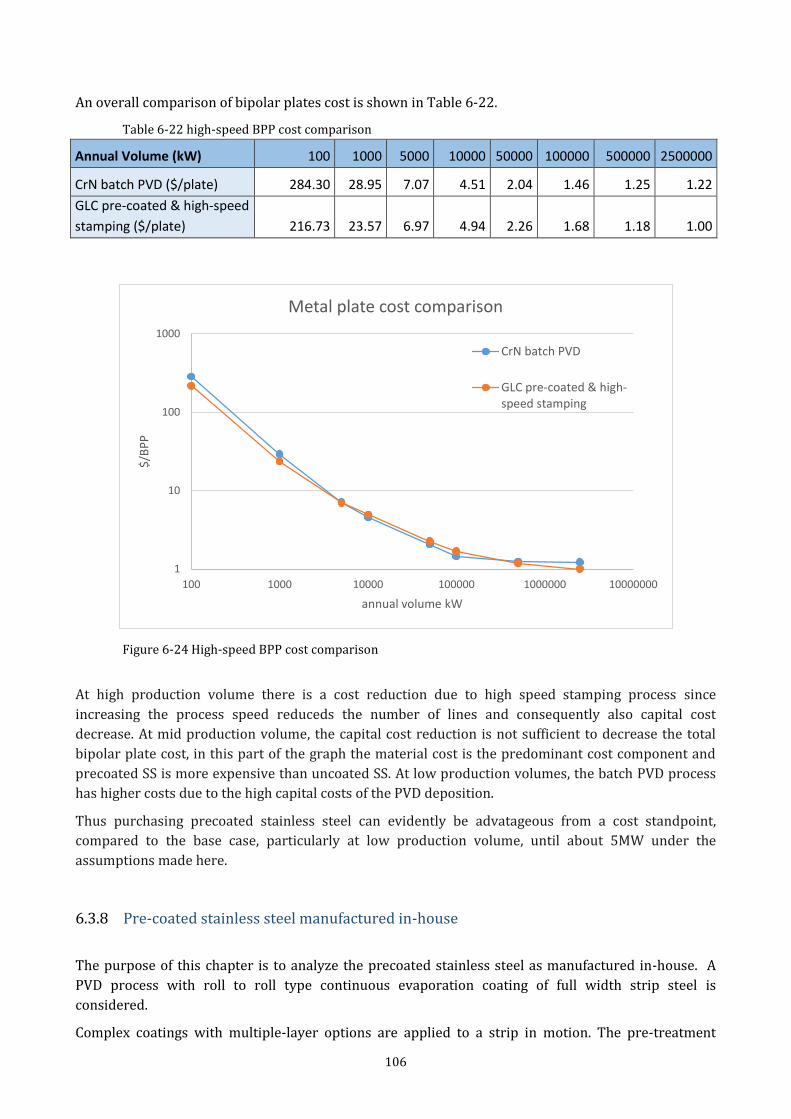
106
An overall comparison of bipolar plates cost is shown in Table 6-22.
Table 6-22 high-speed BPP cost comparison
Annual Volume (kW) 100 1000 5000 10000 50000 100000 500000 2500000
CrN batch PVD ($/plate) 284.30 28.95 7.07 4.51 2.04 1.46 1.25 1.22
GLC pre-coated & high-speed
stamping ($/plate) 216.73 23.57 6.97 4.94 2.26 1.68 1.18 1.00
Figure 6-24 High-speed BPP cost comparison
At high production volume there is a cost reduction due to high speed stamping process since
increasing the process speed reduceds the number of lines and consequently also capital cost
decrease. At mid production volume, the capital cost reduction is not sufficient to decrease the total
bipolar plate cost, in this part of the graph the material cost is the predominant cost component and
precoated SS is more expensive than uncoated SS. At low production volumes, the batch PVD process
has higher costs due to the high capital costs of the PVD deposition.
Thus purchasing precoated stainless steel can evidently be advatageous from a cost standpoint,
compared to the base case, particularly at low production volume, until about 5MW under the
assumptions made here.
6.3.8 Pre-coated stainless steel manufactured in-house
The purpose of this chapter is to analyze the precoated stainless steel as manufactured in-house. A
PVD process with roll to roll type continuous evaporation coating of full width strip steel is
considered.
Complex coatings with multiple-layer options are applied to a strip in motion. The pre-treatment
1
10
100
1000
100 1000 10000 100000 1000000 10000000
$/B
PP
annual volume kW
Metal plate cost comparison
CrN batch PVD
GLC pre-coated & high-speed stamping
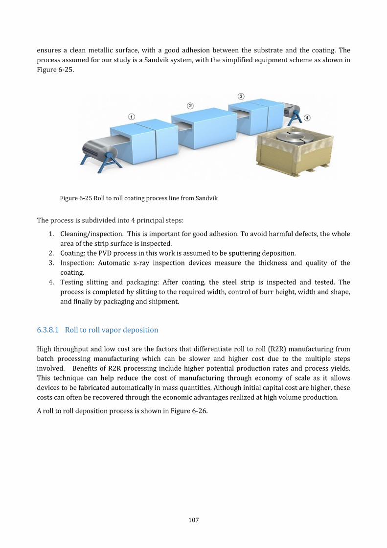
107
ensures a clean metallic surface, with a good adhesion between the substrate and the coating. The
process assumed for our study is a Sandvik system, with the simplified equipment scheme as shown in
Figure 6-25.
Figure 6-25 Roll to roll coating process line from Sandvik
The process is subdivided into 4 principal steps:
1. Cleaning/inspection. This is important for good adhesion. To avoid harmful defects, the whole
area of the strip surface is inspected.
2. Coating: the PVD process in this work is assumed to be sputtering deposition.
3. Inspection: Automatic x-ray inspection devices measure the thickness and quality of the
coating.
4. Testing slitting and packaging: After coating, the steel strip is inspected and tested. The
process is completed by slitting to the required width, control of burr height, width and shape,
and finally by packaging and shipment.
6.3.8.1 Roll to roll vapor deposition
High throughput and low cost are the factors that differentiate roll to roll (R2R) manufacturing from
batch processing manufacturing which can be slower and higher cost due to the multiple steps
involved. Benefits of R2R processing include higher potential production rates and process yields.
This technique can help reduce the cost of manufacturing through economy of scale as it allows
devices to be fabricated automatically in mass quantities. Although initial capital cost are higher, these
costs can often be recovered through the economic advantages realized at high volume production.
A roll to roll deposition process is shown in Figure 6-26.
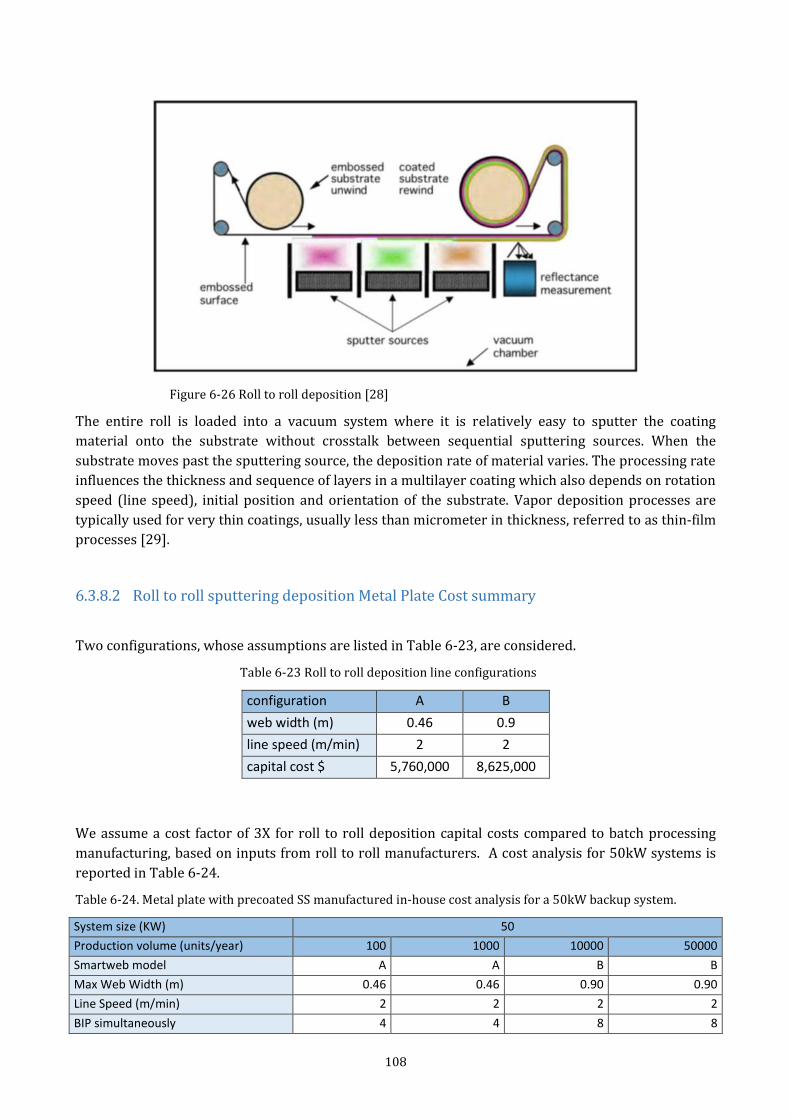
108
Figure 6-26 Roll to roll deposition [28]
The entire roll is loaded into a vacuum system where it is relatively easy to sputter the coating
material onto the substrate without crosstalk between sequential sputtering sources. When the
substrate moves past the sputtering source, the deposition rate of material varies. The processing rate
influences the thickness and sequence of layers in a multilayer coating which also depends on rotation
speed (line speed), initial position and orientation of the substrate. Vapor deposition processes are
typically used for very thin coatings, usually less than micrometer in thickness, referred to as thin-film
processes [29].
6.3.8.2 Roll to roll sputtering deposition Metal Plate Cost summary
Two configurations, whose assumptions are listed in Table 6-23, are considered.
Table 6-23 Roll to roll deposition line configurations
configuration A B
web width (m) 0.46 0.9
line speed (m/min) 2 2
capital cost $ 5,760,000 8,625,000
We assume a cost factor of 3X for roll to roll deposition capital costs compared to batch processing
manufacturing, based on inputs from roll to roll manufacturers. A cost analysis for 50kW systems is
reported in Table 6-24.
Table 6-24. Metal plate with precoated SS manufactured in-house cost analysis for a 50kW backup system.
System size (KW) 50
Production volume (units/year) 100 1000 10000 50000
Smartweb model A A B B
Max Web Width (m) 0.46 0.46 0.90 0.90
Line Speed (m/min) 2 2 2 2
BIP simultaneously 4 4 8 8
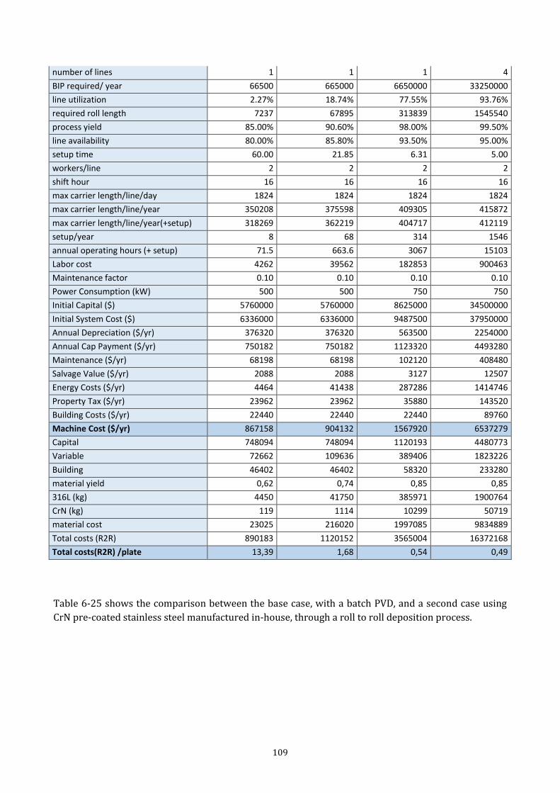
109
number of lines 1 1 1 4
BIP required/ year 66500 665000 6650000 33250000
line utilization 2.27% 18.74% 77.55% 93.76%
required roll length 7237 67895 313839 1545540
process yield 85.00% 90.60% 98.00% 99.50%
line availability 80.00% 85.80% 93.50% 95.00%
setup time 60.00 21.85 6.31 5.00
workers/line 2 2 2 2
shift hour 16 16 16 16
max carrier length/line/day 1824 1824 1824 1824
max carrier length/line/year 350208 375598 409305 415872
max carrier length/line/year(+setup) 318269 362219 404717 412119
setup/year 8 68 314 1546
annual operating hours (+ setup) 71.5 663.6 3067 15103
Labor cost 4262 39562 182853 900463
Maintenance factor 0.10 0.10 0.10 0.10
Power Consumption (kW) 500 500 750 750
Initial Capital ($) 5760000 5760000 8625000 34500000
Initial System Cost ($) 6336000 6336000 9487500 37950000
Annual Depreciation ($/yr) 376320 376320 563500 2254000
Annual Cap Payment ($/yr) 750182 750182 1123320 4493280
Maintenance ($/yr) 68198 68198 102120 408480
Salvage Value ($/yr) 2088 2088 3127 12507
Energy Costs ($/yr) 4464 41438 287286 1414746
Property Tax ($/yr) 23962 23962 35880 143520
Building Costs ($/yr) 22440 22440 22440 89760
Machine Cost ($/yr) 867158 904132 1567920 6537279
Capital 748094 748094 1120193 4480773
Variable 72662 109636 389406 1823226
Building 46402 46402 58320 233280
material yield 0,62 0,74 0,85 0,85
316L (kg) 4450 41750 385971 1900764
CrN (kg) 119 1114 10299 50719
material cost 23025 216020 1997085 9834889
Total costs (R2R) 890183 1120152 3565004 16372168
Total costs(R2R) /plate 13,39 1,68 0,54 0,49
Table 6-25 shows the comparison between the base case, with a batch PVD, and a second case using
CrN pre-coated stainless steel manufactured in-house, through a roll to roll deposition process.
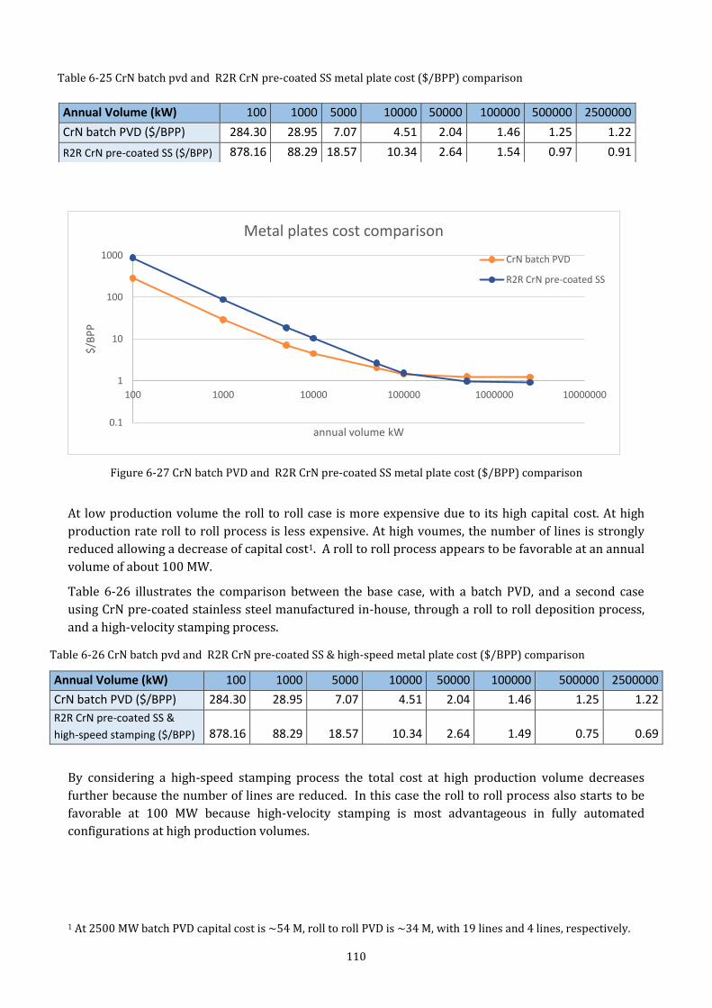
110
Figure 6-27 CrN batch PVD and R2R CrN pre-coated SS metal plate cost ($/BPP) comparison
At low production volume the roll to roll case is more expensive due to its high capital cost. At high
production rate roll to roll process is less expensive. At high voumes, the number of lines is strongly
reduced allowing a decrease of capital cost1. A roll to roll process appears to be favorable at an annual
volume of about 100 MW.
Table 6-26 illustrates the comparison between the base case, with a batch PVD, and a second case
using CrN pre-coated stainless steel manufactured in-house, through a roll to roll deposition process,
and a high-velocity stamping process.
Annual Volume (kW) 100 1000 5000 10000 50000 100000 500000 2500000
CrN batch PVD ($/BPP) 284.30 28.95 7.07 4.51 2.04 1.46 1.25 1.22
R2R CrN pre-coated SS &
high-speed stamping ($/BPP) 878.16 88.29 18.57 10.34 2.64 1.49 0.75 0.69
By considering a high-speed stamping process the total cost at high production volume decreases
further because the number of lines are reduced. In this case the roll to roll process also starts to be
favorable at 100 MW because high-velocity stamping is most advantageous in fully automated
configurations at high production volumes.
1 At 2500 MW batch PVD capital cost is ~54 M, roll to roll PVD is ~34 M, with 19 lines and 4 lines, respectively.
0.1
1
10
100
1000
100 1000 10000 100000 1000000 10000000
$/B
PP
annual volume kW
Metal plates cost comparison
CrN batch PVD
R2R CrN pre-coated SS
Table 6-25 CrN batch pvd and R2R CrN pre-coated SS metal plate cost ($/BPP) comparison
Annual Volume (kW) 100 1000 5000 10000 50000 100000 500000 2500000
CrN batch PVD ($/BPP) 284.30 28.95 7.07 4.51 2.04 1.46 1.25 1.22
R2R CrN pre-coated SS ($/BPP) 878.16 88.29 18.57 10.34 2.64 1.54 0.97 0.91
Table 6-26 CrN batch pvd and R2R CrN pre-coated SS & high-speed metal plate cost ($/BPP) comparison
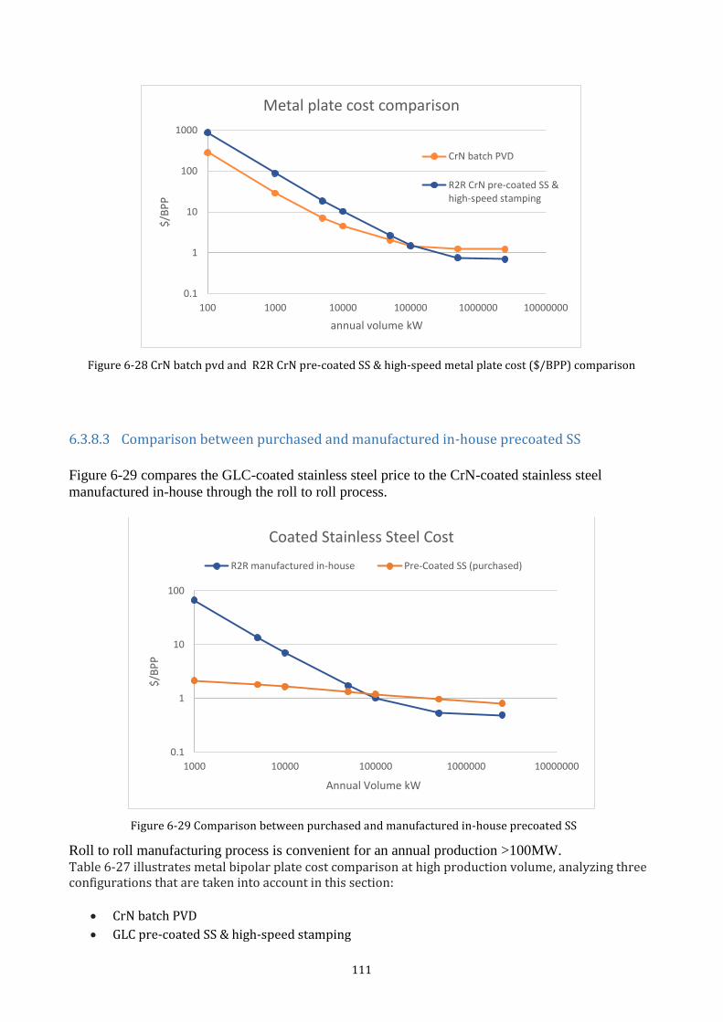
111
Figure 6-28 CrN batch pvd and R2R CrN pre-coated SS & high-speed metal plate cost ($/BPP) comparison
6.3.8.3 Comparison between purchased and manufactured in-house precoated SS
Figure 6-29 compares the GLC-coated stainless steel price to the CrN-coated stainless steel
manufactured in-house through the roll to roll process.
Figure 6-29 Comparison between purchased and manufactured in-house precoated SS
Roll to roll manufacturing process is convenient for an annual production >100MW. Table 6-27 illustrates metal bipolar plate cost comparison at high production volume, analyzing three configurations that are taken into account in this section:
CrN batch PVD
GLC pre-coated SS & high-speed stamping
0.1
1
10
100
1000
100 1000 10000 100000 1000000 10000000
$/B
PP
annual volume kW
Metal plate cost comparison
CrN batch PVD
R2R CrN pre-coated SS &high-speed stamping
0.1
1
10
100
1000 10000 100000 1000000 10000000
$/B
PP
Annual Volume kW
Coated Stainless Steel Cost
R2R manufactured in-house Pre-Coated SS (purchased)
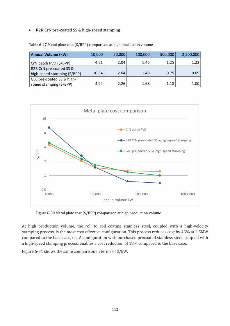
112
R2R CrN pre-coated SS & high-speed stamping
Annual Volume (kW) 10,000 50,000 100,000 500,000 2,500,000
CrN batch PVD ($/BPP) 4.51 2.04 1.46 1.25 1.22
R2R CrN pre-coated SS & high-speed stamping ($/BPP) 10.34 2.64 1.49 0.75 0.69
GLC pre-coated SS & high-speed stamping ($/BPP) 4.94 2.26 1.68 1.18 1.00
Figure 6-30 Metal plate cost ($/BPP) comparison at high production volume
At high production volume, the roll to roll coating stainless steel, coupled with a high-velocity
stamping process, is the most cost effective configuration. This process reduces cost by 43% at 2.5MW
compared to the base case, of. A configuration with purchased precoated stainless steel, coupled with
a high-speed stamping process, enables a cost reduction of 18% compared to the base case.
Figure 6-31 shows the same comparison in terms of $/kW.
0.5
1
2
4
8
16
10000 100000 1000000 10000000
$/B
PP
annual volume kW
Metal plate cost comparison
CrN batch PVD
R2R CrN pre-coated SS & high-speed stamping
GLC pre-coated SS & high-speed stamping
Table 6-27 Metal plate cost ($/BPP) comparison at high production volume
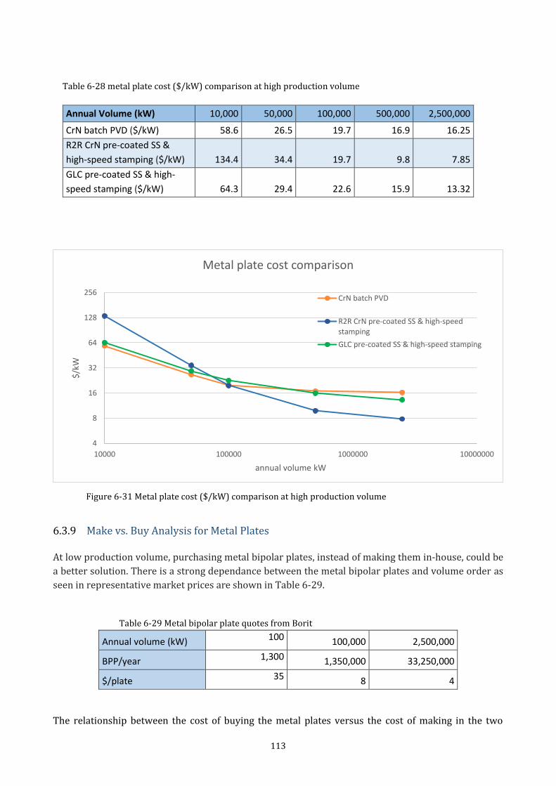
113
Figure 6-31 Metal plate cost ($/kW) comparison at high production volume
6.3.9 Make vs. Buy Analysis for Metal Plates At low production volume, purchasing metal bipolar plates, instead of making them in-house, could be
a better solution. There is a strong dependance between the metal bipolar plates and volume order as
seen in representative market prices are shown in Table 6-29.
Table 6-29 Metal bipolar plate quotes from Borit
Annual volume (kW) 100 100,000 2,500,000
BPP/year 1,300 1,350,000 33,250,000
$/plate 35 8 4
The relationship between the cost of buying the metal plates versus the cost of making in the two
4
8
16
32
64
128
256
10000 100000 1000000 10000000
$/k
W
annual volume kW
Metal plate cost comparison
CrN batch PVD
R2R CrN pre-coated SS & high-speedstamping
GLC pre-coated SS & high-speed stamping
Table 6-28 metal plate cost ($/kW) comparison at high production volume
Annual Volume (kW) 10,000 50,000 100,000 500,000 2,500,000
CrN batch PVD ($/kW) 58.6 26.5 19.7 16.9 16.25
R2R CrN pre-coated SS &
high-speed stamping ($/kW) 134.4 34.4 19.7 9.8 7.85
GLC pre-coated SS & high-
speed stamping ($/kW) 64.3 29.4 22.6 15.9 13.32
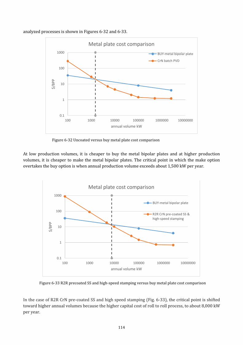
114
analyzed processes is shown in Figures 6-32 and 6-33.
Figure 6-32 Uncoated versus buy metal plate cost comparison
At low production volumes, it is cheaper to buy the metal bipolar plates and at higher production
volumes, it is cheaper to make the metal bipolar plates. The critical point in which the make option
overtakes the buy option is when annual production volume exceeds about 1,500 kW per year.
Figure 6-33 R2R precoated SS and high-speed stamping versus buy metal plate cost comparison
In the case of R2R CrN pre-coated SS and high speed stamping (Fig. 6-33), the critical point is shifted
toward higher annual volumes because the higher capital cost of roll to roll process, to about 8,000 kW
per year.
0.1
1
10
100
1000
100 1000 10000 100000 1000000 10000000
$/B
PP
annual volume kW
Metal plate cost comparison
BUY-metal bipolar plate
CrN batch PVD
0.1
1
10
100
1000
100 1000 10000 100000 1000000 10000000
$/B
PP
annual volume kW
Metal plate cost comparison
BUY-metal bipolar plate
R2R CrN pre-coated SS &high-speed stamping
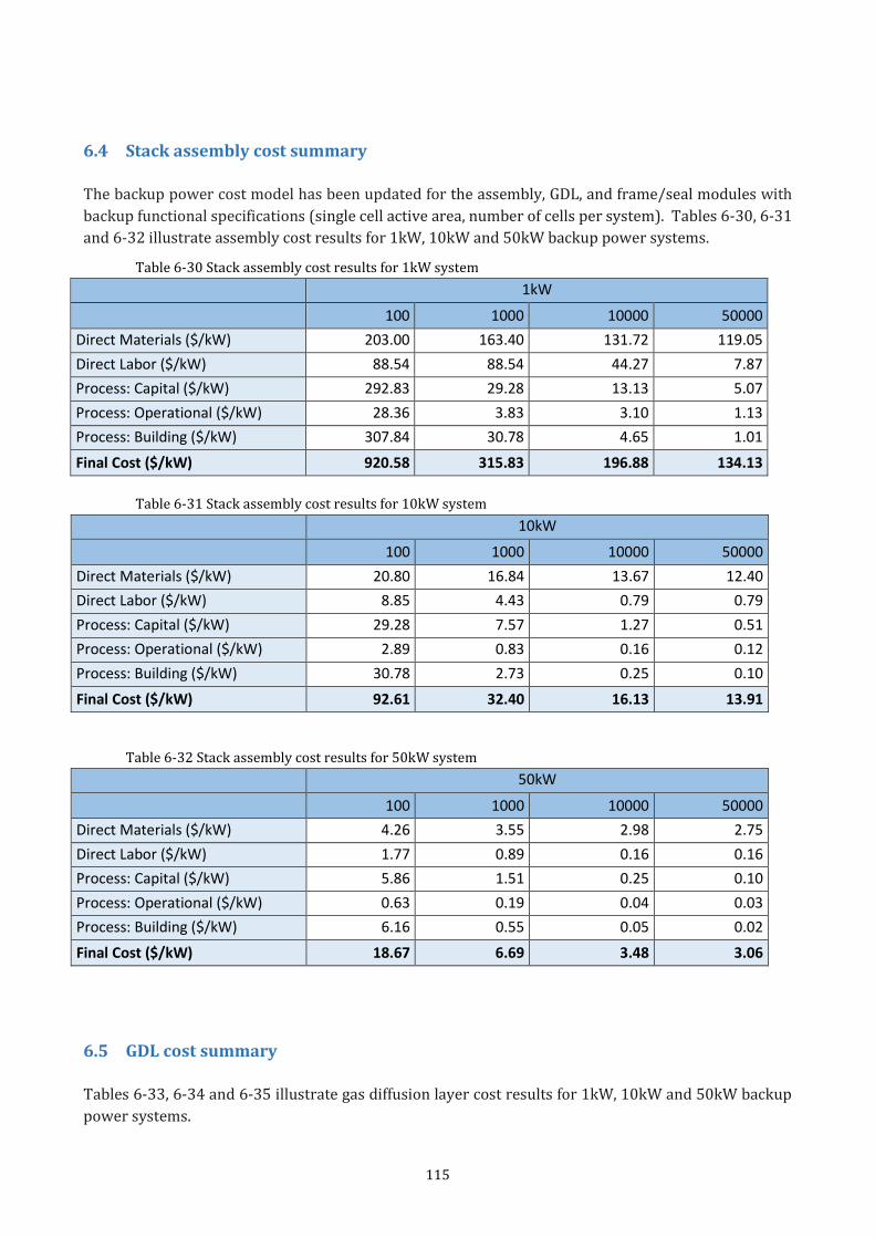
115
6.4 Stack assembly cost summary
The backup power cost model has been updated for the assembly, GDL, and frame/seal modules with
backup functional specifications (single cell active area, number of cells per system). Tables 6-30, 6-31
and 6-32 illustrate assembly cost results for 1kW, 10kW and 50kW backup power systems.
Table 6-30 Stack assembly cost results for 1kW system
1kW
100 1000 10000 50000
Direct Materials ($/kW) 203.00 163.40 131.72 119.05
Direct Labor ($/kW) 88.54 88.54 44.27 7.87
Process: Capital ($/kW) 292.83 29.28 13.13 5.07
Process: Operational ($/kW) 28.36 3.83 3.10 1.13
Process: Building ($/kW) 307.84 30.78 4.65 1.01
Final Cost ($/kW) 920.58 315.83 196.88 134.13
Table 6-31 Stack assembly cost results for 10kW system
10kW
100 1000 10000 50000
Direct Materials ($/kW) 20.80 16.84 13.67 12.40
Direct Labor ($/kW) 8.85 4.43 0.79 0.79
Process: Capital ($/kW) 29.28 7.57 1.27 0.51
Process: Operational ($/kW) 2.89 0.83 0.16 0.12
Process: Building ($/kW) 30.78 2.73 0.25 0.10
Final Cost ($/kW) 92.61 32.40 16.13 13.91
Table 6-32 Stack assembly cost results for 50kW system
50kW
100 1000 10000 50000
Direct Materials ($/kW) 4.26 3.55 2.98 2.75
Direct Labor ($/kW) 1.77 0.89 0.16 0.16
Process: Capital ($/kW) 5.86 1.51 0.25 0.10
Process: Operational ($/kW) 0.63 0.19 0.04 0.03
Process: Building ($/kW) 6.16 0.55 0.05 0.02
Final Cost ($/kW) 18.67 6.69 3.48 3.06
6.5 GDL cost summary
Tables 6-33, 6-34 and 6-35 illustrate gas diffusion layer cost results for 1kW, 10kW and 50kW backup
power systems.
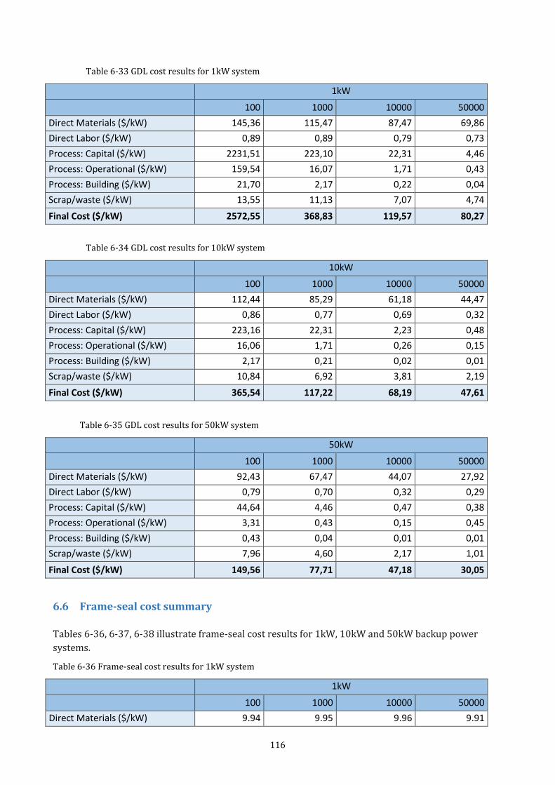
116
Table 6-33 GDL cost results for 1kW system
1kW
100 1000 10000 50000
Direct Materials ($/kW) 145,36 115,47 87,47 69,86
Direct Labor ($/kW) 0,89 0,89 0,79 0,73
Process: Capital ($/kW) 2231,51 223,10 22,31 4,46
Process: Operational ($/kW) 159,54 16,07 1,71 0,43
Process: Building ($/kW) 21,70 2,17 0,22 0,04
Scrap/waste ($/kW) 13,55 11,13 7,07 4,74
Final Cost ($/kW) 2572,55 368,83 119,57 80,27
Table 6-34 GDL cost results for 10kW system
10kW
100 1000 10000 50000
Direct Materials ($/kW) 112,44 85,29 61,18 44,47
Direct Labor ($/kW) 0,86 0,77 0,69 0,32
Process: Capital ($/kW) 223,16 22,31 2,23 0,48
Process: Operational ($/kW) 16,06 1,71 0,26 0,15
Process: Building ($/kW) 2,17 0,21 0,02 0,01
Scrap/waste ($/kW) 10,84 6,92 3,81 2,19
Final Cost ($/kW) 365,54 117,22 68,19 47,61
Table 6-35 GDL cost results for 50kW system
50kW
100 1000 10000 50000
Direct Materials ($/kW) 92,43 67,47 44,07 27,92
Direct Labor ($/kW) 0,79 0,70 0,32 0,29
Process: Capital ($/kW) 44,64 4,46 0,47 0,38
Process: Operational ($/kW) 3,31 0,43 0,15 0,45
Process: Building ($/kW) 0,43 0,04 0,01 0,01
Scrap/waste ($/kW) 7,96 4,60 2,17 1,01
Final Cost ($/kW) 149,56 77,71 47,18 30,05
6.6 Frame-seal cost summary
Tables 6-36, 6-37, 6-38 illustrate frame-seal cost results for 1kW, 10kW and 50kW backup power
systems.
Table 6-36 Frame-seal cost results for 1kW system
1kW
100 1000 10000 50000
Direct Materials ($/kW) 9.94 9.95 9.96 9.91
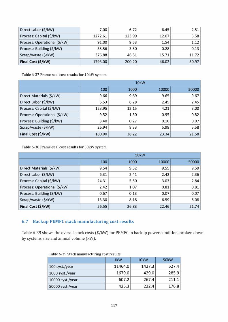
117
Direct Labor ($/kW) 7.00 6.72 6.45 2.51
Process: Capital ($/kW) 1272.61 123.99 12.07 5.58
Process: Operational ($/kW) 91.00 9.53 1.54 1.12
Process: Building ($/kW) 35.56 3.50 0.28 0.13
Scrap/waste ($/kW) 376.88 46.51 15.71 11.72
Final Cost ($/kW) 1793.00 200.20 46.02 30.97
Table 6-37 Frame-seal cost results for 10kW system
10kW
100 1000 10000 50000
Direct Materials ($/kW) 9.66 9.69 9.65 9.67
Direct Labor ($/kW) 6.53 6.28 2.45 2.45
Process: Capital ($/kW) 123.95 12.15 4.21 3.00
Process: Operational ($/kW) 9.52 1.50 0.95 0.82
Process: Building ($/kW) 3.40 0.27 0.10 0.07
Scrap/waste ($/kW) 26.94 8.33 5.98 5.58
Final Cost ($/kW) 180.00 38.22 23.34 21.58
Table 6-38 Frame-seal cost results for 50kW system
50kW
100 1000 10000 50000
Direct Materials ($/kW) 9.54 9.52 9.55 9.59
Direct Labor ($/kW) 6.31 2.41 2.42 2.36
Process: Capital ($/kW) 24.31 5.50 3.03 2.84
Process: Operational ($/kW) 2.42 1.07 0.81 0.81
Process: Building ($/kW) 0.67 0.13 0.07 0.07
Scrap/waste ($/kW) 13.30 8.18 6.59 6.08
Final Cost ($/kW) 56.55 26.83 22.46 21.74
6.7 Backup PEMFC stack manufacturing cost results
Table 6-39 shows the overall stack costs ($/kW) for PEMFC in backup power condition, broken down
by systems size and annual volume (kW).
Table 6-39 Stack manufacturing cost results
1kW 10kW 50kW
100 syst./year 11464.0 1427.3 527.4
1000 syst./year 1679.0 429.0 285.9
10000 syst./year 607.2 267.4 211.1
50000 syst./year 425.3 222.4 176.8
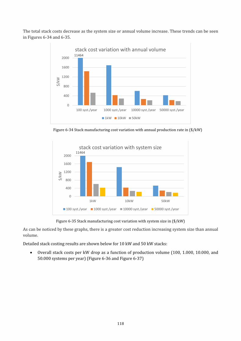
118
The total stack costs decrease as the system size or annual volume increase. These trends can be seen
in Figures 6-34 and 6-35.
Figure 6-34 Stack manufacturing cost variation with annual production rate in ($/kW)
Figure 6-35 Stack manufacturing cost variation with system size in ($/kW)
As can be noticed by these graphs, there is a greater cost reduction increasing system size than annual
volume.
Detailed stack costing results are shown below for 10 kW and 50 kW stacks:
Overall stack costs per kW drop as a function of production volume (100, 1.000, 10.000, and
50.000 systems per year) (Figure 6-36 and Figure 6-37)
11464
0
400
800
1200
1600
2000
100 syst./year 1000 syst./year 10000 syst./year 50000 syst./year
$/k
W
stack cost variation with annual volume
1kW 10kW 50kW
11464
0
400
800
1200
1600
2000
1kW 10kW 50kW
$/k
W
stack cost variation with system size
100 syst./year 1000 syst./year 10000 syst./year 50000 syst./year
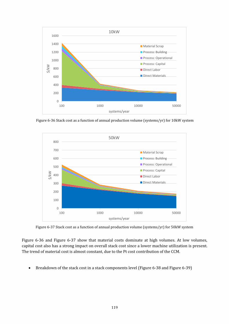
119
Figure 6-36 Stack cost as a function of annual production volume (systems/yr) for 10kW system
Figure 6-37 Stack cost as a function of annual production volume (systems/yr) for 50kW system
Figure 6-36 and Figure 6-37 show that material costs dominate at high volumes. At low volumes,
capital cost also has a strong impact on overall stack cost since a lower machine utilization is present.
The trend of material cost is almost constant, due to the Pt cost contribution of the CCM.
Breakdown of the stack cost in a stack components level (Figure 6-38 and Figure 6-39)
0
200
400
600
800
1000
1200
1400
1600
100 1000 10000 50000
$/k
W
systems/year
10kW
Material Scrap
Process: Building
Process: Operational
Process: Capital
Direct Labor
Direct Materials
0
100
200
300
400
500
600
700
800
100 1000 10000 50000
$/k
W
systems/year
50kW
Material Scrap
Process: Building
Process: Operational
Process: Capital
Direct Labor
Direct Materials
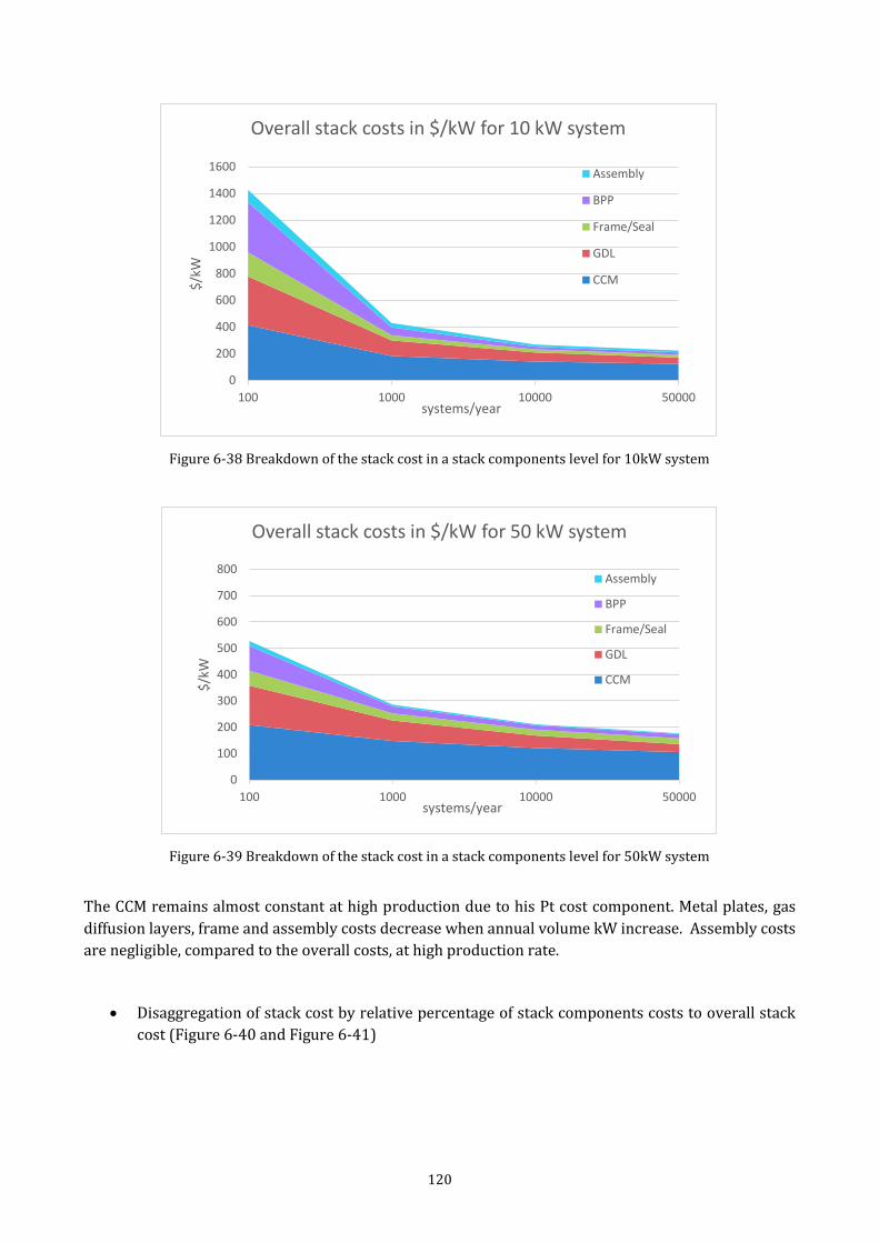
120
Figure 6-38 Breakdown of the stack cost in a stack components level for 10kW system
Figure 6-39 Breakdown of the stack cost in a stack components level for 50kW system
The CCM remains almost constant at high production due to his Pt cost component. Metal plates, gas
diffusion layers, frame and assembly costs decrease when annual volume kW increase. Assembly costs
are negligible, compared to the overall costs, at high production rate.
Disaggregation of stack cost by relative percentage of stack components costs to overall stack
cost (Figure 6-40 and Figure 6-41)
0
200
400
600
800
1000
1200
1400
1600
100 1000 10000 50000
$/k
W
systems/year
Overall stack costs in $/kW for 10 kW system
Assembly
BPP
Frame/Seal
GDL
CCM
0
100
200
300
400
500
600
700
800
100 1000 10000 50000
$/k
W
systems/year
Overall stack costs in $/kW for 50 kW system
Assembly
BPP
Frame/Seal
GDL
CCM
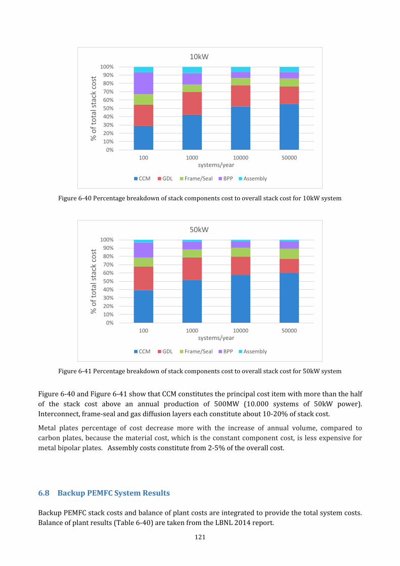
121
Figure 6-40 Percentage breakdown of stack components cost to overall stack cost for 10kW system
Figure 6-41 Percentage breakdown of stack components cost to overall stack cost for 50kW system
Figure 6-40 and Figure 6-41 show that CCM constitutes the principal cost item with more than the half
of the stack cost above an annual production of 500MW (10.000 systems of 50kW power).
Interconnect, frame-seal and gas diffusion layers each constitute about 10-20% of stack cost.
Metal plates percentage of cost decrease more with the increase of annual volume, compared to
carbon plates, because the material cost, which is the constant component cost, is less expensive for
metal bipolar plates. Assembly costs constitute from 2-5% of the overall cost.
6.8 Backup PEMFC System Results
Backup PEMFC stack costs and balance of plant costs are integrated to provide the total system costs.
Balance of plant results (Table 6-40) are taken from the LBNL 2014 report.
0%
10%
20%
30%
40%
50%
60%
70%
80%
90%
100%
100 1000 10000 50000
% o
f to
tal s
tack
co
st
systems/year
10kW
CCM GDL Frame/Seal BPP Assembly
0%
10%
20%
30%
40%
50%
60%
70%
80%
90%
100%
100 1000 10000 50000
% o
f to
tal s
tack
co
st
systems/year
50kW
CCM GDL Frame/Seal BPP Assembly
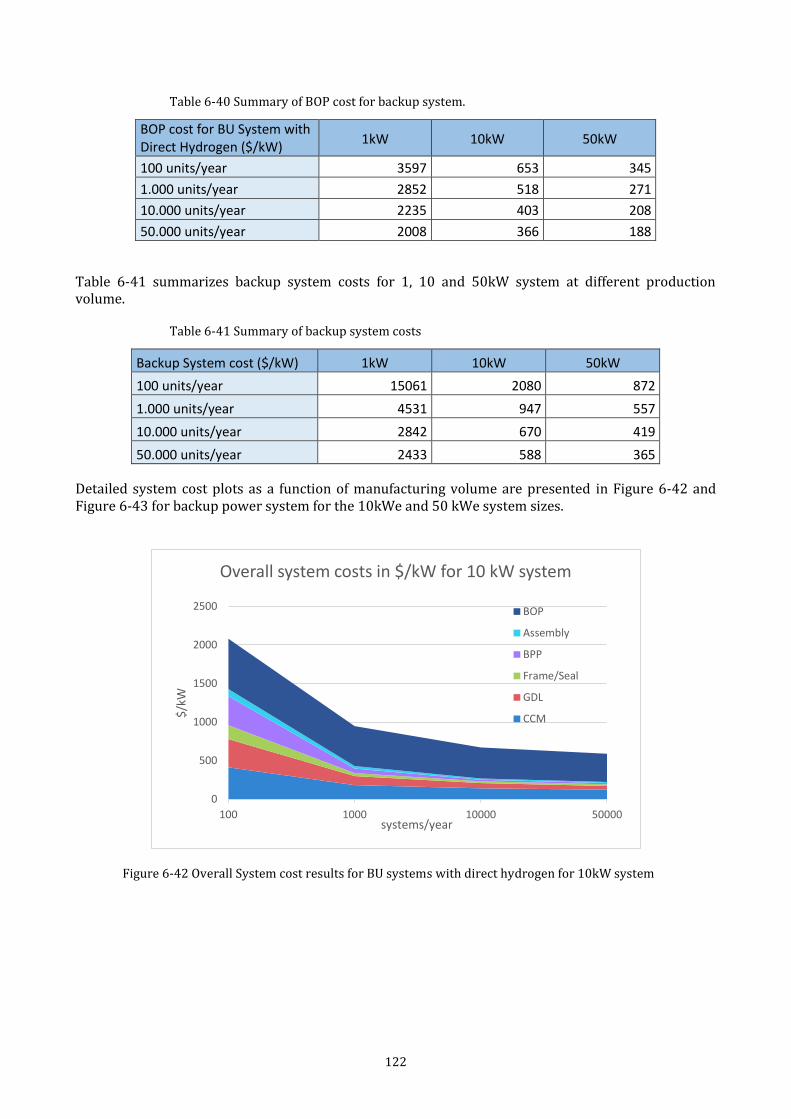
122
Table 6-40 Summary of BOP cost for backup system.
BOP cost for BU System with Direct Hydrogen ($/kW)
1kW 10kW 50kW
100 units/year 3597 653 345
1.000 units/year 2852 518 271
10.000 units/year 2235 403 208
50.000 units/year 2008 366 188
Table 6-41 summarizes backup system costs for 1, 10 and 50kW system at different production volume.
Table 6-41 Summary of backup system costs
Backup System cost ($/kW) 1kW 10kW 50kW
100 units/year 15061 2080 872
1.000 units/year 4531 947 557
10.000 units/year 2842 670 419
50.000 units/year 2433 588 365
Detailed system cost plots as a function of manufacturing volume are presented in Figure 6-42 and Figure 6-43 for backup power system for the 10kWe and 50 kWe system sizes.
Figure 6-42 Overall System cost results for BU systems with direct hydrogen for 10kW system
0
500
1000
1500
2000
2500
100 1000 10000 50000
$/k
W
systems/year
Overall system costs in $/kW for 10 kW system
BOP
Assembly
BPP
Frame/Seal
GDL
CCM
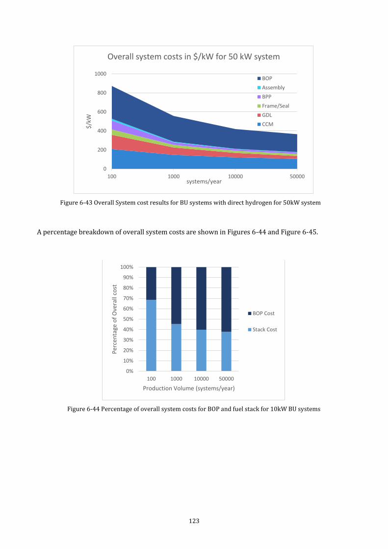
123
Figure 6-43 Overall System cost results for BU systems with direct hydrogen for 50kW system
A percentage breakdown of overall system costs are shown in Figures 6-44 and Figure 6-45.
Figure 6-44 Percentage of overall system costs for BOP and fuel stack for 10kW BU systems
0
200
400
600
800
1000
100 1000 10000 50000
$/k
W
systems/year
Overall system costs in $/kW for 50 kW system
BOP
Assembly
BPP
Frame/Seal
GDL
CCM
0%
10%
20%
30%
40%
50%
60%
70%
80%
90%
100%
100 1000 10000 50000
Per
cen
tage
of
Ove
rall
cost
Production Volume (systems/year)
BOP Cost
Stack Cost
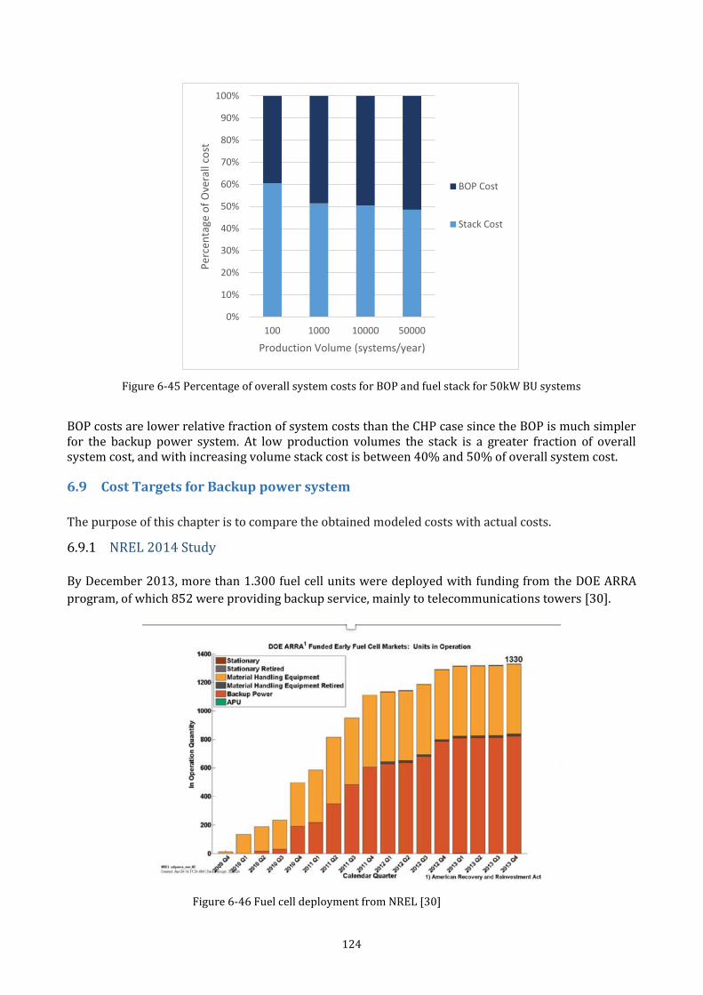
124
Figure 6-45 Percentage of overall system costs for BOP and fuel stack for 50kW BU systems
BOP costs are lower relative fraction of system costs than the CHP case since the BOP is much simpler for the backup power system. At low production volumes the stack is a greater fraction of overall system cost, and with increasing volume stack cost is between 40% and 50% of overall system cost.
6.9 Cost Targets for Backup power system
The purpose of this chapter is to compare the obtained modeled costs with actual costs.
6.9.1 NREL 2014 Study
By December 2013, more than 1.300 fuel cell units were deployed with funding from the DOE ARRA
program, of which 852 were providing backup service, mainly to telecommunications towers [30].
Figure 6-46 Fuel cell deployment from NREL [30]
0%
10%
20%
30%
40%
50%
60%
70%
80%
90%
100%
100 1000 10000 50000
Per
cen
tage
of
Ove
rall
cost
Production Volume (systems/year)
BOP Cost
Stack Cost
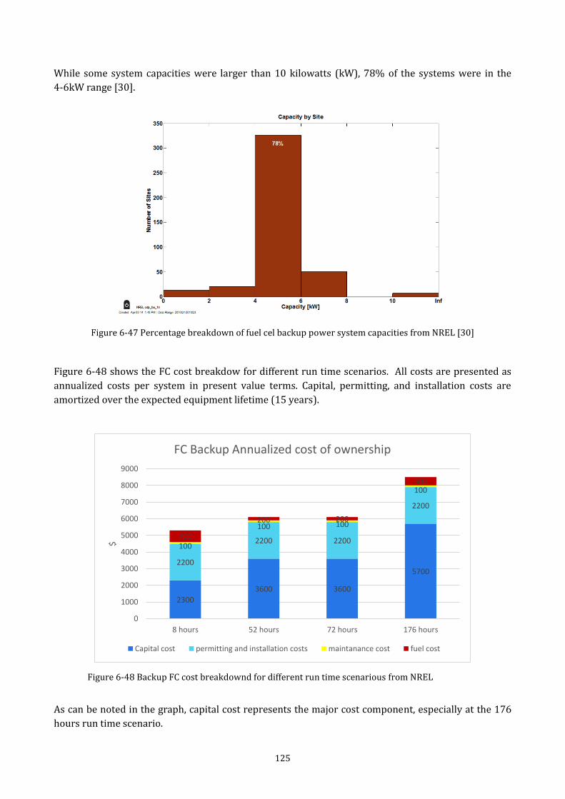
125
While some system capacities were larger than 10 kilowatts (kW), 78% of the systems were in the
4-6kW range [30].
Figure 6-47 Percentage breakdown of fuel cel backup power system capacities from NREL [30]
Figure 6-48 shows the FC cost breakdow for different run time scenarios. All costs are presented as
annualized costs per system in present value terms. Capital, permitting, and installation costs are
amortized over the expected equipment lifetime (15 years).
Figure 6-48 Backup FC cost breakdownd for different run time scenarious from NREL
As can be noted in the graph, capital cost represents the major cost component, especially at the 176
hours run time scenario.
2300
3600 3600
5700 2200
2200 2200
2200
100
100 100
100
700
200 200
500
0
1000
2000
3000
4000
5000
6000
7000
8000
9000
8 hours 52 hours 72 hours 176 hours
$
FC Backup Annualized cost of ownership
Capital cost permitting and installation costs maintanance cost fuel cost
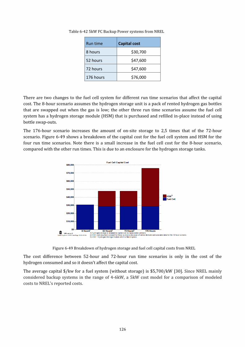
126
Table 6-42 5kW FC Backup Power systems from NREL
Run time Capital cost
8 hours $30,700
52 hours $47,600
72 hours $47,600
176 hours $76,000
There are two changes to the fuel cell system for different run time scenarios that affect the capital
cost. The 8-hour scenario assumes the hydrogen storage unit is a pack of rented hydrogen gas bottles
that are swapped out when the gas is low; the other three run time scenarios assume the fuel cell
system has a hydrogen storage module (HSM) that is purchased and refilled in-place instead of using
bottle swap-outs.
The 176-hour scenario increases the amount of on-site storage to 2,5 times that of the 72-hour
scenario. Figure 6-49 shows a breakdown of the capital cost for the fuel cell system and HSM for the
four run time scenarios. Note there is a small increase in the fuel cell cost for the 8-hour scenario,
compared with the other run times. This is due to an enclosure for the hydrogen storage tanks.
Figure 6-49 Breakdown of hydrogen storage and fuel cell capital costs from NREL
The cost difference between 52-hour and 72-hour run time scenarios is only in the cost of the
hydrogen consumed and so it doesn’t affect the capital cost.
The average capital $/kw for a fuel system (without storage) is $5,700/kW [30]. Since NREL mainly
considered backup systems in the range of 4-6kW, a 5kW cost model for a comparison of modeled
costs to NREL’s reported costs.
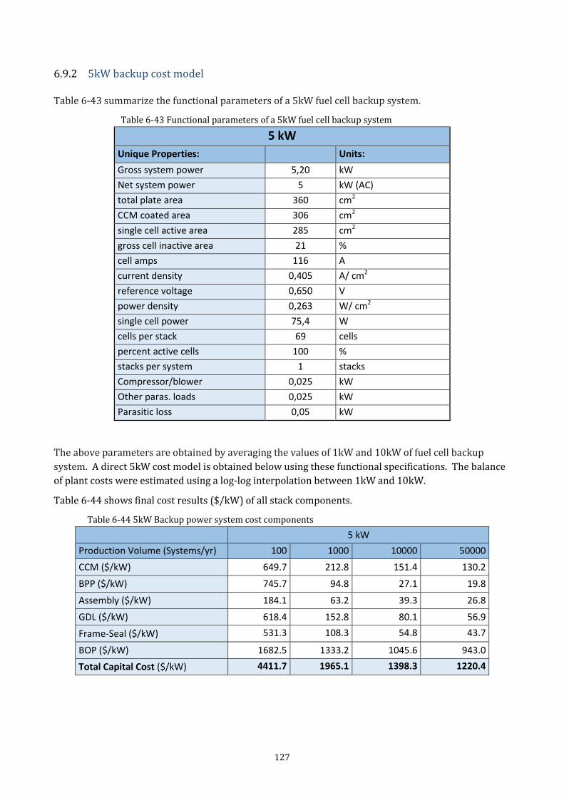
127
6.9.2 5kW backup cost model Table 6-43 summarize the functional parameters of a 5kW fuel cell backup system.
Table 6-43 Functional parameters of a 5kW fuel cell backup system
5 kW
Unique Properties: Units:
Gross system power 5,20 kW
Net system power 5 kW (AC)
total plate area 360 cm2
CCM coated area 306 cm2
single cell active area 285 cm2
gross cell inactive area 21 %
cell amps 116 A
current density 0,405 A/ cm2
reference voltage 0,650 V
power density 0,263 W/ cm2
single cell power 75,4 W
cells per stack 69 cells
percent active cells 100 %
stacks per system 1 stacks
Compressor/blower 0,025 kW
Other paras. loads 0,025 kW
Parasitic loss 0,05 kW
The above parameters are obtained by averaging the values of 1kW and 10kW of fuel cell backup
system. A direct 5kW cost model is obtained below using these functional specifications. The balance
of plant costs were estimated using a log-log interpolation between 1kW and 10kW.
Table 6-44 shows final cost results ($/kW) of all stack components.
Table 6-44 5kW Backup power system cost components
5 kW
Production Volume (Systems/yr) 100 1000 10000 50000
CCM ($/kW) 649.7 212.8 151.4 130.2
BPP ($/kW) 745.7 94.8 27.1 19.8
Assembly ($/kW) 184.1 63.2 39.3 26.8
GDL ($/kW) 618.4 152.8 80.1 56.9
Frame-Seal ($/kW) 531.3 108.3 54.8 43.7
BOP ($/kW) 1682.5 1333.2 1045.6 943.0
Total Capital Cost ($/kW) 4411.7 1965.1 1398.3 1220.4
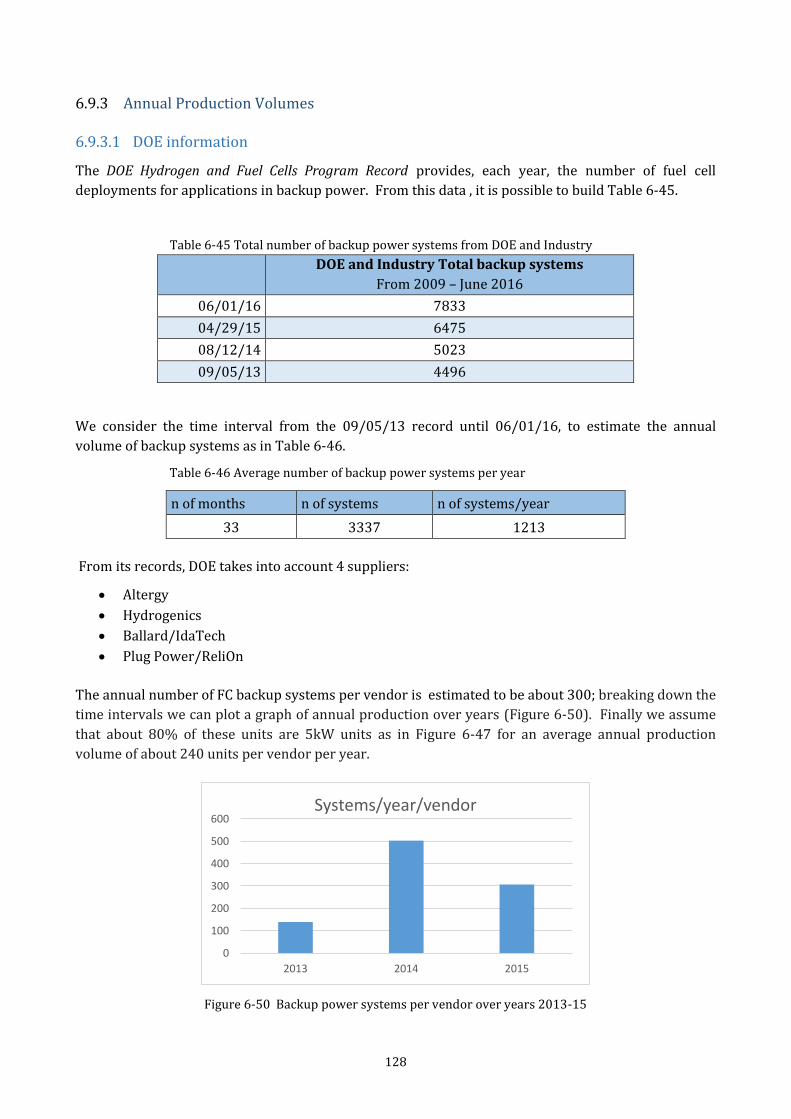
128
6.9.3 Annual Production Volumes
6.9.3.1 DOE information
The DOE Hydrogen and Fuel Cells Program Record provides, each year, the number of fuel cell
deployments for applications in backup power. From this data , it is possible to build Table 6-45.
Table 6-45 Total number of backup power systems from DOE and Industry
DOE and Industry Total backup systems
From 2009 – June 2016
06/01/16 7833
04/29/15 6475
08/12/14 5023
09/05/13 4496
We consider the time interval from the 09/05/13 record until 06/01/16, to estimate the annual
volume of backup systems as in Table 6-46.
Table 6-46 Average number of backup power systems per year
n of months n of systems n of systems/year
33 3337 1213
From its records, DOE takes into account 4 suppliers:
Altergy
Hydrogenics
Ballard/IdaTech
Plug Power/ReliOn
The annual number of FC backup systems per vendor is estimated to be about 300; breaking down the
time intervals we can plot a graph of annual production over years (Figure 6-50). Finally we assume
that about 80% of these units are 5kW units as in Figure 6-47 for an average annual production
volume of about 240 units per vendor per year.
Figure 6-50 Backup power systems per vendor over years 2013-15
0
100
200
300
400
500
600
2013 2014 2015
Systems/year/vendor
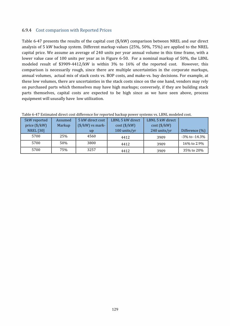
129
6.9.4 Cost comparison with Reported Prices Table 6-47 presents the results of the capital cost ($/kW) comparison between NREL and our direct
analysis of 5 kW backup system. Different markup values (25%, 50%, 75%) are applied to the NREL
capital price. We assume an average of 240 units per year annual volume in this time frame, with a
lower value case of 100 units per year as in Figure 6-50. For a nominal markup of 50%, the LBNL
modeled result of $3909-4412/kW is within 3% to 16% of the reported cost. However, this
comparison is necessarily rough, since there are multiple uncertainties in the corporate markups,
annual volumes, actual mix of stack costs vs. BOP costs, and make-vs. buy decisions. For example, at
these low volumes, there are uncertainties in the stack costs since on the one hand, vendors may rely
on purchased parts which themselves may have high markups; conversely, if they are building stack
parts themselves, capital costs are expected to be high since as we have seen above, process
equipment will ususally have low utilization.
Table 6-47 Estimated direct cost difference for reported backup power systems vs. LBNL modeled cost.
5kW reported
price ($/kW)
NREL [30]
Assumed
Markup
5 kW direct cost
($/kW) vs mark-
up
LBNL 5 kW direct
cost ($/kW)
100 units/yr
LBNL 5 kW direct
cost ($/kW)
240 units/yr Difference (%)
5700 25% 4560 4412 3909 -3% to -14.3%
5700 50% 3800 4412 3909 16% to 2.9%
5700 75% 3257 4412 3909 35% to 20%
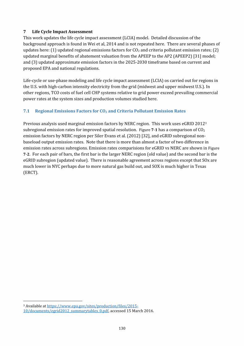
130
7 Life Cycle Impact Assessment
This work updates the life cycle impact assessment (LCIA) model. Detailed discussion of the
background approach is found in Wei et al, 2014 and is not repeated here. There are several phases of
updates here: (1) updated regional emissions factors for CO2 and criteria pollutant emission rates; (2)
updated marginal benefits of abatement valuation from the APEEP to the AP2 (APEEP2) [31] model;
and (3) updated approximate emission factors in the 2025-2030 timeframe based on current and
proposed EPA and national regulations.
Life-cycle or use-phase modeling and life cycle impact assessment (LCIA) os carried out for regions in
the U.S. with high-carbon intensity electricity from the grid (midwest and upper midwest U.S.). In
other regions, TCO costs of fuel cell CHP systems relative to grid power exceed prevailing commercial
power rates at the system sizes and production volumes studied here.
7.1 Regional Emissions Factors for CO2 and Criteria Pollutant Emission Rates
Previous analysis used marginal emission factors by NERC region. This work uses eGRID 20123
subregional emission rates for improved spatial resolution. Figure 7-1 has a comparison of CO2
emission factors by NERC region per Siler Evans et al. (2012) [32], and eGRID subregional non-
baseload output emission rates. Note that there is more than almost a factor of two difference in
emission rates across subregions. Emission rates comparisions for eGRID vs NERC are shown in Figure
7-2. For each pair of bars, the first bar is the larger NERC region (old value) and the second bar is the
eGRID subregion (updated value). There is reasonable agreement across regions except that SOx are
much lower in NYC perhaps due to more natural gas build out, and SOX is much higher in Texas
(ERCT).
3 Available at https://www.epa.gov/sites/production/files/2015-10/documents/egrid2012_summarytables_0.pdf, accessed 15 March 2016.
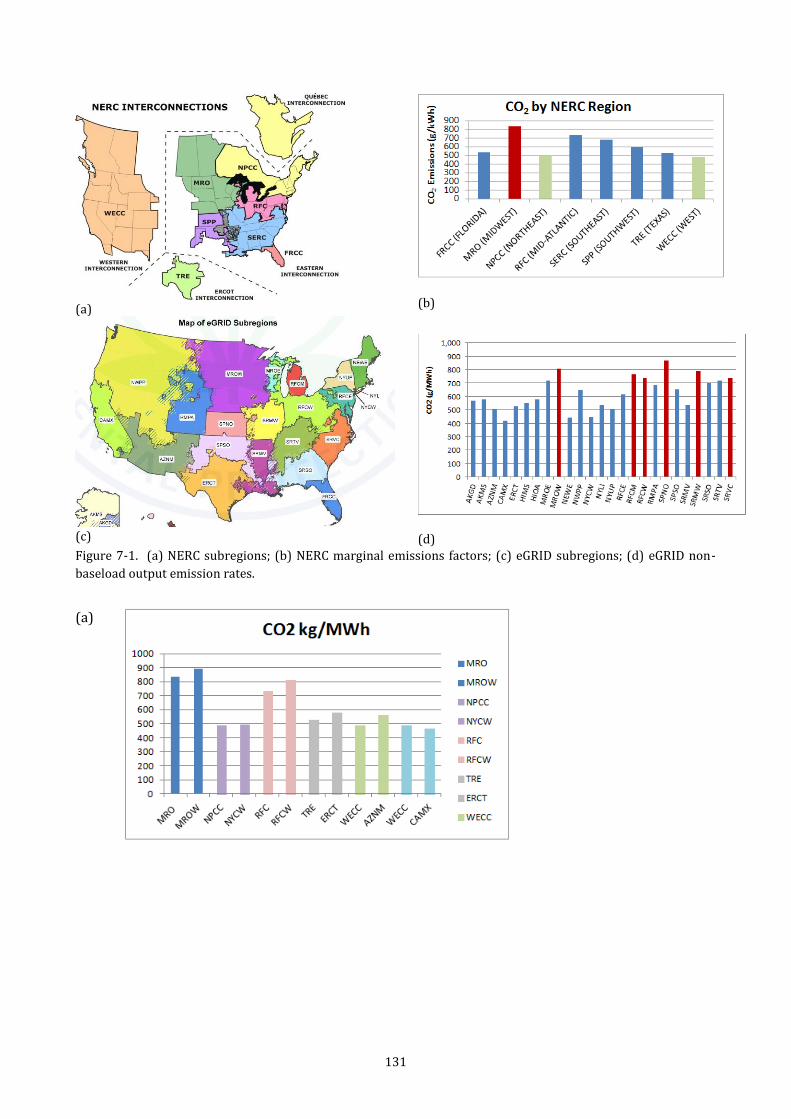
131
(a)
(b)
(c)
(d)
Figure 7-1. (a) NERC subregions; (b) NERC marginal emissions factors; (c) eGRID subregions; (d) eGRID non-
baseload output emission rates.
(a)
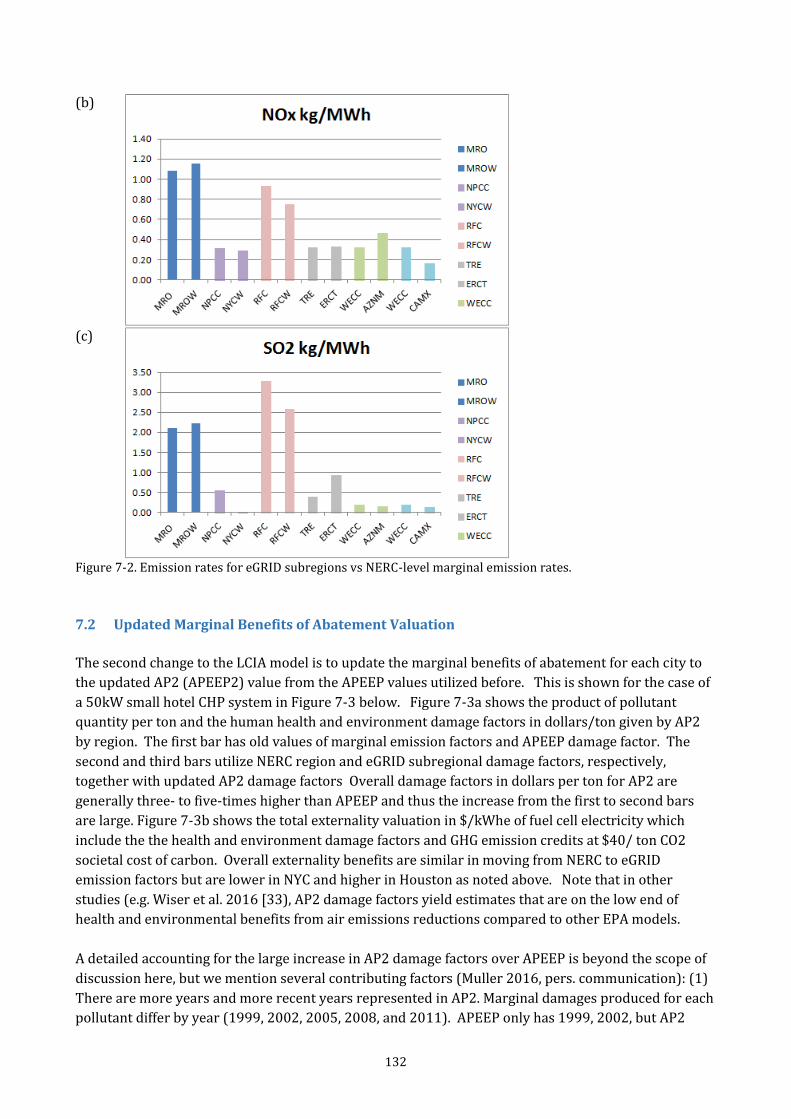
132
(b)
(c)
Figure 7-2. Emission rates for eGRID subregions vs NERC-level marginal emission rates.
7.2 Updated Marginal Benefits of Abatement Valuation
The second change to the LCIA model is to update the marginal benefits of abatement for each city to
the updated AP2 (APEEP2) value from the APEEP values utilized before. This is shown for the case of
a 50kW small hotel CHP system in Figure 7-3 below. Figure 7-3a shows the product of pollutant
quantity per ton and the human health and environment damage factors in dollars/ton given by AP2
by region. The first bar has old values of marginal emission factors and APEEP damage factor. The
second and third bars utilize NERC region and eGRID subregional damage factors, respectively,
together with updated AP2 damage factors Overall damage factors in dollars per ton for AP2 are
generally three- to five-times higher than APEEP and thus the increase from the first to second bars
are large. Figure 7-3b shows the total externality valuation in $/kWhe of fuel cell electricity which
include the the health and environment damage factors and GHG emission credits at $40/ ton CO2
societal cost of carbon. Overall externality benefits are similar in moving from NERC to eGRID
emission factors but are lower in NYC and higher in Houston as noted above. Note that in other
studies (e.g. Wiser et al. 2016 [33), AP2 damage factors yield estimates that are on the low end of
health and environmental benefits from air emissions reductions compared to other EPA models.
A detailed accounting for the large increase in AP2 damage factors over APEEP is beyond the scope of
discussion here, but we mention several contributing factors (Muller 2016, pers. communication): (1)
There are more years and more recent years represented in AP2. Marginal damages produced for each
pollutant differ by year (1999, 2002, 2005, 2008, and 2011). APEEP only has 1999, 2002, but AP2
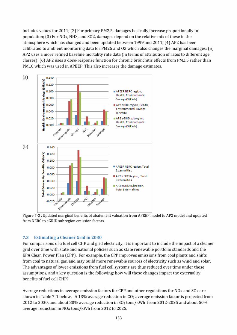
133
includes values for 2011; (2) For primary PM2.5, damages basically increase proportionally to
population; (3) For NOx, NH3, and SO2, damages depend on the relative mix of these in the
atmosphere which has changed and been updated between 1999 and 2011; (4) AP2 has been
calibrated to ambient monitoring data for PM25 and O3 which also changes the marginal damages; (5)
AP2 uses a more refined baseline mortality rate data (in terms of attribution of rates to different age
classes); (6) AP2 uses a dose-response function for chronic bronchitis effects from PM2.5 rather than
PM10 which was used in APEEP. This also increases the damage estimates.
(a)
(b)
Figure 7-3 . Updated marginal benefits of abatement valuation from APEEP model to AP2 model and updated
from NERC to eGRID subregion emission factors
7.3 Estimating a Cleaner Grid in 2030
For comparisons of a fuel cell CHP and grid electricity, it is important to include the impact of a cleaner
grid over time with state and national policies such as state renewable portfolio standards and the
EPA Clean Power Plan (CPP). For example, the CPP improves emissions from coal plants and shifts
from coal to natural gas, and may build more renewable sources of electricity such as wind and solar.
The advantages of lower emissions from fuel cell systems are thus reduced over time under these
assumptions, and a key question is the following: how will these changes impact the externality
benefits of fuel cell CHP?
Average reductions in average emission factors for CPP and other regulations for NOx and SOx are
shown in Table 7-1 below. A 13% average reduction in CO2 average emission factor is projected from
2012 to 2030, and about 80% average reduction in SO2 tons/kWh from 2012-2025 and about 50%
average reduction in NOx tons/kWh from 2012 to 2025.
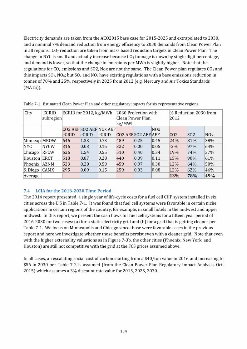
134
Electricity demands are taken from the AEO2015 base case for 2015-2025 and extrapolated to 2030,
and a nominal 7% demand reduction from energy efficiency to 2030 demands from Clean Power Plan
in all regions. CO2 reduction are taken from mass based reduction targets in Clean Power Plan. The
change in NYC is small and actually increase because CO2 tonnage is down by single digit percentage,
and demand is lower, so that the change in emissions per MWh is slightly higher. Note that the
regulations for CO2 emissions and SO2, Nox are not the same. The Clean Power plan regulates CO2 and
this impacts SO2, NOX; but SO2 and NOx have existing regulations with a base emissions reduction in
tonnes of 70% and 25%, respectively in 2025 from 2012 (e.g. Mercury and Air Toxics Standards
(MATS)).
Table 7-1. Estimated Clean Power Plan and other regulatory impacts for six representative regions
City EGRID subregion
EGRID for 2012, kg/MWh 2030 Projection with Clean Power Plan, kg/MWh
% Reduction 2030 from 2012
CO2 AEF eGRID
SO2 AEF eGRID
NOx AEF eGRID CO2 AEF SO2 AEF
NOx AEF CO2 SO2 NOx
Minneap. MROW 646 1.33 0.73 489 0.25 0.45 24% 81% 38%
NYC NYCW 316 0.03 0.15 322 0.00 0.05 -2% 97% 64%
Chicago RFCW 626 1.54 0.55 510 0.40 0.34 19% 74% 37%
Houston ERCT 518 0.87 0.28 440 0.09 0.11 15% 90% 61%
Phoenix AZNM 523 0.20 0.59 459 0.07 0.30 12% 64% 50%
S. Diego CAMX 295 0.09 0.15 259 0.03 0.08 12% 62% 46%
Average 13% 78% 49%
7.4 LCIA for the 2016-2030 Time Period
The 2014 report presented a single year of life-cycle costs for a fuel cell CHP system installed in six
cities across the U.S in Table 7-1. It was found that fuel cell systems were favorable in certain niche
applications in certain regions of the country, for example, in small hotels in the midwest and upper
midwest. In this report, we present the cash flows for fuel cell systems for a fifteen year period of
2016-2030 for two cases: (a) for a static electricity grid and (b) for a grid that is getting cleaner per
Table 7-1. We focus on Minneapolis and Chicago since those were favorable cases in the previous
report and here we investigate whether those benefits persist even with a cleaner grid. Note that even
with the higher externality valuations as in Figure 7-3b, the other cities (Phoenix, New York, and
Houston) are still not competitive with the grid at the FCS prices assumed above.
In all cases, an escalating social cost of carbon starting from a $40/ton value in 2016 and increasing to
$56 in 2030 per Table 7-2 is assumed (from the Clean Power Plan Regulatory Impact Analysis, Oct.
2015) which assumes a 3% discount rate value for 2015, 2025, 2030.
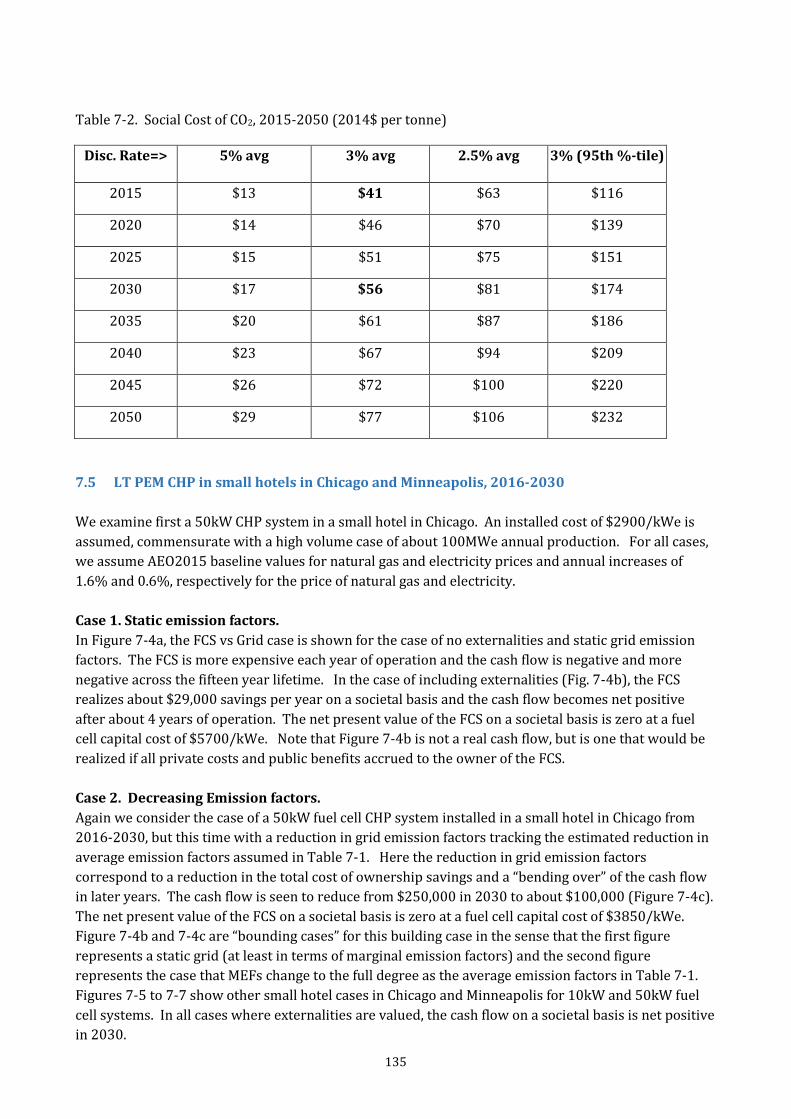
135
Table 7-2. Social Cost of CO2, 2015-2050 (2014$ per tonne)
Disc. Rate=> 5% avg 3% avg 2.5% avg 3% (95th %-tile)
2015 $13 $41 $63 $116
2020 $14 $46 $70 $139
2025 $15 $51 $75 $151
2030 $17 $56 $81 $174
2035 $20 $61 $87 $186
2040 $23 $67 $94 $209
2045 $26 $72 $100 $220
2050 $29 $77 $106 $232
7.5 LT PEM CHP in small hotels in Chicago and Minneapolis, 2016-2030
We examine first a 50kW CHP system in a small hotel in Chicago. An installed cost of $2900/kWe is
assumed, commensurate with a high volume case of about 100MWe annual production. For all cases,
we assume AEO2015 baseline values for natural gas and electricity prices and annual increases of
1.6% and 0.6%, respectively for the price of natural gas and electricity.
Case 1. Static emission factors.
In Figure 7-4a, the FCS vs Grid case is shown for the case of no externalities and static grid emission
factors. The FCS is more expensive each year of operation and the cash flow is negative and more
negative across the fifteen year lifetime. In the case of including externalities (Fig. 7-4b), the FCS
realizes about $29,000 savings per year on a societal basis and the cash flow becomes net positive
after about 4 years of operation. The net present value of the FCS on a societal basis is zero at a fuel
cell capital cost of $5700/kWe. Note that Figure 7-4b is not a real cash flow, but is one that would be
realized if all private costs and public benefits accrued to the owner of the FCS.
Case 2. Decreasing Emission factors.
Again we consider the case of a 50kW fuel cell CHP system installed in a small hotel in Chicago from
2016-2030, but this time with a reduction in grid emission factors tracking the estimated reduction in
average emission factors assumed in Table 7-1. Here the reduction in grid emission factors
correspond to a reduction in the total cost of ownership savings and a “bending over” of the cash flow
in later years. The cash flow is seen to reduce from $250,000 in 2030 to about $100,000 (Figure 7-4c).
The net present value of the FCS on a societal basis is zero at a fuel cell capital cost of $3850/kWe.
Figure 7-4b and 7-4c are “bounding cases” for this building case in the sense that the first figure
represents a static grid (at least in terms of marginal emission factors) and the second figure
represents the case that MEFs change to the full degree as the average emission factors in Table 7-1.
Figures 7-5 to 7-7 show other small hotel cases in Chicago and Minneapolis for 10kW and 50kW fuel
cell systems. In all cases where externalities are valued, the cash flow on a societal basis is net positive
in 2030.
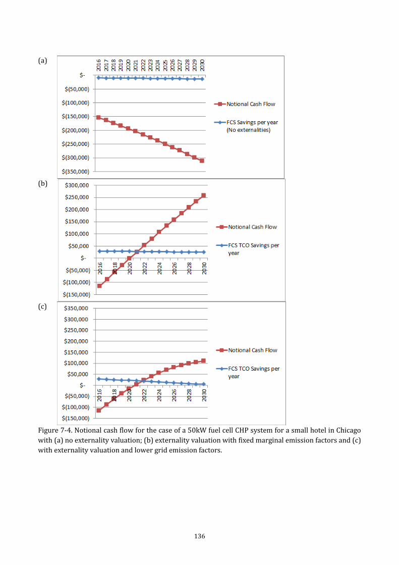
136
(a)
(b)
(c)
Figure 7-4. Notional cash flow for the case of a 50kW fuel cell CHP system for a small hotel in Chicago
with (a) no externality valuation; (b) externality valuation with fixed marginal emission factors and (c)
with externality valuation and lower grid emission factors.
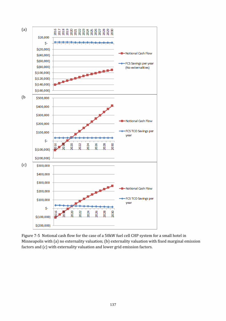
137
(a)
(b
(c)
Figure 7-5 Notional cash flow for the case of a 50kW fuel cell CHP system for a small hotel in
Minneapolis with (a) no externality valuation; (b) externality valuation with fixed marginal emission
factors and (c) with externality valuation and lower grid emission factors.
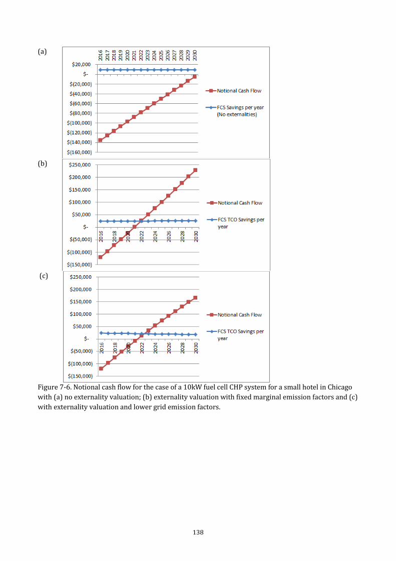
138
(a)
(b)
(c)
Figure 7-6. Notional cash flow for the case of a 10kW fuel cell CHP system for a small hotel in Chicago
with (a) no externality valuation; (b) externality valuation with fixed marginal emission factors and (c)
with externality valuation and lower grid emission factors.
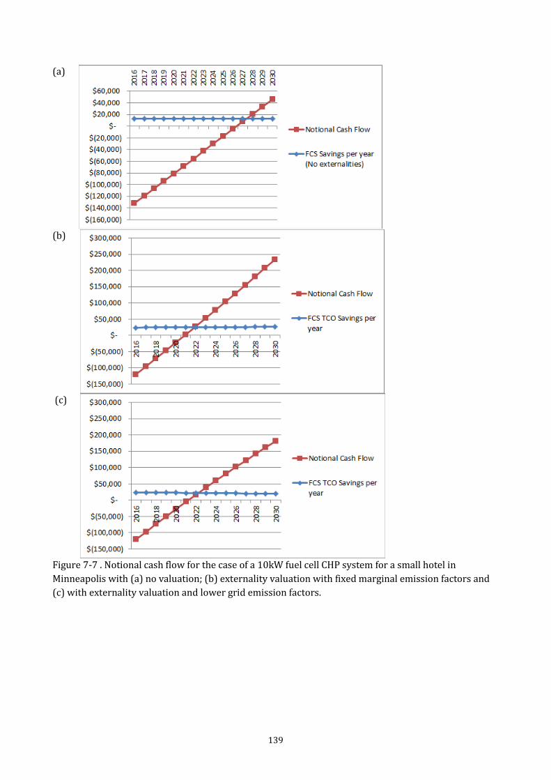
139
(a)
(b)
(c)
Figure 7-7 . Notional cash flow for the case of a 10kW fuel cell CHP system for a small hotel in
Minneapolis with (a) no valuation; (b) externality valuation with fixed marginal emission factors and
(c) with externality valuation and lower grid emission factors.
140
References
[1] M. Wei, T. Lipman, et al, “A Total Cost of Ownership Model for Low Temperature PEM Fuel Cells in Combined Heat and Power and Backup Power Applications,” Lawrence Berkeley National Laboratory Report LBNL- 6772E, October 2014.
[2] James, B., Spisak, A., Colella, W. Manufacturing Cost Analysis of Stationary Fuel Cell Systems, Strategic Analysis Inc. Arlington VA, September 2012.
[3] James, Brian, Kalinoski, J., and K. Baum. Mass-Production Cost Estimation for Automotive Fuel Cell Systems. 2010 Annual Merit Review Proceedings, Department of Energy, Hydrogen and Fuel Cells Program. Washington, D.C., June 2010.
[4] Sinha, Jayanti and Y. Yang. Direct Hydrogen PEMFC Manufacturing Cost Estimation for Automotive Applications. 2010 Annual Merit Review Proceedings, Department of Energy, Hydrogen and Fuel Cells Program. Washington, D.C., June 2010.
[5] Mahadevan, Kathya , V. Contini, M. Goshe, J. Price, F. Eubanks, and F. Griesemer. Economic Analysis of Stationary PEM Fuel Cell Systems. 2010 Annual Merit Review Proceedings, Department of Energy, Hydrogen and Fuel Cells Program. Washington, D.C., June 2010.
[6] D.L. Greene, K.G. Duleep, G. Upreti, Status and outlook for the U.S. non-automotive fuel cell industry: impacts of government policies and assessment of future opportunities, U.S. Department of Energy (2011); K. Mahadevan K. Judd H. Stone J. Zewatsky A. Thomas H. Mahy D. Paul, Identification and characterization of near-term direct hydrogen proton exchange membrane fuel cell markets, Apr. 2007.
[7] Stadler, Michael, Marnay, C., Gonçalo Cardoso, G. et al. The Carbon Dioxide Abatement Potential of California’s Mid-Sized Commercial Buildings. California Energy Commission, PIER Program. CEC‐500‐2010‐050 (2011).
[8] http://inhabitat.com/hyundai-hydrogen-powered-car-sets-new-eco-friendly-vehicle-record
[9] Nishizaki, K. and K. Hirai (2009), “Commercialization of residential PEM Fuel Cell CHP “ENE FARM,” White Paper by Tokyo Gas Co. and Osaka Gas Co.
[10] Haberl, J.S., (1994) “Economic Calculations for the ASHRAE Handbook,” Texas A&M University, College Station, Texas.
[11] J. Verrey, M.D. Wakeman, V. Michaud, J.-A.E. Månson, Manufacturing cost comparison of thermoplastic and thermoset RTM for an automotive floor pan, Composites Part A: Applied Science and Manufacturing, Volume 37, Issue 1, January 2006, Pages 9-22, ISSN 1359-835X, http://dx.doi.org/10.1016/j.compositesa.2005.05.048.
[12] ACI Technologies, Inc. “Manufacturing Fuel Cell Manhattan Project.” U.S. Government Contract No. N00014-08-D-0758, November 2011.
[13] Iannone R, Nenni ME (2013) Managing OEE to optimize factory performance. INTECH Open Access Publisher, Croatia
[14] R. Scataglini, A. Mayyas, M. Wei, S. H. Chan, T. Lipman, D. Gosselin, A. D’Alessio, H. Breunig, W. G. Colella, B. D. James, “A Total Cost of Ownership Model for Solid Oxide Fuel Cells in Combined Heat and Power and Power-Only Applications,” Lawrence Berkeley Laboratory Report LBNL-1005725. December 2015.
[15] R.A. Terpstra, P.P.A.C. Pex, A.H. de Vries, Ceramic Processing, Chapman and Hall, London, 1995
[16] A.J. Burggraaf, L. Cot, General overview, Trends and prospects, in: A.J. Burggraaf, L. Cot (Eds.), Fundamentals of Inorganic Membrane Science and Technology, Membrane Science and Technology Series, Vol. 4, 1996, pp. 1–19
[17] Wing, J. “Why fuel cells for telecom backup is a good call”, 2014,
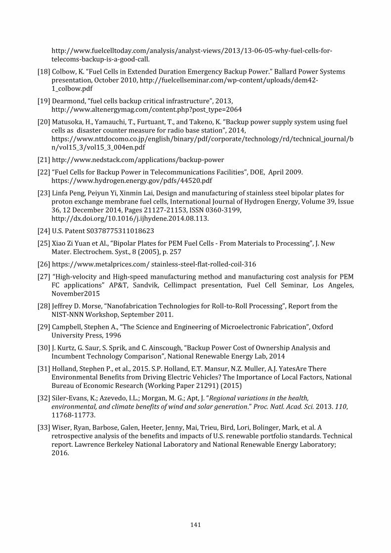
141
http://www.fuelcelltoday.com/analysis/analyst-views/2013/13-06-05-why-fuel-cells-for-telecoms-backup-is-a-good-call.
[18] Colbow, K. “Fuel Cells in Extended Duration Emergency Backup Power.” Ballard Power Systems presentation, October 2010, http://fuelcellseminar.com/wp-content/uploads/dem42-
1_colbow.pdf
[19] Dearmond, “fuel cells backup critical infrastructure”, 2013, http://www.altenergymag.com/content.php?post_type=2064
[20] Matusoka, H., Yamauchi, T., Furtuant, T., and Takeno, K. “Backup power supply system using fuel cells as disaster counter measure for radio base station”, 2014, https://www.nttdocomo.co.jp/english/binary/pdf/corporate/technology/rd/technical_journal/bn/vol15_3/vol15_3_004en.pdf
[21] http://www.nedstack.com/applications/backup-power
[22] “Fuel Cells for Backup Power in Telecommunications Facilities”, DOE, April 2009. https://www.hydrogen.energy.gov/pdfs/44520.pdf
[23] Linfa Peng, Peiyun Yi, Xinmin Lai, Design and manufacturing of stainless steel bipolar plates for proton exchange membrane fuel cells, International Journal of Hydrogen Energy, Volume 39, Issue 36, 12 December 2014, Pages 21127-21153, ISSN 0360-3199, http://dx.doi.org/10.1016/j.ijhydene.2014.08.113.
[24] U.S. Patent S0378775311018623
[25] Xiao Zi Yuan et Al., “Bipolar Plates for PEM Fuel Cells - From Materials to Processing”, J. New Mater. Electrochem. Syst., 8 (2005), p. 257
[26] https://www.metalprices.com/ stainless-steel-flat-rolled-coil-316
[27] “High-velocity and High-speed manufacturing method and manufacturing cost analysis for PEM FC applications” AP&T, Sandvik, Cellimpact presentation, Fuel Cell Seminar, Los Angeles, November2015
[28] Jeffrey D. Morse, “Nanofabrication Technologies for Roll-to-Roll Processing”, Report from the NIST-NNN Workshop, September 2011.
[29] Campbell, Stephen A., “The Science and Engineering of Microelectronic Fabrication”, Oxford University Press, 1996
[30] J. Kurtz, G. Saur, S. Sprik, and C. Ainscough, “Backup Power Cost of Ownership Analysis and Incumbent Technology Comparison”, National Renewable Energy Lab, 2014
[31] Holland, Stephen P., et al., 2015. S.P. Holland, E.T. Mansur, N.Z. Muller, A.J. YatesAre There Environmental Benefits from Driving Electric Vehicles? The Importance of Local Factors, National Bureau of Economic Research (Working Paper 21291) (2015)
[32] Siler-Evans, K.; Azevedo, I.L.; Morgan, M. G.; Apt, J. “Regional variations in the health, environmental, and climate benefits of wind and solar generation.” Proc. Natl. Acad. Sci. 2013. 110, 11768-11773.
[33] Wiser, Ryan, Barbose, Galen, Heeter, Jenny, Mai, Trieu, Bird, Lori, Bolinger, Mark, et al. A retrospective analysis of the benefits and impacts of U.S. renewable portfolio standards. Technical report. Lawrence Berkeley National Laboratory and National Renewable Energy Laboratory; 2016.
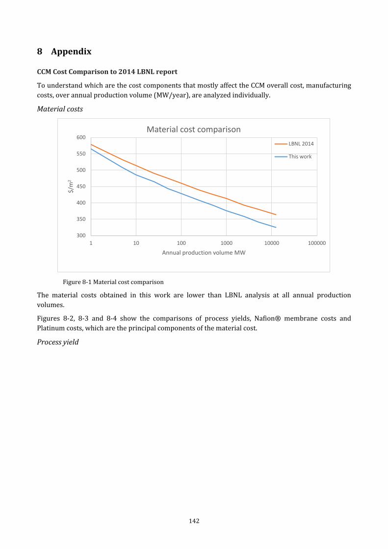
142
8 Appendix
CCM Cost Comparison to 2014 LBNL report
To understand which are the cost components that mostly affect the CCM overall cost, manufacturing
costs, over annual production volume (MW/year), are analyzed individually.
Material costs
Figure 8-1 Material cost comparison
The material costs obtained in this work are lower than LBNL analysis at all annual production
volumes.
Figures 8-2, 8-3 and 8-4 show the comparisons of process yields, Nafion® membrane costs and
Platinum costs, which are the principal components of the material cost.
Process yield
300
350
400
450
500
550
600
1 10 100 1000 10000 100000
$/m
2
Annual production volume MW
Material cost comparison
LBNL 2014
This work
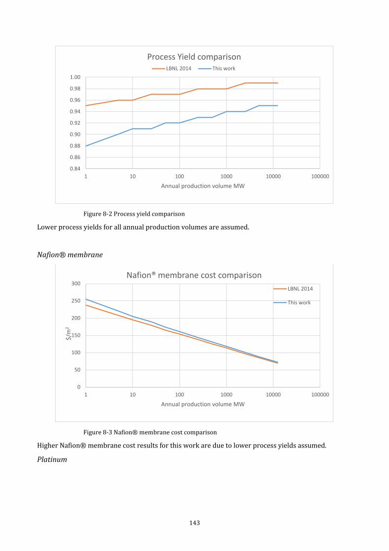
143
Figure 8-2 Process yield comparison
Lower process yields for all annual production volumes are assumed.
Nafion® membrane
Figure 8-3 Nafion® membrane cost comparison
Higher Nafion® membrane cost results for this work are due to lower process yields assumed.
Platinum
0.84
0.86
0.88
0.90
0.92
0.94
0.96
0.98
1.00
1 10 100 1000 10000 100000
Annual production volume MW
Process Yield comparison LBNL 2014 This work
0
50
100
150
200
250
300
1 10 100 1000 10000 100000
$/m
2
Annual production volume MW
Nafion® membrane cost comparison
LBNL 2014
This work
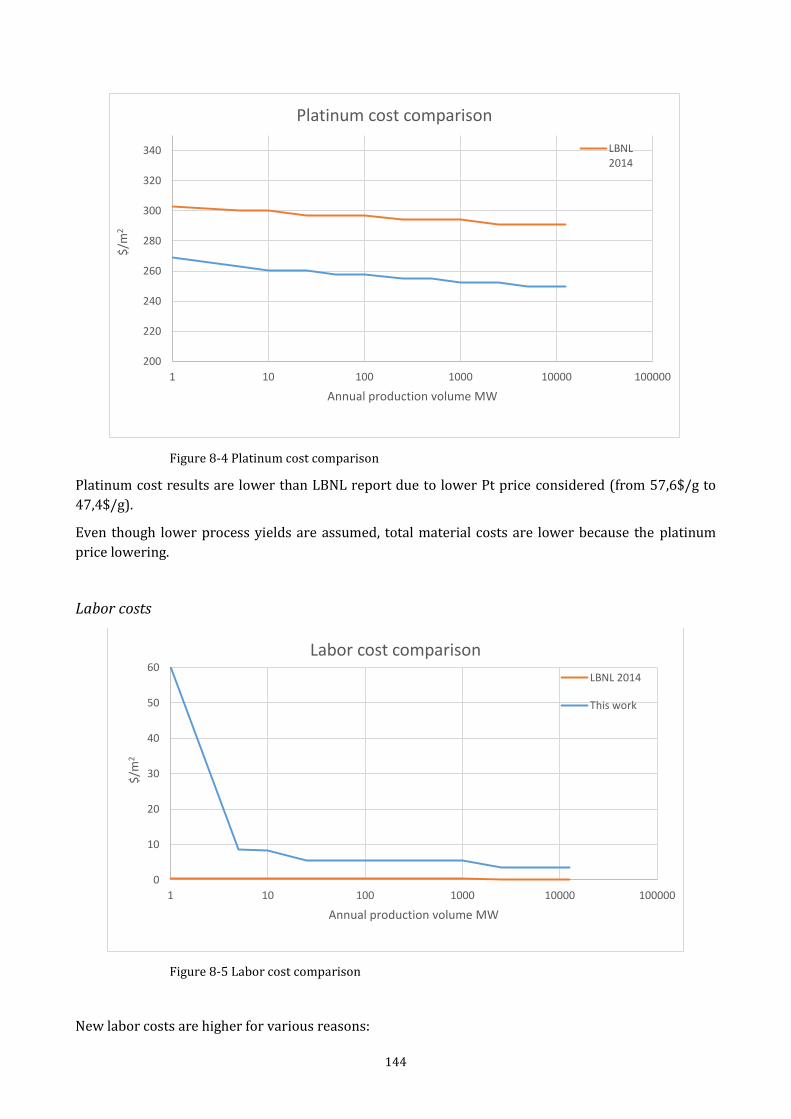
144
Figure 8-4 Platinum cost comparison
Platinum cost results are lower than LBNL report due to lower Pt price considered (from 57,6$/g to
47,4$/g).
Even though lower process yields are assumed, total material costs are lower because the platinum
price lowering.
Labor costs
Figure 8-5 Labor cost comparison
New labor costs are higher for various reasons:
200
220
240
260
280
300
320
340
1 10 100 1000 10000 100000
$/m
2
Annual production volume MW
Platinum cost comparison
LBNL2014
0
10
20
30
40
50
60
1 10 100 1000 10000 100000
$/m
2
Annual production volume MW
Labor cost comparison
LBNL 2014
This work
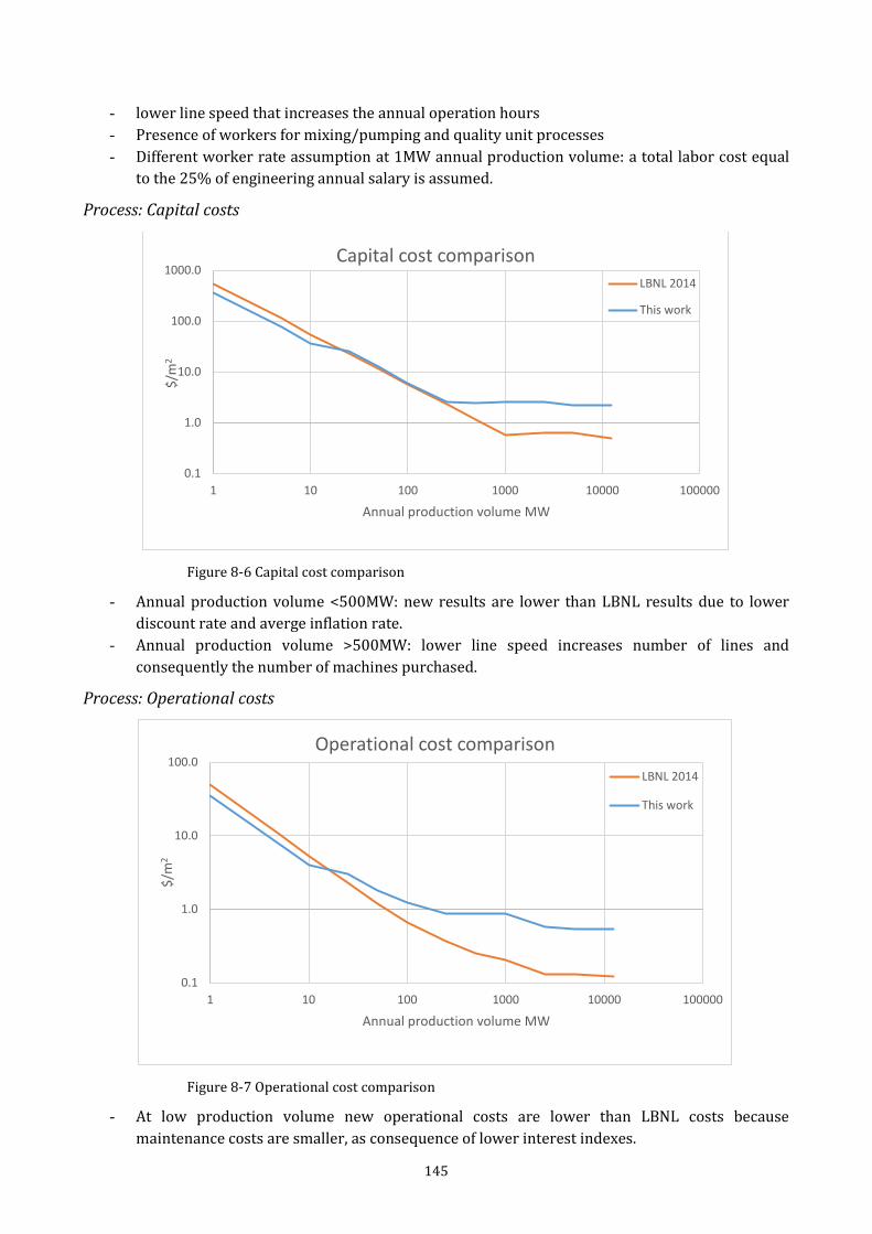
145
- lower line speed that increases the annual operation hours
- Presence of workers for mixing/pumping and quality unit processes
- Different worker rate assumption at 1MW annual production volume: a total labor cost equal
to the 25% of engineering annual salary is assumed.
Process: Capital costs
Figure 8-6 Capital cost comparison
- Annual production volume <500MW: new results are lower than LBNL results due to lower
discount rate and averge inflation rate.
- Annual production volume >500MW: lower line speed increases number of lines and
consequently the number of machines purchased.
Process: Operational costs
Figure 8-7 Operational cost comparison
- At low production volume new operational costs are lower than LBNL costs because
maintenance costs are smaller, as consequence of lower interest indexes.
0.1
1.0
10.0
100.0
1000.0
1 10 100 1000 10000 100000
$/m
2
Annual production volume MW
Capital cost comparison LBNL 2014
This work
0.1
1.0
10.0
100.0
1 10 100 1000 10000 100000
$/m
2
Annual production volume MW
Operational cost comparison
LBNL 2014
This work
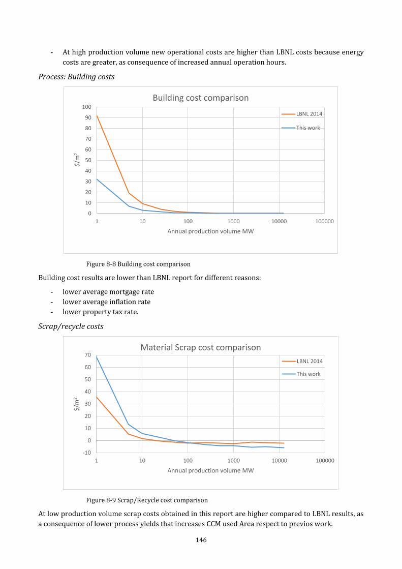
146
- At high production volume new operational costs are higher than LBNL costs because energy
costs are greater, as consequence of increased annual operation hours.
Process: Building costs
Figure 8-8 Building cost comparison
Building cost results are lower than LBNL report for different reasons:
- lower average mortgage rate
- lower average inflation rate
- lower property tax rate.
Scrap/recycle costs
Figure 8-9 Scrap/Recycle cost comparison
At low production volume scrap costs obtained in this report are higher compared to LBNL results, as
a consequence of lower process yields that increases CCM used Area respect to previos work.
0
10
20
30
40
50
60
70
80
90
100
1 10 100 1000 10000 100000
$/m
2
Annual production volume MW
Building cost comparison
LBNL 2014
This work
-10
0
10
20
30
40
50
60
70
1 10 100 1000 10000 100000
$/m
2
Annual production volume MW
Material Scrap cost comparison
LBNL 2014
This work
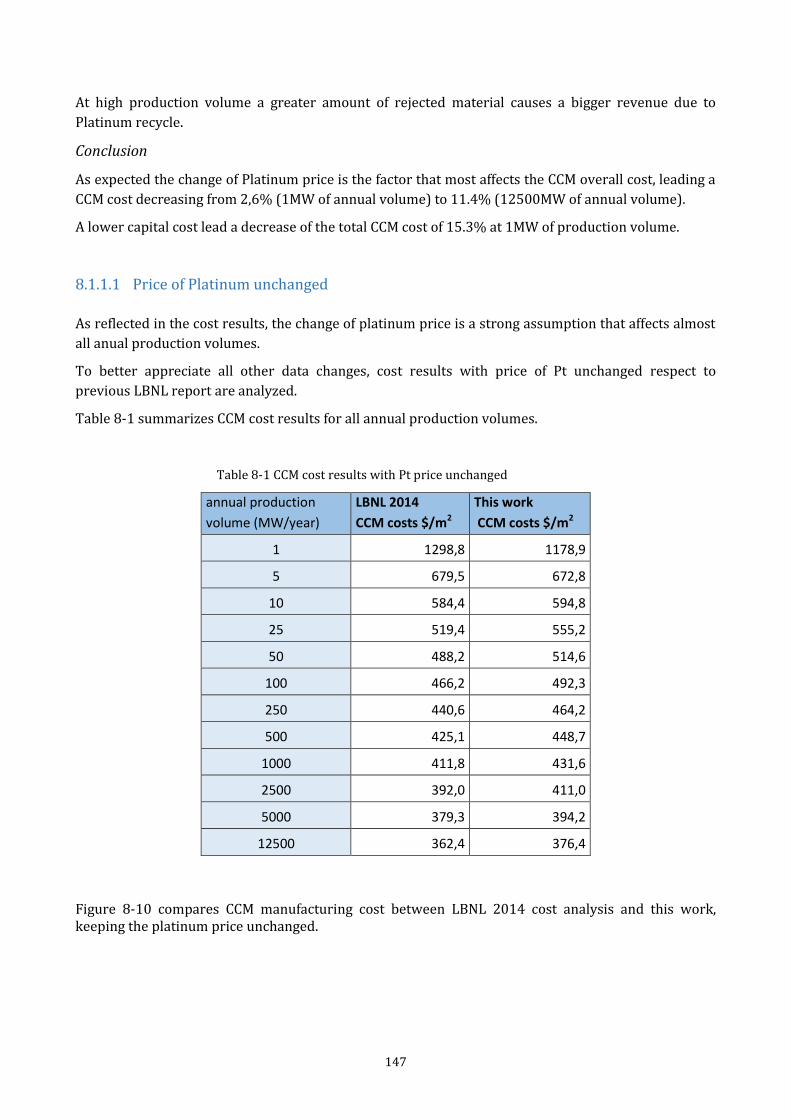
147
At high production volume a greater amount of rejected material causes a bigger revenue due to
Platinum recycle.
Conclusion
As expected the change of Platinum price is the factor that most affects the CCM overall cost, leading a
CCM cost decreasing from 2,6% (1MW of annual volume) to 11.4% (12500MW of annual volume).
A lower capital cost lead a decrease of the total CCM cost of 15.3% at 1MW of production volume.
8.1.1.1 Price of Platinum unchanged
As reflected in the cost results, the change of platinum price is a strong assumption that affects almost
all anual production volumes.
To better appreciate all other data changes, cost results with price of Pt unchanged respect to
previous LBNL report are analyzed.
Table 8-1 summarizes CCM cost results for all annual production volumes.
Table 8-1 CCM cost results with Pt price unchanged
annual production
volume (MW/year)
LBNL 2014
CCM costs $/m2
This work
CCM costs $/m2
1 1298,8 1178,9
5 679,5 672,8
10 584,4 594,8
25 519,4 555,2
50 488,2 514,6
100 466,2 492,3
250 440,6 464,2
500 425,1 448,7
1000 411,8 431,6
2500 392,0 411,0
5000 379,3 394,2
12500 362,4 376,4
Figure 8-10 compares CCM manufacturing cost between LBNL 2014 cost analysis and this work, keeping the platinum price unchanged.
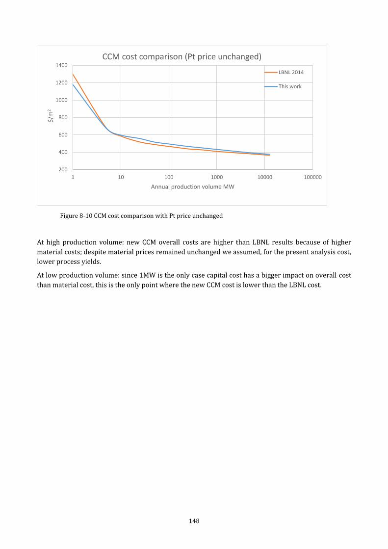
148
Figure 8-10 CCM cost comparison with Pt price unchanged
At high production volume: new CCM overall costs are higher than LBNL results because of higher
material costs; despite material prices remained unchanged we assumed, for the present analysis cost,
lower process yields.
At low production volume: since 1MW is the only case capital cost has a bigger impact on overall cost
than material cost, this is the only point where the new CCM cost is lower than the LBNL cost.
200
400
600
800
1000
1200
1400
1 10 100 1000 10000 100000
$/m
2
Annual production volume MW
CCM cost comparison (Pt price unchanged)
LBNL 2014
This work