Barcelona GSE Working Paper Series

Working Paper nº 606

A Tractable Consideration Set Structure for Network Revenue Management

Arne K. Strauss Kalyan Talluri

This version: October 2012 (February 2012)

A tractable consideration set structure for network revenue

management

Arne K. Strauss∗, Kalyan Talluri†

26 October 2012

Abstract

Models incorporating more realistic models of customer behavior, as customers choosing from an offer

set, have recently become popular in assortment optimization and revenue management. The dynamic

program for these models is intractable and approximated by a deterministic linear program called the

CDLP which has an exponential number of columns. When there are products that are being considered

for purchase by more than one customer segment, CDLP is difficult to solve since column generation

is known to be NP-hard. However, recent research indicates that a formulation based on segments with

cuts imposing consistency (SDCP+) is tractable and approximates the CDLP value very closely. In this

paper we investigate the structure of the consideration sets that make the two formulations exactly equal.

We show that if the segment consideration sets follow a tree structure, CDLP = SDCP+. We give a

counterexample to show that cycles can induce a gap between the CDLP and the SDCP+ relaxation.

We derive two classes of valid inequalities called flow and synchronization inequalities to further improve

(SDCP+), based on cycles in the consideration set structure. We give a numeric study showing the

performance of these cycle-based cuts.

Keywords: discrete-choice models, network revenue management, consideration sets

1 Introduction and literature review

Revenue management (RM) is the control of the sale of a limited quantity of a resource (hotel rooms for a

night, airline seats, advertising slots etc.) to a heterogenous population with different valuations for a unit

of the resource. The resource is perishable, and for simplicity’s sake, we assume that it perishes at a fixed

point of time in the future. Customers are independent of each other and arrive randomly during a sale

period, and demand one unit of resource each. Sale is online, and the firm has to decide which products at

∗Warwick Business School, University of Warwick, Coventry CV4 7AL, United Kingdom. email:arne.strauss@wbs.ac.uk†ICREA & Universitat Pompeu Fabra, Ramon Trias Fargas 25-27, 08005 Barcelona, Spain. email:kalyan.talluri@upf.edu

1

what price it should offer, the tradeoff being selling too much at too low a price early and running out of

capacity, or, losing too many price-sensitive customers and ending up with excess unsold inventory.

In industries such as hotels, airlines and media, the products consume bundles of different resources

(multi-night stays, multi-leg itineraries) and the decision on whether to offer a particular product at a certain

price depends on the expected future demand and current inventory levels for all the resources used by the

product, and hence indirectly, all the resources in the network. Network revenue management (network RM)

is control based on the demands for the entire network. Chapter 3 of Talluri and van Ryzin [16] contains all

the necessary background on network RM.

RM incorporating more realistic models of customer behavior, as customers choosing from an offer set,

have recently become popular (Talluri and van Ryzin [15], Gallego, Iyengar, Phillips, and Dubey [5], Liu and

van Ryzin [9], Kunnumkal and Topaloglu [8], Zhang and Adelman [18], Meissner and Strauss [10], Bodea,

Ferguson, and Garrow [2], Bront, Mendez-Dıaz, and Vulcano [3], Mendez-Dıaz, Bront, Vulcano, and Zabala

[12], Kunnumkal [7]).

Gallego et al. [5] and Liu and van Ryzin [9] propose a linear program called Choice Deterministic Linear

Program (CDLP ), while Talluri [17] developed a formulation called Segment-based Deterministic Concave

Program (SDCP ) that is weaker than the upper bound resulting from the CDLP but coincides for non-

overlapping segment consideration sets. Gallego, Ratcliff, and Shebalov [6] taking a similar approach, but

specialized to the multinomial logit (MNL) model of choice, propose a compact linear program called the Sales

Based Linear Program (SBLP ) that also coincides with CDLP for non-overlapping segment consideration

sets.

The size of the CDLP formulation grows exponentially in the number of products, and the solution

strategy is to use column generation; but finding an entering column is NP-hard even in restrictive cases

such as the MNL model of choice with just two segments and overlapping consideration sets (Bront et al.

[3], Rusmevichientong, Shmoys, and Topaloglu [13]).

SDCP is tractable when consideration sets are small, but its performance is poor when segment con-

sideration sets overlap (i.e., the bound is significantly looser than CDLP ). Meissner, Strauss, and Talluri

[11] extend the SDCP formulation, that we call SDCP+ here, to obtain progressively tighter relaxations

of CDLP for the case of overlapping consideration sets by adding product cuts that interpret the linear

programming decision variables as randomization rules. These constraints are easy to generate and work for

general discrete-choice models. Talluri [17] specializes the SBLP formulation of Gallego et al. [6] to obtain

a more compact formulation (that we call SBLP+) that is exponential only in the size of the intersections

of the consideration sets. In numerical testing SDCP+ and SBLP+ achieve the CDLP value in many

instances despite being an order of magnitude more compact.

This paper is an attempt to understand when the optimal value of the relatively compact SDCP+

relaxation (and SBLP+ for the MNL model) achieves the intractable CDLP formulation value. We show

that if the segment consideration sets follow a certain tree structure, the two problems are equivalent, and

give a counterexample to show that cycles can induce a gap between CDLP and the SDCP+ relaxation.

2

We then derive valid inequalities for the dynamic program based on cycles in the consideration set structure.

We give a numeric study showing the performance of these cycle-based cuts.

The remainder of the paper is organized as follows: In §2 we introduce the notation, the demand model

and the basic dynamic program. In §3 we state the two approximations of the dynamic program, namely

the CDLP and the SDCP+, followed by the main structural results that we prove in this paper. In §4 we

illustrate the approximations on a numerical example from the literature. In §5 we show two applications

from sports RM and buy-up modeling where the segment consideration set structure is a tree as in our

structural result. In §6 we describe two classes of cuts based on cycles in the consideration set graph, and

test their performance in §7. In §8 we summarize our conclusions.

2 Model and notation

A product is a specification of a price and a combination of resources to be consumed. For example, a

product could be an itinerary-fare class combination for an airline network, where the sale of a seat for an

itinerary consumes one seat each on a set of flight legs (the resources); likewise, in a hotel network a product

would be a multi-night stay for a particular room type at a certain price point. Time is discrete and assumed

to consist of T intervals, indexed by t. We assume that the booking horizon begins at time 0 and that all the

resources perish instantaneously at time T . We make the standard assumption that the time intervals are

fine enough so that the probability of more than one customer arriving in any single time period is negligible.

The underlying network has m resources (indexed by i) and n products (indexed by j), and we refer to

the set of all resources as I and the set of all products as J . A product j uses a subset of resources, and is

identified (possibly) with a set of sale restrictions or features and a revenue of rj . The resources used by j

are represented by aij = 1 if product j uses resource i, and aij = 0 otherwise, or alternately with the 0-1

incidence vector ~Aj of product j. Let A denote the resource-product incidence matrix; columns of A are

then ~Aj . We denote the vector of capacities at time t as ~ct, so the initial set of capacities at time 0 is ~c0.

The vector ~1 is a vector of all ones, and ~0 is a vector of all zeroes (dimension appropriate to the context).

We assume there are L := {1, . . . , L} customer segments, each with distinct purchase behavior. In each

period, there is a customer arrival with probability λ. A customer belongs to segment l with probability

pl. We denote λl = plλ and assume∑

l∈L pl = 1, so λ =∑

l∈L λl. We are assuming time-homogenous

arrivals (homogenous in rates and segment mix), but the model and all solution methods in this paper

can be transparently extended to the case when rates and mix change by period. Each segment l has a

consideration set Cl ⊆ J of products that it considers for purchase (see [14] for a survey on consideration set

literature). We assume this consideration set is known to the firm (by a previous process of estimation and

analysis), and the consideration sets for different segments can overlap.

In each period the firm offers a subset S of its products for sale, called the offer set. Given an offer set S,

an arriving customer purchases a product j in the set S or decides not to purchase. The no-purchase option

is indexed by 0 and is always present for the customer.

3

A segment-l customer is indifferent to a product outside his consideration set; i.e., his choice probabilities

are not affected by the availability of products j ∈ J \Cl. A segment-l customer purchases j ∈ S with given

probability P lj (S). This is a set-function defined on all subsets of J . For the moment we assume these set

functions are given by an oracle; it could conceivably be given by a simple formula as in the MNL model.

Whenever we specify probabilities for a segment l for a given offer set S, we just write it with respect to

Sl|S := Cl ∩ S (note that P lj (S) = P l

j(Sl|S)). We define the vector ~P l(S) = [P l1(Sl|S), . . . , P l

n(Sl|S)] (recall

the no-purchase option is indexed by 0, so it is not included in this vector).

Given a customer arrival, and an offer set S, the firm sells j ∈ S with probability Pj(S) =∑

l∈L plPlj(Sl|S)

and makes no sale with probability P0(S) = 1−∑

j∈S Pj(S). We define the vector ~P (S) = [P1(S), . . . , Pn(S)].

Notice that ~P (S) =∑

l∈L pl ~Pl(S). We define the vectors ~Ql(S) = A~P l(S) and ~Q(S) = A~P (S). The revenue

functions can be written as Rl(S) =∑

j∈SlrjP

lj (Sl|S) and R(S) =

∑

j∈S rjPj(S).

Let Vt(~ct) denote the maximum expected revenue that can be earned over the remaining time horizon

[t, T ], given remaining capacity ~ct in period t. Then Vt(~ct) must satisfy the Bellman equation

Vt(~ct) = maxS⊆J(~ct)

∑

j∈S

λPj(S)(

rj + Vt+1(~ct − ~Aj))

+(

λP0(S) + 1− λ)

Vt+1(~ct)

, ∀ t, ∀~ct, (1)

with the boundary condition VT (~cT ) = 0 for all ~cT . The set J(~ct) contains all products that can be feasibly

offered given remaining available capacity: J(~ct) := {j ∈ J | ~Aj ≤ ~ct}. Let V DP := V0(~c0) denote the optimal

value of this dynamic program from 0 to T , for the given initial capacity vector ~c0.

In our notation and demand model we broadly follow Bront et al. [3] and Liu and van Ryzin [9].

3 Approximations

We give the two formulations that we consider in this paper. Both can be seen as relaxations of (1).

4

3.1 Choice Deterministic Linear Program (CDLP )

The choice-based deterministic linear program (CDLP ) defined in Gallego et al. [5] and Liu and van Ryzin

[9] is as follows:

max∑

S⊆J

λR(S)wS (2)

s.t.∑

S⊆J

λwS~Q(S) ≤ ~c0

(CDLP )∑

S⊆J

wS = T

0 ≤ wS , ∀S ⊆ J.

The formulation has 2n variables wS that can be interpreted as the fraction of time set S is offered (including

w{∅}). Liu and van Ryzin [9] show that the optimal objective value is an upper bound on V DP . They also

show that the problem can be solved efficiently by column-generation for the MNL model and non-overlapping

segments. Bront et al. [3] and Rusmevichientong et al. [13] investigate this further and show that column

generation is NP-hard whenever the consideration sets for the segments overlap, even for the MNL choice

model.

3.2 Enhanced Segment-Based Deterministic Concave Program (SDCP+)

Talluri [17] proposed an upper bound on CDLP called the segment-based deterministic concave program

(SDCP ) that coincides with the CDLP when the segments do not overlap. The SDCP corresponds to the

formulation (SDCP+) given below without the equations (3). In applications, the segments’ consideration

sets can overlap in a variety of ways, and the choice probabilities depend on the offer set, and need not

follow any structure. Meissner et al. [11] develop a set of valid inequalities for SDCP called product cuts as

defined in (3) that tighten SDCP , and we call the combined formulation (SDCP+):

5

max

L∑

l=1

∑

Sl⊆Cl

λlRl(Sl)w

lSl

s.t.

(SDCP+)

L∑

l=1

~yl ≤ ~c0

∑

Sl⊆Cl

λl~Ql(Sl)w

lSl

≤ ~yl, ∀ l ∈ L

∑

Sl⊆Cl

wlSl

= T, ∀ l ∈ L

~yl ≤ λlT~1, ∀ l ∈ L∑

{Sl⊆Cl|Sl⊇Slm}

wlSl

−∑

{Sm⊆Cm|Sm⊇Slm}

wmSm

= 0,

∀Slm ⊆ Cl ∩ Cm, ∀ {l,m} ⊂ L : Cl ∩ Cm 6= ∅ (3)

wlSl

≥ 0, ∀Sl ⊆ Cl, ∀ l ∈ L,

~yl ≥ ~0, ∀ l ∈ L.

The product cuts are valid in the sense that adding them to (SDCP ) still results in an upper bound

on the stochastic dynamic program (1). The number of these cuts depends on the size of the overlap of

consideration sets, and can be enumerated when overlaps are small. Even otherwise, one can add the cuts

selectively, say restricting to the case where |Slm| is 2 or 3. The number of variables depends on the size of

the consideration sets themselves, and can likewise be enumerated if consideration sets are small.

We state the following proposition whose proof is trivial:

Proposition 1. If two segments have identical consideration sets, we can merge the two segments into one,

changing Rl(Sl) and Ql(Sl) as the expected revenue and resource consumption for the two segments combined,

without altering the solution of (SDCP+).

Therefore, whenever two segments have identical consideration sets, we merge them and consider a merged

segment.

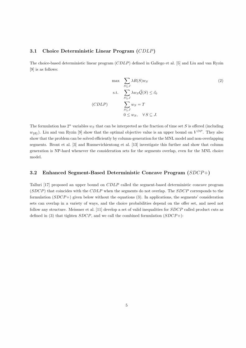
3.3 Example showing gap between CDLP and SDCP+

Figure 1 shows an example with five products and three segments and their respective consideration sets.

For this example we show that there is a gap between the optimal objective values of SDCP+ and CDLP .

Assume T = 1, capacity c = 1, revenue rj = 1 for all products j ∈ J = {1, 2, 3, 4, 5}, λl = 1/3 for all

segments l ∈ {A,B,C}, and the purchase probabilities defined as follows: PAj ({1, 2}) := 0.5 for j = 1, 2,

PAj ({2, 5}) := 0.5 for j = 2, 5, PB

2 ({2}) := 1, PBj ({1, 2, 3}) := 1/3 for j = 1, 2, 3, PC

4 ({4}) := 1 and

6

A

B

C

1

2

34

5

Figure 1: Consideration sets for 3 segments, 5 products

PCj ({3, 5}) := 0.5 for j = 3, 5, and 0 for all other sets.

Claim: There is a feasible solution to SDCP+ for this network with objective value 1.

Proof

For this data, an optimal solution to SDCP+ is given by yl = 1/3 for all segments l, and wA{1,2} = wA

{2,5} =

0.5, wB{2} = wB

{1,2,3} = 0.5, wC{4} = wC

{3,5} = 0.5, and wlSl

= 0 otherwise for all l ∈ {A,B,C}, Sl ⊂ Cl. This

solution is feasible to (SDCP+) since λl

∑

Sl⊆ClQl(Sl)w

lSl

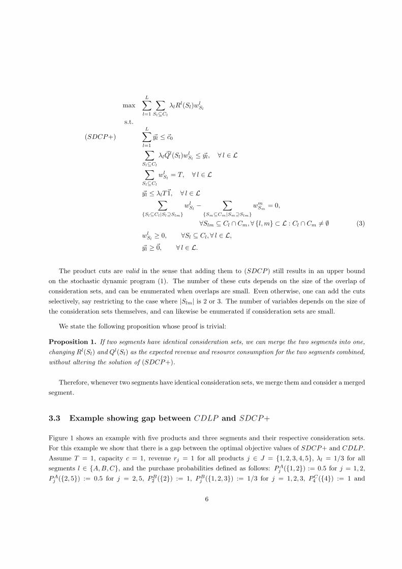
= 1/3 = yl for all segments l, the product cuts

(3) for all pairs of segments {l,m} and sets Slm ⊂ Cl∩Cm, Slm 6= ∅, are satisfied as reported in Table 1, and

they also hold for Slm = ∅ since the solution satisfies∑

Sl⊆Clwl

Sl= 1 for all segments l. The other constraints

are likewise satisfied as can easily be checked. The objective value is 1 since λl

∑

Sl⊆ClRl(Sl)w

lSl

= 1/3 for

each l ∈ {A,B,C}.

✷

{l,m} Slm Sl ⊇ Slm

∑

Sl⊇Slmwl

SlSm ⊇ Slm

∑

Sm⊇Slmwm

Sm

{A,B} {1} {1},{1,2},{1,5},{1,2,5} 0.5 {1},{1,2},{1,3},{1,2,3} 0.5{A,B} {2} {2}, {1,2}, {2,5}, {1,2,5} 1 {2}, {1,2}, {2,3}, {1,2,3} 1{A,B} {1,2} {1,2},{1,2,5} 0.5 {1,2},{1,2,3} 0.5{A,C} {5} {5},{1,5},{2,5},{1,2,5} 0.5 {5},{3,5},{4,5},{3,4,5} 0.5{B,C} {3} {3},{1,3},{2,3},{1,2,3} 0.5 {3},{3,4},{3,5},{3,4,5} 0.5

Table 1: Evaluation of all product cuts (3) for the example in §3.3.

Claim: There is no corresponding solution to CDLP with the same objective value.

Proof

CDLP has 25 = 32 variables corresponding to subsets S ⊂ J = {1, 2, 3, 4, 5}. Under the single-leg example

described above, we can enumerate all 32 subsets S and calculate the corresponding objective coefficient

λR(S). We find that λR(S) ≤ 2/3 for all S ⊂ J , with equality reached for the sets {2, 5}, {1, 2, 3}, {1, 2, 4},

{2, 3, 5}, {1, 2, 3, 4} and {1, 2, 3, 5}. It follows that there can be no feasible solution to CDLP that has

objective value greater than 2/3 since the objective is a convex combination of these coefficients (note that

7

T = 1). This proves the claim.

✷

This simple example illustrates that there can be a strict gap between CDLP and SDCP+ even if all

product cuts are satisfied. The underlying reason for that gap is that there is no global offer set that can

be projected onto the segment consideration sets so as to coincide with the segment-level optimal solution.

These clashes cannot be removed by the product cuts because there is a cycle in the dependency structure

of the consideration sets. We elaborate on this observation in the next section.

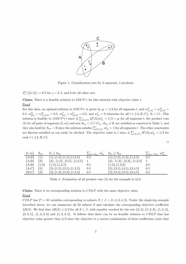
3.4 A tree structure for consideration sets

We seek to obtain a structural result on when CDLP and SDCP+ are equivalent. To that end, we define

a bipartite intersection graph of the consideration sets as follows: There are two types of nodes, one type

called segment node, the other is called intersection node. Each node of the former type corresponds to a

segment, each of the latter represents a set of the form Ck ∩ Cl for some segment pair (k, l). If a set S is

the intersection of two distinct pairs S = Cm ∩Cn = Ck ∩Cl, then S is represented by a single node. Edges

from segment k node connect to all the sets of the form Ck ∩ Cl 6= ∅.

The example of §3.3 has a cycle as can be seen from Figure 2. This turns out to be the critical feature:

If the segment consideration sets do not have a cycle, arranged say in the form of a tree (or, in general, a

forest), then the product cuts are sufficient to ensure equivalence between CDLP and SDCP+.

A

B

C

{1,2}=CA∩CB

{3}=CB∩CC

{5}=CA∩CC

Figure 2: Intersection graph for the example in §3.3.

3.5 Equivalence for tree overlapping consideration sets

We show in this section that if the intersection graph is a forest then SDCP+ = CDLP . To provide some

intuition behind this result, note that the intersection tree tells us which segments are directly or indirectly

connected to each other, in the sense that a solution wl for some segment l has implications on the solution

wk for all segment nodes k that are reachable from segment node l. The product cuts synchronize the

segment-level sub-solutions with respect to their weights, so that for a tree-structured intersection graph it

is possible for a given wl to arrange the segment-level solutions wk for all segments k reachable from l, in

a way such that they represent the projections of a feasible global solution onto the respective segments.

However, if there is a cycle then the offer set implications along that cycle can lead to a contradiction since

the product cuts do not synchronize segment-level solutions with respect to which sets can be offered in

parallel so as to guarantee the existence of a global offer set solution.

8

This was illustrated in Example 3.3, where the sets SA1 = {1, 2}, SB

1 = {1, 2, 3}, and SC1 = {3, 5} are

offered in parallel, but SC1 would require the product 5 to be offered on segment A as well, which creates

a contradiction and thus indicates that these segment-level solutions do not have a corresponding CDLP

solution.

AB

U

wA(S1)

wA(S2) w

B(S3)

wB(S4)

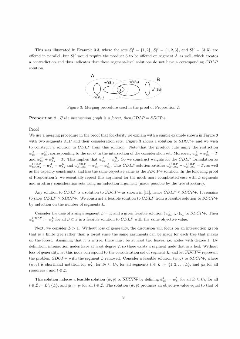
Figure 3: Merging procedure used in the proof of Proposition 2.

Proposition 2. If the intersection graph is a forest, then CDLP = SDCP+.

Proof

We use a merging procedure in the proof that for clarity we explain with a simple example shown in Figure 3

with two segments A,B and their consideration sets. Figure 3 shows a solution to SDCP+ and we wish

to construct a solution to CDLP from this solution. Note that the product cuts imply the restriction

wAS2

= wBS3, corresponding to the set U in the intersection of the consideration set. Moreover, wA

S1+wA

S2= T

and wBS3

+ wBS4

= T . This implies that wAS1

= wBS4. So we construct weights for the CDLP formulation as

wCDLPS1∪S4

= wAS1

= wBS4

and wCDLPS2∪S3

= wAS2

= wAS3. This CDLP solution satisfies wCDLP

S1∪S4+wCDLP

S2∪S3= T , as well

as the capacity constraints, and has the same objective value as the SDCP+ solution. In the following proof

of Proposition 2, we essentially repeat this argument for the much more complicated case with L segments

and arbitrary consideration sets using an induction argument (made possible by the tree structure).

Any solution to CDLP is a solution to SDCP+ as shown in [11], hence CDLP ≤ SDCP+. It remains

to show CDLP ≥ SDCP+. We construct a feasible solution to CDLP from a feasible solution to SDCP+

by induction on the number of segments L.

Consider the case of a single segment L = 1, and a given feasible solution (wLSL

, yL)SLto SDCP+. Then

wCDLPS := wL

S for all S ⊂ J is a feasible solution to CDLP with the same objective value.

Next, we consider L > 1. Without loss of generality, the discussion will focus on an intersection graph

that is a finite tree rather than a forest since the same arguments can be made for each tree that makes

up the forest. Assuming that it is a tree, there must be at least two leaves, i.e. nodes with degree 1. By

definition, intersection nodes have at least degree 2, so there exists a segment node that is a leaf. Without

loss of generality, let this node correspond to the consideration set of segment L, and let SDCP+ represent

the problem SDCP+ with the segment L removed. Consider a feasible solution (w, y) to SDCP+, where

(w, y) is shorthand notation for wlSl

for Sl ⊆ Cl, for all segments l ∈ L := {1, 2, . . . , L}, and yil for all

resources i and l ∈ L.

This solution induces a feasible solution (w, y) to SDCP+ by defining wlSl

:= wlSl

for all Sl ⊆ Cl, for all

l ∈ L := L \ {L}, and yl := yl for all l ∈ L. The solution (w, y) produces an objective value equal to that of

9

SDCP+ less∑

SL⊆CLλLR

L(SL)wLSL

. By the induction assumption, there exists a feasible solution wCDLPS

for all S ⊆ J := ∪L−1l=1 Cl to CDLP with the same objective value, and wCDLP induces (w, y) meaning that

wlSl

=∑

S⊆J|S∩Cl=SlwCDLP

S for all l ∈ L, Sl ⊆ Cl for l ∈ L, and yl =∑

Sl⊆Clλl

~Ql(Sl)wlSl

for all l ∈ L.

Now we construct a feasible solution wCDLPS for all S ⊂ J to CDLP that induces (w, y) for SDCP+

with same objective value. Since L is a leaf of the intersection tree, all interactions with other segments

are via a set Sint that is associated with the intersection node to which L is connected. Let us denote all

segments that are connected to this intersection node by Lint.

Consider a set U ⊆ Sint that is maximal for segment L with respect to Sint, that is there is no set SL ⊆ CL

such that U ( SL ∩ Sint and positive support wLSL

> 0. Note that for a feasible solution to SDCP+, the

product cuts ensure that if a set is maximal for L with respect to Sint, it is maximal for all segments l ∈ Lint

with respect to Sint. Moreover, from the definition of maximal

∑

{Sl⊆Cl|Sl∩Sint⊇U}

wlSl

=∑

{Sl⊆Cl|Sl∩Sint=U}

wlSl, ∀l ∈ Lint.

We select an arbitrary maximal set U ⊆ Sint and segment l ∈ Lint. The following argument shows that the

total weight τ(U) that we offer sets that intersect with Sint exactly in U is the same in solutions wL and

wCDLP :

τ(U) =∑

SL⊆CL|SL∩Sint=U

wLSL

(4)

=∑

Sl⊆Cl|Sl∩Sint=U

wlSl

(5)

=∑

Sl⊆Cl|Sl∩Sint=U

wlSl

(6)

=∑

Sl⊆Cl|Sl∩Sint=U

∑

S⊆J|S∩Cl=Sl

wCDLPS (7)

=∑

S⊆J|S∩Sint=U

wCDLPS .

The first equality holds by definition, the second due to maximality and the product cuts being satisfied by

the solution w to SDCP+, the third since wlSl

= wlSl, the fourth because wCDLP induces w, and the final

one as a result of a reformulation.

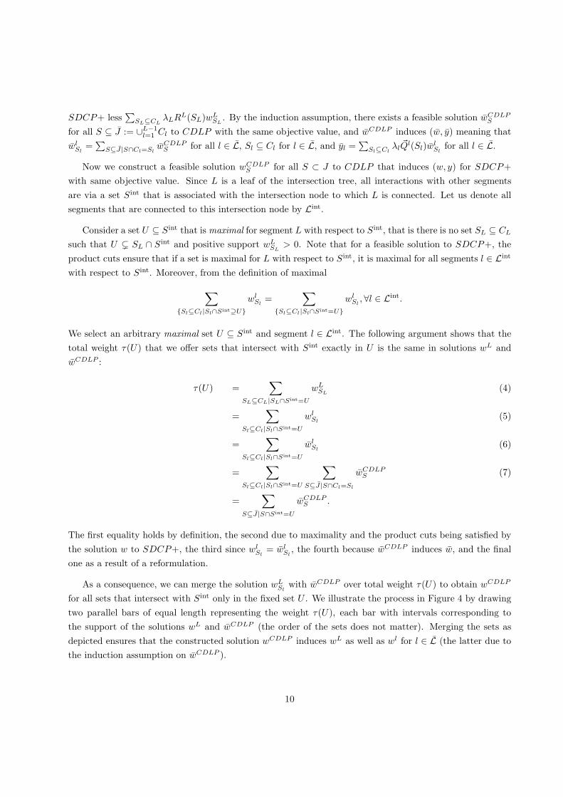
As a consequence, we can merge the solution wLSl

with wCDLP over total weight τ(U) to obtain wCDLP

for all sets that intersect with Sint only in the fixed set U . We illustrate the process in Figure 4 by drawing

two parallel bars of equal length representing the weight τ(U), each bar with intervals corresponding to

the support of the solutions wL and wCDLP (the order of the sets does not matter). Merging the sets as

depicted ensures that the constructed solution wCDLP induces wL as well as wl for l ∈ L (the latter due to

the induction assumption on wCDLP ).

10

wCDLPS1∪S4

wCDLPS2∪S4

wCDLPS2∪S5

wCDLPS3∪S5

wLS1

wLS2

wLS3

wCDLPS4

wCDLPS5

Figure 4: Illustration of the procedure to merge solutions in the support of wL and wCDLP to obtain wCDLP

for a fixed set U ⊆ Sint.

Now remove all the solution components wLSL

and wlSl

with positive support for all l ∈ Lint with Sl∩Sint =

U and SL ∩ Sint = U . After the removal, the product cut equations for the remaining solution remain valid

because of the equalities (4–5). We repeat this merging process by taking a maximal U ⊆ Sint at each stage

till we conclude with U = ∅. At every stage, as U is a maximal set, all the sets that contained U , namely

sets of the form U ( Sl ∩ Sint, l ∈ Lint were maximal sets in previous stages and therefore accounted for

by equalities (4–5) for the set Sl; now combining it with the product cuts for the set U , we again obtain

equalities (4–5).

The solution wCDLP that emerges from this process is feasible to CDLP : it holds that∑

U⊆Sint τ(U) = T

(note that U = ∅ ⊂ Sint), and therefore, by construction,∑

S wCDLPS = T . That the capacity constraint

of CDLP is satisfied follows from the induction assumption that wCDLP induces (w, y), with w := w and

y := y, combined with the fact that (w, y) is feasible to SDCP+ and that we constructed wCDLP in a

way such that we only added capacity consumption equal to that of segment L under solution wL. So the

combined solution also satisfies the induction for L segments.

The objective value of CDLP equals that of SDCP+ because in the merging process we only add prod-

ucts of CL \ Sint to the solution wCDLP , and since these products do not influence other segments as they

are only in the consideration set of segment L, we only add the contribution of segment L to the objective

without a change of the contribution of other segments.

✷

4 A numerical example in the literature

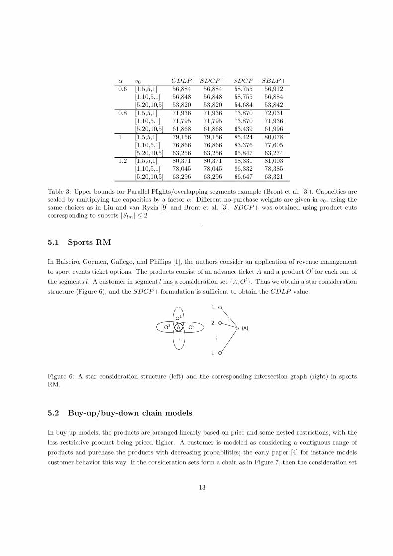
In this section we examine a test network used first in Liu and van Ryzin [9] and Bront et al. [3], and later

in Talluri [17], Meissner et al. [11] and Meissner and Strauss [10]. For brevity, we just give the bare details

of the network, specifically the consideration sets and the segments. We also give the value of a formulation

called SBLP+ that was derived by Talluri [17]. SBLP+ applies the product-cuts to a compact formulation

11

called sales-based linear program (SBLP ) due to Gallego et al. [6], and it is interesting to observe that this

formulation does not give CDLP value even with tree intersection structures, and we explain why at the

end of this section.

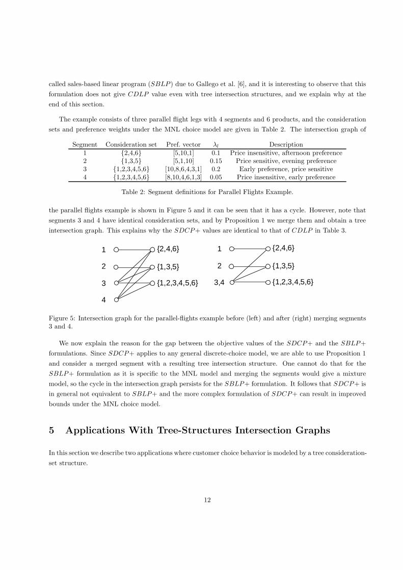
The example consists of three parallel flight legs with 4 segments and 6 products, and the consideration

sets and preference weights under the MNL choice model are given in Table 2. The intersection graph of

Segment Consideration set Pref. vector λl Description1 {2,4,6} [5,10,1] 0.1 Price insensitive, afternoon preference2 {1,3,5} [5,1,10] 0.15 Price sensitive, evening preference3 {1,2,3,4,5,6} [10,8,6,4,3,1] 0.2 Early preference, price sensitive4 {1,2,3,4,5,6} [8,10,4,6,1,3] 0.05 Price insensitive, early preference

Table 2: Segment definitions for Parallel Flights Example.

the parallel flights example is shown in Figure 5 and it can be seen that it has a cycle. However, note that

segments 3 and 4 have identical consideration sets, and by Proposition 1 we merge them and obtain a tree

intersection graph. This explains why the SDCP+ values are identical to that of CDLP in Table 3.

1

2

3

{2,4,6}

{1,3,5}

{1,2,3,4,5,6}

4

1

2

3,4

{2,4,6}

{1,3,5}

{1,2,3,4,5,6}

Figure 5: Intersection graph for the parallel-flights example before (left) and after (right) merging segments3 and 4.

We now explain the reason for the gap between the objective values of the SDCP+ and the SBLP+

formulations. Since SDCP+ applies to any general discrete-choice model, we are able to use Proposition 1

and consider a merged segment with a resulting tree intersection structure. One cannot do that for the

SBLP+ formulation as it is specific to the MNL model and merging the segments would give a mixture

model, so the cycle in the intersection graph persists for the SBLP+ formulation. It follows that SDCP+ is

in general not equivalent to SBLP+ and the more complex formulation of SDCP+ can result in improved

bounds under the MNL choice model.

5 Applications With Tree-Structures Intersection Graphs

In this section we describe two applications where customer choice behavior is modeled by a tree consideration-

set structure.

12

α v0 CDLP SDCP+ SDCP SBLP+0.6 [1,5,5,1] 56,884 56,884 58,755 56,912

[1,10,5,1] 56,848 56,848 58,755 56,884[5,20,10,5] 53,820 53,820 54,684 53,842

0.8 [1,5,5,1] 71,936 71,936 73,870 72,031[1,10,5,1] 71,795 71,795 73,870 71,936[5,20,10,5] 61,868 61,868 63,439 61,996

1 [1,5,5,1] 79,156 79,156 85,424 80,078[1,10,5,1] 76,866 76,866 83,376 77,605[5,20,10,5] 63,256 63,256 65,847 63,274

1.2 [1,5,5,1] 80,371 80,371 88,331 81,003[1,10,5,1] 78,045 78,045 86,332 78,385[5,20,10,5] 63,296 63,296 66,647 63,321

Table 3: Upper bounds for Parallel Flights/overlapping segments example (Bront et al. [3]). Capacities arescaled by multiplying the capacities by a factor α. Different no-purchase weights are given in v0, using thesame choices as in Liu and van Ryzin [9] and Bront et al. [3]. SDCP+ was obtained using product cutscorresponding to subsets |Slm| ≤ 2

.

5.1 Sports RM

In Balseiro, Gocmen, Gallego, and Phillips [1], the authors consider an application of revenue management

to sport events ticket options. The products consist of an advance ticket A and a product Ol for each one of

the segments l. A customer in segment l has a consideration set {A,Ol}. Thus we obtain a star consideration

structure (Figure 6), and the SDCP+ formulation is sufficient to obtain the CDLP value.

1

2

L

...

���

O1

O2 OLA

...

Figure 6: A star consideration structure (left) and the corresponding intersection graph (right) in sportsRM.

5.2 Buy-up/buy-down chain models

In buy-up models, the products are arranged linearly based on price and some nested restrictions, with the

less restrictive product being priced higher. A customer is modeled as considering a contiguous range of

products and purchase the products with decreasing probabilities; the early paper [4] for instance models

customer behavior this way. If the consideration sets form a chain as in Figure 7, then the consideration set

13

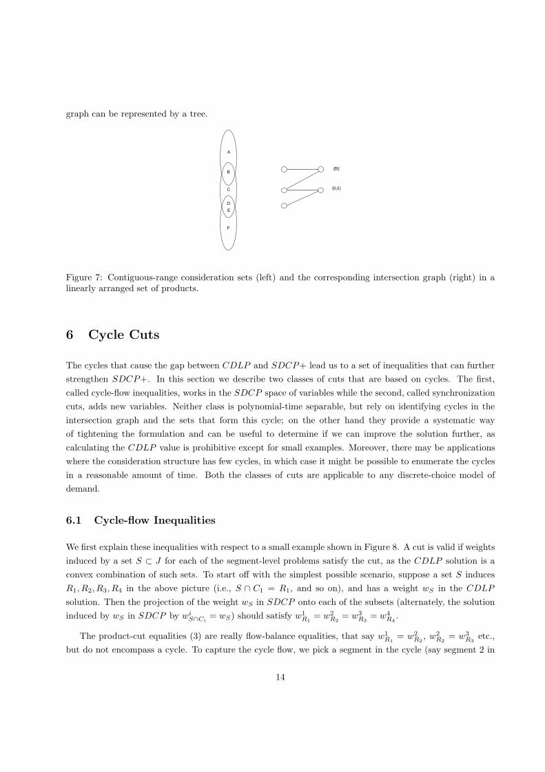
graph can be represented by a tree.

A

B

C

D

E

F

{B}

�����

Figure 7: Contiguous-range consideration sets (left) and the corresponding intersection graph (right) in alinearly arranged set of products.

6 Cycle Cuts

The cycles that cause the gap between CDLP and SDCP+ lead us to a set of inequalities that can further

strengthen SDCP+. In this section we describe two classes of cuts that are based on cycles. The first,

called cycle-flow inequalities, works in the SDCP space of variables while the second, called synchronization

cuts, adds new variables. Neither class is polynomial-time separable, but rely on identifying cycles in the

intersection graph and the sets that form this cycle; on the other hand they provide a systematic way

of tightening the formulation and can be useful to determine if we can improve the solution further, as

calculating the CDLP value is prohibitive except for small examples. Moreover, there may be applications

where the consideration structure has few cycles, in which case it might be possible to enumerate the cycles

in a reasonable amount of time. Both the classes of cuts are applicable to any discrete-choice model of

demand.

6.1 Cycle-flow Inequalities

We first explain these inequalities with respect to a small example shown in Figure 8. A cut is valid if weights

induced by a set S ⊂ J for each of the segment-level problems satisfy the cut, as the CDLP solution is a

convex combination of such sets. To start off with the simplest possible scenario, suppose a set S induces

R1, R2, R3, R4 in the above picture (i.e., S ∩ C1 = R1, and so on), and has a weight wS in the CDLP

solution. Then the projection of the weight wS in SDCP onto each of the subsets (alternately, the solution

induced by wS in SDCP by wiS∩Ci

= wS) should satisfy w1R1

= w2R2

= w3R3

= w4R4

.

The product-cut equalities (3) are really flow-balance equalities, that say w1R1

= w2R2

, w2R2

= w3R3

etc.,

but do not encompass a cycle. To capture the cycle flow, we pick a segment in the cycle (say segment 2 in

14

C1

C2

C3

C4

S23

S12

S34

S41

T2(S12, S23)

R2

R3

R4

R1

T2(S23, S12)

T3(S23, S34)

Figure 8: A cycle that induces S12 in C1 ∩ C2, S23 in C2 ∩ C3, S34 in C3 ∩ C4, S41 in C4 ∩ C1; setT 2(S12, 6⊂ S23) ⊆ C2 where T

2(S12, 6⊂ S23)∩C1 ⊇ S12 and T 2(S12, 6⊂ S23)∩C3 6⊇ S23; set T2(S23, 6⊂ S12) ⊆ C2

such that T 2(S23, 6⊂ S12)∩C3 ⊇ S23 and T 2(S23, 6⊂ S12)∩C1 6⊇ S12; setR2 ⊆ C2 such that R2∩(C1∩C2) ⊇ S12

and R2 ∩ (C2 ∩ C3) ⊇ S23, etc.

our running example) and derive some conditions that the flow in the cycle should satisfy.

There are two complications that come up in capturing the flow on the cycle. First, we have to sum

over all the sets of the form Ri that contain sets of the form Si,i+1 ⊂ Ci ∩ Ci+1. For this purpose, define

Ri(Si−1,i, Si,i+1) = {R ⊆ Ci|R ∩ Ci−1 ⊇ Si−1,i, R ∩ Ci+1 ⊇ Si,i+1} (if we index the segments in the cycle

1, . . . , k (so k is the length of the cycle), it should be understood that 0 corresponds to k and k+1 corresponds

to 1).

The second, and the more complicated part, comes up when S∩Ci leads to sets of the form T 2(S12, 6⊂ S23)

where T 2(S12, 6⊂ S23)∩C1 ⊇ S12 and T 2(S12, 6⊂ S23)∩C3 6⊇ S23 in Figure 8. A set S can presumably induce

R1, R3, R4 in segments 1, 3, 4 respectively and sets T 2(S12, 6⊂ S23) and T 2(S23, 6⊂ S12) in segment 2. So the

“flow” can go out of the cycle through sets such as these.

We account for this next. Define

T i(Si−1,i, 6⊂ Si,i+1) = {T ⊆ Ci|T ∩ Ci−1 ⊇ Si−1,i, T ∩ Ci+1 6⊇ Si,i+1}.

We define similarly T i(Si+1,i, 6⊂ Si−1,i).

For a given set of subsets in the intersections of the consideration sets of the cycle {Si,i+1 6= ∅}, we draw a

flow-graph with a node for each Si,i+1 and a set of arcs from Si−1,i to Si,i+1 representing the sum of weights

of the type Ri. In addition at each node there is a certain flow entering Si,i+1 made up of weights of sets

15

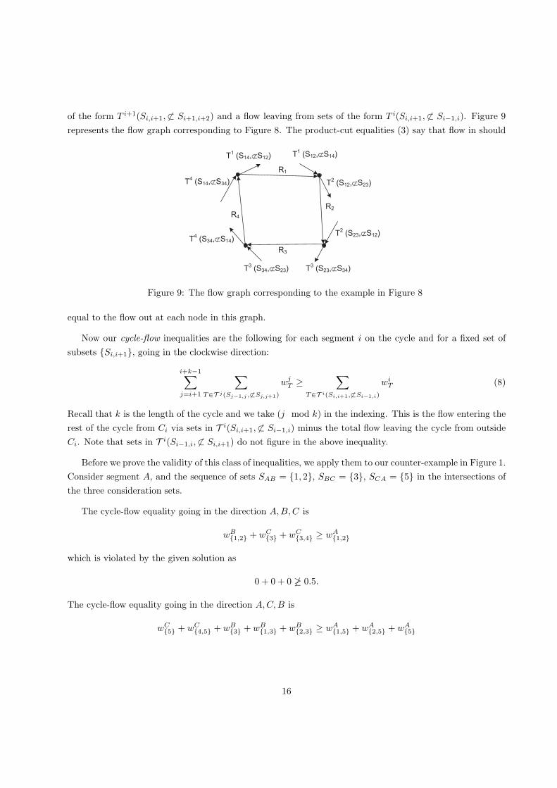
of the form T i+1(Si,i+1, 6⊂ Si+1,i+2) and a flow leaving from sets of the form T i(Si,i+1, 6⊂ Si−1,i). Figure 9

represents the flow graph corresponding to Figure 8. The product-cut equalities (3) say that flow in should

T2(S12, S23)

R2

R3

R4

R1

T2(S23, S12)

T3(S23, S34)T

3(S34, S23)

T4(S34, S14)

T4(S14, S34)

T1(S14, S12) T

1(S12, S14)

Figure 9: The flow graph corresponding to the example in Figure 8

equal to the flow out at each node in this graph.

Now our cycle-flow inequalities are the following for each segment i on the cycle and for a fixed set of

subsets {Si,i+1}, going in the clockwise direction:

i+k−1∑

j=i+1

∑

T∈T j(Sj−1,j , 6⊂Sj,j+1)

wjT ≥

∑

T∈T i(Si,i+1, 6⊂Si−1,i)

wiT (8)

Recall that k is the length of the cycle and we take (j mod k) in the indexing. This is the flow entering the

rest of the cycle from Ci via sets in T i(Si,i+1, 6⊂ Si−1,i) minus the total flow leaving the cycle from outside

Ci. Note that sets in T i(Si−1,i, 6⊂ Si,i+1) do not figure in the above inequality.

Before we prove the validity of this class of inequalities, we apply them to our counter-example in Figure 1.

Consider segment A, and the sequence of sets SAB = {1, 2}, SBC = {3}, SCA = {5} in the intersections of

the three consideration sets.

The cycle-flow equality going in the direction A,B,C is

wB{1,2} + wC

{3} + wC{3,4} ≥ wA

{1,2}

which is violated by the given solution as

0 + 0 + 0 6≥ 0.5.

The cycle-flow equality going in the direction A,C,B is

wC{5} + wC

{4,5} + wB{3} + wB

{1,3} + wB{2,3} ≥ wA

{1,5} + wA{2,5} + wA

{5}

16

which is also violated by the given solution as

0 + 0 + 0 + 0 + 0 6≥ 0 + 0.5 + 0.

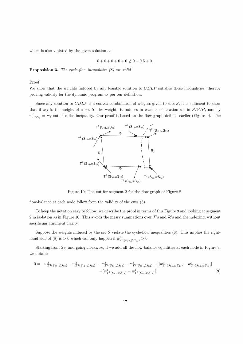
Proposition 3. The cycle-flow inequalities (8) are valid.

Proof

We show that the weights induced by any feasible solution to CDLP satisfies these inequalities, thereby

proving validity for the dynamic program as per our definition.

Since any solution to CDLP is a convex combination of weights given to sets S, it is sufficient to show

that if wS is the weight of a set S, the weights it induces in each consideration set in SDCP , namely

wiS∩Ci

= wS satisfies the inequality. Our proof is based on the flow graph defined earlier (Figure 9). The

T2(S12, S23)

R2

R3

R4

R1

T2(S23, S12)

T3(S23, S34)

T3(S34, S23)

T4(S34, S14)

T4(S14, S34)

T1(S14, S12) T

1(S12, S14)

Figure 10: The cut for segment 2 for the flow graph of Figure 8

flow-balance at each node follow from the validity of the cuts (3).

To keep the notation easy to follow, we describe the proof in terms of this Figure 9 and looking at segment

2 in isolation as in Figure 10. This avoids the messy summations over T ’s and R’s and the indexing, without

sacrificing argument clarity.

Suppose the weights induced by the set S violate the cycle-flow inequalities (8). This implies the right-

hand side of (8) is > 0 which can only happen if w2T 2(S23, 6⊂S12)

> 0.

Starting from S23 and going clockwise, if we add all the flow-balance equalities at each node in Figure 9,

we obtain:

0 = w2T 2(S23, 6⊂S12)

− w2T 2(S12, 6⊂S23)

+ [w3T 3(S34, 6⊂S23)

− w3T 3(S23, 6⊂S34)

] + [w4T 4(S14, 6⊂S34)

− w4T 4(S34, 6⊂S14)

]

+[w1T 1(S12, 6⊂S14)

− w1T 1(S14, 6⊂S12)

]. (9)

17

Going counter-clockwise just reverses the signs of all the terms. From (9),

w2T 2(S12, 6⊂S23)

= w2T 2(S23, 6⊂S12)

+ [w3T 3(S34, 6⊂S23)

− w3T 3(S23, 6⊂S34)

] + [w4T 4(S14, 6⊂S34)

− w4T 4(S34, 6⊂S14)

]

+[w1T 1(S12, 6⊂S14)

− w1T 1(S14, 6⊂S12)

]

≥ w2T 2(S23, 6⊂S12)

− w3T 3(S23, 6⊂S34)

− w4T 4(S34, 6⊂S14)

− w1T 1(S14, 6⊂S12)

> 0,

where the strict inequality is due to our assumption that the right-hand side of (8) is > 0. Our basic

observation is the following: For any set of weights of subsets in segment 2’s consideration set induced by a

set S, at most one of these w2T 2(S23, 6⊂S12)

, w2T 2(S12, 6⊂S23)

, w2R2

can have a positive value, simply because a set

S cannot intersect C2 in two different ways.

So we cannot have w2T 2(S12, 6⊂S23)

> 0 and we derive a contradiction.

✷

6.2 Cycle-synchronization Inequalities

In this section we propose another class of valid inequalities called the synchronization cuts that tighten the

SDCP+ bound when cycles are present in the intersection graph.

We illustrate the idea underlying the cuts on the example in §3.3 with the SDCP+ solution values:

wA{1,2} = wA

{2,5} = 0.5, wB{2} = wB

{1,2,3} = 0.5, wC{4} = wC

{3,5} = 0.5, and wlSl

= 0 otherwise for all l ∈

{A,B,C}, Sl ⊂ Cl. We pick an arbitrary segment on the cycle in the support of this solution, say segment

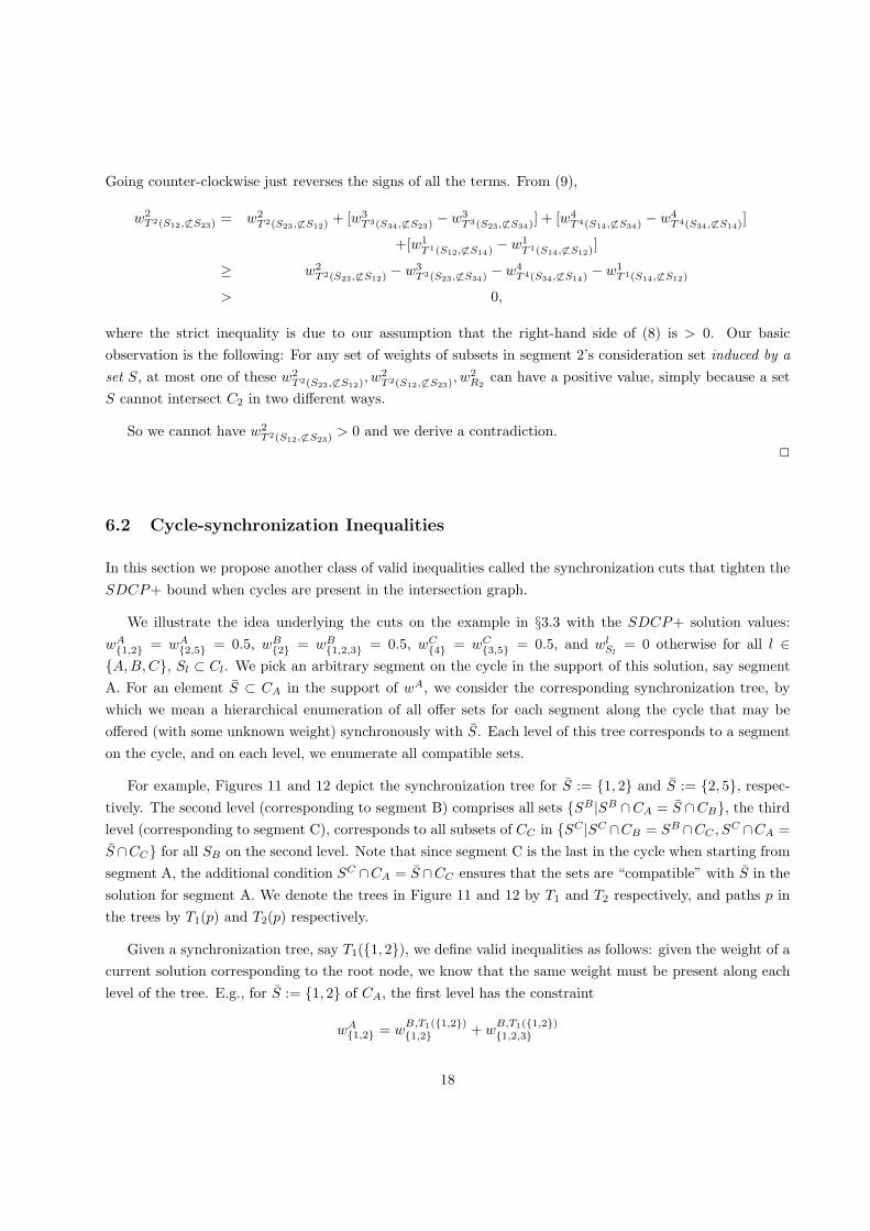
A. For an element S ⊂ CA in the support of wA, we consider the corresponding synchronization tree, by

which we mean a hierarchical enumeration of all offer sets for each segment along the cycle that may be

offered (with some unknown weight) synchronously with S. Each level of this tree corresponds to a segment

on the cycle, and on each level, we enumerate all compatible sets.

For example, Figures 11 and 12 depict the synchronization tree for S := {1, 2} and S := {2, 5}, respec-

tively. The second level (corresponding to segment B) comprises all sets {SB|SB ∩CA = S ∩CB}, the third

level (corresponding to segment C), corresponds to all subsets of CC in {SC |SC ∩CB = SB ∩CC , SC ∩CA =

S ∩CC} for all SB on the second level. Note that since segment C is the last in the cycle when starting from

segment A, the additional condition SC ∩CA = S ∩CC ensures that the sets are “compatible” with S in the

solution for segment A. We denote the trees in Figure 11 and 12 by T1 and T2 respectively, and paths p in

the trees by T1(p) and T2(p) respectively.

Given a synchronization tree, say T1({1, 2}), we define valid inequalities as follows: given the weight of a

current solution corresponding to the root node, we know that the same weight must be present along each

level of the tree. E.g., for S := {1, 2} of CA, the first level has the constraint

wA{1,2} = w

B,T1({1,2}){1,2} + w

B,T1({1,2}){1,2,3}

18

associated with it. Note that we need to introduce new tree-specific variables wB,T1({1,2}){1,2} and w

B,T1({1,2}){1,2,3}

since the sets {1,2} and {1,2,3} for segment B might only be synchronous with {1,2} on segment A for a

fraction of the overall offer weight. However, we do know that for the current given SDCP+ solution, it

must hold that these two new variables are bounded from above via wB,T1({1,2}){1,2} ≤ wB

{1,2} and wB,T1({1,2}){1,2,3} ≤

wB{1,2,3}. The same logic applies to the remaining branches, overall giving the following valid inequalities

associated with the synchronization tree in Figure 11:

wA{1,2} = w

B,T1({1,2}){1,2} + w

B,T1({1,2}){1,2,3} (10)

wB,T1({1,2}){1,2} ≤ wB

{1,2} (11)

wB,T1({1,2}){1,2,3} ≤ wB

{1,2,3} (12)

wB,T1({1,2}){1,2,3} = w

C,T1({1,2},{1,2,3}){3} + w

C,T1({1,2},{1,2,3}){3,4} (13)

wC,T1({1,2},{1,2,3}){3} ≤ wC

{3} (14)

wC,T1({1,2},{1,2,3}){3,4} ≤ wC

{3,4} (15)

wB,T1({1,2}){1,2} = w

C,T1({1,2},{1,2})∅ + w

C,T1({1,2},{1,2}){4}

wC,T1({1,2},{1,2})∅ ≤ wC

∅

wC,T1({1,2},{1,2}){4} ≤ wC

{4}.

(16)

For the current solution (wl) as defined above, equation (10) is satisfied wA{1,2} = 0.5 = 0 + 0.5 since (11)

requires wB,T1({1,2}){1,2} = 0 and (12) allows w

B,T1({1,2}){1,2,3} = 0.5. However, equation (13) is violated because

wB,T1({1,2}){1,2,3} = 0.5 6= 0 + 0; the right-hand side is zero because of inequalities (14–15).

Therefore, having found a violated constraint, we could add this constraint along with the constraints for

higher levels of the same tree to SDCP+ and re-solve. We are still guaranteed an upper bound on CDLP

because a feasible CDLP solution can always be projected onto the consideration sets of each segment

so that all synchronization cuts are satisfied for certain weights. In the current formulation, we require

Segment A

Segment B

Segment C

{1,2}

{1,2}

∅ {4}

{1,2,3}

{3} {3,4}

Figure 11: Full synchronization tree for SA = {1, 2}.

Segment A

Segment B

Segment C

{2,5}

{2}

{5} {4,5}

{2,3}

{3,5} {3,4,5}

Figure 12: Full synchronization tree for SA = {2, 5}.

an undesirably large number of additional variables (one per node in the synchronization tree). This can

19

be remedied to some extent in two steps: first, note that all products that are considered by exactly one

segment only can be removed from the tree, as they do not play a role as far as the offer set synchronization

is concerned.

For example, product 4 is the only product consider by exactly one segment, hence we can remove it from

the trees to obtain the reduced trees in Figures 13 and 14. The arising synchronization cuts corresponding

to S := {1, 2} are:

wA{1,2} = w

B,T1({1,2}){1,2} + w

B,T1({1,2}){1,2,3}

wB,T1({1,2}){1,2} ≤ wB

{1,2}

wB,T1({1,2}){1,2,3} ≤ wB

{1,2,3}

wB,T1({1,2}){1,2,3} = w

C,T1({1,2},{1,2,3}){3}

wC,T1({1,2},{1,2,3}){3} ≤ wC

{3} + wC{3,4}

wB,T1({1,2}){1,2} = w

C,T1({1,2},{1,2})∅

wC,T1({1,2},{1,2})∅ ≤ wC

∅ + wC{4}.

The SDCP+ solution still violates these constraints, so that adding them will tighten the bound. The

Segment A

Segment B

Segment C

{1,2}

{1,2}

∅

{1,2,3}

{3}

Figure 13: Reduced synchronization tree for SA ={1, 2}.

Segment A

Segment B

Segment C

{2,5}

{2}

{5}

{2,3}

{3,5}

Figure 14: Reduced synchronization tree for SA ={2, 5}.

number of additional variables can be reduced further; in fact, we can obtain valid inequalities by introducing

only one variable yT1p for each path p from the root SA to each leaf of the reduced synchronization tree (rather

than for each node). We illustrate this approach on the example in Figure 13: preservation of flow dictates

that

wA{1,2} =

∑

p

yT1

p . (17)

The flow along path p is limited by the minimum over the flows on all edges contained in this path, which

itself is bounded by the weights wlSl

on each node in the tree. For the synchronization tree in Figure 13,

we have two paths, namely p1 : {1, 2} → {1, 2} → ∅ and p2 : {1, 2} → {1, 2, 3} → {3}. This gives us the

20

following inequalities:

yT1

p1≤ wB

{1,2} (18)

yT1

p1≤ wC

∅ + wC{4} (19)

yT1

p2≤ wB

{1,2,3} (20)

yT1

p2≤ wC

{3} + wC{3,4}. (21)

The constraints (17–21) are violated by the solution of our running example since wB{1,2} = 0 and wC

{3} +

wC{3,4} = 0 imply yT1

p1= yT1

p2= 0, so that the equality constraint

wA{1,2} = 0.5 6= 0 = yT1

p1+ yT1

p2

is violated.

Proposition 4. The constraints (17–21) are valid inequalities.

Proof

As we noted earlier, as any solution to CDLP is a convex combination of weights given to sets S, it is

sufficient to show that if wS is the weight of a set S, the weights it induces in each consideration set in

SDCP , namely wiS∩Ci

= wS , satisfy the inequalities. Also, to avoid needless notation and clutter, we show

the validity for the specific synchronization tree of Figure 13. All the new variables are specific to the tree

and therefore are independent of variables introduced for the other cuts.

Let S ⊆ J be a set with wS > 0 in a solution to CDLP , and let wlS∩Cl

:= wS and wlSl

:= 0, for

all Sl ⊂ Cl, Sl 6= S ∩ Cl, for all segments l along the cycle. The synchronization constraints (17–21) are

associated with Figure 13. If S ∩ CA 6= {1, 2}, then we can set yT1p = 0 for all paths p in this tree, and

all constraints are satisfied. Otherwise, we have S ∩ CA = {1, 2}, and we show that the induced weights

form a unique path in the tree with root in S ∩ CA. It holds that (S ∩ CB) ∩ CA = (S ∩ CA) ∩ CB , hence

the set SB = S ∩ CB is on the tree in level B. Next, (S ∩ CB) ∩ CC = (S ∩ CC) ∩ CB , and since also

(S ∩ CC) ∩ CA = (S ∩ CA) ∩ CC—note that this is the end of the cycle—, the node S ∩ CC is under the

branch of S ∩ CB. Therefore, there is exactly one path p along the tree with positive weights of wCDLPS at

every level, and setting yT1

p := wS and yT1p := 0 otherwise satisfies the constraints.

✷

7 Numerical Results

In this section we implement the two classes of cuts to examine their power and running times. All methods

were tested in Matlab R2012a, running on an Intel i7-2600K CPU at 3.4 GHz.

21

7.1 Overview of the Tested Methods

We conduct a numerical study on various test networks where we compare the values resulting from the

following (time-aggregated) approaches:

• CDLP : Defined in §3.1. As proposed by Bront et al. [3], we use their pricing heuristic to identify

new columns; if it does not find any more columns, then we use their mixed integer programming

formulation until optimality is reached. The column generation process uses the following stopping

criterion: stop if reduced cost is less or equal to 10−8 ∗ (current restricted objective + reduced cost).

• SDCP : Segment-based deterministic concave program as defined in §3.2.

• SDCP+: Segment-based deterministic concave program with product constraints (3) for subsets

|Slk| ≤ 2.

• SDCP+F : We solve SDCP+ and add any flow constraints of the form (8) that are violated by

searching over all segments i and all combinations of subsets {{S1,2}, {S2,3}, . . . , }, checking both

directions around each cycle, and re-solve. Our reported results are based on full enumeration of all

subsets Si,i+1 for each cycle , and each segment on the cycle when searching for violated constraints. If

there are many products in the overlap Ci ∩Ci+1, then a heuristic approach would need to be chosen.

We pre-computed the sets Ti since they have few elements and only depend on the definition of the

consideration sets.

• SDCP+S: We solve SDCP+ and add any synchronization constraints that are violated by its solution

as discussed in §6.2, and re-solve. The cycle constraints are generated as follows: for each cycle, we

define an arbitrary segment on the cycle as the root segment. For a given segment-level solution,

we generate inequalities for a synchronization tree with root in an offer set with positive weight (of

course only if the corresponding constraints have not been included yet). We use the formulation that

introduces only one additional variable for each leaf in the sync tree. The iterations are stopped once

no more violated constraints are found. Note that the tree structures can be pre-computed since they

only depend on the segments’ consideration sets.

7.2 Test Networks

We test the effectiveness of the various approaches on a small network with 3 resources, as well as on a larger

network.

7.2.1 Parallel Flights Example With a Cycle

The first network example consists of three parallel flight legs as shown in Figure 15 with initial leg capacity

100. On each flight there is a low and a high fare class, L and H, respectively, with fares as specified in

22

Table 4. We define three customer segments as in Table 5; the preference values for the no-purchase option

is assumed to be negligible (we set it to 0.001). The sales horizon consists of 100 time periods.

A B

Leg 1 (early morning)

Leg 2 (noon)

Leg 3 (early afternoon)

Figure 15: Parallel flights example with cycle.

Product Leg Class Fare1 1 L 502 1 H 703 2 L 1004 2 H 1105 3 L 506 3 H 70

Table 4: Product definitions for parallel flights example with cycle.

Segment Consideration set Pref. vector λl Description1 {1,2,3,4} [7,6,6,5] 0.23 Morning preference2 {3,4,5,6} [8,5,8,6] 0.26 Noon preference3 {1,5} [3,5] 0.2 Cheap flights only

Table 5: Segment definitions for the parallel flights example with cycle.

In Table 6 we report upper bounds on the optimal expected revenue obtained from our various approaches.

Both SDCP+F and SDCP+S remove the gap to CDLP completely. Runtimes are not reported since the

example is too small (< 0.01 seconds for all scenarios).

7.2.2 Two Hubs Network Example

To test the performance of the two classes of cuts with regard to both runtime and upper bound, we consider

a larger hub and spoke network of a type similar to the ones used in [11], but with segments defined to have

many cycles in the intersection tree. There are two hubs H1 and H2 connected with two flights at 11am and

3pm in each direction, and each hub is connected to B spokes each. From each spoke leave two flights to the

adjacent hub at 9am and 1pm, and two flights return at 11am and 3pm. The spokes around hub H1 (H2)

are labeled from 1 to B (from B + 1 to 2B).

23

α v0 SDCP SDCP+ SDCP+F SDCP+C CDLP ∆SDCP+ ∆SDCP+F ∆SDCP+S

0.6[0.01 0.01 0.01] 6378 5728 5610 5610 5610 2.1 0.0 0.0[0.1 0.1 0.1] 6272 5647 5553 5553 5553 1.7 0.0 0.0[0.2 0.2 0.2] 6158 5562 5492 5492 5492 1.3 0.0 0.0

0.8[0.01 0.01 0.01] 6378 5728 5610 5610 5610 2.1 0.0 0.0[0.1 0.1 0.1] 6272 5647 5553 5553 5553 1.7 0.0 0.0[0.2 0.2 0.2] 6158 5562 5492 5492 5492 1.3 0.0 0.0

1[0.01 0.01 0.01] 6378 5728 5610 5610 5610 2.1 0.0 0.0[0.1 0.1 0.1] 6272 5647 5553 5553 5553 1.7 0.0 0.0[0.2 0.2 0.2] 6158 5562 5492 5492 5492 1.3 0.0 0.0

1.2[0.01 0.01 0.01] 6378 5728 5610 5610 5610 2.1 0.0 0.0[0.1 0.1 0.1] 6272 5647 5553 5553 5553 1.7 0.0 0.0[0.2 0.2 0.2] 6158 5562 5492 5492 5492 1.3 0.0 0.0

1.4[0.01 0.01 0.01] 6378 5728 5610 5610 5610 2.1 0.0 0.0[0.1 0.1 0.1] 6272 5647 5553 5553 5553 1.7 0.0 0.0[0.2 0.2 0.2] 6158 5562 5492 5492 5492 1.3 0.0 0.0

Table 6: Upper bounds for Parallel Flights Example. “∆X” denotes the percentage gap to CDLP, computedby (X-CDLP)/CDLP*100. α is a scaling parameter for the leg capacities, and v0 denotes the no-purchasepreference vector.

All direct flights between a spoke and a hub are short-haul flights and those between hubs are long-haul.

Depending on the number of spokes per hub, B, the network consists of 8B + 4 flight legs. In Figure 16

represents an example with B = 2.

3

H1

1

2

H2

4

Figure 16: Two Hubs Network example with two hubs and B = 2 spokes each.

There are 4B2 + 6B + 2 origin-destination pairs (4B between spoke and hub around one hub, 2 between

hubs, 2B2 spoke to spoke via 2 hubs, 2B(B − 1) spoke to spoke via one hub, 2B hub to hub to spoke, and

2B spoke to hub via another hub).

There are 8B2 + 10B + 4 possible itineraries (8B between spoke and hub around one hub, 4 between

hubs, 2B2 between spoke and spoke via 2 hubs, 6B(B − 1) between spoke and spoke via 1 hub, 2B hub to

24

hub to spoke, 6B spoke to hub to hub). For example, the only itinerary between spoke 1 and spoke (B+1) is

the 9am flight 1→ H1, the 11am flight H1→ H2, and the 3pm flight H2→ (B +1). Other origin-destination

pairs can have up to three possible itineraries, for example going from spoke 1 to H2, or to B.

For each itinerary there are five booking classes Y, M, Q, G and T; hence we have 40B2 + 50B + 20

products in total. The fares are sampled from a Poisson distribution with mean depending on the type of

itinerary as reported in Table 7. If the fares are not in the order Y > M > Q > G > T , then we re-sample

until that order is obtained.

Itinerary Type Y M Q G Tshort-haul with 1 leg 100 90 60 40 30short-haul with 2 legs 200 180 120 80 60long-haul with 1 leg 300 270 180 120 90long-haul with 2 legs 400 360 240 160 120long-haul with 3 legs 500 450 300 200 150

Table 7: Mean fares for different itinerary types and booking classes.

The customer segments are defined as follows: for each origin-destination (OD) pair, there are between

one and three itineraries possible, and there is a customer segment for each itinerary considering all booking

classes on that itinerary only. These segments represent customers who are less price sensitive and not

flexible in their choice of itinerary. In addition, there is a segment of less price sensitive customers who are

flexible with regard to itinerary but not with regard to advance purchase requirements, so that this segment

considers classes Y and M for all itineraries for this OD. Likewise, a final segment for this OD consists of

customers who are price sensitive and flexible both in itinerary as well as in time, and hence only consider

the advance purchase classes G and T across all itineraries. Therefore, for every OD pair, we have between

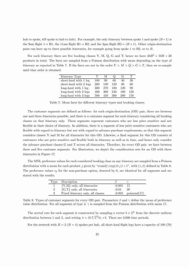
three and five customer segments. For illustration, we depict the consideration sets for an OD with three

itineraries in Figure 17.

The MNL preference values for each considered booking class on any itinerary are sampled from a Poisson

distribution with a mean for each product j given by “round(γ exp(βrj))+1”, with (γ,β) defined in Table 8.

The preference values v0 for the non-purchase option, denoted by 0, are identical for all segments and are

stated with the results.

Type Description β γ1 {Y,M} only, all itineraries -0.001 152 {G,T} only, all itineraries -0.01 203 Fixed itinerary only, all classes -0.005 poissrnd(17)

Table 8: Types of customer segments for every OD pair. Parameters β and γ define the mean of preferencevalue distribution. For all segments of type 3, γ is sampled from the Poisson distribution with mean 17.

The arrival rate for each segment is constructed by sampling a vector b ∈ ZL from the discrete uniform

distribution between 1 and L, and setting λ = (0.7/~1T b). ∗ b. There are 3,000 time periods.

For the network with B = 2 (B = 4) spokes per hub, all short-haul flight legs have a capacity of 100 (70)

25

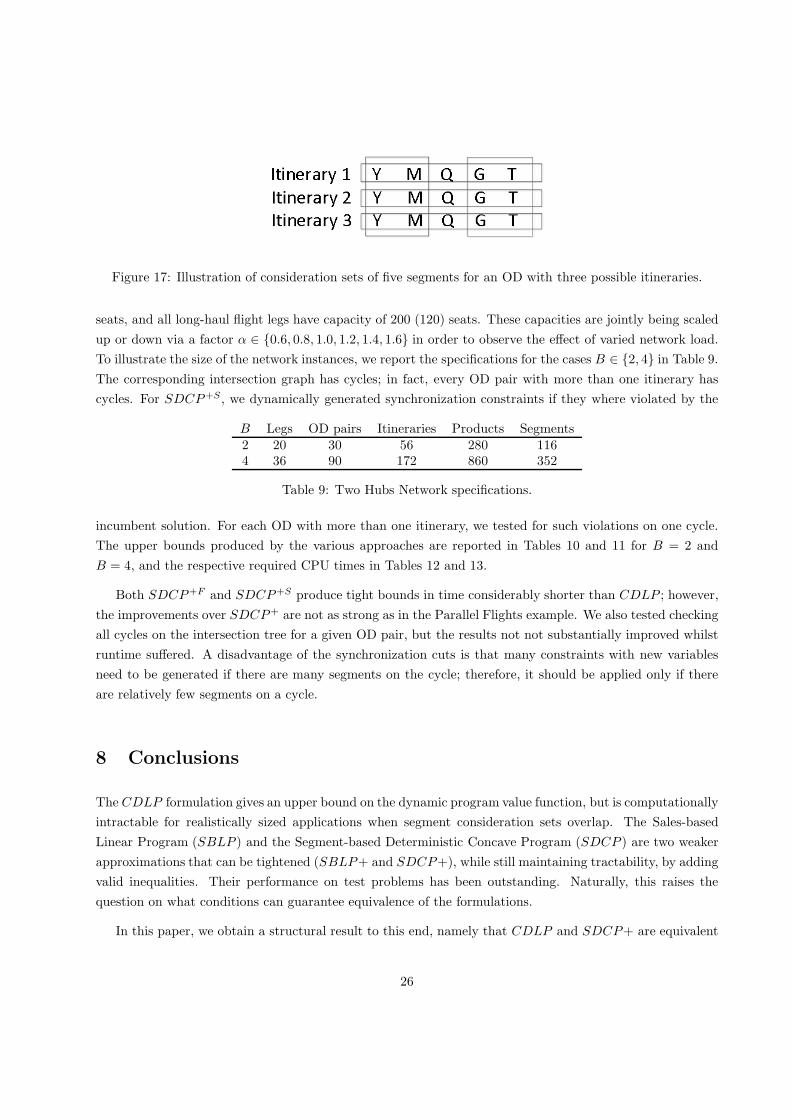
Figure 17: Illustration of consideration sets of five segments for an OD with three possible itineraries.

seats, and all long-haul flight legs have capacity of 200 (120) seats. These capacities are jointly being scaled

up or down via a factor α ∈ {0.6, 0.8, 1.0, 1.2, 1.4, 1.6} in order to observe the effect of varied network load.

To illustrate the size of the network instances, we report the specifications for the cases B ∈ {2, 4} in Table 9.

The corresponding intersection graph has cycles; in fact, every OD pair with more than one itinerary has

cycles. For SDCP+S, we dynamically generated synchronization constraints if they where violated by the

B Legs OD pairs Itineraries Products Segments2 20 30 56 280 1164 36 90 172 860 352

Table 9: Two Hubs Network specifications.

incumbent solution. For each OD with more than one itinerary, we tested for such violations on one cycle.

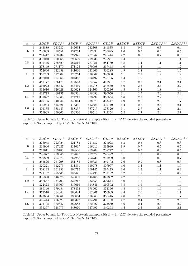
The upper bounds produced by the various approaches are reported in Tables 10 and 11 for B = 2 and

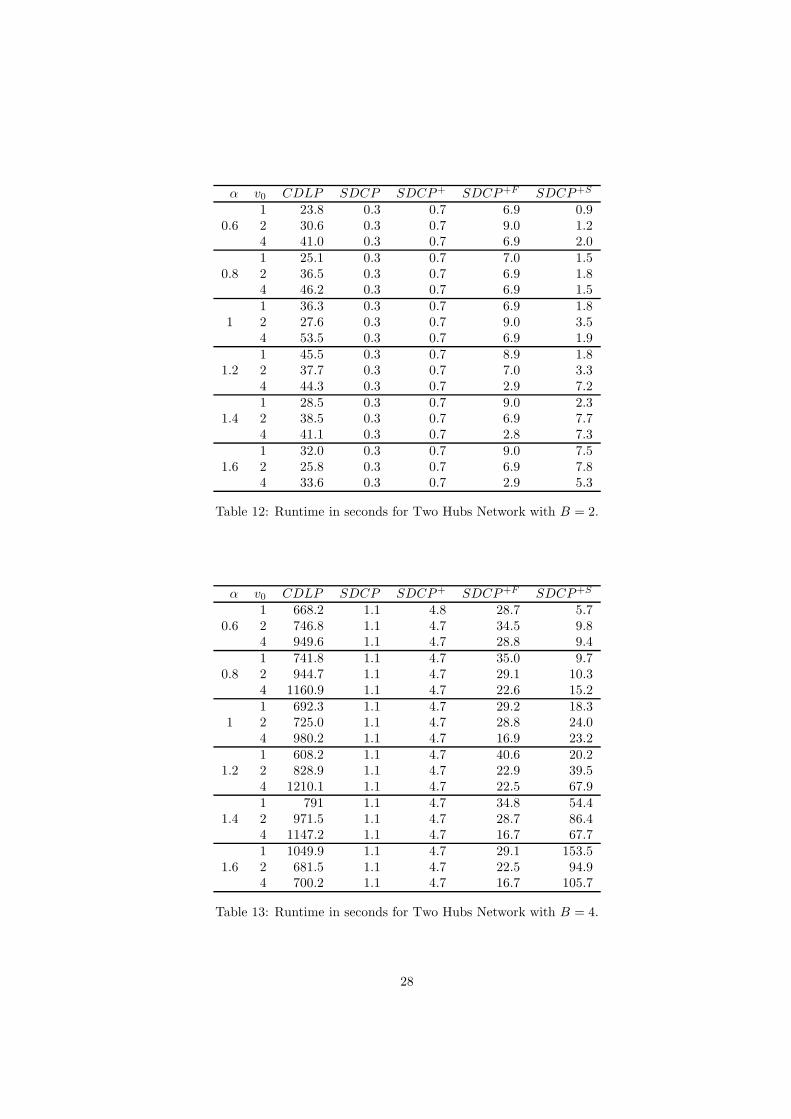
B = 4, and the respective required CPU times in Tables 12 and 13.

Both SDCP+F and SDCP+S produce tight bounds in time considerably shorter than CDLP ; however,

the improvements over SDCP+ are not as strong as in the Parallel Flights example. We also tested checking

all cycles on the intersection tree for a given OD pair, but the results not not substantially improved whilst

runtime suffered. A disadvantage of the synchronization cuts is that many constraints with new variables

need to be generated if there are many segments on the cycle; therefore, it should be applied only if there

are relatively few segments on a cycle.

8 Conclusions

The CDLP formulation gives an upper bound on the dynamic program value function, but is computationally

intractable for realistically sized applications when segment consideration sets overlap. The Sales-based

Linear Program (SBLP ) and the Segment-based Deterministic Concave Program (SDCP ) are two weaker

approximations that can be tightened (SBLP+ and SDCP+), while still maintaining tractability, by adding

valid inequalities. Their performance on test problems has been outstanding. Naturally, this raises the

question on what conditions can guarantee equivalence of the formulations.

In this paper, we obtain a structural result to this end, namely that CDLP and SDCP+ are equivalent

26

α v0 SDCP SDCP+ SDCP+F SDCP+S CDLP ∆SDCP ∆SDCP+ ∆SDCP+F ∆SDCP+S

0.61 244889 243232 242634 242708 241835 1.3 0.6 0.3 0.42 240609 238551 237764 237894 236825 1.6 0.7 0.4 0.54 231417 228234 227976 227847 226444 2.2 0.8 0.7 0.6

0.81 306040 300366 298699 299233 295861 3.4 1.5 1.0 1.12 295446 288829 287816 287981 284739 3.8 1.4 1.1 1.14 278149 271170 271123 270598 267448 4.0 1.4 1.4 1.2

11 352696 342458 341036 341369 336285 4.9 1.8 1.4 1.52 336233 327009 326254 326067 320030 5.1 2.2 1.9 1.94 312040 304363 304362 303497 298795 4.4 1.9 1.9 1.6

1.21 387777 376175 374663 374557 366891 5.7 2.5 2.1 2.12 366922 356647 356469 355278 347560 5.6 2.6 2.6 2.24 334616 326028 326028 324769 320236 4.5 1.8 1.8 1.4

1.41 413773 400737 400361 398483 390050 6.1 2.7 2.6 2.22 387027 374863 374719 373294 366554 5.6 2.3 2.2 1.84 349735 340044 340044 338970 333447 4.9 2.0 2.0 1.7

1.61 430934 415821 415341 413586 405149 6.4 2.6 2.5 2.12 401335 388445 388337 387215 378320 6.1 2.7 2.6 2.44 359965 350366 350366 349512 342254 5.2 2.4 2.4 2.1

Table 10: Upper bounds for Two Hubs Network example with B = 2. “∆X” denotes the rounded percentagegap to CDLP , computed by (X-CDLP )/CDLP*100.

α v0 SDCP SDCP+ SDCP+F SDCP+S CDLP ∆SDCP ∆SDCP+ ∆SDCP+F ∆SDCP+S

0.61 223958 222024 221782 221787 221028 1.3 0.5 0.3 0.32 219996 217427 217067 216912 215929 1.9 0.7 0.5 0.54 212611 209783 209506 209204 208247 2.1 0.7 0.6 0.5

0.81 278877 273846 272847 272572 270422 3.1 1.3 0.9 0.82 269869 264675 264288 263736 261989 3.0 1.0 0.9 0.74 255626 251298 251183 250636 249102 2.6 0.9 0.8 0.6

11 320221 312273 311331 310978 307957 4.0 1.4 1.1 1.02 308133 301253 300775 300145 297475 3.6 1.3 1.1 0.94 291107 285563 285471 284793 282182 3.2 1.2 1.2 0.9

1.21 355860 346876 345889 345483 341382 4.2 1.6 1.3 1.22 342687 334703 334212 333554 329644 4.0 1.5 1.4 1.24 322473 315660 315616 314841 310592 3.8 1.6 1.6 1.4

1.41 389140 379454 378452 378062 372356 4.5 1.9 1.6 1.52 372510 364044 363644 362967 356909 4.4 2.0 1.9 1.74 343654 336861 336834 336060 330415 4.0 2.0 1.9 1.7

1.61 415444 406025 405327 404791 396708 4.7 2.4 2.2 2.02 391198 382847 382683 382022 373839 4.6 2.4 2.4 2.24 355267 348075 348070 347497 340263 4.4 2.3 2.3 2.1

Table 11: Upper bounds for Two Hubs Network example with B = 4. “∆X” denotes the rounded percentagegap to CDLP , computed by (X-CDLP )/CDLP*100.

27

α v0 CDLP SDCP SDCP+ SDCP+F SDCP+S

0.61 23.8 0.3 0.7 6.9 0.92 30.6 0.3 0.7 9.0 1.24 41.0 0.3 0.7 6.9 2.0

0.81 25.1 0.3 0.7 7.0 1.52 36.5 0.3 0.7 6.9 1.84 46.2 0.3 0.7 6.9 1.5

11 36.3 0.3 0.7 6.9 1.82 27.6 0.3 0.7 9.0 3.54 53.5 0.3 0.7 6.9 1.9

1.21 45.5 0.3 0.7 8.9 1.82 37.7 0.3 0.7 7.0 3.34 44.3 0.3 0.7 2.9 7.2

1.41 28.5 0.3 0.7 9.0 2.32 38.5 0.3 0.7 6.9 7.74 41.1 0.3 0.7 2.8 7.3

1.61 32.0 0.3 0.7 9.0 7.52 25.8 0.3 0.7 6.9 7.84 33.6 0.3 0.7 2.9 5.3

Table 12: Runtime in seconds for Two Hubs Network with B = 2.

α v0 CDLP SDCP SDCP+ SDCP+F SDCP+S

0.61 668.2 1.1 4.8 28.7 5.72 746.8 1.1 4.7 34.5 9.84 949.6 1.1 4.7 28.8 9.4

0.81 741.8 1.1 4.7 35.0 9.72 944.7 1.1 4.7 29.1 10.34 1160.9 1.1 4.7 22.6 15.2

11 692.3 1.1 4.7 29.2 18.32 725.0 1.1 4.7 28.8 24.04 980.2 1.1 4.7 16.9 23.2

1.21 608.2 1.1 4.7 40.6 20.22 828.9 1.1 4.7 22.9 39.54 1210.1 1.1 4.7 22.5 67.9

1.41 791 1.1 4.7 34.8 54.42 971.5 1.1 4.7 28.7 86.44 1147.2 1.1 4.7 16.7 67.7

1.61 1049.9 1.1 4.7 29.1 153.52 681.5 1.1 4.7 22.5 94.94 700.2 1.1 4.7 16.7 105.7

Table 13: Runtime in seconds for Two Hubs Network with B = 4.

28

if the intersection graph of the segment consideration sets is a tree (or a forest). This implies that these

efficient solution methods will be guaranteed to yield the same control policies as CDLP if demand can be

modeled without cycles in the overlap structure of the segment consideration sets.

For consideration set structures with cycles, we propose two classes of valid inequalities that are rela-

tively easy to generate systematically and which tighten the upper bounds on the optimal expected revenue

significantly. We conduct extensive numerical experiments to validate the performance of these classes of

cuts. Our structural result and the valid inequalities are applicable for all discrete choice models.

References

[1] Balseiro, S., C. Gocmen, G. Gallego, R. Phillips. 2011. Revenue management of consumer options for

sporting events. Tech. rep., IEOR, Columbia University, New York.

[2] Bodea, T., M. Ferguson, L. Garrow. 2009. Choice-based revenue management: Data from a major hotel

chain. Manufacturing & Service Operations Management 11 356–361.

[3] Bront, J. J. M., I. Mendez-Dıaz, G. Vulcano. 2009. A column generation algorithm for choice-based

network revenue management. Operations Research 57(3) 769–784.

[4] Brumelle, S. L., J. I. McGill, T. H. Oum, K. Sawaki, M. W. Tretheway. 1990. Allocation of airline seat

between stochastically dependent demands. Transportation Science 24 183–192.

[5] Gallego, G., G. Iyengar, R. Phillips, A. Dubey. 2004. Managing flexible products on a network. Tech.

Rep. TR-2004-01, Dept of Industrial Engineering, Columbia University, NY, NY.

[6] Gallego, G., R. Ratcliff, S. Shebalov. 2010. A general attraction model and an efficient formulation for

network revenue management. Tech. rep., Department of IEOR, Columbia University.

[7] Kunnumkal, S. 2011. Randomization approaches for the network revenue management with customer

choice behavior. Tech. rep., Indian School of Business, Hyperabad, India.

[8] Kunnumkal, S., H. Topaloglu. 2010. A new dynamic programming decomposition method for the net-

work revenue management problem with customer choice behavior. Production and Operations Man-

agement 19 575–590.

[9] Liu, Q., G. van Ryzin. 2008. On the choice-based linear programming model for network revenue

management. Manufacturing and Service Operations Management 10(2) 288–310.

[10] Meissner, J., A. K. Strauss. 2012. Network revenue management with inventory-sensitive bid prices and

customer choice. European Journal of Operational Research 216 459–468.

[11] Meissner, J., A. K. Strauss, K. Talluri. 2011. An enhanced concave programming method for choice

network revenue management. Production and Operations Management (Forthcoming).

29

[12] Mendez-Dıaz, I., J. Miranda Bront, G. Vulcano, P. Zabala. 2012. A branch-and-cut algorithm for the

latent-class logit assortment problem. Forthcoming in Discrete Applied Mathematics.

[13] Rusmevichientong, P., D. Shmoys, H. Topaloglu. 2010. Assortment optimization with mixtures of logits.

Tech. rep., School of IEOR, Cornell University.

[14] Shocker, A.D., M. Ben-Akiva, B. Boccara, P. Nedungadi. 1991. Consideration set influences on consumer

decision-making and choice: Issues, models, and suggestions. Marketing Letters 2(3) 181–197.

[15] Talluri, K. T., G. J. van Ryzin. 2004. Revenue management under a general discrete choice model of

consumer behavior. Management Science 50(1) 15–33.

[16] Talluri, K. T., G. J. van Ryzin. 2004. The Theory and Practice of Revenue Management . Kluwer, New

York, NY.

[17] Talluri, K.T. 2010. A randomized concave programming method for choice network revenue manage-

ment. Tech. rep., Working Paper 1215, Department of Economics, Universitat Pompeu Fabra, Barcelona,

Spain.

[18] Zhang, D., D. Adelman. 2009. An approximate dynamic programming approach to network revenue

management with customer choice. Transportation Science 43(3) 381–394.

30